Uncovering the invariant structural organization of the human connectome

Abstract

In order to understand the complex cognitive functions of the human brain, it is essential to study the structural macro-connectome, i.e., the wiring of different brain regions to each other through axonal pathways, that has been revealed by imaging techniques. However, the high degree of plasticity and cross-population variability in human brains makes it difficult to relate structure to function, motivating a search for invariant patterns in the connectivity. At the same time, variability within a population can provide information about the generative mechanisms. In this paper we analyze the connection topology and link-weight distribution of human structural connectomes obtained from a database comprising $196$ subjects. By demonstrating a correspondence between the occurrence frequency of individual links and their average weight across the population, we show that the process by which the human brain is wired is not independent of the process by which the link weights of the connectome are determined. Furthermore, using the specific distribution of the weights associated with each link over the entire population, we show that a single parameter that is specific to a link can account for its frequency of occurrence, as well as, the variation in its weight across different subjects. This parameter provides a basis for “rescaling” the link weights in each connectome, allowing us to obtain a generic network representative of the human brain, distinct from a simple average over the connectomes. We obtain the functional connectomes by implementing a neural mass model on each of the vertices of the corresponding structural connectomes. By comparing these with the empirical functional brain networks, we demonstrate that the rescaling procedure yields a closer structure-function correspondence. Finally, we show that the representative network can be decomposed into a basal component that is stable across the population and a highly variable superstructure.

I Introduction

One of the key goals of neuroscience from its very inception has been to unravel the workings of the human brain. Not only is this of great scientific interest and significant from a philosophical perspective, but it is important also for informing clinical and psychiatric practice. Studying the nervous systems of non-human model organisms do allow us to gain an understanding of fundamental aspects of their development, structure and function. Moreover, this has provided us with numerous insights on how a system as complex as the brain could have evolved, and the associated emergence of behavior such as cognition. However, there are limitations to how phenomena observed in relatively simpler nervous systems can be generalized to those with much higher complexity. For instance the ocular dominance columns of the visual cortex that occur in monkey and cat brains are not seen in mice or rat brains. Horton2005 . Similarly, the anatomical and functional organization of a macaque brain is vastly different from that of a human brain Passingham2009 . In fact there are several fundamental aspects of human brain structure and function that are unique to the species Rilling2014 ; Kaas2013 . Therefore, in spite of the ethical and technological bottlenecks that hinder the study of the human brain to the level of detail and precision as can be achieved in other mammals and invertebrates, it is crucial that techniques for analyzing and interpreting the structure and function of human brains at multiple length and time scales continue to be developed and refined.

One of the primary approaches that is commonly used to study a brain is to describe its macro-scale connectome Sporns2005 , i.e., the structure of connectivity between distinct brain regions through axonal tracts. Several studies have pointed to the essential role of such a “wiring diagram” of the nervous system as a foundational model in understanding functional localization at multiple levels, ranging from molecular and cellular up to systems and behavioral levels Swanson2010 . As shown in Pathak2020a , the wiring diagrams of neuronal connectivity can provide insights on the processes that underlie brain development, as well as, the functional implications arising from their structural organization Pathak2020 . However, one of the characteristic features of the human structural connectome is its large variability across individuals Sporns2005 ; Llera2019 ; Smith2019 and over time Madole2020 . This variability in the structural connectome could be a key factor in understanding the generative mechanism underlying the development of brain structure Klimm2014 . The diversity in structural connectivity is significantly smaller than that of functional connectivity Kelly2012 ; Yan2013 , which is determined by temporal correlations between the electrophysiological activity of different brain regions. These variabilities are important in studying the relationship between structure and function in human brains, as not only is structural connectivity known to affect brain function Honey2009 ; Hagmann2008 , but function has been shown to influence the structure as well Mishra2019 ; Taya2015 . However, despite the high variability of brain networks in humans, it has been observed that certain structural features are universal Bullmore2009 . Thus, it is pertinent to ask whether we can describe a typical “representative” structural connectome for a human brain. Such a representative network might not only be useful in studying fundamental aspects of the structure-function relationship in the human brain, but also the deviations from this “basic plan” in a connectome might reveal structural correlates of functional impairments leading to clinical disorders.

In this work, we study a large ensemble of brain connectivity networks that were obtained from a cohort of $196$ healthy human subjects through diffusion tensor imaging for the purpose of characterizing the variability in the structural connectome. We find that there is a correspondence between the diversity of topological connectivities and the variation in the distribution of connection weights, suggesting that the generative mechanisms giving rise to the “wiring” and those determining the weights are related. We further find that the connection strengths of links that are frequently found in the population are described by link-specific Poisson processes, indicating that the generative mechanism of a significant portion of the brain connectivity might involve independent discrete random processes. This allows us to reassign the link weights of structural connectivity, which would represent the discrete Poisson variables instead of original weights and thus obtain the rescaled weight matrices. Using the corresponding resting state functional connectivities obtained from the same cohort, we show that the structural connectome with rescaled weights consistently show better correspondence with the functional connectivity, suggesting that the rescaling process might provide a more informative framework for interpreting the structural connectivity in terms of function. This also provides us with a means for determining the generic “representative” network describing a human connectome. Finally, we show that the representative network is intrinsically resolved into two components, one which is invariant across the population and another that exhibits a much higher degree of variability across individuals.

II Materials and Methods

II.1 Connectivity Data

The human brain structural and functional connectivity dataset analyzed here has been derived from the Nathan Kline Institute (NKI) / Rockland Sample Nooner2012 - a publicly available repository of diffusion tensor imaging (DTI) and resting state functional magnetic resonance imaging (rs-fMRI) data - which was further processed into connectivity matrices and made publicly available in the UCLA multimodal connectivity database at http://umcd.humanconnectomeproject.org/ Brown2012 .

The data comprises structural connectivity matrices $W$ and functional connectivity matrices $C$ obtained from $196$ healthy human subjects: $114$ male and $82$ female, with ages ranging from $4$ to $85$ years. Each matrix describes a network comprising $188$ nodes that represent 188 brain regions defined by parcellation of the entire gray matter region of the human brain (cerebral cortex, sub-cortical areas, cerebellum, brain stem etc.) using an fMRI based clustering method Craddock2012 . It also contains the $3$-dimensional coordinates for each of the brain regions in a standardized space. For structural connectivity (SC) matrices $W$, the connection strengths $W_{ij}$ corresponding to the weighted undirected links $(i,j)$ represent the density of axonal bundles between brain regions $i$ and $j$ as obtained from DTI, while the connection strengths $C_{ij}$ in functional connectivity matrices $C$ represent the Pearson’s correlation coefficients between the time-series of dynamical activities in regions $i$ and $j$, as measured through blood oxygen level dependent (BOLD) imaging using fMRI.

II.2 Rescaling to obtain Poisson distributed link weights

A Poisson distribution of mean $\lambda$ for a random discrete variable $X$ is given by:

$$P(X=k)=\frac{\lambda^{k}e^{-\lambda}}{k!}\,,$$ (1)

where the parameter characterizing the distribution $\lambda=\langle X\rangle=Var(X)$. Here the link weights $W_{ij}$ for a link between a pair of regions $(i,j)$ are considered to be obtained by rescaling Poisson distributed variables $\mathcal{W}_{ij}$ that have mean $\lambda_{ij}$, as $W_{ij}=s_{ij}\mathcal{W}_{ij}$. Such a rescaled Poisson variable has also been described in Prem2017 . The mean and variance of the rescaled Poisson variables $W_{ij}$ are given by:

$$\begin{split}\langle W_{ij}\rangle&=s_{ij}\lambda_{ij}\,,\\ Var(W_{ij})&=s^{2}_{ij}\lambda_{ij}\,,\end{split}$$ (2)

For a given distribution of weights $W_{ij}$ of a link $(i,j)$, we determine $s_{ij}$ from Eq. (2)

$$s_{ij}=\frac{Var(W_{ij})}{\langle W_{ij}\rangle}$$ (3)

Upon obtaining the rescaling factor $s_{ij}$ for a link $(i,j)$, we rescale the weights $W_{ij}$ across the population to obtain the Poisson distributed rescaled weights:

$$\mathcal{W}_{ij}=\lfloor\frac{W_{ij}}{s_{ij}}+0.5\rfloor$$ (4)

where $\lfloor x+0.5\rfloor$ gives nearest integer of $x$. The rescaled weights are related to the Poisson parameter by $\langle\mathcal{W}_{ij}\rangle=\lambda_{ij}$.

II.3 Goodness of fit

Assuming a rescaled Poisson distribution for all links $(i,j)$, we initially calculate the Poisson parameter $\lambda_{ij}$, rescaling factor $s_{ij}$ and the rescaled weights $\mathcal{W}_{ij}$ for each link. We then use a Pearson’s Chi-squared test Pearson1900 to determine whether the rescaled weights obtained using the method described above fits a theoretically expected Poisson distribution $\mathcal{P}(\lambda_{ij})$ for the corresponding $\lambda_{ij}$ with significant likelihood. First, we calculate the test statistic $\chi^{2}_{ij}$ for the rescaled weight frequency distribution of each link:

$$\chi^{2}_{ij}=\sum_{k=1}^{n}\frac{(O_{k}-E_{k})^{2}}{E_{k}}\,,$$ (5)

where $n$ is total number of bins, $O_{k}$ is number of observations having $\mathcal{W}_{ij}=k$ and $E_{k}$ is the theoretically expected number of observations, assuming a Poisson distribution for $\mathcal{W}_{ij}$. Here, $E_{k}$ is obtained from $P(\mathcal{W}_{ij}=k)$ as: $E_{k}=\lfloor N*P(\mathcal{W}_{ij}=k)+0.5\rfloor$, where $N$ is the total number of connectomes analyzed. If a bin has $E_{k}<5$, it is merged with the adjacent bins, thus reducing the total number of bins. To ensure the validity of the test, we require that the final number of bins $n\geqslant 3$. If the final number of bins is less than $3$, which may arise in the case of links with very low $\lambda_{ij}$, we consider the link to be too rare for this statistical test. When the number of bins are sufficient, we compare the statistic $\chi^{2}_{ij}$ with the Chi-squared critical values for the upper tail one-sided test with significance value $\alpha=0.01$, obtained from https://www.itl.nist.gov/div898/handbook/eda/section3/eda3674.htm. Links having $\chi^{2}_{ij}$ values less than the corresponding critical values, one cannot reject the possibility that they are from a Poisson distribution.

II.4 Partial fitting by excluding outlier data from deviating links

For each link $(i,j)$ that deviated from a Poisson distribution, we performed an iterative process where at each step the data point with the largest value of $\mathcal{W}_{ij}$ was removed, new values of $\lambda_{ij}$, $s_{ij}$ and $\mathcal{W}_{ij}$ were calculated and the Chi-squared test was performed on the reduced dataset. This sequential process is terminated when the distribution of the reduced dataset is found to fit a Poisson distribution, or once as many as $20$ data points ($10\%$) have been removed. Through this process, we determine the number of links that are Poisson distributed over at least the bulk ($\geqslant 90\%$) of the population. These links, together with the links fitting Poisson distribution over entire population, are considered to comprise the “representative” structural connectivity for a human brain, with connections weights being $\lambda_{ij}$.

II.5 Generating surrogate ensemble of finite size populations of brain networks

In order to quantify the role of finite size effects and the specific distribution of $\lambda_{ij}$ values in the observed deviation of some of the links from the Poisson distribution, we created a surrogate ensemble of $1000$ populations, each population containing the same number ($196$) of structural connectomes as in the empirical dataset. For each link $(i,j)$ in a surrogate connectome, the link weight was drawn from the Poisson distribution $\mathcal{P}(\lambda_{ij})$ for which we used the poissrnd function in MATLAB Release 2010b. For each population, we then determined the fraction of links that deviated from the Poisson distribution using the Chi-squared test described above. The distribution of the fraction of deviating links $f_{dev}$ provides a measure of the extent to which apparent deviation of the link weights from Poisson distribution, may arise from finite size effect.

II.6 Simulated functional connectivity obtained via dynamical model for neural population activity

In order to obtain the functional connectome resulting from the dynamics of the structural brain network, we use the Wilson-Cowan (WC) neural mass model Wilson1972 ; Destexhe2009 to describe the activity in each node of the structural connectome. The temporal evolution of the mean activity of excitatory ($u_{i}$) and inhibitory ($v_{i}$) subpopulations of node $i$ is given as:

$$\begin{split}\tau_{u}\dot{u}_{i}&=-u_{i}+(\kappa_{u}-r_{u}u_{i})\mathcal{S}_{u}(u^{in}_{i})\,,\\ \tau_{v}\dot{v}_{i}&=-v_{i}+(\kappa_{v}-r_{v}v_{i})\mathcal{S}_{v}(v^{in}_{i})\,,\\ \end{split}$$ (6)

where $u^{in}_{i}=c_{uu}u_{i}-c_{uv}v_{i}+\sum^{\prime}(w^{uu}_{ij}-w^{uv}_{ij})+I^{ext}_{u}$ and $v^{in}_{i}=c_{vu}u_{i}-c_{vv}v_{i}+\sum^{\prime}(w^{vu}_{ij}-w^{vv}_{ij})+I^{ext}_{v}$ represent the total input to the excitatory and inhibitory subpopulations respectively. Here, $c_{\mu\nu}(\mu,\nu=u,v)$ represents the interaction strengths within and between the subpopulations of a node while $\tau_{u,v}$ and $I^{ext}_{u,v}$ correspond to the time constants and the external stimuli for each of the neural subpopulations. The interaction strength between the subpopulations of different nodes are represented by $w^{\mu\nu}_{ij}(\mu,\nu=u,v)$, which are obtained from the connection weights of the structural connectome of each individual. We assume that all inter-nodal interactions are of equal strength: $w^{\mu\nu}_{ij}(\mu,\nu=u,v)=w_{ij}$. The summation $\sum^{\prime}$ is performed over all neighbors of the structural network. The sigmoidal response function $\mathcal{S}_{\mu}(z)=[1+\exp\{-a_{\mu}(z-\theta_{\mu})\}]^{-1}+\kappa_{\mu}-1$ has a maximum value $\kappa_{\mu}=1-[1+\exp(a_{\mu}\theta_{\mu})]^{-1}$. Parameters are chosen such that the dynamics of isolated nodes ($w^{\mu\nu}_{ij}=0$) are in the oscillatory regime Singh2016 ; Sreenivasan2017 . The matrices corresponding to the inter-nodal coupling weights $w_{ij}$ are taken to be scalar multiples of individual structural weight matrices $W$ for one set of simulations and individual rescaled weight matrices $\mathcal{W}$ for another set of simulations. We also used other structural connectivity matrices such as the adjacency matrix corresponding to the rescaled weight matrices $\mathcal{A}$ and the two types of representative structural network matrices $\langle W\rangle$ and $\Lambda$. The corresponding functional connectivity was obtained by finding Pearson’s correlation coefficient between the time series of $u_{i}$ and $u_{j}$ for each pair of nodes $(i,j)$. For the sake of comparison, we multiplied all the structural connectivity matrices ($W$, $\mathcal{W}$, $\mathcal{A}$, $\langle W\rangle$ and $\Lambda$) with corresponding normalizing constants, such that the mean connection strength averaged over each network was always a constant $w^{avg}$. We fixed the value $w^{avg}=100$ since at this value of average coupling we obtained temporal activity that is qualitatively very similar to typical empirically observed fMRI time series.

II.7 Bimodality coefficient

The bimodal nature of a probability distribution can be characterized by calculating its bimodality coefficient pfister2013 :

$$BC=\frac{m^{2}_{3}+1}{m_{4}+3\cdot\frac{(n-1)^{2}}{(n-2)(n-3)}},$$ (7)

where $m_{3}$ is the skewness, $m_{4}$ is the excess kurtosis and $n$ represents the sample size. A distribution is considered to be bimodal if $BC>BC^{*}$, where $BC^{*}=5/9$. This benchmark value corresponds to a uniform distribution, and if $BC<BC^{*}$ the distribution is considered unimodal.

II.8 Statistics

The Kernel smoothened density function bowman97 has been used to estimate the probability distribution functions of different quantities (e.g., the joint probability between $f_{ij}$ and $W_{ij}$). For this purpose we have used the ksdensity function in MATLAB Release 2010b with a Gaussian kernel.

The Two-sample Kolmogorov-Smirnov (KS) test Massey1951 has been used to compare between pairs of samples (e.g., matrix correlations of the functional and structural connectomes) in order to determine whether both of them are drawn from the same continuous distribution (null hypothesis), or if they belong to different distributions. For this purpose we have used the kstest2 function in MATLAB Release 2010b, with the value of the parameter $\alpha$ which determines threshold significance level set to $0.01$.

III Results

“Wiring” and “weighting” are not independent processes.

The structural connectivity of a human brain displays large variability across individuals in a population, in terms of both connection topology and weight distributions. However, not all the links in the structural network exhibit the same extent of variability. In our analysis, we consider an ensemble of $196$ structural connectivity (SC) matrices, as illustrated in in Fig. 1 (a), which allows us to study this variability across a diverse human population (see Methods for details about the connectivity data). Each network contains $188$ nodes, and the density of axonal bundles between regions $i$ and $j$ is represented by the connection strength $W_{ij}$. Fig. 1 (b) shows the SC matrix for one of the individuals, where the regions are ordered alphabetically and grouped into three broad regions: brain-stem (BS), left brain and right brain. Not surprisingly, we observe a considerably higher density of ipsilateral connections than contralateral ones. In order to characterize the topological variability of the network across the population, for every link $(i,j)$ we measure the relative frequency of occurrence $f_{ij}$, which is given by the fraction of the total population in which an axonal tract between regions $i$ and $j$ is observed. For all the ${}^{188}C_{2}$ node pairs that can in principle have a connection we obtain the $f_{ij}$ values between $0$ to $1$, where $0$ signifies those links that are never observed in any individual and $1$ identifies links that are found in every member of the population. The connection topology is largely determined during the course of development through the process of wiring, where a complex cascade of genetic and molecular mechanisms determine the probability of connection between two neurons. However, there remains uncertainty as to the exact processes that determine the connection weights at the level of the brain regions that are connected through axonal tracts. Note that the connection weights in this case are not equivalent to the weights of synaptic connections, whose strengths are governed by various learning and plasticity mechanisms. Here the connection weights are actually the observed density of axonal bundles, which is partially related to physical thickness of the connections.

Figure 1: An increase in the occurrence of non-ubiquitous connections within a population leads to a steady shift in the corresponding link weight distribution towards higher values. (a) Ensemble of weighted structural connectivity (SC) matrices representing the structural brain networks of 196 human subjects obtained via diffusion tensor imaging (DTI). (b) A sample SC matrix corresponding to the connectivity information obtained from one of the subjects. Each network comprises 188 nodes that correspond to brain regions connected through white matter tracts, which are represented by weighted undirected links in the SC matrix. For each network the matrix entries $W_{ij}$ represent the density of axonal bundles between nodes $i$ and $j$. The minimum possible link weight is $1$, and matrix entries are set to $0$ if the connection does not exist or cannot be detected due to extremely low thickness.The regions are alphabetically arranged and grouped into the brain-stem (BS), the left brain and the right brain. Notice the relatively high density of ipsilateral connections (connections between regions of the same hemisphere, as indicated by diagonal blocks in the matrix) and low density of contralateral connections (connections between regions of opposite hemispheres, as indicated by off-diagonal blocks). (c) Joint probability distribution $P(f_{ij},W_{ij})$ of the relative frequency $f_{ij}$ that a link between brain regions $i$ and $j$ is seen across individuals in the population and the weight $W_{ij}$ of the link. If a link does not exist we set $W_{ij}=10^{-3}$ and subsequently use kernel smoothing to obtain the distribution $P(f_{ij},W_{ij})$. We observe a steady increase in the mode of the distribution of link weights (represented by the broken white curve) as the frequency of occurrence $f_{ij}$ increases, with a much steeper rise after $f_{ij}=0.9$. Furthermore, the distribution broadens on increasing $f_{ij}$. (d) Frequency histogram showing the distribution of links over $f_{ij}$ from the set of all possible ${}^{188}C_{2}=17578$ pairs of nodes $(i,j)$, illustrating the variability in connection topology of brain networks across the population. (e) The mean link weights ($\langle W_{ij}\rangle$) for non-ubiquitous links of any given frequency of occurrence $f_{ij}$, averaged over the sub-population in which they occur, is observed to vary over an order of magnitude with the interval of the range shifting upwards with the increase in occurrence. Each point of the scatter plot represents a link, which provides a link-wise resolution to the distribution of panel (c). The box plots representing the distributions of $\langle W_{ij}\rangle$ over consecutive intervals of $f_{ij}$ clearly illustrate a steady increase of the distribution.

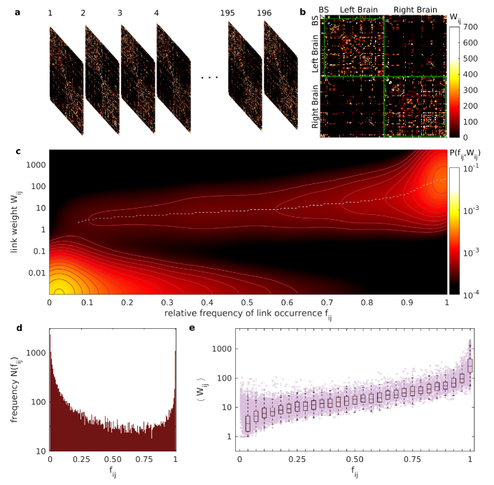
Hence there is no prior reason to expect any correspondence between the ubiquity of a link in the population, as quantified by $f_{ij}$, and the distribution of its weight across the population.

Fig. 1 (c) shows that as the occurrence of links in the population increases, their weights tend to steadily rise, as indicated by the joint probability distribution $P(f_{ij},W_{ij})$ obtained using kernel smoothing (see Methods). The lower plateau represents the links with weight $W_{ij}=0$ and the upper plateau, which includes link weights from $1$ up to order of $1000$, not only displays an increase of $P(f_{ij},W_{ij})$ with increasing occurrence (which trivially leads to increase in non-zero weights), but also shows a steady increase of $W_{ij}$. This indicates that those connections which are found more often in a population are likely to have higher connection weights as well. Fig. 1 (d) displays the frequency histogram of $f_{ij}$ values, showing the highest concentration of links at $0$ and $1$. For a species with rigidly invariant topology over a population, such as C. elegans, this histogram would show occupancy only at $0$ and $1$. Thus a large number of links which occur with frequencies $0$ and $1$ implies high topological variability in the structural connectivity within a population. Even though the distribution of connection weights in the population shows correspondence with the relative frequency of occurrence $f_{ij}$, the distribution widens with an increase in the occurrence. This implies a large variability in connection weights, even for links with similar values of occurrence. Assuming that the processes determining weights are still largely independent of the processes determining the formation of the connection itself (wiring), it is meaningful to consider the weight distribution of non-ubiquitous links ($f_{ij}<1$) over only those individuals from the population in which the link occurs. Fig. 1 (e) shows that even when we consider mean weights of each link ($\langle W_{ij}\rangle$) averaged over the corresponding subset of the population in which the link occurs, there is a steady rise in these partially averaged values of the link weights. This further indicates that wiring and weighting processes for the links are not entirely independent, even if they are separate processes.

The variation of the weights of frequently occurring links over the population, as well as their frequency of occurrence, can both be described by a single link-specific Poisson process.

One of the simplest stochastic processes that describes the distribution of the number of recorded events is the Poisson process. It corresponds to a probability distribution of discrete random independent events occurring at a constant rate over time or space. Here we consider the hypothesis that the link weights $W_{ij}$ for link $(i,j)$ are generated by such discrete independent events occurring at a constant rate $\lambda_{ij}$ for each human subject. In such a case, the link weights $W_{ij}$ would follow a Poisson distribution. As we have already shown above that the processes determining the wiring and the weights of the links appear to be at least mutually dependent, even if they are separate, weights having Poisson distribution would actually mean that a single parameter $\lambda_{ij}$ would be sufficient to explain the variability of link weights as well as their frequency of occurrence.

Figure 2: The variation of the weights of frequently occurring links over the population, as well as their frequency of occurrence, can both be described by a single link-specific Poisson process. (a) Frequency histograms corresponding to four separate links $(i,j)$ demonstrating that their rescaled link weights $\mathcal{W}_{ij}$, obtained using corresponding rescaling factors $s_{ij}$, are distributed over the population in a Poisson process, with respective Poisson parameters $\lambda_{ij}$ displayed in each case. The solid lines, which represent the theoretical values of the distributions, display close agreement with the histograms corresponding to the observed distributions and the shaded region represents the fluctuations in the frequencies over a large number of randomly drawn samples of size $196$ (same as the population size) from the corresponding Poisson distribution. The goodness of fit for the links with the Poisson distribution has been quantitatively tested using Pearson’s Chi-square test Pearson1900 . (b) Scatter plot of the links, represented in terms of their mean weights across entire population $\langle W_{ij}\rangle$ and the their variances $\sigma^{2}_{ij}$. It can be seen that for most links the weight distributions have $\sigma^{2}_{ij}\propto\langle W_{ij}\rangle$, which indicates the possibility of a rescaled Poisson distribution. The links that fit a rescaled Poisson distribution (as shown by Chi-squared goodness of fit test with significance $\alpha=0.01$), are distinguished by showing them in red color and the linear regression fit for those points (red line) has a slope of $1.2$. (c) Links which are shown to fit rescaled Poisson (red dots) have high values for the relative frequency of occurrence ($>0.5$) as well as higher values of mean link weights. (d) Adjacency matrix showing the entries corresponding to $3342$ links that fit the rescaled Poisson distribution with $\alpha=0.01$ (black entries) and $577$ links whose weight distributions deviate from the corresponding Poisson distributions (red entries). (e) Joint probability distribution $P(s_{ij},\lambda_{ij})$ of the distribution of rescaling factors $s_{ij}$ and Poisson parameter $\lambda_{ij}$. We observe that $P(s_{ij},\lambda_{ij})$ is relatively unaffected by increasing or decreasing $\lambda$, which suggests that both these link properties that together determine the observed weights for a link in the population, might originate from distinct biological factors.

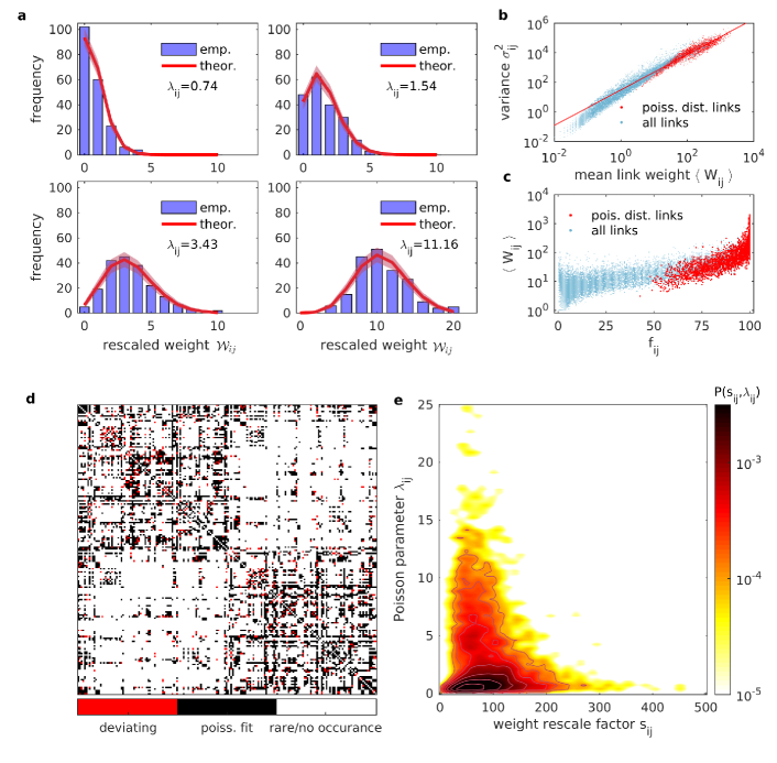
We find that for a large number of frequently occurring links ($f_{ij}>0.5$), their weights follow a rescaled Poisson distribution (see Methods) with each link having specific value of $\lambda_{ij}$ and corresponding rescaling factor $s_{ij}$. The rescaling factor is a link-specific constant scalar value for a link $(i,j)$, which can be applied on its weights $W_{ij}$ across the population to obtain the rescaled weights $\mathcal{W}_{ij}$, which follow a Poisson distribution $\mathcal{P}(\lambda_{ij})$ (see Methods for details). Using Pearson’s Chi-squared goodness of fit test (see Methods) to determine whether the rescaled weights for a link fits a Poisson distribution with high significance ($\alpha=0.01$), we find that out of $15,209$ links that are seen at least once in the population there are $3342$ links whose rescaled link weights can be described by Poisson processes and $11,290$ links have too few occurrences for a reliable statistical fitting. Thus there are only $557$ links that deviate significantly from the Poisson distribution.

Fig. 2 (a) demonstrates that the frequency histogram corresponding to rescaled link weights of four separate links agree with the theoretically expected frequencies from a Poisson distribution having the corresponding $\lambda_{ij}$. As both the mean and variance of Poisson distributions are equal to the same parameter $\lambda$, it is expected that the rescaled Poisson distribution followed by $W_{ij}$ has $\langle W_{ij}\rangle\propto\sigma^{2}_{ij}$, as can be seen in Fig. 2 (b). Fig. 2 (c) shows that links described by a Poisson process appear to have high significance in the structural connectivity in terms of both the topology (by having higher values of $f_{ij}$), as well as, the strength of connection (by having higher values of partially averaged mean link weights as described in Fig. 1 (e)). The adjacency matrix in Fig. 2 (d) illustrates the highly dense network comprising of links described by Poisson processes, while also showing the sparsely distributed $557$ links that deviate from the Poisson process. Further, the two factors determining the connection weight for a link, viz. $\lambda_{ij}$ and $s_{ij}$, seem to have no dependence on each other, as can be seen in their joint probability distribution in Fig. 2 (e). The Pearson’s correlation coefficient between respective values of $\lambda_{ij}$ and $s_{ij}$ is $-0.09$.

Figure 3: Exclusion of a small fraction of outliers can make deviating links fit a Poisson distribution. (a) Frequency histograms corresponding to four separate links $(i,j)$ demonstrating that rescaled link weights $\mathcal{W}_{ij}$ obtained using corresponding rescaling factors $s_{ij}$ are distributed over the bulk of the population in a Poisson process (represented by blue bars), upon excluding a few outliers ($<10\%$ of the population, represented by red bars) with high values that deviate from the Poisson process. The solid lines which represent the theoretical values of the distributions display close agreement with the histograms corresponding to the observed distributions for the bulk of the population (blue bars) and the shaded region represents the variability in the frequencies across a large number of randomly drawn samples of size $196$ (same as the population size) from the corresponding Poisson distribution. (b) Adjacency matrix showing that $520$ links (shown as black entries) out of the $577$ links that originally deviated from the Poisson distribution over the entire population (as shown in Fig. 2 (d)), fit the Poisson distribution on removing only upto $10\%$ outliers from the population, as quantitatively shown using the Chi-squared test. The remaining $57$ links do not fit a Poisson distribution even after the removal of $10\%$ outliers (shown as red entries). (c) The empirically observed fraction of links whose weights deviate from the Poisson distribution $f_{dev}$ (out of all the links with sufficient frequency of occurrence, viz.$\approx 0.15$, as indicated by the arrow), cannot be explained by finite size effect alone. The probability distribution shows the expected values for $f_{dev}$ in a randomly generated network ensemble of sample size $196$, where each link weight across all the networks is drawn from a Poisson distribution with link-specific values of $\lambda_{ij}$ that were obtained from the empirical dataset. Finite size effects contribute a value of $f_{dev}\approx 0.03$ which is much smaller than that observed from empirical data.

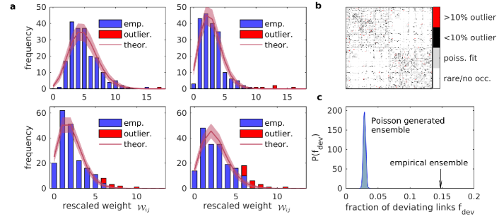
We next examine the $577$ links which, in spite of having high frequency of occurrence, do not fit Poisson distribution. We observed that the bulk of these links have a bimodal distribution of rescaled weights, in which the first mode appears to be a Poisson distribution while the other mode (occurring at much higher values) comprises outliers with unexpectedly high weights. Hence the deviation from a purely Poisson process can possibly be attributed to such outliers. The rescaling factor $s_{ij}$ and Poisson parameter $\lambda_{ij}$ obtained from these links are possibly inaccurate because they are calculated by including the outlier values. Thus, for each of these deviating links, we sequentially remove the data points with the largest weight, calculate the $\lambda_{ij}$ and $s_{ij}$ for the remaining subset and rescaling the weights until the remaining data agrees with the Poisson process as per Chi-squared goodness of fit with a high significance ($\alpha=0.01$). Out of $577$ deviating links, we find that $520$ links fit the rescaled Poisson distribution after excluding less than $10\%$ of the outliers. Fig. 3 (a) demonstrates that in four of the deviating links that are shown, the bulk of the distribution ($>90\%$) agrees with a Poisson distribution, while the outliers ($<10\%$) deviate significantly from the theoretical distribution. The adjacency matrix in Fig. 3 (b) shows that the bulk of the deviating links fit the Poisson distribution by excluding few outliers. We note that out of a total of $3919$ links that have sufficient occurrences for statistical tests, $3862$ links ($98.5\%$) have their weights distributed according to link specific Poisson processes for more than $90\%$ of the population.

The deviation observed in these $577$ links suggests that even though a single Poisson process might be sufficient to describe the wiring and the weights for a large fraction of links for most of the population, there may be other factors in the generative mechanism that lead to a significant fraction of links ($\approx 0.15$) deviating from a Poisson process, even if that deviation is due to the presence of a few outliers within the population. In order to rule out the possibility that the deviation arises simply because of finite size effects in the specific distribution of $\lambda$ values, we generated a surrogate ensemble of SC matrix sets, each comprising $196$ matrices. The link weights were each drawn from the link-specific Poisson distributions (see Methods for details). We find that in every realization, a small fraction of links does not fit a Poisson distribution, as per the Chi-squared criterion. The distribution of these values is shown in Fig. 3 (c). The deviations arising due to such finite size effects are significantly lower than those seen empirically. This suggests that there must be other significant factors in the generative mechanisms apart from the Poisson process that give rise to the structural connectivity in human brains.

Rescaling of link weights using Poisson parameters might provide greater functional interpretability to the structural connectivity.

While we have have thus far interpreted the Poisson parameter $\lambda_{ij}$ for the links as an abstract representation of the net effect of all biological factors associated with the generative mechanism of the structural connectivity of brain networks, an additional interpretation of the Poisson parameter can be obtained by considering its effect on function. While there have been several attempts to examine the relation between structural connectivity and functional connectivity Honey2009 ; Hagmann2008 , it has been observed that there is very low correspondence between the two. Unlike synaptic and gap-junction weights which are interpreted as coupling strengths between neuronal activities, the connection weights in the structural macro-connectome elude a functional interpretation (such as for instance being a measure of dynamical coupling between the activities of different brain regions). We have already observed that rescaled weights appear to be a more fundamental structural property than the original weights, since they are essentially discrete Poisson variables which are known to arise in a wide range of natural phenomena. It is therefore reasonable to ask whether the rescaled weights can have a deeper relation with the functional coupling. For example, could the rescaled weight be directly related to the number of axons in axonal tracts? Here we ask whether the individual structural connectivity of rescaled weights, which are obtained from the analysis of SC matrices across a population, have a stronger correlation with the corresponding functional connectivity as compared to the original structural connectivity.

The Nathan Kline Institute (NKI) / Rockland Sample dataset that we consider Nooner2012 includes resting state functional connectivities (FC) for each of the $196$ individuals whose structural connectivity we have analyzed thus far. Sample functional connectivity matrices are displayed in Fig. 4 (a). In contrast to the structural connectivities, the functional connectivities exhibit a large degree of variability across individuals. Examining a single FC matrix (Fig. 4 (b)) reveals that the density of strong functional connections is much higher than that of structural connections (Fig. 1 (b)), and unlike the structural networks there is a significant number of connections across left and right hemispheres. We first examine the correlation between the structural and functional connection strengths for each link ($W_{ij}$ and $C_{ij}$, respectively) over the entire population and observe that most of the links have negligible correlation between the variations of structural and functional connectivity strengths over the population (see Fig. S1 in SI). While this supports the previously known observation that there is very low correspondence between structure and function at the level of individual links, we observe that a macroscopic comparison between the FC matrices ($C_{(n)}$) and structural weight matrices ($W_{(n)}$) for each individual $n$ reveals statistically significant correlations, as seen in Fig. 4 (c). Furthermore, for every individual in the population we observe that the matrix correlation of $C_{(n)}$ and structural weight matrix $W_{(n)}$ is lower than the matrix correlation of $C_{(n)}$ and the corresponding rescaled structural weight matrix $\mathcal{W}_{(n)}$. Thus, there is a notable correspondence between

Figure 4: Upon rescaling the weights, the structural connectivities consistently show a greater association with the corresponding functional connectivities across the population. (a) Ensemble of functional connectivity (FC) matrices representing the resting state functional brain networks, determined by functional magnetic resonance imaging (fMRI), of the same $196$ human subjects whose structural connectivities have been analyzed in this work. (b) A sample FC matrix corresponding to one of the subjects. The nodes are arranged in the same way as described in Fig. 1 (b), and the matrix entries $C_{ij}$ indicate the correlation between the haemodynamic activities of nodes $i$ and $j$ over a period of time. Notice the striking difference between the SC shown in Fig. 1 (b) and the FC shown here. Where the SC have relatively sparse connections and a much higher density of ipsilateral connections than the contralateral ones, the FC have a much higher density of strong connections (both positive and negative) with equal density of functional connectivity between ipsilateral (diagonal blocks) as well as between contralateral regions (off diagonal blocks). (c) A comparison of the dependence between individual functional connectivity matrices ($C_{(n)}$) for an individual $n$ (where $n\in{1,2,3\ldots 196}$) and the corresponding structural connectivities described respectively by weight matrices ($W_{(n)}$) and rescaled weight matrices ($\mathcal{W}_{(n)}$). Examples of the three types of matrices are shown as insets. The scatter plot displays the correlation between $C_{(n)}$ and $W_{(n)}$ for each $n$ along the x-axis, and the corresponding correlation between $C_{(n)}$ and $\mathcal{W}_{(n)}$ along the y-axis. Note that while the correlations between functional and structural matrices of both types are very low ($<0.3$) (even though statistically significant), for every individual in the population the functional connectivity matrices are more correlated with the corresponding $\mathcal{W}_{(n)}$ than they are with $W_{(n)}$. (d) Box-plots representing the distributions of the correlations of the functional matrix $C_{(n)}$ for each individual $n$ with the corresponding matrices weight $W_{(n)}$ and $\mathcal{W}_{(n)}$ and the adjacency matrix $\mathcal{A}_{(n)}$, generated from the rescaled weight matrix $\mathcal{W}_{(n)}$ by removing information about the link weights. The correlation distribution for $\mathcal{W}_{(n)}$ which is positioned higher than that corresponding to $W_{(n)}$ as expected from the result in panel (c), is higher compared to the correlation distribution for $\mathcal{A}_{(n)}$, which contains information related to the topology of the rescaled matrix but not the link weights. Note that topology of the rescaled weight matrices are different from that of the original weight matrices, since the former has much fewer links. This implies that in addition to the altered topology of rescaled weight matrices, the altered weight distribution also makes $\mathcal{W}_{(n)}$ a better structural correlate of the observed dynamical function of the brain.

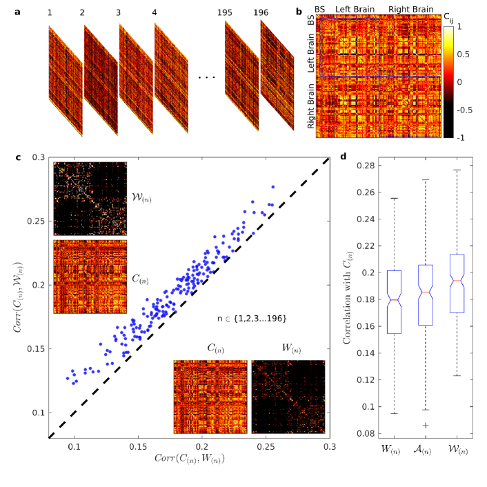
structure and function for each individual at the level of the entire brain network, and furthermore, the rescaling of weights in the structural connectivity enhances this correspondence between structure and function in all individuals. A possible explanation for this enhanced correspondence with function might be the alteration in the distribution of weights after rescaling, or it might also be attributed to the change in the connection topology due to the rescaling of weights (as the rescaling process leads to the deletion of links). To examine this, we computed matrix correlations of each $C_{(n)}$ with (unweighted) adjacency matrices having the same connectivity as $\mathcal{W}_{(n)}$, which we refer to as $\mathcal{A}_{(n)}$. The boxplots in Fig. 4 (d) shows that the matrix correlations of $C_{(n)}$ with $\mathcal{W}_{(n)}$ are higher than correlations with $\mathcal{A}_{(n)}$, suggesting that the alteration of the weight distribution upon rescaling is the primary factor in making SC a better correlate of FC. The three distributions of matrix correlation values were found to be significantly distinct from one another using the Two-sample Kolmogorov-Smirnov (KS) test (see Methods).

The resting state functional connectivities of the individuals in the dataset are simplified snapshots of a large repertoire of complex dynamical behaviors in the brain, which are associated with various cognitive functions and arise from highly complex non-linear interactions among the constituent brain regions. Therefore a simple correspondence between structural and functional connectivities would not be sufficient to establish that a rescaled weight distribution in structural connectivity would be a better functional correlate than the original weight distribution. In order to understand how the weights in the structural connectivity affect the dynamics, we simulate the complex dynamical activity that would arise when the structural connectivity provides the basis for the non-linear interactions between the brain regions. To describe the dynamical activity of brain regions, we use a well-known neural mass model, viz., the Wilson-Cowan (WC) model Wilson1972 ; Destexhe2009 (see Methods for details). Fig. 5 (a) shows a schematic representation of one WC node which is used to represent the activity in a single brain region. In order to generate the time series of simulated activity of all brain region for each individual, we simulated systems of WC oscillators placed at the nodes of networks with the corresponding structural connectivity matrix ($W_{ij}$, as well as, $\mathcal{W}_{ij}$), with the associated connection strengths of these matrices taken to be the same as the dynamical coupling strengths $w_{ij}$ between WC nodes. Fig. 5 (b) shows samples of such time series. By computing Pearson’s correlation coefficient between the time series of activity for each pair of brain regions, we generated the simulated functional connectivity matrices $C^{W}$ (Fig. 5 (c)) and $C^{\mathcal{W}}$ (Fig. 5 (d)) for each individual to compare with the corresponding empirical functional matrices $C$ (Fig. 5 (e)). We compared the matrix correlations between individual $C_{(n)}$ and $C^{\mathcal{W}}_{(n)}$ with correlations between individual $C_{(n)}$ and $C^{W}_{(n)}$ matrices, as shown in Fig. 5 (f). Similar to the result obtained from the comparison of FC matrices with SC matrices in Fig. 4 (c), we find that simulated FC generated from rescaled weight matrices $\mathcal{W}_{(n)}$ were consistently better correlated with empirical FC than the ones generated from original

Figure 5: Dynamical simulation of whole brain activity using a neuronal population model suggests that structural connectivity with rescaled weights are better structural correlates for brain function than those with original weights. (a) Schematic representation of a single dynamical element (oscillator) of the Wilson-Cowan (WC) model, which simulates the activity within a single region of the brain network, each comprising interactions between the excitatory and inhibitory subpopulations ($U$ and $V$ respectively), with strengths denoted by $c_{\mu\nu}$ where $\mu,\nu=\{u,v\}$, and their interactions with the subpopulations belonging to other nodes of the network (with uniform coupling strength $w$). The lightning bolt represents the external stimulation of strength $I_{u}$ provided to the excitatory subpopulation. (b) Time evolution of the dynamical activity of the excitatory subpopulations in four out of $188$ brain regions of a single individual, obtained from simulations of WC oscillators on the network specified by the structural connectivity matrix associated with the rescaled weights $\mathcal{W}$ as coupling strengths. As the model is dimensionless, here time is displayed in arbitrary units (a.u.). (c-d) Functional connectivity matrices obtained from simulated brain activity using one of the connectomes. The matrices $C^{W}$ and $C^{\mathcal{W}}$ are respectively obtained from simulations of WC oscillators on (c) the original weight matrix $W$, and (d) the rescaled weight matrix $\mathcal{W}$. (e) Empirical functional connectivity obtained from the resting state brain activity of the same individual. (f) Scatter plot displaying the correlation between the empirical FC matrices $C_{(n)}$ and the simulated FC matrices obtained from the original weight matrices $C^{W}_{(n)}$ for each individual $n$ along the abscissa, and the correlation between $C_{(n)}$ and the simulated FC matrix obtained from rescaled weight matrix $C^{\mathcal{W}}_{(n)}$ along the ordinate. It can be observed that $corr(C_{(n)},C^{\mathcal{W}}_{(n)})$ is consistently higher than $corr(C_{(n)},C^{W}_{(n)})$ for the majority of individuals. This further extends the result shown in Fig. 4 (c). (g) Box-plot showing that the correlations of the empirical FC of individual brains $C_{(n)}$ with simulated FC from corresponding rescaled weight matrices $C^{\mathcal{W}}_{(n)}$ are comparatively higher than both $corr(C_{(n)},C^{W}_{(n)})$ and $corr(C_{(n)},C^{\mathcal{A}_{(n)}})$, where $C^{W}_{(n)}$ represents the simulated FC matrices obtained from corresponding weight matrices, and $C^{\mathcal{A}}_{(n)}$ represents the corresponding adjacency matrices of the rescaled weights. Furthermore, as $corr(C_{(n)},C^{\mathcal{A}_{(n)}})$ is the weakest, it suggests that the dynamical behavior of the brain is governed more strongly by the weight distribution of the structural connectivity than by the network topology. We also obtain simulated FC generated from two alternative representative structural networks of a human brain, viz. $C^{\langle W\rangle}$ which is generated from the matrix $\langle W\rangle$ that we obtain by averaging each link weight $W_{ij}$ over entire population and $C^{\lambda}$ which is generated from the matrix $\lambda$, which comprises the Poisson parameters $\lambda_{ij}$ for each link that is Poisson distributed over at least $90\%$ of the population. We observe that the empirical FC matrices correlate better with the simulated FC $C^{\lambda}$ compared to the simulated FC $C^{\langle W\rangle}$, as indicated by the box-plots.

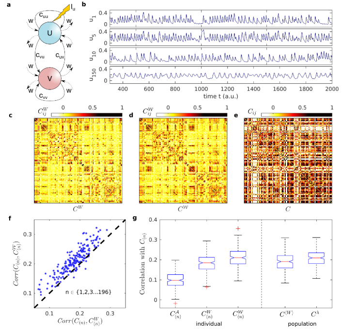
weight matrices $W_{(n)}$. We also generated simulated FC from adjacency matrices $\mathcal{A}_{(n)}$ obtained from $\mathcal{W}_{(n)}$ and found that FC generated from adjacency matrices had the weakest correlation with the empirical matrices out of all three types of simulated FC, as seen in first three box-plots in Fig. 5 (g). This strongly suggests that the dynamics in complex non-linear systems such as the brain is governed much more strongly by the weight distributions of the connectivity than the connection topology itself.

Finally, we compare each of the empirical FC with the corresponding matrix generated by a generic “representative” network that would describe the structural connectivity of the human brain. There are two alternative ways to obtain a “representative” network from the SC ensemble. The widely used approach is to obtain an average network $\langle W\rangle$, which comprises the average weight of each link calculated over entire population. Our results suggest a second approach, which is to consider the $\lambda$ matrix, comprising the Poisson parameters $\lambda_{ij}$ for all the Poisson distributed links, as the representative network. By construction, it comprises only those links that follow a Poisson distribution. As we have already observed that rescaled weights of an individual SC might be more relevant in interpreting structural connections, it is more meaningful to consider the $\Lambda$ matrix (which effectively is the average of all rescaled weight matrices), as the representative structural network. We generate simulated FCs corresponding to $\langle W\rangle$ and $\Lambda$, and observe that FC generated from $\Lambda$ is more strongly correlated with the bulk of the empirical FCs than the one generated form $\langle W\rangle$, as seen in the last two box-plots of Fig. 5 (g). All the correlation distributions being considered here have been shown to be significantly distinct from each other using the Two-sample Kolmogorov-Smirnov (KS) test (see Methods).

The representative structural connectome can be resolved into two components: “Basal” network and “Superstructure” network.

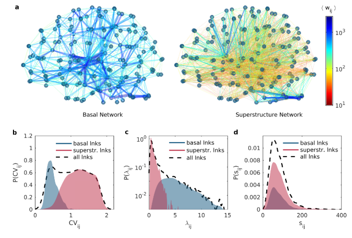
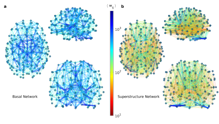
We have thus far argued that the representative network described by the $\Lambda$ matrix is significant because: (i) the underlying generative mechanisms for determining the wiring and weighting of links can be described by a Poisson process (Fig. 2 and Fig. 3), (ii) the constituent links are significant in terms of topology, as well as, connection weights (Fig. 2 (c)), and (iii) The $\Lambda$ matrix is a better structural correlate to observed function in comparison to the average SC matrix. We now return to one of our original questions regarding the extent of variability of the structural network within the population in terms of topology and weight distribution, focusing only on the constituent links of the representative network. On examining how various link-specific properties, such as the coefficient of variation of link weights ($CV_{ij}$) and Poisson parameters ($\lambda_{ij}$) are distributed among the constituent links of the representative network, we find that the network can be resolved into two distinct classes of links that we refer to as the “basal” and the “superstructure” network, shown in Fig. 6 (a). The former comprises links that are seen in all individuals ($f_{ij}=1$) while the latter contains all the remaining links of the representative network. They can be identified from the clearly observable bimodality in the distributions of $CV_{ij}$ (Fig. 6 (b)) and $\lambda_{ij}$ (Fig. 6 (c)). The bimodality in both distributions can be verified by calculating their bimodality coefficients (see Methods). Basal links are distinguished by very low variability in weight across the population but high values of average weights and $\lambda_{ij}$, while the superstructure links show highly variable connection weights across the population, but typically low values of average link weights and $\lambda_{ij}$. Notably, the distribution of weight rescaling factors $s_{ij}$ does not show any distinction between the basal and superstructure networks (Fig. 6 (d)). Planar projections of the basal and superstructure networks on horizontal, sagittal and coronal planes are provided in Fig. 7.

Using the representative network for human brain as the basis, we can explore the mesoscopic organization of human brain in the same way as was done for macaque brain in Pathak2020 . We have shown the preliminary results from our modular analysis of human brain network in SI.

Figure 6: The representative structural connectivity of a brain network can be resolved into two components. (a) Sagittal plane projections of the “basal” network (left) and the “superstructure” network (right). The former comprises $1106$ ubiquitous links, i.e., those that occur in every individual, and the latter consists of the remaining $2806$ links. The thickness and color of each link between a pair of regions $(i,j)$ corresponds to their average weights $\langle w_{ij}\rangle$ across the population (see legend). Note that the average link weights in the basal networks are much higher than those in the superstructure network. (b) The distribution of the coefficients of variation $CV_{ij}$ for the link weights across the population (indicated by broken lines) is observed to be bimodal. The mode corresponding to lower values of $CV_{ij}$ is attributed to links from the basal network (blue shaded region), whereas the links from the superstructure network (red shaded region) primarily contribute to the mode corresponding to higher values of $CV_{ij}$. This demonstrates that the links of the basal network tend to have higher link weights on an average, and their weights are largely invariant across the population. In contrast, the link weights in the superstructure network vary across individuals. (c) The distribution of Poisson parameters $\lambda_{ij}$ (indicated by broken lines) is also bimodal, with each mode corresponding to the basal network links (blue shaded region) and superstructure links (red shaded region) respectively. (d) The distribution of weight rescaling factors $s_{ij}$ (broken lines) is observed to be unimodal, in contrast to $\lambda_{ij}$ and $CV_{ij}$, with no distinction between the basal and the superstructure links as indicated by their strongly overlapping distributions (blue and red shaded regions). Note that the separate distributions for basal network links and superstructure network links are normalized according to their relative sizes.

Figure 7: “Basal” network and “Superstructure” Network. (a) Horizontal, sagittal and coronal projections of the spatial representations for the “basal” network (left, top right and bottom right respectively). (b) Horizontal, sagittal and coronal projections of the spatial representations for the “superstructure” network (left, top right and bottom right respectively). Note that the average weights $\langle w_{ij}\rangle$ (represented by the thickness and color of the links $(i,j)$, see legend) display a smooth spatial gradient. In addition, the long range connections between spatially distant regions are more frequently observed in the superstructure network, as compared to the basal network whose structure is closer to a lattice in that most of the connections are between spatially adjacent regions.

IV Discussion

Our results suggest that the expected weight distribution of a link in the structural connectome, as well as its expected probability of occurrence in an individual, can be described by a single parameter. This is indicative of a common generative mechanism that determines both the connection topology of the axonal tract wiring between brain regions, as well as, the anatomical thickness of the tracts, which we refer to as the connection weight. At the neuronal scale connection weights refer to the number of synapses between two neurons, or the synaptic conductivity. These quantities have a direct measurable effect on the complex electrophysiological interactions between the neurons. The plasticity and learning mechanisms that determine and alter the connection weights between neurons are well understood, e.g., spike-time dependent plasticity. However, in the case of the macro-connectome, the role of connection weights, viz., the density of axonal bundles, in the functional interactions of the brain areas is not well understood. By determining a latent Poisson distributed quantity from the observed weight of a connection, which we refer to as the rescaled weight, our results point towards a potential framework for a better functional interpretation of structural connectivity. This might be extremely useful in the development of dynamical models of various cognitive phenomena in the brain. To probe this, we have used a relatively simple neural mass model to show that the rescaled weights consistently give rise to dynamical behavior that have better correspondence with the empirical data. This mode of functional interpretation of structural connectivity can be further enhanced when we also consider information related to whether the synaptic connections underlying given axonal pathways are excitatory, inhibitory or both. Another component that is missing from the analysis of structural connectome is the directional information about the connections. Although we represent the structural connectome as an undirected weighted network, in reality synaptic connections are always directed. The observation that the rescaled weight distribution showed a widespread enhancement in correspondence between structure and function, even without the associated information about the directionality and the type of connections, underpins the significance of this framework. In that case, the latent Poisson parameter associated with the axonal pathway, i.e., the rescaled weight, might represent functionally relevant factors such as the actual number of axons in the tract or the number of synaptic connections, rather than simply representing the anatomical thickness. Similarly, the corresponding rescaling factors might be representative of peripheral features that do not directly affect the neuronal interactions, e.g., the thickness of myelin sheaths covering the axons.

We further observe that a significant fraction of links showed deviations from a Poisson generative process, and these deviations are far greater than expected by the finite size of the data. This further illuminates the generative mechanism: even though random independent discrete processes might be involved in the wiring of major portion of the brain, as indicated by the occurrence of Poisson distributions, there are other significant effects at play. These might arise from genetic or developmental factors, or may be governed by the specific functioning of an individual brain. For instance, pathways between certain motor regions in the brain of a professional athlete might be exceptionally stronger than that of other individuals due to prolonged specialized usage of certain circuits. Thus the deviations might be indicative of plasticity in the macro-connectome - a hypothesis that requires further exploration.

In this study we have argued that the inclusion of only the Poisson-distributed links in a generic representative network for a human connectome, with the corresponding weights being the link specific Poisson parameters, is a more meaningful approach than simply obtaining an average of all structural connectivity matrices. The representative network based on Poisson parameters at once informs us about the topological significance, the extent of variability, the generative mechanism and the functional importance of the underlying links, thus making it far more useful for further network-theoretic or dynamical analysis. The two distinct components of the representative network, which we refer as the basal and the superstructure networks respectively, reveal an altogether new organizational aspect of the brain. While the source of this dichotomy within the structural connectome is not clear, one needs to do a more detailed exploration into the developmental and functional implications of the two clearly distinguished components that comprise a generic representative structural connectome of a human brain.

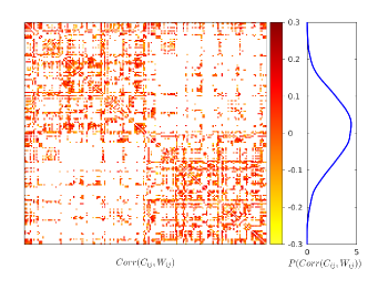
Structure-function correlation for each link

In Fig. S1, we display the correspondence between structure and function for every link $(i,j)$ belonging to the “representative” brain network over the population of individuals (see main text). We observe that the link-wise correlation $Corr(W_{ij},C_{ij})$ between the structural connection weights $W_{ij}$ and corresponding weights in functional connectivities $C_{ij}$, calculated across all individuals, tends to be extremely low for most of the links. This suggests that the functional connectivity has a negligible dependence on the structural connectivity when observed at the level of nodes and links. This is in contrast with the macro-level picture shown in Fig. 4 of main text, where we compared the structural and functional connectivities across entire networks, and found a comparatively higher and statistically significant correspondence between the two.

Figure S1: The link-wise correlations between each structural connection and its corresponding functional connection over the population are extremely low. For each link between a pair of regions $(i,j)$ we display the correlation between their structural connection weights $W_{ij}$ and corresponding weights in functional connectivities $C_{ij}$, calculated across all individuals (left panel). The probability distributions for the correlation values are shown in the right panel. Only those links that are identified as part of the representative network, i.e., whose weights are Poisson distributed over the population, are shown here.

Community structure in the human structural connectome

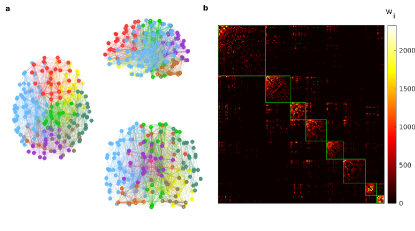
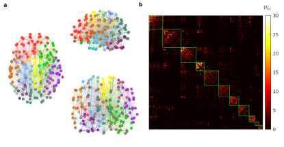
We have analyzed two types structural connectivity: the first corresponding to original connection weights, as given in the database, and the second consisting of “rescaled” connection weights (for details, see Methods). We have found modules in the brain network of each individual by implementing two separate community detection methods which are described in Pathak2020 , viz., Newman Spectral Analysis Newman2006 and the Infomap Method Rosvall2008 . We have included only those links that comprise the “representative” structural network (as described in the main text). Fig. S2 and S3 show the modular decomposition of the original network (Fig. S2) and the rescaled network (Fig. S3) for the same individual, as obtained from Newman Spectral Analysis.

Figure S2: Modules in the structural brain network of an individual subject, obtained using Newman Spectral Analysis. (a) Horizontal, sagittal and coronal projections (left, top right and bottom right, respectively) of the spatial representations for the structural brain network of an individual subject, highlighting the $6$ modules obtained from Newman Spectral Analysis. Here, the nodes are colored in accordance with the module to which they belong, and the color of each link corresponds to that of its respective source node, while the thickness of each links is proportional to its connection weight. Only those links that are part of the representative network (as described in the main text) are considered here. (b) Weighted adjacency matrix representing the network shown in panel (a). Here, the nodes are rearranged and grouped according to their modular membership. The matrix elements are colored in accordance with the connection weights $W_{ij}$ of the corresponding links (see legend at the right). The $6$ modules that were obtained from the analysis correspond to the diagonal blocks, marked by green lines.

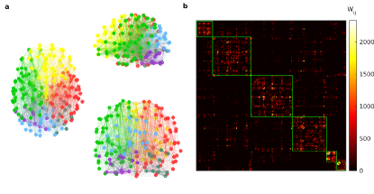
We observe that the modules obtained are spatially contiguous with clearly defined boundaries. There is only a slight variation between the modular partitionings of the two types of the networks shown in Fig. S2 and S3. The similarity of modular partitioning between different individuals is shown in Fig. S4 where we show the normalized mutual information $I_{norm}$ between all pairs of modular partitionings (for details about normalized mutual information, see Pathak2020 ). For most pairs of individuals, the $I_{norm}$ values are $\approx 0.5$, which indicates that modular partitioning is moderately varying across individuals.

Figure S3: Modules in the rescaled structural brain network of an individual subject, obtained using the Newman Spectral Analysis. (a) Horizontal, sagittal and coronal projections (left, top, right and bottom right, respectively) of the spatial representations for the rescaled structural brain network of an individual subject, highlighting the $6$ modules obtained from Newman Spectral Analysis. The individual represented here is the same as that in Fig. S2. Here, the nodes are colored in accordance with the module to which they belong, and the color of each link corresponds to that of its respective source node, while the thickness of each links is proportional to its connection weight. Only those links that are part of the representative network (as described in the main text) are considered here. (b) Weighted adjacency matrix representing the rescaled network shown in panel (a). Here, the nodes are rearranged and grouped according to their modular membership. The matrix elements are colored in accordance with the rescaled connection weights $\mathcal{W}_{ij}$ of the corresponding links (see legend at the right). The $6$ modules that were obtained from the analysis correspond to the diagonal blocks, marked by green lines.

Figure S4: Similarity of Newman Spectral modules across different individual brain networks. Pair-wise values of $I_{norm}$, which quantifies the similarity of modular paritionings between a pair of individuals, as well as the kernel-smoothened distributions of the corresponding $I_{norm}$ values, are shown for (a) the brain networks having original connection weights, and (b) brain networks having rescaled weights. Note that the mode of the $I_{norm}$ distributions in both cases is $\approx 0.5$, indicating that the modular decomposition of individual brain networks varies moderately over the population.

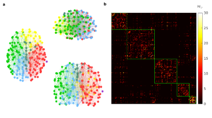
Qualitatively similar results are obtained on using the Infomap method to detect modules in original structural network (Fig. S5) and the rescaled structural network (Fig. S6). The networks represented in Fig. S5 and S6 are from the same individual as that in Fig. S2 and S3. Fig. S7 shows that the modules obtained across the individuals using Infomap method are relatively more similar to each other, as indicated by higher $I_{norm}$ values, in comparison to those obtained using Newman Spectral Analysis.

Figure S5: Modules in the structural brain network of an individual subject, obtained using the Infomap method. (a) Horizontal, sagittal and coronal projections (left, top, right and bottom right, respectively) of the spatial representations for the structural brain network of an individual subject, highlighting the $8$ modules obtained from the Infomap method. The individual represented here is the same as that in Fig. S2. Here, the nodes are colored in accordance with the module to which they belong, and the color of each link corresponds to that of its respective source node, while the thickness of each link is proportional to its connection weight. Only those links that are part of the representative network (as described in the main text) are considered here. (b) Weighted adjacency matrix representing the network shown in panel (a). Here, the nodes are rearranged and grouped according to their modular membership. The matrix elements are colored in accordance with the connection weights $W_{ij}$ of the corresponding links (see legend at the right). The $8$ modules that were obtained from the analysis correspond to the diagonal blocks, marked by green lines.

Figure S6: Modules in the rescaled structural brain network of an individual subject, obtained using the Infomap method. (a) Horizontal, sagittal and coronal projections (left, top, right and bottom right, respectively) of the spatial representations for the rescaled structural brain network of an individual subject, highlighting the $11$ modules obtained from the Infomap method. The individual represented here is the same as that in Fig. S2. Here, the nodes are colored in accordance with the module to which they belong, and the color of each link corresponds to that of its respective source node, while the thickness of each link is proportional to its connection weight. Only those links that are part of the representative network (as described in the main text) are considered here. (b) Weighted adjacency matrix representing the rescaled network shown in panel (a). Here, the nodes are rearranged and grouped according to their modular membership. The matrix elements are colored in accordance with the rescaled connection weights $\mathcal{W}_{ij}$ of the corresponding links (see legend at the right). The $11$ modules that were obtained from the analysis correspond to the diagonal blocks, marked by green lines.

Figure S7: Similarity of Infomap modules across different individual brain networks. Pair-wise values of $I_{norm}$, which quantifies the similarity of modular paritionings between a pair of individuals, as well as the kernel-smoothened distributions of the corresponding $I_{norm}$ values, are shown for (a) the brain networks having original connection weights, and (b) brain networks having rescaled weights. Note that the mode of the $I_{norm}$ distributions in both cases is $\approx 0.6$, indicating that the modular decomposition of individual brain networks varies moderately over the population.