Self-dual criticality in three-dimensional $\mathbb{Z}_{2}$ gauge theory with matter

Abstract

The simplest topologically ordered phase in 2+1D is the deconfined phase of $\mathbb{Z}_{2}$ gauge theory, realized for example in the toric code. This phase permits a duality that exchanges electric and magnetic excitations (“$e$” and “$m$” particles). Condensing either particle while the other remains gapped yields a phase transition with 3D Ising exponents. More mysterious, however, is the transition out of the deconfined phase when self-duality symmetry is preserved. If this transition is continuous, which has so far been unclear, then it may be the simplest critical point for which we still lack any useful continuum Lagrangian description. This transition also has a soft matter interpretation, as a multicritical point for classical membranes in 3D.

We study the self-dual transition with Monte Carlo simulations of the $\mathbb{Z}_{2}$ gauge-Higgs model on cubic lattices of linear size $L\leq 96$. Our results indicate a continuous transition: for example, cumulants show a striking parameter-free scaling collapse. We estimate scaling dimensions by using duality symmetry to distinguish the leading duality-odd/duality-even scaling operators $A$ and $S$. All local operators have large scaling dimensions, making standard techniques for locating the critical point ineffective. We develop an alternative using “renormalization group trajectories” of cumulants. We check that two- and three-point functions, and temporal correlators in the Monte-Carlo dynamics, are scale-invariant, with scaling dimensions $x_{A}$ and $x_{S}$ and dynamical exponent $z$.

We also give a picture for emergence of 1-form symmetries, in some parts of the phase diagram, in terms of “patching” of membranes/worldsurfaces. We relate this to the percolation of anyon worldlines in spacetime. Analyzing percolation yields a fourth exponent for the self-dual transition. We propose variations of the model for further investigation.

I Introduction

Continuum field theory provides a language for a huge range of classical and quantum phase transitions Fisher (1974); Sachdev (2007). This includes many cases for which a simple Landau-Ginsburg formulation is insufficient Wegner (1971); Kosterlitz and Thouless (1973); de Gennes (1972); Huse and Leibler (1991); Lammert et al. (1993); Francesco et al. (2012); Fradkin (2013); Senthil et al. (2004). For example, a wide range of topological phase transitions, lacking any local order parameter Wegner (1971), may be brought under some measure of analytical control using the language of continuum gauge theory, together with various kinds of perturbative expansion ($\epsilon$ expansions, large $N$ expansions, etcetera). However, despite the wild success of the field theory approach to critical phenomena, there exist phase transitions in simple and natural models that still remain out of reach of field theory tools. This paper characterizes what we suggest is the paradigmatic example of these mysterious transitions. This is the “self-dual” phase transition between confined and deconfined phases of $\mathbb{Z}_{2}$ gauge theory in three dimensions Fradkin and Shenker (1979); Jongeward et al. (1980); Tupitsyn et al. (2010); Vidal et al. (2009).

The $\mathbb{Z}_{2}$ gauge–Higgs model Wegner (1971); Kogut (1979); Fradkin and Shenker (1979) has a stable deconfined phase, as well as a trivial phase, in three dimensions. In the context of quantum systems in 2+1D (the model also has a 3D classical interpretation that we discuss below) the deconfined phase is the simplest $\mathbb{Z}_{2}$ spin liquid Read and Chakraborty (1989); Kivelson (1989); Read and Sachdev (1991); Wen (1991); Senthil and Fisher (2000); Moessner et al. (2001): the phase of matter realized, for example, by the toric code Kitaev (2003). The anyon excitations of this phase include quasiparticles denoted $e$ and $m$, with nontrivial mutual statistics, which correspond to charge and flux in the gauge theory.

The simplest lattice field theory formulation of the $\mathbb{Z}_{2}$ gauge-Higgs model has a two-dimensional parameter space Wegner (1971); Balian et al. (1974); Kogut (1979); Fradkin and Shenker (1979); Jongeward et al. (1980); Tupitsyn et al. (2010). In the quantum language, these two couplings allow us to separately control the masses of both $e$ and $m$ excitations. In the language of the lattice gauge theory, one of the couplings controls the “stiffness” associated with fluctuations of the matter field, and the other the stiffness of gauge field: see the schematic Fig. 1.

While there are only two stable phases in Fig. 1, there are various possibilities for the transition between them Fradkin and Shenker (1979); Jongeward et al. (1980); Huse and Leibler (1991); Vidal et al. (2009); Tupitsyn et al. (2010). The Higgs and confinement transitions correspond to condensation of the $e$ particle, and of the $m$ particle, respectively. These two lines of transitions are in fact completely equivalent, as they are mapped into each other by the crucial duality transformation, which exchanges the two kinds of particle. They are subtle phase transitions with no local order parameter Wegner (1971). Nevertheless, they are amenable to field theory tools. For example, gauge fluctuations are in fact irrelevant at the Higgs transition Fradkin and Shenker (1979). Its universal scaling is therefore same as in the limit of infinite gauge stiffness, where the partition function is simply related to that of the standard Ising model (with a sum over boundary conditions): in a sense, we can define a “fictitious” Ising order parameter. In the language of anyons, the reason that this transition (where $e$ condenses) is relatively conventional is because $m$ remains massive: this ensures that nontrivial braiding processes are not important at low energies.

By contrast, the nature of the transition out of the deconfined phase on the self-dual line, where there is a symmetry between $e$ and $m$, has not been understood. Previous Monte-Carlo Tupitsyn et al. (2010) and series expansion Vidal et al. (2009) studies gave some evidence for a multicritical point here, but the order of the transition, and the structure of the phase diagram close to this “corner” of the deconfined phase, have not been definitively resolved Tupitsyn et al. (2010); Wu et al. (2012). The argument above, which relates the Higgs transition to a simple Landau theory, no longer applies, so that we really have to confront the issue of coarse-graining a discrete gauge field, whose low-lying excitations have nontrivial mutual statistics.

The basic challenge can also be understood in geometrical terms. The gauge-Higgs model describes various phases of fluctuating membranes in three spatial dimensions Huse and Leibler (1991). This is a fascinating system in its own right, relevant to experiments on amphiphilic membranes, where the deconfined phase is known as the “symmetric sponge” phase Huse and Leibler (1988); Cates et al. (1988); David (1989); Roux et al. (1990, 1992); Roux (1995); Peliti . We argue below that, if the “holes” in these membranes are “small”, and disappear under coarse-graining, the membranes are effectively closed surfaces. Mapping them to Ising domain walls is then one way to think about the fictitious Ising order parameter described above. But as the self-dual point is approached, the holes become large (we demonstrate this explicitly), so that this way of thinking breaks down.

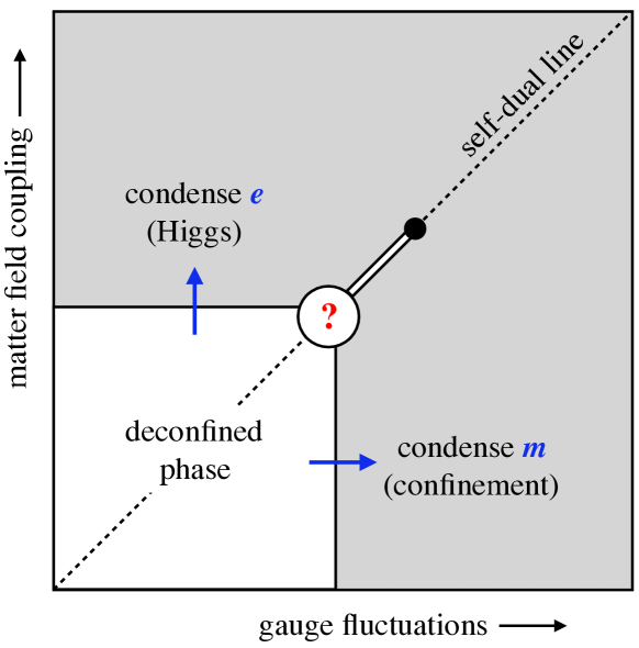
Figure 1: Topology of the phase diagram of $\mathbb{Z}_{2}$ gauge theory with matter. The shaded region is the trivial phase. The double line () represents a first-order line, ending at a standard critical endpoint (). The Higgs and confinement transitions have Ising exponents. The question mark shows the region studied in this paper. We give evidence for a scale-invariant, self-dual critical point.

In this paper we determine many of the properties of the self-dual transition using extensive Monte Carlo simulations and arguments based on the renormalization group and symmetry. Our numerical results include the first demonstration of scale-invariance at this transition, via scaling collapse of numerous observables. Our results for exponents also raise intriguing theoretical questions about how to understand this transition.

First, we give strong evidence that the transition is governed by a scale-invariant fixed point, for example via a striking scaling collapse that does not require any fitting parameters. We classify the leading local operators $S(r)$ and $A(r)$ as even and odd under duality symmetry respectively, and estimate their scaling dimensions $x_{S}$ and $x_{A}$ using scaling collapses and two-point functions. We check that three point functions are compatible with conformal invariance.

We also address some fundamental aspects of the anyon condensation transitions away from the self-dual line. As noted above, a key feature of the Higgs and confinement transitions is the possibility of using a Landau theory for a “fictitious” Ising order parameter. (These are sometimes referred to as “Ising^∗” transitions Nandkishore et al. (2012).) The emergence of this order parameter may be related to the question of where in the phase diagram certain “one-form” symmetries Kapustin and Thorngren (2017); Gaiotto et al. (2015); Wen (2019) emerge under coarse-graining. We propose an explicit construction of the fictitious Ising field (and of the string operators of the one-form symmetry). This construction is based on “repairing” or “patching” the membranes that appear in a geometrical representation of the partition function. We relate the feasibility of this patching operation to the question of whether $e$ and $m$ worldlines “percolate” in spacetime, and obtain the phase diagram for this percolation Huse and Leibler (1991) numerically. This shows that the fictitious Ising fields can be constructed on the Ising^∗ transition lines, but not at the self-dual critical point. However, we find that scale invariance at the self-dual transition can be diagnosed via the percolation of worldlines, and compute their universal fractal dimension $d_{f}$. (The result hints at a possible relation between exponents.)

We discuss the role of self-duality symmetry, arguing that it becomes an emergent internal symmetry in the IR. While our numerical analysis here is for the standard gauge-Higgs model, we also propose a modified lattice model, with a simpler action of duality, which it would be interesting to study further.

The dynamics of the Monte-Carlo algorithm (in Monte-Carlo time) correspond to a physically sensible universality class for the stochastic dynamics of membranes in 3D. We find that the dynamical exponent for this universality class is $z\simeq 2.48$ (not to be confused with the dynamical exponent $z_{\text{QM}}=1$ of the zero-temperature quantum dynamics in the 2+1D interpretation) and show that two-time correlation functions are another way to obtain $x_{A,S}$. The fact that the dynamical exponent is large is one of the challenges in simulating this model: unlike in many simple ordering transitions Newman et al. , no efficient nonlocal Monte Carlo update, that reduces $z$ to a small value, is known for this problem.

Various features of the fixed point make standard approaches to determining the precise location of the phase transition point, and the order of the transition, ineffective. These features include the structure of Binder cumulants close to the transition, the lack of any local operator with a small scaling dimension, and the fact that $x_{S}$ is very close to 1.5. (This is the threshold separating divergence and convergence of the heat capacity, and the proximity to this threshold leads to large scaling corrections in this quantity.) These features were the bane of our initial attempts at data analysis. We describe how they may be overcome, for example by focusing on appropriate dimensionless observables that allow a parameter-free scaling collapse.

Our numerical estimates for the exponents $x_{S}$ and $x_{A}$ turn out to be close to certain exponents in the XY universality class. This is remarkable in view of the mutual statistics of the condensing quasiparticles Vidal et al. (2009); Tupitsyn et al. (2010); Geraedts and Motrunich (2012a); Burnell (2018), which would make any relationship with the XY fixed point very surprising (Sec. X.4). The fixed point studied here is certainly distinct from the XY fixed point, as implied for example by the very different universal properties of the adjacent phases. On the other hand, it is not hard to find examples of pairs of 3D fixed points with exponents that are fairly close, but distinct. This issue requires further investigation. There are also many variations of the present model that remain to be studied (Secs. X.2, X.3, XI).

Textbook discussions of critical phenomena sometimes give the impression that studying universality in phase transitions is synonymous with studying Lagrangian quantum field theory. Therefore it is important to remember that there are critical points for which we so far lack any useful continuum Lagrangian (Sec. XI). Given that the self-dual transition is second-order, as previously suspected Tupitsyn et al. (2010); Vidal et al. (2009) and as the numerical evidence presented here shows, then it is perhaps the simplest example of one of these untamed beasts.

However, a rich variety of other topological transitions, with distinct (nontrivially braiding) anyons simultaneously becoming massless, are possible, with other discrete gauge theories providing further simple examples. Models with $\mathrm{U}(1)$ symmmetry are also interesting Geraedts and Motrunich (2012a, b); Lee et al. (2016); Geraedts and Motrunich (2012c, a), though they are more closely connected to continuum $\mathrm{U}(1)$ gauge theory (perhaps with Chern-Simons terms). A systematic program to understand all of these transitions would be valuable. Past results on the formulation of field theories for deconfined phase transitions Senthil et al. (2004); Levin and Senthil (2004); Motrunich and Vishwanath (2004); Senthil et al. (2005); Tanaka and Hu (2005); Senthil and Fisher (2006); Sandvik (2007); Bhattacharjee (2011); Wang et al. (2017); Gazit et al. (2018); Jiang and Motrunich (2019), where mutually nonlocal fields and Berry phases connecting different gapless degrees of freedom also play a key role, may provide some tools.

The $\mathbb{Z}_{2}$ deconfined phase is adjacent to another family of critical “quantum loop models” Freedman et al. (2004, 2005, 2008); Troyer et al. (2008); Dai and Nahum (2020) with no known Lagrangian description Dai and Nahum (2020). Interestingly, while these critical points may again be viewed in terms of membranes in spacetime, the obstacle to a continuum description is different there: a topological constraint on the dynamics, rather than the existence of massless particles with nontrivial braiding.

These different kinds of examples suggest that statistical ensembles of membranes Nelson et al. (2004) in three and four dimensions (elementary “string field theories” Polchinski (1998)) still hold many lessons for critical phenomena.

Contents

1. I Introduction
2. II The Ising gauge model
   1. II.1 As a lattice gauge theory
   2. II.2 As a model of membranes
   3. II.3 Manifestly self-dual loop representation
   4. II.4 Anyons and the toric code in a field
   5. II.5 Ising^∗ and first-order lines
3. III Self-duality as a symmetry
   1. III.1 Defining (anti)symmetric operators
   2. III.2 Spontaneous breaking of duality symmetry
4. IV Scale invariance
   1. IV.1 Initial obstacles
   2. IV.2 Parameter-free scaling collapse; RG trajectories
5. V Critical exponents
   1. V.1 Scaling collapse for $A$
   2. V.2 Scaling collapse for $S$
   3. V.3 Summary of exponents from the fits
6. VI Two-point correlators
7. VII Three-point function and conformal invariance
8. VIII Stochastic dynamics of membranes
   1. VIII.1 Universal dynamics and duality
   2. VIII.2 Dynamical scaling collapse
   3. VIII.3 Monte-Carlo updates
9. IX Membrane patching, emergent one-form symmetry, and worldline percolation
   1. IX.1 Patching membranes
   2. IX.2 Percolation summary
   3. IX.3 Percolation observables
10. X Related models
    1. X.1 An unusual self-dual loop model
    2. X.2 Perturbations of the gauge-Higgs model
    3. X.3 Dimensional crossovers
    4. X.4 Comparison with XY exponents
11. XI Outlook
12. A Membrane representation of $Z$
    1. A.1 Membranes on the original lattice
    2. A.2 Membranes on the dual lattice
    3. A.3 Manifestly self-dual representation
13. B First-order coexistence
14. C Details of MC scheme and of fits
15. D Further percolation data
    1. D.1 Percolation at the Ising^∗ transition ($x=1$)
    2. D.2 Percolation on the $y=1$ boundary
    3. D.3 Percolation on the self-dual line

II The Ising gauge model

The gauge-Higgs model has many guises. We begin by reviewing several equivalent formulations of the partition function we study and the basic features of the phase diagram. Readers should skip topics with which they are familiar.

II.1 As a lattice gauge theory

This is the standard formulation of $\mathbb{Z}_{2}$ gauge theory, with matter, on a cubic lattice Wegner (1971); Kogut (1979). ($\mathbb{Z}_{2}$ gauge theory is also referred to as “Ising” gauge theory.) The degrees of freedom are classical Ising matter fields ${\tau_{i}=\pm 1}$ on the sites $i$ of the lattice and gauge fields ${\sigma_{ij}=\pm 1}$ on the links $\left\langle ij\right\rangle$. The action includes a stiffness $K$ for the gauge fluctuations, and a coupling $J$ for the matter field. If $\square$ denotes a square plaquette, the partition function is:

$$Z\propto\sum_{\{\sigma\},\{\tau\}}\exp\left(K\sum_{\square}\left(\prod_{\left\langle ij\right\rangle\in\square}\sigma_{ij}\right)+J\sum_{\left\langle ij\right\rangle}\tau_{i}\sigma_{ij}\,\tau_{j}\right).$$ (1)

We work throughout on an ${L\times L\times L}$ torus. The action is invariant under the $\mathbb{Z}_{2}$ gauge transformation ${\tau_{i}\rightarrow\tau_{i}\chi_{i}}$, ${\sigma_{ij}\rightarrow\chi_{i}\sigma_{ij}\chi_{j}}$ with ${\chi_{i}=\pm 1}$. If desired, we can choose the gauge ${\tau_{i}=1}$, leaving a lattice model for the $\sigma$ spins on the links only, with terms $J\sigma$ on the links: this emphasizes that Eq. 1 is a lattice model with no internal global symmetries Wegner (1971). However along a line in the phase diagram it has a self-duality symmetry, as discussed below. In parts of the phase diagram the model also has one-form symmetries, either microscopic or emergent, which we discuss in Sec. IX.

It will be convenient to define Wegner (1971); Balian et al. (1974)

$$x =\tanh K, y =\tanh J.$$ (2)

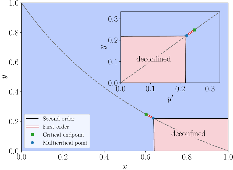
The phase diagram in this parameterization is shown in the main panel of Fig. 2. The dashed line is where the model is self-dual. The approximately rectangular region in the bottom right corner, at large gauge stiffness $K$ and small matter field coupling $J$, is the deconfined phase supporting deconfined anyons (Sec. II.4).

Figure 2: Sketch of phase diagram in the plane $(x,y)$. The gauge stiffness $K=\tanh^{-1}x$ increases to the right, and the matter field coupling $J=\tanh^{-1}y$ increases upwards (self-dual line shown dashed). Inset: same phase diagram in the $(y,y^{\prime})$ coordinates, where duality acts as a reflection. (The exponents below imply that the $e$ and $m$ condensation lines are asymptotically parallel as they approach the self-dual critical point, though the curvature is not visible at this scale.)

II.2 As a model of membranes

The model can be mapped to a statistical ensemble of “membranes” on the cubic lattice Huse and Leibler (1991); Gregor et al. (2011). In this picture, the parameters $x$ and $y$ control the microscopic surface tension for the membrane, and the microscopic line tension for membrane boundary respectively. The partition function is (see App. A for details):

$$Z(x,y)=\sum_{\mathcal{M}}\,x^{|\mathcal{M}|}\,y^{|\partial\mathcal{M}|}.$$ (3)

Here a membrane configuration $\mathcal{M}$ is simply any set of plaquettes of the cubic lattice: we call the plaquettes in $\mathcal{M}$ “occupied”. The energy of a configuration depends on the total number $|\mathcal{M}|$ of occupied plaquettes in the configuration, and on the total length of membrane “boundary”, ${|\partial\mathcal{M}|}$. This is the number of links where an odd number of occupied plaquettes meet. We refer to these as occupied links.

Note that the deconfined phase occurs in the regime where membrane surface is cheap, but membrane boundary is expensive. The extreme limit of the deconfined phase is $x=1$, $y=0$, where we have an ensemble of closed membranes with vanishing surface tension. We may exit the deconfined phase either by suppressing membrane area (decreasing $x$ sufficiently) or by tearing holes in the membranes (increasing $y$ sufficiently) Huse and Leibler (1991).

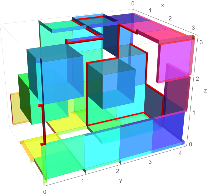
Fig. 3 shows a part of a membrane configuration taken from a simulation close to the self-dual critical point that we study. Plaquettes in $\mathcal{M}$ have been coloured (arbitrarily) and the boundary links in ${\partial\mathcal{M}}$ have been marked in red. The membrane representation suggests investigating “geometrical” (percolation-like) observables close to the critical point, as well as thermodynamic ones Huse and Leibler (1991). We discuss this in Sec. IX, showing that the loops in $\partial\mathcal{M}$ form a scale-invariant ensemble at the self-dual critical point.

The membrane picture is one way to see the duality property of the model Wegner (1971). In Eq. 3 the partition function is expressed as a sum over membrane configurations on the original cubic lattice. An alternative graphical representation yields an ensemble of precisely the same form, but for membranes on the dual cubic lattice (App. A), with dual values of the plaquette and link fugacities:

$$x^{\prime} \equiv\frac{1-y}{1+y}, y^{\prime} \equiv\frac{1-x}{1+x}.$$ (4)

This pair of mappings shows that $Z(x,y)$ is equal, up to a trivial constant, to $Z(x^{\prime},y^{\prime})$. Below we will see that duality can also be thought of as a conventional symmetry operation. This symmetry is not manifest in the formulations above, but may be made apparent in an alternate representation of the partition sum in terms of worldlines of $e$ and $m$ particles (Sec. II.3).

Note that, in view of Eq. 4, we are free to choose $(y,y^{\prime})$ as coordinates for the phase diagram, as in the inset to Fig. 2. The line $y=y^{\prime}$ is then the self-dual line, where the Boltzmann weights are invariant under duality symmetry.

Figure 3: Membranes with boundary: part of a configuration, close to the critical point on the self-dual line. Occupied plaquettes are shown coloured (colours have no meaning). Occupied links, where an odd number of plaquettes meet, are shown in red, thick.

II.3 Manifestly self-dual loop representation

The quantum interpretation reviewed in the next subsection motivates yet another representation of the path integral, in terms of two species of “loops”, which represent worldlines of both $e$ and $m$ particles. This representation makes self-duality manifest. The price we pay is minus signs in the Boltzmann weight, which encode the mutual semion statistics of the anyons $e$ and $m$.

The partition function can be written as (see App. A.3 for details):

$$Z\propto 4\sum_{\mathcal{C}_{e},\,\mathcal{C}_{m}}(-1)^{X(\mathcal{C}_{e},\mathcal{C}_{m})}y^{|\mathcal{C}_{e}|}{y^{\prime}}^{|\mathcal{C}_{m}|}.$$ (5)

The electric and magnetic worldline configurations ${\mathcal{C}_{e}}$ and ${\mathcal{C}_{m}}$, which we refer to as loop configurations, are sets of “occupied” links on the original and dual lattices respectively. See Fig. 4. Any even number of occupied links may be adjacent to each site, so the term “loops” is used loosely (see the footnote for details). $\mathcal{C}_{e}$ may be identified with the membrane boundaries $\partial\mathcal{M}$ in the previous representation.

Figure 4: Cubes of the original and dual lattices, with $e$ worldlines (red) and $m$ worldlines (blue) on the former and the latter respectively. (This configuration has linking number $X=1$.)

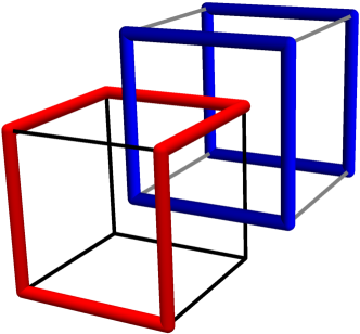
The crucial feature in Eq. 5 is the topological factor ${(-1)^{X}}$, which gives a factor of ${-1}$ for each linking between an $e$ worldline and an $m$ worldline. (That is, ${X(\mathcal{C}_{e},\mathcal{C}_{m})=0,1}$ is the $\mathbb{Z}_{2}$ linking number of the two worldline configurations. It can be computed, for example, by introducing an arbitrary membrane configuration $\widetilde{\mathcal{M}}$ such that ${\partial\widetilde{\mathcal{M}}=\mathcal{C}_{e}}$, and counting the number of intesections between $\widetilde{\mathcal{M}}$ and $\mathcal{C}_{m}$ modulo 2.) The values of the dual link fugacities $y$ and $y^{\prime}$ are defined in Eq. 2.

An interesting model of $\mathrm{U}(1)$ (oriented) flux lines with a linking sign has been studied in Geraedts and Motrunich (2012a) (see also variations in Refs. Geraedts and Motrunich (2012b); Lee et al. (2016); Geraedts and Motrunich (2012c, a)). That model has many features in common with Eq. 5, and also describes a problem of condensation of anyons with mutual statistics. However it also has significant differences as a result of a global $\mathrm{U}(1)\times\mathrm{U}(1)$ symmetry. We expect the $\mathrm{U}(1)\times\mathrm{U}(1)$ model to be described, at least in principle, by a continuum Chern-Simons gauge theory. The “$\mathbb{Z}_{2}\times\mathbb{Z}_{2}$” loop model in Eq. 5 is also closely related to a quantum wavefunction in 3+1D that sustains 2+1D $\mathbb{Z}_{2}$ topological order on its boundary Wang et al. (2015); Geraedts and Motrunich ; Von Keyserlingk et al. (2013).

Returning to Eq. 5, it is possible to sum over $\mathcal{C}_{m}$ exactly (App. A.3). We then return to the membrane expression (3) for the partition function, with $\mathcal{C}_{e}=\partial\mathcal{M}$. Similarly, integrating out $\mathcal{C}_{e}$ gives the dual membrane picture on the dual lattice. (Note that the line tension $y^{\prime}$ or $y$ of the species that is integrated out determines the surface tension of the membranes.)

However the representation (5) makes the duality symmetry that exists when $y=y^{\prime}$ (i.e. when $x=x^{\prime}$) manifest. We can think of the symmetry operation as a translation by ${(1/2,1/2,1/2)}$, where the lattice spacing of each cubic lattice is unity. This translation exchanges the cubic lattice with its dual, so exchanges $e$ and $m$ worldlines. Microscopically, this is not an internal symmetry (since it involves translation) but we will argue in Sec. III that self-duality becomes an internal $\mathbb{Z}_{2}$ symmetry of the IR theory.

Sec. X.1 presents an alternative loop model in which the $e$ and $m$ loops share the same lattice.

II.4 Anyons and the toric code in a field

The 3D gauge theory is expected to capture the universal physics of a wide range of 2+1D quantum models with a $\mathbb{Z}_{2}$ spin liquid phase. An anisotropic limit of the 3D theory, where the $z$ direction becomes a continuous imaginary time coordinate, maps exactly to the partition function for such a Hamiltonian on the square lattice. See Refs. Kogut (1979); Fradkin (2013) for details of such mappings. Here we review the basic excitations of the deconfined phase, and how they relate to the geometrical pictures above, in qualitative terms.

It is convenient to start with the toric code Kitaev (2003), a particularly simple model lying in the deconfined phase. The degrees of freedom are spin-1/2s on the links of the square lattice. The Hamiltonian includes a plaquette term and a vertex term:

$$H=-V\bigg{(}\sum_{\square}XXXX+\sum_{+}ZZZZ\bigg{)}.$$ (6)

The first product is a shorthand for the Pauli-X operators on the four links making up a given plaquette, and the second for the four Pauli-Z operators on the links touching a given site. Here $V$ is a coupling constant, which we have chosen equal for the two terms to ensure self-duality symmetry. Noting that we can equally well view spins either as living at the midpoints of bonds on the original square lattice or at the midpoints of bonds on the dual square lattice, the duality symmetry operation may be viewed as a translation by $(1/2,1/2)$, together with an exchange of $X$ and $Z$.

Figure 5: The relation between $e$ particles and membranes. Left: in the $Z$ basis, the toric code wavefunction is a superposition of strings of occupied links (bold) representing $Z=-1$, and an $e$ excitation is a vertex where an odd number of occupied links meet. Right: constructing a path integral (for a generic perturbed model) in this basis, worldsurfaces of strings become membranes $\mathcal{M}$ (grey), and worldlines of $e$ particles form the membrane boundary, or “loops”, ${\partial\mathcal{M}=\mathcal{C}_{e}}$. (The figure on the right is schematic: in the model we study, membrane configurations look like Fig. 3.)

Ground states have all the plaquette and vertex terms in Eq. 6 equal to 1, and are superpositions of “strings” — either on the original lattice (if we use the $Z$ basis, a link with $Z=-1$ being regarded as part of a loop) or the dual lattice (if we use the $X$ basis) Kitaev (2003). There are two fundamental types of excitation, related by duality. A vertex where $ZZZZ=-1$ is an “$e$ particle”, and a plaquette where $XXXX=-1$ is an “$m$ particle”. These are distinct types of anyon. Each is a boson, but adiabatically braiding an $e$ around an $m$ changes the sign of the wavefunction. (That is, they are mutual semions. The combination of an $e$ particle and an $m$ particle forms another type of anyon whose topological sector is denoted “$\epsilon$”: this also has $-1$ statistics with $e$ and $m$, but is a fermion Kitaev (2003); Nayak et al. (2008).) In the $Z$ basis, a $e$ excitation is the endpoint of a string (Fig. 5).

The toric code is a fine-tuned limit in which the $e$ and $m$ particles are non-dynamical. Critical phenomena are possible when the model is perturbed so that pair creation and annihilation of these particles becomes possible. This may be achieved by adding magnetic fields in both the $X$ and $Z$ directions Vidal et al. (2009); Tupitsyn et al. (2010). (For example, adding the operator $X$ to the Hamiltonian allows both hopping and pair creation/annihilation of bare $e$ particles on a given link.) The resulting model has been intensely studied Vidal et al. (2009); Dusuel et al. (2011); Tupitsyn et al. (2010); Wu et al. (2012). Duality exchanges these two magnetic fields, so that the line $h_{X}=h_{Z}$ preserves duality symmetry.

The phase diagram of the toric code in $X$ and $Z$ fields is expected to be equivalent to that discussed in the previous sections, up to nonuniversal constants Tupitsyn et al. (2010). The dimensionless field $h_{X}/V$, which can induce condensation of the $e$ particle, plays the role of the vertical coordinate in Fig. 1, and $h_{Z}/V$ plays the role of the horizontal coordinate.

The connection with the geometrical pictures above arises from writing the imaginary-time partition function in various choices of basis. We describe this only in qualitative terms:

In the $Z$ basis, the wavefunction is a superposition of terms like that illustrated in Fig. 5 (Left) with $e$ particles (at sites of the square lattice) forming endpoints of strings. Constructing the sum over Feynman trajectories using this basis, the worldsurfaces of strings form a set of membranes $\mathcal{M}$, and the worldlines of $e$ particles form a set of loops that are the boundaries ${\mathcal{C}_{e}=\partial\mathcal{M}}$ of these membranes. (In the limit $h_{X}=0$ there are no bare $e$ particles in the ground state, and correspondingly the membranes are closed surfaces.) This picture is a continuous-time version of that in Sec. II.2. The dual membrane picture is obtained by working in the $X$ basis, where the worldlines of $m$ particles are manifest.

Alternately we may pick a basis in which both the plaquette products $XXXX$ and the vertex products $ZZZZ$ are diagonal: this is possible since all these terms commute. The Feynman trajectory sum is then over worldline configurations $\mathcal{C}_{e}$ and $\mathcal{C}_{m}$ for both $e$ and $m$ particles, and is a continuous time version of the loop model in Eq. 5.

II.5 Ising^∗ and first-order lines

To conclude this overview of the model, we recap some features of the phase transition lines in Fig. 1 or equivalently Fig. 2.

Starting in the deconfined phase (in the lower-right hand corner of Fig. 2) we may exit it in three ways, two of which are related by duality Wegner (1971); Fradkin and Shenker (1979); Tupitsyn et al. (2010). Condensing the $e$ particle while keeping the mass of $m$ finite corresponds to the upper boundary of the deconfined region in Fig. 2 (main panel); this is the Higgs transition in the lattice gauge theory. Condensing $m$ while $e$ remains massive is equivalent by duality, and is the left-hand boundary of the deconfined region in Fig. 2 (main panel). This is the confinement transition in the lattice gauge theory.

These transitions are continuous with Ising exponents, at least sufficiently close to the boundaries of the phase diagram Kogut (1979), as we now rapidly review. These transitions, described by a weakly gauged Landau theory, are sometimes referred to as “Ising^∗” transitions (see for example Ref. Nandkishore et al. (2012)) to denote the fact that, because of gauging, only the $\mathbb{Z}_{2}$–even operators of the Ising CFT survive as local operators.

Consider first the Higgs transition in the limit $x=1$, i.e. infinite gauge stiffness $K=\infty$. The freezing of gauge fluctuations in this limit gives an exact mapping to a standard cubic lattice Ising model. But Ising exponents are retained at least along some part of the phase transition line, for finite $K$. This can be argued by fixing the gauge and deriving an effective longer-range Ising Hamiltonian perturbatively in $e^{-K}$ Wegner (1971); Fradkin and Shenker (1979). In the quantum language, the point is that so long as the $m$ and $\epsilon$ anyons are gapped, we can for many purposes neglect the fact that the $e$ particle which is condensing is an anyon, rather than a local excitation Burnell (2018). By duality, equivalent points hold for the confinement transition.

A more intuitive way to understand the relation to Ising is developed in Sec. IX and Ref. Nahum et al. . Let us start with the membrane representation in the limit where membrane boundary is completely suppressed ($y=0$ in Eq. 3, or $y^{\prime}=0$ in the dual membrane picture). Again this corresponds to the transitions on the boundaries of the phase diagram. In this limit the membranes form closed surfaces, so they may be mapped exactly to domain walls in a nearest-neighbor Ising model.

Now when we increase $y$ slightly, the membranes acquire holes in them. This means that there is no longer an unambiguous mapping to an Ising model. But if the holes are sufficiently small, we might expect this ambiguity to be unimportant on large scales, so that we can again think in terms of an ordering transition for a fictitious Ising order parameter.

We make this idea of a fictitious Ising order parameter precise using an explicit construction, based on the idea of “repairing” or “patching” the membranes in the representation (3) of the partition function (Sec. IX and Ref. Nahum et al. ). We argue that this construction can be performed all the way along the Ising^∗ critical lines, but not at the self-dual critical point, where a different universality class takes over.

For completeness, let us note that we can also think of the Ising^∗ transition in the loop model representation, Eq. 5. Loosely speaking, when one species of loops has a finite typical size, coarse-graining beyond this scale gives a loop model for a single species of unoriented loops. This is a standard representation of the Ising universality class, in terms of worldlines of the Ising quanta.

The self-dual transition point Fradkin and Shenker (1979); Jongeward et al. (1980); Tupitsyn et al. (2010); Vidal et al. (2009), where the two Ising^∗ lines meet, will be discussed in the rest of the text.

The line of first order transitions occurs within the trivial phase, so is relatively conventional. It is also a line where self-duality symmetry is spontaneously broken. The natural expectation is that the critical endpoint of this line is in the Ising universality class, with the Ising order parameter being the anti-self-dual operator defined below. Ising universality for this critical endpoint is consistent with a very rough estimate of the universal crossing value of the Binder cumulant, as shown in App. B.

In addition to these thermodynamic transitions we may also define geometrical transitions Huse and Leibler (1991) using the geometry of the membranes in Eq. 3 (Sec. D).

III Self-duality as a symmetry

We anticipate that, for any scale-invariant critical point on the self-dual line, self-duality becomes an internal $\mathbb{Z}_{2}$ symmetry of the IR theory.

One way to argue for this is via the manifestly self-dual representation of the partition function in Eq. 5 with $y=y^{\prime}$. This has a translation symmetry by $(1/2,1/2,1/2)$ which exchanges $e$ and $m$ worldlines. Correspondingly, the 2D quantum model in Sec. II.4 has a symmetry involving translation by ${(1/2,1/2)}$ that exchanges $e$ and $m$ particles.

The simplest assumption is that, at a scale-invariant critical point this microscopic symmetry gives rise to an internal $\mathbb{Z}_{2}$ symmetry of the IR fixed point theory. Loosely speaking, the action of the translation on the rescaled spatial coordinate of the coarse-grained theory disappears in the IR limit, so that the microscopic symmetry transformation should map to a purely internal symmetry transformation on the operators of the IR theory.

We can motivate this further by noting that alternative models for the deconfined phase can be constructed in which the duality symmetry, exchanging $e$ and $m$, is an internal symmetry even at the lattice level. Refs. Heinrich et al. (2016); Cheng et al. (2017) give exactly solvable 2D string-net Hamiltonians for the deconfined phase, with this property. We may also define a variant of the 3D loop model (5) in which the $e$ and $m$ loops live on the same lattice, with a $\mathbb{Z}_{2}$ symmetry exchanging them. This model is defined in Sec. X.1. It is plausible that by varying the interactions in either of these models we could access the same self-dual fixed point, at the corner of the deconfined phase, as in the original model.

The phase diagram of the gauge-Higgs model, restricted to the self-dual line, is shown schematically in Fig. 6. The first-order line in Fig. 1 corresponds to spontaneous breaking of self-duality symmetry, as discussed below.

Figure 6: The phase diagram on the self-dual line, i.e. on the line ${y=(1-x)/(1+x)}$ (where $x=x^{\prime}$ and $y=y^{\prime}$).

III.1 Defining (anti)symmetric operators

Duality acts on the phase diagram as $y\leftrightarrow y^{\prime}$. We would now like to define lattice operators $S$ and $A$ that are conjugate to the self-dual and anti-self-dual couplings, namely $y+y^{\prime}$ and $y-y^{\prime}$ respectively.

We continue to use the language of membranes (II.2). First, define “face” and “edge” operators, ${\mathcal{F}(p)}$ and ${\mathcal{E}(\ell)}$ respectively, which are equal to either zero or one and which measure whether a given plaquette $p$ or link $\ell$ of the cubic lattice is occupied in membrane configuration $\mathcal{M}$. That is, $\mathcal{F}(p)=1$ if $p\in\mathcal{M}$ and $\mathcal{F}(p)=0$ if $p\notin\mathcal{M}$; $\mathcal{E}(\ell)=1$ if $\ell\in\partial\mathcal{M}$ and $\mathcal{E}(\ell)=0$ if $\ell\notin\partial\mathcal{M}$.

The duality transformation maps these operators to operators on the dual lattice. By extending the transformation (App A) to the case of spatially varying couplings $x$ and $y$, we see that this mapping is

$$\mathcal{F} \longrightarrow-\frac{2x}{1-x^{2}}\,\mathcal{E}+\frac{x}{1+x},$$ (7)

$$\mathcal{E} \longrightarrow-\frac{2y}{1-y^{2}}\,\mathcal{F}+\frac{y}{1+y}.$$ (8)

We have suppressed plaquette/link indices to avoid clutter. The transformed operator on the RHS is located at the link/plaquette that is dual to the plaquette/link of the operator on the LHS.

Next let us symmetrize these operators with respect to the lattice point group. This naturally leads to operators that are centred either on a cube of the lattice, or on a vertex. We use $\mathcal{F}_{\text{cube}}(c)$ to denote the sum of $\mathcal{F}$ over the 6 plaquettes of a cube $c$, and $\mathcal{F}_{\text{vertex}}(v)$ to denote (one half times) the sum of $\mathcal{F}$ over the 12 plaquettes that touch a vertex $v$. Similarly $\mathcal{E}_{\text{cube}}(c)$ is (one half times) the sum over the 12 links in a cube and $\mathcal{E}_{\text{vertex}}(v)$ is the sum over the 6 links touching a vertex. (We include the factors of $1/2$ so that the expectation values of $\mathcal{E}_{\text{cube}}$ and $\mathcal{E}_{\text{vertex}}$ are equal, and similarly for $\mathcal{F}_{\text{cube}}$ and $\mathcal{F}_{\text{vertex}}$.)

Finally, specializing to the self-dual line, we define

$$A_{\text{cube}} =\mathcal{F}_{\text{cube}}+\frac{2x}{1-x^{2}}\mathcal{E}_{\text{cube}}-\frac{6x}{1+x}$$ (9)

$$S_{\text{cube}} =\mathcal{F}_{\text{cube}}-\frac{2x}{1-x^{2}}\mathcal{E}_{\text{cube}}+\frac{6x}{1+x}$$ (10)

and analogously for operators $A_{\text{vertex}}$ and $S_{\text{vertex}}$ at the vertices.

These operators transform simply under duality:

$$A_{\text{cube}} \longleftrightarrow-\,A_{\text{vertex}},$$ (11)

$$S_{\text{cube}} \longleftrightarrow+\,S_{\text{vertex}}.$$ (12)

In addition,

$$\sum_{c}A_{\text{cube}}(c) =\sum_{v}A_{\text{vertex}}(v),$$ (13)

$$\sum_{c}S_{\text{cube}}(c) =\sum_{v}S_{\text{vertex}}(v).$$ (14)

These “integrated” operators, which can be written either as sums over cubes or vertices, are the anti-self-dual and self-dual perturbations of the self-dual line.

Now we expand the lattice operators above in terms of continuum operators of a putative IR fixed point. Denote the leading $\mathbb{Z}_{2}$ odd and $\mathbb{Z}_{2}$ even scalar continuum operators by $A(r)$ and $S(r)$ respectively, with no subscript. We will also write $A_{\text{cube}}(r)$, $A_{\text{vertex}}(r)$, etc., for lattice operators, where $r$ is the location of the appropriate cube/vertex.

To be consistent with Eq. 11 and Eq. 14, the operator $S_{\text{cube}}$ must be of the form

$$S_{\text{cube}}(r)= (\text{self-dual operators})+$$

$$(\text{derivatives of anti-self-dual operators}),$$

and analogously for the other lattice $A$ and $S$ operators, so that their integrated versions have well-defined symmetry under duality. Taking into account point-group symmetry, some of the allowed terms in $S_{\text{cube}}$ and $S_{\text{vertex}}$ are:

$$S_{\text{cube}}(r) =\alpha S(r)+\beta\nabla^{2}A(r)+\gamma\nabla^{2}S(r)+\ldots$$ (15)

$$S_{\text{vertex}}(r) =\alpha S(r)-\beta\nabla^{2}A(r)+\gamma\nabla^{2}S(r)+\ldots.$$ (16)

Here $\alpha$, $\beta$ and $\gamma$ are nonuniversal constants. The sign of the $\mathbb{Z}_{2}$–odd term is reversed in the second line so that mixed correlators of lattice operators are consistent with Eq. 11. Equivalent formulae apply for the lattice $A$ operators, with $A$ and $S$ exchanged, and separate nonuniversal constants.

We will use the operators $A_{\text{cube}}$ and $S_{\text{cube}}$ in our simulations. We see that these lattice operators may be identified (up to derivative operators and other operators that are expected to be highly irrelevant) with the leading self-dual and anti-self-dual continuum operators.

From now on we will denote the lattice operators simply as $A(r)$ and $S(r)$, where $r$ is the coordinate of a cube. We will use $A$ or $S$, without an argument, to denote the spatially averaged quantity, for example

$$A=\frac{1}{L^{3}}\sum_{r}A(r).$$ (17)

We write $x_{A}$ and $x_{S}$ for the scaling dimensions of the two operators.

III.2 Spontaneous breaking of duality symmetry

Figure 7: Duality-breaking order parameter, $\sqrt{\langle A^{2}\rangle}$, as a function of $x$ on the self-dual line, for various system sizes (indicated in legend). Lines are just a guide to the eye. The deconfined phase is at larger $x$.

Figure 8: $\langle S\rangle$ as a function of $x$ for different system sizes. The legend indicates system size. The lines are just a guide to the eye.

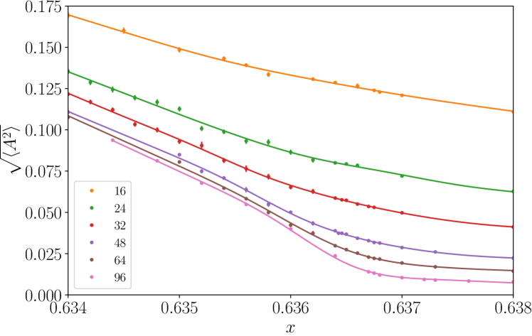
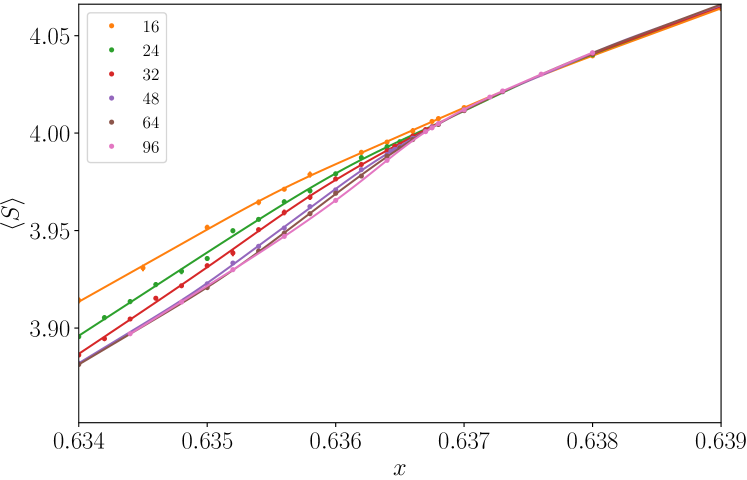
The phase diagram on the self-dual line was shown in Fig. 6. $A$ in Eq. 17 is an order parameter for the symmetry breaking that occurs when we exit the deconfined phase. By self-duality symmetry, its average vanishes,

$$\left\langle A\right\rangle=0,$$ (18)

but in the duality-broken phase its magnitude $\sqrt{\left\langle A^{2}\right\rangle}$ remains nonzero in the thermodynamic limit.

Raw data for this quantity are shown in Fig. 7, close to the critical point of interest. In all plots we parameterize the position along the self-dual line with $x$, so the deconfined phase corresponds to the right-hand-side of the figure. At first glance, Fig. 7 is consistent with the order parameter becoming nonzero in a continuous fashion below some $x_{c}$ (whose estimation we will discuss below).

The operator $S$, whose average is shown in Fig. 8, is analogous to the “energy” operator at a conventional classical transition, since it does not break symmetry: for a continuous transition, the correlation length exponent is

$$\nu=\frac{1}{3-x_{S}}.$$ (19)

The data in Figs. 7, 8 may be restated in terms of the average occupation of plaquettes and links in the membrane picture. On the section of the self-dual line where duality is spontaneously broken, there are two coexisting equilibria with different plaquette and link densities: we plot these two solutions explicitly in App. B. In the critical regime of interest here, the average occupation number of links is relatively small $\approx 2.5\%$, but despite this they make up a scale-invariant ensemble of loops (Sec. IX).

We now discuss how to establish the universal properties of the transition.

IV Scale invariance

IV.1 Initial obstacles

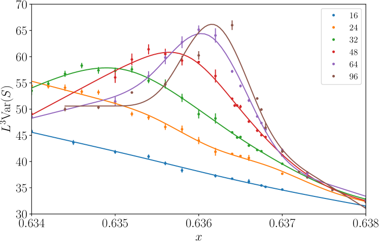
One standard means of locating a phase transition is to analyze the specific heat, which for many simple ordering transitions diverges at the critical point. If so, data for different system sizes can typically be scaled, allowing the critical point and correlation length exponent to be determined. Here the variable $S(r)$ is analogous to an energy, as discussed in the previous section, and ${L^{3}\operatorname{var}(S)}$ is analogous to a specific heat. Values for different system sizes are shown in Fig. 9.

At first sight the behaviour is the expected one: curves show a peak. But on closer inspection it is unclear whether the peak diverges at large $L$ or tends to a constant. It also becomes clear that variation of the width and height of the peaks does not follow the simple scaling form

$$\operatorname{Var}(S)=L^{-2x_{S}}f(z),$$ (20)

where $z=(x-x_{c})L^{1/\nu}$ and $\nu=1/(3-x_{S})$. At a first glance it looks like this transition will be plagued by large finite-size effects and it will be difficult to see any sign of scale invariance. In fact this is not the case; this will become clear after analyzing the behaviour of the variable $A$. (We will return to the specific heat below.)

Figure 9: The “heat capacity”: Variance of $S$ (multiplied by $L^{3}$) as a function of $x$ for different system sizes. The legend indicates system size. The lines are b-spline fits and are just a guide to the eye.

Another standard tool to determine the location of a critical point is the Binder cumulant for the order parameter Binder (1981). Here $A$ is our order parameter and we define a rescaled version of the Binder parameter:

$$\operatorname{b}_{4}(A)=-\frac{\kappa_{4}(A)}{2\kappa_{2}(A)^{2}},$$ (21)

where $\kappa_{n}(A)$ is the $n$-th order cumulant. With this normalization, $\operatorname{b}_{4}(A)$ becomes zero in the deconfined phase (where $A$ is disordered and has a Gaussian distribution) and tends to one in the first-order coexistence region (where $A$ has a two-delta distribution).

At a conventional second-order symmetry-breaking transition (e.g. Ising), the Binder parameter varies monotonically from zero to one, and different system sizes show a crossing that allows accurate location of the critical point. This is not the case here, as shown in Fig. 10. Rather than crossing, the curves present a minimum near $x=0.6367$. The curves do tend to touch here, consistent with scale invariance ($\operatorname{b}_{4}(A)$ is a dimensionless quantity, which should be asymptotically $L$-independent at a critical point), although some finite-size effects can be appreciated. A previous estimate of $x_{c}\approx 0.6359$ Tupitsyn et al. (2010) is not consistent with the location of the minimum (we will give a more accurate estimate below).

Figure 10: $\operatorname{b}_{4}(A)=-(1/2)\kappa_{4}(A)/{\rm Var}(A)^{2}$ as a function of $x$ for different system sizes. The legend indicates system size. The lines are b-spline fits and are just a guide to the eye.

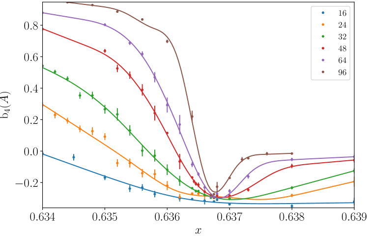
So, after a first look at these two standard quantities it is hard to assess whether the data obeys scaling collapse, and it seems at first sight that accurate estimation of $x_{c}$ will be more troublesome than for other systems and plagued by finite-size effects. Having reached this point, a key step for our understanding was analysing a parameter-free scaling collapse that we describe next.

IV.2 Parameter-free scaling collapse; RG trajectories

We advocate using a parameter-free procedure to determine the quality of scaling collapse of the data near a critical point. We construct a parametric plot using as coordinates two dimensionless quantities, $\operatorname{b}_{4}(A)$ and $\operatorname{b}_{1}(A)$ (defined below).

In the scaling region,

$$\operatorname{b}_{4}(A)=f(z),$$ (22)

where $z=(x-x_{c})L^{1/\nu}$. Other dimensionless ratios of cumulants are candidates for the second dimensionless quantity. Binder defined a ratio based on the sixth order cumulant: $V_{L}=\kappa_{6}(A)/(30\kappa_{2}(A)^{3})$ Binder (1981). High order cumulants are sensitive to the tails of the distribution and can be difficult to estimate accurately. Therefore we instead advocate using the ratio $\left\langle|A|\right\rangle/\left\langle A^{2}\right\rangle^{1/2}$:

$$\operatorname{b}_{1}(A)=\frac{1}{1-\sqrt{2/\pi}}\left(\frac{\left\langle|A|\right\rangle}{\kappa_{2}(A)^{1/2}}-\sqrt{\frac{2}{\pi}}\,\right).$$ (23)

The coefficients have again been chosen so that $\operatorname{b}_{1}(A)$ tends to zero in the deconfined phase and to one in the coexistence region. $\operatorname{b}_{1}(A)$ behaves qualitatively like $\operatorname{b}_{4}(A)$ in Fig. 10, and its expected scaling form is as in Eq. 22, with a different scaling function. For a standard Ising transition $\operatorname{b}_{1}$ goes monotonically from 0 to 1 with a crossing for different system sizes: there, it can be used to determine the critical temperature with the advantage of being slightly easier to estimate than $\operatorname{b}_{4}(A)$.

By plotting $\operatorname{b}_{4}(A)$ versus $\operatorname{b}_{1}(A)$ we obtain a parametric plot where $z$ is the parameter, see Fig. 11. If scaling is obeyed, points with different $x$ and $L$, but the same $z$, must overlap. This is a fair test of scale invariance because we do not have to fix or fit any parameters by hand and instead just plot raw data.

The data traces a trajectory from the point (0,0) to the point (1,1), showing very good overlap, except near the region $(\operatorname{b}_{1}(A),\operatorname{b}_{4}(A))\approx(-0.109,-0.285)$ where we see some finite-size effects. However, these finite-size effects become small for $L>32$. This figure represents on its own strong evidence that the multi-critical point is a second-order phase transition.

This figure can be also used to estimate the critical point. We construct “RG trajectories” in the ${(\operatorname{b}_{1}(A),\operatorname{b}_{4}(A))}$ plane by following the points for a fixed value of $x$ as $L$ is increased. The points representing a system (for a fixed generic $x$) should flow along the universal line towards either the (0,0) or the (1,1) fixed point. The inset of Fig. 11 shows this flow for two different $x$ values. For the system sizes used this simple procedure already determines the critical point with four digits of precision. We observe that for $x>0.6367$ the system flows towards (0,0), while for $x<0.6366$ it flows to (1,1). The repulsive fixed point is located (within the precision of the procedure) at the lower left extreme of the universal curve.

Figure 11: Parameter-free scaling collapse for $\operatorname{b}_{4}(A)$ as a function of $\operatorname{b}_{1}(A)$ for several system sizes (colored). Black stars mark the two phases: the deconfined phase at $(0,0)$ and the broken-duality phase (i.e. first-order coexistence) at $(1,1)$. Inset shows a zoom of the left lower corner of the main panel. Two selected $x$ values ($0.6364$ and $0.6370$) are highlighted and arrows are drawn in-between consecutive system sizes. Close to the critical point, $x\approx 0.6367$, values remain in a small region around $(\operatorname{b}_{1}(A),\operatorname{b}_{4}(A))\approx(-0.109,-0.285)$.

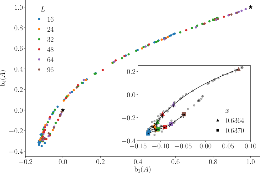
We see that the data in Fig. 10 should approximately scale for $L\gtrsim 32$ (fits are given below). A similar figure using ratios involving $S$ (e.g. $\operatorname{b}_{4}(S)$ or $\kappa_{3}(S)/\kappa_{2}(S)^{3/2}$) does not show good overlap, as expected from the discussion of Fig. 9. It would be strange to have very large finite-size effects in quantities depending on $S$ but not on those depending on $A$. The explanation turns out to be very simple. The exponent $x_{S}$ is very near 1.5, where the regular contribution to $\operatorname{Var}(S)$ cannot be neglected. When this is taken into account quantities depending on $S$ also obey scaling (Sec. V.2).

V Critical exponents

We turn to scaling fits in order to determine $x_{c}$ and the scaling dimensions of $A$ and $S$ ($x_{A}$ and $x_{S}$ respectively). Details of how fits were constructed may be found in App. C. The results of the various fits are summarized in Table 1.

Variable	$x_{c}$	$x_{S}$	$x_{A}$	$\chi^{2}$	d.o.f.
$\operatorname{b}_{1}(A)$	0.636660(16)	1.446(56)		49.53	46
$\operatorname{b}_{4}(A)$	0.636670(14)	1.445(62)		65.8	46
$\sqrt{\left\langle A^{2}\right\rangle}$	0.636702(20)	1.502(43)	1.222(16)	44.9	40
$\left\langle|A|\right\rangle$	0.636702(22)	1.510(48)	1.221(16)	43.1	40
$Var(S)$	0.636661(14)	1.5(fixed)		88.6	81
$\kappa_{3}(S)$	0.636651(18)	1.506(9)		68.6	66

Table 1: Results of fits. Errors shown are purely statistical.

V.1 Scaling collapse for $A$

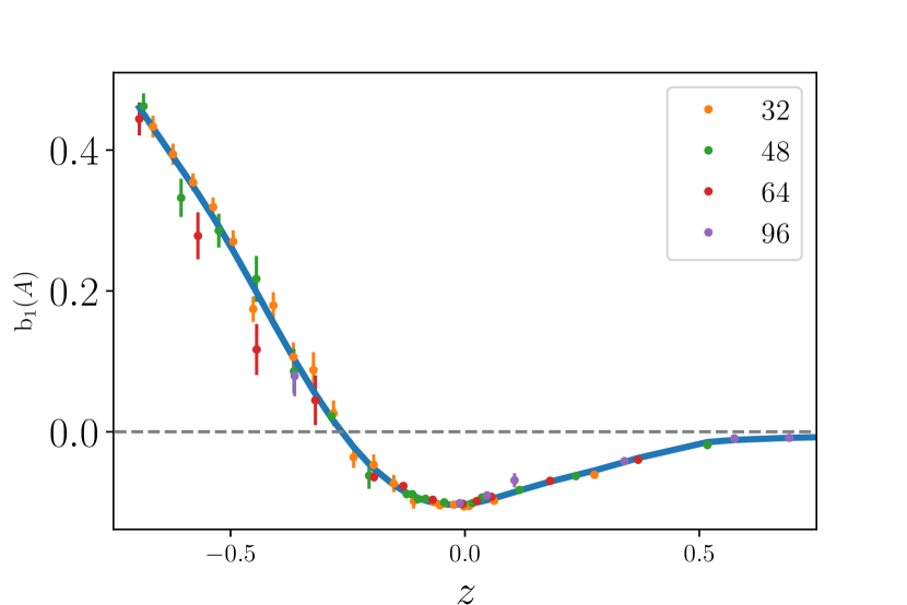
The scaling form for dimensionless quantities such as $\operatorname{b}_{1}(A)$ involves, in addition to the scaling function, the parameters $x_{c}$ and $\nu=1/(3-x_{S})$. Fig. 12 shows the scaling collapse of the data for $\operatorname{b}_{1}(A)$, and the fitted scaling function. The critical coupling $x_{c}$ obtained (Table 1) is very near the initial estimation made in section III.2 and $x_{S}$ is near 1.5, as noted above. A fit of $\operatorname{b}_{4}(A)$ gives very similar results (Table 1).

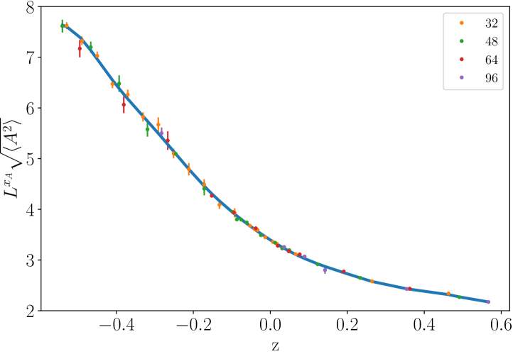
In order to obtain the exponent $x_{A}$ we fit

$$\sqrt{\left\langle A^{2}\right\rangle}=L^{-x_{A}}g(z).$$ (24)

The resulting scaling function, $g(z)$, is shown in Fig. 13 and the fitted parameters are indicated in Table 1. Fitting $\left\langle|A|\right\rangle$ yields similar results.

No finite-size-scaling corrections are included in these fits, although for ${L=32}$ these corrections are still non-negligible (compared to the error bars). If data for ${L=32}$ is excluded from the fits for $\operatorname{b}_{1}(A)$ and $\operatorname{b}_{4}(A)$ the estimates of $x_{S}$ increase.

Figure 12: Scaling collapse of $\operatorname{b}_{1}(A)$ versus scaling variable $z=(x-x_{c})L^{1/\nu}$, where $1/\nu=3-x_{S}$. The blue line corresponds to the fitted scaling function using B-splines with 12 degrees of freedom. The legend indicates the different system sizes.

Figure 13: Scaling collapse of $L^{x_{A}}\sqrt{\left\langle A^{2}\right\rangle}$ versus scaling variable $z=(x-x_{c})L^{1/\nu}$, where $1/\nu=3-x_{S}$. Blue line is the fitted scaling function using B-splines with 10 degrees of freedom. Legend indicates system sizes.

V.2 Scaling collapse for $S$

We have suggested above that the failure of a straightforward scaling collapse for $\operatorname{Var}(S)$ is due to $x_{S}$ being very close to $3/2$, the threshold where the regular contribution becomes comparable with the scaling contribution. Fortunately, a simple modification of the scaling ansatz should be accurate when ${|x_{S}-3/2|\ll 1/\log L}$:

$$L^{3}\operatorname{Var}(S)\simeq f(z)+4\pi\alpha_{S}^{2}\log(L).$$ (25)

Here $\alpha_{S}^{2}$ is the normalization constant for the two-point function of $S$ (Sec. VI). The function $f(z)$ includes a $z$-independent constant contribution, which arises from nonuniversal short-distance correlations.

Figure 14: Scaling collapse for $L^{3}(\operatorname{Var}(S)-C\log(L))$ versus scaling variable $z=(x-x_{c})L^{1/\nu}$, where $1/\nu=3-x_{S}$. The blue line corresponds to the fitted scaling function using B-splines with 10 degrees of freedom. Legend indicates different system sizes. In this fit only $x_{S}$ has been fixed to 3/2, see text for explanation of the scaling ansatz.

Figure 15: Scaling collapse for $L^{3x_{S}}\kappa_{3}(S)$ versus scaling variable $z=(x-x_{c})L^{1/\nu}$, where $1/\nu=3-x_{S}$. The blue line corresponds to the fitted scaling function using B-splines with 10 degrees of freedom.

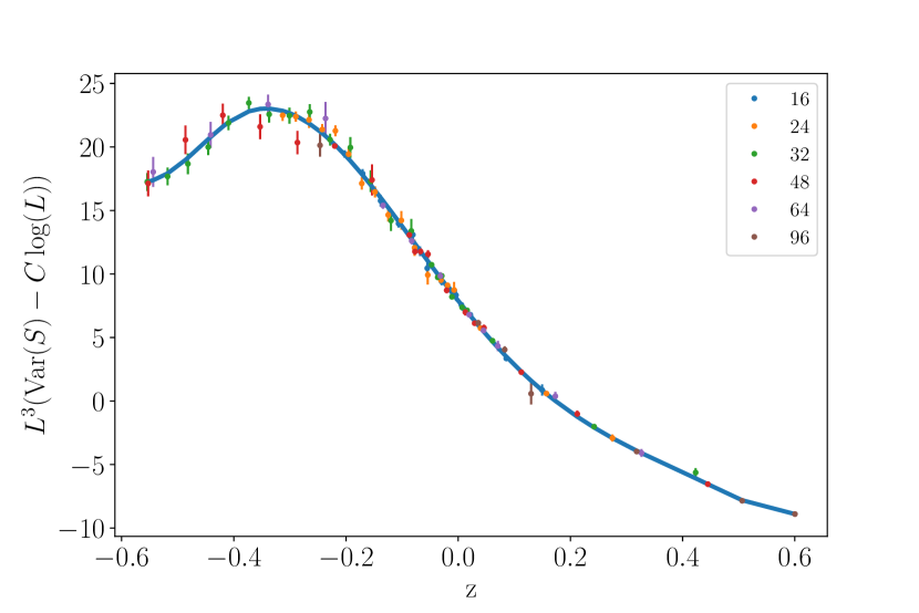
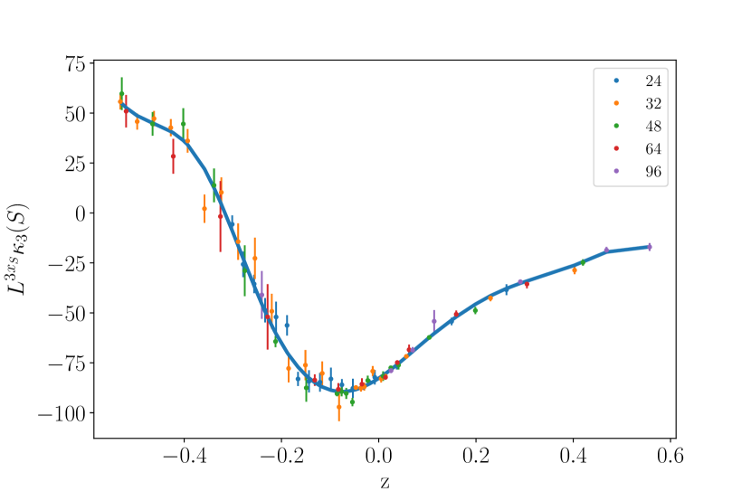
We have performed fits to this form keeping $\nu=2/3$ fixed (in line with the approximation above) so that only the critical coupling $x_{c}$ and the coefficient ${C=4\pi\alpha_{S}^{2}}$ of the logarithm can be adjusted to obtain scaling collapse. The scaling function is shown in Fig. 14. We obtain a good fit, even when data from small system sizes are included. The estimated $x_{c}$ is again very similar to previous estimates. Also, the constant $C=10.05(23)$ obtained is consistent with our calculation of the correlation function in the next section. In summary, the fit to $\operatorname{Var}(S)$ is consistent with the correlator of $S$ obeying scaling with $x_{S}$ very close to 3/2 (indeed, allowing $\nu$ to be free in this fit, instead of fixed to $2/3$, did not improve the fit quality).

An alternative way to avoid dealing with the regular contribution is to analyze higher-order cumulants. The singular contribution near a critical point scales as ${\kappa_{n}(S)=L^{-nx_{S}}f(z)}$, while the regular contribution should scale as $\kappa_{n}(S)_{\text{regular}}\propto L^{-d(n-1)}$. For $x_{S}\approx 3/2$ and $n=2$ both contributions scale in the same way, but for $n=3$ the singular contribution should dominate. Indeed the data for $\kappa_{3}(S)$ can be collapsed, as shown in Fig. 15. We obtain $x_{c}$ and $x_{S}$ values fully consistent with previous results (Tab. 1), although it is worth noting that the statistical error of $x_{S}$ is much smaller.

V.3 Summary of exponents from the fits

We have provided clear evidence that the Ising gauge-Higgs model has a scale-invariant multicritical point. Simulations are inevitably restricted to finite lengthscales, so can never rigorously exclude an extremely weak first-order transition; but all of the observables we have examined exhibit good scaling collapse, with fairly modest finite-size effects.

As there are some finite-size effects, we consider a reasonable confidence interval for the critical point to be $x_{c}\in[0.63665,0.6367]$. For the study of correlation functions in the next sections we round to four digits and consider critical behaviour at $x_{c}\approx 0.6367$.

For the exponent $x_{S}$, the value obtained from $\kappa_{3}(S)$ (Table 1) has the smallest statistical error and we take it as a reference in the following. Our statistical error bars do not take into account possible systematic errors related for example to finite size effects, so a realistic confidence interval should be larger; however, we have verified that dropping the smaller system sizes in the fit only very slightly increased $x_{S}$, remaining within the statistical error bars.

Our estimate of $x_{S}$ leads to $\nu=0.669(4)$. This is not too far from estimates $\nu\approx 0.7$ Vidal et al. (2009) and $\nu\approx 0.69$ Dusuel et al. (2011) based on the calculation of the gap in the toric code using small-field series expansions (up to eighth order). However, a basic issue with the series expansion method is that it cannot detect a first-order transition Vidal et al. (2009), i.e. it must assume a continuous transition rather than demonstrating one. Ref. Dusuel et al. (2011) attempts to rectify this by comparing estimates of the ground state energy from series expansion with a variational wavefunction, but we expect that the accuracy with which this method could detect a weak first order transition is severely limited by the accuracy of the variational wavefunction.

A realistic confidence interval for $x_{A}$ should again be larger than the statistical one in Tab. 1. We note that the $x_{c}$ estimates obtained from $\sqrt{\left\langle A^{2}\right\rangle}$ and $\left\langle|A|\right\rangle$ are slightly larger than for the other fits; if we estimate $x_{A}$ keeping $x_{c}=0.63666$ fixed, then the value drops to 1.20, slightly below the statistical confidence interval.

Standard scaling relations Cardy (1996) imply that the order parameter exponent $\beta$, defined by ${\sqrt{\left\langle A^{2}\right\rangle}\sim(x_{c}-x)^{\beta}}$ in the infinite system, is ${\beta=x_{A}/(3-x_{S})}$ (compare Fig. 7). Asymptotically close to the self-dual critical point, the shape of the Higgs and confinement lines in the inset to Fig. 2 should be ${y_{-}\sim\pm|\delta y_{+}|^{(3-x_{A})/(3-x_{S})}}$, where ${y_{\pm}=(y\pm y^{\prime})}$ gives the self dual and anti-self-dual couplings. Since ${(3-x_{A})/(3-x_{S})}$ is a little larger than one, the Higgs and confinement lines are asymptotically parallel as they approach the critical point.

The values obtained for the critical exponents clearly differ from Ising values, but they are surprisingly close to certain exponents in the XY model. This point will be discussed in Sec. X.

VI Two-point correlators

Figure 16: Two-point correlators for the operators $A$ (top) and $S$ (bottom). The displacement between the two operators is taken parallel to a lattice direction. Dashed lines are fits of the $L=64$ data in the range $r\in[10,15]$ to the forms in Eq. 27 with $x_{A}=1.224$, $x_{S}=1.506$ fixed and $\alpha_{A,S}$ free, giving $\alpha_{A}^{2}=0.72$ and $\alpha_{S}^{2}=0.77$.

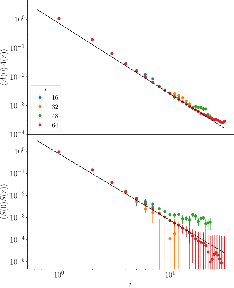
We now show that two-point functions of the local operators $A(r)$ and $S(r)$ are consistent with scale invariance,

$$\left\langle A(0)A(r)\right\rangle =\frac{\alpha_{A}^{2}}{r^{2x_{A}}}, \left\langle S(0)S(r)\right\rangle_{\text{conn}} =\frac{\alpha_{S}^{2}}{r^{2x_{S}}}.$$ (27)

Fig. 16 compares data for the critical two-point functions to such power-law fits, giving good agreement at larger separations. The exponents $x_{A}$ and $x_{S}$ in the fits have been fixed to the values $1.224$ and $1.506$, respectively (see Tab. 1), while the nonuniversal constants $\alpha_{A,S}$, which we will require in Sec. VII, have been left free.

The simulations also give access to dynamical correlation functions in Monte-Carlo time, which we analyze in Sec. VIII. These also encode the exponents $x_{A}$ and $x_{S}$, together with a dynamical exponent $z$.

VII Three-point function and conformal invariance

Figure 17: Test of conformal invariance: ratios of the three-point correlators defined in the text. Assuming exponent values $x_{A}=1.224$, $x_{S}=1.506$, conformal invariance requires these ratios to converge at large $r$ to the values indicated by dashed lines (error bars are from variation between 6 samples). We find agreement with the predicted value, within error bars, once $r\gtrsim 3$. Error bars become too large for a useful comparison once $r>4$.

Conformal invariance fixes the three point functions in terms of the fields’ scaling dimensions and operator product expansion (OPE) coefficients Cardy (1996). Conversely, data for three-point functions allow a direct numerical test of conformal invariance.

The OPE coefficients for the fields $A$ and $S$ that are allowed by duality symmetry to be nonzero are $C_{AAS}$ and $C_{SSS}$. Here we examine the three-point function $\left\langle A(0)A(\bm{\mathbf{r}})S(\bm{\mathbf{r}}^{\prime})\right\rangle_{\text{conn}}$ and give a very rough estimate of the corresponding OPE coefficient $C_{AAS}$. Data for $\left\langle S(0)S(\bm{\mathbf{r}})S(\bm{\mathbf{r}}^{\prime})\right\rangle_{\text{conn}}$ was too noisy for a similar analysis.

The form dictated by conformal invariance for the three-point function is

$$\left\langle A(0)A(\bm{\mathbf{r}})S(\bm{\mathbf{r}}^{\prime})\right\rangle_{\text{conn}}=\frac{C_{AAS}\times\alpha_{A}^{2}\alpha_{S}}{|\bm{\mathbf{r}}|^{2x_{A}-x_{S}}|\bm{\mathbf{r}}^{\prime}|^{x_{S}}|\bm{\mathbf{r}}-\bm{\mathbf{r}}^{\prime}|^{x_{S}}}.$$ (28)

where $\alpha_{A,S}$ are the same operator normalization constants that appear in the two-point functions (27).

We consider four possible spatial arrangements for the three points in the correlator, lying either on a line ($L$) or on the vertices of a right triangle ($D$):

$$L_{AAS}(r) \equiv\left\langle A(0,0,0)A(r,0,0)S(2r,0,0)\right\rangle_{\text{conn}},$$ (29)

$$L_{ASA}(r) \equiv\left\langle A(0,0,0)S(r,0,0)A(2r,0,0)\right\rangle_{\text{conn}},$$ (30)

$$D_{AAS}(r) \equiv\left\langle A(0,0,0)A(r,0,0)S(r,r,0)\right\rangle_{\text{conn}},$$ (31)

$$D_{ASA}(r) \equiv\left\langle A(0,0,0)S(r,0,0)A(r,r,0)\right\rangle_{\text{conn}}.$$ (32)

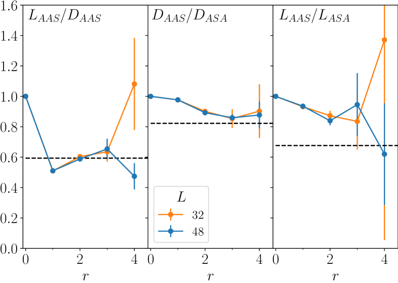
We use ratios of these three-point functions to test for conformal invariance. The CFT prediction depends only on $x_{A}$ and $x_{S}$ (and on the arrangement of points in the correlator), so this test does not require an independent estimate of the nonuniversal constants $\alpha_{A,S}$ in Eq. 28.

Fig. 17 compares each of the three independent 3-point function ratios with the CFT prediction (for $x_{A}=1.224$, $x_{S}=1.506$), which is marked with a dashed line. Modulo uncertainty in the exponent estimates, the data should converge to these lines at large $r$. Statistical errors limit us to small $r$, because of the rapid decay of the 3-point functions with $r$. Despite this, there is agreement, within errors, with the CFT prediction once $r\gtrsim 3$.

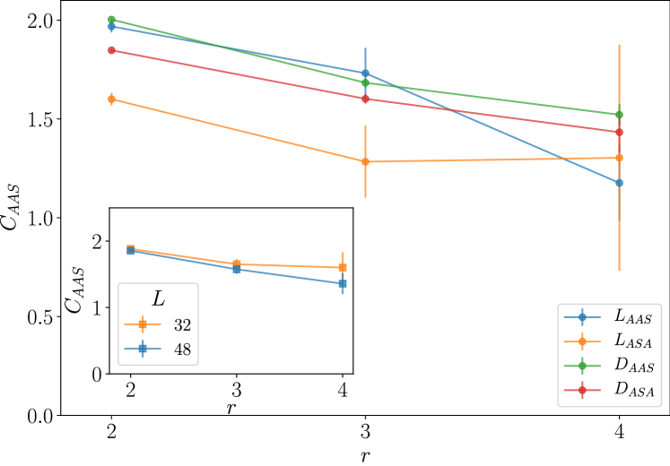
Motivated by this consistency, we make a very preliminary estimate of the universal constant $C_{AAS}$. Fig. 18 shows finite-$r$ estimates obtained from Eq. 28 (for each geometry of 3-point function). The data suggest that ${C_{AAS}\sim 1.5}$. The uncertainty is large, because of the very small range of $r$, and because the uncertainty in $\alpha_{A,S}$ (obtained from the 2-point function in Sec. VI) is hard to estimate. It would be worthwhile to improve this estimate. Refs. Caselle et al. (2015) and Hasenbusch (2020a) discuss methods for numerical estimation of OPE coefficents.

Figure 18: Main panel: Finite-$r$ estimates of the OPE coefficient $C_{AAS}$ using 3-point functions with four different geometries, using data from system size $L=48$ (error bars are from variation between 6 samples). Inset: Average of the four estimates for $L=48$ and also for $L=32$.

VIII Stochastic dynamics of membranes

So far we have discussed the gauge theory as a problem of equilibrium statistical mechanics in either 2+1 or 3+0 dimensions. But our simulations involve a fourth coordinate, which is Monte Carlo time (denoted $t$). The Monte Carlo dynamics may be interpreted physically as a model for stochastic thermal motion of classical membranes (Sec. II.2), or alternately of classical spins in 3D (Sec. II.1). These dynamics contain additional universal data beyond the data in static correlations: most importantly, the dynamical exponent $z$ that dictates how the typical relaxational timescale $\tau$ scales with system size $L$ at the critical point, ${\tau\sim L^{z}}$. Two-time correlation functions in this dynamics are also an alternative means of determining the exponents $x_{A}$ and $x_{S}$, as shown below.

VIII.1 Universal dynamics and duality

There is great freedom in the microscopic definition of the stochastic dynamics, i.e. the choice of update for our Monte Carlo Markov chain. But we expect to find a dynamical fixed point that embraces a large class of microscopic updates that are local and preserve detailed balance (our updates are local and are described in Sec. VIII.3 below). This is analogous to, say, the critical 3D Ising model which shows a robust universality class for spin-flip dynamics with no conservation laws (the universality class of “Model A” Glauber (1963); Hohenberg and Halperin (1977); Wansleben and Landau (1987, 1991); Münkel et al. (1993); Ito (1993); Grassberger (1995); Jaster et al. (1999); Ito et al. (2000); Murase and Ito (2007); Collura (2010); Niermann et al. (2015); Mesterhazy et al. (2015); Duclut and Delamotte (2017); Adzhemyan et al. (2018); Hasenbusch (2020b)).

As in the Ising model, the dynamical universality class may change if we introduce conservation laws Hohenberg and Halperin (1977). For example, dynamics that conserve the total membrane area (the total number of occupied plaquettes) could be relevant to some experimental settings. The dynamical universality class may also change if we include nonlocal updates in the Monte Carlo simulations: finding a nonlocal update that speeds up simulations by reducing $z$ is a challenging open problem (Sec. XI).

The present dynamical critical point has one subtlety that arises from self-duality. We have argued that self-duality is a $\mathbb{Z}_{2}$ symmetry of the 3D fixed point, allowing us to classify scaling operators as $\mathbb{Z}_{2}$ even or odd ($S$ and $A$ respectively). The mixed correlator $\left\langle AS\right\rangle$ therefore vanishes in the equilibrium ensemble. But the Monte-Carlo dynamics itself is not $\mathbb{Z}_{2}$-symmetric Jongeward et al. (1980). To define the dynamics we had to choose one of the two dual representations, either on the original cubic lattice or on its dual, breaking the symmetry between them. As a result, the mixed correlator $\left\langle AS\right\rangle$ can be nonzero for non-equal times.

Assuming that the scaling operators ${A(r)}$ and ${S(r)}$ of the three-dimensional theory are lifted to scaling operators ${A(r,t)}$ and ${S(r,t)}$ in the dynamical theory, standard dynamical scaling Hohenberg and Halperin (1977) at large $|r|$ and $t$ gives:

$$\left\langle A(r,t)A(0,0)\right\rangle =t^{-{2x_{A}}/{z}}F_{AA}(t/|r|^{z},t/L^{z}),$$ (33)

$$\left\langle S(r,t)S(0,0)\right\rangle =t^{-{2x_{S}}/{z}}F_{SS}(t/|r|^{z},t/L^{z}),$$ (34)

$$\left\langle A(r,t)S(0,0)\right\rangle =t^{-{(x_{A}+x_{S})}/{z}}F_{AS}(t/|r|^{z},t/L^{z}).$$ (35)

The $\mathbb{Z}_{2}$ symmetry of the equilibrium critical point ensures that the last line vanishes at equal time.

Figure 19: Main panels: Scaling collapse of autocorrelation functions for $\langle A(0)A(t)\rangle$ (top), $\langle S(0)S(t)\rangle$ (center) and $\langle S(0)A(t)\rangle$ (bottom) as a function of $t/L^{z}$ (using $x_{A}=1.224$ and $x_{S}=1.506$). Inset: Autocorrelation time as a function of system size for 4 different correlators: $\langle E(0)E(t)\rangle$ (blue triangle), $\langle A(0)A(t)\rangle$ (orange triangle), $\langle S(0)S(t)\rangle$ (green pentagon), $\langle S(0)A(t)\rangle$ (red star). Straight line fits all the data points to a power-law $\tau=AL^{z}$ with $z=2.48$.

VIII.2 Dynamical scaling collapse

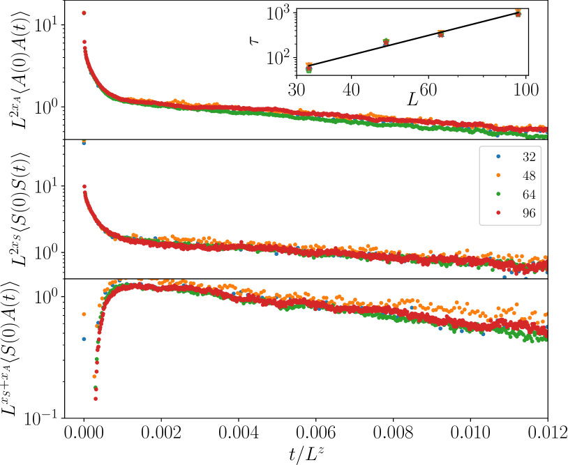
First we obtain the dynamical exponent from the typical relaxation timescale $\tau(L)$ of a sample of size $L$. We estimate this timescale from the exponential decay of various two-time correlators, in particular those of $S$ and $A$ (inset to Fig. 19). The various estimates are consistent with each other, and fitting $\tau(L)$ to a power law gives:

$$z\simeq 2.48.$$ (36)

For comparison, this is larger than the dynamical exponent for spin flip dynamics in the 3D Ising model Wansleben and Landau (1987, 1991); Münkel et al. (1993); Ito (1993); Grassberger (1995); Jaster et al. (1999); Ito et al. (2000); Murase and Ito (2007); Collura (2010); Niermann et al. (2015); Mesterhazy et al. (2015); Duclut and Delamotte (2017); Adzhemyan et al. (2018); Hasenbusch (2020b), for which a recent estimate is $z=2.0245(15)$ Hasenbusch (2020b).

The main panel of Fig. 19 demonstrates scaling collapse for the temporal correlators of the spatially averaged operators $A$ and $S$, using this exponent. (The relevant scaling forms are given by integrating Eqs. 33–35.) Results are consistent with expectations from Sec. VIII.1, including the continuous vanishing of the scaling function for $\left\langle S(0)A(t)\right\rangle$ as $t\rightarrow 0$.

VIII.3 Monte-Carlo updates

The simplest Monte Carlo update is one that flips the state of a single plaquette with the appropriate Metropolis probability. However, a notable feature of configurations close to the multi-critical point is that only a very small fraction ($\approx 2.5\%$) of links are occupied. When occupied links are rare, an attempted plaquette update has a high chance of creating four new occupied links, significantly increasing the energy, and therefore a high chance of being rejected.

This suggests that while plaquette updates are necessary for allowing occupied links to move, they are inefficient at moving surfaces around. To speed up the equilibration of surfaces we therefore combine plaquette updates with a second update that flips the state of all six surfaces of a cube. Since this move never changes the number of occupied links, it does not face the problem above. Since this move is still a local update we do not expect it to change $z$, as we have confirmed numerically. See App. C for further details including the scheme for parallelization.

IX Membrane patching, emergent one-form symmetry, and worldline percolation

In this section we widen our focus to transitions out of the deconfined phase generally. We give a construction for the “fictitious” Ising order parameters (that are the key feature of Ising^∗ transitions) on the Higgs and confinement lines. We find that these fictitious order parameters can be constructed all the way along the Ising^∗ lines, but not at the self-dual critical point. The disappearance of the fictitious order parameter at the self-dual critical point is associated with the emergence of a scale-invariant ensemble of loops there.

Studying this ensemble of loops with percolation-like observables Huse and Leibler (1991); Cardy (1996) allows another numerical test of scale-invariance at the self-dual critical point, and gives another critical exponent with which to characterize it (Secs. IX.2, IX.3).

IX.1 Patching membranes

The fact that the $e$ and $m$ condensation transitions have Ising exponents (away from the self-dual line) is easy to understand at the boundaries of the phase diagram (Fig. 2), as reviewed in Sec. II.5 Wegner (1971); Fradkin and Shenker (1979). In these limits the partition function can be written as a sum over closed membrane configurations. Mapping these closed membranes to Ising domain walls gives the relation to Ising.

Moving away from this extreme limit, the membranes acquire “holes” Huse and Leibler (1991). (We use the term “hole” loosely: more precisely, we mean any connected cluster of links in $\partial\mathcal{M}$, as defined in Sec. II.2.) But it is natural to think that, if these holes have a finite typical size, coarse-graining beyond this size may restore a picture in terms of closed membranes that can be interpreted as Ising domain walls. This is a heuristic explanation for why an effective Landau theory is useful even some distance away from the boundary of the phase diagram.

Here we wish, first, to give an explicit construction of these emergent degrees of freedom. Our approach is simply to “repair” the membranes $\mathcal{M}$ in a given configuration. We will be schematic, deferring further details and a numerical demonstration to Ref. Nahum et al. . Second, we wish to understand what happens to the fictitious order parameter when move along the Ising^∗ transition line towards the self-dual critical point. This issue is closely connected to the question of where in the phase diagram emergent “one-form” symmetries Kapustin and Thorngren (2017); Gaiotto et al. (2015); Wen (2019) exist.

We consider the membrane ensemble in Eq. 3, which is convenient for describing one of the two dual one-form symmetries. By duality, analogous considerations apply for the dual symmetry. (The Ising^∗ transition that we discuss below is the $m$ condensation line.)

Let us briefly make the connection with a formal point of view. The fictitious Ising order parameter will make sense if (perhaps after coarse-graining) we can consistently define string operators $V_{P}=\pm 1$, supported on arbitrary paths $P$ in spacetime, that count the parity of the number of membranes that intersect $P$. Let us assume that we can define such operators which are functions of the membrane configuration $\mathcal{M}$, and whose value is unchanged if the shape of the path $P$ is deformed (while preserving the locations of the endpoints, if $P$ is not a closed loop). We can then define a coarse-grained Ising variable $\phi_{r}$, up to a global $\mathbb{Z}_{2}$ ambiguity, by identifying $\phi_{r}\phi_{r^{\prime}}$ with $V_{P}$ for any path $P$ between $r$ and $r^{\prime}$. (Here for simplicity we consider an infinite system.)

Such string operators, obeying an invariance under deformations, define a $\mathbb{Z}_{2}$ one-form symmetry (see Ref. Gaiotto et al. (2015); Wen (2019) for definitions). Switching briefly to the language of 2D quantum states, the analogous quantum operators in the toric code are simply the familiar topological string operators Kitaev (2003) which can be used to create pairs of $m$ anyons at their endpoints (a similar dual operator creates pairs of $e$ anyons). Perturbing away from the solvable limit of the toric code, dressed versions of these string operators are expected to exist in principle so long as the other anyons, which braid nontrivially with $m$, remain gapped Hastings and Wen (2005); Wen (2019).

Figure 20: Membrane patching process (schematic). A configuration $\mathcal{M}$ of membranes, with a non-empty boundary $\partial M$ made up of finite clusters of occupied links (shown red) is “patched” by attaching finite surfaces (blue) to the components of $\partial\mathcal{M}$. In the resulting ensemble of closed membranes, line operators may be defined, specifying an emergent one-form symmetry. A “fictitious” scalar field ${\phi=\pm 1}$ may also be introduced, whose domain walls are the patched membranes. The Ising^∗ transition is the ordering transition for this fictitious field.

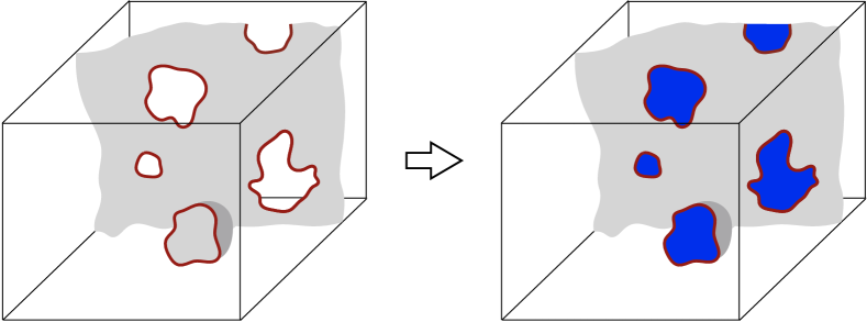
Returning to the membrane picture, how would we explicitly define such string operators, or the $\phi_{r}$ configuration, in a simulation? A natural approach is to start with the membrane configuration, and try to “patch up” the holes, to give closed membranes. This is not a strictly local process, since holes can be of any size. We also have some freedom in the convention, or algorithm, for constructing the patching surfaces. But, if holes have a finite typical size, and large holes are exponentially rare, we expect the nonlocality in the patching operation to be mild. Each finite “loop” (cluster of links) in $\partial\mathcal{M}$ may be patched by attaching a finite surface of comparable size. This is illustrated in Fig. 20.

Having done this, we may define $\phi_{r}$ (again with a global $\mathbb{Z}_{2}$ freedom). Because of the nonlocality of the patching operation, this effective field only really makes sense on lengthscales larger than the typical size of a loop. (It will therefore be most useful as an effective field in a Lagrangian when it has a correlation length that is parametrically larger than this loop size, or infinite.) This construction allows us in principle to compute the “two-point” correlation function of $\phi_{r}$ in a simulation, and extract the corresponding anomalous dimension, despite the fact that $\phi_{r}$ is not a local gauge invariant quantity Nahum et al. .

We may also define thickened string operators. Let $P$ be, say, a straight path of length $\ell\gg 1$. In order to determine how many domain walls $P$ passes through after patching, we must check how many loops $P$ threads in the unpatched configuration $\mathcal{M}$. This requires us to examine a cigar-shaped region around $P$, wide enough to contain (with probability close to one) all the loops which $P$ threads. The operator $V_{P}$ is therefore a function of the degrees of freedom within this cigar-shaped region. When large loops are exponentially suppressed, the largest loop that $P$ threads will typically be of size ${\sim\ln\ell}$ (due to rare large loops), so the typical width of the cigar should be of this order. However, close to the endpoints of $P$, it is sufficient for the width to be only somewhat larger than the typical loop size (i.e. $\ell$-independent).

The above pertains to the case where the “holes” have a finite typical size $\xi_{h}$. If on the other hand $\xi_{h}$ diverges, so that samples of arbitrarily large size $L$ contain holes of size comparable with $L$, then this procedure for defining the string operator and effective Ising order parameter is liable to fail (since $\phi_{r}$ and $V_{P}$ can become highly nonlocal). That is, a sufficient condition for this procedure to work is that the appropriate set of worldlines, $\partial\mathcal{M}$, is in the non-percolating phase when viewed as a bond percolation configuration.

For this reason it is interesting to revisit the question of where in the phase diagram these worldlines percolate Huse and Leibler (1991), which we do next. For example, as we move along the confinement transition line, starting at $y=0$ (where there are no worldlines) and moving towards the self-dual critical point, where does the fictitious order parameter $\phi_{r}$ — as defined by the above simple algorithm — stop making sense? The results below indicate that it makes sense all the way along the confinement line, but not at the self-dual critical point where that line terminates. They are consistent with the simplest expectation: that the one-form symmetry which exists at $y=0$ persists as an emergent symmetry all the way along the confinement transition line, but disappears at the self-dual critical point. Therefore, the RG flow from the self-dual fixed point to the Ising^∗ fixed point involves the emergence of the one-form symmetry. Similar considerations apply for the dual one-form symmetry along the Higgs line.

Figure 21: Phase diagram showing the phase boundary for percolation of $e$ worldlines (defined as clusters of links in $\partial\mathcal{M}$, see Eq. 3). The deconfined phase lies within the non-percolating phase. The self-dual line is shown dashed.

IX.2 Percolation summary

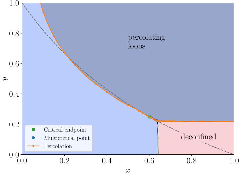
Our result for the percolation phase diagram is shown in Fig. 21 and explained in Sec. IX.3. Within our numerical precision, the percolation phase boundary matches the thermodynamic boundary of the deconfined phase along the entire Higgs transition line (to the right of the self-dual line), and passes through the self-dual critical point. (The percolation transition line also lies very close to the first order line, though closer examination indicates that these two lines do not entirely coincide, see App. D.)

The fact that the percolation line passes through the self-dual critical point agrees with the scenario in Ref. Huse and Leibler (1991). A far as we are aware, however, this result is not guaranteed a priori: the geometrical percolation transion could have separated from the Higgs transition at some point along the Higgs line, with the multicritical point lying in the interior of the percolating phase (see footnote).

It is also striking that the self-dual critical point lies on the percolation phase boundary despite having a very low fraction of occupied links, around $2.5\%$. Despite their low density, these links make up a scale-invariant ensemble of clusters. Fig. 22 shows the loops $\partial\mathcal{M}$ in an example configuration.

Figure 22: Loops in a sample of system size ${L=32}$ at ${x=0.6367}$. A spanning loop is highlighted in red (note periodic B.C.s). Our definition of a “loop” allows for junctions where 4 or 6 occupied links meet, but as can be seen they are relatively rare at the critical point.

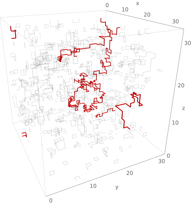
This scale invariance allows us to define a new exponent at the self-dual critical point, namely the fractal dimension $d_{f}$ of the critical loops. A priori, this exponent is independent of the scaling dimensions of local operators discussed above: ${d_{f}=3-x_{\text{conn}}}$ is determined by the scaling dimension $x_{\text{conn}}$ of a nonlocal geometrical operator of the type familiar from percolation Cardy (1996). Interestingly, though, our numerical result for $d_{f}$ below (Sec. IX.3),

$$d_{f}=1.77(2),$$ (37)

is consistent with $x_{\text{conn}}\overset{?}{=}x_{A}$, perhaps hinting at additional hidden symmetry structure at this critical point. (See Sec. X.1 for an argument that ${x_{A}\leq x_{\text{conn}}}$.)

IX.3 Percolation observables

We locate the boundary between percolating and short-loop (non-percolating) phases using the spanning probability, $P_{s}$. This is the probability that the sample contains a loop which spans the sample in a given axis direction. In the thermodynamic limit, this quantity converges to zero and to one in the nonpercolating and percolating phases respectively, and it is expected to take a universal value in between 0 and 1 at a continuous transition between the two phases.

We estimate the percolation phase boundary from crossings in $P_{s}$, plotted as a function of $y$, using small system sizes $L=8$, $12$ and $16$ (data not shown). We use larger sizes to analyse the transitions at $x=1$, at $y=1$, at the multicritical point and in the region around it. We may also obtain the correlation length exponent from a scaling collapse of $P_{s}$.

The phase diagram Fig. 21 shows three different phases. The deconfined phase has short loops, while the thermodynamically trivial phase splits into a percolating and a non-percolating phase (this is possible because the percolation transition need not have any thermodynamic signature). Note that here we are considering percolation of $e$ worldlines: the phase diagram for percolation of $m$ worldlines (in the dual membrane representation) may be obtained by duality.

As a check, we first examine the percolation transitions on the boundary of the phase diagram, where we expect to see standard universality classes (data in App. D). At $x=1$ results are as expected from the Ising mapping, with a fractal dimension consistent with the known value for critical Ising worldlines Winter et al. (2008); Kompaniets and Wiese (2020), and correlation length exponent consistent with the Ising value. At $y=1$, where the percolation transition is purely geometrical (has no thermodynamic signature) exponents are consistent with the standard 3D percolation universality class.

Figure 23: Scaling collapse of $P_{s}$ as a function of $(x-x_{c})L^{1/\nu}$ with $x_{c}=0.63666$ fixed. Inset: flow of $P_{s}$ as a function of the system size for several $x$ values close to the multicritical point, showing approximate scale invariance at $x=0.6367$.

Figure 24: Mass of the largest cluster (number of links) as a function of the system size at $x=0.6367$. The dashed line fits system sizes as a power-law $AL^{d_{f}}$, with $d_{f}=1.77(2)$.

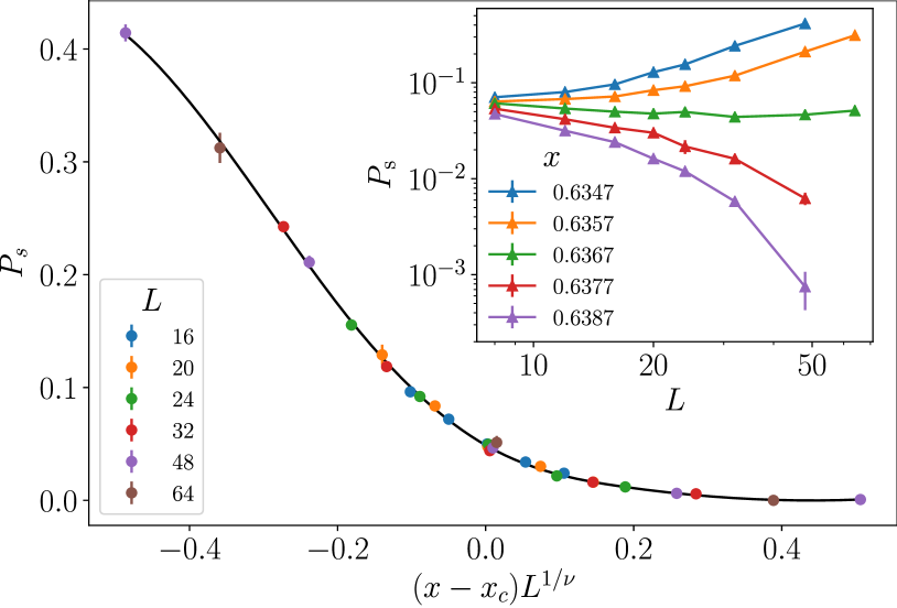
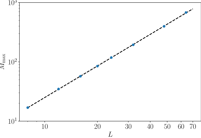
Fig. 23 shows data on the self-dual line, close to the self-dual critical point. The data are compatible with a critical point very close to ${x=0.6367}$ (inset of Fig. 23), i.e. with geometrical criticality coinciding with the self-dual critical point at the corner of the deconfined phase. A scaling collapse of $P_{s}$ as a function of $(x-x_{c})L^{1/\nu}$, leaving $x_{c}$ and $\nu$ free (not shown) gives $x_{c}=0.63664(10)$ and $\nu=0.69(6)$ compatible with our best estimates for the self-dual multicritical point. In Fig. 23, we show the scaling collapse when $x_{c}$ is fixed to our previous best estimate $x_{c}=0.636660$ (Sec. V.1). We use B-splines with 5 knots and obtain $\nu=0.70(6)$ for a fit that gives $\chi^{2}=27$ for 24 degrees of freedom. Using $\nu^{-1}=3-x_{S}$, this result for $\nu$ is consistent with our previous estimate of $x_{S}$, though with lower precision.

At the self-dual critical point, loops are fractal, and exist on all scales (Fig. 22). The fractal dimension $d_{f}$ can be estimated from fitting the total mass of the largest loop to a power-law in $L$, Fig. 24. The straight line fits the whole range of system sizes from 8 to 64, providing the estimate $d_{f}=1.77(2)$ quoted above.

X Related models

The previous section concludes our analysis of numerical data. We now consider some variations of the model, and relations to other models. Sec. X.1 connects the self-dual critical point to another partition function, for a “topologically constrained” ensemble of loops, which it may be interesting to study further. Sec. X.2 and Sec. X.3 discuss perturbations and crossovers in the gauge-Higgs model. Sec. X.4 discusses our numerical observation that the exponents $x_{A}$ and $x_{S}$ are close to exponents in the XY model.

X.1 An unusual self-dual loop model

In Sec. II.3 we considered a representation of the gauge-Higgs partition function as a “loop model”, for two species of “loops”, with a topological sign factor $(-1)^{\text{linking}}$ in the Boltzmann weight. In that model the two species of loops live on distinct cubic lattices. Here we consider a modified loop model in which the loops live on the same cubic lattice. This allows the partition function to be re-expressed in a form involving a topological constraint rather than a topological sign factor.

Let $\mathcal{C}_{e}$ and $\mathcal{C}_{m}$ be two species of loops on the cubic lattice. Here we define the allowed loop configurations differently to those in Sec. II.3: now we insist that the loops are strictly self-avoiding and mutually avoiding (a loop may visit a given site at most once, for example). With this definition the linking number $\hat{X}$ is well-defined.

The partition function is

$$Z_{\text{mod}}=4\sum_{\mathcal{C}_{e},\mathcal{C}_{m}}y^{|\mathcal{C}_{e}|}y^{\prime|\mathcal{C}_{m}|}(-1)^{\hat{X}(\mathcal{C}_{e},\mathcal{C}_{m})}.$$ (38)

($|\mathcal{C}_{e}|$ is the number of occupied links in $\mathcal{C}_{e}$, etc., and the loops in $\mathcal{C}_{e}\cup\mathcal{C}_{m}$ are mutually avoiding.) We do not yet know the full phase diagram of this new model, but it is plausible that it may also show a self-dual critical point, in the same universality class as the lattice gauge theory studied above.

As an aside, we note that the model could be varied in many ways. We could allow the “loops” to be clusters (as in the previous model, Eq. 5), by allowing the number of occupied links adjacent to a site to be any even number (rather than just 0 or 2 as in Eq. 38). With this choice the model maps on to the original gauge-Higgs model in the limit $y\rightarrow 0$ and in the limit $y^{\prime}\rightarrow 0$. This choice may have advantages for simulations (as may other choices of lattice as noted below). These changes do not affect the points we make here, so we consider the more easily-visualized ensemble of strictly self-avoiding loops.

Let $\mathcal{C}$ denote the full loop configuration, without regard to species labels, and let us specialize to the self-dual line where ${y=y^{\prime}}$:

$$Z_{\text{mod}}=4\sum_{\mathcal{C}}y^{|\mathcal{C}|}\sum_{\begin{subarray}{c}{\text{species}}\\ {\text{labels}}\end{subarray}}(-1)^{\hat{X}(\mathcal{C}_{e},\mathcal{C}_{m})}.$$ (39)

The final sum is over assignments of the loops in $\mathcal{C}$ to species $e$ or $m$, i.e. over splittings of $\mathcal{C}$ into $\mathcal{C}_{e}$ and $\mathcal{C}_{m}$. For simplicity, let us choose (non-periodic) boundary conditions such that loops cannot end on the boundary or wind around the system.

We can sum over the species assignments explicitly, for a fixed $\mathcal{C}$. The result is simple:

$$Z_{\text{mod}}=4\sum_{\mathcal{C}}y^{|\mathcal{C}|}\times 2^{(\text{\# loops in $\mathcal{C}$})}\times\chi_{\mathcal{C}}.$$ (40)

Here $\chi_{\mathcal{C}}=0,1$ depends only on the topology of $\mathcal{C}$, and simply imposes a restriction (constraint) on the allowed topologies. ${\chi_{\mathcal{C}}=1}$ so long as every loop in the configuration links with an even number of other loops, and ${\chi_{\mathcal{C}}=0}$ otherwise.

Strikingly, this expression is sign-free, and could be sampled with Monte-Carlo, using a local update that preserved the mod 2 total linking number of each loop. It would be interesting to know the phase diagram of this model or variants of it. (For an efficient numerical study, it might be useful to modify the lattice geometry of the model so that loops can form nontrivial links on a shorter lengthscale.)

This model also allows an interesting topological interpretation for correlation functions of the anti-self-dual operator.

In the ensemble (38), let us define the operator $\widetilde{A}(r)$ at a site $r$ to take the value $0$ if the site is not visited by a loop, $1$ if the site is visited by an $e$ loop, and $-1$ if the site is visited by an $m$ loop. This operator is odd under duality, so analogous to the operator $A(r)$ defined for the gauge-Higgs model in Sec. III.1.

By again explicitly summing over the loops’ species labels, we may write correlators of $\widetilde{A}$ in the formulation of Eq. 40. First, an insertion of $\widetilde{A}(r)$ forces a loop to pass through $r$. Second, the $\widetilde{A}(r)$ insertion forces the total linking number of this anchored loop (with other loops) to reverse its parity. In the original ensemble (40) every loop has even linking. In the presence of $\widetilde{A}$ insertions, the linking number of a loop that passes through an odd number of $\widetilde{A}$ operators must instead be odd (while the linking number of a loop that passes through an even number of $\widetilde{A}$ operators remains even).

Figure 25: Schematic: some of the configurations contributing to the correlator $\langle\widetilde{A}(r)\widetilde{A}(r^{\prime})\rangle$ in the model (40). Circles indicate locations $r$, $r^{\prime}$.

In Fig. 25 we illustrate some of the configurations that contribute to ${\langle\widetilde{A}(r)\widetilde{A}(r^{\prime})\rangle}$. For simplicity, we show the schematic situation at small $y$, where loop length is suppressed. The first term involves a single loop (with zero linking) that passes through both insertions. The other terms involve a chain of linked loops, with the loops at the two ends of the chain, passing through $r$ and $r^{\prime}$, having odd linking. (This picture shows that in the limit of small $y$ the correlation length $\xi$ for this correlator is proportional to ${|\ln y|^{-1}}$, since we must pay a factor of $y$ for every unit of loop length.) Moving away from the regime of small $y$, it remains true that there are two types of terms: those where the two $\widetilde{A}$ insertions lie on the same loop, and those where they lie on distinct loops which (unlike all the other loops in the configuration) have odd linking.

Assuming this model has a self-dual critical point, then this topological picture for ${\langle\widetilde{A}\widetilde{A}\rangle}$ yields an inequality for the fractal dimension $d_{f}$ of loops. This sheds some light on the coincidence of exponents that we found numerically in Sec. IX. Recall that the connectivity correlator, ${P_{\text{conn}}(r,r^{\prime})\sim r^{-2x_{\text{conn}}}}$, is the probability that two distant sites are connected by a loop. Above we have shown that these connected configurations are a subset of the configurations that contribute to ${\langle\widetilde{A}\widetilde{A}\rangle}$. That is, ${\langle\widetilde{A}\widetilde{A}\rangle=P_{\text{conn}}+R}$, where $R$ is the sum over the remaining configurations and is positive. Therefore

$$x_{A}\leq x_{\text{conn}},$$ (41)

or equivalently $d_{f}\leq 3-x_{A}$.

We expect that when the model above is perturbed away from the self-dual line, an Ising^∗ transition can take place, as in the original gauge-Higgs model. In the language of Eq. 38 this occurs in the same manner discussed in Sec. II.5: if one of the loop species has a finite typical size, it can be integrated out at large scales, leaving a simple ensemble of Ising-like worldlines (topologically unconstrained loops with a fugacity 1 per loop). It is also possible to see this crossover in the language of Eq. 40: adding the duality-breaking perturbation $\widetilde{A}$ relieves the topological linking constraint in Eq. 40 and leads to an ensemble where large loops have a fugacity of 1.

X.2 Perturbations of the gauge-Higgs model

After this detour, we return to the standard gauge-Higgs model to discuss some remaining questions.

We have characterized the leading self-dual and anti-self-dual scalar (spin-zero) operators at the self-dual critical point numerically, but it remains to characterize the subleading operators in these sectors, as well as operators with higher spin. One motivation for this is to formally determine the number of relevant scaling parameters once duality is broken, as we explain below.

On the appropriate line in parameter space, self-duality is an exact property of the standard gauge-Higgs model. But in many settings where the gauge-Higgs model is a useful effective theory, exact self-duality will be broken in the ultraviolet by additional interactions. It is natural to conjecture that the phase diagram structure in Fig. 1 can nevertheless survive, with self-duality appearing as an emergent symmetry at the corner of the deconfined phase, where Higgs and confinement transitions meet. In order for this to be the case, $A$ and $S$ should be the only relevant scalar operators at the self-dual critical point.

At first glance this is demonstrated by the fact that we only had to tune two parameters to reach this critical point. However this is not quite correct: the microscopic self-duality symmetry of the self-dual line forces all anti-self-dual perturbations to vanish there (not only the leading $A$ perturbation). Therefore, in principle we should separately check whether the subleading duality-odd scalar operator is relevant or irrelevant. Since $A$ itself has a large scaling dimension, we might expect that this subleading operator will be irrelevant, but this should be checked.

The subleading duality-even operator is irrelevant, but a sufficiently large duality-even perturbation may yield a “self-dual tricritical” point with an additional relevant direction.

In Ref. Dusuel et al. (2011) it was argued, using series expansions, that the toric code with $X$, $Y$ and $Z$ fields had a critical line, with varying exponents, in the $h_{x}=h_{z}$ plane. This will be interesting to investigate further, as continuously-varying exponents in 3D are rare. However, it should be noted that, in the present language, the perturbation $h_{y}$ breaks both internal and spatiotemporal symmetry. The toric code Hamiltonian with $h_{x}=h_{z}$, discussed in Sec. II.4, has a duality symmetry $D$ that we may take to be $X\rightarrow T(Z)$, $Z\rightarrow T(X)$, $Y\rightarrow-T(Y)$, where $T$ represents a translation by $(1/2,1/2)$. It also has an antiunitary time-reversal symmetry which we may take to act as ${X\rightarrow X}$, ${Z\rightarrow Z}$, ${Y\rightarrow-Y}$, ${i\rightarrow-i}$. Adding the $h_{Y}$ field breaks both of these symmetries. (It preserves their product.) It would be interesting to identify the leading continuum perturbation of the self-dual critical point that is induced by the $h_{y}$ coupling.

Recent work has demonstrated infinite-randomness scaling for a range of Higgs transitions in 2+1D quantum gauge theories with quenched disorder in the couplings Kang et al. (2020). It would be interesting to study the effect of disorder on the self-dual topological phase transition. The exponents $x_{S}$ and $x_{A}$ imply that spatially uncorrelated quenched disorder is a strongly relevant perturbation of the self-dual critical point in its 2+1D quantum manifestation, regardless of whether this disorder preserves duality or not.

X.3 Dimensional crossovers

Various dimensional crossover effects may also be worth studying. By making one of the three lattice directions finite and of width ${1/T\gg 1}$ (with periodic boundary conditions) we may study the effect of a low but nonzero temperature in the quantum problem Cardy (1996). Standard considerations show that on the boundaries of the phase diagram (at $y=0$ or $y^{\prime}=0$), the 3D Ising^∗ transitions give way to 2D Ising transitions, but that in the interior of the phase diagram these transitions become crossovers, with a finite correlation length Svetitsky (1986). This correlation length is exponentially large in $1/T$ at small $T$. In the worldline representation (5) this scaling is associated with closed worldlines of the massive anyon which are of length $1/T$ and wrap around the temporal cycle. (This exponential scaling may be why a numerical study of the $\mathbb{Z}_{2}$ gauge-Higgs model instead reported finite-temperature transitions Genovese et al. (2003).) A line of first-order transitions on the self-dual line will remain at small finite temperature. What happens to the self-dual critical point at nonzero temperature is less clear. The simplest possibility is that it becomes a conventional critical endpoint, so that the interior of the phase diagram contains only a first-order line, bounded by two conventional critical endpoints.

Other boundary condition choices for the finite dimension give other phase diagrams. For example, consider the loop model (5) in a slab geometry of thickness $\ell$, with open boundary conditions in the finite direction, with loop strands forbidden from terminating on the boundary. Physically this can be obtained by taking a 2D quantum system deep in the deconfined phase (corresponding to $y,y^{\prime}\ll 1$) and then varying the couplings inside a strip of width $\ell$ to allow anyons to proliferate there. Isolated strands that span the finite direction are now forbidden, so the mechanism that rendered the correlation length finite in the previous quasi-2D geometry is removed. Instead, after coarse-graining to scales $\gg\ell$ we may argue for an effective 2D loop model with two species of loops (and with no nontrivial topological sign factor). Away from the self-dual line, 2D Ising transitions are likely, associated with proliferation of a single loop species (a single anyon type). It may also be possible to have a gapless Ashkin-Teller-like regime on part of the self-dual line, where both species are critical.

If we think of the length-$\ell$ direction here as imaginary time instead of space, this setup may be related to the interesting finding of 2D Ashkin-Teller criticality in a deformed toric code wavefunction, for which equal-time correlators map to correlators in a 2D classical model Zhu and Zhang (2019). This deformed wavefunction is given by a finite-depth non-unitary circuit acting on the toric code wavefunction. This can be visualized in a path integral representation. In the zero-temperature path integral for the deconfined phase, the evolution for imaginary times $(-\infty,0)$ can be viewed as preparing the ground state ket and the evolution for times $(0,\infty)$ as preparing the corresponding bra. To obtain equal-time correlators in the deformed wavefunction, we insert a “slab” of finite temporal extent in between these two pieces, representing the action of the nonunitary circuit on bra and ket. This is reminiscent of the setup for the quasi-2D loop model above (since in the spactime region outside the slab we set $y=y^{\prime}=0$, meaning that, in the loop model picture, worldlines are forbidden except inside the slab).

It will also be interesting to characterize boundary critical phenomena, and conformally invariant boundary conditions, for the self-dual topological transition.

X.4 Comparison with XY exponents

A striking feature of our numerical results is that the values for scaling dimensions are close to certain values for the 3D XY universality class. Below we discuss why this is surprising.

At first sight (however, see below) a relationship with XY appears a natural guess Huse and Leibler (1991), by analogy with conventional ordering transitions, where two Ising critical lines (together with a first order line) can meet at an XY critical point. Given two conventional Ising-like order parameters $\varphi_{x}$ and $\varphi_{y}$, and an additional $\mathbb{Z}_{2}$ symmetry that exchanges them, XY criticality for ${{\bm{\mathbf{\varphi}}}=(\varphi_{x},\varphi_{y})}$ can arise by tuning one parameter because the symmetry-allowed “cubic” anisotropy ${\varphi_{x}^{4}+\varphi_{y}^{4}-6\varphi_{x}^{2}\varphi_{y}^{2}}$ is a (weakly) irrelevant operator at the XY fixed point Pujari et al. (2015); Shao et al. (2020).

In the present model, we know that the Ising^∗ lines can be understood as ordering transitions for “fictitious” (non-gauge invariant) Ising-like order parameters. Therefore at first sight it is tempting to make the above analogy. We would then identify the operator $S$ with the thermal operator ${{\bm{\mathbf{\varphi}}}^{2}}$, and the operator $A$ with the symmetry-breaking mass operator ${\varphi_{x}^{2}-\varphi_{y}^{2}}$. The scaling dimensions of these operators in the XY model are ${x_{\bm{\mathbf{\varphi}}^{2}}=1.51136(22)}$) and ${x_{\varphi_{x}^{2}-\varphi_{y}^{2}}=1.23629(11)}$ Chester et al. (2020); Hasenbusch and Vicari (2011); Hasenbusch (2019). Strikingly, the differences between these values and our results for $x_{S}$ and $x_{A}$ in Tab. 1 are small, comparable in size with the (statistical) error bars quoted in the table.

The problem with this analogy is that it ignores the nontrivial mutual statistics between $e$ and $m$ excitations Vidal et al. (2009); Tupitsyn et al. (2010); Geraedts and Motrunich (2012a) that are the key feature of the transition. These mutual statistics do not affect critical exponents on the Ising^∗ lines, because only one of the two excitations is massless on these lines. But both excitations become massless at the self-dual critical point.

For example, any consistent description of the fixed point should correctly reproduce the spectrum of low-lying anyonic quasiparticles that exists when we perturb slightly away from the self-dual critical point, into the deconfined phase. It is hard to see how this could be consistent with a mapping that related the present fixed point and the XY fixed point.

The obstacle to making a connection with XY can also be seen in the geometrical pictures. In the membrane picture, the possibility of defining a fictitious Ising order parameter is associated with the membranes being effectively closed on large scales, as discussed in Sec. IX. But at the self-dual critical point, we have “holes” in these membranes on all scales, as we have demonstrated explicitly. Therefore the attempt to make a connection with a simple Landau theory, at least in this manner, fails at this critical point.

It therefore seems likely that the exponents $x_{A}$ and $x_{S}$ at the self-dual critical point are numerically close to XY exponents, but distinct from them. If on the other hand the exponents are the same as those of the XY fixed point, this relationship between a topological phase transition and a simple ordering transition would have to be of a fundamentally new kind. We plan to return to these questions elsewhere.

XI Outlook

The three-dimensional $\mathbb{Z}_{2}$ gauge-Higgs model is the simplest nontrivial lattice gauge theory Wegner (1971); Wilson (1974); Balian et al. (1974); Fradkin and Shenker (1979); Tupitsyn et al. (2010); Wu et al. (2012); Vidal et al. (2009). Its remarkable duality property allows for a self-dual topological phase transition whose properties have long been unresolved. We have given direct evidence for scale invariance at this transition, exploring system sizes up to two orders of magnitude larger than the lattice spacing. Exciting directions remain open, on the computational, experimental, and theoretical fronts.

First, there are many intriguing questions that could be addressed using further simulations. At the basic level, armed with the accurate estimate of $x_{c}$, further characterization of the critical point will be possible, examining the scaling dimensions of a wider range of operators (Sec. X.2), and pinning down OPE coefficients more precisely (Sec. VII).

We have also proposed new models that could be simulated. The loop model in Sec. X.1 has a simplified action of self-duality. It has a sign-free reformulation of a nonstandard kind, as an ensemble of loops with a simple “topological constraint”. (This connects, heuristically, to the longstanding question from polymer physics of how to think about the renormalization group for models with topological constraints Edwards (1977); De Gennes and Gennes (1979); des Cloizeaux (1981); Khokhlov and Nechaev (1985); Rubinstein (1986); Cates and Deutsch (1986); Halverson et al. (2014); Imakaev et al. (2015); Serna et al. (2015); Dai and Nahum (2020).) This sign-free formulation could be exploited to determine the model’s phase diagram, and may suggest a more general strategy for obtaining sign-free lattice models for topological transitions.

In the context of the standard lattice gauge theory, a range of perturbations and crossovers may be studied (Sec. X.2 and Sec. X.3), for example to search for self-dual tricriticality.

The self-dual topological phase transition can be viewed as a paradigmatic challenge for Monte Carlo algorithm design. Although it is Monte-Carlo sign-free (unlike many other lattice gauge theories De Forcrand (1995); Peardon (2002); Schaefer (2011); Ishikawa (2009)), the lack of a nonlocal cluster update Newman et al. for ensembles of membranes, and the large dynamical exponent (Sec. VIII), make it expensive to simulate. Creative algorithmic improvements would be valuable. We might consider updates acting on larger finite clusters, perhaps optimized using machine learning Liu et al. (2017); Huang and Wang (2017).

If we are in the deconfined phase, but close to the self-dual critical point, various features of the spectrum of massive quasiparticles Vidal et al. (2009); Dusuel et al. (2011) will be universal and could perhaps be examined using Monte Carlo Suwa et al. (2016), series expansion Vidal et al. (2009); Dusuel et al. (2011) or tensor network techniques Vanderstraeten et al. (2015, 2019). For example, does the fermionic $\epsilon$ excitation exist as a stable bound state in this regime, or inevitably decay into an $e$ and an $m$?

Even away from the self-dual point, interesting questions remain. The existence of “fictitious” Ising order parameters on the Higgs and confinement transition lines is the key to the theoretical understanding of these transitions Wegner (1971); Fradkin and Shenker (1979); Huse and Leibler (1991); Gregor et al. (2011). We have argued that we can construct these field configurations explicitly by a quasi-local patching process in the membrane representation of the partition function, so that for example the Ising “two-point function” $G(r,r^{\prime})$ can be computed numerically. Formally, this is the expectation value of a dressed string operator that extends from $r$ to $r^{\prime}$ (Sec. IX). In separate work we will analyze the emergence of this structure in more detail Nahum et al. .

The self-dual critical point may be accessible experimentally, either in its 3D classical or its ${2+1\mathrm{D}}$ quantum manifestation. It would be exciting to see the full structure of the gauge-Higgs phase diagram, with the meeting of the two Ising^∗ lines, in experiments on amphiphilic membranes (verifying a longstanding conjecture Huse and Leibler (1991)). In order to access this point, the membranes must have free edges, i.e. a nonempty membrane boundary $\partial\mathcal{M}$. However, by analogy with results in App. B, the required density of free edges may be relatively small.

Strategies for quantum simulation of lattice gauge theories are under intensive development Dalmonte and Montangero (2016); Zohar et al. (2017a, b); Schweizer et al. (2019); Barbiero et al. (2019); Bañuls and Cichy (2020); Davoudi et al. (2020); Cui et al. (2020); Paulson et al. (2020), so it may one day be possible to explore the self-dual critical point and its real-time quantum dynamics experimentally.

Perplexing theoretical questions remain. Why are our estimates for $x_{A}$ and $x_{S}$ so close to XY values (Sec. X.4)? Further numerical characterizations of the critical point mentioned above may shed light on this. Significant input may also come from the conformal bootstrap Poland et al. (2019); El-Showk et al. (2012); Kos et al. (2014, 2016); Poland et al. (2019), by exploring the space of theories with the requisite $\mathbb{Z}_{2}$ symmetry.

There remains the fundamental question that we started with: can we formulate a useful continuum field theory for the self-dual topological transition? Criteria for “usefulness” could include the possibility of calculating exponents in a systematic expansion, as well as the possibility of deriving the structure of phase diagram analytically. More generally, the time seems ripe for a numerical and theoretical attack on phase transitions where multiple species of anyons, with nontrivial statistics, simultaneously condense Vidal et al. (2009); Tupitsyn et al. (2010); Geraedts and Motrunich (2012a); Burnell (2018).

Appendix A Membrane representation of $Z$

We now review the standard relationship between the Ising gauge theory partition function and partition functions for membranes on either the original cubic lattice or its dual Huse and Leibler (1991). In the interpretation as a 2D quantum system in imaginary time, these membranes are worldsurfaces of either electric or magnetic strings (cf. Fig. 5), depending on whether we use the original lattice or the dual lattice. In general the strings (which live in a 2D spatial plane) can be open lines, terminating at $e$ or $m$ particles in the respective cases. Therefore the membranes (which live in 3D spacetime) are not closed in general, but rather have boundaries, which are the wordlines of $e$ or $m$ particles respectively. The “action” of a given membrane configuration (the logarithm of the Boltzmann weight) is, up to constants, the area of the worldsurfaces plus the length of the worldlines.

A.1 Membranes on the original lattice

Using the fact that the variables take only the values $\pm 1$, $Z$ in Eq. 1 can be rewritten in a form convenient for a standard graphical expansion:

$$Z(x,y)\equiv\frac{1}{2^{4L^{3}}}\sum_{\{\sigma\},\{\tau\}}\prod_{\square}\left(1+x\prod\sigma\right)\prod_{\ell}\left(1+y\sigma\tau\tau\right),$$ (42)

with ${K=\frac{1}{2}\ln\frac{1+x}{1-x}}$ and ${J=\frac{1}{2}\ln\frac{1+y}{1-y}}$. We expand out the products over (1) plaquettes $\square$ and (2) links $\ell$ in Eq. 42, and represent a given term by colouring plaquettes of the lattice and highlighting links in bold, as in Fig. 3. A plaquette is coloured (“occupied”) iff we pick the “$x\prod\sigma$” term for that plaquette and similarly a link is bold if we pick the “$y\sigma\tau\tau$” term. For a given term in the expansion, the collection of occupied plaquettes constitutes the membrane configuration $\mathcal{M}$.

Now for each term we must sum over $\sigma$ and $\tau$. The term will vanish if there is any link $\ell$ where the terms we have chosen contribute $\sigma_{\ell}$ an odd number of times in total. This means that the set of bold links must coincide with the membrane boundary $\partial\mathcal{M}$ to have a nonvanishing term ($\partial\mathcal{M}$ is defined as the set of links where an odd number of coloured plaquettes meet). If this is satisfied, then the sums over $\sigma$ and $\tau$ are both nonvanishing, giving trivial factors $2^{3L^{3}}$ and $2^{L^{3}}$ respectively that cancel the normalization term chosen in Eq. 42. We are left with the partition function as sum over membrane configurations weighted by $x^{|\mathcal{M}|}y^{|\partial\mathcal{M}|}$, Eq. 3.

From this expansion we also see that the face and edge operators defined in Sec. III may be written as

$$\mathcal{F}(p) =\frac{x}{1-x^{2}}\left(\prod\sigma-x\right), \mathcal{E}(\ell) =\frac{y}{1-y^{2}}\left(\sigma\tau\tau-y\right),$$ (43)

for a plaquette $p$ and link $\ell$ respectively.

The expansion above is the standard high-temperature expansion, meaning that terms are weighted by powers of the “fugacities” $x$ and $y$ which are small when $K$ and $J$ are small. Since the lattice is finite the expansion may be done exactly, to all orders: i.e. one may think of it as a reformulation of the partition function and not as a perturbative series. It is a generalization of the high-temperature expansion of the Ising model, which would obtain if the $\sigma$ field was absent and we just had loops associated with $y\tau\tau$.

A.2 Membranes on the dual lattice

Eq. 42 can be related to membranes on the dual lattice even more directly.

Let us choose the gauge $\tau=1$ so that the partition function is a sum over only the $\sigma=\pm 1$ on each link. We can represent a given term by a collection of occupied links, where a link $\ell$ is occupied iff ${\sigma_{\ell}=-1}$. (Note that this notion of a link being occupied is unrelated to the one in the previous subsection.) Next, recall that plaquettes of the dual lattice are in 1:1 correspondence with links of the original lattice, so a configuration of occupied links is equivalent to a configuration of occupied plaquettes $\widetilde{\mathcal{M}}$ on the dual lattice. What is the Boltzmann weight of $\widetilde{\mathcal{M}}$? Each occupied plaquette costs ${x^{\prime}\equiv(1-y)/(1+y)}$ (from the ratio of the ${1+y\sigma}$ term in Eq. 42 with ${\sigma=-1}$ to that with ${\sigma=+1}$). Further a link of the dual lattice where an odd number of occupied plaquettes meet means a square on the original lattice where $\prod\sigma=-1$. So each link in $\partial\widetilde{\mathcal{M}}$ contributes ${y^{\prime}\equiv(1-x)/(1+x)}$. Including the normalization,

$$Z(x,y)=\frac{(1+x)^{3L^{3}}(1+y)^{3L^{3}}}{2^{3L^{3}}}\sum_{\widetilde{\mathcal{M}}}\,{x^{\prime}}^{|\widetilde{\mathcal{M}}|}\,{y^{\prime}}^{|\partial\widetilde{\mathcal{M}}|}.$$ (44)

A.3 Manifestly self-dual representation

Next we demonstrate the reformulation in terms of two species of loops (or more precisely, clusters), cf. Fig. 4.

In addition to the degrees of freedom $\sigma$ and $\tau$ on the links and sites (respectively) of the original lattice, let us add degrees of freedom $\tilde{\sigma}$ and $\tilde{\tau}$ on the links and sites of the dual lattice. Let us denote the links of the original lattice by $\mathcal{L}$ and those of the dual lattice by $\widetilde{\mathcal{L}}$. Define

$$Z^{\prime}= \sum_{\sigma,\tau,\tilde{\sigma},\tilde{\tau}}e^{-S_{\text{top}}[\sigma,\widetilde{\sigma}]}\prod_{\ell\in\mathcal{L}}\left(1+y\sigma\tau\tau\right)\prod_{\tilde{\ell}\in\widetilde{\mathcal{L}}}\left(1+y^{\prime}\tilde{\sigma}\tilde{\tau}\tilde{\tau}\right).$$ (45)

The “topological” action $S_{\text{top}}[\sigma,\widetilde{\sigma}]$ is both gauge invariant and symmetric between $\sigma$ and $\tilde{\sigma}$: $e^{-S_{\text{top}}}=(-1)^{\hat{X}}$, where $\hat{X}$ is the $\mathbb{Z}_{2}$ linking number of the flux lines of $\sigma$ with those of $\tilde{\sigma}$. However it is convenient here to define it as

$$e^{-S_{\text{top}}}=\prod_{\tilde{\ell}\in\widetilde{\mathcal{L}}}\left(\delta_{\tilde{\sigma}_{\tilde{\ell}},1}+\delta_{\tilde{\sigma}_{\tilde{\ell}},-1}\prod\sigma\right)$$ (46)

where these properties are not manifest.

To see the equivalence to the original Ising gauge theory (42) we simply pick the gauge $\tilde{\tau}=1$ and do the sum on $\tilde{\sigma}$ separately for each link,

$$\sum_{\tilde{\sigma}}\left(\delta_{\tilde{\sigma}_{\tilde{\ell}},1}+\delta_{\tilde{\sigma}_{\tilde{\ell}},-1}\prod\sigma\right)(1+y^{\prime}\tilde{\sigma})=(1+y^{\prime})\left(1+x\prod\sigma\right),$$ (47)

so that

$$Z^{\prime}=2^{L^{3}}(1+y^{\prime})^{3L^{3}}\sum_{\{\sigma\},\{\tau\}}\prod_{\square}\left(1+x\prod\sigma\right)\prod_{\ell}\left(1+y\sigma\tau\tau\right).$$ (48)

To obtain the expression in terms of $\mathcal{C}_{e}$ and $\mathcal{C}_{m}$ in Eq. 5 we first perform the graphical expansion of the two products in (45), giving the sum over “loop” configurations $\mathcal{C}_{e}$ and $\mathcal{C}_{m}$ (Fig. 4). In addition to the fugacities $y$ and $y^{\prime}$ these are weighted by

$$\sum_{\sigma,\tilde{\sigma}}e^{-S_{\text{top}}}\left(\prod_{\ell\in\mathcal{C}_{e}}\sigma_{\ell}\right)\left(\prod_{\tilde{\ell}\in\mathcal{C}_{m}}\tilde{\sigma}_{\tilde{\ell}}\right)=2^{(4L^{3}+2)}(-1)^{X(\mathcal{C}_{e},\mathcal{C}_{m})}.$$ (49)

We can see this by using (46) to make a graphical expansion of the left hand side above, in terms of a membrane configuration $\mathcal{M}$ on the original lattice with boundary ${\partial\mathcal{M}=\mathcal{C}_{e}}$. For a given term in the expansion, the $\tilde{\sigma}$ are fixed by the Kronecker deltas, which dictates the sign of the product $\prod_{\tilde{\ell}\in\mathcal{C}_{m}}\tilde{\sigma}$ on the LHS of (49). There are, for periodic boundary conditions, $2^{L^{3}+2}$ choices of $\mathcal{M}$ for fixed ${\partial\mathcal{M}=\mathcal{C}_{e}}$, but they all give the same sign. Altogether,

$$Z^{\prime}=2^{(6L^{3}+2)}\sum_{\mathcal{C}_{e},\,\mathcal{C}_{m}}(-1)^{X(\mathcal{C}_{e},\mathcal{C}_{m})}y^{|\mathcal{C}_{e}|}{y^{\prime}}^{|\mathcal{C}_{m}|}.$$ (50)

Summarizing, $Z^{\prime}$ can be related to $Z$ in Eqs. 3, 42 by

$$Z=4\,c\sum_{\mathcal{C}_{e},\,\mathcal{C}_{m}}(-1)^{X(\mathcal{C}_{e},\mathcal{C}_{m})}y^{|\mathcal{C}_{e}|}{y^{\prime}}^{|\mathcal{C}_{m}|},$$ (51)

where ${c=2^{L^{3}}\left(1+y^{\prime}\right)^{-3L^{3}}=2^{-2L^{3}}\left(1+x\right)^{3L^{3}}}$.

Appendix B First-order coexistence

Although we have concentrated our study on the vicinity of the multicritical point, we can extract from the data some information related to the first-order coexistence region along the self-dual line. Starting from the deconfined phase (large $x$) this region starts at the multicritical point, $x_{c}$, and ends at a critical endpoint, $x_{\mathrm{cep}}$. The estimate $x_{c}\approx 0.6367$ was obtained in Secs. IV and V. The location of $x_{\mathrm{cep}}$ is, in principle, easier to determine because in this region $\operatorname{b}_{4}(A)$ (defined in Eq. 21) behaves monotonically and presents a crossing, as shown in Fig. 26. From the figure we roughly estimate $x_{\mathrm{cep}}\approx 0.605$. Though this is a rough estimate, it is worth noting that the value of $\operatorname{b}_{4}(A)$ at the crossing point is consistent with standard Ising universality (as for the liquid-gas critical endpoint), for which ${\operatorname{b}_{4}(A)\approx 0.7}$ Ferrenberg et al. (2018).

Figure 26: $\operatorname{b}_{4}(A)=-(1/2)\kappa_{4}(A)/{\rm Var}(A)^{2}$ as a function of $x$ for three system sizes. The lines are cubic polynomial fits.

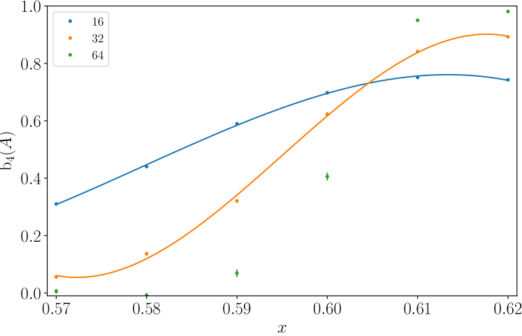
In between $x_{c}$ and $x_{\mathrm{cep}}$, histograms of $A$ or of the total membrane Area or membrane boundary Length have two peaks, corresponding to the two coexisting phases. For large system sizes our MC scheme will not properly sample both minima, so it could become hard to obtain equations of state for each phase. However, we can exploit the symmetry properties of $A$ and $S$. Denoting expectation values in the two equilibria by ${\left\langle\ldots\right\rangle_{\pm}}$, in the thermodynamic limit we have ${\left\langle A\right\rangle_{\pm}=\pm\left\langle|A|\right\rangle}$. Therefore by Eqs. 9 and 10,

$$\frac{\left\langle\mathrm{Area}\right\rangle_{\pm}}{3L^{3}} =\frac{\pm\left\langle|A|\right\rangle+\left\langle S\right\rangle}{12}$$ (52)

$$\frac{\left\langle\mathrm{Length}\right\rangle_{\pm}}{3L^{3}} =\frac{1-x^{2}}{2x}\frac{\pm\left\langle|A|\right\rangle-\left\langle S\right\rangle}{12}+\frac{1-x}{2},$$ (53)

on the coexistence region of the self-dual line and in the thermodynamic limit. These equations give equations of state for each phase. The results are shown in Figs. 27.

Figure 27: Top: Average plaquette occupation number versus $x$ obtained from $\left\langle|A|\right\rangle$ and $\left\langle S\right\rangle$ on the self-dual line (see text). The limits of these curves as $L\rightarrow\infty$ give the two equations of state for the two coexisting phases. The colors in the legend indicate different system sizes. The dashed black line is the average of the two coexisting phases, determined by $\left\langle A\right\rangle=0$, and the black stars indicate the locations of $x_{\mathrm{cep}}$ and $x_{c}$ (${x_{\mathrm{cep}}<x_{c}}$). Lines are just a guide to the eye. Bottom: Similarly for the average link occupation number.

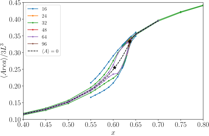
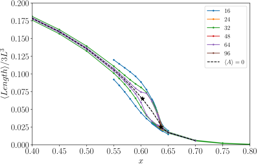
Appendix C Details of MC scheme and of fits

For most of our simulations, each MC step consists in updating all of the plaquettes (taking each of the three orientations in turn) and then updating all of the cubes. To allow parallelization we divide plaquettes parallel to the $(x,y)$ plane into 2 sublattices, and similarly for plaquettes in the $(y,z)$ and $(x,z)$ planes. We also divide cubes into two sublattices. We used one MC step as our unit of time. We studied system sizes up to $L=96$ and our longest simulations had $4\times 10^{9}$ MC steps. Error bars for cumulants of $A$ and $S$ are calculated using bootstrap methods Newman et al. (for this purpose the correlation time is estimated as the time for the correlation to decay by a factor of 10).

For the fits in Sec. V the scaling functions were described using B-splines with 8 to 12 degrees of freedom. The data used for the fits were restricted to ${x\in[0.633,0.640]}$ and to scaling variable $z\in[-0.5,0.5]$, although the particular intervals could slightly change from fit to fit. The system sizes included correspond to the best statistical fit, in the sense that the $p$-value (probability of getting a $\chi^{2}$ value below the one obtained from the fit, for the degrees of freedom used) was maximized.

Appendix D Further percolation data

D.1 Percolation at the Ising^∗ transition ($x=1$)

The transition at $x=1$ maps to 3D Ising. Up to a difference in boundary conditions, the wordlines are those in a standard high-temperature expansion of the Ising model, and the percolation transition happens precisely at the Ising critical point for the cubic lattice, $y=0.21809$. We indeed find that curves for the spanning probability $P_{s}$ cross close to this value, and can be collapsed by plotting as a function of $(y-y_{c})L^{1/\nu}$, using known Ising critical values, $y_{c,I}=0.21809$ and $\nu_{I}=0.63012$ Winter et al. (2008), Fig. 28. We also check that the mass of the largest loop (number of links, $M_{\mathrm{max}}$) follows a power-law with a fractal dimension consistent with the known value $d_{f,I}=1.7349(65)$ for Ising worldlines Winter et al. (2008). The inset of Fig. 28 shows $M_{\mathrm{max}}$ as a function of the system size at $y=0.218$.

Figure 28: Main Panel: scaling collapse of $P_{s}$ as a function of $(y-y_{c,I})L^{1/\nu_{I}}$, for $x=1$, with ${y_{c,I}=0.21809}$ and ${\nu_{I}=0.63012}$. Inset: $M_{\mathrm{max}}$ as function of the system size $L$ at $x=1,\,y=0.218$. Straight-line shows a power-law using the fractal dimensions of Ising worldlines ${d_{f,I}=1.7349}$.

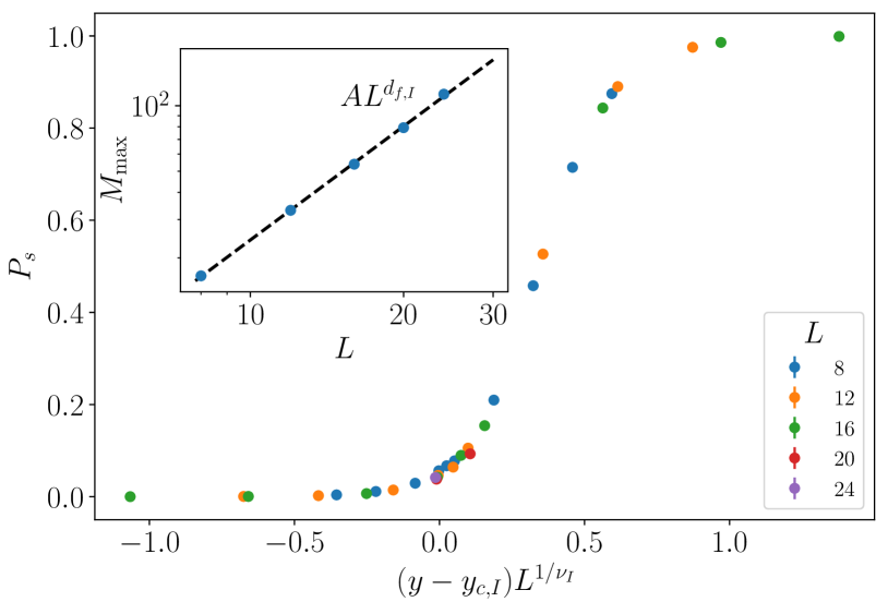
D.2 Percolation on the $y=1$ boundary

When the percolation transition takes place in within the thermodynamically trivial phase we expect conventional percolation universality. As an example we consider the case $y=1.$ An attempt to obtain scaling collapse of $P_{s}$ suggests that finite size effects are important for this range of system sizes. Fig. 29 shows an attempt at scaling collapse using $\nu_{P}=0.8762$ Xu et al. (2014). An estimate of the fractal dimension of the loops from $M_{\text{max}}$ (inset to Fig. 29) gives $d_{f}=2.56$ (to be compared with 2.53 for the percolation universality class).

Figure 29: Main Panel: scaling collapse of $P_{s}$ as a function of $(x-x_{cP})L^{1/\nu_{P}}$, for $y=1$, with $x_{cP}=0.0865$ and $\nu_{P}=0.8762$ Inset: $M_{\mathrm{max}}$ as function of the system size $L$ at at $x=0.087$. Straight line shows power-law with fractal dimension of percolation universality class, $d_{f,P}=2.53$.

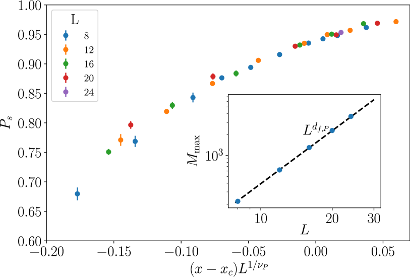
D.3 Percolation on the self-dual line

The phase diagram Fig. 21 in the main text shows that we encounter several percolation transitions as we move along the self-dual line. We have shown data close to the self-dual critical point $x_{c}$ in the main text. For smaller $x$ we encounter the first-order line where two phases coexist, one with $A>0$ and one with $A<0$. To separate the properties of the two coexisting phases, we may average $P_{s}$ separately for configurations with $A>0$ and $A<0$. The phase with $A>0$ appears to percolate throughout the entire range of the first-order line. Therefore the phase with $A<0$ must also percolate for some region of the first-order line close to the critical endpoint (since the two phases become identical there). One possibility (at first sight the more natural) is that the phase with $A<0$ undergoes a percolation transition at some intermediate $x$ lying on the interior of the first-order line. Another possibility is that this transition is pushed all the way to $x_{c}$, with the $A<0$ phase having an extremely weak but nonzero percolation order parameter for $x\lesssim x_{c}$. Data for small sizes do not allow us to determine which of these occurs.

References

- Fisher (1974) Michael E. Fisher, “The renormalization group in the theory of critical behavior,” Rev. Mod. Phys. 46, 597–616 (1974).
- Sachdev (2007) Subir Sachdev, “Quantum phase transitions,” Handbook of Magnetism and Advanced Magnetic Materials (2007).
- Wegner (1971) Franz J Wegner, “Duality in generalized ising models and phase transitions without local order parameters,” Journal of Mathematical Physics 12, 2259–2272 (1971).
- Kosterlitz and Thouless (1973) John Michael Kosterlitz and David James Thouless, “Ordering, metastability and phase transitions in two-dimensional systems,” Journal of Physics C: Solid State Physics 6, 1181 (1973).
- de Gennes (1972) Pierre-Gilles de Gennes, “Exponents for the excluded volume problem as derived by the wilson method,” Physics Letters A 38, 339–340 (1972).
- Huse and Leibler (1991) David A Huse and Stanislas Leibler, “Are sponge phases of membranes experimental gauge-higgs systems?” Physical review letters 66, 437 (1991).
- Lammert et al. (1993) Paul E Lammert, Daniel S Rokhsar, and John Toner, “Topology and nematic ordering,” Physical review letters 70, 1650 (1993).
- Francesco et al. (2012) Philippe Francesco, Pierre Mathieu, and David Sénéchal, Conformal field theory (Springer Science & Business Media, 2012).
- Fradkin (2013) Eduardo Fradkin, Field theories of condensed matter physics (Cambridge University Press, 2013).
- Senthil et al. (2004) Todadri Senthil, Ashvin Vishwanath, Leon Balents, Subir Sachdev, and Matthew PA Fisher, “Deconfined quantum critical points,” Science 303, 1490–1494 (2004).
- Fradkin and Shenker (1979) Eduardo Fradkin and Stephen H Shenker, “Phase diagrams of lattice gauge theories with higgs fields,” Physical Review D 19, 3682 (1979).
- Jongeward et al. (1980) Gary A Jongeward, John D Stack, and C Jayaprakash, “Monte carlo calculations on z 2 gauge-higgs theories,” Physical Review D 21, 3360 (1980).
- Tupitsyn et al. (2010) IS Tupitsyn, Alexei Kitaev, NV Prokof’Ev, and PCE Stamp, “Topological multicritical point in the phase diagram of the toric code model and three-dimensional lattice gauge higgs model,” Physical Review B 82, 085114 (2010).
- Vidal et al. (2009) Julien Vidal, Sébastien Dusuel, and Kai Phillip Schmidt, “Low-energy effective theory of the toric code model in a parallel magnetic field,” Physical Review B 79, 033109 (2009).
- Kogut (1979) John B Kogut, “An introduction to lattice gauge theory and spin systems,” Reviews of Modern Physics 51, 659 (1979).
- Read and Chakraborty (1989) N Read and B Chakraborty, “Statistics of the excitations of the resonating-valence-bond state,” Physical Review B 40, 7133 (1989).
- Kivelson (1989) Steven Kivelson, “Statistics of holons in the quantum hard-core dimer gas,” Physical Review B 39, 259 (1989).
- Read and Sachdev (1991) N Read and Subir Sachdev, “Large-n expansion for frustrated quantum antiferromagnets,” Physical review letters 66, 1773 (1991).
- Wen (1991) Xiao-Gang Wen, “Mean-field theory of spin-liquid states with finite energy gap and topological orders,” Physical Review B 44, 2664 (1991).
- Senthil and Fisher (2000) T Senthil and Matthew PA Fisher, “Z 2 gauge theory of electron fractionalization in strongly correlated systems,” Physical Review B 62, 7850 (2000).
- Moessner et al. (2001) Roderich Moessner, Shivaji L Sondhi, and Eduardo Fradkin, “Short-ranged resonating valence bond physics, quantum dimer models, and ising gauge theories,” Physical Review B 65, 024504 (2001).
- Kitaev (2003) A Yu Kitaev, “Fault-tolerant quantum computation by anyons,” Annals of Physics 303, 2–30 (2003).
- Balian et al. (1974) Roger Balian, JM Drouffe, and Claude Itzykson, “Gauge fields on a lattice. i. general outlook,” Physical Review D 10, 3376 (1974).
- Wu et al. (2012) Fengcheng Wu, Youjin Deng, and Nikolay Prokof’ev, “Phase diagram of the toric code model in a parallel magnetic field,” Physical Review B 85, 195104 (2012).
- Huse and Leibler (1988) D A Huse and S Leibler, “Phase behaviour of an ensemble of nonintersecting random fluid films,” J. Phys. (Paris) 49, 605 (1988).
- Cates et al. (1988) ME Cates, D Roux, D Andelman, ST Milner, and SA Safran, “Random surface model for the l3-phase of dilute surfactant solutions,” EPL (Europhysics Letters) 5, 733 (1988).
- David (1989) Francois David, “O (n) gauge models and self-avoiding random surfaces in three dimensions,” EPL (Europhysics Letters) 9, 575 (1989).
- Roux et al. (1990) D Roux, ME Cates, U Olsson, RC Ball, F Nallet, and AM Bellocq, “Light scattering from a surfactant “sponge” phase: Evidence for a hidden symmetry,” EPL (Europhysics Letters) 11, 229 (1990).
- Roux et al. (1992) D Roux, C Coulon, and ME Cates, “Sponge phases in surfactant solutions,” The Journal of Physical Chemistry 96, 4174–4187 (1992).
- Roux (1995) Didier Roux, “Sponge phases: An example of random surfaces,” Physica A: Statistical Mechanics and its Applications 213, 168–172 (1995).
- (31) L Peliti, ““amphiphilic membranes”, in “fluctuating geometries in statistical mechanics and field theory”, f. david, p. ginsparg, j. zinn-justin, (eds.) les houches, session lxii, 1994 (amsterdam: Elsevier, 1996) 195-285,” .
- Nandkishore et al. (2012) Rahul Nandkishore, Max A Metlitski, and T Senthil, “Orthogonal metals: The simplest non-fermi liquids,” Physical Review B 86, 045128 (2012).
- Kapustin and Thorngren (2017) Anton Kapustin and Ryan Thorngren, “Higher symmetry and gapped phases of gauge theories,” in Algebra, Geometry, and Physics in the 21st Century (Springer, 2017) pp. 177–202.
- Gaiotto et al. (2015) Davide Gaiotto, Anton Kapustin, Nathan Seiberg, and Brian Willett, “Generalized global symmetries,” Journal of High Energy Physics 2015, 172 (2015).
- Wen (2019) Xiao-Gang Wen, “Emergent anomalous higher symmetries from topological order and from dynamical electromagnetic field in condensed matter systems,” Physical Review B 99, 205139 (2019).
- (36) M.E.J. Newman, G.T. Barkema, and I.T.P.G.T. Barkema, Monte Carlo Methods in Statistical Physics.
- Geraedts and Motrunich (2012a) Scott D Geraedts and Olexei I Motrunich, “Monte carlo study of a u (1) u (1) system with -statistical interaction,” Physical Review B 85, 045114 (2012a).
- Burnell (2018) Fiona J Burnell, “Anyon condensation and its applications,” Annual Review of Condensed Matter Physics 9, 307–327 (2018).
- Geraedts and Motrunich (2012b) Scott D Geraedts and Olexei I Motrunich, “Phases and phase transitions in a u (1) u (1) system with = 2 /3 mutual statistics,” Physical Review B 86, 045106 (2012b).
- Lee et al. (2016) Jong Yeon Lee, Scott Geraedts, and Olexei I Motrunich, “Monte carlo study of phase transitions out of symmetry-enriched topological phases of bosons in two dimensions,” Physical Review B 93, 035103 (2016).
- Geraedts and Motrunich (2012c) Scott D Geraedts and Olexei I Motrunich, “Line of continuous phase transitions in a three-dimensional u (1) loop model with 1/r 2 current-current interactions,” Physical Review B 85, 144303 (2012c).
- Levin and Senthil (2004) Michael Levin and Todadri Senthil, “Deconfined quantum criticality and néel order via dimer disorder,” Physical Review B 70, 220403 (2004).
- Motrunich and Vishwanath (2004) Olexei I Motrunich and Ashvin Vishwanath, “Emergent photons and transitions in the o (3) sigma model with hedgehog suppression,” Physical Review B 70, 075104 (2004).
- Senthil et al. (2005) Todadri Senthil, Leon Balents, Subir Sachdev, Ashvin Vishwanath, and Matthew P A Fisher, “Deconfined criticality critically defined,” Journal of the Physical Society of Japan 74, 1–9 (2005).
- Tanaka and Hu (2005) Akihiro Tanaka and Xiao Hu, “Many-body spin berry phases emerging from the -flux state: Competition between antiferromagnetism and the valence-bond-solid state,” Physical review letters 95, 036402 (2005).
- Senthil and Fisher (2006) T Senthil and Matthew P A Fisher, “Competing orders, nonlinear sigma models, and topological terms in quantum magnets,” Physical Review B 74, 064405 (2006).
- Sandvik (2007) Anders W Sandvik, “Evidence for deconfined quantum criticality in a two-dimensional heisenberg model with four-spin interactions,” Physical review letters 98, 227202 (2007).
- Bhattacharjee (2011) Subhro Bhattacharjee, “Quantum destruction of spiral order in two-dimensional frustrated magnets,” Physical Review B 84, 104430 (2011).
- Wang et al. (2017) Chong Wang, Adam Nahum, Max A Metlitski, Cenke Xu, and T Senthil, “Deconfined quantum critical points: symmetries and dualities,” Physical Review X 7, 031051 (2017).
- Gazit et al. (2018) Snir Gazit, Fakher F Assaad, Subir Sachdev, Ashvin Vishwanath, and Chong Wang, “Confinement transition of z2 gauge theories coupled to massless fermions: Emergent quantum chromodynamics and so(5) symmetry,” Proceedings of the National Academy of Sciences 115, E6987–E6995 (2018).
- Jiang and Motrunich (2019) Shenghan Jiang and Olexei Motrunich, “Ising ferromagnet to valence bond solid transition in a one-dimensional spin chain: Analogies to deconfined quantum critical points,” Physical Review B 99, 075103 (2019).
- Freedman et al. (2004) Michael Freedman, Chetan Nayak, Kirill Shtengel, Kevin Walker, and Zhenghan Wang, “A class of p, t-invariant topological phases of interacting electrons,” Annals of Physics 310, 428–492 (2004).
- Freedman et al. (2005) Michael Freedman, Chetan Nayak, and Kirill Shtengel, “Line of critical points in 2+ 1 dimensions: Quantum critical loop gases and non-abelian gauge theory,” Physical review letters 94, 147205 (2005).
- Freedman et al. (2008) Michael Freedman, Chetan Nayak, and Kirill Shtengel, “Lieb-schultz-mattis theorem for quasitopological systems,” Physical Review B 78, 174411 (2008).
- Troyer et al. (2008) Matthias Troyer, Simon Trebst, Kirill Shtengel, and Chetan Nayak, “Local interactions and non-abelian quantum loop gases,” Physical review letters 101, 230401 (2008).
- Dai and Nahum (2020) Zhehao Dai and Adam Nahum, “Quantum criticality of loops with topologically constrained dynamics,” Physical Review Research 2, 033051 (2020).
- Nelson et al. (2004) David R Nelson, Tsvi Piran, and Steven Weinberg, Statistical mechanics of membranes and surfaces (World Scientific, 2004).
- Polchinski (1998) Joseph Polchinski, String theory: Volume 1, an introduction to the bosonic string (Cambridge university press, 1998).
- Gregor et al. (2011) K Gregor, David A Huse, R Moessner, and Shivaji Lal Sondhi, “Diagnosing deconfinement and topological order,” New Journal of Physics 13, 025009 (2011).
- Wang et al. (2015) Chong Wang, Adam Nahum, and T Senthil, “Topological paramagnetism in frustrated spin-1 mott insulators,” Physical Review B 91, 195131 (2015).
- (61) S Geraedts and O Motrunich, “Unpublished,” .
- Von Keyserlingk et al. (2013) CW Von Keyserlingk, FJ Burnell, and Steven H Simon, “Three-dimensional topological lattice models with surface anyons,” Physical Review B 87, 045107 (2013).
- Wen (2003) Xiao-Gang Wen, “Quantum orders in an exact soluble model,” Physical review letters 90, 016803 (2003).
- Nayak et al. (2008) Chetan Nayak, Steven H Simon, Ady Stern, Michael Freedman, and Sankar Das Sarma, “Non-abelian anyons and topological quantum computation,” Reviews of Modern Physics 80, 1083 (2008).
- Dusuel et al. (2011) Sébastien Dusuel, Michael Kamfor, Román Orús, Kai Phillip Schmidt, and Julien Vidal, “Robustness of a perturbed topological phase,” Physical review letters 106, 107203 (2011).
- (66) A Nahum, P Serna, and A Somoza, in preparation.
- Metlitski and Thorngren (2018) Max A Metlitski and Ryan Thorngren, “Intrinsic and emergent anomalies at deconfined critical points,” Physical Review B 98, 085140 (2018).
- Heinrich et al. (2016) Chris Heinrich, Fiona Burnell, Lukasz Fidkowski, and Michael Levin, “Symmetry-enriched string nets: Exactly solvable models for set phases,” Physical Review B 94, 235136 (2016).
- Cheng et al. (2017) Meng Cheng, Zheng-Cheng Gu, Shenghan Jiang, and Yang Qi, “Exactly solvable models for symmetry-enriched topological phases,” Physical Review B 96, 115107 (2017).
- Aasen et al. (2016) David Aasen, Roger SK Mong, and Paul Fendley, “Topological defects on the lattice: I. the ising model,” Journal of Physics A: Mathematical and Theoretical 49, 354001 (2016).
- Karch et al. (2019) Andreas Karch, David Tong, and Carl Turner, “A Web of 2d Dualities: Gauge Fields and Arf Invariants,” SciPost Phys. 7, 7 (2019).
- Jones and Metlitski (2019) Robert A Jones and Max A Metlitski, “1d lattice models for the boundary of 2d” majorana” fermion spts: Kramers-wannier duality as an exact symmetry,” arXiv preprint arXiv:1902.05957 (2019).
- Binder (1981) Kurt Binder, “Critical properties from monte carlo coarse graining and renormalization,” Physical Review Letters 47, 693 (1981).
- Cardy (1996) John Cardy, Scaling and renormalization in statistical physics, Vol. 5 (Cambridge university press, 1996).
- Caselle et al. (2015) Michele Caselle, Gianluca Costagliola, and N Magnoli, “Numerical determination of the operator-product-expansion coefficients in the 3d ising model from off-critical correlators,” Physical Review D 91, 061901 (2015).
- Hasenbusch (2020a) Martin Hasenbusch, “Two-and three-point functions at criticality: Monte carlo simulations of the three-dimensional -state clock model,” arXiv preprint arXiv:2010.05699 (2020a).
- Glauber (1963) Roy J Glauber, “Time-dependent statistics of the ising model,” Journal of mathematical physics 4, 294–307 (1963).
- Hohenberg and Halperin (1977) Pierre C Hohenberg and Bertrand I Halperin, “Theory of dynamic critical phenomena,” Reviews of Modern Physics 49, 435 (1977).
- Wansleben and Landau (1987) S Wansleben and DP Landau, “Dynamical critical exponent of the 3d ising model,” Journal of Applied Physics 61, 3968–3970 (1987).
- Wansleben and Landau (1991) S Wansleben and DP Landau, “Monte carlo investigation of critical dynamics in the three-dimensional ising model,” Physical Review B 43, 6006 (1991).
- Münkel et al. (1993) Christian Münkel, Dieter W Heermann, Joan Adler, Misha Gofman, and Dietrich Stauffer, “The dynamical critical exponent of the two-, three-and five-dimensional kinetic ising model,” Physica A: Statistical Mechanics and its Applications 193, 540–552 (1993).
- Ito (1993) Nobuyasu Ito, “Non-equilibrium critical relaxation of the three-dimensional ising model,” Physica A: Statistical Mechanics and its Applications 192, 604–616 (1993).
- Grassberger (1995) Peter Grassberger, “Damage spreading and critical exponents for “model a” ising dynamics,” Physica A: Statistical Mechanics and its Applications 214, 547–559 (1995).
- Jaster et al. (1999) A Jaster, J Mainville, L Schülke, and B Zheng, “Short-time critical dynamics of the three-dimensional ising model,” Journal of Physics A: Mathematical and General 32, 1395 (1999).
- Ito et al. (2000) Nobuyasu Ito, Koji Hukushima, Keita Ogawa, and Yukiyasu Ozeki, “Nonequilibrium relaxation of fluctuations of physical quantities,” Journal of the Physical Society of Japan 69, 1931–1934 (2000).
- Murase and Ito (2007) Yohsuke Murase and Nobuyasu Ito, “Dynamic critical exponents of three-dimensional ising models and two-dimensional three-states potts models,” Journal of the Physical Society of Japan 77, 014002 (2007).
- Collura (2010) Mario Collura, “Off-equilibrium relaxational dynamics with an improved ising hamiltonian,” Journal of Statistical Mechanics: Theory and Experiment 2010, P12036 (2010).
- Niermann et al. (2015) D Niermann, CP Grams, P Becker, L Bohatỳ, H Schenck, and J Hemberger, “Critical slowing down near the multiferroic phase transition in mnwo 4,” Physical Review Letters 114, 037204 (2015).
- Mesterhazy et al. (2015) David Mesterhazy, Jan H Stockemer, and Yuya Tanizaki, “From quantum to classical dynamics: The relativistic o (n) model in the framework of the real-time functional renormalization group,” Physical Review D 92, 076001 (2015).
- Duclut and Delamotte (2017) Charlie Duclut and Bertrand Delamotte, “Frequency regulators for the nonperturbative renormalization group: A general study and the model a as a benchmark,” Physical Review E 95, 012107 (2017).
- Adzhemyan et al. (2018) L Ts Adzhemyan, EV Ivanova, MV Kompaniets, and S Ye Vorobyeva, “Diagram reduction in problem of critical dynamics of ferromagnets: 4-loop approximation,” Journal of Physics A: Mathematical and Theoretical 51, 155003 (2018).
- Hasenbusch (2020b) Martin Hasenbusch, “Dynamic critical exponent z of the three-dimensional ising universality class: Monte carlo simulations of the improved blume-capel model,” Physical Review E 101, 022126 (2020b).
- Shi et al. (2011) Yifei Shi, Austen Lamacraft, and Paul Fendley, “Boson pairing and unusual criticality in a generalized x y model,” Physical review letters 107, 240601 (2011).
- Hastings and Wen (2005) Matthew B Hastings and Xiao-Gang Wen, “Quasiadiabatic continuation of quantum states: The stability of topological ground-state degeneracy and emergent gauge invariance,” Physical review b 72, 045141 (2005).
- Fredenhagen and Marcu (1986) Klaus Fredenhagen and Mihail Marcu, “Confinement criterion for qcd with dynamical quarks,” Physical review letters 56, 223 (1986).
- Nahum and Chalker (2012) Adam Nahum and JT Chalker, “Universal statistics of vortex lines,” Physical Review E 85, 031141 (2012).
- Winter et al. (2008) Frank Winter, Wolfhard Janke, and Adriaan MJ Schakel, “Geometric properties of the three-dimensional ising and x y models,” Physical Review E 77, 061108 (2008).
- Kompaniets and Wiese (2020) Mikhail Kompaniets and Kay Jörg Wiese, “Fractal dimension of critical curves in the o (n)-symmetric 4 model and crossover exponent at 6-loop order: Loop-erased random walks, self-avoiding walks, ising, x y, and heisenberg models,” Physical Review E 101, 012104 (2020).
- Nienhuis (1982) Bernard Nienhuis, “Exact critical point and critical exponents of o (n) models in two dimensions,” Physical Review Letters 49, 1062 (1982).
- Kang et al. (2020) Byungmin Kang, SA Parameswaran, Andrew C Potter, Romain Vasseur, and Snir Gazit, “Superuniversality from disorder at two-dimensional topological phase transitions,” arXiv preprint arXiv:2008.09617 (2020).
- Svetitsky (1986) Benjamin Svetitsky, “Symmetry aspects of finite-temperature confinement transitions,” Physics Reports 132, 1–53 (1986).
- Genovese et al. (2003) Luigi Genovese, Ferdinando Gliozzi, Antonio Rago, and Christian Torrero, “The phase diagram of the three-dimensionalz2 gauge higgs system at zero and finite temperature,” Nuclear Physics B-Proceedings Supplements 119, 894–899 (2003).
- Zhu and Zhang (2019) Guo-Yi Zhu and Guang-Ming Zhang, “Gapless coulomb state emerging from a self-dual topological tensor-network state,” Physical review letters 122, 176401 (2019).
- Pujari et al. (2015) Sumiran Pujari, Fabien Alet, and Kedar Damle, “Transitions to valence-bond solid order in a honeycomb lattice antiferromagnet,” Physical Review B 91, 104411 (2015).
- Shao et al. (2020) Hui Shao, Wenan Guo, and Anders W Sandvik, “Monte carlo renormalization flows in the space of relevant and irrelevant operators: Application to three-dimensional clock models,” Physical Review Letters 124, 080602 (2020).
- Chester et al. (2020) Shai M Chester, Walter Landry, Junyu Liu, David Poland, David Simmons-Duffin, Ning Su, and Alessandro Vichi, “Carving out ope space and precise o(2) model critical exponents,” Journal of High Energy Physics 2020, 1–52 (2020).
- Hasenbusch and Vicari (2011) Martin Hasenbusch and Ettore Vicari, “Anisotropic perturbations in three-dimensional o (n)-symmetric vector models,” Physical Review B 84, 125136 (2011).
- Hasenbusch (2019) Martin Hasenbusch, “Monte carlo study of an improved clock model in three dimensions,” Physical Review B 100, 224517 (2019).
- Wilson (1974) Kenneth G Wilson, “Confinement of quarks,” Physical review D 10, 2445 (1974).
- Edwards (1977) SF Edwards, “The theory of rubber elasticity,” British Polymer Journal 9, 140–143 (1977).
- De Gennes and Gennes (1979) Pierre-Gilles De Gennes and Pierre-Gilles Gennes, Scaling concepts in polymer physics (Cornell university press, 1979).
- des Cloizeaux (1981) Jacques des Cloizeaux, “Ring polymers in solution: topological effects,” Journal de Physique Lettres 42, 433–436 (1981).
- Khokhlov and Nechaev (1985) AR Khokhlov and SK Nechaev, “Polymer chain in an array of obstacles,” Physics Letters A 112, 156–160 (1985).
- Rubinstein (1986) Michael Rubinstein, “Dynamics of ring polymers in the presence of fixed obstacles,” Physical review letters 57, 3023 (1986).
- Cates and Deutsch (1986) ME Cates and JM Deutsch, “J phys paris,” J Phys (Paris) 47, 2121 (1986).
- Halverson et al. (2014) Jonathan D Halverson, Jan Smrek, Kurt Kremer, and Alexander Y Grosberg, “From a melt of rings to chromosome territories: the role of topological constraints in genome folding,” Reports on Progress in Physics 77, 022601 (2014).
- Imakaev et al. (2015) Maxim V Imakaev, Konstantin M Tchourine, Sergei K Nechaev, and Leonid A Mirny, “Effects of topological constraints on globular polymers,” Soft matter 11, 665–671 (2015).
- Serna et al. (2015) Pablo Serna, Guy Bunin, and Adam Nahum, “Topological constraints in directed polymer melts,” Physical review letters 115, 228303 (2015).
- De Forcrand (1995) Philippe De Forcrand, “Progress on lattice qcd algorithms,” arXiv preprint hep-lat/9509082 (1995).
- Peardon (2002) Mike Peardon, “Progress in lattice algorithms,” arXiv preprint hep-lat/0201003 (2002).
- Schaefer (2011) Stefan Schaefer, “Algorithms for lattice qcd: progress and challenges,” in AIP Conference Proceedings, Vol. 1343 (American Institute of Physics, 2011) pp. 93–98.
- Ishikawa (2009) Ken-Ichi Ishikawa, “Recent algorithm and machine developments for lattice qcd,” in The XXVI International Symposium on Lattice Field Theory, Vol. 66 (SISSA Medialab, 2009) p. 013.
- Liu et al. (2017) Junwei Liu, Yang Qi, Zi Yang Meng, and Liang Fu, “Self-learning monte carlo method,” Phys. Rev. B 95, 041101 (2017).
- Huang and Wang (2017) Li Huang and Lei Wang, “Accelerated monte carlo simulations with restricted boltzmann machines,” Physical Review B 95, 035105 (2017).
- Suwa et al. (2016) Hidemaro Suwa, Arnab Sen, and Anders W Sandvik, “Level spectroscopy in a two-dimensional quantum magnet: Linearly dispersing spinons at the deconfined quantum critical point,” Physical Review B 94, 144416 (2016).
- Vanderstraeten et al. (2015) Laurens Vanderstraeten, Michaël Mariën, Frank Verstraete, and Jutho Haegeman, “Excitations and the tangent space of projected entangled-pair states,” Physical Review B 92, 201111 (2015).
- Vanderstraeten et al. (2019) Laurens Vanderstraeten, Jutho Haegeman, and Frank Verstraete, “Simulating excitation spectra with projected entangled-pair states,” Physical Review B 99, 165121 (2019).
- Dalmonte and Montangero (2016) Marcello Dalmonte and Simone Montangero, “Lattice gauge theory simulations in the quantum information era,” Contemporary Physics 57, 388–412 (2016).
- Zohar et al. (2017a) Erez Zohar, Alessandro Farace, Benni Reznik, and J Ignacio Cirac, “Digital lattice gauge theories,” Physical Review A 95, 023604 (2017a).
- Zohar et al. (2017b) Erez Zohar, Alessandro Farace, Benni Reznik, and J Ignacio Cirac, “Digital quantum simulation of z2 lattice gauge theories with dynamical fermionic matter,” Physical Review Letters 118, 070501 (2017b).
- Schweizer et al. (2019) Christian Schweizer, Fabian Grusdt, Moritz Berngruber, Luca Barbiero, Eugene Demler, Nathan Goldman, Immanuel Bloch, and Monika Aidelsburger, “Floquet approach to ℤ 2 lattice gauge theories with ultracold atoms in optical lattices,” Nature Physics 15, 1168–1173 (2019).
- Barbiero et al. (2019) Luca Barbiero, Christian Schweizer, Monika Aidelsburger, Eugene Demler, Nathan Goldman, and Fabian Grusdt, “Coupling ultracold matter to dynamical gauge fields in optical lattices: From flux attachment to ℤ2 lattice gauge theories,” Science advances 5, eaav7444 (2019).
- Bañuls and Cichy (2020) Mari Carmen Bañuls and Krzysztof Cichy, “Review on novel methods for lattice gauge theories,” Reports on Progress in Physics 83, 024401 (2020).
- Davoudi et al. (2020) Zohreh Davoudi, Mohammad Hafezi, Christopher Monroe, Guido Pagano, Alireza Seif, and Andrew Shaw, “Towards analog quantum simulations of lattice gauge theories with trapped ions,” Physical Review Research 2, 023015 (2020).
- Cui et al. (2020) Xiaopeng Cui, Yu Shi, and Ji-Chong Yang, “Circuit-based digital adiabatic quantum simulation and pseudoquantum simulation as new approaches to lattice gauge theory,” Journal of High Energy Physics 2020, 1–35 (2020).
- Paulson et al. (2020) Danny Paulson, Luca Dellantonio, Jan F Haase, Alessio Celi, Angus Kan, Andrew Jena, Christian Kokail, Rick van Bijnen, Karl Jansen, Peter Zoller, et al., “Towards simulating 2d effects in lattice gauge theories on a quantum computer,” arXiv preprint arXiv:2008.09252 (2020).
- Poland et al. (2019) David Poland, Slava Rychkov, and Alessandro Vichi, “The conformal bootstrap: Theory, numerical techniques, and applications,” Reviews of Modern Physics 91, 015002 (2019).
- El-Showk et al. (2012) Sheer El-Showk, Miguel F Paulos, David Poland, Slava Rychkov, David Simmons-Duffin, and Alessandro Vichi, “Solving the 3d ising model with the conformal bootstrap,” Physical Review D 86, 025022 (2012).
- Kos et al. (2014) Filip Kos, David Poland, and David Simmons-Duffin, “Bootstrapping mixed correlators in the 3d ising model,” Journal of High Energy Physics 2014, 109 (2014).
- Kos et al. (2016) Filip Kos, David Poland, David Simmons-Duffin, and Alessandro Vichi, “Precision islands in the ising and o (n) models,” Journal of High Energy Physics 2016, 36 (2016).
- Ferrenberg et al. (2018) Alan M Ferrenberg, Jiahao Xu, and David P Landau, “Pushing the limits of monte carlo simulations for the three-dimensional ising model,” Physical Review E 97, 043301 (2018).
- Nahum et al. (2013) Adam Nahum, J. T. Chalker, P. Serna, M. Ortuno, and A. M. Somoza, “Phase transitions in three-dimensional loop models and the c p n- 1 sigma model,” Physical Review B 88, 134411 (2013).
- Xu et al. (2014) Xiao Xu, Junfeng Wang, Jian-Ping Lv, and Youjin Deng, “Simultaneous analysis of three-dimensional percolation models,” Frontiers of Physics 9, 113–119 (2014).