Principled point-source detection in collections of astronomical images

Abstract

We review the well-known matched filter method for the detection of point sources in astronomical images. This is shown to be optimal (that is, to saturate the Cramér–Rao bound) under stated conditions that are very strong: an isolated source in background-dominated imaging with perfectly known background level, point-spread function, and noise models. We show that the matched filter produces a maximum-likelihood estimate of the brightness of a purported point source, and this leads to a simple way to combine multiple images—taken through the same bandpass filter but with different noise levels and point-spread functions—to produce an optimal point source detection map. We then extend the approach to images taken through different bandpass filters, introducing the SED-matched filter, which allows us to combine images taken through different filters, but requires us to specify the colors of the objects we wish to detect. We show that this approach is superior to some methods traditionally employed, and that other traditional methods can be seen as instances of SED-matched filtering with implied (and often unreasonable) priors. We present a Bayesian formulation, including a flux prior that leads to a closed-form expression with low computational cost.

1 Introduction

There are few operations in astronomy more important than the detection of stars or point sources. Indeed, many astronomical discoveries come down to point-source detection. What is the best method for performing such detection? Here we answer that question, in the limited context of isolated sources, uniform sky-limited noise, and well-understood point-spread function. Even in this limited context, the subject is rich and valuable; more general—and more difficult—cases will be illuminated if we can understand the simplest case first.

Fundamentally, when much is understood about a signal latent in noisy data, the best detection methods are (or look like) matched filters. A matched filter is a model of the expected signal with which the data are cross-correlated. Peaks in the cross-correlation are candidate signal detections. In point-source detection in astronomical images, the expected signal is the point-spread function (PSF), and the cross-correlation operation is often wrongly called “convolution by the PSF”. Matched filters are well used in astronomy, in contexts ranging from spectroscopy (Bolton et al., 2012) to galaxy clusters (Rykoff et al., 2014; Melin et al., 2006) to ultra-faint galaxies (Willman et al., 2005) to exoplanets (Doyle et al., 2000) to gravitational radiation (Abbott et al., 2016).

In what follows, we will argue for matched filtering for point-source detection. This is not new (it has been reviewed recently by Zackay & Ofek (2017)); what is new is that we consider the common context of heterogeneous (in point-spread function and sensitivity) multi-epoch, multi-band imaging. While the optimality of matched filtering for single-image point source detection is well known by astronomers, the straightforward mathematics behind it is often not, leading to a misconception that it is simply an algorithmic choice. Here, we show that this method is optimal in the technical sense that it saturates the Cramér–Rao bound under stated assumptions. The mathematics are straightforward and the resulting procedure is simple and computationally inexpensive.

Perhaps more controversially, we go on to argue that when imaging in multiple bands is available, one should again use a matched filter, now matched to the spectral-energy distribution (SED) of the sources to be detected. This SED-matched filtering, as we will call it, makes explicit the assumptions that are implicitly embedded in any method that attempts to detect sources by combining imaging from multiple bands.

In the Real World, astronomers never precisely know their point-spread function, their noise model, their flat-field (or other calibration parameters), nor the spectral-energy distributions of the sources of greatest interest. Also, often, the sources of interest aren’t point sources or perhaps vary with time. In these cases, we advocate parameterizing ignorance, and operating with the union of all possibly appropriate matched filters. We will fully execute this idea here when it comes to spectral-energy distributions, but there are natural extensions to deal with point-spread function, noise-model, calibration, and time-domain uncertainties.

A “traditional” approach for detecting sources in multi-epoch imaging is to co-add the images and then run a detection algorithm on the resulting coadd. When the images have different point-spread functions or noise properties, this method results in needless loss of sensitivity; producing a coadd effectively forces the use of a mismatched filter rather than a matched filter. We will show that the correct procedure involves creating a weighted co-addition of matched-filtered (smoothed) images.

That is, in what follows, we will detect sources as above-threshold pixels or regions in a weighted co-add of PSF-correlated input images. We will call this object a “detection map”. This detection map is the best thing to use for source detection. Once sources are detected, of course, the detection map should be put aside, and source properties (positions, colors, and so on) ought to be measured (inferred) from the raw pixels in the collection of input images via a likelihood function. That measurement and likelihood function is beyond the scope of this paper, but the subject of a parallel research program (eg, Lang et al. (2016)).

2 Our image model

We consider idealized astronomical images such as those obtained from a CCD in typical broadband optical imaging. Specifically, we will make the following strong assumptions (and later we will relax many of them):

• the noise (coming from such sources as the Poisson distribution of the sky background, dark current, and read noise) is zero-mean, Gaussian, pixelwise independent, and of known constant variance. The zero-mean assumption can be seen as assuming perfect background subtraction (sky estimation);

• the image is well sampled;

• the (perhaps tiny) image contains only one point source with an unknown flux and position;

• the source is centered within a pixel;

• the point-spread function is spatially constant (across the possibly small image patch of interest) and known perfectly;

• the device is linear and the photometric calibration of the image is known perfectly; that is, that it is possible to map from image “count” units back to physical units or a photometric standard;

• the image is perfectly astrometrically calibrated;

• the image is not contaminated by cosmic rays, stray light, bad pixels, bad columns, electronic artifacts, or any other of the many defects in real images.

Throughout this paper we assume a “pixel-correlated” PSF; we consider the point-spread function to include the effects of pixelization. In well-sampled images, we think of the image as being a continuous function which, after being correlated by the PSF, is sampled at delta-function pixel locations. There is no need to think of pixels as “little boxes”; they are simply samples of an underlying smooth two-dimensional signal.

With these strong assumptions, we can write down the probability distribution of each pixel value, which allows us to prove the optimality of the methods we present. We will consider a discrete image made up of a square array of pixels $\boldsymbol{j}$, each of which has value $I_{\boldsymbol{j}}$, where we use $\boldsymbol{j}$ as a two-dimensional focal-plane position, measured in integer pixel units. If the image contains a single point source, centered on the pixel at position $\boldsymbol{k}$ and with constant flux resulting in a total number of counts $f$, then the image is

$$I_{\boldsymbol{j}} = f\,\psi_{\boldsymbol{j}-\boldsymbol{k}}+E_{\boldsymbol{j}}\quad,$$ (1)

where $\psi_{\boldsymbol{j}-\boldsymbol{k}}$ is the point-spread function evaluated at offset $\boldsymbol{j}-\boldsymbol{k}$ and $E_{\boldsymbol{j}}$ is per-pixel noise drawn from a zero-mean Gaussian with known, constant, per-pixel variance $\sigma^{2}$. We can also write this as

$$I_{\boldsymbol{j}} \sim \mathcal{N}\!\left(f\,\psi_{\boldsymbol{j}-\boldsymbol{k}}\,,\,\sigma^{2}\right)\quad,$$

meaning that $I_{\boldsymbol{j}}$ is drawn from a Gaussian distribution with mean $f\,\psi(\boldsymbol{j}-\boldsymbol{k})$ and variance $\sigma^{2}$.

3 Detecting a point source in a single image

The matched filtering operation, also known as “smoothing by the PSF” or “correlating by the PSF” can be written as

$$M_{\boldsymbol{j}} = \sum_{\boldsymbol{i}\,\,\mathrm{in}\,\,\mathcal{A}}\psi_{\boldsymbol{i}}\,I_{\boldsymbol{i}+\boldsymbol{j}}\quad,$$

where $\mathcal{A}$ is the support of the PSF and $\psi_{\boldsymbol{i}}=\psi(\boldsymbol{i})$ is an image of the PSF model evaluated at integer pixel offset $\boldsymbol{i}$, where the PSF is centered at the origin. This operation can be seen as “gathering up” the signal that is dispersed into many pixels by the PSF, weighting by the fraction of the flux that went into the pixel. In Appendix A we derive the matched filter and show that it saturates the Cramér–Rao bound.

We define the detection map $D_{\boldsymbol{j}}$ as the matched filter, scaled to be in convenient units:

$$D_{\boldsymbol{j}}=\frac{1}{\left\lVert\bm{\psi}\right\rVert^{2}}\sum_{\boldsymbol{i}\,\,\mathrm{in}\,\,\mathcal{A}}\psi_{\boldsymbol{i}}\,I_{\boldsymbol{i}+\boldsymbol{j}}\quad,$$ (2)

where the summation operation is the correlation of image $I$ by its PSF $\psi$. The PSF norm $\left\lVert\bm{\psi}\right\rVert$ is defined as

$$\left\lVert\bm{\psi}\right\rVert=\sqrt{\sum_{\boldsymbol{i}\,\,\mathrm{in}\,\,\mathcal{A}}\psi_{\boldsymbol{i}}^{2}}\quad,$$ (3)

and as shown in Appendix A.2, a Gaussian PSF with standard devation $w$ pixels has a norm approximately:

$$\left\lVert\bm{\psi^{G}}\right\rVert\simeq\frac{1}{2\sqrt{\pi}w}\quad.$$ (4)

The per-pixel error in the detection map is given by

$$\sigma_{D}=\frac{\sigma}{\left\lVert\bm{\psi}\right\rVert}\quad.$$ (5)

We have scaled the detection map so that each pixel contains the maximum-likelihood estimate of the total flux of a source centered at that pixel. That is, if we compute at pixel $\boldsymbol{j}$ the flux $f^{\ast}_{\boldsymbol{j}}$ that minimizes the chi-squared ($\chi^{2}$) residual within the support of the PSF:

$$f^{\ast}_{\boldsymbol{j}}=\arg\min_{f}\sum_{\boldsymbol{i}}\left(\frac{I_{\boldsymbol{i}+\boldsymbol{j}}-f\,\psi_{\boldsymbol{i}}}{\sigma}\right)^{2}$$

we find

$$f^{\ast}_{\boldsymbol{j}} = \frac{\sum_{\boldsymbol{i}}I_{\boldsymbol{i}+\boldsymbol{j}}\,\psi_{\boldsymbol{i}}}{\sum_{\boldsymbol{i}}\psi_{\boldsymbol{i}}^{2}}$$

$$f^{\ast}_{\boldsymbol{j}} = D_{\boldsymbol{j}}$$

as defined above. That is, a significant peak in the detection map indicates the likely position of a point source, and the value of the detection map at a pixel is the maximum-likelihood estimate of the flux for a source centered at that pixel.

3.1 Threshold and Peaks

Once we have computed a detection map, we typically wish to produce a list of detected sources. Standard practice is to apply a threshold at, say, $5\sigma_{D}$, and accept any peak above that threshold as a source (or a blended group of sources). In regions containing no sources, the detection map contains Gaussian noise. Due to the correlation operation, the detection map pixels are not pixelwise independent, but as weighted sums of Gaussian samples they are still distributed as Gaussians. As such, the expected number of pixels above a threshold $\tau$ is the integral of the high tail of the normal distribution. For $\tau=5\sigma_{D}$, the fraction of pixels above threshold due to noise is about $2.9\times 10^{-7}$, which seems tiny except that we will be evaluating millions of pixels; in a 4k$\times$4k image we would expect approximately $5$ false positive detections.

There is nothing special about $5\sigma_{D}$ as a detection threshold; it is simply a choice of tradeoff between allowing some false positives while preventing too many false negatives (lost detections). In different situations, higher or lower thresholds could be preferable.

3.2 Comments

PSF model

Computing the detection map requires correlation of the image by a model of its point-spread function. In practice, the PSF model is never known exactly, and since correlation by large pixelized models can be expensive, it is common to approximate the PSF by a Gaussian for the purposes of detecting sources. The impact of this approximation on detection efficiency is apparent in the derivation of the matched filter; in equation A5, the detection map signal-to-noise is proportional to the cosine distance between the true PSF and the correlation kernel. In typical ground-based images, this results in only a few percent loss in signal-to-noise. For example, in our DESI Legacy Imagine Surveys images (Dey et al., 2019), if we assume that our pixelized model of the PSF is correct, then a Gaussian approximation typically yields above $97\%$ efficiency. A considerable side benefit of making this assumption is that one can use a fast separable real-space filtering routine to perform the correlation operation.

Biases

In this paper, we have assumed that backgrounds due to atmospheric emission (“sky”) and detector effects such as bias and dark current have been perfectly estimated and subtracted. In real images, however, errors in these estimates can leave spatially coherent residual biases, and these can have a considerable effect on source detection. For example, a background that is elevated by $0.05\sigma$ per pixel can double the false positive rate (with a $5\sigma_{D}$ threshold) in good seeing, and has an even greater effect in worse seeing.

Sub-pixel peaks

The detection map defined above is computed by correlating the image with its PSF, on the image pixel grid. As the PSF becomes narrow, the detection efficiency varies depending on the position of a source within the pixel. The detection map is maximized when the image is a scaled version of the PSF (matched filter), but if the image is shifted within a pixel relative to the PSF model, then the peak value attained by the detection map is lower (because the filter is slightly mismatched). For example, with a Gaussian PSF with standard deviation of 1 pixel, the detection map drops as low as 88% efficiency for a source midway between pixels in both dimensions.

To reduce this effect, one could compute multiple detection maps, using for each a different subpixel-shifted versions of the PSF model. Alternatively, one could lower the detection threshold to compensate, then fit for the best source position and drop sources with best-fit values below threshold.

Sufficient statistic

Correlation by the PSF summarizes all relevant information regarding the presence of a source at each pixel; the detection map and its variance are sufficient to describe our knowledge. In some astronomical source detection packages (including SourceExtractor), there is a notion of requiring more than one neighboring pixel to exceed a detection threshold. This is not necessary or useful; in effect it imposes a larger detection threshold that varies based on the source morphology and PSF, which is typically undesirable.

Galaxies

We have focused only on point sources, but the same arguments can be used to develop a detector for galaxies. The matched filter by which the image must be correlated is then the intrinsic galaxy profile correlated with the PSF. It turns out (Zackay & Ofek, 2017) that a matched-filtered image for a given galaxy profile can be computed by correlation with the PSF detection map. Of course, a matched-filtering approach is only optimal for a single galaxy profile. As with using an approximation for the PSF model, the non-optimality due to using an incorrect galaxy profile is related to the cosine distance between the true and model galaxy profiles.

In practice, our mixture-of-Gaussians approximations to standard exponential and deVaucouleurs galaxy profiles (Hogg & Lang, 2013) are convenient for this task.

4 Detecting a point source in multiple images

In this section we will assume we have a stationary point source whose flux is constant over time, and a series of images taken through different bandpass filters and with different noise levels, exposure times, point-spread functions, and telescope pointings. We can achieve optimal detection of the source by building a detection map for each image and combining them with weights as described below.

4.1 Identical bandpass filters

We first present the simpler case where all the images are taken through identical bandpass filters.

As we have seen, the detection map defined in equation 2 is a maximum-likelihood estimate of the total counts contributed by the source, in the units of the original image. In order to combine information from multiple images, we must calibrate them so that they are in the same units. Since this calibration is simply a linear scaling, it can be applied to the original image or to the detection map. Similarly, if the images are on different pixel grids—either from different pointings of the same CCD, or from different CCDs—then we must resample the detection maps to a common pixel grid. If the original image is well-sampled, then the detection map (which has been further smoothed by PSF correlation) will also be well-sampled, so resampling to a pixel grid of the same or finer resolution results in no loss of information. Since the pixel values in the detection map represent the total flux from a point source, the detection map does not need to be rescaled when resampled to a different pixel scale.

Once the detection map for each image has been calibrated and resampled to a common pixel grid, we have multiple independent maximum-likelihood estimates of the source flux in our chosen filter, each with a known standard deviation and Gaussian statistics. That is, we have multiple Gaussian likelihood functions that we wish to combine. Since they are independent, the combined likelihood is the product of the individual likelihoods. For Gaussian distributions, the resulting aggregate maximum likelihood estimate is the inverse-variance-weighted sum of the individual estimates.

If the calibration factor $\kappa_{i}$ scales image $i$ to flux in common units, and $R_{i}$ represents resampling to the common pixel grid, then the flux estimate $F_{i}$ is

$$F_{i} = R_{i}(\kappa_{i}\,D_{i})$$ (6)

with per-pixel error

$$\sigma_{F_{i}} = \frac{\kappa_{i}\,\sigma_{i}}{\left\lVert\bm{\psi}\right\rVert_{i}}$$ (7)

and we combine the estimates from multiple images via

$$F^{\star} = \frac{\displaystyle\sum_{i}F_{i}\,\sigma^{-2}_{F_{i}}}{\displaystyle\sum_{i}\sigma^{-2}_{F_{i}}}$$ (8)

which has per-pixel error

$$\sigma_{F_{\star}} = \left(\sum_{i}\sigma^{-2}_{F_{i}}\right)^{-\frac{1}{2}}\quad.$$ (9)

This is simply the maximum-likelihood estimate of the flux based on a set of independent Gaussian estimates.

In summary, the procedure to produce an optimal detection map given multiple images (in the same filter) is:

1. correlate each image by its PSF model

2. calibrate each resulting detection map (and its variance) to common units

3. resample each calibrated detection map to a common pixel grid

4. coadd the calibrated detection maps weighted by their inverse variances.

Assuming well-sampled images, the correlation, calibration, and resampling steps can occur in any order. Importantly, however, the coaddition stage must occur after correlation by the point-spread functions of the individual images; each image must be correlated by its own matched filter to produce detection maps which are then coadded.

4.2 Comments

Optimality

In appendix B.1 we show that the estimator $F^{\star}$ saturates the Cramér–Rao bound and is therefore statistically optimal.

Coadds

Occasionally, astronomers attempt to construct image coadds and then detect sources by correlating the coadd with an estimate of its PSF. It is straightforward to show that this is necessarily sub-optimal unless the images have the same PSF. Intuitively, the PSF of the coadd is not equal to the PSF of either image, therefore this approach uses a “mismatched filter” rather than a matched filter, resulting in loss of signal-to-noise or detection efficiency.

Figure 1: The benefit of constructing a detection map versus coadding the images and then detecting sources on the coadd. Here, we have two images with PSF widths different by a factor of two, and exposure times such that the depths are similar. The signal-to-noise at which a source is detected in the individual images is shown by the dotted lines at the bottom. By constructing a detection map, we extract all the available signal in the combination of the two images; the detection map signal-to-noise (dashed line at top) equals the sum-in-quadrature of the two images. However, if we instead coadd the images and then detect the source in the coadd, we lose a significant fraction of the signal-to-noise, regardless of the weighting factor applied to the two images.

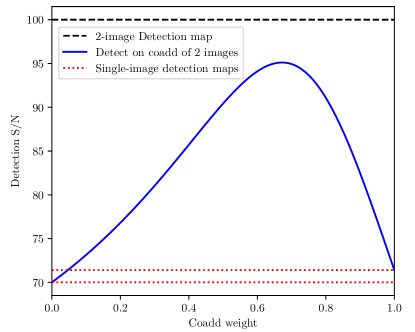
As an illustration, we simulated two images with similar detection signal-to-noise but Gaussian PSFs that differed by a factor of two. We computed the detection map, and also created a series of coadds (trying different weights for the two images), computing the detection map for each, using the correct coadded PSF. As shown in Figure 1, regardless of the coadd weight chosen, detecting on the coadd results in a loss of efficiency compared to the detection map.

4.3 Different bandpass filters: the SED-matched filter

Everything we have said up to now has been based on facts about statistical distributions and should be uncontroversial. In this section we propose a method that is, to our knowledge, new to astronomy, though it flows naturally from the multi-image matched filtering we have discussed. While it is fully defensible, it involves priors so we expect will be slightly controversial. We argue that other proposed methods presume stronger and usually unstated priors.

As we saw in the single-bandpass case, we can combine multiple individual exposures into an aggregate estimate of the flux of a point source. In order to do this, it was essential to calibrate the images so that each one was an estimate of the same underlying quantity. The multiple-bandpass case is similar: For each bandpass, we first combine the images taken in that bandpass into an aggregate estimate. Then, to combine the bandpasses we must scale them so that they are estimates of the same quantity. This requires knowing the spectral energy distribution, or at least the colors in the filters of interest, of the source to be detected; this allows us to scale the various bandpasses so that they are estimates of a common quantity: perhaps the flux in a canonical band, or some other linear quantity such as the integrated intensity.

The intuition here is that if we know that our sources of interest are twice as bright in bandpass A as in bandpass B, then we can convert an estimate of the brightness in band B into an estimate of the brightness in band A by multiplying by two. The variance of the scaled estimate increases appropriately (by a factor of four), so a bandpass in which a source is expected to be faint will contribute an estimate with a large variance and will be downweighted when the estimates are combined. We can also view the problem as one of estimating a total flux that has been split into the different bandpasses, and in that view the SED-matched filter is analogous to the way flux is spread into pixels by the point-spread function (and re-collected by correlating with the matched filter).

Assume we have computed detection maps $D_{j}$, with per-pixel standard deviation $\sigma_{D_{j}}$, for a number of different bandpasses. Assume each bandpass has a known conversion factor $s_{j}$ to the canonical band; that is,

$$D_{j} \sim \mathcal{N}\!\left(Fs_{j}\,,\,\sigma_{D_{j}}^{2}\right)$$ (10)

for flux $F$ in the canonical band. Given a number of such detection maps, we first scale them so they are all estimates of the same quantity, by dividing by $s_{j}$:

$$F_{j} = \frac{D_{j}}{s_{j}}$$ (11)

$$F_{j} \sim \mathcal{N}\!\left(\frac{D_{j}}{s_{j}}\,,\,\frac{\sigma_{D_{j}}^{2}}{s_{j}^{2}}\right)$$ (12)

and assuming that the images are independent, we combine them by inverse-variance weighting to produce the maximum-likelihood estimate for $F$:

$$\hat{F} = \frac{\displaystyle\sum_{j}\frac{D_{j}}{s_{j}}\,\frac{s_{j}^{2}}{\sigma_{D_{j}}^{2}}}{\displaystyle\sum_{j}\frac{s_{j}^{2}}{\sigma_{D_{j}}^{2}}}=\frac{\displaystyle\sum_{j}D_{j}\,s_{j}\,\sigma_{D_{j}}^{-2}}{\displaystyle\sum_{j}s_{j}^{2}\,\sigma_{D_{j}}^{-2}}$$ (13)

with per-pixel error

$$\hat{\sigma}_{F} = \left(\sum_{j}s_{j}^{2}\sigma_{D_{j}}^{-2}\right)^{-\frac{1}{2}}\quad.$$ (14)

For example, if we treat $r$ band as the canonical band and our objects of interest have color $r-i=1$, then we expect the flux in $i$ to be a factor of $2.5$ greater than the flux in $r$; $s_{i}=2.5$, and we will scale our $i$-band detection map $D_{i}$ by $1/s_{i}=0.4$ to produce a prediction for the $r$-band flux. Since the sources are expected to be brighter in $i$ band, we must scale down the $i$-band estimate to produce an $r$-band estimate. The $i$-band variance is also reduced in a corresponding way, so this does not dilute the weight of high-precision measurements.

In practice, for those unwilling to use the Bayesian method presented below, we would advocate computing SED-matched detection maps for a set of spectral energy distributions that sparsely sample the space of sources of interest, and take the union of sources detected. By performing multiple significance tests, more false positives will be generated, so it will be necessary to slightly increasing the detection threshold to maintain false positives at an acceptable level. Since we effectively extract more of the available signal-to-noise by weighting the bands appropriately, our method should still achieve superior completeness at a given purity.

More broadly, we argue that source detection should be used as in initial seed of the likely positions of sources, but that only after inference of the proposed source’s properties using the individual images should one decide whether the source should be kept. This leads toward using slightly lower detection thresholds (that will produce more false positives due to noise), plus additional thresholding after fitting to determine which sources should be kept.

4.4 Comments

Chi-squared coadd.

Szalay et al. (1999) present the idea of using the $\chi^{2}$ statistic of a set of images taken through different bandpass filters. That is, they take pixel-aligned and possibly PSF-filtered images (here we will use detection maps) and compute $\chi^{2}$ pixelwise over bands $j$,

$$\chi^{2} = \sum_{j}\frac{D_{j}^{2}}{\sigma_{D_{j}}^{2}}$$ (15)

and a sufficiently large set of connected pixels with $\chi^{2}$ above a detection threshold is taken as evidence as a source. See Figure 2.

Figure 2: SED-matched versus “chi-squared” detection filters. The data points are (chi-squared) detections above $4.5\sigma$ in one $g$-band and one $r$-band image taken with the Dark Energy Camera, plotted in signal-to-noise space. Points that are not detected in deeper data are marked as “False”; these are mostly clustered around zero (due to noise), with some scattered points near the axes due to single-band artifacts such as cosmic rays. The main locus of “Real” peaks correspond to real stars and galaxies with typical colors. The Chi-squared detection method selects all sources outside the circle (including, in the naive formulation, sources with negative flux in both bands). A single-band detection filter selects all sources above a vertical or horizontal detection threshold. Our “Red” SED-matched filter selects sources where the fluxes in the two bands are consistent with a red SED (in this case, a $g-r$ color of 1). Note that the threshold line is roughly orthogonal to the line between the false positives and the true positives; it separates them efficiently. We have shown the chi-squared detection filter with a threshold of $(5\sigma)^{2}$, which yields a higher false positive rate than a $5\sigma$ threshold in a single-band or SED-match filter.

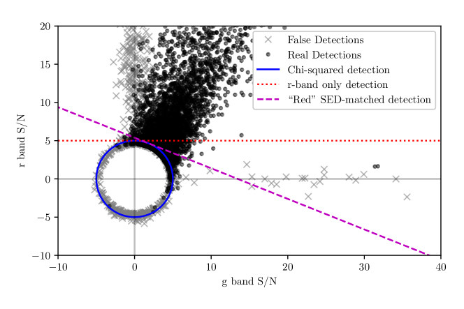
As Szalay et al. (1999) state, the $\chi^{2}$ detection method represents the probability that a pixel is drawn from the Gaussian sky background distribution (independently in each band). A large value is considered to reject this null hypothesis. The “source” hypothesis is not stated, but implicitly, by choosing a constant $\chi^{2}$ threshold, a source is assumed to have any non-zero flux uniformly distributed on the surface of the signal-to-noise (hyper-)sphere. As noted in the paper, this includes sources with negative fluxes in every band. While they suggest heuristics to trim such sources (for example, demanding $>-1\sigma$ of flux in each band), the fact that these sources are detected in the first place hints at the primary issue with this method: that the “source” hypothesis is not physical.

Lacking a source model means that it is not always helpful to add more data: Consider the case where we have one informative band and several noisy (but still somewhat informative) bands. The chi-squared method treats all bands equally, thus mixes the one informative band with all the uninformative bands. When using multiple bands, the detection threshold must be increased to maintain a constant false detection rate (as detailed below), and therefore the number of true detected sources will be lower.

As shown in Figure 2, there is one additional caveat for the chi-squared detection method: a $(5\sigma)^{2}$ threshold yields a larger false positive rate than a standard single-band detection filter with a threshold of $5\sigma$; in order to achieve a desired false positive rate, the detection threshold must be set by analysis (with two bands, the survival function of the chi distribution at the equivalent of $5\sigma$ for a Gaussian is roughly 5.5; with three bands it is roughly 5.75) or simulations (as suggested by Szalay et al. (1999)).

Szalay et al. (1999) in fact also suggest a method for detecting objects of a specific color that is similar but not identical to the approach we present here; they suggest projecting the multiple bands into subspaces and using their chi-squared approach in those subspaces, which means that the issues identified above still hold.

4.5 Going Bayesian

The SED-matched filter presented above tells us how to find likely source positions given a source spectral energy distribution. It is then natural (in a Bayesian framework) to marginalize over the SED using a prior distribution. We can also marginalize over the flux of the source, allowing us to compare the hypothesis that a source exists, versus the hypothesis that the observed flux is due to a noise fluctuation.

We can write the likelihood for a single pixel in the set of detection maps $D_{j}$ for bands $j$, given the existence of a source, as

$$p_{S}(\{D_{j}\})=\iint p(\{D_{j}\}|F,s)\,p(F)\,p(s)\,\mathrm{d}F\,\mathrm{d}s$$ (16)

where $F$ is the flux of the source in some canonical band, and $s$ is the SED of the source; here, we have made the strong assumption that the flux and SED priors are independent. We will assume that the SED prior $p(s)$ is represented as a weighted sum of discrete SEDs: a gridding of SED space, for example. We then have

$$p_{S}(\{D_{j}\}) = \sum_{i}w_{i}\int p(\{D_{j}\}|F,s_{i})\,p(F)\,\mathrm{d}F$$ (17)

$$= \sum_{i}w_{i}\int\prod_{j}\mathcal{N}\!\left(D_{j}\,|\,F\cdot s_{i,j},\sigma_{D_{j}}^{2}\right)\,p(F)\,\mathrm{d}F$$ (18)

$$= \sum_{i}w_{i}\left(\prod_{j}\frac{1}{\sqrt{2\pi}\sigma_{D_{j}}^{2}}\right)\int\exp{\left(\sum_{j}\frac{(D_{j}-F\cdot s_{i,j})^{2}}{-2\,\sigma_{D_{j}}^{2}}\right)}\,p(F)\,\mathrm{d}F$$ (19)

where we have written out the indepedent Gaussian likelihoods of the detection maps, and the SEDs are represented as scalings of the canonical flux $F$: for SED $i$, band $j$ is predicted to have flux $F\cdot s_{i,j}$.

We must now specify a prior over the flux to make progress. One option that leads to a closed-form result is an exponential prior, $p(F)=\alpha\exp(-\alpha F)$ and $F>0$, with $\alpha$ a free variable (to be chosen). We caution that this prior does have some undesirable properties, discussed below. With this exponential flux prior, we have

$$p_{S}(\{D_{j}\}) = K\alpha\sum_{i}w_{i}\int\exp{\left(F\sum_{j}\frac{D_{j}s_{i,j}}{\sigma_{D_{j}}^{2}}\right)}\exp{\left(-F\alpha\right)}\exp{\left(F^{2}\sum_{j}\frac{s_{i,j}^{2}}{\sigma_{D_{j}}^{2}}\right)}\,\mathrm{d}F$$ (20)

where we have pulled out the constant

$$K = \prod_{j}\frac{1}{\sqrt{2\pi}\sigma_{D_{j}}^{2}}\exp{\left(\sum_{j}-\frac{D_{j}^{2}}{2\sigma_{D_{j}}^{2}}\right)}=\mathcal{N}\!\left(D_{j}\,|\,0,\sigma_{D_{j}}^{2}\right)$$ (21)

which will be recognized as the zero-mean Gaussian probability of $\{D_{j}\}$: the likelihood that data values $D_{j}$ are drawn from the background distribution!

Defining variables

$$a_{i} = \alpha-\sum_{j}\frac{D_{j}s_{i,j}}{\sigma_{D_{j}}^{2}}$$ (22)

$$b_{i} = \frac{1}{2}\sum_{j}\frac{s_{i,j}^{2}}{\sigma_{D_{j}}^{2}}$$ (23)

we get an integral in which the flux prior can be integrated analytically:

$$p_{S}(\{D_{j}\}) = K\alpha\sum_{i}w_{i}\int_{0}^{\infty}\exp(-a_{i}F)\exp(-b_{i}F^{2})\,\mathrm{d}F$$ (24)

$$p_{S}(\{D_{j}\}) = K\alpha\sum_{i}w_{i}\frac{\sqrt{\pi}}{2\sqrt{b_{i}}}\exp\left(\frac{a_{i}^{2}}{4b_{i}}\right)\left(1-\textrm{erf}\left(\frac{a_{i}}{2\sqrt{b_{i}}}\right)\right)$$ (25)

which can be evaluated numerically with modest computational cost as long as the number of SEDs $i$ is not too large. In practice, a coarse gridding of SED space yields good results, as shown below.

In order to select sources, we can compare this likelihood to the null-hypothesis likelihood: that there is no source and the observed values are due to noise. Conveniently, the null-hypothesis likelihood is exactly the factor $K$ in the above expression! Determining the threshold at which to accept a peak in the $p_{S}/K$ map as a source can be framed as a Bayesian decision theory problem, or can be tuned on simulations to yield an acceptable false positive rate.

Figure 3: Bayesian SED-matched source detection with a single-SED prior, for illustration. The foreground model is that sources have fluxes that lie along a “Red” SED with color $g-r=1$. Left: Probability contours for the foreground model are inclined in the direction of the prior. The flux prior prefers small fluxes, but has some probability mass extended toward larger fluxes. The background model (null hypothesis) is that there is no source, only noise; these contours are circles centered on zero. The probability contours are spaced in powers of 10. Right: Probability ratio contours for the foreground divided by background model. When performing source detection, these lines mark decision boundaries; points above and to the right of a decision boundary are considered to be detected. The contours are spaced in powers of 10.

Figure 4: Bayesian SED-matched source detection with a three-SED prior. The prior is that astronomical sources are a mixture of $49\%$ “Red” (color $g-r=1$ mag), $49\%$ “Flat” (color $g-r=0$ mag), and $2\%$ $r$-band only ($g$ flux is zero). Left: Probability contours for the foreground model are extended in the directions of the three components of the prior. The background model (null hypothesis) is that there is no source, only noise; these contours are circles centered on zero. The probability contours are spaced in powers of 10. Right: Probability ratio contours for the foreground divided by background model. When performing source detection, these lines mark decision boundaries; points above and to the right of a decision boundary are considered to be detected. The contours are spaced in powers of 10.

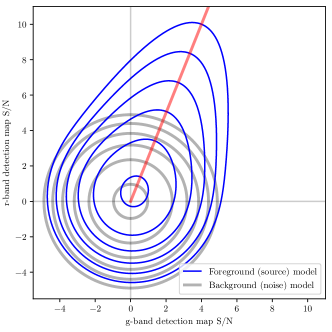
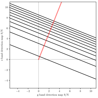
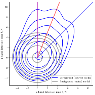
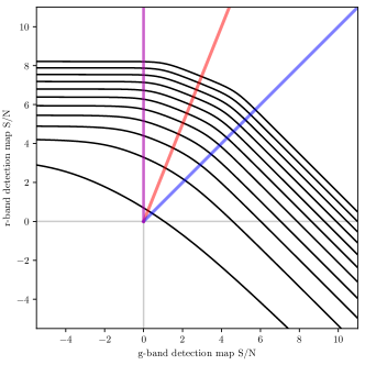
To illustrate the method, we consider a case where we have two bands of imaging, $g$ and $r$ bands. In Figure 3, we plot the probability contours of the background model (equation 21) and the foreground model (equation 25), for the simplest case where our SED prior $p(s)$ is a delta function at $s_{g}=\frac{1}{3.5}$, $s_{r}=\frac{2.5}{3.5}$: this is a “Red” detection filter that assumes a $g-r$ color of 1 magnitude. As expected, the probability contours of the foreground model shift away from negative fluxes and toward fluxes that are consistent with the expected color. The exponential prior on flux causes the foreground model to prefer sources with small fluxes, and therefore the probability mass of the foreground model is clustered around zero. The probability ratio contours—which are what would be used to accept or reject a proposed source—are, as expected, orthogonal to the expected SED vector.

In Figure 4, we show probability contours for a three-SED model, including the “Red” SED and a “Flat” SED ($r$ flux equals $g$ flux) with equal weights of $0.49$, plus an SED that has only flux in the $r$ band, with weight $0.02$. The probability contours of this model are, as before, extended in the directions of these SEDs. The probability ratio contours transition smoothly between being orthogonal to these three SED directions.

Figure 5: The effect of the flux prior in Bayesian SED-matched source detection. In order to produce closed-form integrals, we use an exponential prior on the flux; here we show the effect of the exponential scale factor ($\alpha$) on the results. Left: Probability contours for the “Red” foreground model, as before, and with a flux prior that prefers brighter sources—larger observed fluxes are considered more probable. Right: A one-dimensional example showing the effect of changing the flux prior by a factor of two. The dashed model places more prior belief in larger fluxes, and therefore must produce smaller probabilites at low flux levels. This illustrates that care must be taken with the scale factor of the flux prior.

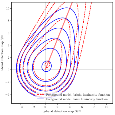
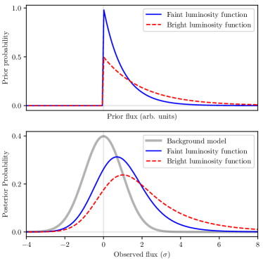
As mentioned previously, there is an issue with the flux prior we are using: it is not scale-free, or rather, it is degenerate with the choice of $\alpha$. That is, the posterior probability is sensitive to the numerical values for the quantity $F$, the “canonical flux”, which we have marginalized out of the expression. We did not put any restrictions on the SED values $s_{i,j}$; we only stated that the predicted flux in band $j$ is given by $F\cdot s_{i,j}$. If we were to scale up all our $s_{i,j}$ values, this would imply a decrease in $F$, which would have higher prior probability, leading to larger posterior probability values. This problem is illustrated in Figure 5. This is obviously undesirable, but thus far we have not been able to find a scale-free prior that leads to tractable integrals.

5 Experiments

We present experiments using data from the Dark Energy Camera (Flaugher et al., 2015) taken as part of the Supernova program (Bernstein et al., 2012) of the Dark Energy Survey (The Dark Energy Survey Collaboration, 2005). We selected the deep field “SN X3” near RA,Dec $=(36.45,-4.6)$, which has a large number of exposures in bands $g$, $r$, $i$ and $z$. For these experiments, we use data from bands $g$, $r$ and $i$ only. We select a set of 25 exposures in each band from the 2016B semester, keeping at most one exposure per night per band. The exposure times for each image are 200 seconds in $g$, 400 seconds in $r$, and 360 seconds in $i$. The images have a range of seeing and sky transparency values. The list of exposures is available in Tables 1 and 2.

Tiny zoom-in	Whole sample

Figure 6: Left: A $600\times 600$-pixel zoom-in of a tiny fraction of the DECam data used in this experiment, coadded and shown with an RGB color scheme and arcsinh stretch. Detected sources are marked with symbols indicating which of the SED-matched filters yields the strongest detection; for clarity here we are using an extremely high detection threshold of $30\sigma$. Right: The positions in color-space of detected sources, classified by the SED-matched filter that yields the strongest detection. The bold circles mark the color to which each filter is tuned. Each SED-matched filter most strongly detects sources nearby in color spaces, where the exact dividing line depends on the signal-to-noise in the different filters.

Blue-optimized	Yellow-optimized	Red-optimized

Figure 7: Source that are most strongly detected by each SED-matched filter. Left: “Blue” SED (matched to color $g-r=r-i=0$). Center: “Yellow” SED (matched to $g-r=1$, $r-i=0.3$). Right: “Red” SED (matched to $g-r=1.5$, $r-i=1$).

Figure 8: Sources that are detected most strongly in one of the single-band SED filters (top row: $g$-band-only; next three rows: $r$-band-only; bottom two rows, $i$-band-only). These sources include asteroids (here, 12 observations of 6 known asteroids, some visibly elongated during these minutes-long exposures), cosmic rays that are not masked by the Community Pipeline, and, for $i$-band-only, some extremely red sources.

Figure 9: Relative strengths of the different SED-matched detection filters. We match our detected sources with the Dark Energy Survey DR1 source database in order to show an accurately measured color for each source. We plot the detection strength (sensitivity) of the “Blue” and “Red” SED-matched filters versus the “Yellow” filter. That is, a source with relative strength 1.1 in the “Blue” filter would be detected at $5.5\sigma$ in the “Blue” filter if it were detected at $5\sigma$ in the “Yellow” filter. As expected, sources with blue $g-i$ colors are most sensitively detected by the “Blue” SED-matched filter, sources with intermediate colors are most sensitively detected by the “Yellow” filter, and red sources are most sensitively detected by the “Red” SED-matched filter. The $g-i$ colors to which the detections filters are matched are marked with vertical lines. Note that the relative sensitivities can be tens of percent, which is very significant at low signal-to-noise levels. The filters are roughly equal at the mid-point between the colors for which they are tuned.

Figure 10: Empirical Bayesian prior for SED-matched detection. Left: Sources from the Dark Energy Survey catalog, in color space. Center: Sources binned in SED space, with low-population bins dropped. The axes are the fraction of flux contributed by the $g$ and $r$ bands, respectively. Implicitly, the fraction contributed by the $i$ band is 1 - ($g$ + $r$). Empty bins are shown with a light shading. Notice that some bins with $g\sim 0$ are populated; these correspond to DES catalog entries with measured $g$ flux consistent with zero. Right: Our discrete SED-space binning, projected to color space.

Figure 11: Bayesian SED-matched detection method compared to the union of $g$, $r$, and $i$ single-band detection. The color-space locations of sources that are detected by both methods are shown as faint points, and sources that are detected by only one method or the other are highlighted. In this experiment, the detection thresholds were tuned so that both methods produced the same number of detections; this compares each method’s best detections. The Bayesian-only detections have the colors of real objects, while the $gri$-union detections tend to be single-band sources, including cosmic rays, asteroids, and very red sources. Cutouts of these sources are shown in Figure 12.

Detected by Bayesian only	Detected by $gri$-union only

Figure 12: Bayesian SED-matched detection method compared to the union of $g$, $r$, and $i$ single-band detections, where each method is allowed to detect the same total number of sources. Left: Examples of sources that are detected by only the Bayesian SED-matched detection method. These have the colors of real objects and appear to be all faint galaxies. Right: Examples of sources that are detected by only the $gri$-union method. These include cosmic rays, asteroids, and very red sources.

Figure 13: Galaxy detection. Left: Detections from an extended-source detector, sorted by the difference in detection strength between the “yellow galaxy” and “yellow point source” detectors. The bright stars are likely included because their saturated cores cause difficulty in correctly measuring the signal-to-noise. The remaining sources are all galaxies, except for one fast-moving asteroid that is spatially extended. Right: Relative strength of detection of sources in the extended versus PSF detection filters. The extended-source filter used here is a 1-arcsecond FWHM round Gaussian. There is a clear line of sources with a detection ratio around 0.95, corresponding to point sources. Sources with ratios above unity are closer in profile to the target profile than to a point source, with the largest ratios probably corresponding to sources that are approximately equal to the target profile.

We use the standard NOAO DECam Community Pipeline (Valdes et al., 2014) for calibration of the images, and then compute astrometric and photometric zeropoints, sky background models and PSF models, using the DESI Legacy Surveys pipeline (Dey et al., 2019), legacypipe. The astrometric calibration uses Gaia (DR1) as the reference catalog (Gaia Collaboration et al., 2016b, a), and the photometric calibration uses the Pan-STARRS DR1 reference catalog (Chambers et al., 2016). The PSF models use PsfEx (Bertin, 2011).

5.1 SED-matched detection

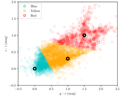
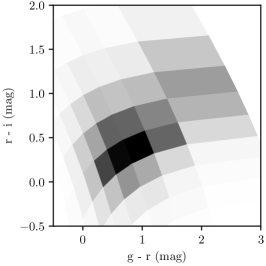
We select a 4000-by-4400 pixel region, at the approximate DECam pixel scale of $0.262$ arcsec/pixel, covering DECam chips N4 and S4 in the center of the focal plane. We produce detection maps for each band as described above, and run several SED-matched filters: a “Blue” filter matched to a source with colors $g-r=r-i=0$; a “Yellow” filter matched to $g-r=1$, $r-i=0.3$; and a “Red” filter matched to $g-r=1.5$, $r-i=1$.

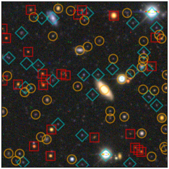
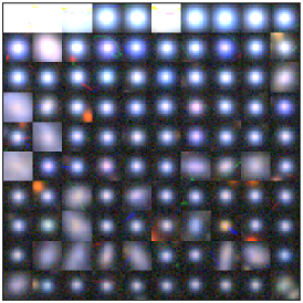
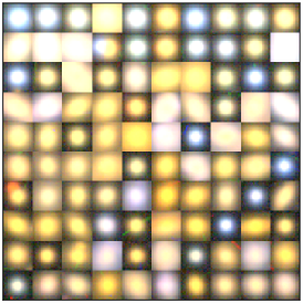
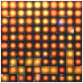
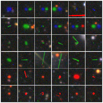
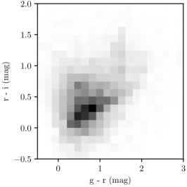
For the plots shows here, we select sources in the Yellow filter with signal-to-noise above $100$, taking as a source the peak pixel within each connected component of pixels above the threshold; we do not try to resolve or deblend nearby peaks. We drop any source near the edge of the image or where there are fewer than 12 exposures in any of $g$, $r$, or $i$ bands. This results in $2092$ detected sources. For each source position, we sample the Red and Blue SED-matched maps so that we can compare the relative sensitivities of the different SED-matched filters. We also sample the detection maps in each band at the peak pixel as an approximate estimate of the flux of the source. This assumes all sources are point sources, so underestimates total flux of galaxies. An image of the detected sources, and the locations in color space of sources that are detected by each SED-matched filter are shown in Figure 6. Figure 7 shows a sample of sources that are most strongly detected by each of the SED-matched filters.

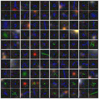
We also observe that some sources are most strongly detected in one of the single-band-only SED-matched filters. For the $g$-band-only and $r$-band-only filters, these are almost exclusively image artifacts, such as cosmic rays that are not masked by the Community Pipeline; and transient sources, including asteroids. The $i$-band-only filter can also detect extremely red sources. A few examples are shown in Figure 8.

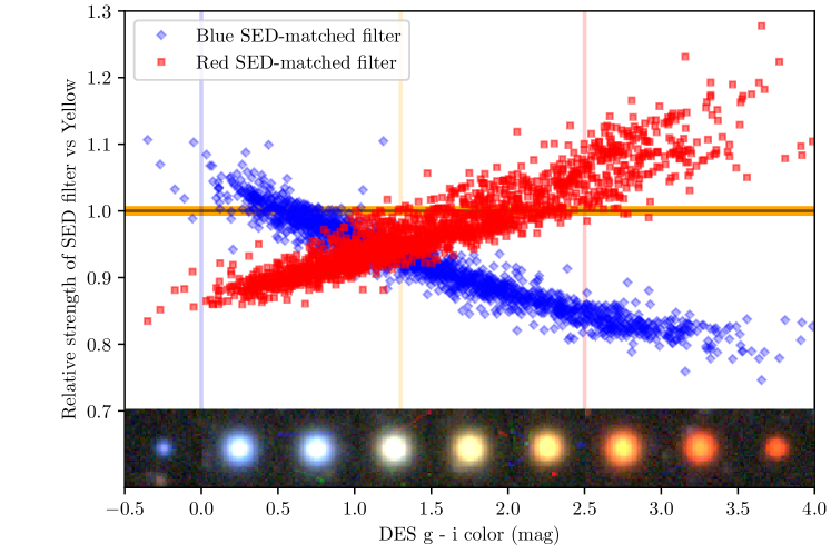
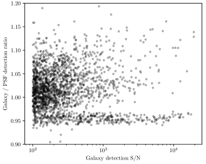
In Figure 9 we illustrate how the relative strength of the different SED-matched filters change with respect to measured source colors. We observe differences of tens of percent, which can lead to a very significant number of additional correctly detected sources at the lowest signal-to-noise levels.

5.2 Bayesian SED-matched detection

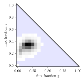
We build an empirical “library” of SEDs for these bands, which we use as a prior, by querying the Dark Energy Survey database in our region of interest. We convert the mag_auto measurements into fluxes, compute the fraction of flux contributed by the $g$, $r$, and $i$ bands, and histogram these values into a $21\times 21$ grid. Keeping bins containing more than $0.1\%$ of the catalog entries, we find 63 bins populated, as shown in Figure 10. The prior includes some SED components that have zero flux in $g$ band, which correspond to very red sources.

We run the Bayesian detection proceduce described in Equation 25, computing in log space to avoid numerical overflow. This takes a few minutes on a single core with our unoptimized implementation.

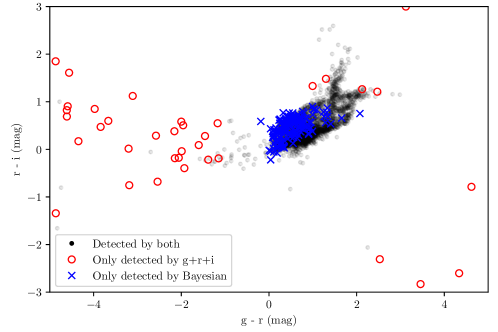
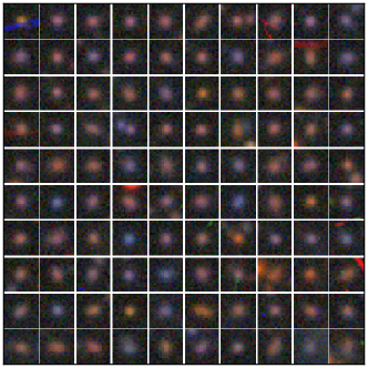
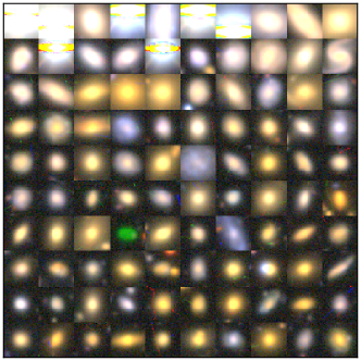
In order to show the performance of the Bayesian approach, we will detect sources at a high threshold and compare against a simple approach. For the Bayesian map, we threshold at a log-probability ratio of $2000$, which yields approximately 3055 sources in good regions of the image. For a comparison, we run the same detection procedure first on our $g$-band map, then on the $r$-band map, and finally on the $i$-band map, with a detection threshold of $50\sigma$ for each band, and keeping the union of all detections. We merge detected sources if they are within 5 pixels of each other. This yields a total of 3201 sources in good regions. In order to find sources that are detected by one method and not the other, we first cut to the brightest 3055 $gri$-union detections (based on maximum signal-to-noise in the three bands) so that the two lists of sources are the same length. We then find sources that are not within an above-threshold region in the other map. That is, we ignore Bayesian detections where the maximum of $g$, $r$, or $i$ signal-to-noise is above $50$, and we drop $gri$-union detections where the Bayesian log-probability is above $2000$. This yields 163 unique Bayesian detections and 112 unique $gri$-union detections. As shown in Figures 11 and 12, the sources detected by only the Bayesian method have the colors of real sources and appear to be all real galaxies, while the sources detected by only the $gri$-union method include a large number of cosmic rays and asteroids, as well as a number of real very red sources. If we clip outlier pixels while forming the detection maps, we can eliminate these cosmic rays before the detection step; the $gri$-union method then preferentially detects sources with extreme colors. Since real images will often contain artifacts and moving objects, the fact that the $gri$-union method prefers these objects to real sources is problematic; the Bayesian method, on the other hand, requires sources with such unexpected colors to have much higher signal than it does for real sources.

5.3 Galaxy detection

While we have focused on the detection of point sources in this paper, it is a trivial extension to build a detection filter tuned to a source with a known spatial profile. We need only correlate the detection maps for each band by the spatial profile of the source to be detected, and compute the corresponding change in uncertainty in the detection maps. In this experiment, we assume a simple round Gaussian profile with a FWHM of 1 arcsecond. After computing extended-source detection maps for each of the $g$, $r$, and $i$ image sets, as above, we run the Yellow SED-matched filter and detect sources as before. In Figure 13 we show sources that are more strongly detected by our extended-source detector than by a point-source detector. These include a few bright stars (where the saturated cores cause errors in estimating the signal-to-noise) but are largely real galaxies. Perhaps surprisingly, we find that using a detection filter tuned to a round Gaussian profile yields only a few-percent improvement in detection efficiency versus a PSF-tuned filter, for typical galaxies in DECam images.

6 Conclusions

We have reviewed the ubiquitous matched filter and shown how it can be used to detect point sources in collections of astronomical images. Our new contribution is to extend the matched filter to SED space in order to combine images taken through multiple bandpass filters. This is a natural extension, but requires specifying the color of the sources to be detected most sensitively. A Bayesian extension of this idea allows us to marginalize over the colors of the sources to be detected, ideally driven by theoretical or empirical models of the sources to be detected. The Bayesian formulation also requires specifying a prior over the fluxes of sources. We present an exponential prior that leads to a closed-form expression for the fully marginalized Bayesian detection probability; this can be computed inexpensively.

A pleasing aspect of the matched-filtering approach—including our extension to SED-matched filtering—is that it can correctly use all available data. Images that are known a priori to contribute little information due to their noise levels or because the source is known to have small flux in that band, are downweighted but not ignored entirely. This property will becomes increasingly useful as multi-wavelength, many-exposure, multi-instrument studies become more prominent.

Appendix A Deriving the matched filter

Let us assume that there exists a linear filter whose output allows optimal detection of isolated point sources. That is, we seek a (two-dimensional) set of coefficients $a_{\boldsymbol{i}}$ that, when correlated with the image $I_{\boldsymbol{j}}$, produces a map $M_{\boldsymbol{j}}$ whose peak is the likely location of the point source.

The linear filtering (correlation) operation is

$$M_{\boldsymbol{j}}=\sum_{\boldsymbol{i}\,\,\mathrm{in}\,\,\mathcal{A}}a_{\boldsymbol{i}}\,I_{\boldsymbol{i}+\boldsymbol{j}}$$ (A1)

where $\mathcal{A}$ is the support of $\boldsymbol{a}$ (integer pixel positions), and the center of $\boldsymbol{a}$ is $(0,0)$. We will demand that the elements of $\boldsymbol{a}$ are non-negative and sum to unity.

Inserting equation 1, we get

$$M_{\boldsymbol{j}} \sim \sum_{\boldsymbol{i}\,\,\mathrm{in}\,\,\mathcal{A}}I_{k}\,a_{\boldsymbol{i}}\,\psi_{\boldsymbol{i}+\boldsymbol{j}-\boldsymbol{k}}+\mathcal{N}\!\left(0\,,\,\sigma_{1}^{2}\right)$$ (A2)

$$\sim \mathcal{N}\!\left(I_{k}\sum_{\boldsymbol{i}\,\,\mathrm{in}\,\,\mathcal{A}}a_{\boldsymbol{i}}\,\psi_{\boldsymbol{i}+\boldsymbol{j}-\boldsymbol{k}}\,,\,\sum_{\boldsymbol{i}\,\,\mathrm{in}\,\,\mathcal{A}}a_{\boldsymbol{i}}^{2}\,\sigma_{1}^{2}\right)$$ (A3)

and the per-pixel signal-to-noise in the map is

$$\mathbb{SN}(M_{\boldsymbol{j}})=\frac{I_{k}\,\sum a_{\boldsymbol{i}}\,\psi_{\boldsymbol{i}+\boldsymbol{j}-\boldsymbol{k}}}{\sigma_{1}\sqrt{\sum_{\boldsymbol{i}}a_{\boldsymbol{i}}^{2}}}\quad.$$ (A4)

We want to choose coefficients $a_{\boldsymbol{i}}$ to maximize the signal-to-noise at the true pixel position of the source, $\boldsymbol{k}$. Rewriting the expression using dot-products and ($\ell_{2}$) norms, treating the two-dimensional images $a_{\boldsymbol{i}}$ and $\psi_{\boldsymbol{i}+\boldsymbol{j}-\boldsymbol{k}}$ as vectors indexed by $\boldsymbol{i}$, we have:

$$\mathbb{SN}(M_{\boldsymbol{j}}) = \frac{I_{k}\,\boldsymbol{a}\cdot\bm{\psi_{j-k}}}{\sigma_{1}\sqrt{\boldsymbol{a}\cdot\boldsymbol{a}}}$$ (A5)

$$= \frac{I_{k}\,\left\lVert\boldsymbol{a}\right\rVert\left\lVert\bm{\psi_{j-k}}\right\rVert\cos\theta}{\sigma_{1}\left\lVert\boldsymbol{a}\right\rVert}$$ (A6)

$$= \frac{I_{k}\,\left\lVert\bm{\psi_{j-k}}\right\rVert\cos\theta}{\sigma_{1}}$$ (A7)

where $\theta$ is a generalized angle between $\boldsymbol{a}$ and $\bm{\psi_{j-k}}$. At the pixel position of the source, $\boldsymbol{k}$,

$$\mathbb{SN}(M_{\boldsymbol{k}})=\frac{I_{k}\,\left\lVert\bm{\psi_{0}}\right\rVert\cos\theta}{\sigma_{1}}$$ (A8)

Clearly this is maximized when $\theta=0$, i.e., when $\boldsymbol{a}$ is a multiple of $\bm{\psi_{0}}$, the PSF evaluated at a grid of integer pixel positions. Since we have defined both the PSF and coefficients $a$ to sum to unity, we find that the optimal linear filter for detection is given by:

$$\boldsymbol{a}=\bm{\psi_{0}}\quad,$$ (A9)

which means that the operation of correlating the image with its PSF produces a map with optimal signal-to-noise. Repeating equation A1, we have found that the map $M_{\boldsymbol{j}}$ can be computed by correlating the image with its PSF:

$$M_{\boldsymbol{j}}=\sum_{\boldsymbol{i}\,\,\mathrm{in}\,\,\mathcal{A}}\psi_{\boldsymbol{i}}\,I_{\boldsymbol{i}+\boldsymbol{j}}\quad,$$ (A10)

where, as before, $\mathcal{A}$ is the support of the PSF.

The signal-to-noise in this map at the true source pixel position $\boldsymbol{k}$ is

$$\mathbb{SN}(M_{\boldsymbol{k}})=\frac{I_{k}\,\left\lVert\bm{\psi}\right\rVert}{\sigma_{1}}\quad.$$ (A11)

A.1 Optimality

We compute the variance of the detection map estimator (equation 2), and show that is equal to the Cramér–Rao bound. Substituting our image model into the detection map,

$$D_{\boldsymbol{j}} = \frac{1}{\left\lVert\bm{\psi}\right\rVert^{2}}\sum_{i}\psi_{\boldsymbol{i}}\,I_{\boldsymbol{i}+\boldsymbol{j}}$$ (A12)

$$\sim \frac{1}{\left\lVert\bm{\psi}\right\rVert^{2}}\sum_{i}\psi_{\boldsymbol{i}}\,\mathcal{N}\!\left(F\,\psi_{\boldsymbol{i}+\boldsymbol{j}-\boldsymbol{k}}\,,\,\sigma_{1}^{2}\right)$$ (A13)

and at the true source position, $\boldsymbol{j}=\boldsymbol{k}$;

$$D_{\boldsymbol{k}} \sim \frac{1}{\left\lVert\bm{\psi}\right\rVert^{2}}\mathcal{N}\!\left(F\,\sum_{i}\psi_{\boldsymbol{i}}^{2}\,,\,\sum_{i}\psi_{\boldsymbol{i}}^{2}\sigma_{1}^{2}\right)$$ (A14)

$$D_{\boldsymbol{k}} \sim \mathcal{N}\!\left(F\,,\,\frac{\sigma_{1}^{2}}{\left\lVert\bm{\psi}\right\rVert^{2}}\right)$$ (A15)

so the variance of the estimator is $\mathrm{var}\left(D\right)=\frac{\sigma_{1}^{2}}{\left\lVert\bm{\psi}\right\rVert^{2}}$.

Meanwhile, the Fisher Information for $F$ given pixel values $I_{\boldsymbol{j}}$ is

$$I(F) = -\mathbb{E}_{I_{\boldsymbol{j}}}\left[\frac{\partial^{2}\log P(\{I_{\boldsymbol{j}}\}|F)}{\partial F^{2}}\right]$$ (A16)

and with pixel values $I_{\boldsymbol{j}}$ the likelihood is

$$I_{\boldsymbol{j}} \sim \mathcal{N}\!\left(F\psi_{\boldsymbol{j}}\,,\,\sigma_{1}^{2}\right)$$ (A17)

$$P(\{I_{\boldsymbol{j}}\}|F) = \prod_{\boldsymbol{j}}\frac{1}{\sqrt{2\pi\sigma_{1}^{2}}}\exp\left(-\frac{(I_{\boldsymbol{j}}-F\psi_{\boldsymbol{j}})^{2}}{2\sigma_{1}^{2}}\right)$$ (A18)

$$\frac{\partial^{2}}{\partial F^{2}}\log P(\{I_{\boldsymbol{j}}\}|F) = \sum_{\boldsymbol{j}}-\frac{\psi_{\boldsymbol{j}}^{2}}{\sigma_{1}^{2}}$$ (A19)

which is independent of $I_{\boldsymbol{j}}$, so

$$I(F) = \frac{\left\lVert\psi\right\rVert^{2}}{\sigma_{1}^{2}}$$ (A20)

from which we see that the estimator $D$ saturates the Cramér–Rao bound.

A.2 Norm of a Gaussian PSF

For a Gaussian PSF with standard deviation $w$ pixels,

$$\displaystyle\psi^{G}(x,y) = \frac{1}{2\pi w^{2}}\exp{\left(-\frac{x^{2}}{2w^{2}}\right)}\exp{\left(-\frac{y^{2}}{2w^{2}}\right)}$$ (A21)

the norm is

$$\left\lVert\bm{\psi^{G}}\right\rVert = \sqrt{\sum_{x}\sum_{y}\left(\frac{1}{2\pi w^{2}}\exp{\left(-\frac{x^{2}}{2w^{2}}\right)}\exp{\left(-\frac{y^{2}}{2w^{2}}\right)}\right)^{2}}$$ (A22)

$$\left\lVert\bm{\psi^{G}}\right\rVert \simeq \sqrt{\iint\frac{1}{4\pi^{2}w^{4}}\exp{\left(-\frac{x^{2}}{w^{2}}\right)}\exp{\left(-\frac{y^{2}}{w^{2}}\right)}\mathrm{d}x\,\mathrm{d}y}$$ (A23)

$$\left\lVert\bm{\psi^{G}}\right\rVert \simeq \frac{1}{2\sqrt{\pi}w}$$ (A24)

so the detection map has signal-to-noise at the true source position $\boldsymbol{k}$,

$$\mathbb{SN}(D_{\boldsymbol{k}}^{G})=\frac{I_{k}}{2\sqrt{\pi}w\sigma_{1}}\quad.$$ (A25)

Note, however, that we have defined the point-spread function $\psi(\cdot)$ to be the pixel-convolved response, so it cannot be exactly Gaussian if the pixel response is assumed to be a boxcar function. In practice, however, a two-dimensional Gaussian with variance $v^{2}$ correlated with a two-dimensional boxcar function is well approximated by a Gaussian with variance $v^{2}+\frac{1}{12}$, as long as $v\gtrsim\frac{1}{2}$.

A.3 Why not signal-to-noise-squared?

In correlating the image with the PSF, it looks like the detection map weights pixels by their signal-to-noise, rather than signal-to-noise squared. This apparent conflict can be resolved by scaling the pixel values so that each pixel is an estimate of the same quantity. That is, we want to estimate the total source counts $F$, but the pixels contain estimates of the source counts scaled by the PSF, $F\psi$; we must undo this scaling by multiplying the pixels by $1/\psi$.

Given a source at position $\boldsymbol{k}$, we define the image $K$ whose pixels each contain an estimate of the total source counts:

$$K_{\boldsymbol{j}} = \frac{1}{\psi_{\boldsymbol{j}-\boldsymbol{k}}}S_{\boldsymbol{j}}$$ (A26)

$$K_{\boldsymbol{j}} \sim \frac{1}{\psi_{\boldsymbol{j}-\boldsymbol{k}}}\,\mathcal{N}\!\left(I_{k}\,\psi_{\boldsymbol{j}-\boldsymbol{k}}\,,\,\sigma_{1}^{2}\right)$$ (A27)

$$K_{\boldsymbol{j}} \sim \mathcal{N}\!\left(I_{k}\,,\,\frac{\sigma_{1}^{2}}{\psi_{\boldsymbol{j}-\boldsymbol{k}}^{2}}\right)\quad.$$ (A28)

The signal-to-noise remains the same, since we have just scaled the values:

$$\mathbb{SN}(K_{\boldsymbol{j}}) = \frac{I_{k}\,\psi_{\boldsymbol{j}-\boldsymbol{k}}}{\sigma_{1}}$$ (A29)

$$\mathbb{SN}(K_{\boldsymbol{j}}) = \mathbb{SN}(S_{\boldsymbol{j}})\quad.$$ (A30)

As before, the detection map pixels are a linear combination of the (shifted) pixels of the $K$ image with weights $b_{\boldsymbol{i}}$:

$$D_{\boldsymbol{j}}^{\star} = \sum_{\boldsymbol{i}}b_{\boldsymbol{i}}\,K_{\boldsymbol{i}+\boldsymbol{j}}$$ (A31)

$$\sim \sum_{\boldsymbol{i}}b_{\boldsymbol{i}}\,\mathcal{N}\!\left(I_{k}\,,\,\frac{\sigma_{1}^{2}}{\psi_{\boldsymbol{i}+\boldsymbol{j}-\boldsymbol{k}}^{2}}\right)$$ (A32)

$$\sim \mathcal{N}\!\left(I_{k}\sum_{\boldsymbol{i}}b_{\boldsymbol{i}}\,,\,\sum_{\boldsymbol{i}}\frac{b_{\boldsymbol{i}}^{2}\sigma_{1}^{2}}{\psi_{\boldsymbol{i}+\boldsymbol{j}-\boldsymbol{k}}^{2}}\right)$$ (A33)

and the signal-to-noise in that detection map at pixel $\boldsymbol{k}$ is

$$\mathbb{SN}(D_{\boldsymbol{k}}^{\star}) = \frac{I_{k}\sum_{\boldsymbol{i}}b_{\boldsymbol{i}}}{\sigma_{1}\sqrt{\sum_{\boldsymbol{i}}\frac{b_{\boldsymbol{i}}^{2}}{\psi_{\boldsymbol{i}}^{2}}}}$$ (A34)

which is maximized by setting the $b_{\boldsymbol{i}}$

$$b_{\boldsymbol{i}}\propto\psi_{\boldsymbol{i}}^{2}\quad:$$ (A35)

proportional to the signal-to-noise squared, as expected.

Appendix B Multi-image detection

B.1 Optimality

As before, we will show that the estimator $F^{\star}$ in Equation 8 saturates the Cramér–Rao bound for $F$.

We will consider two images, $A$ and $B$, with PSFs $\psi$ and $\phi$, respectively, and calibration factors $\kappa_{A}$ and $\kappa_{B}$ that scale image units to flux units. Per-pixel noise in the two images will be $\sigma_{A}$ and $\sigma_{B}$. We will assume that the pixel grids are aligned so that no resampling is necessary.

Given all this, the pixel value for images $A$ and $B$ are drawn from the distributions

$$A \sim \mathcal{N}\!\left(\frac{F}{\kappa_{A}}\psi_{k}\,,\,\sigma_{A}^{2}\right)$$ (B1)

$$B \sim \mathcal{N}\!\left(\frac{F}{\kappa_{B}}\phi_{k}\,,\,\sigma_{B}^{2}\right)\quad.$$ (B2)

The Fisher Information is

$$I(F) = -\mathbb{E}_{A,B}\left[\frac{\partial^{2}\log P(\{A,B\}|F)}{\partial F^{2}}\right]$$ (B3)

and assuming that images $A$ and $B$ are statistically independent, $P(A,B|F)=P(A|F)P(B|F)$. Following the analysis in A.1, we find that

$$I(F) = \frac{\left\lVert\psi\right\rVert^{2}}{\kappa_{A}^{2}\sigma_{A}^{2}}+\frac{\left\lVert\phi\right\rVert^{2}}{\kappa_{B}^{2}\sigma_{B}^{2}}$$ (B4)

which equals the variance of the $F^{\star}$ estimator, $\sigma_{F^{\star}}^{2}$ as given in Equation 9. Therefore, the estimator saturates the Cramér–Rao bound.

B.2 Experiments

Filter	Exposure number	Date	Exposure time (s)	Seeing (arcsec)	Depth ($5\sigma$ point source)
g	563982	2016-08-14	200	1.28	24.65
g	566968	2016-08-24	200	1.79	23.02
g	567422	2016-08-25	200	1.72	23.55
g	569591	2016-08-31	200	1.55	24.39
g	571049	2016-09-05	200	1.67	24.29
g	573546	2016-09-11	200	1.42	24.49
g	574702	2016-09-14	200	2.17	22.75
g	575794	2016-09-22	200	1.20	24.17
g	577432	2016-09-26	200	1.55	24.47
g	579874	2016-10-02	200	1.37	24.51
g	582140	2016-10-09	200	1.61	23.56
g	584106	2016-10-20	200	1.64	24.05
g	585888	2016-10-25	200	2.00	24.11
g	588620	2016-11-02	200	1.39	24.43
g	591449	2016-11-09	200	1.47	23.53
g	593383	2016-11-17	200	1.53	24.39
g	595093	2016-11-22	200	1.45	24.48
g	596474	2016-11-26	200	1.07	24.80
g	598232	2016-12-01	200	1.96	23.91
g	600846	2016-12-08	200	1.20	23.69
g	601468	2016-12-17	200	1.32	23.41
g	603288	2016-12-22	200	1.55	24.35
g	604684	2016-12-28	200	1.82	24.26
g	605946	2017-01-03	200	1.75	24.11
g	609567	2017-01-17	200	1.17	24.14
r	563978	2016-08-14	400	1.37	24.51
r	566976	2016-08-24	400	1.58	23.57
r	567426	2016-08-25	400	1.53	23.99
r	569613	2016-08-31	400	1.18	24.82
r	571060	2016-09-05	400	1.64	24.51
r	573562	2016-09-11	400	1.34	24.19
r	574711	2016-09-14	400	1.47	23.82
r	575798	2016-09-22	400	1.07	24.33
r	576542	2016-09-24	400	1.67	24.44
r	578740	2016-09-29	400	1.54	24.46
r	580295	2016-10-03	400	1.62	24.34
r	582423	2016-10-10	400	1.07	24.12
r	584144	2016-10-20	400	1.55	23.91
r	585892	2016-10-25	400	1.90	24.15
r	588624	2016-11-02	400	1.25	24.61
r	591453	2016-11-09	400	1.16	24.30
r	593076	2016-11-16	400	1.15	23.52
r	593387	2016-11-17	400	1.35	24.64
r	595359	2016-11-23	400	1.85	24.20
r	597239	2016-11-28	400	1.84	24.33
r	598940	2016-12-03	400	1.43	24.46
r	600880	2016-12-08	400	2.67	23.26
r	601776	2016-12-18	400	1.20	24.98
r	604334	2016-12-25	400	1.01	25.05
r	605255	2016-12-30	400	1.50	24.64

Table 1: Exposures in $g$ and $r$ bands from the Dark Energy Camera used in the experiments.

Filter	Exposure number	Date	Exposure time (s)	Seeing (arcsec)	Depth ($5\sigma$ point source)
i	563972	2016-08-14	360	1.77	23.49
i	566980	2016-08-24	360	1.35	23.61
i	567442	2016-08-25	360	1.05	24.20
i	567867	2016-08-26	360	1.04	24.24
i	570175	2016-09-02	360	1.81	23.10
i	571447	2016-09-06	360	1.54	23.23
i	573865	2016-09-12	360	1.66	23.01
i	574727	2016-09-14	360	1.80	22.73
i	575802	2016-09-22	360	1.09	23.13
i	576546	2016-09-24	360	1.41	23.33
i	579449	2016-10-01	360	1.15	23.41
i	581861	2016-10-08	360	1.47	23.03
i	584166	2016-10-20	360	1.27	23.01
i	585960	2016-10-25	360	1.73	22.89
i	588628	2016-11-02	360	1.20	23.93
i	591457	2016-11-09	360	1.06	24.00
i	593080	2016-11-16	360	1.03	23.51
i	595056	2016-11-22	360	1.81	23.75
i	596517	2016-11-26	360	1.61	24.00
i	598236	2016-12-01	360	1.38	23.88
i	600850	2016-12-08	360	1.04	24.12
i	601780	2016-12-18	360	1.12	24.44
i	604338	2016-12-25	360	1.14	24.23
i	605266	2016-12-30	360	1.67	23.90
i	607844	2017-01-09	360	1.34	22.65

Table 2: Exposures in $i$ band from the Dark Energy Camera used in the experiments.

References

- Abbott et al. (2016) Abbott, B. P., Abbott, R., Abbott, T. D., et al. 2016, Physical Review Letters, 116, 061102
- Bernstein et al. (2012) Bernstein, J. P., Kessler, R., Kuhlmann, S., Biswasal, R., et al. 2012, ApJ, 753, astro-ph/1111.1969
- Bertin (2011) Bertin, E. 2011, in Astronomical Society of the Pacific Conference Series, Vol. 442, Astronomical Data Analysis Software and Systems XX, ed. I. N. Evans, A. Accomazzi, D. J. Mink, & A. H. Rots, 435
- Bolton et al. (2012) Bolton, A. S., Schlegel, D. J., Aubourg, É., et al. 2012, AJ, 144, 144
- Chambers et al. (2016) Chambers, K. C., Magnier, E. A., Metcalfe, N., et al. 2016, ArXiv e-prints, arXiv:1612.05560
- Dey et al. (2019) Dey, A., Schlegel, D. J., Lang, D., et al. 2019, AJ, 157, 168
- Doyle et al. (2000) Doyle, L. R., Deeg, H. J., Kozhevnikov, V. P., et al. 2000, The Astrophysical Journal, 535, 338
- Flaugher et al. (2015) Flaugher, B., Diehl, H. T., Honscheid, K., et al. 2015, AJ, 150, 150
- Gaia Collaboration et al. (2016a) Gaia Collaboration, Brown, A. G. A., Vallenari, A., et al. 2016a, A&A, 595, A2
- Gaia Collaboration et al. (2016b) Gaia Collaboration, Prusti, T., de Bruijne, J. H. J., et al. 2016b, A&A, 595, A1
- Hogg & Lang (2013) Hogg, D. W., & Lang, D. 2013, PASP, 125, 719
- Lang et al. (2016) Lang, D., Hogg, D. W., & Schlegel, D. J. 2016, AJ, 151, 36
- Melin et al. (2006) Melin, J.-B., Bartlett, J. G., & Delabrouille, J. 2006, A&A, 459, 341
- Rykoff et al. (2014) Rykoff, E. S., Rozo, E., Busha, M. T., et al. 2014, ApJ, 785, 104
- Szalay et al. (1999) Szalay, A. S., Connolly, A. J., & Szokoly, G. P. 1999, AJ, 117, 68
- The Dark Energy Survey Collaboration (2005) The Dark Energy Survey Collaboration. 2005, ArXiv Astrophysics e-prints, astro-ph/0510346
- Valdes et al. (2014) Valdes, F., Gruendl, R., & DES Project. 2014, in Astronomical Society of the Pacific Conference Series, Vol. 485, Astronomical Data Analysis Software and Systems XXIII, ed. N. Manset & P. Forshay, 379
- Willman et al. (2005) Willman, B., Blanton, M. R., West, A. A., et al. 2005, AJ, 129, 2692
- Zackay & Ofek (2017) Zackay, B., & Ofek, E. O. 2017, ApJ, 836, 187