Multidimensional Uncertainty-Aware Evidential Neural Networks

Abstract

Traditional deep neural networks (NNs) have significantly contributed to the state-of-the-art performance in the task of classification under various application domains. However, NNs have not considered inherent uncertainty in data associated with the class probabilities where misclassification under uncertainty may easily introduce high risk in decision making in real-world contexts (e.g., misclassification of objects in roads leads to serious accidents). Unlike Bayesian NN that indirectly infer uncertainty through weight uncertainties, evidential NNs (ENNs) have been recently proposed to explicitly model the uncertainty of class probabilities and use them for classification tasks. An ENN offers the formulation of the predictions of NNs as subjective opinions and learns the function by collecting an amount of evidence that can form the subjective opinions by a deterministic NN from data. However, the ENN is trained as a black box without explicitly considering inherent uncertainty in data with their different root causes, such as vacuity (i.e., uncertainty due to a lack of evidence) or dissonance (i.e., uncertainty due to conflicting evidence). By considering the multidimensional uncertainty, we proposed a novel uncertainty-aware evidential NN called WGAN-ENN (WENN) for solving an out-of-distribution (OOD) detection problem. We took a hybrid approach that combines Wasserstein Generative Adversarial Network (WGAN) with ENNs to jointly train a model with prior knowledge of a certain class, which has high vacuity for OOD samples. Via extensive empirical experiments based on both synthetic and real-world datasets, we demonstrated that the estimation of uncertainty by WENN can significantly help distinguish OOD samples from boundary samples. WENN outperformed in OOD detection when compared with other competitive counterparts.

Introduction

Deep Learning (DL) models have recently gained tremendous attention in the data science community. Despite their superior performance in various decision making tasks, inherent uncertainty derived from data based on different root causes has not been sufficiently explored. Predictive uncertainty estimation using Bayesian neural networks (BNNs) has been explored for classification prediction or regression in computer vision applications (Kendall and Gal 2017). They considered well-known uncertainty types, such as aleatoric uncertainty (AU) and epistemic uncertainty (EU), where AU only considers data uncertainty caused by statistical randomness (e.g., observation noises) while EU refers to model uncertainty introduced by limited knowledge or ignorance in collected data. On the other hand, in the belief/evidence theory, Subjective Logic (SL) (Jøsang, Cho, and Chen 2018) considered vacuity, which is caused by a lack of evidence, as the key dimension of uncertainty. In addition to vacuity, they also defined other types of uncertainty, such as dissonance (e.g., uncertainty due to conflicting evidence) or vagueness (e.g., uncertainty due to multiple beliefs on a same observation).

Although conventional deep NNs (DNNs) have been commonly used to solve classification tasks, uncertainty associated with classification classes has been significantly less considered in NNs even if the risk introduced by misclassification may bring disastrous consequence in real-world situations, such as car crash due to the misclassification of objects in roads. Recently, techniques using evidential neural networks (ENNs) (Sensoy, Kaplan, and Kandemir 2018) have been proposed to explicitly model the uncertainty of class probabilities. An ENN uses the predictions of an NN as subjective opinions and learns a function that collects an amount of evidence to form the opinions by a deterministic NN from data. However, the ENN is trained as a black box without explicitly considering different types of uncertainty in the data (e.g., vacuity or dissonance), which often results in overconfidence when tested with out-of-distribution (OOD) samples. We measure the extent of confidence in a given classification decision based on the high class probability of a given class (i.e., a belief in SL). Overconfidence refers to a high class probability in an incorrect class prediction. To mitigate the overconfidence issue, regularization methods have proposed to hand-pick auxiliary OOD samples to train the model (Malinin and Gales 2018; Zhao et al. 2019). However, the regularization methods with prior knowledge require a large amount of OOD samples to ensure the good generalization of a model behaviour to the whole data space.

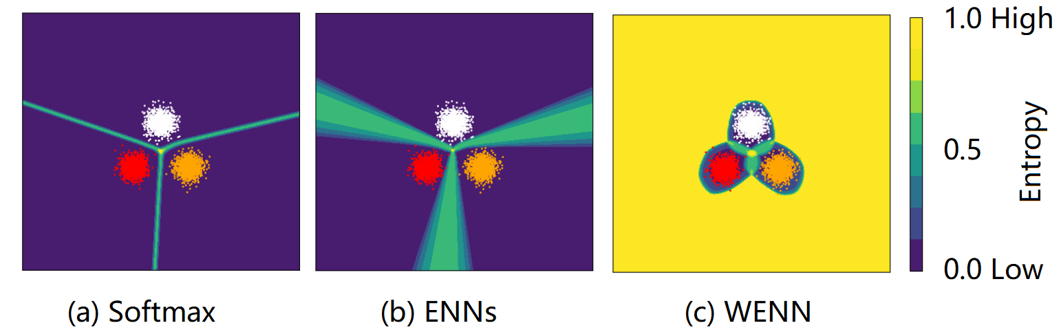
Figure 1: Uncertainty (entropy) estimation based on synthetic data: (a) using standard NNs with softmax function; (b) using ENNs; and (c) using WENN. Only (c) shows high uncertainty in both boundary and OOD regions.

In this work, we propose a model called WGAN-ENN (WENN) that combines ENNs with Wasserstein GAN (WGAN) (Arjovsky, Chintala, and Bottou 2017) to jointly train a model with prior knowledge of a certain class (e.g., high vacuity OOD or high dissonance in-class boundary samples) to reinforce and achieve high prediction confidence only for in-distribution (ID) regions, high vacuity only for OOD samples, and high dissonance only for ID boundary samples.

To briefly demonstrate the performance of uncertainty estimation by conventional NNs, ENNs, and our proposed WENN model, we explain it with a simple three-class classification problem in Fig 1. We measure entropy (Shannon 1948) estimated on the predictive class probabilities by three different approaches: (i) Fig 1 (a) shows the prediction for boundary or OOD samples by traditional NNs (i.e., BNN to indirectly infer uncertainty through weight uncertainties) using the softmax and demonstrates overconfidence; (ii) Fig 1 (b) shows the overconfidence in the prediction of OOD samples by the ENN; and (iii) Fig 1 (c) shows the high confidence in the prediction of the ID region by WENN.

This work provides the following key contributions:

• We considered inherent uncertainties derived from different root causes by taking a hybrid approach that leverages both deep learning and belief model (i.e., Subjective Logic or SL). Although both fields have studied uncertainty-aware approaches to tackle various kinds of decision making problems, there has been lack of efforts to leverage both of their merits. We believe this work sheds light on the direction of incorporating both fields.

• We considered ENNs to quantify multidimensional uncertainty types in data and learn subjective opinions. In particular, the subjective opinions formulated by the SL can be easily leveraged for the quantification of multidimensional uncertainties where we measured vacuity and dissonance based on SL.

• Our proposed WENN, combining WGAN and ENNs, can generate a sufficient amount of auxiliary OOD samples for training and use the Wasserstein distance to measure the variety of those samples. Our proposed alternating algorithm can leverage all the intermediate samples more efficiently than other regularized methods.

• We demonstrated that WENN outperforms competitive state-of-the-art counterparts in OOD detection, showing 7% better performance than the best of the counterparts in the most difficult scenario CIFAR10 vs CIFAR100.

Related Work

Uncertainty Quantification in Bayesian Deep Learning (BDL): Machine/deep learning (ML/DL) researchers considered aleatoric uncertainty (AU) and epistemic uncertainty (EU) based on Bayesian Neural Networks (BNNs) for computer vision applications. AU consists of homoscedastic uncertainty (i.e., constant errors for different inputs) and heteroscedastic uncertainty (i.e., different errors for different inputs) (Gal 2016). A BDL framework was presented to estimate both AU and EU simultaneously in regression settings (e.g., depth regression) and classification settings (e.g., semantic segmentation) (Kendall and Gal 2017). Dropout variational inference (Gal and Ghahramani 2016) was proposed as one of key approximate inference techniques in BNNs  (Blundell et al. 2015; Pawlowski et al. 2017). Later distributional uncertainty is defined based on distributional mismatch between the test and training data distributions (Malinin and Gales 2018).

Uncertainty Quantification in Belief/Evidence Theory: In belief/evidence theory, uncertainty reasoning has been substantially explored in Fuzzy Logic (De Silva 2018), Dempster-Shafer Theory (DST) (Sentz, Ferson et al. 2002), or Subjective Logic (SL) (Jøsang 2016). Unlike the efforts in ML/DL above, belief/evidence theory focused on reasoning of inherent uncertainty in information resulting from unreliable, incomplete, deceptive, and/or conflicting evidence. SL considered uncertainty in subjective opinions in terms of vacuity (i.e., a lack of evidence) and vagueness (i.e., failure of discriminating a belief state) (Jøsang 2016). Recently, other dimensions of uncertainty have been studied, such as dissonance (due to conflicting evidence) and consonance (due to evidence about composite subsets of state values) (Jøsang, Cho, and Chen 2018). In DNNs, (Sensoy, Kaplan, and Kandemir 2018) proposed ENN models to explicitly modeling uncertainty using SL. However, it only considered predictive entropy to qualify uncertainty.

Out-of-Distribution Detection: Recent OOD detection approaches began to use NNs in a supervised fashion that outperformed traditional models, such as kernel density estimation and one-class support vector machine in handling complex datasets (Hendrycks and Gimpel 2016). Many of these models (Liang, Li, and Srikant 2017; Hendrycks, Mazeika, and Dietterich 2018) integrated auxiliary datasets to adjust the estimated scores derived from prediction probabilities. These OOD detection models were specifically designed to detect OOD samples. In addition, well-designed uncertainty estimation models are leveraged for OOD detection. Recently, uncertainty models (Sensoy et al. 2020) have shown their preliminary results on OOD detection by conducting performance comparison of various OOD detection models.

Preliminaries

This section provides the background knowledge to understand this work, including: (1) subjective opinions in SL; (2) uncertainty characteristics of subjective opinion; and (3) ENNs to predict subjective opinions.

Subjective Opinions in SL

A multinomial opinion in a given proposition $x$ is represented by $\omega_{Y}=(\bm{b}_{Y},u_{Y},\bm{a}_{Y})$ where a domain is $\mathbb{Y}\equiv\{1,\cdots,K\}$, a random variable $Y$ takes value in $\mathbb{Y}$ and $K=|\mathbb{Y}|\geq 2$. The additivity requirement of $\omega_{Y}$ is given as $\sum_{y\in\mathbb{Y}}\bm{b}_{Y}(y)+u_{Y}=1$. Each parameter indicates,

• $\bm{b}_{Y}$: belief mass function over $\mathbb{Y}$;

• $u_{Y}$: uncertainty mass representing vacuity of evidence;

• $\bm{a}_{Y}$: base rate distribution over $\mathbb{Y}$, with $\sum_{y}\bm{a}_{Y}(y)=1$.

The projected probability distribution of a multinomial opinion is given by:

$$\mathbf{p}_{Y}(y)=\bm{b}_{Y}(y)+\bm{a}_{Y}(y)u_{Y},\;\;\;\forall y\in\mathbb{Y}.$$ (1)

Multinomial probability density over a domain of cardinality $K$ is represented by the $K$-dimensional Dirichlet PDF where the special case with $K=2$ is the Beta PDF as a binomial opinion. Denote a domain of $K$ mutually disjoint elements in $\mathbb{Y}$ and $\alpha_{Y}$ the strength vector over $y\in\mathbb{Y}$ and ${\bf p}_{Y}$ the probability distribution over $\mathbb{Y}$. Dirichlet PDF with ${\bf p}_{Y}$ as $K$-dimensional variables is defined by:

$$\mathrm{Dir}(\bm{p}_{Y};{\bm{\alpha}}_{Y})=\frac{1}{B({\bm{\alpha}}_{Y})}\prod_{y\in\mathbb{Y}}\bm{p}_{Y}(y)^{({\bm{\alpha}}_{Y}(y)-1)},$$ (2)

where $\frac{1}{B({\bm{\alpha}}_{Y})}={\Gamma\Big{(}\sum_{y\in\mathbb{Y}}{\bm{\alpha}}_{Y}(y)\Big{)}}/{\prod_{y\in\mathbb{Y}}({\bm{\alpha}}_{Y}(y))}$, ${\bm{\alpha}}_{Y}(y)\geq 0$, and ${\bf p}_{Y}(y)\neq 0$ if ${\bm{\alpha}}_{Y}(y)<1$.

We term evidence as a measure of the amount of supporting observations collected from data in favor of a sample to be classified into a certain class. Let ${\bf r}_{Y}(y)\geq 0$ be the evidence derived for the singleton $y\in\mathbb{Y}$. The total strength ${\bm{\alpha}}_{Y}(y)$ for the belief of each singleton $y\in\mathbb{Y}$ is given by:

$${\bm{\alpha}}_{Y}(y)=\bm{r}_{Y}(y)+\bm{a}_{Y}(y)W,$$ (3)

where $W$ is a non-informative weight representing the amount of uncertain evidence and $\bm{a}_{Y}(y)$ is the base rate distribution. Given the Dirichlet PDF, the expected probability distribution over $\mathbb{Y}$ is:

$$\mathbb{E}_{Y}(y)=\frac{{\bm{\alpha}}_{Y}(y)}{\sum_{y_{i}\in\mathbb{Y}}{\bm{\alpha}}_{Y}(y_{i})}=\frac{\bm{r}_{Y}(y)+\bm{a}_{Y}(y)W}{W+\sum_{y_{i}\in\mathbb{Y}}\bm{r}_{Y}(y_{i})},\forall_{y}\in\mathbb{Y}.$$ (4)

The observed evidence in the Dirichlet PDF can be mapped to the multinomial opinions by:

$$\bm{b}_{Y}(y)=\frac{\bm{r}(y)}{S},\;u_{Y}=\frac{W}{S},$$ (5)

where $S=\sum_{y_{i}\in\mathbb{Y}}{\bm{\alpha}}_{Y}(y_{i})$. We set the base rate $\bm{a}_{Y}(y)=\frac{1}{K}$ and the non-informative prior weight $W=K$, and hence $\bm{a}_{Y}(y)\cdot W=1$ for each $y\in\mathbb{Y}$, as these are default values considered in subjective logic.

Uncertainty Characteristics of Subjective Opinions

The multidimensional uncertainty dimensions of a subjective opinion based on the formalism of SL are discussed in  (Jøsang, Cho, and Chen 2018). As we deal with a multinomial opinion in this work, we discuss two main types of uncertainty dimensions, which are vacuity and dissonance.

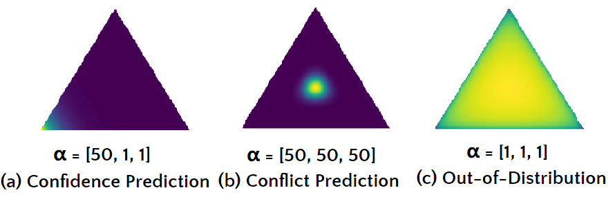
Figure 2: Illustration of different vacuity and dissonance of subjective opinions based on their evidence measures.

The main cause of vacuity (a.k.a. ignorance) is a lack of evidence or knowledge, which corresponds to uncertainty mass, $u_{Y}$, of an opinion in SL as:

$$\text{Vac}({\bm{\alpha}}_{Y})=\frac{W}{S}.$$ (6)

This type of uncertainty refers to uncertainty caused by insufficient information or knowledge to understand or analyze a given opinion.

The dissonance of an opinion can happen when there is an insufficient amount of evidence that can clearly support a particular belief. For example, when a same amount of evidence is supporting multiple extremes of beliefs, high dissonance is observed. Hence, the dissonance is estimated by the difference between singleton belief masses (e.g., class labels), leading to ‘inconclusiveness’ in decision making situations.

Given a multinomial opinion with non-zero belief masses, the measure of dissonance can be obtained by:

$$\text{Diss}({\bm{\alpha}}_{Y})=\sum\limits_{y_{i}\in\mathbb{Y}}\left(\frac{\bm{b}_{Y}(y_{i})\!\!\!\!\sum\limits_{y_{j}\in\mathbb{Y}\setminus y_{i}}\!\!\!\!\!\bm{b}_{Y}(y_{j})\mbox{Bal}(y_{j},y_{i})}{\sum\limits_{y_{j}\in\mathbb{Y}\setminus y_{i}}\bm{b}_{Y}(y_{j})}\right),$$ (7)

where the relative mass balance between a pair of belief masses $\bm{b}_{Y}(y_{j})$ and $\bm{b}_{Y}(y_{i})$ is expressed by:

$$\text{Bal}(y_{j},y_{i})=\begin{cases}1-\frac{|\bm{b}_{Y}(y_{j})-\bm{b}_{Y}(y_{i})|}{\bm{b}_{Y}(y_{j})+\bm{b}_{Y}(y_{i})},&\text{if $\bm{b}_{Y}(y_{j})\bm{b}_{Y}(y_{i})\neq 0$}\\ 0,&\text{otherwise.}\end{cases}$$ (8)

The above two uncertainty measures (i.e., vacuity and dissonance) can be interpreted using class-level evidence measures of subjective opinions. As in Fig. 2, given three classes (1, 2, and 3), we have three subjective opinions $\{{\bm{\alpha}}_{1},{\bm{\alpha}}_{2},{\bm{\alpha}}_{3}\}$, represented by the three-class evidence measures as: ${\bm{\alpha}}_{1}=(50,1,1)$ representing low uncertainty (entropy, dissonance and vacuity) which implies high certainty (often represented as high confidence in a decision making context), ${\bm{\alpha}}_{2}=(50,50,50)$ indicating high inconclusiveness due to high conflicting evidence which gives high entropy and high dissonance, ${\bm{\alpha}}_{3}=(1,1,1)$ showing the case of high vacuity which is commonly observed in OOD samples. Based on our observations from Fig 2 (b) and (c), we found that entropy cannot distinguish uncertainty due to vacuity or dissonance, which naturally results in inability to distinguish boundary samples from OOD samples. However, vacuity can effectively detect OOD samples because the cause of uncertainty is from a lack of evidence.

Evidential Neural Networks (ENNs)

ENNs (Sensoy, Kaplan, and Kandemir 2018) are similar to classical NNs except that the softmax layer is replaced by an activation layer (e.g., ReLU) to ascertain non-negative output, which is taken as the evidence vector for the predicted Dirichlet distribution. Given sample $i$, let $f({\bf x}_{i}|\Theta)$ represents the evidence vector predicted by the network for the classification, where ${\bf x}_{i}\in\mathbb{R}^{L}$ is the input feature and $\Theta$ is the network parameters. Then, the corresponding Dirichlet distribution has parameters ${\bm{\alpha}}_{i}=f({\bf x}_{i}|\Theta)+1$. Let ${\bf y}_{i}$ be the ground-truth label, the Dirichlet density $\text{Dir}({\bf p}_{i};{\bm{\alpha}})$ is the prior on the Multinomial distribution, $\text{Multi}({\bf y}_{i}|{\bf p}_{i})$. The following sum of squared loss is used to estimate the parameters ${\bm{\alpha}}_{i}$ based on the sample $i$:

$$\mathcal{L}(f({\bf x}_{i}|\Theta),{\bf y}_{i})=\int\frac{\|{\bf y}_{i}-{\bf p}_{i}\|_{2}^{2}}{B({\bm{\alpha}}_{i})}\prod_{j=1}^{K}p_{ij}^{(\alpha_{ij}-1)}d{\bf p}_{i}$$

$$=\sum_{j=1}^{K}(y_{ij}^{2}-2y_{ij}\mathbb{E}[p_{ij}]+\mathbb{E}[p_{ij}^{2}]).$$ (9)

Eq. (Evidential Neural Networks (ENNs)) is based on class labels of training samples. However, it does not directly measure the quality of the predicted Dirichlet distributions such that the uncertainty estimates may not be accurate.

Training ENNs with Wasserstein GAN

Given the various characteristics of uncertainty based on SL, we propose a novel model that combines ENNs and WGAN to quantify multiple types of uncertainty (i.e., vacuity and dissonance) and solving classification tasks.

Regularized ENNs

Given a set of samples $\mathcal{D}=\{({\bf x}_{1},{\bf y}_{1}),\cdots,({\bf x}_{N},{\bf y}_{N})\}$, let $P_{out}({\bf x},{\bf y})$ and $P_{in}({\bf x},{\bf y})$ be the distributions of the OOD and ID samples respectively. We propose a training method using a regularized ENN to minimize the following loss function over the parameters $\Theta$ of the model’s function $f$:

$$\mathcal{L}(\Theta)=\mathbb{E}_{{\bf x,\bf y}\sim P_{in}({\bf x,\bf y})}[\mathcal{L}(f({\bf x}|\Theta),{\bf y})]$$ (10)

$$-\beta\mathbb{E}_{{\bf\hat{x}}\sim P_{out}({\bf\hat{x}})}[\text{Vac}(f({\bf\hat{x}}|\Theta))].$$

The first item (Eq. (Evidential Neural Networks (ENNs))) ensures a good estimation of the class probabilities of the ID samples. Since it assigns large confidence on training samples during the classification process, it also contributes to reducing the vacuity of ID samples. The second item is to increase the vacuity estimation from the model on OOD samples. $\beta$ is the trade-off parameter. Therefore, minimizing Eq. (10) is to achieve high classification accuracy, low vacuity output for ID samples and high vacuity output for OOD samples. To ensure the model’s generalization to the whole data space, the choice of effective $P_{out}$ is important. While some methods (Lee et al. 2017; Hein, Andriushchenko, and Bitterwolf 2019; Sensoy et al. 2020) only use close or adversarial samples, we found that both close and far-away samples are equally important. Instead of using hand-picked auxiliary dataset $P_{out}$ which requires a lot of tuning (Zhao et al. 2019), we used generative models to provide sufficient various OOD samples.

Wasserstein Generators for OOD

We chose WGAN (Arjovsky, Chintala, and Bottou 2017) as our generators because (i) it provides higher stability than original GAN (Goodfellow et al. 2014); and (ii) it offers a meaningful loss metric by leveraging the Wasserstein distance, which can measure the distance between the generated samples and the ID region.

WGAN consists of two main components: Discriminator $D$ and generator $G$. $G$ maps input latent variable $z$ into generator output $G(z)$ where $D$ represents the probability of input sample ${\bf x}$ coming from ID. The objective function is to recover $P_{in}({\bf x})$ from $G$. WGAN uses the Wasserstein distance instead of the original divergence in the GAN’s loss function, which is considered as continuous and differentiable for optimization. The Wasserstein distance $dist(p,q)$ between two distributions $p$ and $q$ is informally defined as the minimum cost of transporting mass to transform $q$ into $p$. Under the Lipschitz constraint, the loss function of WGAN can be written as:

$$\min_{G}\max_{D}\mathbb{E}_{{\bf x}\sim P_{in}({\bf x})}\big{[}D({\bf x})\big{]}-\mathbb{E}_{\hat{{\bf x}}\sim P_{G}(z)}\big{[}D(\hat{{\bf x}})\big{]},$$ (11)

where $P_{in}$ is the ID and $P_{G}$ is the the generated distribution defined by $x=G(z)$ and $z\sim p(z)$, which is usually sampled from uniform or Gaussian noise distribution. WGAN employs weight clipping or gradient penalty (WGAN-GP) (Gulrajani et al. 2017) to enforce a Lipschitz constraint to keep the training stable. We can estimate the Wasserstein distance $dist$ at the step after $D$ updates and before $G$ updates during the alternating training process:

$$\mathbb{E}_{{\bf x}\sim P_{in}({\bf x})}\big{[}D({\bf x})\big{]}-\mathbb{E}_{\hat{{\bf x}}\sim P_{G}(z)}\big{[}D(\hat{{\bf x}})\big{]}.$$ (12)

The estimated curve of $dist$ during WGAN training shows high correlation with high visual quality of the generated samples (Arjovsky, Chintala, and Bottou 2017). When training WGAN from the scratch, the initial large distance indicates that the generated samples has very low-quality, showing far-away samples to the ID region. Through the progress of the training, the distance decreases continuously, which leads to higher sample quality. This implies that the samples are getting close to the ID region. Therefore we adopted $dist$ to measure the variety of generated samples, which are used as prior knowledge of our model.

However, original WGAN is designed to generate ID samples. To reinforce $G$ recover OOD $P_{out}$, we propose the following new WGAN loss with uncertainty regularization.

$$\min_{G}\max_{D}\mathbb{E}_{{\bf x}\sim P_{in}({\bf x})}\big{[}D({\bf x})\big{]}-\mathbb{E}_{\hat{{\bf x}}\sim P_{G}(z)}\big{[}D(\hat{{\bf x}})\big{]}$$ (13)

$$-\beta\mathbb{E}_{\hat{{\bf x}}\sim P_{G}(z)}\big{[}\text{Vac}(f({\bf\hat{\bf x}}|\Theta))\big{]},$$

where $\beta$ is a trade-off parameter and $\text{Vac}(f(\hat{\bf x}|\Theta))$ is the uncertainty estimation from a classifier trained on ID. This regularization item enforces the generated samples to have high vacuity uncertainty.

Jointly Training ENNs and WGAN

Algorithm 1 Alternating minimization for WGAN and ENN

Pretrained ENN with weights $\Theta$, initial $D$’s weights $\omega$, initial $G$’s weights $\theta$. $n_{d}$, $n_{e}$ : The number of iterations of $D$ and ENN per $G$ iteration. $\beta$: the trade-off weight. $m$: the batch size.

1:repeat

2:     for  $i=1,...,n_{d}$ do

3:         Sample $\{{\bf z}^{(i)}\}_{i=1}^{m}\!\sim\!P_{z}$ and $\{{\bf\hat{x}}^{(i)}\}_{i=1}^{m}\!\sim\!P_{G}(z)$

4:         Update $D$ by descending its gradient (with penalty)

5:   $\nabla_{\omega}\frac{1}{m}\sum\limits_{i=1}^{m}\big{[}D_{\omega}({\bf\hat{x}}^{(i)})\!-\!D_{\omega}({\bf x}^{(i)})+grad\_penalty\big{]}$

6:     end for

7:     Get the approximated Wasserstein distance

8:   $dist=\frac{1}{m}\sum\limits_{i=1}^{m}\big{[}D({\bf x}^{(i)})\!-\!D({\bf\hat{x}}^{(i)})\big{]}$

9:     Update $G$ once by ascending its gradient

10:   $\nabla_{\theta}\frac{1}{m}\sum\limits_{i=1}^{m}\big{[}\!D(G_{\theta}({\bf z}^{(i)}))+\beta\text{Vac}(f(G_{\theta}({\bf z}^{(i)})|\Theta))\big{]}$

11:     for  $i=1,...,n_{e}$ do

12:         Sample $\{{\bf x}^{(i)},{y}^{(i)}\}_{i=1}^{m}\!\sim\!P_{in}$, $\{{\bf z}^{(i)}\}_{i=1}^{m}\!\sim\!P_{z}$ , $\{{\bf\hat{x}}^{(i)}\}_{i=1}^{m}\!\sim\!P_{G}(z)$

13:         Update ENN by descending the gradient

14:   $\nabla_{\Theta}\frac{1}{m}\sum\limits_{i=1}^{m}\big{[}\mathcal{L}(f({\bf x}^{(i)}|\Theta),y^{(i)})\big{]}$

15:         Update ENN by ascending the gradient

16:   $\nabla_{\Theta}\frac{\beta}{m}\sum\limits_{i=1}^{N}\big{[}\text{Vac}(f({\bf\hat{x}}^{(i)}|\Theta))\big{]}$

17:     end for

18:until $dist$ convergence

To improve the OOD detection accuracy, we jointly trained regularized ENN loss (Eq. (10)) and WGAN-GP with uncertainty regularization (Eq. (13)) in Algorithm 1. This allows ENNs to utilize various types of OOD samples generated from WGAN. We usually pretrain the ENN classifier for a good classification accuracy to accelerate the training.

Each batch of the OOD samples correspond to different decreasing $dist$. This enables the ENN to utilize a wide range of OOD samples. ENNs improves uncertainty estimation based on OOD samples from $P_{G}$, and $G$ achieves a better OOD quality due to uncertainty estimation from ENNs simultaneously. We stop the training when $dist$ converges in case the ENN may forget the effect of previous far-away OOD samples from ID regions. Fig 6 illustrates the change of $dist$ and output vacuity during the training process.

Experiments

We first illustrated the advantage of evidential uncertainty in (1) a synthetic experiment. Then we compared our approach with the recent uncertainty estimation models on (2) predictive uncertainty estimation and (3) adversarial uncertainty estimation. (4) We also investigated the effect of different types of uncertainties on the OOD detection.

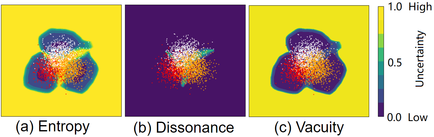
Figure 3: A synthetic experiment that shows the benefit of using evidential uncertainties (vacuity, dissonance) over entropy ranged in [0, 1]. Entropy cannot distinguish ID and OOD samples at class boundaries.

Synthetic

Fig 3 shows three Gaussian distributed classes with equidistant means and tied isotropic variance $\sigma^{2}=4$ (a large degree of class overlap). We used our proposed WENN method, a small NN with 2 hidden layer of 500 neurons each was trained on this data. Fig 3 demonstrates that entropy and two evidential uncertainties, which are vacuity, dissonance, exhibit distinctive behaviors. Entropy is high both in overlapping and far-away regions from training data, which makes it hard to distinguish ID and OOD samples at class boundaries. In contrast, vacuity is low over the whole region of training data while vacuity is high for the outside of the region of training data. This allows the ID region to be clearly distinguished from the OOD region. In addition, high dissonance is observed over decision boundary which indicates high chances of misclassification.

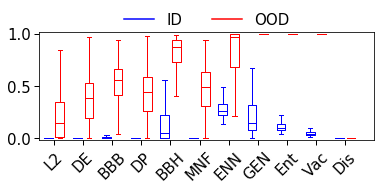
(a) MNIST: ID vs OOD

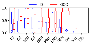
(b) CIFAR10: ID vs OOD

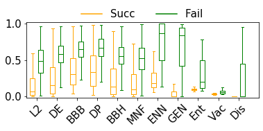
(c) CIFAR10: Successful vs Fail predictions

Figure 4: Boxplots of predictive uncertainty of different models on ID/OOD testing datasets: (a) MNIST test set (ID) vs notMNIST (OOD); (b) Samples from the first five (ID) vs the last five (OOD) categories of CIFAR10 test set; (c) Successful and failed predictions in CIFAR10 test set (ID). Our model uses entropy (Ent), vacuity (Vac), dissonance (Dis) as a measure of uncertainty, while other models use entropy.

Predictive Uncertainty Estimation

Comparing Schemes: We compared our model with the following schemes: (i) L2 refers to the standard deterministic NNs with softmax output and weight decay; (ii) DP uses Dropout, the uncertainty estimation model (i.e., BNNs) (Gal and Ghahramani 2016); (iii) DE refers to Deep Ensembles (Lakshminarayanan, Pritzel, and Blundell 2017); (iv) BBB refers to Bayes by Backprop  (Blundell et al. 2015); (v) BBH refers to Bayes by Hypernet (Pawlowski et al. 2017), a Bayesian model based on implicit weight uncertainty; (vi) MNF refers to the variational approximation based model in (Louizos and Welling 2017); (vii) ENN uses evidential DL model (Sensoy, Kaplan, and Kandemir 2018); (viii) GEN combines ENNs and Adversarial Autoencoder (Sensoy et al. 2020); and (ix) Ent, Vac and Dis are the entropy, vacuity and dissonance of our proposed model WENN.

Setup: We followed the same experiments in (Sensoy et al. 2020) on MNIST (LeCun et al. 1998) and CIFAR10 (Krizhevsky 2012): (1) For the MNIST dataset, we used the same LeNet-5 architecture from (Sensoy et al. 2020). We trained the model on MNIST training set and tested on MNIST testing set as ID samples and notMNIST (Bulatov, Y. 2011) as OOD samples; and (2) For the CIFAR10 dataset, we used ResNet-20 (He et al. 2016) as a classifier in all the models considered in this work. We trained on the samples for the first five categories {airplane, automobile, bird, cat, deer} in the CIFAR10 training set (i.e., ID), while using the other five categories {ship, truck, dog, frog, horse} as testing OODs. We used the source code of BBH and GEN, which also contained implementations of other approaches. But we changed all the classifiers to the same LeNet-5 and ResNet-20 respectively. All the baselines were fairly trained with their default best parameters and we reported the average results. For WENN, we set $\beta=0.1$, $n_{d}=2$, $n_{e}=1$, $m=256$, $\mathrm{learning\_rate}=1e^{-4}$ in Algorithm 1 in all the experiments, which were fine-tuned considering the performance of both the OOD detection and ID classification accuracy. For more details refer to Appendix and our source code .

Metrics: Our proposed model used vacuity and dissonance estimated based on Eq. (6) and Eq. (7). To be consistent with other works that used entropy as a measure of uncertainty, we also compared the predictive entropy over the range of possible entropy $[0,1]$. We used the boxplots to show the distribution of predictive uncertainty.

Results: To evaluate OOD uncertainty qualification, Fig 4 (a) and (b) show the boxplots of the predictive uncertainty under all models trained with MNIST and CIFAR10 and tested on their corresponding ID and OOD datasets. The ideal model is expected to have a low ID box and a high OOD box, i.e., the model is certain about the ID inputs while totally uncertain about the OOD inputs. To measure ID uncertainty qualification, Fig 4 (c) shows the boxplots of different models’ predictive uncertainty for correct and mis-classified examples in CIFAR10 ID testing set. The figure indicates that a standard network is overconfident of any inputs. BBH performs the best among all the Bayesian models on MNIST but fails to give a disparity between ID and OOD on CIFAR10. ENN and GEN perform well on MNIST. However, Fig 4 (b) and (c) show that they force high uncertainty for mis-classified ID samples the same as OOD samples on CIFAR10. (Sensoy et al. 2020) admits that ENN and GEN may classify the boundary ID samples as OOD because of their high entropy. The above results all indicate the limitation of entropy in uncertainty estimation.

WENN using entropy beats other counterparts in estimating OOD uncertainty because it benefits from our algorithm using vacuity. However, WENN is more powerful when using vacuity and dissonance to measure OOD and ID uncertainty respectively. For ID uncertainty, Fig 4 (c) illustrates that high dissonance implies conflicting evidence, which can result in mis-classification. For OOD uncertainty, Fig 4 (b) and (c) show that all the ID samples, i.e., even the mis-classified samples, have extreme low vacuity, compared to the high vacuity of OOD samples. However, WENN still assigns medium entropy to boundary ID samples. This is consistent with the synthetic experiment’s result, showing the advantage of adopting vacuity in distinguishing boundary ID and OOD samples.

Adversarial Uncertainty Estimation

We also evaluated these models on CIFAR10 using adversarial examples generated by FGSM (Goodfellow, Shlens, and Szegedy 2014) with different perturbation values $\epsilon\!\in\![0,0.5]$. DE is excluded because it is trained on adversarial samples. Fig 6 shows that as $\epsilon$ increases, WENN’s accuracy immediately drops to random and the uncertainty simultaneously increases to maximum entropy, i.e., WENN will assign the highest uncertainty with the inputs if it can’t make easy predictions. It knows what it doesn’t know and never becomes overconfident. We observe the same behaviors for MNIST dataset (in Appendix).

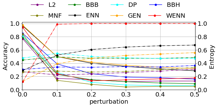
Figure 5: Accuracy (solid) vs entropy (dashed) as a function of the adversarial perturbation $\epsilon$ on CIFAR10.

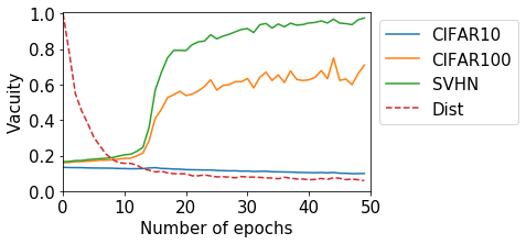
Figure 6: The change of normalized Wasserstein distance and the vacuity of ID/OOD samples when trained on CIFAR10.

ID*	OOD	MSP	ENN	GEN	CCC	ODIN	ACET	OE	CCU	Ent	Vac
FMNIST	MNIST	96.9	90.1	96.2	99.9	99.2	95.6	92.0	96.2	100.0	100.0
	notMNIST	87.5	87.8	93.6	96.4	90.2	92.4	93.0	96.7	99.9	100.0
	Uniform	93.0	91.6	96.9	95.4	94.9	100.0	99.3	100.0	99.9	100.0
CIFAR10	CIFAR100	86.3	75.0	84.0	84.0	87.1	85.2	86.0	92.5	98.6	99.5
	SVHN	88.9	78.6	85.4	80.5	85.1	89.6	92.1	98.9	100.0	100.0
	LSUN_CR	88.8	64.4	98.0	99.7	92.8	89.1	92.7	98.6	100.0	100.0
	Uniform	93.8	84.6	82.4	82.4	99.3	100.0	100.0	100.0	100.0	100.0
SVHN	CIFAR10	95.2	52.9	50.2	98.6	95.8	96.3	100.0	100.0	99.3	100.0
	CIFAR100	94.9	51.8	51.0	98.2	95.3	95.6	100.0	100.0	99.3	100.0
	LSUN_CR	94.9	55.5	53.9	100.0	95.6	97.0	100.0	100.0	99.8	99.9
	Uniform	95.8	53.9	53.2	100.0	96.6	100.0	100.0	100.0	99.8	100.0

Table 1: AUROC for OOD detection. ID: in-distribution samples, OOD: out-of-distribution samples.

Out-of-Distribution Detection

Comparing Schemes: We compared with several recent methods specifically designed for OOD detection, together with uncertainty models ENN and GEN: (i) MSP refers to maximum softmax probability, a baseline of OOD detection in (Hendrycks and Gimpel 2016); (ii) CCC (Lee et al. 2017) uses GAN to generate boundary OOD samples as regularizers; (iii) ODIN calibrates the estimated confidence by scaling the logits before softmax layers (Liang, Li, and Srikant 2017); (iv) ACET uses adversarial examples to enhance the confidence (Hein, Andriushchenko, and Bitterwolf 2019); (v) OE refers to Outlier Exposure (Hendrycks, Mazeika, and Dietterich 2018) that enforces uniform confidence on 80 million Tiny ImageNet (Torralba, Fergus, and Freeman 2008); (vi) CCU integrates Gaussian mixture models in OOD detection DL models (Meinke and Hein 2019); and (vii) Ent and Vac refer to our WENN model using entropy or vacuity as scores.

Setup: We used FashionMNIST (Xiao, Rasul, and Vollgraf 2017), notMNIST, CIFAR10, CIFAR100 (Krizhevsky 2012), SVHN (Netzer et al. 2011), the classroom class of LSUN (i.e., LSUN_CR) (Yu et al. 2015) and uniform noise as ID or OOD datasets. We used the source code in (Meinke and Hein 2019) which contained implementations of other baselines, but we used ResNet-20 for all the models except CCC. We used VGG-13 (Simonyan and Zisserman 2014) for CCC because we couldn’t achieve an acceptable accuracy using ResNet-20. And ODIN, OE and CCU were directly trained or calibrated on the Tiny ImageNet. Other settings were the same as the previous uncertainty estimation experiments.

Metrics: Our model uses vacuity to distinguish between ID and OOD samples. ENN and GEN use the entropy of the predictive probabilities as recommended in their papers. The other methods use their own OOD scores. We use area under the ROC (AUROC) curves to evaluate the performance of different type of uncertainty.

Results: Table 1 shows the AUROC curves performance of different approaches. WENN’s vacuity beats all the other uncertainty scores, including its own entropy. ENN and GEN are not originally designed for OOD detection because they assign the same high entropy to mis-classified ID samples as OOD. CCC doesn’t generalize well and it lacks scalability to recent deep architectures like ResNet to ensure a better classification accuracy. The result of ACET proves that the effect of using purely close adversarial examples is limited. (Hein, Andriushchenko, and Bitterwolf 2019) admits that ACET will yield high-confidence predictions far away from the training data. ODIN, OE and CCU are directly trained or tuned using a large auxiliary dataset which should contain both far-away and close samples. The outperformance of WENN indicates that our algorithm using vacuity can generate and utilize sufficient OOD samples more effectively.

To further explain how our model generates and utilizes variable OOD samples, Fig 6 illustrates the alternating optimization process when the model is trained on CIFAR10 training set. The initial ENN classifier is overconfident and assigns arbitrary inputs with low vacuity 0.2. As the Wasserstein distance decreases gradually, implying that the generated samples keep moving from far-away to closer to the ID region, the model learns to output low vacuity on ID samples from CIFAR10 testing set and high vacuity on OOD samples from CIFAR100 and SVHN. The output vacuity of CIFAR100 is lower than that of SVHN. This indicates vacuity is a reasonable uncertainty metric because CIFAR100 is often considered as near-distribution outliers of CIFAR10. However, the medium vacuity of CIFAR100 is still good enough for perfect classification.

Conclusion

We proposed a novel DL model, called WENN that combines ENNs with WGAN, to jointly train a model with prior knowledge of a certain class (i.e., high vacuity OOD samples). Via extensive experiments based on both synthetic and real datasets, we proved that: (1) vacuity can distinguish boundary samples from OOD samples; (2) the proposed model with vacuity regularization can produce and utilize various types of OOD samples successfully. Our model achieved the state of the art performance in both uncertainty estimation and OOD detection benchmarks.

References

- Arjovsky, Chintala, and Bottou (2017) Arjovsky, M.; Chintala, S.; and Bottou, L. 2017. Wasserstein gan. arXiv preprint arXiv:1701.07875 .
- Blundell et al. (2015) Blundell, C.; Cornebise, J.; Kavukcuoglu, K.; and Wierstra, D. 2015. Weight uncertainty in neural networks. arXiv preprint arXiv:1505.05424 .
- Bulatov, Y. (2011) Bulatov, Y. 2011. notMNIST dataset. http://yaroslavvb.blogspot.it/2011/09/notmnist-dataset.html. Last accessed on 03/02/2021.
- De Silva (2018) De Silva, C. W. 2018. Intelligent control: fuzzy logic applications. CRC press.
- Gal (2016) Gal, Y. 2016. Uncertainty in deep learning. University of Cambridge .
- Gal and Ghahramani (2016) Gal, Y.; and Ghahramani, Z. 2016. Dropout as a Bayesian approximation: Representing model uncertainty in deep learning. In ICML, 1050–1059.
- Goodfellow et al. (2014) Goodfellow, I.; Pouget-Abadie, J.; Mirza, M.; Xu, B.; Warde-Farley, D.; Ozair, S.; Courville, A.; and Bengio, Y. 2014. Generative adversarial nets. In NIPS, 2672–2680.
- Goodfellow, Shlens, and Szegedy (2014) Goodfellow, I. J.; Shlens, J.; and Szegedy, C. 2014. Explaining and harnessing adversarial examples. arXiv preprint arXiv:1412.6572 .
- Gulrajani et al. (2017) Gulrajani, I.; Ahmed, F.; Arjovsky, M.; Dumoulin, V.; and Courville, A. C. 2017. Improved training of wasserstein gans. In NIPS, 5767–5777.
- He et al. (2016) He, K.; Zhang, X.; Ren, S.; and Sun, J. 2016. Deep residual learning for image recognition. In CVPR, 770–778.
- Hein, Andriushchenko, and Bitterwolf (2019) Hein, M.; Andriushchenko, M.; and Bitterwolf, J. 2019. Why ReLU networks yield high-confidence predictions far away from the training data and how to mitigate the problem. In CVPR, 41–50.
- Hendrycks and Gimpel (2016) Hendrycks, D.; and Gimpel, K. 2016. A baseline for detecting misclassified and out-of-distribution examples in neural networks. arXiv preprint arXiv:1610.02136 .
- Hendrycks, Mazeika, and Dietterich (2018) Hendrycks, D.; Mazeika, M.; and Dietterich, T. 2018. Deep anomaly detection with outlier exposure. arXiv preprint arXiv:1812.04606 .
- Jøsang (2016) Jøsang, A. 2016. Subjective logic. Springer.
- Jøsang, Cho, and Chen (2018) Jøsang, A.; Cho, J.-H.; and Chen, F. 2018. Uncertainty Characteristics of Subjective Opinions. In Fusion, 1998–2005. IEEE.
- Kendall and Gal (2017) Kendall, A.; and Gal, Y. 2017. What uncertainties do we need in Bayesian deep learning for computer vision? In NIPS, 5574–5584.
- Krizhevsky (2012) Krizhevsky, A. 2012. Learning Multiple Layers of Features from Tiny Images. University of Toronto .
- Lakshminarayanan, Pritzel, and Blundell (2017) Lakshminarayanan, B.; Pritzel, A.; and Blundell, C. 2017. Simple and scalable predictive uncertainty estimation using deep ensembles. In NIPS, 6402–6413.
- LeCun et al. (1998) LeCun, Y.; Bottou, L.; Bengio, Y.; and Haffner, P. 1998. Gradient-based learning applied to document recognition. Proceedings of the IEEE 86(11): 2278–2324.
- Lee et al. (2017) Lee, K.; Lee, H.; Lee, K.; and Shin, J. 2017. Training confidence-calibrated classifiers for detecting out-of-distribution samples. arXiv preprint arXiv:1711.09325 .
- Liang, Li, and Srikant (2017) Liang, S.; Li, Y.; and Srikant, R. 2017. Enhancing the reliability of out-of-distribution image detection in neural networks. arXiv preprint arXiv:1706.02690 .
- Louizos and Welling (2017) Louizos, C.; and Welling, M. 2017. Multiplicative normalizing flows for variational bayesian neural networks. In Proceedings of the 34th International Conference on Machine Learning, volume 70, 2218–2227. JMLR. org.
- Malinin and Gales (2018) Malinin, A.; and Gales, M. 2018. Predictive Uncertainty Estimation via Prior Networks. arXiv preprint arXiv:1802.10501 .
- Meinke and Hein (2019) Meinke, A.; and Hein, M. 2019. Towards neural networks that provably know when they don’t know. arXiv preprint arXiv:1909.12180 .
- Netzer et al. (2011) Netzer, Y.; Wang, T.; Coates, A.; Bissacco, A.; Wu, B.; and Ng, A. 2011. Reading Digits in Natural Images with Unsupervised Feature Learning. NIPS .
- Pawlowski et al. (2017) Pawlowski, N.; Brock, A.; Lee, M. C.; Rajchl, M.; and Glocker, B. 2017. Implicit weight uncertainty in neural networks. arXiv preprint arXiv:1711.01297 .
- Sensoy et al. (2020) Sensoy, M.; Kaplan, L.; Cerutti, F.; and Saleki, M. 2020. Uncertainty-Aware Deep Classifiers using Generative Models. arXiv preprint arXiv:2006.04183 .
- Sensoy, Kaplan, and Kandemir (2018) Sensoy, M.; Kaplan, L.; and Kandemir, M. 2018. Evidential deep learning to quantify classification uncertainty. In NIPS, 3183–3193.
- Sentz, Ferson et al. (2002) Sentz, K.; Ferson, S.; et al. 2002. Combination of evidence in Dempster-Shafer Theory, volume 4015. Citeseer.
- Shannon (1948) Shannon, C. E. 1948. A mathematical theory of communication. The Bell system technical journal 27(3): 379–423.
- Simonyan and Zisserman (2014) Simonyan, K.; and Zisserman, A. 2014. Very deep convolutional networks for large-scale image recognition. arXiv preprint arXiv:1409.1556 .
- Torralba, Fergus, and Freeman (2008) Torralba, A.; Fergus, R.; and Freeman, W. T. 2008. 80 million tiny images: A large data set for nonparametric object and scene recognition. IEEE transactions on pattern analysis and machine intelligence 30(11): 1958–1970.
- Xiao, Rasul, and Vollgraf (2017) Xiao, H.; Rasul, K.; and Vollgraf, R. 2017. Fashion-mnist: a novel image dataset for benchmarking machine learning algorithms. arXiv preprint arXiv:1708.07747 .
- Yu et al. (2015) Yu, F.; Seff, A.; Zhang, Y.; Song, S.; Funkhouser, T.; and Xiao, J. 2015. Lsun: Construction of a large-scale image dataset using deep learning with humans in the loop. arXiv preprint arXiv:1506.03365 .
- Zhao et al. (2019) Zhao, X.; Ou, Y.; Kaplan, L.; Chen, F.; and Cho, J.-H. 2019. Quantifying Classification Uncertainty using Regularized Evidential Neural Networks. arXiv preprint arXiv:1910.06864 .