Generative Neural Samplers for the Quantum Heisenberg Chain
Abstract
Generative neural samplers offer a complementary approach to Monte Carlo methods for problems in statistical physics and quantum field theory. This work tests the ability of generative neural samplers to estimate observables for real-world low-dimensional spin systems. It maps out how autoregressive models can sample configurations of a quantum Heisenberg chain via a classical approximation based on the Suzuki-Trotter transformation. We present results for energy, specific heat and susceptibility for the isotropic XXX and the anisotropic XY chain that are in good agreement with Monte Carlo results within the same approximation scheme.
I Introduction
Monte Carlo methods are the most important numerical techniques for gaining insights in statistical mechanics systems and lattice field theories from first principles mc_newman ; gattringer_lang . Despite their success, Monte Carlo methods come with some drawbacks. They often suffer from long auto-correlation times, especially close to criticality. Moreover, they can get trapped in a subset of configuration space which hinders them from sampling all relevant parts of the space.
Generative neural samplers (GNSs) are deep learning models that can sample from an explicitly or implicitly learned probability distribution. They were successfully used to model complicated real-world distributions in applications like text-to-speech or image synthesis. Recently, they have been applied to a variety of problems in statistical physics and lattice field theory. Some approaches rely on samples from a Monte Carlo algorithm for training while others are completely independent from Monte Carlo methods. GNS models of the first-mentioned category have been used for example to estimate the thermodynamics of the Ising model in two dimensions thermodynamics_BM ; DL_Ising ; GAN_ising ; ising_field_VAE . Representatives of the latter category are autoregressive models or normalizing flows and offer a truly complementary approach to Monte Carlo methods. In wu_solving_stat_mech , autoregressive models were applied to the two-dimensional classical Ising and Sherrington-Kirkpatrick model. The approach was advanced in nicoli2019comment ; kim_savan by bringing forward an asymptotically unbiased estimator for GNSs that provide the exact sampling probability.
In the domain of quantum systems, GNS have been used for the study of ground-state properties, offering an alternative approach to methods like Variational Monte Carlo or Green’s function Monte Carlo. In BM_Carleo ; BM_Carleo_2 ; BM_noe ; BM_groundstate1 ; DNN_groundstate , GNS have shown the ability to represent the ground-state of quantum many-body-systems. Moreover, GNS have found application in the domain of lattice field theories, like for the -theory zhou2019regressive ; phi4_urban ; phi4_shanahan ; nicoli2020estimation and for the -gauge theory lft_u1 and -gauge theory lft_SUN in two dimensions.
In this work, the journey towards autoregressive models for the thermodynamics of quantum mechanical statistical models is taken. Here, the quantum Heisenberg chain in two special cases serves as an example. This system is approximately realized in real materials Ising_realization ; XY_realization ; XXZ_realization ; realization_QPT and is a key model in studying quantum phase transitions or the dynamics of correlated lattice systems QPT_1 ; QPT_2 ; santos_dynamics .
The paper is organized as follows: Section II gives a short overview of the quantum Heisenberg chain, maps out the Suzuki-Trotter transformation, which is used here to approximate the quantum Heisenberg chain by a classical system, and explains how samples from the classical approximation can be drawn by a GNS model. Section III examines the estimates for internal energy, specific heat and susceptibility of the isotropic and XY Heisenberg chain. We summarize and conclude in Section IV. Technical details and derivations were included in several appendices to make the paper self-contained.
II Generative neural samplers for the Heisenberg chain
II.1 Heisenberg chain
The general spin- Heisenberg chain with nearest-neighbor coupling and without an external field is described by the Hamiltonian
| (1) |
Here, are the spin operators that act on each site and fulfill the commutation relations . are real-valued coupling constants and we assume periodic boundary conditions by identifying . The spin- Heisenberg chain is solved exactly by the Bethe Ansatz in the sense that the spectrum of the Hamiltonian is described exactly by the Bethe equations bethe_original . Because of the increasing computational complexity of identifying all Bethe solutions when this knowledge about the spectrum of the Hamiltonian does not enable a direct quantification of the thermodynamic behavior. To do so, numerical calculations for finite-size systems can be used and extrapolated to infinite chains, like in the pioneering work of calc_bonnerfisher_64 with chain lengths up to . Two well-known methods to derive the thermodynamic quantities of the XXX chain are the thermal Bethe Ansatz developed by tba_takahashi and the Quantum Transfer Matrix Method pioneered by QMT_start_koma ; QMT_start_suzuki .
In this work, we study two special cases: The ferromagnetic XXX Heisenberg chain with and the ferromagnetic XX-chain with and , a special case of the XY-chain. In the case of the XY-chain, where the coupling between the -spin components is turned off in Equation 1, an analytical solution of the free energy is available. It was first obtained by xy_LSM , who applied a Jordan-Wigner transformation under which the XY chain reduces to a system of free spinless fermions. Shortly after, xysol_katsura_62 used a different procedure to write the Hamiltonian of the XY chain with a transverse external field in terms of fermion creation and annihilation operators. The resulting expression for the free energy of a chain of spins with periodic boundary conditions in the limit and without a magnetic field is
| (2) |
where and . The GNS results of this work will mainly be compared to results from a Markov Chain Monte Carlo (MCMC) algorithm by mc_cullenlandau_83 , which is described in Appendix E. It is based on the mapping of the quantum spin chain to a classical two-dimensional system discussed below and a special update routine.
II.2 Suzuki-Trotter transformation
In order to apply GNSs to the quantum Heisenberg chain, the Suzuki-Trotter decomposition is used to transform the partition function of the quantum spin system,
| (3) |
into the partition function of a two-dimensional Ising-like classical system checkerboard_barma_78 ; mc_cullenlandau_83 ,
| (4) |
with . The caret denotes that the sum is running over terms with and both odd or both even and are eigenvalues of the Ising part of in Equation 1. The matrix elements couple four spins and are found in Appendix B. The derivation of Equation 4 is mapped out in Appendix B. Equation 4 can be interpreted as the partition function of an Ising system with two-spin interactions along the real space direction and temperature-dependent four-spin interactions on the alternating plaquettes marked blue in Figure 1 that couple neighboring spins in both the real direction and the Trotter direction . When evaluating the matrix elements in Appendix B one finds that only of the possible cases for a 4-spin plaquette are non-zero, namely those with an even number of spins in each direction. Only configurations that contain just the non-zero 4-spin plaquettes are allowed, as configurations violating these constraints would have infinite energy or zero contribution to the partition function otherwise. From Equation 29 one can read of that the trace operation in requires periodic boundary conditions in the Trotter direction. Following mc_cullenlandau_83 , periodic boundary conditions are also used in the real space direction. The eight allowed 4-spin plaquettes are depicted in Figure 1. Their energies, including the 2-spin interaction from the first term and the 4-spin interaction from the second term in Equation 4, are
| (5) | ||||
| (6) | ||||
| (7) | ||||
| (8) |
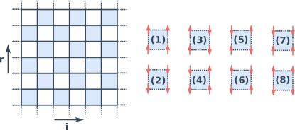
When , and hence diverges. Thus, only configurations that contain the 4-spin plaquettes - are allowed in this case.
II.3 Thermal averages
The thermal properties of the classical system above can be found by taking the respective derivatives of the free energy. The resulting expressions differ from the naive ones due to the temperature-dependent interactions in the effective Hamiltonian mc_cullenlandau_83 . The thermal average of the internal energy is
| (9) |
where is the non-trivial energy function in the th state whose ensemble average is the thermal average, i.e.
| (10) |
From there, the specific heat can be derived,
| (11) |
with
| (12) |
The parallel susceptibility is obtained as
| (13) |
where
| (14) |
A detailed derivation of these thermal averages and the contributions of an individual plaquette to , and are given in Appendix C.
II.4 Autoregressive models
This work focuses on autoregressive models which form a subclass of GNSs. They provide the exact probability with which a configuration is sampled, where parameterizes the sampler. To model for an -dimensional distribution an ordering of the components of is specified. The one-dimensional conditional distributions are modeled by a neural network. The joint probability is the product of the conditional distributions over all components,
| (15) |
and a sample can be drawn from by sequentially sampling from the corresponding conditional distributions. Autoregressive models can be trained by minimizing the inverse Kullback-Leibler divergence between the Boltzmann distribution and the variational distribution ,
| (16) |
without resorting to Monte-Carlo configurations. The expression can be straightforwardly optimized by gradient descent upon noting the that last term, , only represents an irrelevant constant in this respect. In this work, we use a PixelCNN vdoord_pcnn to model the conditional distributions , which was developed in the context of natural image generation. In wu_solving_stat_mech ; nicoli2019comment ; kim_savan it was applied to classical two-dimensional spin systems.
II.5 Sampling configurations
The mapped Heisenberg model only allows the 4-spin configurations depicted in Figure 1. When a autoregressive model samples a configuration spin-by-spin and row-by-row, the outcome will in general include illegal plaquettes. In early tests, a high energy was assigned to these configurations as a penalty term to see whether the model would learn to avoid sampling illegal configurations. This led to a quick collapse of the training and the model would learn to only sample either spins up () or spins down (). The strategy used instead was to change the sampling procedure such that only configurations with exclusively legal plaquettes are generated. In this procedure, the spins are sampled row-by-row, but only if the value of a spin is not determined by the condition to generate only legal plaquettes. For a plaquette in the center for example, only the first three spins of a plaquette are sampled. The fourth spin is determined by the product of the first three spins as the product of all four spins is required to be positive. When using this modified sampling procedure, only the conditional probabilities that were used to sample a spin contribute to the joint probability and Equation 15 changes to
| (17) |
mc_cullenlandau_83 applied their Monte Carlo method to systems with where plaquettes (7) and (8) are forbidden. It is not possible to construct a sequential sampling procedure that produces configurations with only the first six plaquettes from Figure 1 that obeys the periodic boundary conditions in both directions. To circumvent this problem, very similar systems with with are studied. For the XY chain, the analytical solutions for the internal energy , specific heat and susceptibility by Katsura xysol_katsura_62 in Equations 18, 19 and A show that there is basically no difference between nd .
III Results
Following mc_cullenlandau_83 , Heisenberg chains of length were investigated, where finite size effects are small compared to statistical errors in the Monte Carlo data. The GNS samplers were tested for and , corresponding to approximate classical systems on and grids, respectively. Next to the simple sample mean in Equation 60, the asymptotically unbiased Neural Importance Sampling (NIS) estimator in Equation 61 by nicoli2019comment ; kim_savan is evaluated for each observable. The experimental details are listed in Appendix F.
III.1 XY chain
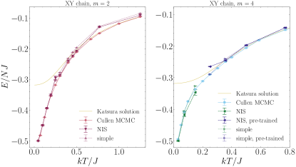
In Figures 2 and 3, the GNS estimates for internal energy , specific heat and susceptibility of an XY chain with are compared to those of the MCMC algorithm described in Appendix E. The analytical solution by Katsura xysol_katsura_62 is given for completeness. For this system, the difference between the ground-state of the quantum system and the classical approximation is large at low temperatures, where the quantum effects are poorly reproduced by the classical approximation with and , respectively. This equally affects the GNS as well as the MCMC results.
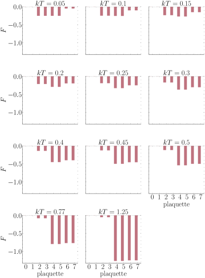
The NIS estimates for the internal energy are in reasonable agreement with the MCMC estimates within errorbars at most temperatures for , only at the NIS estimate differs considerably and is not compatible with the MCMC result within errorbars. Here, the errors for the MCMC results were estimated according to wolff_error . The simple sample averages for the internal energy are quite accurate at low temperatures, but deviate with increasing temperature. This reflects the difficulty of estimating at higher temperatures, which can be understood as follows: Figure 6 shows the contributions of each plaquette type from Figure 1 to the energy function at different temperatures. At low temperatures, the contributions of plaquettes do not differ much. With increasing temperature, the gap between the contributions of plaquettes and plaquettes widens. Plaquettes and are not relevant for as they have a vanishing probability of occurring. Configurations with a high number of plaquettes make a large contribution to the estimate while having a very low probability as can be read off from Equation 7. Learning to sample these rare configurations is a difficult task. This could explain the bad simple estimate at . At this temperature, also the NIS estimate does not agree with the MCMC estimate.
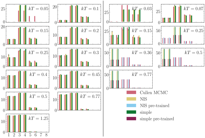
The specific heat of the classical system has a peak around . The NIS estimates on the descending part of the peak have a large variance but are reasonable. A comparison to the MCMC estimates is only partly possible due to their large statistical errors, which are too large to fit into the plot at temperatures below and only become reasonably small at . At higher temperatures, all NIS estimates are compatible with the MCMC estimates and show less variance. The simple estimates for follow the MCMC estimates only qualitatively around the peak but are more accurate towards higher temperatures. The NIS estimate at is poor because the model samples only configurations in the ground-state which consists of and plaquettes. This can be seen in Figure 9, which shows the average number of plaquettes of each type across all samples.
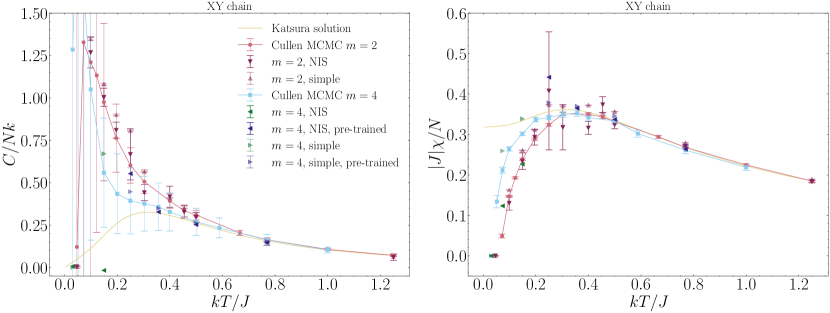
Similar to the specific heat, the NIS estimates for the susceptibility have a large variance for temperatures and for . At temperatures and , the NIS estimates with error bounds do not agree with the MCMC estimates. This changes at higher temperatures, where NIS estimates are compatible with the MCMC estimates. Again, the simple sample estimates only follow the MCMC estimates qualitatively, reiterating the importance of using NIS estimates instead of simple means nicoli2019comment ; kim_savan .
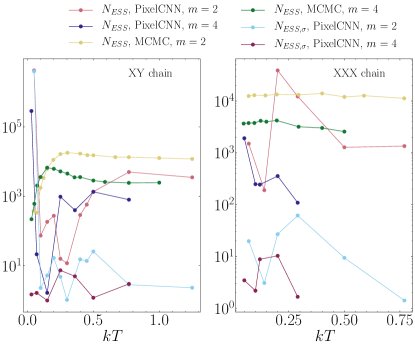
It is instructive to evaluate the effective sample sizes for the point estimate in Equation 66 and its variance as defined in Equation 67 along the lines of mcbook , which are shown in Figure 7. is particularly small for and for . This could explain why the NIS estimates for and at these temperatures are poor. Most notably, is only one at . The lower limit for the effective sampling sizes above which the estimate is still trustworthy is not clear. Although and at and are not as low as at other temperatures for , the NIS estimates of are bad at these temperatures. However, the effectiveness of importance sampling also depends on the function that is sampled which is not taken into account by and .
For , the estimates of a PixelCNN model trained as outlined in Appendix F are reasonable up to only . At higher temperatures, the model collapses into either sampling only ground-state configurations or exclusively configurations of only or plaquettes. This can be seen in Figure 9. Fortunately, the PixelCNN could be prevented from collapsing by using a pretraining schedule. For the model at , training of the model at was continued for epochs. The resulting model was then used as a pretrained model for the one at . This procedure was iterated up to .
III.2 Isotropic (XXX) chain
Figures 4 and 5 show PixelCNN estimates for the internal energy , specific heat and susceptibility of an almost isotropic chain with approximated by a classical system with and . They are compared to those of the MCMC algorithm described in Appendix E. The finite-size calculations for the quantum system by Bonner and Fisher calc_bonnerfisher_64 are given for reasons of completeness. The ground-state energy of the quantum system and the classical approximation are equal. This is why for low temperatures, the MCMC results are quite close to the Bonner-Fisher-curve, considering the small extension in Trotter direction of the classical approximation.
For the PixelCNN model performs well in estimating the internal energy , specific heat and susceptibility up to a certain temperature. The NIS estimates agree with the MCMC estimates within error bounds for all observables and temperatures except for at . The simple sample mean estimates only follow the MCMC estimates for and qualitatively. For , the deviation between these estimates increases with temperature.
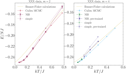
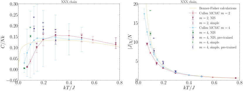
Interestingly, for , the simple estimates are quite close to the MCMC estimates. For this observable, only plaquettes contribute to the sum. Apparently, the models are good at sampling the correct ratio of these plaquettes. The bad estimate at for only already reflects the difficulty of estimating at higher temperatures described in Section III.1.
The question remains why the NIS estimator at for is not much better than the simple average. Again, it is informative to look at the effective sample sizes for the point estimate in Equation 66 and its variance in Equation 67 shown in Figure 7. For , is considerably lower than the sample size of for all temperatures. For it is very small. Most notably, is close to only one at , which means this variance estimate is not trustworthy. Thus, the distribution learned by the model is not close enough to the Boltzmann distribution to estimate at with a reasonable amount of samples. Although the effective sampling sizes at are small, the NIS estimates at this temperature agree with the MCMC estimates. As mentioned above, and do not depend on the form of the function that is sampled although the effectiveness of importance sampling depends on it. For the observables considered here, the learned distribution at seems to be sufficient for importance sampling.
Similar to the XY chain, the PixelCNN model collapses when trained from scratch at temperatures above . A pretraining schedule like for the XY chain is employed for the models at higher temperatures. However, the estimates still follow the MCMC results only qualitatively.
IV Conclusions and Outlook
This work explores generative neural samplers to evaluate thermodynamic observables in quantum mechanical statistical model as a complementary approach to Monte Carlo methods. An autoregressive model is applied to a quantum Heisenberg chain approximated by a two-dimensional classical spin system with complicated four-spin interactions. The resulting estimates for energy, specific heat and susceptibility for the isotropic chain and the XY chain are in good agreement with Monte Carlo results. Neural Importance Sampling was used to correct for the unavoidable sampling bias of the generative models. It is key to achieve not only qualitative but also quantitative agreement with MCMC results. A major difficulty at higher temperatures is that configurations with vanishing probability give high contributions to the non-trivial thermal average of the internal energy. This becomes more severe with larger Trotter length . Currently, systems with Trotter length are the limit of this approach, where even pretraining on lower temperatures had to be used to prevent the models from collapsing. Using a carefully designed pretraining protocol, the PixelCNN might succeed on systems with larger .
From the machine learning perpective, application of generative models to real-world physical systems represents a major challenge not only in high-energy physics lft_u1 ; lft_SUN but also in solid-state physics, where this work might serve as a starting point for future investigations. A particular advantage over generative modeling in other domains is the availability of unambiguous ground truth data to evaluate the quality of the sampling algorithm.
The central challenge in all of the physical application domains mentioned above, is the correct incorporation of symmetries. Previously, autoregressive models have been applied to the Ising model which only has a discrete symmetry. The Heisenberg chain shows and symmetry for the case of the XY chain and the ferromagnetic isotropic chain, respectively. In the classical approximation, the difficulty of learning a continuous symmetry reflects in the complicated four spin interactions, which only allow configurations with eight types of four-spin plaquettes. This was in our case accounted for by a modified sampling procedure. Likely, learning to incorporate periodic boundary conditions is difficult for architectures that process information in a sequential manner such as the PixelCNN. Transformer-based architectures such as iGPT iGPT represent a promising direction for future research because they allow the network to directly connect information from two arbitrary sites in the lattice.
Acknowledgements
This work was supported by the Bundesministerium für Bildung und Forschung through the BIFOLD - Berlin Institute for the Foundations of Learning and Data (ref. 01IS18025A and ref. 01IS18037A).
Appendix A Katsura’s solution for the XY chain
The internal energy , the specific heat and the susceptibility derived from Katsura’s solution xysol_katsura_62 for the free energy of the XY chain in Section II.1 are given explicitly by
| (18) |
and
| (19) |
and
| (20) |
with and , .
Appendix B Derivation of the Suzuki-Trotter transformation
In this section, we recapitulate the derivation of the Suzuki-Trotter transformation for the Heisenberg chain. According to the Suzuki-Trotter transformation st_formula_trotter ; st_formula_suzuki a set of bounded operators fulfills the relation
| (21) |
Equation 21 can be applied to a quantum statistical mechanical system after its Hamiltonian is decomposed into a sum of terms . Its partition function,
| (22) |
can be approximated by
| (23) |
The convergence of the approximation to as is studied in trotter_conv . There are several ways to split up the Hamiltonian of the quantum Heisenberg chain Equation 1 in order to apply Equation 23. Here, the so-called checkerboard decomposition is used checkerboard_barma_78
| (24) |
where
| (25) | ||||
| (26) | ||||
| (27) |
Applying Equation 23 one obtains
| (28) |
Now, complete sets of eigenstates of are inserted, so that there is one complete set between each exponential, which yields
| (29) |
in the superscript of is just a dummy integer to keep track of the terms, meaning . Each runs over states. Because are eigenstates of ,
| (30) |
Inserting the operators from Equation 25 and and from Equation 26 one obtains mc_cullenlandau_83
| (31) |
The caret denotes that the sum is running over terms with and both odd or both even. It is and
| (32) |
These matrix elements can be found using the identity
| (33) |
where .
Appendix C Derivation of thermal averages
The thermal properties of the trotterized Heisenberg chain, the respective derivatives of the free energy are taken. To obtain them in a convenient form, the partition function is rewritten as
| (34) |
where is the energy of the th state obtained by summing the energy contributions of its 4-spin plaquettes from Equations 5, 6, 7 and 8. The thermal average of the internal energy is
| (35) |
is the non-trivial energy function in the th state whose ensemble average is the thermal average, i.e.
| (36) |
From here, the specific heat is found by using the expression
| (37) |
which gives
| (38) |
with
| (39) |
Finally, to use the expression for the parallel susceptibility
| (40) |
the Suzuki-Trotter transformation has to be applied to the partition function of the model with an external field applied in the direction. Thus, the term is added to the Hamiltonian in Equation 1. The transformation of the resulting partition function is analogous to the one described in the previous section and the result is
| (41) |
Applying Equation 40 the susceptibility is obtained as
| (42) |
where
| (43) |
The values for the quantities , , , for a single 4-spin plaquette are given below for each allowed plaquette of the general anisotropic Heisenberg chain approximated by a classical Ising-like model with :
| (44) | ||||
| (45) | ||||
| (46) | ||||
| (47) |
| (48) | ||||
| (49) | ||||
| (50) | ||||
| (51) |
| (52) | ||||
| (53) | ||||
| (54) | ||||
| (55) |
| (56) | ||||
| (57) | ||||
| (58) | ||||
| (59) |
Appendix D Neural Importance Sampling (NIS)
As a matter of fact, the sampling distribution will never match the Boltzmann distribution perfectly, i.e. there is an inevitable sampling error. Thus, evaluating expectation values of observables via the simple sample mean,
| (60) |
leads to a systematic error and when reporting simple sample means, one has essentially no control over the quality of the approximation. To remedy this problem, nicoli2019comment ; kim_savan proposed a sampling method that guarantees asymptotical unbiasedness named Neural Importance Sampling (NIS). The NIS Estimator is
| (61) |
with the normalized importance weights where are the unnormalized weights and are independent identically distributed samples. For this sampling method, one has to ensure that the support of the sampling distribution contains the support of the target distribution . To achieve this, the original model output is rescaled nicoli2019comment ; kim_savan according to
| (62) |
such that the probability lies in .
Neural importance sampling comes with the advantage of well founded estimates for the variance of a point estimate . The delta method is applied to Equation 61 to get an approximate variance for the NIS estimate mcbook :
| (63) |
which can be estimated by
| (64) | ||||
| (65) |
However, it is not guaranteed that a poor point estimate will have a large variance . The variance estimate is based on the same unequal weights as the point estimate. If the weights are too skewed, not only is the point estimate bad, but also the variance estimate is not reliable. The effective sampling size mcbook
| (66) |
is a diagnostic for problematic weights concerning the point estimate. If , the weights are considerably imbalanced and the estimate is similar to an average of only samples. An analogous measure for the variance estimate which depends on weights is given by
| (67) |
If is small, the variance estimate cannot be trusted. However, and are imperfect diagnostics, because it highly depends on the application above which values of them an estimate can be trusted. Figure 7 shows and for the estimates discussed in Section III.
Appendix E MCMC algorithm
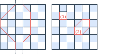
mc_cullenlandau_83 carried out Monte Carlo simulations of quantum Heisenberg chains mapped to two-dimensional Ising systems with 4-spin interactions like in Section II.2. The classical Metropolis can be employed to simulate the Ising like system only with an adapted spin flipping method. The spin flipping pattern is the major difficulty, as the mapped Ising model only allows configurations with the 4-spin plaquettes in Figure 1. Flipping an arbitrary pattern of spins will in general not lead to a transition from one allowed state to another. The plaquettes can be transformed into each other by flipping either two or four spins. As each spin is shared between two plaquettes on the grid, flipping two spins of a particular plaquette results in illegal configurations on the two adjacent plaquettes. In order to obtain an allowed state, a closed string of spins must be flipped, i.e. the first and the last flipped spin lie on the same plaquette. mc_cullenlandau_83 used two kinds of closed strings: zig-zag and local patterns shown in Figure 8. The zigzag strings are built of only vertical and diagonal steps and start at the bottom line. Lateral steps are not allowed. The flipping algorithm is restricted to the smaller pattern (1) of the local patterns because pattern (2) and all larger patterns can be constructed by merging several patterns of type (1). These restrictions were validated in a comparison with a more complicated unrestricted flipping algorithm. In this second algorithm, vertical, lateral and diagonal steps and a random starting point were allowed. The string is built up until it intersects itself and the tail is discarded to obtain a closed string. The two algorithms gave similar numerical results.
The restricted flipping algorithm is outlined in Algorithm 1. In mc_cullenlandau_83 , each zigzag pattern is constructed step by step randomly with increasing bias that ensures that the string is closed. In the implementation of this work, all possible zigzag patterns are constructed and a random uniform choice is made among them. All possible zigzag patterns are found in a brute-force search.
Appendix F Experimental details
The hyperparameter setup that was used to train the PixelCNN models is shown in Table 1. A PixelCNN architecture with residual connections and a kernel radius of as employed. On a Nvidia Tesla V100 GPU, training took for and and for . For the estimates, amples were generated which took for and for . The MCMC algorithm was implemented as described in Appendix E. After equilibration steps, Monte Carlo steps were used for the trotterized Heisenberg chain and Monte Carlo steps were used for . The Markov chain was initialized in the ground states of either model, which is a state of either only or plaquettes for the almost isotropic chain, and a state of only plaquettes for the XY chain.
| parameter | value |
|---|---|
| sampler | PixelCNN |
| depth | 6 |
| width | 64 |
| batch size | 512 |
| learning rate | 0.001 |
| steps | 10000 |
| parameters |
Appendix G Plaquette distributions
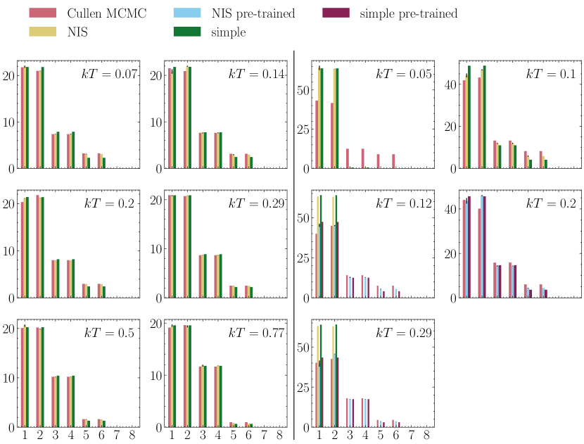
Figure 9 and Figure 10 show the plaquette distributions as obtained from different algorithms for the XY and the isotropic Heisenberg chain and the isotropic Heisenberg chain, respectively.
References
- (1) M. Newman and G. Barkema, Monte Carlo Methods in Statistical Physics. Clarendon Press, 1999.
- (2) C. Gattringer and C. Lang, Quantum Chromodynamics on the Lattice: An Introductory Presentation. Lecture Notes in Physics. Springer Berlin Heidelberg, 2009.
- (3) G. Torlai and R. G. Melko Phys. Rev. B 94 (Oct, 2016) 165134.
- (4) A. Morningstar and R. G. Melko J. Mach. Learn. Res. 18 no. 1, (Jan., 2017) 5975–5991.
- (5) F. D’Angelo and L. Böttcher Phys. Rev. Research 2 (Jun, 2020) 023266.
- (6) N. Walker, K.-M. Tam, and M. Jarrell Scientific Reports 10 no. 1, (Aug, 2020) 13047.
- (7) D. Wu, L. Wang, and P. Zhang Phys. Rev. Lett. 122 (Feb, 2019) 080602.
- (8) K. Nicoli, P. Kessel, N. Strodthoff, W. Samek, K.-R. Müller, and S. Nakajima arXiv preprint 1903.11048 (2019) , arXiv:1903.11048 [cond-mat.stat-mech].
- (9) K. A. Nicoli, S. Nakajima, N. Strodthoff, W. Samek, K.-R. Müller, and P. Kessel Phys. Rev. E 101 (Feb, 2020) 023304.
- (10) G. Carleo and M. Troyer Science 355 no. 6325, (2017) 602–606.
- (11) O. Sharir, Y. Levine, N. Wies, G. Carleo, and A. Shashua Phys. Rev. Lett. 124 (Jan, 2020) 020503.
- (12) F. Noé, S. Olsson, J. Köhler, and H. Wu Science 365 no. 6457, (2019) .
- (13) T. Vieijra, C. Casert, J. Nys, W. De Neve, J. Haegeman, J. Ryckebusch, and F. Verstraete Phys. Rev. Lett. 124 (Mar, 2020) 097201.
- (14) L. Yang, Z. Leng, G. Yu, A. Patel, W.-J. Hu, and H. Pu Phys. Rev. Research 2 (Feb, 2020) 012039.
- (15) K. Zhou, G. Endrődi, L.-G. Pang, and H. Stöcker Phys. Rev. D 100 (Jul, 2019) 011501.
- (16) J. M. Pawlowski and J. M. Urban Machine Learning: Science and Technology 1 no. 4, (Oct, 2020) 045011.
- (17) M. S. Albergo, G. Kanwar, and P. E. Shanahan Phys. Rev. D 100 (Aug, 2019) 034515.
- (18) K. A. Nicoli, C. J. Anders, L. Funcke, T. Hartung, K. Jansen, P. Kessel, S. Nakajima, and P. Stornati arXiv preprint 2007.07115 (2020) , arXiv:2007.07115 [hep-lat].
- (19) G. Kanwar, M. S. Albergo, D. Boyda, K. Cranmer, D. C. Hackett, S. Racanière, D. J. Rezende, and P. E. Shanahan Phys. Rev. Lett. 125 (Sep, 2020) 121601.
- (20) D. Boyda, G. Kanwar, S. Racanière, D. J. Rezende, M. S. Albergo, K. Cranmer, D. C. Hackett, and P. E. Shanahan arXiv preprint 2008.05456 (2020) , arXiv:2008.05456 [hep-lat].
- (21) D. Bitko, T. Rosenbaum, and G. Aeppli Physical review letters 77 no. 5, (1996) 940.
- (22) M. Kenzelmann, R. Coldea, D. Tennant, D. Visser, M. Hofmann, P. Smeibidl, and Z. Tylczynski Physical Review B 65 no. 14, (2002) 144432.
- (23) O. Breunig, M. Garst, E. Sela, B. Buldmann, P. Becker, L. Bohatỳ, R. Müller, and T. Lorenz Physical Review Letters 111 no. 18, (2013) 187202.
- (24) O. Breunig, M. Garst, A. Klümper, J. Rohrkamp, M. M. Turnbull, and T. Lorenz Science Advances 3 no. 12, (2017) .
- (25) S. Chen, L. Wang, S.-J. Gu, and Y. Wang Physical Review E 76 no. 6, (2007) 061108.
- (26) A. Osterloh, L. Amico, G. Falci, and R. Fazio Nature 416 no. 6881, (2002) 608–610.
- (27) L. F. Santos Journal of mathematical physics 50 no. 9, (2009) 095211.
- (28) H. Bethe Zeitschrift fur Physik 71 no. 3-4, (Mar., 1931) 205–226.
- (29) J. C. Bonner and M. E. Fisher Phys. Rev. 135 (Aug, 1964) A640–A658.
- (30) M. Takahashi Progress of Theoretical Physics 46 no. 2, (08, 1971) 401–415.
- (31) T. Koma Progress of Theoretical Physics 78 no. 6, (12, 1987) 1213–1218.
- (32) M. Inoue and M. Suzuki Progress of Theoretical Physics 79 no. 3, (03, 1988) 645–664.
- (33) T. D. Schultz, D. C. Mattis, and E. H. Lieb Rev. Mod. Phys. 36 (Jul, 1964) 856–871.
- (34) S. Katsura Phys. Rev. 127 (Sep, 1962) 1508–1518.
- (35) J. J. Cullen and D. P. Landau Phys. Rev. B 27 (Jan, 1983) 297–313.
- (36) M. Barma and B. S. Shastry Phys. Rev. B 18 (Oct, 1978) 3351–3359.
- (37) A. v. d. Oord, N. Kalchbrenner, O. Vinyals, L. Espeholt, A. Graves, and K. Kavukcuoglu in Proceedings of the 30th International Conference on Neural Information Processing Systems, NIPS’16, p. 4797–4805. Curran Associates Inc., Red Hook, NY, USA, 2016.
- (38) U. Wolff Computer Physics Communications 156 no. 2, (2004) 143 – 153.
- (39) A. B. Owen, Monte Carlo theory, methods and examples. 2013. https://statweb.stanford.edu/~owen/mc/. unpublished.
- (40) M. Chen, A. Radford, R. Child, J. Wu, H. Jun, P. Dhariwal, D. Luan, and I. Sutskever in Proceedings of the 37th International Conference on Machine Learning, vol. 1. 2020.
- (41) H. Trotter Proc. Amer. Math. Soc. 10 (1559) 545–551.
- (42) M. Suzuki Communications in Mathematical Physics 51 no. 2, (Jun, 1976) 183–190.
- (43) H. De Raedt and B. De Raedt Phys. Rev. A 28 (Dec, 1983) 3575–3580.