Jet tagging in the Lund plane with graph networks

Abstract

The identification of boosted heavy particles such as top quarks or vector bosons is one of the key problems arising in experimental studies at the Large Hadron Collider. In this article, we introduce LundNet, a novel jet tagging method which relies on graph neural networks and an efficient description of the radiation patterns within a jet to optimally disentangle signatures of boosted objects from background events. We apply this framework to a number of different benchmarks, showing significantly improved performance for top tagging compared to existing state-of-the-art algorithms. We study the robustness of the LundNet taggers to non-perturbative and detector effects, and show how kinematic cuts in the Lund plane can mitigate overfitting of the neural network to model-dependent contributions. Finally, we consider the computational complexity of this method and its scaling as a function of kinematic Lund plane cuts, showing an order of magnitude improvement in speed over previous graph-based taggers.

1 Introduction

As the Large Hadron Collider continues to explore proton collisions at the energy frontier, an important task to search for signals of new physics beyond the Standard Model (SM) is the identification of heavy particles at the electroweak scale, which might emerge from decays of yet unknown heavier particles.

An entity of particular interest in this quest is the jet, which is essentially defined as a collimated bunch of particles with a certain energy and direction, typically determined using a sequential recombination algorithm Salam:2009jx . One important problem is that electroweak scale particles such as vector bosons or top quarks produced from yet heavier new states can become sufficiently boosted such that their hadronic decays are reconstructed as single jets. It is therefore crucial to have efficient tools to probe the radiation patterns within jets and determine their physical origin. This topic has been the focus of much attention over the past decade, with a range of approaches being developed to extract information from a jet’s substructure Abdesselam:2010pt ; Altheimer:2012mn ; Altheimer:2013yza ; Adams:2015hiv ; Marzani:2019hun . In recent years, a new generation of tools based on deep learning models have emerged, which can achieve very high performance on specific benchmarks deOliveira:2015xxd ; Komiske:2016rsd ; Louppe:2017ipp ; Kasieczka:2017nvn ; Butter:2017cot ; Larkoski:2017jix ; Cheng:2017rdo ; Macaluso:2018tck ; Abdughani:2018wrw ; Moreno:2019bmu ; Kasieczka:2019dbj ; Qu:2019gqs ; Ren:2019xhp ; Lim:2020igi and provide some insights into what kinematic variables drive the discrimination performance Datta:2017rhs ; Datta:2017lxt ; Lim:2018toa ; Komiske:2017aww ; Komiske:2018cqr ; Chakraborty:2019imr ; Kasieczka:2020nyd ; Agarwal:2020fpt ; Chakraborty:2020yfc ; Dolan:2020qkr . A limitation of such deep learning-based methods is the difficulty to estimate their uncertainties, as well as their proneness to rely on unphysical features present in the training data to achieve their high performance, as this data is generally derived from Monte Carlo simulations of proton collisions.

In this article, we introduce a novel method to identify jets using graph networks. To this end, we represent jets through their so-called Lund plane, associating each Lund declustering with a node on the graph. Compared with other state-of-the-art tools, our new method shows improved performance, notably for processes with complicated topologies such as top decays, while requiring substantially less training time. We will also investigate the robustness of our new tagger, and show how through kinematic cuts on the Lund variables one can mitigate overfitting to the model-dependent effects of Monte Carlo simulations, reducing the reliance of the neural network on non-perturbative contributions. The code framework used to produce the results in this article are available as open-source and published material in lundnet_code .

We provide a brief review of the Lund plane for jet physics in section 2, and describe the LundNet model in section 3. Results for a range of benchmarks are described in section 4, of which a summary is given in table 1. The robustness and computational complexity of the models is explored in section 5. Finally, we offer our conclusions in section 6.

			AUC		$1/\epsilon_{B}$ at $\epsilon_{S}\!=\!0.5$	$1/\epsilon_{B}$ at $\epsilon_{S}\!=\!0.7$
	LundNet-5		0.938		609.8	70.4
	LundNet-3		0.935		500.0	61.5
$W$ tagging $p_{t}$>500 GeV	ParticleNet		0.936		480.8	60.4
	LundNet-5		0.958		12500.0	813.2
	LundNet-3		0.956		8333.3	641.0
$W$ tagging   $p_{t}$>2 TeV	ParticleNet		0.958		8333.3	626.4
	LundNet-5		0.987		5000.0	1315.8
	LundNet-3		0.982		1785.7	333.3
top tagging $p_{t}$>500 GeV	ParticleNet		0.983		2000.0	382.8
	LundNet-5		0.902		31.6	12.3
	LundNet-3		0.893		27.7	10.7
$q/g$ discrim. $p_{t}$>500 GeV	ParticleNet		0.904		34.1	12.9

Table 1: Benchmarks of several jet tagging algorithms for a range of processes. The first column gives the area under the ROC curve, and the later two show the background rejection at two different signal efficiencies, 50% and 70% respectively. In each case, larger values indicate better performance.

2 Jets in the Lund plane

The models we introduce in this article rely on the Lund plane Andersson:1988gp . This representation provides a useful mapping of the emission phase-space to a two dimensional plane representing the angle and transverse momentum of a given emission with respect to its emitter, and which is often used in discussions of resummations of large logarithms in perturbation theory or of Monte Carlo parton showers. Each emission then creates an additional triangular leaf corresponding to the phase space for further emissions. It was shown in recent work that the Lund plane provides a useful basis to achieve an efficient description of the clustering sequence of a jet, containing a rich set of information about its substructure, with notable potential for jet tagging Dreyer:2018nbf . The Lund jet plane allows for a visual representation of the clustering history of a jet. This systematic encoding of a jet’s radiation patterns can be measured experimentally Aad:2020zcn , allowing for comparisons between theoretical predictions and experimental data Lifson:2020gua and with potential for constraining general purpose Monte Carlo event generators Dasgupta:2020fwr .

Figure 1: The Lund plane representation of a jet (left) where each emission is positioned according to its $\Delta$ and $k_{t}$ coordinates, and the corresponding mapping to a binary Lund tree of tuples (right). The thick blue line represents the primary sequence of tuples $\mathcal{L}_{\text{primary}}$.

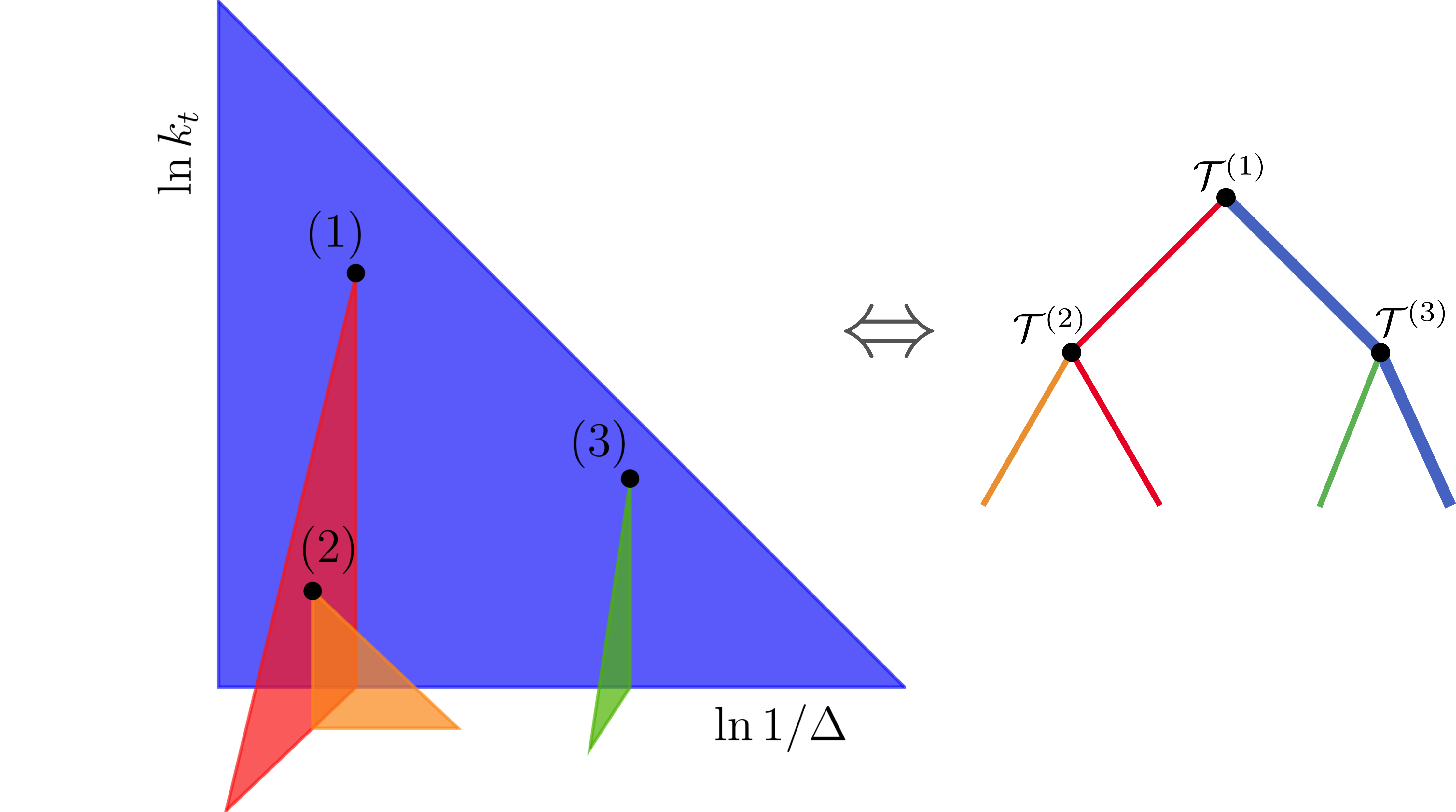
The Lund plane is obtained by first reclustering a jet’s constituents with the Cambridge/Aachen (CA) algorithm Dokshitzer:1997in ; Wobisch:1998wt , which sequentially identifies and combines the pair of particles $a$ and $b$ closest in rapidity $y$, a measure of relativistic velocity along the beam axis, and azimuthal angle $\phi$ around the same axis, i.e. minimising $\Delta^{2}=(y_{a}-y_{b})^{2}+(\phi_{a}-\phi_{b})^{2}$. We then iterate over this clustering sequence, starting from the full jet and proceeding by:

1. Declustering the current (pseudo)jet into two transverse momentum ordered pseudojets $a$ and $b$ such that $p_{t,a}>p_{t,b}$, and where we consider $b$ to be the emission of the $(a+b)$ emitter.

2. Determining a number of kinematic variables associated with the declustering step $i$, which we denote as a tuple $\mathcal{T}^{(i)}$

   $$\mathcal{T}^{(i)}=\{k_{t},\Delta,z,m,\psi\}\,.$$ (1)

   Here $k_{t}=p_{t,b}\Delta$ is the transverse momentum of emission $b$ with respect to its emitter in the limit where $p_{t,b}\ll p_{t,a}$, $\Delta$ is the previously defined rapidity-azimuth distance, $z=p_{t,b}/(p_{t,a}+p_{t,b})$ is the momentum fraction of the softer subjet $b$, $m$ is the invariant mass of the $(a+b)$ pair, and $\psi=\tan^{-1}\big{(}\tfrac{y_{b}-y_{a}}{\phi_{b}-\phi_{a}}\big{)}$ is the azimuthal angle around subjet $a$’s axis.

3. Repeating this procedure for pseudojets $a$ and $b$ if they contain more than one particle.

This procedure produces a binary Lund tree with a tuple of variables $\mathcal{T}^{(i)}$ for each node $i$ of the Lund tree, as shown in figure 1. The first two elements of the tuple provide the coordinates in the Lund plane of the corresponding splitting, and the remaining ones provide complementary kinematic information. A subset of this tree of particular significance is the primary list of tuples $\mathcal{L}_{\text{primary}}$ containing the kinematic variables of each splitting along the primary branch of the tree, i.e. following only the pseudojet with larger transverse momentum in step 3. of the algorithm above, corresponding to points on the blue primary plane in figure 1. The primary Lund sequence can be used notably for two-dimensional visual representations of the radiation patterns in a jet Dreyer:2018nbf ; Aad:2020zcn ; Andrews:2018jcm .

Figure 2: Left: Distribution of the number of Lund declusterings per jet, for different choices of $k_{t}$ cuts in the Lund plane. The dashed lines indicate the mean of each distribution. Right: Average of the number of nodes per jet as a function of the $k_{t}$ cut.

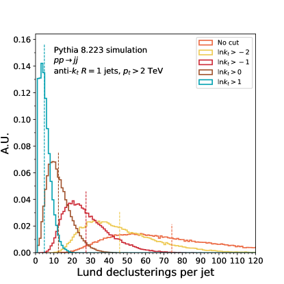
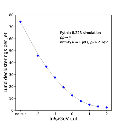
Corrections to the Lund plane originating from non-perturbative hadronisation effects affect the low $k_{t}$ region of the plane. One can therefore limit the dependence on the non-perturbative region of any model trained on Lund declusterings by removing emissions that fall below a certain transverse momentum $k_{t}$ threshold. In figure 2 (left), we show the distribution of the number of Lund declusterings per jet for several choices of $k_{t}$ cut in 2 TeV QCD jets simulated using Pythia 8.223 Sjostrand:2014zea . The mean of each distribution is indicated as a dashed line. An additional benefit of a $k_{t}$ threshold is that even for small cut values the number of nodes per jet is significantly reduced, and therefore correspondingly so the computational cost of training a machine learning model on these inputs. The right-hand side of figure 2 shows the average number of nodes per jet as a function of the $k_{t}$ cut, which decreases quadratically as the cut is increased.

3 LundNet Models

Figure 3: (a) Illustration of the EdgeConv operation on a node of the Lund tree. (b) Architecture of the EdgeConv block used in the LundNet model. (c) Architecture of the LundNet model.

The Lund plane encodes a rich set of information of the substructure and radiation patterns of a jet, therefore serving as a natural input to machine learning models for jet physics. The use of Lund planes for jet tagging was first proposed in Ref. Dreyer:2018nbf where log-likelihood and deep learning models are applied, and good performance was observed for tagging boosted electroweak bosons. However, the main focus of Ref. Dreyer:2018nbf was the primary Lund plane, which inevitably leads to some loss of information due to the omission of the secondary and tertiary splittings. In this article, we propose LundNet, a new deep learning model capable of digesting the full Lund plane. Graph neural networks are used in this model to better exploit the structural information associated with the Lund plane representation of a jet, leading to significantly improved performance on a range of jet tagging benchmarks.

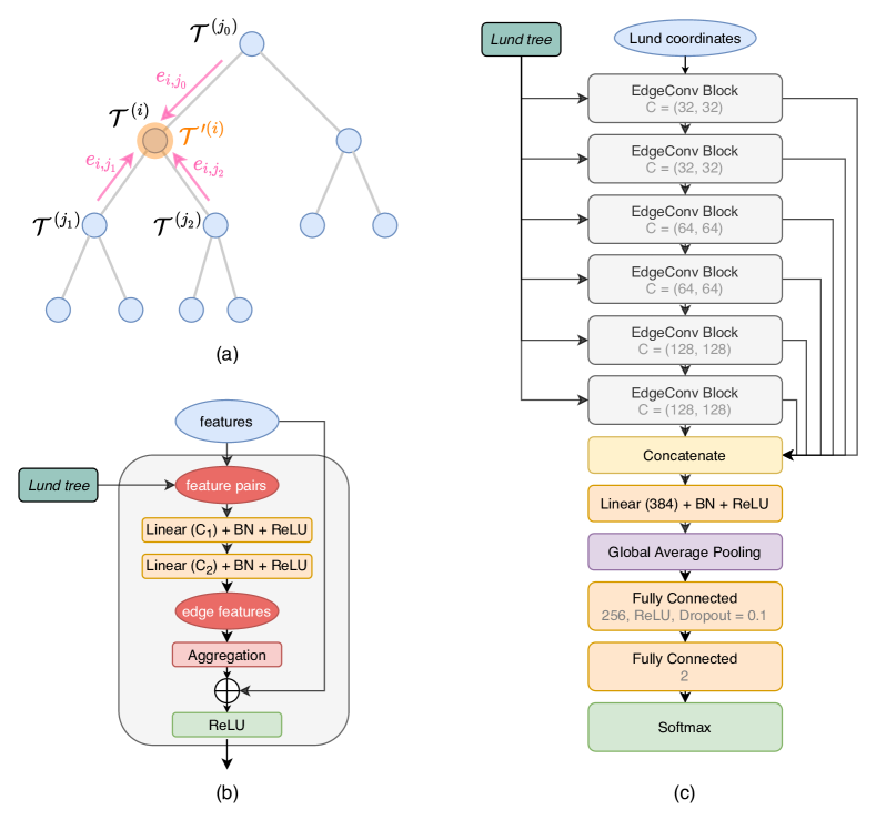
The LundNet model starts with transforming the Lund tree into a graph, where each node corresponds to a Lund declustering and carries the tuple of kinematic variables $\mathcal{T}^{(i)}$ as its input features, and bidirectional edges are formed following the structure of the Lund declustering tree. The graph network architecture is adapted from the ParticleNet Qu:2019gqs model, with the EdgeConv operation proposed in Ref. DGCNN as a core step. Figure 3(a) illustrates how EdgeConv operates for one node (the highlighted one) in the Lund tree. It consists of two steps: First, a shared multi-layer perceptron (MLP) is applied to each of its incoming edges, using features of the node pair connected by the edge as inputs, and produces a learned “edge feature”. As the Lund tree is a binary tree, there are only up to three edges for each node, which do not require a nearest-neighbour search, therefore the computational cost is much lower than for the ParticleNet model. As shown in figure 3(b), we use two layers for this shared MLP, each consisting of a linear layer followed by a batch normalization (BN) DBLP:journals/corr/IoffeS15 and a ReLU activation glorot2011deep . Then, an aggregation step is performed for the node by taking an element-wise average of the learned edge features of all the incoming edges. A shortcut connection he2016deep is also added to take the original node features into account directly, and the node feature is then updated to the new value. This operation is performed for all the nodes using the same shared MLPs, therefore updating all the node features but keeping the graph structure unchanged.

The architecture of the LundNet model is shown in figure 3(c). We stack six such EdgeConv blocks to form a deep graph network. The number of channels of the MLPs are $(32,32)$, $(32,32)$, $(64,64)$, $(64,64)$, $(128,128)$ and $(128,128)$ for the six EdgeConv blocks, respectively. Outputs from these EdgeConv blocks are concatenated per node and further processed by another MLP with 384 channels to better aggregate features learned at different stages. A global average pooling is applied afterwards to read out information from all nodes in the graph. This is followed by a fully connected layer with 256 units and a dropout layer with a drop probability of 0.1, before the final classification output.

The LundNet model uses the Lund kinematic variables defined in equation (1) as the input node features. Two variants of the LundNet models are investigated in this article. The first one uses all five Lund variables,

$$(\ln k_{t},\ln\Delta,\ln z,\ln m,\psi)\,$$ (2)

as input features to extract as much information as possible from the Lund plane to maximize the jet tagging performance and is referred to as LundNet-5. The second one uses only three Lund variables,

$$(\ln k_{t},\ln\Delta,\ln z)\,$$ (3)

and is referred to as LundNet-3. The removal of the $\ln m$ and $\psi$ variables significantly increases the resilience of the model to non-perturbative effects at only a small cost of the performance, as will be discussed in Section 5.

We implement the LundNet model with the Deep Graph Library 0.4.3 wang2019dgl using the PyTorch 1.7 NEURIPS2019_9015 backend. The training is performed on a Nvidia GTX 1080 Ti graphics card with a minibatch size of 256. The Adam optimizer DBLP:journals/corr/KingmaB14 is used to minimize the cross entropy loss. The training is performed for 30 epochs, with an initial learning rate of 0.001, and subsequently lowered by a factor of 10 after the 10th and the 20th epochs. A snapshot of the model is saved at the end of each epoch, and the model snapshot showing the best accuracy on the validation dataset is selected for the final evaluation.

4 Jet tagging in the Lund plane

Let us now turn to a detailed evaluation of our models for the identification of several hallmark signals at the LHC. We will look at four different benchmarks: the tagging of boosted electroweak $W$ for two different transverse momentum cuts, the tagging of top quarks, and the discrimination between quark and gluon jets. The data samples consist in each benchmark of 1.2m signal and background jets simulated through the corresponding process with Pythia 8.223 Sjostrand:2014zea , with an equal split between signal and background events. Events are generated at hadron-level with underlying event turned on, but without including detector effects or the presence of additional pile-up collisions. A subset of 100k jets each are used as validation and test data, with the same number of signal and background events in both samples. All data sets are taken from Ref. Carrazza:2019efs ; groomRL_data . Jets are clustered using the anti-$k_{t}$ algorithm Cacciari:2008gp ; Cacciari:2011ma with a radius $R=1.0$ using FastJet 3.3.2, and are required to pass a selection cut, with transverse momentum $p_{t}>500$ GeV or $p_{t}>2$ TeV as indicated, and rapidity $|y|<2.5$. In each event, only the two jets with the highest transverse momentum are considered, and are saved as training data if they pass the selection cuts. A summary of these benchmarks is given in table 1.

4.1 $W$ tagging

Figure 4: Background rejection $1/\epsilon_{\text{QCD}}$ versus signal efficiency $\epsilon_{W}$ for $W$ jet tagging with transverse momentum $p_{t}>500$ GeV.

We start by considering the identification of hadronically decaying $W$ bosons, one of the key objects commonly appearing in high energy proton collisions. The signal data is obtained from 600k jets passing the selection cuts and simulated using the $pp\rightarrow WW$ process, where the $W$ bosons are decayed hadronically. The background consists of the same number of QCD jets simulated through a sample of $pp\rightarrow jj$ events. Training of the neural network weights for every model is performed using 500k of the $W$ and background samples each. At the end of each epoch, the performance is monitored on a separate validation sample consisting of 100k jets. The final performance of each model is then evaluated using a further independent sample of 100k jets with an equal number of signal and background events.

In fig. 4 we show for each model the background rejection $1/\epsilon_{\mathrm{QCD}}$ against the signal efficiency $\epsilon_{W}$ for $W$ bosons, for jets passing a transverse momentum cut of $p_{t}>500$ GeV. Better performance translates to curves that achieve a higher background rejection for a given signal efficiency, i.e. which are closer to the top right corner of the figure. We compare the LundNet-3 and LundNet-5 models with three recent benchmarks: the ParticleNet model introduced in Qu:2019gqs , the RecNN model from Louppe:2017ipp and the Lund+LSTM model from the original Lund plane paper Dreyer:2018nbf , which uses an LSTM network on the primary Lund sequence. Both the RecNN and the Lund+LSTM models, while superior to heuristic substructure algorithms, are vastly outperformed by all of the graph based methods considered. The LundNet-3 model is able to achieve about the same signal purity as ParticleNet, but can be trained in substantially less time, as will be discussed in more detail in section 5.3, and takes only a small 3-dimensional input for each declustering node in the Lund plane. By including more kinematic information, the LundNet-5 model is able to provide a slightly higher performance, but as we will see in section 5, this comes at the price of being less robust to non-perturbative effects than its lower-dimensional counterpart.

Figure 5: Background rejection $1/\epsilon_{\text{QCD}}$ versus signal efficiency $\epsilon_{W}$ for $W$ jet tagging with transverse momentum $p_{t}>2$ TeV.

In figure 5, we show the same process but with a transverse momentum selection cut of $p_{t}>2$ TeV for the jets. Here we can observe roughly the same qualitative behaviour as at lower transverse momentum, but with the LundNet-5 model now clearly outperforming the remaining taggers even at high signal efficiencies. At higher transverse momentum, the peak in the Lund plane associated with the $W$ splitting, and the corresponding depletion associated with the colour-singlet nature of the $W$, become more distinguishable. The Lund+LSTM model, which relies purely on the primary Lund sequence, also shows a strong performance, although it is still lags significantly behind all the graph-based approaches.

4.2 Top tagging

Figure 6: Background rejection $1/\epsilon_{\text{QCD}}$ versus signal efficiency $\epsilon_{\text{Top}}$ for top jet tagging with transverse momentum $p_{t}>500$ GeV.

We now turn to the identification of jets originating from top quark decays. Top quarks are of particular interest at the LHC, interacting strongly with the Higgs boson and providing a valuable avenue in searches for new physics, as well as being the only quarks to decay before hadronising. Here the signal data is obtained from the $pp\rightarrow t\bar{t}$ process in Pythia 8.223, where the top quarks decay to hadrons and the jets are required to pass a 500 GeV transverse momentum cut. The background QCD jets are identical to the ones used in figure 4. Each model is again trained using 500k signal and 500k background jets, with further validation and testing samples that are both one tenth the size of the training data.

In fig. 6, we show the QCD background rejection as a function of the top efficiency. In this case, the Lund+LSTM model does not perform as well as RecNN. This is to be expected, as it was designed for one or two-pronged jet identification and uses only information from the primary Lund declustering sequence. It therefore contains information about the structure of only one of the initial decay products of the original top quark, limiting the performance that can be achieved without input from secondary planes. It is however interesting to see that in this process with more complex topology, the LundNet-5 model provides a substantial performance gain over existing state-of-the-art methods such as ParticleNet. This is due to the nature of its input, which contains already high-level kinematic information about the radiation patterns of the jet, making it much simpler for the neural network to learn how to distinguish signals with more involved signatures. Thus the LundNet-3 model achieves almost the same signal purity as the ParticleNet algorithm, despite having as input only a reduced 3-tuple of kinematic variables per node and taking about an order of magnitude less time to train. Interestingly, the performance gap between the two LundNet taggers is entirely due to the addition of the subjet mass and azimuthal angle $\psi$ to the input features of each declustering for the LundNet-5 model.

4.3 Quark/Gluon discrimination

Figure 7: Background rejection $1/\epsilon_{\text{Gluon}}$ versus signal efficiency $\epsilon_{\text{Quark}}$ for quark/gluon discrimination between $R=0.4$ anti-$k_{t}$ jets with transverse momentum $p_{t}>500$ GeV.

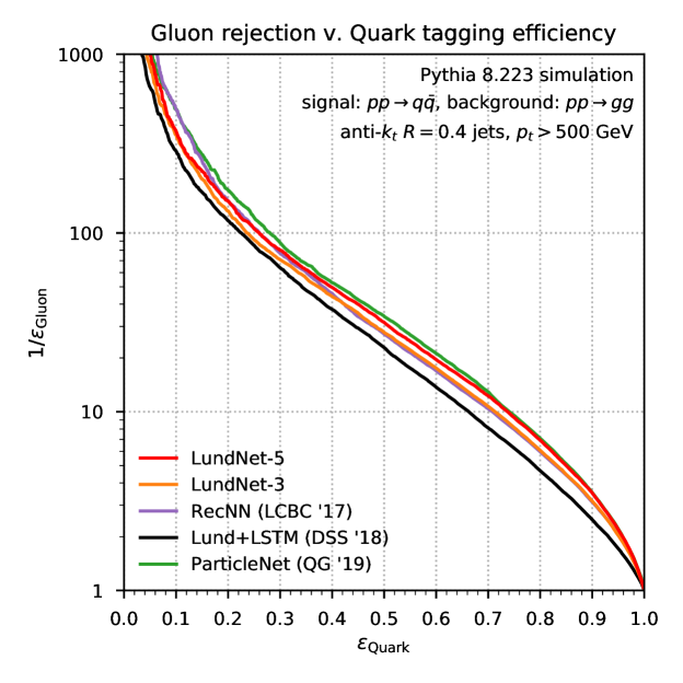
Our final benchmark considers the discrimination between quark and gluon initiated jets, a core challenge in collider physics which has seen much research in recent years Gallicchio:2011xq ; Larkoski:2013eya ; Larkoski:2014pca ; Bhattacherjee:2015psa ; Komiske:2016rsd ; Frye:2017yrw ; Metodiev:2018ftz ; Larkoski:2019nwj . For this study, we consider a signal sample of 500k quark-initiated jets obtained through the $q\bar{q}\rightarrow q\bar{q}$ process in Pythia 8.223, while the background is obtained from $gg\rightarrow gg$ events. The jets are clustered with an anti-$k_{t}$ algorithm with radius $R=0.4$ and are again required to pass a transverse momentum $p_{t}>500$ GeV and rapidity $|y|<2.5$ selection cut.

The gluon-jet rejection as a function of the quark-jet efficiency is shown in figure 7. In this case there is not as large a hierarchy between models, with the Lund+LSTM model performing somewhat below the competing approaches. ParticleNet has a slight edge over the other algorithms at small quark efficiencies, but is indistinguishable from the LundNet-5 tagger at high efficiency. The LundNet-3 and RecNN models show similar performance at high efficiency, with RecNN providing slightly higher gluon rejection at lower quark efficiencies.

5 Robustness study

We will now investigate the robustness of the different models we considered in our benchmarks. To this end we will consider three axes: their resilience to non-perturbative effects, their resilience to detector effects, and the complexity and computational cost of each tagger.

5.1 Non-perturbative effects

Figure 8: Performance $\tfrac{\epsilon_{W}}{\sqrt{\epsilon_{\text{QCD}}}}$ versus resilience to non-perturbative effects.

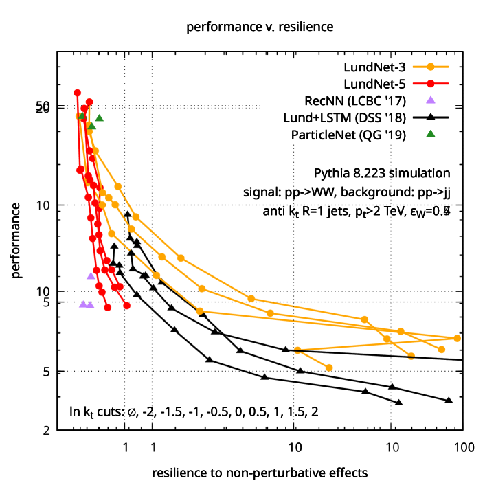
Beyond its raw performance, it is important for practical applications that a tagger be relatively robust to model-dependent non-perturbative effects. To carry out studies of sensitivity to non-perturbative effects, we compare performance between a data sample of both 50k signal and background jets produced at parton level, and a sample obtained with hadronisation and underlying event models turned on in the event generator. The same model, trained on hadron-level data, is evaluated on both samples for the comparison. For this study, we use the same 2 TeV $W$ jet sample as was used in section 4.1 as well as the corresponding models shown in figure 5, which are now used to label jets from both parton and hadron-level data.

Figure 9: Background rejection as a function of $W$ tagging efficiency. Dotted lines indicate a $W$ tagger applied on parton-level data.

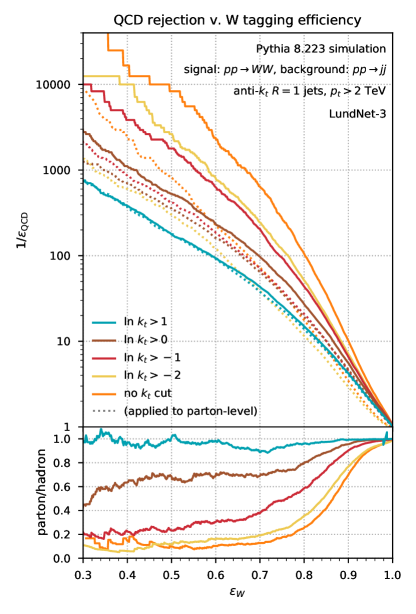
Figure 8 shows the robustness of the tagger in conjunction with its performance. This robustness is measured through the resilience $\zeta_{\text{NP}}$ Bendavid:2018nar , calculated using both the efficiency on the hadron-level sample, $\epsilon$, and that on the parton-level sample, $\epsilon^{\prime}$

$$\zeta_{\text{NP}}=\left(\frac{\Delta\epsilon_{W}^{2}}{\langle\epsilon\rangle^{2}_{W}}+\frac{\Delta\epsilon_{\mathrm{QCD}}^{2}}{\langle\epsilon\rangle^{2}_{\mathrm{QCD}}}\right)^{-1/2}\,,$$ (4)

where $\Delta\epsilon=\epsilon-\epsilon^{\prime}$ and $\langle\epsilon\rangle=1/2\left(\epsilon+\epsilon^{\prime}\right)$. The efficiencies are obtained with a fixed cut corresponding to a signal efficiency $\epsilon_{W}=70\%$ on the hadron-level sample. The curves in figure 8 are obtained by increasing a transverse momentum cut on the $k_{t}$ variable of the Lund plane, progressively removing declustering nodes that fall below the cut. Each curve starts on the upper left of figure 8, with a model trained without any cuts on the Lund plane, and ends in the lower right part of the figure with a model trained with a transverse momentum cut $\ln k_{t}/\text{GeV}>2$ that has higher resilience but lower performance due to the removal of parts of the Lund tree. We can observe that despite their good performance, the ParticleNet and RecNN models have very little resilience to non-perturbative effects, and have no handles through which such robustness can be consistently imposed. Somewhat surprisingly, the LundNet-5 also offers relatively poor robustness to non-perturbative effects. This is due to its higher dimensional input state, which allows the neural network to extrapolate some information on emissions in the non-perturbative regime despite the presence of a transverse momentum cut. In particular, the mass variable present in the input of the LundNet-5 model contains information about soft wide-angle emissions further down the clustering tree, as these will increase the mass of the subjet even if they are then removed after failing a $k_{t}$ cut. In contrast, the LundNet-3 model becomes very resilient to non-perturbative effects as the transverse momentum cut is increased, outperforming the Lund+LSTM model by a factor two for the same resilience value.

In figure 9 (left), we show the ROC curve for each model trained on the hadron-level $W$ data, with the ROC curve obtained on the parton-level data shown as a dotted line. The lower panel provides the ratio between the parton-level ROC curve and the hadron-level one. The right-hand side of figure 9 gives the ROC curve of the LundNet-3 models obtained for several choices of the $\ln k_{t}$ transverse momentum cut applied on the Lund tree. Here we can observe the improved resilience as the $k_{t}$ cut is increased, with the $\ln k_{t}/\text{GeV}>1$ model providing almost the same performance at parton and hadron level, albeit at the cost of a factor 20 in background rejection when compared to the unconstrained model.

5.2 Detector effects

Figure 10: Performance $\tfrac{\epsilon_{W}}{\sqrt{\epsilon_{\text{QCD}}}}$ versus resilience to detector effects.

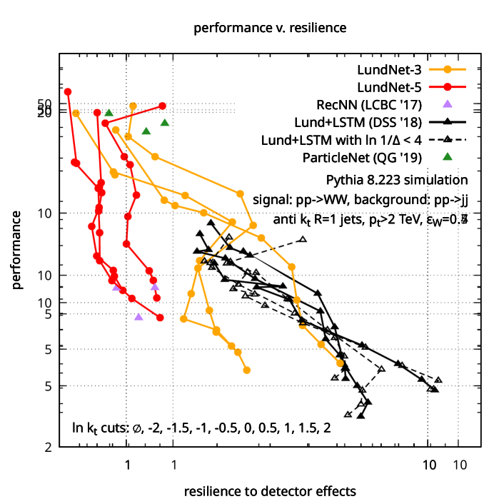
Let us now turn to the impact of detector effects on the model robustness. To this end, we create a sample of 100k 2 TeV $W$ and QCD jets using Pythia 8.223, including fast detector simulation with Delphes v3.4.1 using the delphes_card_CMS_NoFastJet.tcl card to simulate both detector effects and particle flow reconstruction deFavereau:2013fsa . The effects of detector granularity are then partially mitigated by applying a subjet-particle rescaling algorithm Dreyer:2018nbf ; Son:2012mb , where the Delphes particle-flow objects in a jet are reclustered into subjets using a CA algorithm with $R_{h}=0.12$ and rescaling the particle flow charged-particle and photons by a factor

$$f=\frac{\sum_{i\in\text{subjet}}p_{t,i}}{\sum_{i\in\text{subjet}(h^{\pm},\gamma)}p_{t,i}}.$$ (5)

before discarding neutral hadron candidates. The resulting particles of all subjets are then reclustered into a single jet on which the Lund tree can be measured.

Figure 11: Background rejection as a function of $W$ tagging efficiency. Dotted lines indicate a $W$ tagger applied on detector-level data.

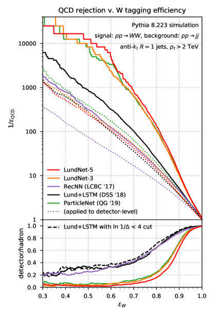
Applying the 2 TeV $W$ taggers trained in section 4.1 on this sample, we can now compute an index of resilience to detector effects $\zeta_{\text{D}}$ in the same way as was done for non-perturbative effects, but taking now $\epsilon^{\prime}$ in equation (4) to be the detector-level efficiency. We show in figure 10 the resilience as a function of performance $\epsilon_{W}/\sqrt{\epsilon_{\text{QCD}}}$ for a signal efficiency of $\epsilon_{W}=70\%$ on the hadron-level data. One can observe here that while for high performance, good resilience can be achieved, a transverse momentum cut in the Lund plane does not result models that are particularly insensitive to detector effects. Adding a further Lund-plane angular cut $\ln 1/\Delta<4$ to remove unmitigated effects due to electromagnetic calorimeter granularity did not provide any noticeable improvement, as is shown in dashed lines in the figure for the Lund+LSTM model.

The limitations in achieving higher resilience values for any of the considered models are due to the consistently enhanced performance of taggers at hadron-level. We show the ROC curves for each model in figure 11 (left), with the dotted lines showing the hadron-level model applied on detector-level data. Here one can note the performance of the Lund+LSTM model on the detector-level sample, achieving performance quite close to the LundNet and ParticleNet models. The LundNet-5 model in particular, is performing slightly worse than LundNet-3 when applied on the detector-level sample, despite having a substantial edge over it on the hadron-level data that both were trained on. The lower panel gives the ratio between both curves, with the background rejection ratio of the Lund+LSTM tagger with an angular cut $\ln 1/\Delta<4$ shown in dashed lines. In the right-hand side of figure 11, one can see the ROC curve of the LundNet-3 model trained for increasing $k_{t}$ cuts, showing somewhat improved robustness at larger cut values.

5.3 Complexity of models

An important quality for a deep learning-based jet tagger is the simplicity of the model, and the speed of its training and inference on new samples. To quantify these considerations we measure three different metrics for the models:

• the number of trainable parameters of the model,

• the training time of each model per data sample and per epoch, which provides a measure of the time needed to train a full tagger on a given data set,

• and finally the inference time per sample of the trained model on new data points, which provides a measure of how efficiently an existing model can be deployed to label a given sample of jets.

		Number of		Training time	Inference time
		parameters		[ms/sample/epoch]	[ms/sample]
LundNet		395k		0.472	0.117
ParticleNet		369k		3.488	1.036
Lund+LSTM		67k		0.424	0.131

Table 2: Summary for each model of the number of parameters, training time per sample and epoch, and inference time per sample. The time is measured in milliseconds as obtained when running the models on an Nvidia GTX 1080 Ti card.

We evaluate the training time on the 2 TeV $W$ and QCD training sample used previously in section 4.1, and the inference time on the corresponding test data of 100k jets. The results are shown in table 2 for the graph-based models and the LSTM tagger. As LundNet-3 and LundNet-5 only differs in the dimension of the input features, the number of parameters and the computational cost are essentially the same, therefore we do not distinguish between them in this section and provide numbers derived from the LundNet-3 tagger. The Lund+LSTM model has a much simpler architecture, resulting in only 67k trainable parameters, significantly less than any of the graph-based models. It is however not substantially faster than these larger models, and even underperforms the LundNet models in inference time. The relatively long training time is partly due to the smaller learning rate used when training the LSTM network, and the smaller number of epochs needed for the Lund+LSTM model to converge. Due to its increased number of EdgeConv blocks, the LundNet model has 26k more parameters than ParticleNet. However, the direct use of the Lund tree as the graph structure removes the need for a costly nearest-neighbour search and also significantly reduces the number of edges for each node, therefore increasing both the training and inference speed by almost an order of magnitude. This is compounded by the fact that due to their higher-level kinematic inputs, the LundNet models take significantly less epochs to converge to a good solution.

Figure 12: Inference time per jet of the LundNet model as a function of the mean number of Lund declusterings per 2 TeV QCD jet. Each circle corresponds to a separate LundNet model trained for a different $k_{t}$ cut, as indicated in the figure text.

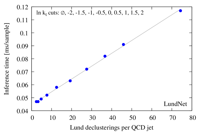
An interesting side-effect of the $k_{t}$ cut applied in the Lund plane to improve the robustness of the model as described in previous sections is that it also reduces the number of nodes present in the graph. As such, both the training and the inference time of the model are expected to be reduced as the transverse momentum cut is increased and more nodes are removed from the input graph. To demonstrate this we show in figure 12 the inference time per sample as a function of the average number of Lund declusterings per QCD jet, obtained through models trained with different Lund plane $k_{t}$ cuts, each of which is shown as blue circle. As expected, the inference time scales linearly with the number of nodes in the graph, such that computing time increases quadratically as the $\ln k_{t}$ cut is reduced.

6 Conclusions

In this article, we have introduced LundNet, a novel algorithm used to detect signals at the LHC. We showed that this method provides substantial improvements over existing methods on the identification of key benchmark processes, as well as in training speed and robustness to non-perturbative effects.

The LundNet model combines the power of graph convolutional networks with an efficient representation of the radiation patterns within a jet to optimally extract information from its substructure. Jets are represented through a Lund tree constructed from the CA clustering tree of each jet. Each node of the Lund tree contains a tuple of kinematic information for the corresponding pairwise splitting, used as input to the graph network. By using the clustering tree structure to aggregate information in the graph convolution, the weights of the LundNet model can be trained ten times faster than previous graph-based methods such as ParticleNet, with a similar gain on the inference time when applying the trained model to identify new jets.

We introduced two taggers, LundNet-3 and LundNet-5 which rely on a three- and five-dimensional emission feature space respectively. The LundNet-5 tagger outperforms current state-of-the-art methods on several pivotal jet tagging benchmarks, most notably for the identification of jets originating from top decays, while the lower-dimensional LundNet-3 tagger matches the performance of current jet taggers despite its reduced kinematic input size.

We provided a concrete study of its resilience to model-dependent non-perturbative and detector effects. Through the use of an appropriate transverse momentum cut in the Lund plane, we showed how one can establish an algorithm that retains high performance while maintaining a handle on robustness. Due to its limited kinematic input, the LundNet-3 tagger is best positioned to provide jet identification that is relatively insensitive to non-perturbative effects and detector smearing, while substantially outperforming previous methods based on the primary Lund plane.

These results offer a concrete avenue to implementing effective machine-learning based taggers that can be robust to model-dependent effects present in the training data, a key feature for real-life applications of artificial intelligence at the LHC. In this context, the work presented in this article provides a key step towards a new generation of efficient, robust and tractable jet substructure tools for LHC physics.

References

- (1) G. P. Salam, Towards Jetography, Eur. Phys. J. C 67 (2010) 637–686, [arXiv:0906.1833].
- (2) A. Abdesselam et al., Boosted Objects: A Probe of Beyond the Standard Model Physics, Eur. Phys. J. C 71 (2011) 1661, [arXiv:1012.5412].
- (3) A. Altheimer et al., Jet Substructure at the Tevatron and LHC: New results, new tools, new benchmarks, J. Phys. G 39 (2012) 063001, [arXiv:1201.0008].
- (4) A. Altheimer et al., Boosted Objects and Jet Substructure at the LHC. Report of BOOST2012, held at IFIC Valencia, 23rd-27th of July 2012, Eur. Phys. J. C 74 (2014), no. 3 2792, [arXiv:1311.2708].
- (5) D. Adams et al., Towards an Understanding of the Correlations in Jet Substructure, Eur. Phys. J. C 75 (2015), no. 9 409, [arXiv:1504.00679].
- (6) S. Marzani, G. Soyez, and M. Spannowsky, Looking inside jets: an introduction to jet substructure and boosted-object phenomenology, vol. 958. Springer, 2019.
- (7) L. de Oliveira, M. Kagan, L. Mackey, B. Nachman, and A. Schwartzman, Jet-images — deep learning edition, JHEP 07 (2016) 069, [arXiv:1511.05190].
- (8) P. T. Komiske, E. M. Metodiev, and M. D. Schwartz, Deep learning in color: towards automated quark/gluon jet discrimination, JHEP 01 (2017) 110, [arXiv:1612.01551].
- (9) G. Louppe, K. Cho, C. Becot, and K. Cranmer, QCD-Aware Recursive Neural Networks for Jet Physics, JHEP 01 (2019) 057, [arXiv:1702.00748].
- (10) G. Kasieczka, T. Plehn, M. Russell, and T. Schell, Deep-learning Top Taggers or The End of QCD?, JHEP 05 (2017) 006, [arXiv:1701.08784].
- (11) A. Butter, G. Kasieczka, T. Plehn, and M. Russell, Deep-learned Top Tagging with a Lorentz Layer, SciPost Phys. 5 (2018), no. 3 028, [arXiv:1707.08966].
- (12) A. J. Larkoski, I. Moult, and B. Nachman, Jet Substructure at the Large Hadron Collider: A Review of Recent Advances in Theory and Machine Learning, arXiv:1709.04464.
- (13) T. Cheng, Recursive Neural Networks in Quark/Gluon Tagging, Comput. Softw. Big Sci. 2 (2018), no. 1 3, [arXiv:1711.02633].
- (14) S. Macaluso and D. Shih, Pulling Out All the Tops with Computer Vision and Deep Learning, JHEP 10 (2018) 121, [arXiv:1803.00107].
- (15) M. Abdughani, J. Ren, L. Wu, and J. M. Yang, Probing stop pair production at the LHC with graph neural networks, JHEP 08 (2019) 055, [arXiv:1807.09088].
- (16) E. A. Moreno, O. Cerri, J. M. Duarte, H. B. Newman, T. Q. Nguyen, A. Periwal, M. Pierini, A. Serikova, M. Spiropulu, and J.-R. Vlimant, JEDI-net: a jet identification algorithm based on interaction networks, Eur. Phys. J. C 80 (2020), no. 1 58, [arXiv:1908.05318].
- (17) A. Butter et al., The Machine Learning Landscape of Top Taggers, SciPost Phys. 7 (2019) 014, [arXiv:1902.09914].
- (18) H. Qu and L. Gouskos, ParticleNet: Jet Tagging via Particle Clouds, Phys. Rev. D 101 (2020), no. 5 056019, [arXiv:1902.08570].
- (19) J. Ren, L. Wu, and J. M. Yang, Unveiling CP property of top-Higgs coupling with graph neural networks at the LHC, Phys. Lett. B 802 (2020) 135198, [arXiv:1901.05627].
- (20) S. H. Lim and M. M. Nojiri, Morphology for Jet Classification, arXiv:2010.13469.
- (21) K. Datta and A. Larkoski, How Much Information is in a Jet?, JHEP 06 (2017) 073, [arXiv:1704.08249].
- (22) K. Datta and A. J. Larkoski, Novel Jet Observables from Machine Learning, JHEP 03 (2018) 086, [arXiv:1710.01305].
- (23) S. H. Lim and M. M. Nojiri, Spectral Analysis of Jet Substructure with Neural Networks: Boosted Higgs Case, JHEP 10 (2018) 181, [arXiv:1807.03312].
- (24) P. T. Komiske, E. M. Metodiev, and J. Thaler, Energy flow polynomials: A complete linear basis for jet substructure, JHEP 04 (2018) 013, [arXiv:1712.07124].
- (25) P. T. Komiske, E. M. Metodiev, and J. Thaler, Energy Flow Networks: Deep Sets for Particle Jets, JHEP 01 (2019) 121, [arXiv:1810.05165].
- (26) A. Chakraborty, S. H. Lim, and M. M. Nojiri, Interpretable deep learning for two-prong jet classification with jet spectra, JHEP 19 (2020) 135, [arXiv:1904.02092].
- (27) G. Kasieczka, S. Marzani, G. Soyez, and G. Stagnitto, Towards Machine Learning Analytics for Jet Substructure, JHEP 09 (2020) 195, [arXiv:2007.04319].
- (28) G. Agarwal, L. Hay, I. Iashvili, B. Mannix, C. McLean, M. Morris, S. Rappoccio, and U. Schubert, Explainable AI for ML jet taggers using expert variables and layerwise relevance propagation, arXiv:2011.13466.
- (29) A. Chakraborty, S. H. Lim, M. M. Nojiri, and M. Takeuchi, Neural Network-based Top Tagger with Two-Point Energy Correlations and Geometry of Soft Emissions, JHEP 20 (2020) 111, [arXiv:2003.11787].
- (30) M. J. Dolan and A. Ore, Equivariant Energy Flow Networks for Jet Tagging, arXiv:2012.00964.
- (31) F. A. Dreyer and H. Qu, LundNet v1.0.0, Jan., 2021.
- (32) B. Andersson, G. Gustafson, L. Lonnblad, and U. Pettersson, Coherence Effects in Deep Inelastic Scattering, Z. Phys. C43 (1989) 625.
- (33) F. A. Dreyer, G. P. Salam, and G. Soyez, The Lund Jet Plane, JHEP 12 (2018) 064, [arXiv:1807.04758].
- (34) ATLAS Collaboration, G. Aad et al., Measurement of the Lund Jet Plane Using Charged Particles in 13 TeV Proton-Proton Collisions with the ATLAS Detector, Phys. Rev. Lett. 124 (2020), no. 22 222002, [arXiv:2004.03540].
- (35) A. Lifson, G. P. Salam, and G. Soyez, Calculating the primary Lund Jet Plane density, JHEP 10 (2020) 170, [arXiv:2007.06578].
- (36) M. Dasgupta, F. A. Dreyer, K. Hamilton, P. F. Monni, G. P. Salam, and G. Soyez, Parton showers beyond leading logarithmic accuracy, Phys. Rev. Lett. 125 (2020), no. 5 052002, [arXiv:2002.11114].
- (37) Y. L. Dokshitzer, G. D. Leder, S. Moretti, and B. R. Webber, Better jet clustering algorithms, JHEP 08 (1997) 001, [hep-ph/9707323].
- (38) M. Wobisch and T. Wengler, Hadronization corrections to jet cross-sections in deep inelastic scattering, in Monte Carlo generators for HERA physics. Proceedings, Workshop, Hamburg, Germany, 1998-1999, pp. 270–279, 1998. hep-ph/9907280.
- (39) H. A. Andrews et al., Novel tools and observables for jet physics in heavy-ion collisions, arXiv:1808.03689.
- (40) T. Sjöstrand, S. Ask, J. R. Christiansen, R. Corke, N. Desai, P. Ilten, S. Mrenna, S. Prestel, C. O. Rasmussen, and P. Z. Skands, An Introduction to PYTHIA 8.2, Comput. Phys. Commun. 191 (2015) 159–177, [arXiv:1410.3012].
- (41) Y. Wang, Y. Sun, Z. Liu, S. E. Sarma, M. M. Bronstein, and J. M. Solomon, Dynamic graph cnn for learning on point clouds, ACM Trans. Graph. 38 (Oct., 2019) 146.
- (42) S. Ioffe and C. Szegedy, Batch normalization: Accelerating deep network training by reducing internal covariate shift, in Proceedings of the 32nd International Conference on Machine Learning, vol. 37, (Lille, France), pp. 448–456, PMLR, 07–09 Jul, 2015.
- (43) X. Glorot, A. Bordes, and Y. Bengio, Deep sparse rectifier neural networks, in Proceedings of the Fourteenth International Conference on Artificial Intelligence and Statistics, vol. 15, (Fort Lauderdale, FL, USA), pp. 315–323, PMLR, 11–13 Apr, 2011.
- (44) K. He, X. Zhang, S. Ren, and J. Sun, Deep residual learning for image recognition, in 2016 IEEE Conference on Computer Vision and Pattern Recognition (CVPR), (Las Vegas, NV, USA), pp. 770–778, IEEE, 2016.
- (45) M. Wang, D. Zheng, Z. Ye, Q. Gan, M. Li, X. Song, J. Zhou, C. Ma, L. Yu, Y. Gai, T. Xiao, T. He, G. Karypis, J. Li, and Z. Zhang, Deep graph library: A graph-centric, highly-performant package for graph neural networks, arXiv preprint arXiv:1909.01315 (2019).
- (46) A. Paszke, S. Gross, F. Massa, A. Lerer, J. Bradbury, G. Chanan, T. Killeen, Z. Lin, N. Gimelshein, L. Antiga, A. Desmaison, A. Kopf, E. Yang, Z. DeVito, M. Raison, A. Tejani, S. Chilamkurthy, B. Steiner, L. Fang, J. Bai, and S. Chintala, Pytorch: An imperative style, high-performance deep learning library, in Advances in Neural Information Processing Systems 32 (H. Wallach, H. Larochelle, A. Beygelzimer, F. d'Alché-Buc, E. Fox, and R. Garnett, eds.), pp. 8024–8035. Curran Associates, Inc., 2019.
- (47) D. P. Kingma and J. Ba, Adam: A method for stochastic optimization, CoRR abs/1412.6980 (2014) [arXiv:1412.6980].
- (48) S. Carrazza and F. A. Dreyer, Jet grooming through reinforcement learning, Phys. Rev. D 100 (2019), no. 1 014014, [arXiv:1903.09644].
- (49) S. Carrazza and F. A. Dreyer, JetsGame/data v1.0.0, Mar., 2019. This repository is git-lfs.
- (50) M. Cacciari, G. P. Salam, and G. Soyez, The Anti-k(t) jet clustering algorithm, JHEP 04 (2008) 063, [arXiv:0802.1189].
- (51) M. Cacciari, G. P. Salam, and G. Soyez, FastJet User Manual, Eur. Phys. J. C72 (2012) 1896, [arXiv:1111.6097].
- (52) J. Gallicchio and M. D. Schwartz, Quark and Gluon Tagging at the LHC, Phys. Rev. Lett. 107 (2011) 172001, [arXiv:1106.3076].
- (53) A. J. Larkoski, G. P. Salam, and J. Thaler, Energy Correlation Functions for Jet Substructure, JHEP 06 (2013) 108, [arXiv:1305.0007].
- (54) A. J. Larkoski, J. Thaler, and W. J. Waalewijn, Gaining (Mutual) Information about Quark/Gluon Discrimination, JHEP 11 (2014) 129, [arXiv:1408.3122].
- (55) B. Bhattacherjee, S. Mukhopadhyay, M. M. Nojiri, Y. Sakaki, and B. R. Webber, Associated jet and subjet rates in light-quark and gluon jet discrimination, JHEP 04 (2015) 131, [arXiv:1501.04794].
- (56) C. Frye, A. J. Larkoski, J. Thaler, and K. Zhou, Casimir Meets Poisson: Improved Quark/Gluon Discrimination with Counting Observables, JHEP 09 (2017) 083, [arXiv:1704.06266].
- (57) E. M. Metodiev and J. Thaler, Jet Topics: Disentangling Quarks and Gluons at Colliders, Phys. Rev. Lett. 120 (2018), no. 24 241602, [arXiv:1802.00008].
- (58) A. J. Larkoski and E. M. Metodiev, A Theory of Quark vs. Gluon Discrimination, JHEP 10 (2019) 014, [arXiv:1906.01639].
- (59) J. R. Andersen et al., Les Houches 2017: Physics at TeV Colliders Standard Model Working Group Report, 2018. arXiv:1803.07977.
- (60) DELPHES 3 Collaboration, J. de Favereau, C. Delaere, P. Demin, A. Giammanco, V. Lemaître, A. Mertens, and M. Selvaggi, DELPHES 3, A modular framework for fast simulation of a generic collider experiment, JHEP 02 (2014) 057, [arXiv:1307.6346].
- (61) M. Son, C. Spethmann, and B. Tweedie, Diboson-Jets and the Search for Resonant Zh Production, JHEP 08 (2012) 160, [arXiv:1204.0525].