Optimal Thompson Sampling strategies for support-aware CVaR bandits

Dorian Baudry    Romain Gautron    Emilie Kaufmann    Odalric-Ambrym Maillard
Abstract

In this paper we study a multi-arm bandit problem in which the quality of each arm is measured by the Conditional Value at Risk (CVaR) at some level α𝛼\alpha of the reward distribution. While existing works in this setting mainly focus on Upper Confidence Bound algorithms, we introduce a new Thompson Sampling approach for CVaR bandits on bounded rewards that is flexible enough to solve a variety of problems grounded on physical resources. Building on a recent work by Riou and Honda (2020), we introduce B-CVTS for continuous bounded rewards and M-CVTS for multinomial distributions. On the theoretical side, we provide a non-trivial extension of their analysis that enables to theoretically bound their CVaR regret minimization performance. Strikingly, our results show that these strategies are the first to provably achieve asymptotic optimality in CVaR bandits, matching the corresponding asymptotic lower bounds for this setting. Further, we illustrate empirically the benefit of Thompson Sampling approaches both in a realistic environment simulating a use-case in agriculture and on various synthetic examples.

Bandits, Thompson Sampling, Risk-Awareness, CVaR

1 Introduction

Over the past few years, a number of works have focused on adapting multi-armed bandit strategies (see e.g. Lattimore and Szepesvari (2019)) to optimize an other criterion than the expected cumulative reward. Sani et al. (2012), Vakili and Zhao (2015), Vakili and Zhao (2016), Zimin et al. (2014) consider a mean-variance criterion, (Szorenyi et al., 2015) studies a quantile (Value-at-Risk) criterion, (Maillard, 2013) focuses on Entropic-value-at-risk. The Conditional Value at Risk (CVaR) as well as more generic coherent spectral risk measures (Acerbi and Tasche, 2002) have received specific attention from the bandit community (Galichet et al. (2013); Galichet (2015); Cassel et al. (2018); Zhu and Tan (2020); Tamkin et al. (2020); Prashanth et al. (2020) to cite a few). Indeed, in a large number of application domains (healthcare, agriculture, marketing,…), one needs to take into account personalized preferences of the practitioner that are not captured by the expected reward. We consider an illustrative use-case in agriculture in section 4, where an algorithm recommends planting dates to farmers.

The Conditional Value at Risk (CVaR) at level α[0,1]𝛼01\alpha\in[0,1] (see Mandelbrot (1997), Artzner et al. (1999)) is easily interpretable as the expected reward in the worst α𝛼\alpha-fraction of the outcomes, and hence captures different preferences, from being neutral to the shape of the distribution (α=1𝛼1\alpha=1, mean criterion) to trying to maximize the reward in the worst-case scenarios (α𝛼\alpha close to 0, typically in finance or insurance). It is further a coherent spectral measure in the sense of Rockafellar et al. (2000), see Acerbi and Tasche (2002)). Several definitions of the CVaR exist in the literature, depending on whether the samples are considered as losses or as rewards. Brown (2007), Thomas and Learned-Miller (2019) and Agrawal et al. (2020) consider the loss version of CVaR. We here follow Galichet et al. (2013) and Tamkin et al. (2020) who use the reward version, defined for arm k𝑘k with distribution νksubscript𝜈𝑘\nu_{k} as

CVaRα(νk)=supx{x1α𝔼Xνk[(xX)+]}.subscriptCVaR𝛼subscript𝜈𝑘subscriptsupremum𝑥𝑥1𝛼subscript𝔼similar-to𝑋subscript𝜈𝑘delimited-[]superscript𝑥𝑋\text{CVaR}_{\alpha}(\nu_{k})=\sup_{x\in\mathbb{R}}\left\{x-\frac{1}{\alpha}\mathbb{E}_{X\sim\nu_{k}}\left[\left(x-X\right)^{+}\right]\right\}\;. (1)

This implies that the best arm is the one with the largest CVaR. To simplify the notation we write ckα=CVaRα(νk)superscriptsubscript𝑐𝑘𝛼subscriptCVaR𝛼subscript𝜈𝑘c_{k}^{\alpha}=\text{CVaR}_{\alpha}(\nu_{k}) in the sequel. Following e.g. Tamkin et al. (2020), for unknown arm distributions 𝝂=(ν1,,νK)𝝂subscript𝜈1subscript𝜈𝐾\bm{\nu}=(\nu_{1},\dots,\nu_{K}) we measure the CVaR regret at time T𝑇T for some risk-level α𝛼\alpha of a sequential sampling strategy 𝒜=(At)t𝒜subscriptsubscript𝐴𝑡𝑡\mathcal{A}=(A_{t})_{t\in\mathbb{N}} as

𝝂α(T)=subscriptsuperscript𝛼𝝂𝑇absent\displaystyle\!\!\mathcal{R}^{\alpha}_{\bm{\nu}}(T)\!= 𝔼𝝂[t=1T(maxkckαcAtα)]=k=1KΔkα𝔼𝝂[Nk(T)],subscript𝔼𝝂delimited-[]superscriptsubscript𝑡1𝑇subscript𝑘superscriptsubscript𝑐𝑘𝛼superscriptsubscript𝑐subscript𝐴𝑡𝛼superscriptsubscript𝑘1𝐾superscriptsubscriptΔ𝑘𝛼subscript𝔼𝝂delimited-[]subscript𝑁𝑘𝑇\displaystyle\mathbb{E}_{\bm{\nu}}\!\!\left[\!\sum_{t=1}^{T}\!\left(\!\max_{k}c_{k}^{\alpha}\!-\!c_{A_{t}}^{\alpha}\!\right)\!\right]\!\!=\!\!\sum_{k=1}^{K}\!\!\Delta_{k}^{\alpha}\mathbb{E}_{\bm{\nu}}[N_{k}(T)],\!\!\!\! (2)

where Δkα=maxkckαckαsuperscriptsubscriptΔ𝑘𝛼subscriptsuperscript𝑘superscriptsubscript𝑐superscript𝑘𝛼superscriptsubscript𝑐𝑘𝛼\Delta_{k}^{\alpha}=\max_{k^{\prime}}c_{k^{\prime}}^{\alpha}-c_{k}^{\alpha} is the gap in CVaR between arm k𝑘k and the best arm, and Nk(t)=s=1t𝟙(As=k)subscript𝑁𝑘𝑡superscriptsubscript𝑠1𝑡1subscript𝐴𝑠𝑘N_{k}(t)=\sum_{s=1}^{t}\mathds{1}(A_{s}=k) is the number of selections of arm k𝑘k up to round t𝑡t. Other notions of regret have been studied for risk-averse bandits, e.g. computing the risk metric of the full trajectory of observed rewards (Sani et al. (2012); Cassel et al. (2018); Maillard (2013)), but are less interpretable.

Related work

At a high level, the multi-armed bandit literature on the CVaR is largely inspired from adapting the popular Upper Confidence Bounds (UCB) algorithms (Auer et al. (2002)) for bounded distributions to work under this criterion, hence rely on concentration tools for the CVaR. Two main approaches can be distinguished: using an empirical CVaR estimate plus a confidence bound as considered in MaRaB (Galichet et al. (2013); Galichet (2015), U-UCB (Cassel et al., 2018), or exploiting the link between the CVaR and the CDF to build an optimistic CDF as in CVaR-UCB (Tamkin et al., 2020), resorting to the celebrated Dvoretzky–Kiefer–Wolfowitz (DKW) concentration inequality (see Massart (1990)). Indeed DKW inequality has been used for example by Brown (2007) and Thomas and Learned-Miller (2019) to develop concentration inequalities for the empirical CVaR of bounded distributions. These strategies provably achieve a logarithmic CVaR regret in bandit models with bounded distributions111Cassel et al. (2018) gives an upper bound on the proxy regret of U-UCB, which is also valid for the smaller CVaR regret. For completeness, we provide in Appendix F an analysis of U-UCB specifically tailored to the CVaR regret., with a scaling in KlogTα2Δ𝐾𝑇superscript𝛼2Δ\frac{K\log T}{\alpha^{2}\Delta} where ΔΔ\Delta is the smallest (positive) CVaR gap ΔkαsuperscriptsubscriptΔ𝑘𝛼\Delta_{k}^{\alpha}. However, the asymptotic optimality of these strategies is not established. Strikingly, few works have tried to adapt to the CVaR setting the asymptotically optimal bandit strategies for the mean criterion that provably match the lower bound on the regret given by (Lai and Robbins, 1985), such as KL-UCB (Cappé et al., 2013), Thompson Sampling (TS) (Thompson, 1933; Agrawal and Goyal, 2013; Kaufmann et al., 2012) or IMED (Honda and Takemura, 2015). We note that Zhu and Tan (2020) adapts TS to the slightly different risk-constrained setting introduced by Kagrecha et al. (2020) for which the goal is to maximize the mean rewards under the constraint that arms with a small CVaR are not played too often. Unfortunately the analysis is limited to Gaussian distributions and does not target optimality. (A TS algorithm was also proposed by Zhu and Tan (2020) for the mean-variance criterion.)

We believe the reason is two-fold: First, despite asymptotic optimal strategies being appealing to improve practical performances, such strategies were, until recently, relying on assuming known parametric family (Honda and Takemura (2010, 2015); Korda et al. (2013); Cappé et al. (2013) to name a few), such as one-parameter exponential families, deriving one specific algorithm for each family. Unfortunately, assuming a simple parametric distributions may not be meaningful to model complex, realistic situations. Rather, the most accessible information to the practitioner is often whether or not the distribution is discrete, and for the continuous case how it is bounded. That is typically the case in applications such as agriculture, healthcare, or resource management, when the reward distributions are grounded on physical realities. Indeed the practitioner can realistically assume that the support of the distributions is known and bounded, with bounds that can be either natural or provided by experts. For instance, in the use-case we consider in section 4 the algorithm recommends planting dates to farmers to maximize the yield of a maize field, that is naturally bounded. Further, distributions in these settings can have shapes that are not well captured by standard parametric families of distributions, as for instance they can be multi-modal with an unknown number of modes that depend on external factors unknown at the decision time (weather conditions, illness, pests, …). This suggests one may prefer algorithms that can cover a variety of possible shapes for the distributions, rather than targeting a specific known family. UCB-type strategies assuming only boundedness are thus handy even though not optimal.

Second, targeting asymptotic optimality for CVaR bandits is challenging: Massart’s bound for DKW-inequality was already a non-trivial result, solving a long-lasting open question back at the time, and yet only provides a “Hoeffding version" of the CDF concentration. Adapting this to work e.g. with Kullback-Leibler, plus considering that the CVaR writes as an optimization problem, makes the quest for a tight analysis even more challenging, and providing regret guarantees for a CVaR equivalent of kl-ucb and empirical KL-UCB (Cappé et al., 2013) is an interesting direction for future work. Looking at the CVaR community, recent works (Kagrecha et al., 2019; Holland and Haress, 2020; Prashanth et al., 2020) have developed new tools for CVaR concentration. Unfortunately, they may not be adapted for this purpose since they aim at capturing properties of heavy-tail distributions in a highly risk-averse setup. The setting considered in this paper is different, and applying the optimistic principle for CVaR bandits to achieve asymptotic optimality may be a daunting task. This suggests the idea to turn towards alternative methods, such as e.g. TS strategies.

As it turns out, two powerful variants of TS were introduced recently by Riou and Honda (2020) for the mean criterion, that enable to overcome the “parametric" limitation, in the sense that these approaches reach the minimal achievable regret given by the lower bound of Burnetas and Katehakis (1996), respectively for discrete and bounded distributions. This timely contribution opens the room to overcome the two previous limitations and achieve the first provably optimal strategy for CVaR bandit for such practitioner-friendly assumptions.

Remark 1.

In finance CVaR is often associated to heavy-tail distributions. Other variants of bandits have been considered to deal with possibly heavy-tail distributions, or weak moment conditions: In (Carpentier and Valko, 2014), the authors study regret minimization for extreme statistics (the maximum), for Weibull of Frechet-like distributions. In (Lattimore, 2017), a median-of-mean estimator is studied to minimize regret for distributions with bounded kurtosis. A CVaR strategy has been proposed for the different pure exploration setting (Kagrecha et al., 2019; Agrawal et al., 2020), under weak moment conditions. These works consider a different setup and objective.

Contributions

In this paper, we purposely focus on minimizing the CVaR regret considering either distributions with discrete, finite support, or with continuous and bounded support, as we believe this has great practical relevance and is still a relatively unexplored topic in the literature. More precisely, we target first-order asymptotic optimality for these (sometimes called “non-parametric") families and first derive in Theorem 1 a lower-bound on the CVaR regret, adapting that of (Lai and Robbins, 1985; Burnetas and Katehakis, 1996) to the CVaR criterion. This simple result highlights the right complexity term that should appear when deriving regret upper bounds. We then introduce in Section 2 B-CVTS for CVaR bandits with bounded support, and M-CVTS for CVaR bandits with multinomial arms, adapting the strategies proposed by Riou and Honda (2020) for the CVaR. We provide in Theorem 2 and Theorem 3 the regret bound of each algorithm, proving asymptotic optimality of these strategies. Up to our knowledge, these are the first results showing asymptotic optimality of a Thompson Sampling based CVaR regret minimization strategy. As expected, adapting the regret analysis from Riou and Honda (2020) is non-trivial; we highlight the main challenges of this adaption in section 3.3. For instance, one of the key challenge was to handle boundary crossing probability for the CVaR, and another difficulty comes in the analysis of the non-parametric B-CVTS due to regularity properties of the Kulback-Leibler projection. In Section 4, we provide a case study in agriculture, making the well-established DSSAT agriculture simulator (Hoogenboom et al., 2019) available to the bandit community, and highlight the benefits of using strategies based on Thompson Sampling in this CVaR bandit setting against state-of-the-art baselines: We compare to U-UCB and CVaR-UCB222MaRaB is similar to U-UCB but enjoys weaker guarantees. as they showcase two fundamentally different approaches to build a UCB strategy for a non-linear utility function. The first one is closely related to UCB, the second one exploits properties of the underlying CDF, which may generalize to different risk metrics. As claimed in Tamkin et al. (2020), our experiments confirm that CVaR-UCB generally performs better than U-UCB. However, both TS strategies outperform UCB algorithms that tend to suffer from non-optimized confidence bounds. We complete this study with more classical experiments on synthetic data that also confirm the benefit of TS.

2 Thompson Sampling Algorithms

We present two novel algorithms based on Thompson Sampling and targeting the lower bound of Theorem 1 on the CVaR-regret, for any specified value of α(0,1]𝛼01\alpha\in(0,1]. These algorithms are inspired by the first algorithms based on Thompson Sampling matching the Burnetas and Katehakis lower bound for bounded distributions in the expectation setting, recently proposed by Riou and Honda (2020).

Notations

We introduce the notation Cα(𝒳,p)subscript𝐶𝛼𝒳𝑝C_{\alpha}(\mathcal{X},p) for the CVaR of the distribution of support 𝒳𝒳\mathcal{X} and probability p𝒫|𝒳|𝑝superscript𝒫𝒳p\in\mathcal{P}^{|\mathcal{X}|}, where 𝒫nsuperscript𝒫𝑛\mathcal{P}^{n} denotes the probability simplex of size n𝑛n. For a multinomial arm k𝑘k we denote its known support 𝒳k=(xk1,,xkMk)subscript𝒳𝑘superscriptsubscript𝑥𝑘1superscriptsubscript𝑥𝑘subscript𝑀𝑘\mathcal{X}_{k}=(x_{k}^{1},\dots,x_{k}^{M_{k}}) for some Mksubscript𝑀𝑘M_{k}\in\mathbb{N}, and its true probability vector pksubscript𝑝𝑘p_{k}. We also define Nki(t)superscriptsubscript𝑁𝑘𝑖𝑡N_{k}^{i}(t) as the number of times the algorithm has observed xkisuperscriptsubscript𝑥𝑘𝑖x_{k}^{i} for arm k𝑘k before the time t𝑡t. For general bounded distributions we denote νksubscript𝜈𝑘\nu_{k} the distribution of arm k𝑘k and introduce 𝒳k,tsubscript𝒳𝑘𝑡\mathcal{X}_{k,t} the set of its observed rewards before time t𝑡t, augmented with a known upper bound Bksubscript𝐵𝑘B_{k} for the support of νksubscript𝜈𝑘\nu_{k}. We further introduce 𝒟nsubscript𝒟𝑛\mathcal{D}_{n} as the uniform distribution on the simplex 𝒫nsuperscript𝒫𝑛\mathcal{P}^{n}, corresponding to the Dirichlet distribution Dir((1,,1)\mathrm{Dir}((1,...,1)).

M-CVTS

Thompson Sampling (or posterior sampling) is a general Bayesian principle that can be traced back to the work of Thompson (1933), and that is now investigated for many sequential decision making problems (see Russo et al. (2018) for a survey). Given a prior distribution on the bandit model, Thompson Sampling is a randomized algorithm that selects each arm according to its posterior probability of being optimal. This can be implemented by drawing a possible model from the posterior distribution, and acting optimally in the sampled model. For multinomial distribution M-CVTS (Multinomial-CVaR-Thompson-Sampling), described in Algorithm 1, follows this principle. For each arm k𝑘k, pksubscript𝑝𝑘p_{k} is assumed to be drawn from 𝒟Mksubscript𝒟subscript𝑀𝑘\mathcal{D}_{M_{k}}, the uniform prior on 𝒫Mksuperscript𝒫subscript𝑀𝑘\mathcal{P}^{M_{k}}. The posterior distribution at a time t𝑡t is Dir(βk,t)Dirsubscript𝛽𝑘𝑡\mathrm{Dir}(\beta_{k,t}), with βk,t=(Nki(t)+1)i{1,,Mk}subscript𝛽𝑘𝑡subscriptsuperscriptsubscript𝑁𝑘𝑖𝑡1𝑖1subscript𝑀𝑘\beta_{k,t}=(N_{k}^{i}(t)+1)_{i\in\{1,\dots,M_{k}\}}. At time t𝑡t, M-CVTS draws a sample wk,tDir(βk,t)similar-tosubscript𝑤𝑘𝑡Dirsubscript𝛽𝑘𝑡w_{k,t}\sim\mathrm{Dir}(\beta_{k,t}) for each arm k𝑘k and computes ck,tα=Cα(𝒳k,wk,t)superscriptsubscript𝑐𝑘𝑡𝛼subscript𝐶𝛼subscript𝒳𝑘subscript𝑤𝑘𝑡c_{k,t}^{\alpha}=C_{\alpha}(\mathcal{X}_{k},w_{k,t}). Then, it selects At=argmaxkck,tαsubscript𝐴𝑡subscriptargmax𝑘superscriptsubscript𝑐𝑘𝑡𝛼A_{t}=\text{argmax}_{k}c_{k,t}^{\alpha}. For α=1𝛼1\alpha=1, this algorithm coincides with the Multinomial Thompson Sampling algorithm of Riou and Honda (2020).

Algorithm 1 M-CVTS

Input: Level α𝛼\alpha, horizon T𝑇T, K𝐾K, supports 𝒳1,,𝒳Ksubscript𝒳1subscript𝒳𝐾\mathcal{X}_{1},\dots,\mathcal{X}_{K}

Init.: t1𝑡1t\leftarrow 1, k{1,,K}for-all𝑘1𝐾\forall k\in\{1,...,K\}, βk=(1,,1)Mksubscript𝛽𝑘subscript11subscript𝑀𝑘\beta_{k}=\underbrace{(1,\dots,1)}_{M_{k}}

for t{2,,T}𝑡2𝑇t\in\{2,\dots,T\}  do

       for k{1,,K}𝑘1𝐾k\in\{1,\dots,K\} do
             Draw wkDir(βk)similar-tosubscript𝑤𝑘𝐷𝑖𝑟subscript𝛽𝑘w_{k}\sim Dir(\beta_{k}).
Compute ck,t=Cα(𝒳k,wk)subscript𝑐𝑘𝑡subscript𝐶𝛼subscript𝒳𝑘subscript𝑤𝑘c_{k,t}=C_{\alpha}(\mathcal{X}_{k},w_{k}).
      Pull arm At=argmaxk{1,,K}ck,tsubscript𝐴𝑡subscriptargmax𝑘1𝐾subscript𝑐𝑘𝑡A_{t}=\text{argmax}_{k\in\{1,\dots,K\}}c_{k,t}.
Receive reward rt,Atsubscript𝑟𝑡subscript𝐴𝑡r_{t,A_{t}}.
Update βAt(j)=βAt(j)+1subscript𝛽subscript𝐴𝑡𝑗subscript𝛽subscript𝐴𝑡𝑗1\beta_{A_{t}}(j)=\beta_{A_{t}}(j)+1, for j𝑗j as rt,At=xkjsubscript𝑟𝑡subscript𝐴𝑡superscriptsubscript𝑥𝑘𝑗r_{t,A_{t}}=x_{k}^{j}
B-CVTS

We further introduce the B-CVTS algorithm (for Bounded-CVaR-Thompson-Sampling) for general bounded distributions. B-CVTS, stated as Algorithm 2, bears some similarity with a Thompson Sampling algorithm, although it does not explicitly use a prior distribution. The algorithm retains the idea of using a noisy version of νksubscript𝜈𝑘\nu_{k}, obtained by a random re-weighting of the previous observations. Hence, at a time t𝑡t the index used by the algorithm for an arm k𝑘k is simply ck,t=Cα(𝒳k,t,wk,t)subscript𝑐𝑘𝑡subscript𝐶𝛼subscript𝒳𝑘𝑡subscript𝑤𝑘𝑡c_{k,t}=C_{\alpha}(\mathcal{X}_{k,t},w_{k,t}), where wk,t𝒟Nk(t)similar-tosubscript𝑤𝑘𝑡subscript𝒟subscript𝑁𝑘𝑡w_{k,t}\sim\mathcal{D}_{N_{k}(t)} is drawn uniformly at random in the simplex 𝒫|𝒳k,t|superscript𝒫subscript𝒳𝑘𝑡\mathcal{P}^{|\mathcal{X}_{k,t}|}. B-CVTS then selects the arm At=argmaxkck,tsubscript𝐴𝑡subscriptargmax𝑘subscript𝑐𝑘𝑡A_{t}=\text{argmax}_{k}c_{k,t}. For α=1𝛼1\alpha=1, this algorithm coincides with the Non Parametric Thompson Sampling of Riou and Honda (2020) (NPTS). NPTS can be seen as an algorithm that computes for each arm a random average of the past observations. Our extension to CVAR-bandits required to interpret this operation as the computation of the expectation of a random perturbation of the empirical distribution, which can be replaced by the computation of the CVaR of this new distribution. Note that this idea generalizes beyond using the CVaR, that can be replaced with any criterion.

Algorithm 2 B-CVTS

Input: Level α𝛼\alpha, horizon T𝑇T, K𝐾K, upper bounds B1,,BKsubscript𝐵1subscript𝐵𝐾B_{1},\dots,B_{K}

Init.: t=1𝑡1t=1, k{1,,K}for-all𝑘1𝐾\forall k\in\{1,...,K\}, 𝒳k={Bk}subscript𝒳𝑘subscript𝐵𝑘\mathcal{X}_{k}=\{B_{k}\}, Nk=1subscript𝑁𝑘1N_{k}=1

for t{2,,T}𝑡2𝑇t\in\{2,\dots,T\}  do

       for k{1,,K}𝑘1𝐾k\in\{1,\dots,K\} do
             Draw wk𝒟Nksimilar-tosubscript𝑤𝑘subscript𝒟subscript𝑁𝑘w_{k}\sim\mathcal{D}_{N_{k}}
Compute ck,t=Cα(𝒳k,wk)subscript𝑐𝑘𝑡subscript𝐶𝛼subscript𝒳𝑘subscript𝑤𝑘c_{k,t}=C_{\alpha}(\mathcal{X}_{k},w_{k})
      Pull arm At=argmaxk{1,,K}ck,tsubscript𝐴𝑡subscriptargmax𝑘1𝐾subscript𝑐𝑘𝑡A_{t}=\text{argmax}_{k\in\{1,\dots,K\}}c_{k,t}.
Receive reward rt,Atsubscript𝑟𝑡subscript𝐴𝑡r_{t,A_{t}}.
Update 𝒳At=𝒳At{rt,At},NAt=NAt+1formulae-sequencesubscript𝒳subscript𝐴𝑡subscript𝒳subscript𝐴𝑡subscript𝑟𝑡subscript𝐴𝑡subscript𝑁subscript𝐴𝑡subscript𝑁subscript𝐴𝑡1\mathcal{X}_{A_{t}}=\mathcal{X}_{A_{t}}\cup\{r_{t,A_{t}}\},N_{A_{t}}=N_{A_{t}}+1.
Remark 2.

Interestingly, B-CVTS also applies to multinomial distributions (that are bounded). The resulting strategy differs from M-CVTS due to the initialization step using the knowledge of the support in M-CVTS.

3 Regret Analysis

In this section we prove, after defining this notion, that M-CVTS and B-CVTS are asymptotically optimal in terms of the CVaR regret for the distributions they cover.

3.1 Asymptotic Optimality in CVaR bandits

Lai and Robbins (1985) first gave an asymptotic lower bound on the regret for parameteric distribution, that was later extended by Burnetas and Katehakis (1996) to more general classes of distributions. We present below an intuitive generalization of this result for CVaR bandits.

Definition 1.

Let 𝒞𝒞\mathcal{C} be a class of probability distributions, α(0,1]𝛼01\alpha\in(0,1], and KL(ν,ν)KL𝜈superscript𝜈\mathrm{KL}(\nu,\nu^{\prime}) be the KL-divergence between ν𝒞𝜈𝒞\nu\in\mathcal{C} and ν𝒞superscript𝜈𝒞\nu^{\prime}\in\mathcal{C}. For any ν𝒞𝜈𝒞\nu\in\mathcal{C} and c𝑐c\in\mathbb{R}, we define

𝒦infα,𝒞(ν,c):=infν𝒞,νν{KL(ν,ν):CVaRα(ν)c}.assignsuperscriptsubscript𝒦infimum𝛼𝒞𝜈𝑐subscriptinfimumformulae-sequencesuperscript𝜈𝒞superscript𝜈𝜈conditional-setKL𝜈superscript𝜈subscriptCVaR𝛼superscript𝜈𝑐\mathcal{K}_{\inf}^{\alpha,\mathcal{C}}(\nu,c):=\inf_{\nu^{\prime}\in\mathcal{C},\nu^{\prime}\neq\nu}\left\{\mathrm{KL}(\nu,\nu^{\prime}):\emph{CVaR}_{\alpha}(\nu^{\prime})\geq c\right\}.
Theorem 1 (Regret Lower Bound in CVaR bandits).

Let α(0,1]𝛼01\alpha\in(0,1]. Let =1××Ksubscript1subscript𝐾\mathcal{F}=\mathcal{F}_{1}\times\dots\times\mathcal{F}_{K} be a set of bandit models 𝛎=(ν1,,νK)𝛎subscript𝜈1subscript𝜈𝐾\bm{\nu}=(\nu_{1},\dots,\nu_{K}) where each νksubscript𝜈𝑘\nu_{k} belongs to the class of distribution ksubscript𝑘\mathcal{F}_{k}. Let 𝒜𝒜\mathcal{A} be a strategy satisfying 𝛎α(𝒜,T)=o(Tβ)superscriptsubscript𝛎𝛼𝒜𝑇𝑜superscript𝑇𝛽\mathcal{R}_{\bm{\nu}}^{\alpha}(\mathcal{A},T)=o(T^{\beta}) for any β>0𝛽0\beta>0 and ν𝜈\nu\in\mathcal{F}. Then for any ν𝒟𝜈𝒟\nu\in\mathcal{D}, for any sub-optimal arm k𝑘k, under the strategy 𝒜𝒜\mathcal{A} it holds that

limT+𝔼𝝂[Nk(T)]logT1𝒦infα,k(νk,c),subscript𝑇subscript𝔼𝝂delimited-[]subscript𝑁𝑘𝑇𝑇1superscriptsubscript𝒦infimum𝛼subscript𝑘subscript𝜈𝑘superscript𝑐\lim_{T\rightarrow+\infty}\frac{\mathbb{E}_{\bm{\nu}}[N_{k}(T)]}{\log T}\geq\frac{1}{\mathcal{K}_{\inf}^{\alpha,\mathcal{F}_{k}}(\nu_{k},c^{\star})},

where c=maxi[K]CVaRα(νi)superscript𝑐subscript𝑖delimited-[]𝐾subscriptCVaR𝛼subscript𝜈𝑖c^{\star}=\max_{i\in[K]}\emph{CVaR}_{\alpha}(\nu_{i}).

Using (2), this result directly yields an asymptotic lower bound on the regret. The proof of Theorem 1 follows from a classical change-of-distribution argument, as that of any lower bound proof in the bandit literature. We detail it in Appendix D.1, following the proof of Theorem 1 in Garivier et al. (2019) originally stated for α=1𝛼1\alpha=1. We discuss in Appendix D.2 how this lower bound yields a weaker regret bound expressed in terms of the CVaR gaps (by Pinsker).

In the next section we prove that M-CVTS matches the lower bound for the set of multinomial distribution when the support is known, and that B-CVTS matches the lower bound for the set of continuous bounded distribution with a known upper bound. Hence, under these hypotheses, the two algorithms are asymptotically optimal. Despite the recent development in CVaR bandits literature, to our knowledge no algorithm has been able to match this lower bound yet. These results are of particular interest because they show that this bound is attainable for CVaR bandit algorithms, at least for bounded distributions.

3.2 Regret Guarantees for M-CVTS and B-CVTS

Our main result is the following regret bound for M-CVTS, showing that it is matching the lower bound of Theorem 1 for multinomial distributions.

Theorem 2 (Asymptotic Optimality of M-CVTS).

Let 𝛎𝛎\bm{\nu} be a bandit model with K𝐾K arms, where the distribution of each arm k{1,,K}𝑘1𝐾k\in\{1,\dots,K\} is multinomial with known support 𝒳kMksubscript𝒳𝑘superscriptsubscript𝑀𝑘\mathcal{X}_{k}\subset\mathbb{R}^{M_{k}} for some Mksubscript𝑀𝑘M_{k}\in\mathbb{N}. The regret of M-CVTS satisfies

𝝂(T)k:Δkα>0ΔkαlogT𝒦infα,𝒳k(νk,c1α)+o(logT).subscript𝝂𝑇subscript:𝑘superscriptsubscriptΔ𝑘𝛼0superscriptsubscriptΔ𝑘𝛼𝑇superscriptsubscript𝒦infimum𝛼subscript𝒳𝑘subscript𝜈𝑘superscriptsubscript𝑐1𝛼𝑜𝑇\mathcal{R}_{\bm{\nu}}(T)\leq\sum_{k:\Delta_{k}^{\alpha}>0}\frac{\Delta_{k}^{\alpha}\log T}{\mathcal{K}_{\inf}^{\alpha,\mathcal{X}_{k}}(\nu_{k},c_{1}^{\alpha})}+o(\log T)\;.

We then provide a similar result for B-CVTS, for bounded and continuous distributions with a known upper bound.

Theorem 3 (Asymptotic Optimality of B-CVTS).

Let 𝛎𝛎\bm{\nu} be a bandit model with K𝐾K arms, where for each arm k{1,,K}𝑘1𝐾k\in\{1,\dots,K\} its distribution νksubscript𝜈𝑘\nu_{k} belongs to ksubscript𝑘\mathcal{B}_{k}, the set of continuous bounded distributions, and its supports 𝒳ksubscript𝒳𝑘\mathcal{X}_{k} satisfies 𝒳k[0,Bk]subscript𝒳𝑘0subscript𝐵𝑘\mathcal{X}_{k}\subset[0,B_{k}] for some known Bk>0subscript𝐵𝑘0B_{k}>0. Then the regret of B-CVTS on 𝛎𝛎\bm{\nu} satisfies

𝝂(T)k:Δkα>0ΔkαlogT𝒦infα,k(νk,c1α)+o(logT).subscript𝝂𝑇subscript:𝑘superscriptsubscriptΔ𝑘𝛼0superscriptsubscriptΔ𝑘𝛼𝑇superscriptsubscript𝒦infimum𝛼subscript𝑘subscript𝜈𝑘superscriptsubscript𝑐1𝛼𝑜𝑇\mathcal{R}_{\bm{\nu}}(T)\leq\sum_{k:\Delta_{k}^{\alpha}>0}\frac{\Delta_{k}^{\alpha}\log T}{\mathcal{K}_{\inf}^{\alpha,\mathcal{B}_{k}}(\nu_{k},c_{1}^{\alpha})}+o(\log T)\;.

We postpone the detailed proofs of Theorem 2 and Theorem 3 respectively to Appendix B and Appendix C, and we highlight their main ingredients in this section. First, using Equation (2) it is sufficient to upper bound 𝔼[Nk(T)]𝔼delimited-[]subscript𝑁𝑘𝑇\mathbb{E}[N_{k}(T)] for each sub-optimal arm k𝑘k. To ease the notation we assume that arm 1 is optimal. Our analysis follows the general outline of that of Riou and Honda (2020), but requires several novel elements that are specific to CVaR bandits. First, the proof leverages some properties of the function 𝒦infαsuperscriptsubscript𝒦infimum𝛼\mathcal{K}_{\inf}^{\alpha} for the sets of distributions we consider. Secondly, it requires novel boundary crossing bounds for Dirichlet distributions that we detail in Section 3.3.

The first step of the analysis is almost identical for the two algorithms and consists in upper bounding the number of selections of a sub-optimal arm by a post-convergence term (Post-CV) and a pre-convergence term (Pre-CV). The first term controls the probability that a sub-optimal arm over-performs when its empirical distribution is “close" to the true distribution of the arm, while the second term considers the alternative case. To measure how close two distributions are we use the Lsuperscript𝐿L^{\infty} distance for multinomial distributions, while for general continuous arms we use the Levy distance (See Appendix A for definitions and details). We state the decomposition in Equation 3 below for a generic distance d(Fk,t,Fk)𝑑subscript𝐹𝑘𝑡subscript𝐹𝑘d(F_{k,t},F_{k}) between the empirical cdf of the arm at a time t𝑡t and its true cdf. As in Section 2 we write ck,tαsubscriptsuperscript𝑐𝛼𝑘𝑡c^{\alpha}_{k,t} for the index assigned to arm k𝑘k by the algorithm at time t𝑡t. Then, for any ε1>0subscript𝜀10\varepsilon_{1}>0 and ε2>0subscript𝜀20\operatorname{\varepsilon}_{2}>0 we define the events

𝒞t,k+=superscriptsubscript𝒞𝑡𝑘absent\displaystyle\mathcal{C}_{t,k}^{+}= {At=k,ck,tc1αε1,d(Fk,t,Fk)ε2},formulae-sequencesubscript𝐴𝑡𝑘formulae-sequencesubscript𝑐𝑘𝑡superscriptsubscript𝑐1𝛼subscript𝜀1𝑑subscript𝐹𝑘𝑡subscript𝐹𝑘subscript𝜀2\displaystyle\left\{A_{t}=k,c_{k,t}\geq c_{1}^{\alpha}-\operatorname{\varepsilon}_{1},d(F_{k,t},F_{k})\leq\operatorname{\varepsilon}_{2}\right\}\;,
𝒞t,k=superscriptsubscript𝒞𝑡𝑘absent\displaystyle\mathcal{C}_{t,k}^{-}= {At=k,ck,t<c1αε1}formulae-sequencesubscript𝐴𝑡𝑘subscript𝑐𝑘𝑡superscriptsubscript𝑐1𝛼subscript𝜀1\displaystyle\left\{A_{t}=k,c_{k,t}<c_{1}^{\alpha}-\operatorname{\varepsilon}_{1}\right\}
{At=k,d(Fk,t,Fk)ε2}.formulae-sequencesubscript𝐴𝑡𝑘𝑑subscript𝐹𝑘𝑡subscript𝐹𝑘subscript𝜀2\displaystyle\cup\left\{A_{t}=k,d(F_{k,t},F_{k})\geq\operatorname{\varepsilon}_{2}\right\}\;.

As {ck,tc1αε1,d(Fk,t,Fk)ε2}formulae-sequencesubscript𝑐𝑘𝑡superscriptsubscript𝑐1𝛼subscript𝜀1𝑑subscript𝐹𝑘𝑡subscript𝐹𝑘subscript𝜀2\{c_{k,t}\geq c_{1}^{\alpha}-\operatorname{\varepsilon}_{1},d(F_{k,t},F_{k})\leq\operatorname{\varepsilon}_{2}\} is the complementary set of {ck,t<c1αε1}{d(Fk,t,Fk)>ε2}subscript𝑐𝑘𝑡superscriptsubscript𝑐1𝛼subscript𝜀1𝑑subscript𝐹𝑘𝑡subscript𝐹𝑘subscript𝜀2\{c_{k,t}<c_{1}^{\alpha}-\operatorname{\varepsilon}_{1}\}\cup\{d(F_{k,t},F_{k})>\operatorname{\varepsilon}_{2}\} we obtain

𝔼[Nk(T)]𝔼[t=1T𝟙(𝒞t,k+)](Post-CV)+𝔼[t=1T𝟙(𝒞t,k)](Pre-CV).𝔼delimited-[]subscript𝑁𝑘𝑇subscript𝔼delimited-[]superscriptsubscript𝑡1𝑇1superscriptsubscript𝒞𝑡𝑘(Post-CV)subscript𝔼delimited-[]superscriptsubscript𝑡1𝑇1superscriptsubscript𝒞𝑡𝑘(Pre-CV)\displaystyle\mathbb{E}[N_{k}(T)]\leq\underbrace{\mathbb{E}\!\left[\sum_{t=1}^{T}\mathds{1}(\mathcal{C}_{t,k}^{+})\right]}_{\text{(Post-CV)}}+\underbrace{\mathbb{E}\!\left[\sum_{t=1}^{T}\mathds{1}(\mathcal{C}_{t,k}^{-})\right]}_{\text{(Pre-CV)}}\;. (3)

For an arm k𝑘k satisfying the hypothesis of Theorem 2, for all ε>0𝜀0\operatorname{\varepsilon}>0 we show that the corresponding Post-Convergence term of M-CVTS satisfies

(Post-CV)(1+ε)logT𝒦infα,𝒳k(νk,c1α)+𝒪(1),(Post-CV)1𝜀𝑇superscriptsubscript𝒦infimum𝛼subscript𝒳𝑘subscript𝜈𝑘superscriptsubscript𝑐1𝛼𝒪1\displaystyle\text{(Post-CV)}\leq\frac{(1+\operatorname{\varepsilon})\log T}{\mathcal{K}_{\inf}^{\alpha,\mathcal{X}_{k}}(\nu_{k},c_{1}^{\alpha})}+\mathcal{O}(1)\;, (4)

while for an arm k𝑘k satisfying the hypothesis of Theorem 3, for all ε>0𝜀0\operatorname{\varepsilon}>0 the corresponding Post-Convergence term of B-CVTS satisfies

(Post-CV)logT𝒦infα,k(νk,c1α)ε+𝒪(1).(Post-CV)𝑇superscriptsubscript𝒦infimum𝛼subscript𝑘subscript𝜈𝑘superscriptsubscript𝑐1𝛼𝜀𝒪1\displaystyle\text{(Post-CV)}\leq\frac{\log T}{\mathcal{K}_{\inf}^{\alpha,\mathcal{B}_{k}}(\nu_{k},c_{1}^{\alpha})-\operatorname{\varepsilon}}+\mathcal{O}(1)\;. (5)

Finally, for both algorithms the Pre-Convergence term is asymptotically negligible for the families of distribution they cover, namely

(Pre-CV)=𝒪(1).(Pre-CV)𝒪1\displaystyle\text{(Pre-CV)}=\mathcal{O}(1)\;. (6)

We detail these results in Appendix B and Appendix C. In the next section we present some novel technical tools that we introduced in order to prove these results.

3.3 Technical challenges and tools

The proofs of (4), (5) and (6) follow the outline of Riou and Honda (2020), respectively for Multinomial Thompson Sampling and Non Parametric Thompson Sampling. However, replacing the linear expectation by the CVaR that is non-linear, causes several technical challenges that make the adaptation non-trivial. This is particularly true for the boundary crossing probabilities for Dirichlet random variables, that we define and analyze in this section. Our results aim at replacing the Lemma 13, 14, 15 and 17 of Riou and Honda (2020) in the proofs of Theorem 2 and Theorem 3.

Boundary crossing probabilities

In this paragraph we highlight the construction of boundary crossing probabilities for Dirichlet random variables, which consists in providing upper and lower bounds of some terms of the form

wDir(β)(Cα(𝒳,w)c),subscriptsimilar-to𝑤Dir𝛽subscript𝐶𝛼𝒳𝑤𝑐\mathbb{P}_{w\sim\mathrm{Dir}(\beta)}\left(C_{\alpha}(\mathcal{X},w)\geq c\right),

for some known support 𝒳=(x1,,xn)𝒳subscript𝑥1subscript𝑥𝑛\mathcal{X}=(x_{1},\dots,x_{n}), parameter β+n𝛽superscriptsubscript𝑛\beta\in\mathbb{R}_{+}^{n} of the Dirichlet distribution, and some real value c𝑐c that will be defined in context. We introduce the set

𝒮𝒳α(c)superscriptsubscript𝒮𝒳𝛼𝑐\displaystyle\mathcal{S}_{\mathcal{X}}^{\alpha}(c) =\displaystyle= {p𝒫n:Cα(𝒳,p)c},conditional-set𝑝superscript𝒫𝑛subscript𝐶𝛼𝒳𝑝𝑐\displaystyle\left\{p\in\mathcal{P}^{n}:C_{\alpha}(\mathcal{X},p)\geq c\right\}\,,

following the notations of Section 2 for Cα(𝒳,p)subscript𝐶𝛼𝒳𝑝C_{\alpha}(\mathcal{X},p). Thanks to the expression of the CVaR in Equation (1) we have

𝒮𝒳α(c)=m=1n𝒮m,𝒳α(c),superscriptsubscript𝒮𝒳𝛼𝑐superscriptsubscript𝑚1𝑛superscriptsubscript𝒮𝑚𝒳𝛼𝑐\displaystyle\mathcal{S}_{\mathcal{X}}^{\alpha}(c)=\cup_{m=1}^{n}\mathcal{S}_{m,\mathcal{X}}^{\alpha}(c)\;, (7)

where we defined for all m{1,,n}𝑚1𝑛m\in\{1,\dots,n\} the sets

𝒮m,𝒳α(c)={p𝒫n,xm1αi=1npi(xmxi)+c}.superscriptsubscript𝒮𝑚𝒳𝛼𝑐formulae-sequence𝑝superscript𝒫𝑛subscript𝑥𝑚1𝛼superscriptsubscript𝑖1𝑛subscript𝑝𝑖superscriptsubscript𝑥𝑚subscript𝑥𝑖𝑐\mathcal{S}_{m,\mathcal{X}}^{\alpha}(c)\!=\left\{p\in\mathcal{P}^{n},x_{m}\!-\frac{1}{\alpha}\sum_{i=1}^{n}p_{i}\left(x_{m}-x_{i}\right)^{+}\geq c\right\}.

This set is closed and convex, hence 𝒮𝒳α(c)superscriptsubscript𝒮𝒳𝛼𝑐\mathcal{S}_{\mathcal{X}}^{\alpha}(c) is closed, and is the finite union of convex sets (but is not convex). These properties are crucial to prove the results of this section.

Bounded support size

We first study the case when the size of the support is |𝒳|=M𝒳𝑀|\mathcal{X}|=M, for some known M𝑀M\in\mathbb{N} and when the considered distributions are the frequency of each observation in 𝒳𝒳\mathcal{X} out of n𝑛n\in\mathbb{N} many observations, which we represent by the set

𝒬nM={(β,p)n×𝒫M:p=βn}.superscriptsubscript𝒬𝑛𝑀conditional-set𝛽𝑝superscriptabsent𝑛superscript𝒫𝑀𝑝𝛽𝑛\mathcal{Q}_{n}^{M}=\left\{(\beta,p)\in\mathbb{N}^{*n}\times\mathcal{P}^{M}:p=\frac{\beta}{n}\right\}\;.

We then express bounds for boundary crossing probabilities on this set, in terms of n𝑛n and M𝑀M, where n𝑛n should be considered much larger than M𝑀M. Lemma 1 and 2 respectively provide an upper and lower bound on such probabilities.

Lemma 1 (Upper Bound).

For any (β,p)𝒬nM𝛽𝑝superscriptsubscript𝒬𝑛𝑀(\beta,p)\in\mathcal{Q}_{n}^{M}, for any c>Cα(𝒳,p)𝑐subscript𝐶𝛼𝒳𝑝c>C_{\alpha}(\mathcal{X},p), it holds that

wDir(β)(w𝒮𝒳α(c))subscriptsimilar-to𝑤𝐷𝑖𝑟𝛽𝑤superscriptsubscript𝒮𝒳𝛼𝑐\displaystyle\mathbb{P}_{w\sim Dir(\beta)}(w\!\in\!\mathcal{S}_{\mathcal{X}}^{\alpha}(c))\!\!\!\! \displaystyle\leq C1MnM/2exp(n𝒦infα,𝒳(p,c)),subscript𝐶1𝑀superscript𝑛𝑀2𝑛superscriptsubscript𝒦infimum𝛼𝒳𝑝𝑐\displaystyle\!\!\!C_{1}Mn^{M/2}\exp(-n\mathcal{K}_{\inf}^{\alpha,\mathcal{X}}(p,c))\;,

for some constant C1subscript𝐶1C_{1}.

Lemma 2 (Lower Bound).

For any (M,n)N2𝑀𝑛superscript𝑁2(M,n)\in N^{2} and (β,p)𝒬nM𝛽𝑝superscriptsubscript𝒬𝑛𝑀(\beta,p)\in\mathcal{Q}_{n}^{M}, let p𝒫Msuperscript𝑝superscript𝒫𝑀p^{\star}\in\mathcal{P}^{M} be any vector satisfying Cα(𝒳,p)csubscript𝐶𝛼𝒳superscript𝑝𝑐C_{\alpha}(\mathcal{X},p^{\star})\geq c. Denoting Pβ=wDir(β)(w𝒮𝒳α(c))subscript𝑃𝛽subscriptsimilar-to𝑤Dir𝛽𝑤superscriptsubscript𝒮𝒳𝛼𝑐P_{\beta}=\mathbb{P}_{w\sim\mathrm{Dir}(\beta)}\left(w\in\mathcal{S}_{\mathcal{X}}^{\alpha}(c)\right), it holds that

Pβsubscript𝑃𝛽\displaystyle P_{\beta} n!i=1Mβi!βMnpMj=1M(pj)βjabsent𝑛superscriptsubscriptproduct𝑖1𝑀subscript𝛽𝑖subscript𝛽𝑀𝑛superscriptsubscript𝑝𝑀superscriptsubscriptproduct𝑗1𝑀superscriptsuperscriptsubscript𝑝𝑗subscript𝛽𝑗\displaystyle\geq\frac{n!}{\prod_{i=1}^{M}\beta_{i}!}\frac{\beta_{M}}{np_{M}^{\star}}\prod_{j=1}^{M}(p_{j}^{\star})^{\beta_{j}}
1nMult(n,p)(β)×en𝒦infα,𝒳(p,c)absent1𝑛subscriptMult𝑛𝑝𝛽superscript𝑒𝑛superscriptsubscript𝒦infimum𝛼𝒳𝑝𝑐\displaystyle\geq\frac{1}{n}\mathbb{P}_{\mathrm{Mult}\left(n,p\right)}(\beta)\times e^{-n\mathcal{K}_{\inf}^{\alpha,\mathcal{X}}\left(p,c\right)}
CMexp(n𝒦infα,𝒳(p,c))nM+12,absentsubscript𝐶𝑀𝑛superscriptsubscript𝒦infimum𝛼𝒳𝑝𝑐superscript𝑛𝑀12\displaystyle\geq C_{M}\frac{\exp\left(-n\mathcal{K}_{\inf}^{\alpha,\mathcal{X}}(p,c)\right)}{n^{\frac{M+1}{2}}}\;,

where CM=2π(M2.13)M2subscript𝐶𝑀2𝜋superscript𝑀2.13𝑀2C_{M}=\sqrt{2\pi}\left(\frac{M}{2.13}\right)^{\frac{M}{2}}, and Mult(n,q)(β)subscriptMult𝑛𝑞𝛽\mathbb{P}_{\mathrm{Mult}\left(n,q\right)}(\beta) denotes the probability that a vector drawn from a multinomial distribution with n𝑛n trials and probability q𝑞q is equal to β𝛽\beta.

The detailed proofs of these two results are to be found in Appendix E. Lemma 1 hinges on the Lemma 13 of Riou and Honda (2020) (see Appendix E), while the proof of Lemma 2 shares the core idea of the proof sketch of their Lemma 14. For both results we exploit the convexity of the sets 𝒮m,𝒳α(c)superscriptsubscript𝒮𝑚𝒳𝛼𝑐\mathcal{S}_{m,\mathcal{X}}^{\alpha}(c) (equation (7)). Both results are core component of the proof of both M-CVTS and B-CVTS due to the quantization arguments used in the latter. Furthermore, we alternatively use the three results provided in 2.

General support size

We now detail some results that are specifically designed for the regret analysis of B-CVTS. For this reason, we consider a support 𝒳=(x1,,xn)𝒳subscript𝑥1subscript𝑥𝑛\mathcal{X}=(x_{1},\dots,x_{n}) and the Dirichlet distribution 𝒟nsubscript𝒟𝑛\mathcal{D}_{n} defined in Section 2. Here we focus on the Dirichlet sample, hence the support 𝒳𝒳\mathcal{X} is known. We further denote u𝒳subscript𝑢𝒳u_{\mathcal{X}} the uniform distribution on 𝒳𝒳\mathcal{X}, and Cα(𝒳)subscript𝐶𝛼𝒳C_{\alpha}(\mathcal{X}) its CVaR. We first establish an upper bound.

Lemma 3.

Let 𝒳=(x0,,xn)[0,B]n+1𝒳subscript𝑥0subscript𝑥𝑛superscript0𝐵𝑛1\mathcal{X}=(x_{0},\dots,x_{n})\subset[0,B]^{n+1} for some known B>0𝐵0B>0 and n𝑛n\in\mathbb{N}, assuming that x0=Bsubscript𝑥0𝐵x_{0}=B. For any c>Cα(𝒳)𝑐subscript𝐶𝛼𝒳c>C_{\alpha}(\mathcal{X}), and any η>0𝜂0\eta>0 small enough it holds that

w𝒟n(Cα(𝒳,w)c)Bηexpn(𝒦infα(u𝒳,c)ηC(B,α,c)),subscriptsimilar-to𝑤subscript𝒟𝑛subscript𝐶𝛼𝒳𝑤𝑐𝐵𝜂superscript𝑛superscriptsubscript𝒦infimum𝛼subscript𝑢𝒳𝑐𝜂𝐶𝐵𝛼𝑐\mathbb{P}_{w\sim\mathcal{D}_{n}}(C_{\alpha}(\mathcal{X},w)\geq c)\leq\frac{B}{\eta}\exp^{-n\left(\mathcal{K}_{\inf}^{\alpha}(u_{\mathcal{X}},c)-\eta C(B,\alpha,c)\right)}\;,

for some constant C(B,α,c)𝐶𝐵𝛼𝑐C(B,\alpha,c).

We prove this result in Appendix E. It relies on deriving the dual form of the functional 𝒦infαsuperscriptsubscript𝒦infimum𝛼\mathcal{K}_{\inf}^{\alpha} for discrete distributions, that is a result of independent interest.

Lemma 4.

If a discrete distribution F𝐹F supported on 𝒳𝒳\mathcal{X} satisfies 𝔼F[(yc)α(yX)+]<1subscript𝔼𝐹delimited-[]𝑦𝑐𝛼superscript𝑦𝑋1\mathbb{E}_{F}\left[\frac{(y-c)\alpha}{(y-X)^{+}}\right]<1, then for any c>CVaRα(F)𝑐subscriptCVaR𝛼𝐹c>\text{CVaR}_{\alpha}(F) it holds that

𝒦infα(F,c)=infy𝒳maxλ[0,1α(yc))g(y,λ,X),superscriptsubscript𝒦infimum𝛼𝐹𝑐subscriptinfimum𝑦𝒳subscript𝜆01𝛼𝑦𝑐𝑔𝑦𝜆𝑋\mathcal{K}_{\inf}^{\alpha}(F,c)=\inf_{y\in\mathcal{X}}\max_{\lambda\in\left[0,\frac{1}{\alpha(y-c)}\right)}g(y,\lambda,X)\;,

with g(y,λ,X)=𝔼F[log(1λ((yc)α)(yX)+)]𝑔𝑦𝜆𝑋subscript𝔼𝐹delimited-[]1𝜆𝑦𝑐𝛼superscript𝑦𝑋g(y,\lambda,X)=\mathbb{E}_{F}\left[\log(1-\lambda((y-c)\alpha)-(y-X)^{+})\right].

If 𝔼F[(yc)α(yX)+]1subscript𝔼𝐹delimited-[]𝑦𝑐𝛼superscript𝑦𝑋1\mathbb{E}_{F}\left[\frac{(y-c)\alpha}{(y-X)^{+}}\right]\geq 1, then for any c>CVaRα(F)𝑐subscriptCVaR𝛼𝐹c>\text{CVaR}_{\alpha}(F)

𝒦infα(F,c)=infy𝒳𝔼F((yX)+(yc)α).superscriptsubscript𝒦infimum𝛼𝐹𝑐subscriptinfimum𝑦𝒳subscript𝔼𝐹superscript𝑦𝑋𝑦𝑐𝛼\mathcal{K}_{\inf}^{\alpha}(F,c)=\inf_{y\in\mathcal{X}}\mathbb{E}_{F}\left(\frac{(y-X)^{+}}{(y-c)\alpha}\right)\;.

The detailed proof of this result is provided in Appendix D, where we also show that this expression matches the result of Honda and Takemura (2010) for α=1𝛼1\alpha=1, and is similar to the one obtained by (Agrawal et al., 2020)[Theorem 6] for a more complex set of distributions (which is hence less explicit). Furthermore, Agrawal et al. (2020)[Lemma 4] prove the continuity of 𝒦infα,𝒳superscriptsubscript𝒦infimum𝛼𝒳\mathcal{K}_{\inf}^{\alpha,\mathcal{X}} under this condition, which is required in several part of our proofs. We propose a simplified proof of this result for the restriction to bounded distribution in Appendix D.

The last result we report in this section is a lower bound on the probability that a noisy CVaR in B-CVTS exceeds the CVaR of the empirical distribution.

Lemma 5.

Assume that 𝒳=(x1,,xn)𝒳subscript𝑥1subscript𝑥𝑛\mathcal{X}=(x_{1},\dots,x_{n}) and x1<<xnsubscript𝑥1subscript𝑥𝑛x_{1}<\dots<x_{n}, then xnαsubscript𝑥𝑛𝛼x_{\lceil n\alpha\rceil} is the empirical α𝛼\alpha quantile of the set and x1subscript𝑥1x_{1} its minimum, and it holds that

w𝒟n(Cα(𝒳,w)Cα(𝒳))125n3(xnαx1).subscriptsimilar-to𝑤subscript𝒟𝑛subscript𝐶𝛼𝒳𝑤subscript𝐶𝛼𝒳125superscript𝑛3subscript𝑥𝑛𝛼subscript𝑥1\mathbb{P}_{w\sim\mathcal{D}_{n}}\left(C_{\alpha}(\mathcal{X},w)\geq C_{\alpha}(\mathcal{X})\right)\geq\frac{1}{25n^{3}}(x_{\left\lceil n\alpha\right\rceil}-x_{1})\;.

This result is proved in Appendix E. Let us remark that in all the results presented in this section we consider a fixed support 𝒳𝒳\mathcal{X}, while in B-CVTS the support is random and evolves with the time. This causes several challenges in the proof. In particular, the use of Lemma 5 in Appendix C.2.2 is not sufficient in itself to conclude and additional work is required to handle the random support.

Remark 3.

The results presented in this section contains most of the difficulty induced by the replacement of the expectation by the CVaR in the proofs. Extending these results to other criterion is an interesting future work and may help generalize the Non Parametric Thompson Sampling algorithms to broader settings.

4 Experiments

In this section we report the results of experiments on the algorithms presented in the previous sections, first on synthetic examples, and then on a use-case study in agriculture based on the DSSAT agriculture simulator.

4.1 Preliminary Experiments

We first performed various experiments on synthetic data in order to check the good practical performance of M-CVTS and B-CVTS on settings that are simple to implement and are good illustrative examples of the performance of the algorithms. Due to space limitation, we report a complete description of the experiments and and an analysis of the results in Appendix G. We tested the TS algorithms on specified difficult instances and on randomly generated problems, against U-UCB and CVaR-UCB.

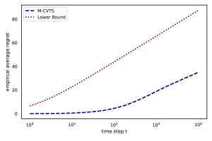
As an example of experiment with multinomial arms, we report in Table 1 the results of an experiment with 103superscript10310^{3} randomly generated problems with 555 arms drawn uniformly at random in 𝒫|𝒳|superscript𝒫𝒳\mathcal{P}^{|\mathcal{X}|}, where 𝒳=[0,0.1,0.2,,1]𝒳00.10.21\mathcal{X}=[0,0.1,0.2,\dots,1], for α{10%,50%,90%}𝛼percent10percent50percent90\alpha\in\{10\%,50\%,90\%\} and an horizon 104superscript10410^{4}. These experiments confirm the benefits of TS over UCB approaches, as M-CVTS significantly outperforms its competitors for all levels of the parameter α𝛼\alpha. We also tested the algorithms with fixed instances (see Tables 8-8), with the same results, and further illustrated the asymptotic optimality of M-CVTS in Figures 7 and  8 by representing the lower bound presented in Section 3 along with the regret of the algorithm in logarithmic scale.

We also tested B-CVTS on different problems, using truncated gaussian mixtures (TGM). The results are presented in Tables 9-12, and again show the merits of the TS approach. We also performed an experiment with a small level α=1%𝛼percent1\alpha=1\% (Table 13) and show that B-CVTS keeps the same level of performance in this case, while the other algorithm stay in the linear regime for the horizon we consider. Finally, we also experimented more arms (K=30𝐾30K=30) and randomly generated TGM problems and report the results in Table 2. The means and variance of each arm satisfy (μk,σk)𝒰([0.25,1]10×[0,0.1]10)similar-tosubscript𝜇𝑘subscript𝜎𝑘𝒰superscript0.25110superscript00.110(\mu_{k},\sigma_{k})\sim\mathcal{U}([0.25,1]^{1}0\times[0,0.1]^{1}0), and the probabilities of each mode are drawn uniformly, pk𝒟19similar-tosubscript𝑝𝑘subscript𝒟19p_{k}\sim\mathcal{D}_{19}.

Table 1: CVaR regret at time T=104𝑇superscript104T=10^{4}, averaged over 103superscript10310^{3} random instances with 555 multinomial arms supported on 𝒳=[0.1,0.2,,1]𝒳0.10.21\mathcal{X}=[0.1,0.2,\dots,1]

α𝛼\alpha U-UCB CVaR-UCB M-CVTS
10%percent1010\% 633.1 219.7 38.8
50%percent5050\% 368.8 187.9 48.9
90%percent9090\% 188.5 186.2 42.7
Table 2: Results for TGM arms with 10 modes, at T=10000𝑇10000T=10000 averaged over 400 random instances with K=30𝐾30K=30, α=5%𝛼percent5\alpha=5\% (results: mean (std)).
T U-UCB CVaR-UCB B-CVTS
10000 2149.9 (263) 2016.0 (265) 210.9 (6.4)
20000 4276.4 (538) 3781.3 (521) 237.1 (15.4)
40000 8493.4 (1085) 6894.1 (985) 263.5 (17.9)

These very good results with synthetic data and its theoretical guarantees motivate using the B-CVTS algorithm in the real-world application we introduce in the next section.

4.2 Bandit application in Agriculture

Motivation

Let us consider a farmer who must decide on a planting date (action) for a rainfed crop. Farmers have been reported to primarily seek advice that reduces uncertainty in highly uncertain decision making (McCown, 2002; Hochman and Carberry, 2011; Evans et al., 2017). Planting date is an example of such a decision as it will influence the probabilities of favorable meteorologic events during crop cultivation. These events are highly uncertain due to the length of crop growing cycles (e.g. 3 to 6 months for grain maize). For instance, because of the stochastic nature of the rainfalls and temperatures, a farmer will observe a range of different crop yields from year to year for the same planting date, all other technical choices being equal. Thus, assuming that the environment is stationary, each planting date corresponds to an underlying, unknown yield distribution, which can be modeled as an arm in a bandit problem. Depending on her profile, a farmer may be more or less risk averse, and the Conditional Value at Risk can be used to personalize her level of risk-aversion. For instance, a small-holder farmer looking for food security may seek to avoid very poor yields compromising auto-consumption (e.g α20%𝛼percent20\alpha\leq 20\%), while a market-oriented farmer may be more prone to risky choices in order to increase her profit but still not risk neutral (e.g α=80%𝛼percent80\alpha=80\%). Yield distributions are supposed to be bounded. Indeed, a finite yield potential can be defined under non-stressing conditions for a given crop and environment (Evans and Fischer, 1999; Tollenaar and Lee, 2002). Observed yields can be modeled as following Von Liebig’s law of minimum (Paris, 1992): limiting factors will determine how much of the yield potential can be expressed.
Refer to caption
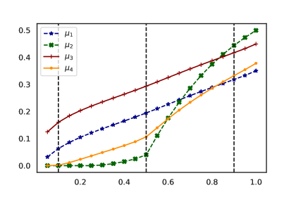
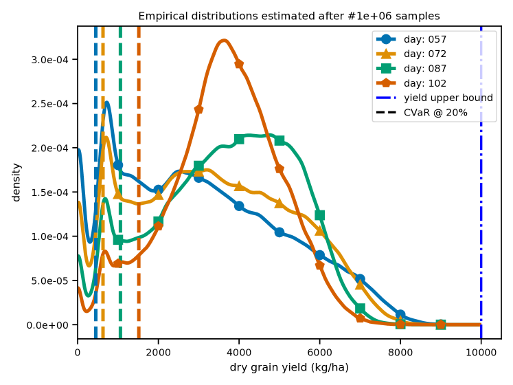
Figure 1: Empirical simulated yields and respective CVaRs at 20% estimated after 106superscript10610^{6} samples in DSSAT environment.
Setting

Planting date decision-making support requires extensive testing prior to any real-life application, due the potential impact of wrong action-making, particularly in subsistence farming. For this reason, we consider the problem of facing many times the decision of a planting date in the DSSAT333DSSAT is an Open-Source project maintained by the DSSAT Foundation, see https://dssat.net/. simulator, to make an in silico decision. DSSAT, standing for Decision Support System for Agrotechnology Transfer, is a world-wide crop simulator, supporting 42 different crops, with more than 30 years of development (Hoogenboom et al., 2019). We specifically address maize planting date decision, as maize is a crucial crop for global food security (Shiferaw et al., 2011). Each simulation is assumed to be realistic, and starts from the same field initial conditions as ground measured. The simulator takes as input historical weather data, field soil measures, crop specific genetic parameters and a given crop management plan. Modeling is based on simulations of atmospheric, soil and plants compartments and their interactions. In the considered experiments, after a decision is made on planting date in the simulator, daily stochastic meteorologic features are generated according to historical data (Richardson and Wright, 1984) and injected in the complex crop model. At the end of crop cycle, a maize grain yield is measured to evaluate decision-making. We parameterized the crop-model under challenging rainfed conditions on shallow sandy soils, i.e. with poor water retention and fertility. Such experiment intends to be representative of realistic conditions faced by small-holder farmers under heavy environmental constraints, such as in Sub-Saharan Africa. Thus, this setting can help picturing how CVaR bandits may perform in real-world conditions. For the sake of the experiments, we built a bandit-oriented Python wrapper to DSSAT that we made available444 https://github.com/rgautron/DssatBanditEnv to the bandit community for reproducibility.

Experiments

We test bandit performances on the 4 armed DSSAT environment described in Table 3. To illustrate the non-parametric nature of these distributions, we report in Figure 1 estimations of their density obtained with Monte-Carlo simulations, as well as of their CVaRs. The resulting distributions are typically multi-modal, with one of their mode very close to zero (years of bad harvest), and with upper tails that cannot be properly characterized. However the practitioner can realistically assume that the distributions are upper-bounded, due to the physical constraints of crop-farming. The yield upper-bound is set to 10 t/ha thanks to expert knowledge for the considered conditions.

Table 3: Empirical yield distribution metrics in kg/ha estimated after 106superscript10610^{6} samples in DSSAT environment
day (action). CVaRαsubscriptCVaR𝛼\text{CVaR}_{\alpha}
5%percent55\% 20%percent2020\% 80%percent8080\% 100%percent100100\% (mean)
057 0 448 2238 3016
072 46 627 2570 3273
087 287 1059 3074 3629
102 538 1515 3120 3586

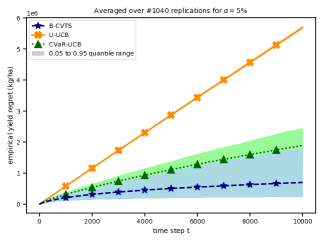
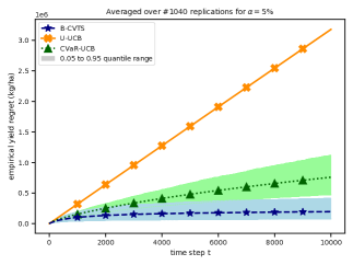
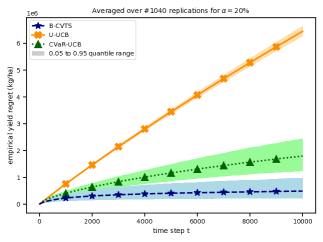
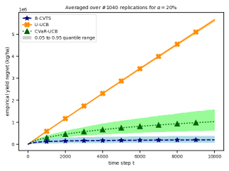
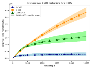
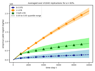
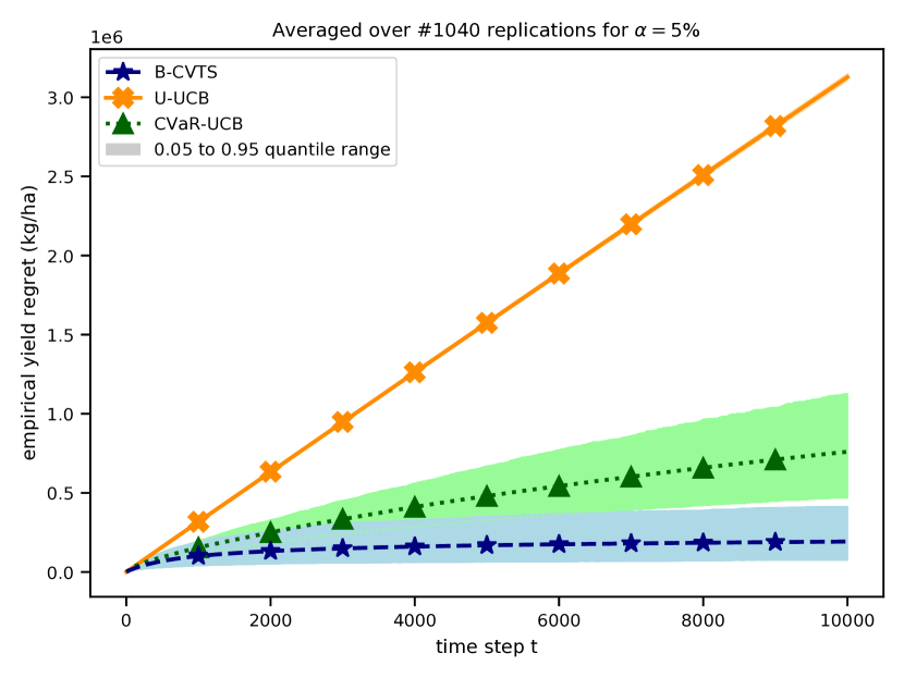
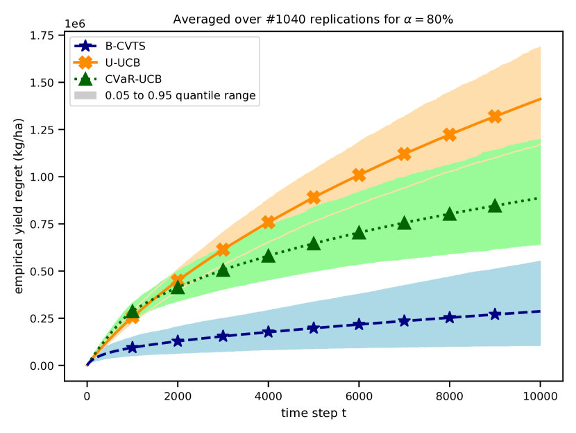
The presented DSSAT environment advocates for the use of algorithms specifically designed for CVaR bandits, as the optimal arm can change depending on the value of the parameter α𝛼\alpha. Our experiment consists in running 64 trajectories for three algorithms U-UCB, CVaR-UCB and B-CVTS defined in Section 2. Experiments are carried out with an horizon of 104superscript10410^{4} time steps, and we compare the results for each algorithm for α{5%,20%,80%}𝛼percent5percent20percent80\alpha\in\{5\%,20\%,80\%\} to see how the parameter impacts their performance. Indeed we want a strategy to perform well on all α𝛼\alpha choices, allowing to freely model any farmer’s risk aversion level. As shown in Figure 2 and Table 4, B-CVTS appears to be consistently better than its UCB counterparts in DSSAT environment for all tested α𝛼\alpha values, which is encouraging for real-life applications.

Table 4: Empirical yield regrets at horizon 104superscript10410^{4} in t/ha in DSSAT environment, for 1040 replications. Standard deviations in parenthesis.
α𝛼\alpha U-UCB CVaR-UCB B-CVTS
5%percent55\% 3128 (3) 760 (14) 192 (11)
20%percent2020\% 4867 (11) 1024 (17) 202 (10)
80%percent8080\% 1411 (13) 888 (13) 287 (12)

Further experiments are reported in Appendix G. In particular we increase the number of arms, and empirically study the effect of over-estimating the support upper-bound: our results show that a "prudent" bound has little effect of the performance of the algorithms in the settings we consider. This property is of particular interest for the practitioner, as a proper tuning of the support upper bound is the main limitation of the use of B-CVTS (and all bandit algorithms available for this problem). In most applications grounded on physical reality, the availability of such prudent upper-bound estimate is likely, and sufficient to ensure the practical performance of the B-CVTS algorithm.
Refer to caption
α=5%𝛼percent5\alpha=5\%
Refer to caption
α=80%𝛼percent80\alpha=80\%
Figure 2: Regret comparison in DSSAT environment, averaged over 1040 experiment replications.
Perspectives

This first set of experiments using a challenging realistic crop simulator is promising, and motivates to further investigate the use of B-CVTS algorithm for crop-management support and other problems that can be modeled as CVaR bandits. B-CVTS enjoys appealing theoretical guarantees, and thanks to its simplicity and competitive empirical performances may be a good candidate for practitioners. In order to address real-world crop-management challenges, many questions remain to be considered, e.g. how to optimally generate mini-batches of recommendations to an ensemble of farmers in a semi-sequential procedure (in order to account for the long feedback time), how to incorporate distribution priors on crop-management options that could be pre-learnt in silico and refining them adaptively in the real world (thus, minimizing random exploration in the real world), how to include contextual information such as soil characteristics and local weather forecasts, or how handle non-stationarity, incorporating climate change progressive impact on an optimal planting date. Furthermore, the simplicity of the Non-Parametric Thompson Sampling algorithms make them appealing for generalization to other risk-aware settings, e.g risk-constrained (maximizing the mean under a condition on the CVaR) or with other risk metrics (mean-variance, entropic risk, etc). All of these open questions make interesting challenges for future works.

Acknowledgements

This work has been supported by the French Ministry of Higher Education and Research, Hauts-de-France region, Inria within the team-project Scool and the MEL. The authors acknowledge the funding of the French National Research Agency under projects BADASS (ANR-16-CE40-0002) and BOLD (ANR-19-CE23-0026-04) and the I-Site ULNE regarding project R-PILOTE-19-004-APPRENF.

The PhD of Dorian Baudry is funded by a CNRS80 grant. The PhD of Romain Gautron is co-funded by the French Agricultural Research Centre for International Development (CIRAD) and the Consortium of International Agricultural Research Centers (CGIAR) Big Data Platfrom.

Experiments presented in this paper were carried out using the Grid’5000 testbed, supported by a scientific interest group hosted by Inria and including CNRS, RENATER and several Universities as well as other organizations (see https://www.grid5000.fr).

References

  • Acerbi and Tasche [2002] C. Acerbi and D. Tasche. On the coherence of expected shortfall. Journal of Banking & Finance, 26:1487–1503, 2002.
  • Agrawal and Goyal [2013] S. Agrawal and N. Goyal. Further Optimal Regret Bounds for Thompson Sampling. In Proceedings of the 16th Conference on Artificial Intelligence and Statistics, 2013.
  • Agrawal et al. [2020] S. Agrawal, W. M. Koolen, and S. Juneja. Optimal best-arm identification methods for tail-risk measures. arXiv preprint arXiv:2008.07606, 2020.
  • Artzner et al. [1999] P. Artzner, F. Delbaen, J.-M. Eber, and D. Heath. Coherent measures of risk. Mathematical Finance, 9:203–228, 1999.
  • Auer et al. [2002] P. Auer, N. Cesa-Bianchi, and P. Fischer. Finite-time analysis of the multiarmed bandit problem. Machine learning, 47, 2002.
  • Berge [1997] C. Berge. Topological Spaces: including a treatment of multi-valued functions, vector spaces, and convexity. 1997.
  • Brown [2007] D. Brown. Large deviations bounds for estimating conditional value-at-risk. Oper. Res. Lett., 35:722–730, 2007.
  • Burnetas and Katehakis [1996] A. Burnetas and M. Katehakis. Optimal adaptive policies for sequential allocation problems. Advances in Applied Mathematics, 17(2), 1996.
  • Cappé et al. [2013] O. Cappé, A. Garivier, O.-A. Maillard, R. Munos, and G. Stoltz. Kullback–leibler upper confidence bounds for optimal sequential allocation. The Annals of Statistics, 41, 2013.
  • Carpentier and Valko [2014] A. Carpentier and M. Valko. Extreme bandits. In Neural Information Processing Systems, Montréal, Canada, Dec. 2014.
  • Cassel et al. [2018] A. Cassel, S. Mannor, and A. Zeevi. A general approach to multi-armed bandits under risk criteria. In Proceedings of the 31st Annual Conference On Learning Theory, 2018.
  • Evans et al. [2017] K. J. Evans, A. Terhorst, and B. H. Kang. From data to decisions: helping crop producers build their actionable knowledge. Critical reviews in plant sciences, 36(2):71–88, 2017.
  • Evans and Fischer [1999] L. Evans and R. Fischer. Yield potential: its definition, measurement, and significance. Crop science, 39(6):1544–1551, 1999.
  • Galichet [2015] N. Galichet. Contributions to multi-armed bandits: Risk-awareness and sub-sampling for linear contextual bandits. PhD thesis, 2015.
  • Galichet et al. [2013] N. Galichet, M. Sebag, and O. Teytaud. Exploration vs exploitation vs safety: Risk-aware multi-armed bandits. In Asian Conference on Machine Learning, 2013.
  • Garivier et al. [2019] A. Garivier, P. Ménard, and G. Stoltz. Explore first, exploit next: The true shape of regret in bandit problems. Math. Oper. Res., 44:377–399, 2019.
  • Hochman and Carberry [2011] Z. Hochman and P. Carberry. Emerging consensus on desirable characteristics of tools to support farmers’ management of climate risk in australia. Agricultural Systems, 104(6):441–450, 2011.
  • Holland and Haress [2020] M. J. Holland and E. M. Haress. Learning with cvar-based feedback under potentially heavy tails, 2020.
  • Honda and Takemura [2010] J. Honda and A. Takemura. An Asymptotically Optimal Bandit Algorithm for Bounded Support Models. In Proceedings of the 23rd Annual Conference on Learning Theory, 2010.
  • Honda and Takemura [2015] J. Honda and A. Takemura. Non-asymptotic analysis of a new bandit algorithm for semi-bounded rewards. Journal of Machine Learning Research, 16:3721–3756, 2015.
  • Hoogenboom et al. [2019] G. Hoogenboom, C. Porter, K. Boote, V. Shelia, P. Wilkens, U. Singh, J. White, S. Asseng, J. Lizaso, L. Moreno, et al. The dssat crop modeling ecosystem. Advances in crop modelling for a sustainable agriculture, pages 173–216, 2019.
  • Kagrecha et al. [2019] A. Kagrecha, J. Nair, and K. P. Jagannathan. Distribution oblivious, risk-aware algorithms for multi-armed bandits with unbounded rewards. In Advances in Neural Information Processing Systems, 2019.
  • Kagrecha et al. [2020] A. Kagrecha, J. Nair, and K. P. Jagannathan. Constrained regret minimization for multi-criterion multi-armed bandits. 2020.
  • Kaufmann et al. [2012] E. Kaufmann, N. Korda, and R. Munos. Thompson sampling: An asymptotically optimal finite-time analysis. In Algorithmic Learning Theory - 23rd International Conference, ALT 2012, 2012.
  • Korda et al. [2013] N. Korda, E. Kaufmann, and R. Munos. Thompson Sampling for 1-dimensional Exponential family bandits. In Advances in Neural Information Processing Systems, 2013.
  • Lai and Robbins [1985] T. Lai and H. Robbins. Asymptotically efficient adaptive allocation rules. Advances in Applied Mathematics, 6, 1985.
  • Lattimore [2017] T. Lattimore. A scale free algorithm for stochastic bandits with bounded kurtosis. 2017.
  • Lattimore and Szepesvari [2019] T. Lattimore and C. Szepesvari. Bandit Algorithms. Cambridge University Press, 2019.
  • Maillard [2013] O. Maillard. Robust risk-averse stochastic multi-armed bandits. In Algorithmic Learning Theory - 24th International Conference, ALT, 2013.
  • Mandelbrot [1997] B. B. Mandelbrot. The variation of certain speculative prices. In Fractals and scaling in finance. Springer, 1997.
  • Massart [1990] P. Massart. The tight constant in the dvoretzky-kiefer-wolfowitz inequality. Annals of Probability, 18, 1990.
  • McCown [2002] R. L. McCown. Changing systems for supporting farmers’ decisions: problems, paradigms, and prospects. Agricultural systems, 74(1):179–220, 2002.
  • Paris [1992] Q. Paris. The return of von liebig’s “law of the minimum”. Agronomy Journal, 84(6):1040–1046, 1992.
  • Prashanth et al. [2020] L. A. Prashanth, P. Krishna, Jagannathan, and R. K. Kolla. Concentration bounds for cvar estimation: The cases of light-tailed and heavy-tailed distributions. In International Conference on Machine Learning, 2020.
  • Prashanth L et al. [2019] A. Prashanth L, K. Jagannathan, and R. K. Kolla. Concentration bounds for cvar estimation: The cases of light-tailed and heavy-tailed distributions. International Conference on Machine Learning, 2019.
  • Richardson and Wright [1984] C. W. Richardson and D. A. Wright. Wgen: A model for generating daily weather variables. ARS (USA), 1984.
  • Riou and Honda [2020] C. Riou and J. Honda. Bandit algorithms based on thompson sampling for bounded reward distributions. In Algorithmic Learning Theory - 31st International Conference, ALT 2020, 2020.
  • Rockafellar et al. [2000] R. T. Rockafellar, S. Uryasev, et al. Optimization of conditional value-at-risk. Journal of risk, 2:21–42, 2000.
  • Russo et al. [2018] D. Russo, B. V. Roy, A. Kazerouni, I. Osband, and Z. Wen. A tutorial on thompson sampling. Foundations and Trends in Machine Learning, 11:1–96, 2018.
  • Sani et al. [2012] A. Sani, A. Lazaric, and R. Munos. Risk-aversion in multi-armed bandits. In Advances in Neural Information Processing Systems, 2012.
  • Shiferaw et al. [2011] B. Shiferaw, B. M. Prasanna, J. Hellin, and M. Bänziger. Crops that feed the world 6. past successes and future challenges to the role played by maize in global food security. Food security, 3(3):307–327, 2011.
  • Szorenyi et al. [2015] B. Szorenyi, R. Busa-Fekete, P. Weng, and E. Hüllermeier. Qualitative multi-armed bandits: A quantile-based approach. In International Conference on Machine Learning, 2015.
  • Tamkin et al. [2020] A. Tamkin, R. Keramati, C. Dann, and E. Brunskill. Distributionally-aware exploration for cvar bandits. In NeurIPS 2019 Workshop on Safety and Robustness in Decision Making; RLDM 2019, 2020.
  • Thomas and Learned-Miller [2019] P. Thomas and E. Learned-Miller. Concentration inequalities for conditional value at risk. In International Conference on Machine Learning, 2019.
  • Thompson [1933] W. R. Thompson. On the likelihood that one unknown probability exceeds another in view of the evidence of two samples. Biometrika, 25, 1933.
  • Tollenaar and Lee [2002] M. Tollenaar and E. Lee. Yield potential, yield stability and stress tolerance in maize. Field crops research, 75(2-3):161–169, 2002.
  • Vakili and Zhao [2015] S. Vakili and Q. Zhao. Mean-variance and value at risk in multi-armed bandit problems. In 2015 53rd Annual Allerton Conference on Communication, Control, and Computing (Allerton), 2015.
  • Vakili and Zhao [2016] S. Vakili and Q. Zhao. Risk-averse multi-armed bandit problems under mean-variance measure. IEEE J. Sel. Top. Signal Process., 10:1093–1111, 2016.
  • Zhu and Tan [2020] Q. Zhu and V. Tan. Thompson sampling algorithms for mean-variance bandits. In Proceedings of the 37th International Conference on Machine Learning, 2020.
  • Zimin et al. [2014] A. Zimin, R. Ibsen-Jensen, and K. Chatterjee. Generalized risk-aversion in stochastic multi-armed bandits. CoRR, abs/1405.0833, 2014.

Appendix A Notations for the proofs

In this section, we introduce for convenience several notations that are used in the regret analysis.

A.1 General Notations

Model for multinomial arms

In section B we denote by (𝒳1,,𝒳K)subscript𝒳1subscript𝒳𝐾(\mathcal{X}_{1},\dots,\mathcal{X}_{K}) the supports of (ν1,,νK)subscript𝜈1subscript𝜈𝐾(\nu_{1},\dots,\nu_{K}), where 𝒳k=(x1k,,xMkk)subscript𝒳𝑘superscriptsubscript𝑥1𝑘superscriptsubscript𝑥subscript𝑀𝑘𝑘\mathcal{X}_{k}=(x_{1}^{k},\dots,x_{M_{k}}^{k}) for some integer Mksubscript𝑀𝑘M_{k}. We also denote 𝒫M={pM:i,pi0,j=1Mpj=1}superscript𝒫𝑀conditional-set𝑝superscript𝑀formulae-sequencefor-all𝑖subscript𝑝𝑖0superscriptsubscript𝑗1𝑀subscript𝑝𝑗1\mathcal{P}^{M}=\{p\in\mathbb{R}^{M}:\forall i,p_{i}\geq 0,\sum_{j=1}^{M}p_{j}=1\} the probability simplex in M+1superscript𝑀1\mathbb{R}^{M+1}. Any multinomial distribution ν𝜈\nu is characterized by its support and its probability vector pνsubscript𝑝𝜈p_{\nu}: ν=(𝒳,pν)𝜈𝒳subscript𝑝𝜈\nu=(\mathcal{X},p_{\nu}) with pν𝒫|𝒳|subscript𝑝𝜈superscript𝒫𝒳p_{\nu}\in\mathcal{P}^{|\mathcal{X}|}. Each arm νksubscript𝜈𝑘\nu_{k} is associated with a probability vector pk𝒫Msubscript𝑝𝑘superscript𝒫𝑀p_{k}\in\mathcal{P}^{M}.

Model for continuous bounded distributions

In section C we assume that each arm k𝑘k is supported in [0,Bk]0subscript𝐵𝑘[0,B_{k}] for some known value Bk>0subscript𝐵𝑘0B_{k}>0. We could assume supports of the form [ak,bk]subscript𝑎𝑘subscript𝑏𝑘[a_{k},b_{k}] where only an upper bound on each bksubscript𝑏𝑘b_{k} is known without loss of generality in the result, but we use this formulation for the sake of simplicity. We consider the set of continuous distributions in [0,Bk]0subscript𝐵𝑘[0,B_{k}], that we write 𝒞Bksuperscript𝒞subscript𝐵𝑘\mathcal{C}^{B_{k}}. We still denote 𝒫M={pM:i,pi0,j=1Mpj=1}superscript𝒫𝑀conditional-set𝑝superscript𝑀formulae-sequencefor-all𝑖subscript𝑝𝑖0superscriptsubscript𝑗1𝑀subscript𝑝𝑗1\mathcal{P}^{M}=\{p\in\mathbb{R}^{M}:\forall i,p_{i}\geq 0,\sum_{j=1}^{M}p_{j}=1\} the probability simplex in Msuperscript𝑀\mathbb{R}^{M}. The distribution of an arm k𝑘k is νksubscript𝜈𝑘\nu_{k}, and its CVaR at a level α𝛼\alpha is denoted ckαsuperscriptsubscript𝑐𝑘𝛼c_{k}^{\alpha}.

Notations for the CVaR

In the proofs in section of section B and section C we will encounter three different CVaR formulations for which we propose convenient notations,

  • CVaRα(F)subscriptCVaR𝛼𝐹\text{CVaR}_{\alpha}(F) for the CVaR of a distribution with a specified cumulative distribution function F𝐹F.

  • Cα(𝒳,w)subscript𝐶𝛼𝒳𝑤C_{\alpha}(\mathcal{X},w) for the CVaR of a discrete random variable of support 𝒳[0,B]𝒳0𝐵\mathcal{X}\subset[0,B] associated with a probability vector w𝒫|𝒳|𝑤superscript𝒫𝒳w\in\mathcal{P}^{|\mathcal{X}|}. According to our previous notation, Cα(𝒳,w)=CVaRα(Fw)subscript𝐶𝛼𝒳𝑤subscriptCVaR𝛼subscript𝐹𝑤C_{\alpha}(\mathcal{X},w)=\text{CVaR}_{\alpha}\left(F_{w}\right), where for all y𝑦y\in\mathbb{R},

    F(y)=1|𝒳|x𝒳wx𝟙(yx).𝐹𝑦1𝒳subscript𝑥𝒳subscript𝑤𝑥1𝑦𝑥F(y)=\frac{1}{|\mathcal{X}|}\sum_{x\in\mathcal{X}}w_{x}\mathds{1}(y\leq x)\;.
  • Cα(𝒳)subscript𝐶𝛼𝒳C_{\alpha}(\mathcal{X}) the CVaR of the uniform distribution on the discret support 𝒳𝒳\mathcal{X}, which shortens the notations for the CVaR of the empirical distributions: Cα(𝒳)=Cα(𝒳,1N)subscript𝐶𝛼𝒳subscript𝐶𝛼𝒳subscript1𝑁C_{\alpha}(\mathcal{X})=C_{\alpha}(\mathcal{X},1_{N}) where 1N=(1N,,1N)Ntermssubscript1𝑁subscript1𝑁1𝑁𝑁𝑡𝑒𝑟𝑚𝑠1_{N}=\underbrace{\left(\frac{1}{N},\dots,\frac{1}{N}\right)}_{Nterms}.

We also introduce ckα=CVaRα(Fk)superscriptsubscript𝑐𝑘𝛼subscriptCVaR𝛼subscript𝐹𝑘c_{k}^{\alpha}=\text{CVaR}_{\alpha}(F_{k}) the CVaR of each arm’s distribution, further assuming without loss of generality that

c1α=argmaxk{1,,K}ckα.superscriptsubscript𝑐1𝛼𝑘1𝐾argmaxsuperscriptsubscript𝑐𝑘𝛼c_{1}^{\alpha}=\underset{k\in\{1,\dots,K\}}{\text{argmax}}c_{k}^{\alpha}.
Algorithm

Both M-CVTS and B-CVTS can be formulated as an index policy, that is

At=argmaxk[K]ck,tα,subscript𝐴𝑡𝑘delimited-[]𝐾argmaxsuperscriptsubscript𝑐𝑘𝑡𝛼A_{t}=\underset{k\in[K]}{\text{argmax}}\ c_{k,t}^{\alpha},

where ck,tαsuperscriptsubscript𝑐𝑘𝑡𝛼c_{k,t}^{\alpha} is the index used in round t𝑡t. We recall that Nk(t)=s=1t𝟙(As=k)subscript𝑁𝑘𝑡superscriptsubscript𝑠1𝑡1subscript𝐴𝑠𝑘N_{k}(t)=\sum_{s=1}^{t}\mathds{1}(A_{s}=k) denotes the number of selections of arms k𝑘k. We define the σ𝜎\sigma-field t={Aτ,rAτ for τ={1,,t}}subscript𝑡subscript𝐴𝜏subscript𝑟subscript𝐴𝜏 for 𝜏1𝑡\mathcal{F}_{t}=\{A_{\tau},r_{A_{\tau}}\text{ for }\tau=\{1,\dots,t\}\}. In particular, knowing tsubscript𝑡\mathcal{F}_{t} allows to know Nk(t)subscript𝑁𝑘𝑡N_{k}(t) and the history of all arms available up to time t𝑡t (i.e. all observations drawn before and including t𝑡t).

Distances

We define for multinomial distributions with same support 𝒳𝒳\mathcal{X} the distance

d:𝒫|𝒳|×𝒫|𝒳|+:(p,q)pq=supm{1,,|𝒳|}|pmqm|.:𝑑superscript𝒫𝒳superscript𝒫𝒳superscript:𝑝𝑞subscriptnorm𝑝𝑞subscriptsupremum𝑚1𝒳subscript𝑝𝑚subscript𝑞𝑚d:\mathcal{P}^{|\mathcal{X}|}\times\mathcal{P}^{|\mathcal{X}|}\rightarrow\mathbb{R}^{+}:(p,q)\rightarrow||p-q||_{\infty}=\sup_{m\in\{1,\dots,|\mathcal{X}|\}}|p_{m}-q_{m}|\;.

We also introduce the notation DL(F,G)subscript𝐷𝐿𝐹𝐺D_{L}(F,G) for the Levy distance between two distributions with cdf F𝐹F, and G𝐺G. Namely, if two distributions are supported in [0,B]0𝐵[0,B] for some B>0𝐵0B>0

DL(F,G)=inf{ε>0:x[0,B],F(xε)εG(x)F(x+ε)+ε}.subscript𝐷𝐿𝐹𝐺infimumconditional-set𝜀0formulae-sequencefor-all𝑥0𝐵𝐹𝑥𝜀𝜀𝐺𝑥𝐹𝑥𝜀𝜀D_{L}(F,G)=\inf\left\{\operatorname{\varepsilon}>0:\forall x\in[0,B],F(x-\operatorname{\varepsilon})-\operatorname{\varepsilon}\leq G(x)\leq F(x+\operatorname{\varepsilon})+\operatorname{\varepsilon}\right\}\;.

Furthermore, we recall the result from [Riou and Honda, 2020] stating that for two distributions of cdf F𝐹F and G𝐺G,

DL(F,G)FGsubscript𝐷𝐿𝐹𝐺subscriptnorm𝐹𝐺D_{L}(F,G)\leq||F-G||_{\infty}

A.2 Specific notations for multinomial arms

We introduce for multinomial arms Nkm(t)superscriptsubscript𝑁𝑘𝑚𝑡N_{k}^{m}(t) as the number of times an element xmsubscript𝑥𝑚x_{m} has been observed during these pulls, so that Nk(t)=m=1MkNkm(t)subscript𝑁𝑘𝑡superscriptsubscript𝑚1subscript𝑀𝑘superscriptsubscript𝑁𝑘𝑚𝑡N_{k}(t)=\sum_{m=1}^{M_{k}}N_{k}^{m}(t). The Dirichlet posterior distribution given the observation after t𝑡t rounds is then Dir(βk,t)Dirsubscript𝛽𝑘𝑡\mathrm{Dir}(\beta_{k,t}) where βk,t=(1+Nk1(t1),1+Nk1(t1),,1+NkMk(t1))subscript𝛽𝑘𝑡1superscriptsubscript𝑁𝑘1𝑡11superscriptsubscript𝑁𝑘1𝑡11superscriptsubscript𝑁𝑘subscript𝑀𝑘𝑡1\beta_{k,t}=(1+N_{k}^{1}(t-1),1+N_{k}^{1}(t-1),\dots,1+N_{k}^{M_{k}}(t-1)). With this notation, the index is

ck,tα=Cα(𝒳k,wk,t)wherewk,tDir(βk,t).formulae-sequencesuperscriptsubscript𝑐𝑘𝑡𝛼subscript𝐶𝛼subscript𝒳𝑘subscript𝑤𝑘𝑡wheresimilar-tosubscript𝑤𝑘𝑡Dirsubscript𝛽𝑘𝑡c_{k,t}^{\alpha}=C_{\alpha}\left(\mathcal{X}_{k},w_{k,t}\right)\ \ \text{where}\ \ \ w_{k,t}\sim\mathrm{Dir}(\beta_{k,t}).

We denote by βk,tsubscript𝛽𝑘𝑡\beta_{k,t} the parameter of the Dirichlet distribution sampled at round t𝑡t for arm k𝑘k, and by pk,t𝒫Mksubscript𝑝𝑘𝑡superscript𝒫subscript𝑀𝑘p_{k,t}\in\mathcal{P}^{M_{k}} the mean of this Dirichlet distribution: pk,t=1Nk(t1)+Mkβk,tsubscript𝑝𝑘𝑡1subscript𝑁𝑘𝑡1subscript𝑀𝑘subscript𝛽𝑘𝑡p_{k,t}=\frac{1}{N_{k}(t-1)+M_{k}}\beta_{k,t}. Observe that this probability vector can also be viewed as a biased version of the empirical probability distribution of arm k𝑘k.

To ease the notation, we denote by 𝒳=(x1,,xM)𝒳subscript𝑥1subscript𝑥𝑀\mathcal{X}=(x_{1},\dots,x_{M}) the support of arm 111, while the support of any sub-optimal arm k𝑘k is denoted by 𝒳k=(x1k,,xMkk)subscript𝒳𝑘superscriptsubscript𝑥1𝑘superscriptsubscript𝑥subscript𝑀𝑘𝑘\mathcal{X}_{k}=(x_{1}^{k},\dots,x_{M_{k}}^{k}).

A.3 Notations for continuous arms

For continuous arms we simply write 𝒳nksuperscriptsubscript𝒳𝑛𝑘\mathcal{X}_{n}^{k} the history of observations available after n𝑛n pulls of armk𝑘k, X0k,X1k,X2k,,Xnksuperscriptsubscript𝑋0𝑘superscriptsubscript𝑋1𝑘superscriptsubscript𝑋2𝑘superscriptsubscript𝑋𝑛𝑘X_{0}^{k},X_{1}^{k},X_{2}^{k},\dots,X_{n}^{k} in the order they have been collected, including as first term X0k=Bksuperscriptsubscript𝑋0𝑘subscript𝐵𝑘X_{0}^{k}=B_{k}, the upper bound of the support of k𝑘k considered by the strategy. When considering (optimal) arm 111 we omit the exponent k𝑘k to simplify notations. The Dirichlet distributions that we consider in this case are always of the form Dir((1,,1))Dir11\text{Dir}((1,\dots,1)), where the size of the mean vector depends on the number of observation. We recall that this distribution is the uniform distribution on a simplex of fixed size N𝑁N, and its average is the vector (1N,,1N)1𝑁1𝑁\left(\frac{1}{N},\dots,\frac{1}{N}\right). We denote this distribution 𝒟Nsubscript𝒟𝑁\mathcal{D}_{N} to simplify the notations.

Appendix B Proof of Theorem 2 : analysis of M-CVTS with multinomial arms

Thanks to Equation (3) presented in Section 3, the proof of Theorem 2 can be obtained by proving Equation (4) and Equation (6) for multinomial arms distributions. This consists in upper bounding the pre-convergence (Pre-CV) and post-convergence (Post-CV) terms presented in section 3. In this section we use the Lsuperscript𝐿L^{\infty} distance presented in Section A.

B.1 Proof of Equation (4) : Upper Bound on the Post-Convergence term

We upper bound the term (Post-CV)=𝔼[t=1T𝟙(At=k,ck,tαc1αε1,d(pk,t,pk)ε2)](Post-CV)𝔼delimited-[]superscriptsubscript𝑡1𝑇1formulae-sequencesubscript𝐴𝑡𝑘formulae-sequencesuperscriptsubscript𝑐𝑘𝑡𝛼superscriptsubscript𝑐1𝛼subscript𝜀1𝑑subscript𝑝𝑘𝑡subscript𝑝𝑘subscript𝜀2\text{(Post-CV)}=\mathbb{E}\left[\sum_{t=1}^{T}\mathds{1}(A_{t}=k,c_{k,t}^{\alpha}\geq c_{1}^{\alpha}-\operatorname{\varepsilon}_{1},d(p_{k,t},p_{k})\leq\operatorname{\varepsilon}_{2})\right], where pk,t=βk,tNk(t1)subscript𝑝𝑘𝑡subscript𝛽𝑘𝑡subscript𝑁𝑘𝑡1p_{k,t}=\frac{\beta_{k,t}}{N_{k}(t-1)} is the probability vector associated with the empirical distribution of an arm k𝑘k, i.e the frequency of each item of the support 𝒳ksubscript𝒳𝑘\mathcal{X}_{k} in the history of arm k𝑘k. We recall that this former quantity is biased because of the initialization step which set βk,0=(1,,1)subscript𝛽𝑘011\beta_{k,0}=(1,\dots,1) and Nki(0)=1superscriptsubscript𝑁𝑘𝑖01N_{k}^{i}(0)=1 (introducing the fictitious time t=0𝑡0t=0 just before the algorithms starts). For any constant n0(T)subscript𝑛0𝑇n_{0}(T) we have

(Post-CV)(Post-CV)absent\displaystyle\text{(Post-CV)}\leq 𝔼[t=1T𝟙(At=k,ck,tαc1αε1,d(pk,t,pk)ε2)]𝔼delimited-[]superscriptsubscript𝑡1𝑇1formulae-sequencesubscript𝐴𝑡𝑘formulae-sequencesuperscriptsubscript𝑐𝑘𝑡𝛼superscriptsubscript𝑐1𝛼subscript𝜀1𝑑subscript𝑝𝑘𝑡subscript𝑝𝑘subscript𝜀2\displaystyle\mathbb{E}\left[\sum_{t=1}^{T}\mathds{1}(A_{t}=k,c_{k,t}^{\alpha}\geq c_{1}^{\alpha}-\operatorname{\varepsilon}_{1},d(p_{k,t},p_{k})\leq\operatorname{\varepsilon}_{2})\right]
\displaystyle\leq t=1T𝔼[𝟙(At=k,Nk(t1)n0(T),ck,tαc1αε1,d(pk,t,pk)ε2)]superscriptsubscript𝑡1𝑇𝔼delimited-[]1formulae-sequencesubscript𝐴𝑡𝑘formulae-sequencesubscript𝑁𝑘𝑡1subscript𝑛0𝑇formulae-sequencesuperscriptsubscript𝑐𝑘𝑡𝛼superscriptsubscript𝑐1𝛼subscript𝜀1𝑑subscript𝑝𝑘𝑡subscript𝑝𝑘subscript𝜀2\displaystyle\sum_{t=1}^{T}\mathbb{E}\left[\mathds{1}(A_{t}=k,N_{k}(t-1)\leq n_{0}(T),c_{k,t}^{\alpha}\geq c_{1}^{\alpha}-\operatorname{\varepsilon}_{1},d(p_{k,t},p_{k})\leq\operatorname{\varepsilon}_{2})\right]
+t=1T𝔼[𝟙(At=k,Nk(t1)n0(T),ck,tαc1αε1,d(pk,t,pk)ε2)].superscriptsubscript𝑡1𝑇𝔼delimited-[]1formulae-sequencesubscript𝐴𝑡𝑘formulae-sequencesubscript𝑁𝑘𝑡1subscript𝑛0𝑇formulae-sequencesuperscriptsubscript𝑐𝑘𝑡𝛼superscriptsubscript𝑐1𝛼subscript𝜀1𝑑subscript𝑝𝑘𝑡subscript𝑝𝑘subscript𝜀2\displaystyle+\sum_{t=1}^{T}\mathbb{E}\left[\mathds{1}(A_{t}=k,N_{k}(t-1)\geq n_{0}(T),c_{k,t}^{\alpha}\geq c_{1}^{\alpha}-\operatorname{\varepsilon}_{1},d(p_{k,t},p_{k})\leq\operatorname{\varepsilon}_{2})\right]\;.

The first term is upper bounded by n0(T)subscript𝑛0𝑇n_{0}(T) as the event (At=k,Nk(t1)n0(T))formulae-sequencesubscript𝐴𝑡𝑘subscript𝑁𝑘𝑡1subscript𝑛0𝑇(A_{t}=k,N_{k}(t-1)\leq n_{0}(T)) can occur at most n0(T)subscript𝑛0𝑇n_{0}(T) times. So we have

(Post-CV)(Post-CV)absent\displaystyle\text{(Post-CV)}\leq n0(T)+t=1T𝔼[𝟙(At=k,Nk(t1)n0(T),ck,tαc1αε1,d(pk,t,pk)ε2)]subscript𝑛0𝑇superscriptsubscript𝑡1𝑇𝔼delimited-[]1formulae-sequencesubscript𝐴𝑡𝑘formulae-sequencesubscript𝑁𝑘𝑡1subscript𝑛0𝑇formulae-sequencesuperscriptsubscript𝑐𝑘𝑡𝛼superscriptsubscript𝑐1𝛼subscript𝜀1𝑑subscript𝑝𝑘𝑡subscript𝑝𝑘subscript𝜀2\displaystyle n_{0}(T)+\sum_{t=1}^{T}\mathbb{E}\left[\mathds{1}(A_{t}=k,N_{k}(t-1)\geq n_{0}(T),c_{k,t}^{\alpha}\geq c_{1}^{\alpha}-\operatorname{\varepsilon}_{1},d(p_{k,t},p_{k})\leq\operatorname{\varepsilon}_{2})\right]
\displaystyle\leq n0(T)+t=1T𝔼[𝟙(Nk(t1)n0(T),ck,tαc1αε1,d(pk,t,pk)ε2)]subscript𝑛0𝑇superscriptsubscript𝑡1𝑇𝔼delimited-[]1formulae-sequencesubscript𝑁𝑘𝑡1subscript𝑛0𝑇formulae-sequencesuperscriptsubscript𝑐𝑘𝑡𝛼superscriptsubscript𝑐1𝛼subscript𝜀1𝑑subscript𝑝𝑘𝑡subscript𝑝𝑘subscript𝜀2\displaystyle n_{0}(T)+\sum_{t=1}^{T}\mathbb{E}\left[\mathds{1}(N_{k}(t-1)\geq n_{0}(T),c_{k,t}^{\alpha}\geq c_{1}^{\alpha}-\operatorname{\varepsilon}_{1},d(p_{k,t},p_{k})\leq\operatorname{\varepsilon}_{2})\right]
\displaystyle\leq n0(T)+t=1T𝔼[𝟙(Nk(t1)n0(T),d(pk,t,pk)ε2)×𝔼[𝟙(ck,tαc1αε1)|t1]]subscript𝑛0𝑇superscriptsubscript𝑡1𝑇𝔼delimited-[]1formulae-sequencesubscript𝑁𝑘𝑡1subscript𝑛0𝑇𝑑subscript𝑝𝑘𝑡subscript𝑝𝑘subscript𝜀2𝔼delimited-[]conditional1superscriptsubscript𝑐𝑘𝑡𝛼superscriptsubscript𝑐1𝛼subscript𝜀1subscript𝑡1\displaystyle n_{0}(T)+\sum_{t=1}^{T}\mathbb{E}\left[\mathds{1}\left(N_{k}(t-1)\geq n_{0}(T),d(p_{k,t},p_{k})\leq\operatorname{\varepsilon}_{2}\right)\times\mathbb{E}\left[\mathds{1}\left(c_{k,t}^{\alpha}\geq c_{1}^{\alpha}-\operatorname{\varepsilon}_{1}\right)|\mathcal{F}_{t-1}\right]\right]
=\displaystyle= n0(T)+t=1T𝔼[𝟙(Nk(t1)n0(T),d(pk,t,pk)ε2)×wDir(βk,t)(Cα(𝒳k,w)c1αε1)],subscript𝑛0𝑇superscriptsubscript𝑡1𝑇𝔼delimited-[]1formulae-sequencesubscript𝑁𝑘𝑡1subscript𝑛0𝑇𝑑subscript𝑝𝑘𝑡subscript𝑝𝑘subscript𝜀2subscriptsimilar-to𝑤Dirsubscript𝛽𝑘𝑡subscript𝐶𝛼subscript𝒳𝑘𝑤superscriptsubscript𝑐1𝛼subscript𝜀1\displaystyle n_{0}(T)+\sum_{t=1}^{T}\mathbb{E}\left[\mathds{1}\left(N_{k}(t-1)\geq n_{0}(T),d(p_{k,t},p_{k})\leq\operatorname{\varepsilon}_{2}\right)\times\mathbb{P}_{w\sim\mathrm{Dir}(\beta_{k,t})}\left(C_{\alpha}(\mathcal{X}_{k},w)\geq c_{1}^{\alpha}-\operatorname{\varepsilon}_{1}\right)\right]\;,

where we upper bounded 𝟙(At=k)1subscript𝐴𝑡𝑘\mathds{1}(A_{t}=k) by 111, so that 𝟙(ck,tαc1αε1)1superscriptsubscript𝑐𝑘𝑡𝛼superscriptsubscript𝑐1𝛼subscript𝜀1\mathds{1}\left(c_{k,t}^{\alpha}\geq c_{1}^{\alpha}-\operatorname{\varepsilon}_{1}\right) is the only term that is not t1subscript𝑡1\mathcal{F}_{t-1}-measurable, and then used the law of total expectation. Now we can use Lemma 1 to control the probability term inside the expectation by

wDir(βk(t))(Cα(𝒳k,w)c1αε1)C1Mk(Nk(t1)+Mk)Mk2exp((Nk(t1)+Mk)𝒦infα,𝒳k(pk,t,c1αε1)).subscriptsimilar-to𝑤Dirsubscript𝛽𝑘𝑡subscript𝐶𝛼subscript𝒳𝑘𝑤superscriptsubscript𝑐1𝛼subscript𝜀1subscript𝐶1subscript𝑀𝑘superscriptsubscript𝑁𝑘𝑡1subscript𝑀𝑘subscript𝑀𝑘2subscript𝑁𝑘𝑡1subscript𝑀𝑘superscriptsubscript𝒦infimum𝛼subscript𝒳𝑘subscript𝑝𝑘𝑡superscriptsubscript𝑐1𝛼subscript𝜀1\mathbb{P}_{w\sim\mathrm{Dir}(\beta_{k}(t))}\left(C_{\alpha}(\mathcal{X}_{k},w)\geq c_{1}^{\alpha}-\operatorname{\varepsilon}_{1}\right)\leq C_{1}M_{k}(N_{k}(t-1)+M_{k})^{\frac{M_{k}}{2}}\exp\left(-(N_{k}(t-1)+M_{k})\mathcal{K}_{\inf}^{\alpha,\mathcal{X}_{k}}(p_{k,t},c_{1}^{\alpha}-\operatorname{\varepsilon}_{1})\right).

At this stage, our objective is to remove the randomness in this upper bound in order to bound uniformly the terms inside the expectation. To do this, we will use the fact that d(pk,t,pk)ε2𝑑subscript𝑝𝑘𝑡subscript𝑝𝑘subscript𝜀2d(p_{k,t},p_{k})\leq\operatorname{\varepsilon}_{2} and Nk(t1)n0(T)subscript𝑁𝑘𝑡1subscript𝑛0𝑇N_{k}(t-1)\geq n_{0}(T) together with the continuity of the function 𝒦infα,𝒳ksuperscriptsubscript𝒦infimum𝛼subscript𝒳𝑘\mathcal{K}_{\inf}^{\alpha,\mathcal{X}_{k}} in its second argument, established in Lemma 6 defined in Appendix D.3.

Let ε3(0,𝒦infα,𝒳k(pk,t,c1α))subscript𝜀30superscriptsubscript𝒦infimum𝛼subscript𝒳𝑘subscript𝑝𝑘𝑡superscriptsubscript𝑐1𝛼\varepsilon_{3}\in(0,\mathcal{K}_{\inf}^{\alpha,\mathcal{X}_{k}}(p_{k,t},c_{1}^{\alpha})). There exists by continuity small enough values of ε1subscript𝜀1\varepsilon_{1} and ε2subscript𝜀2\varepsilon_{2} such that, if d(pk,t,pk)ε2𝑑subscript𝑝𝑘𝑡subscript𝑝𝑘subscript𝜀2d(p_{k,t},p_{k})\leq\varepsilon_{2},

𝒦infα,𝒳k(pk,t,c1αε1)superscriptsubscript𝒦infimum𝛼subscript𝒳𝑘subscript𝑝𝑘𝑡superscriptsubscript𝑐1𝛼subscript𝜀1\displaystyle\mathcal{K}_{\inf}^{\alpha,\mathcal{X}_{k}}(p_{k,t},c_{1}^{\alpha}-\operatorname{\varepsilon}_{1}) 𝒦infα,𝒳k(pk,c1αε1)ε34𝒦infα,𝒳k(pk,c1α)ε32,absentsuperscriptsubscript𝒦infimum𝛼subscript𝒳𝑘subscript𝑝𝑘superscriptsubscript𝑐1𝛼subscript𝜀1subscript𝜀34superscriptsubscript𝒦infimum𝛼subscript𝒳𝑘subscript𝑝𝑘superscriptsubscript𝑐1𝛼subscript𝜀32\displaystyle\geq\mathcal{K}_{\inf}^{\alpha,\mathcal{X}_{k}}(p_{k},c_{1}^{\alpha}-\operatorname{\varepsilon}_{1})-\frac{\operatorname{\varepsilon}_{3}}{4}\geq\mathcal{K}_{\inf}^{\alpha,\mathcal{X}_{k}}(p_{k},c_{1}^{\alpha})-\frac{\operatorname{\varepsilon}_{3}}{2},

hence

D:=(Nk(t1)+Mk)Mk2exp((Nk(t1)+Mk)𝒦infα,𝒳k(pk,t,c1αε1))assign𝐷superscriptsubscript𝑁𝑘𝑡1subscript𝑀𝑘subscript𝑀𝑘2subscript𝑁𝑘𝑡1subscript𝑀𝑘superscriptsubscript𝒦infimum𝛼subscript𝒳𝑘subscript𝑝𝑘𝑡superscriptsubscript𝑐1𝛼subscript𝜀1\displaystyle D:=(N_{k}(t-1)+M_{k})^{\frac{M_{k}}{2}}\exp\left(-(N_{k}(t-1)+M_{k})\mathcal{K}_{\inf}^{\alpha,\mathcal{X}_{k}}(p_{k,t},c_{1}^{\alpha}-\operatorname{\varepsilon}_{1})\right)
(Nk(t1)+Mk)Mk2exp((Nk(t1)+Mk)(𝒦infα,𝒳k(pk,c1α)ε3/2)).absentsuperscriptsubscript𝑁𝑘𝑡1subscript𝑀𝑘subscript𝑀𝑘2subscript𝑁𝑘𝑡1subscript𝑀𝑘superscriptsubscript𝒦infimum𝛼subscript𝒳𝑘subscript𝑝𝑘superscriptsubscript𝑐1𝛼subscript𝜀32\displaystyle\leq(N_{k}(t-1)+M_{k})^{\frac{M_{k}}{2}}\exp\left(-(N_{k}(t-1)+M_{k})(\mathcal{K}_{\inf}^{\alpha,\mathcal{X}_{k}}(p_{k},c_{1}^{\alpha})-\operatorname{\varepsilon}_{3}/2)\right).

Using the fact that for any b>0𝑏0b>0 and b>ε>0𝑏𝜀0b>\operatorname{\varepsilon}>0 there exists a constant Csuperscript𝐶C^{\prime} such that t>0for-all𝑡0\forall t>0: texp(bt)Cexp(t(bε))𝑡𝑏𝑡superscript𝐶𝑡𝑏𝜀t\exp(-bt)\leq C^{\prime}\exp(-t(b-\operatorname{\varepsilon})), we further get

D𝐷\displaystyle D Cexp((Nk(t1)+Mk)(𝒦infα,𝒳k(pk,c1α)ε3))absentsuperscript𝐶subscript𝑁𝑘𝑡1subscript𝑀𝑘superscriptsubscript𝒦infimum𝛼subscript𝒳𝑘subscript𝑝𝑘superscriptsubscript𝑐1𝛼subscript𝜀3\displaystyle\leq C^{\prime}\exp\left(-(N_{k}(t-1)+M_{k})(\mathcal{K}_{\inf}^{\alpha,\mathcal{X}_{k}}(p_{k},c_{1}^{\alpha})-\operatorname{\varepsilon}_{3})\right)
Cexp((n0(T)+Mk)(𝒦infα,𝒳k(pk,c1α)ε3)),absentsuperscript𝐶subscript𝑛0𝑇subscript𝑀𝑘superscriptsubscript𝒦infimum𝛼subscript𝒳𝑘subscript𝑝𝑘superscriptsubscript𝑐1𝛼subscript𝜀3\displaystyle\leq C^{\prime}\exp\left(-(n_{0}(T)+M_{k})(\mathcal{K}_{\inf}^{\alpha,\mathcal{X}_{k}}(p_{k},c_{1}^{\alpha})-\operatorname{\varepsilon}_{3})\right),

provided that Nk(t1)n0(T)subscript𝑁𝑘𝑡1subscript𝑛0𝑇N_{k}(t-1)\geq n_{0}(T).

Putting things together, we proved that for every ε3(0,𝒦infα,𝒳k(pk,t,c1α))subscript𝜀30superscriptsubscript𝒦infimum𝛼subscript𝒳𝑘subscript𝑝𝑘𝑡superscriptsubscript𝑐1𝛼\varepsilon_{3}\in(0,\mathcal{K}_{\inf}^{\alpha,\mathcal{X}_{k}}(p_{k,t},c_{1}^{\alpha})), if ε1subscript𝜀1\varepsilon_{1} and ε2subscript𝜀2\varepsilon_{2} are small enough, then there exists a constant C1>0superscriptsubscript𝐶10C_{1}^{\prime}>0 such that

(Post-CV)(Post-CV)absent\displaystyle\text{(Post-CV)}\leq n0(T)+t=1TC1exp((n0(T)+Mk)(𝒦infα,𝒳k(pk,c1α)ε3))subscript𝑛0𝑇superscriptsubscript𝑡1𝑇superscriptsubscript𝐶1subscript𝑛0𝑇subscript𝑀𝑘superscriptsubscript𝒦infimum𝛼subscript𝒳𝑘subscript𝑝𝑘superscriptsubscript𝑐1𝛼subscript𝜀3\displaystyle n_{0}(T)+\sum_{t=1}^{T}C_{1}^{\prime}\exp\left(-(n_{0}(T)+M_{k})(\mathcal{K}_{\inf}^{\alpha,\mathcal{X}_{k}}\left(p_{k},c_{1}^{\alpha}\right)-\operatorname{\varepsilon}_{3})\right)
\displaystyle\leq n0(T)+TC1exp((n0(T)+Mk)(𝒦infα,𝒳k(pk,c1α)ε3)).subscript𝑛0𝑇𝑇superscriptsubscript𝐶1subscript𝑛0𝑇subscript𝑀𝑘superscriptsubscript𝒦infimum𝛼subscript𝒳𝑘subscript𝑝𝑘superscriptsubscript𝑐1𝛼subscript𝜀3\displaystyle n_{0}(T)+TC_{1}^{\prime}\exp\left(-(n_{0}(T)+M_{k})(\mathcal{K}_{\inf}^{\alpha,\mathcal{X}_{k}}\left(p_{k},c_{1}^{\alpha}\right)-\operatorname{\varepsilon}_{3})\right).

Choosing n0(T)=logT𝒦infα,𝒳k(νk,c1αε1)ε3(Mk+1)subscript𝑛0𝑇𝑇superscriptsubscript𝒦infimum𝛼subscript𝒳𝑘subscript𝜈𝑘superscriptsubscript𝑐1𝛼subscript𝜀1subscript𝜀3subscript𝑀𝑘1n_{0}(T)=\frac{\log T}{\mathcal{K}_{\inf}^{\alpha,\mathcal{X}_{k}}\left(\nu_{k},c_{1}^{\alpha}-\operatorname{\varepsilon}_{1}\right)-\operatorname{\varepsilon}_{3}}-(M_{k}+1) yields the upper bound

(Post-CV)logT𝒦infα,𝒳k(pk,c1α)ε3+O(1).Post-CV𝑇superscriptsubscript𝒦infimum𝛼subscript𝒳𝑘subscript𝑝𝑘superscriptsubscript𝑐1𝛼subscript𝜀3𝑂1(\text{Post-CV})\leq\frac{\log T}{\mathcal{K}_{\inf}^{\alpha,\mathcal{X}_{k}}\left(p_{k},c_{1}^{\alpha}\right)-\operatorname{\varepsilon}_{3}}+O(1).

Finally, we have shown that for any ε0>0subscript𝜀00\operatorname{\varepsilon}_{0}>0, if ε1subscript𝜀1\varepsilon_{1} and ε2subscript𝜀2\varepsilon_{2} are small enough, then

(Post-CV)(1+ε0)logT𝒦infα,𝒳k(pk,c1α)+O(1),Post-CV1subscript𝜀0𝑇superscriptsubscript𝒦infimum𝛼subscript𝒳𝑘subscript𝑝𝑘superscriptsubscript𝑐1𝛼𝑂1(\text{Post-CV})\leq\frac{(1+\operatorname{\varepsilon}_{0})\log T}{\mathcal{K}_{\inf}^{\alpha,\mathcal{X}_{k}}\left(p_{k},c_{1}^{\alpha}\right)}+O(1),

which proves Equation (4).

B.2 Proof of Equation (6): Upper Bound on the Pre-Convergence term for multinomial distributions

In this section, we upper bound the term (Pre-CV)=𝔼(t=1T𝟙(At=k,{ck,tα<c1αε1d(pk,t,pk)>ε2}))(Pre-CV)𝔼superscriptsubscript𝑡1𝑇1subscript𝐴𝑡𝑘superscriptsubscript𝑐𝑘𝑡𝛼expectationsuperscriptsubscript𝑐1𝛼subscript𝜀1𝑑subscript𝑝𝑘𝑡subscript𝑝𝑘subscript𝜀2\text{(Pre-CV)}=\mathbb{E}\left(\sum_{t=1}^{T}\mathds{1}(A_{t}=k,\{c_{k,t}^{\alpha}<c_{1}^{\alpha}-\operatorname{\varepsilon}_{1}\cup d(p_{k,t},p_{k})>\operatorname{\varepsilon}_{2}\})\right).

We first decompose this term into

(Pre-CV)𝔼(t=1T𝟙(At=k,ck,tα<c1αε1))+𝔼(t=1T𝟙(At=k,d(pk,t,pk)>ε2)).(Pre-CV)𝔼superscriptsubscript𝑡1𝑇1formulae-sequencesubscript𝐴𝑡𝑘superscriptsubscript𝑐𝑘𝑡𝛼superscriptsubscript𝑐1𝛼subscript𝜀1𝔼superscriptsubscript𝑡1𝑇1formulae-sequencesubscript𝐴𝑡𝑘𝑑subscript𝑝𝑘𝑡subscript𝑝𝑘subscript𝜀2\text{(Pre-CV)}\leq\mathbb{E}\left(\sum_{t=1}^{T}\mathds{1}(A_{t}=k,c_{k,t}^{\alpha}<c_{1}^{\alpha}-\operatorname{\varepsilon}_{1})\right)+\mathbb{E}\left(\sum_{t=1}^{T}\mathds{1}(A_{t}=k,d(p_{k,t},p_{k})>\operatorname{\varepsilon}_{2})\right)\,.

Let us remark that the second term does not feature any CVaR, hence we can directly use the upper bound derived by [Riou and Honda, 2020] to get that, for any ε2>0subscript𝜀20\varepsilon_{2}>0,

𝔼(t=1T𝟙(At=k,d(pk,t,pk)>ε2))KM(2Mε2+2ε22).𝔼superscriptsubscript𝑡1𝑇1formulae-sequencesubscript𝐴𝑡𝑘𝑑subscript𝑝𝑘𝑡subscript𝑝𝑘subscript𝜀2𝐾𝑀2𝑀subscript𝜀22superscriptsubscript𝜀22\mathbb{E}\left(\sum_{t=1}^{T}\mathds{1}(A_{t}=k,d(p_{k,t},p_{k})>\operatorname{\varepsilon}_{2})\right)\leq KM\left(\frac{2M}{\operatorname{\varepsilon}_{2}}+\frac{2}{\operatorname{\varepsilon}_{2}^{2}}\right).

Hence, it remains to upper bound the term

A:=𝔼(t=1T𝟙(At=k,ck,tα<c1αε1))assign𝐴𝔼superscriptsubscript𝑡1𝑇1formulae-sequencesubscript𝐴𝑡𝑘superscriptsubscript𝑐𝑘𝑡𝛼superscriptsubscript𝑐1𝛼subscript𝜀1A:=\mathbb{E}\left(\sum_{t=1}^{T}\mathds{1}(A_{t}=k,c_{k,t}^{\alpha}<c_{1}^{\alpha}-\operatorname{\varepsilon}_{1})\right)

We write

A𝐴absent\displaystyle A\leq 𝔼[t=1T𝟙(cAt,tα<c1αε1)]𝔼delimited-[]superscriptsubscript𝑡1𝑇1superscriptsubscript𝑐subscript𝐴𝑡𝑡𝛼superscriptsubscript𝑐1𝛼subscript𝜀1\displaystyle\mathbb{E}\left[\sum_{t=1}^{T}\mathds{1}(c_{A_{t},t}^{\alpha}<c_{1}^{\alpha}-\operatorname{\varepsilon}_{1})\right]
\displaystyle\leq t=1Tn=1T𝔼[𝟙(cAt,tα<c1αε1,N1(t)=n)]superscriptsubscript𝑡1𝑇superscriptsubscript𝑛1𝑇𝔼delimited-[]1formulae-sequencesuperscriptsubscript𝑐subscript𝐴𝑡𝑡𝛼superscriptsubscript𝑐1𝛼subscript𝜀1subscript𝑁1𝑡𝑛\displaystyle\sum_{t=1}^{T}\sum_{n=1}^{T}\mathbb{E}\left[\mathds{1}(c_{A_{t},t}^{\alpha}<c_{1}^{\alpha}-\operatorname{\varepsilon}_{1},N_{1}(t)=n)\right]
\displaystyle\leq m=1Tn=1T𝔼[𝟙(t=1T𝟙(cAt,tα<c1αε1,N1(t)=n)m)],superscriptsubscript𝑚1𝑇superscriptsubscript𝑛1𝑇𝔼delimited-[]1superscriptsubscript𝑡1𝑇1formulae-sequencesuperscriptsubscript𝑐subscript𝐴𝑡𝑡𝛼superscriptsubscript𝑐1𝛼subscript𝜀1subscript𝑁1𝑡𝑛𝑚\displaystyle\sum_{m=1}^{T}\sum_{n=1}^{T}\mathbb{E}\left[\mathds{1}\left(\sum_{t=1}^{T}\mathds{1}(c_{A_{t},t}^{\alpha}<c_{1}^{\alpha}-\operatorname{\varepsilon}_{1},N_{1}(t)=n)\geq m\right)\right]\;,

where we used as in [Riou and Honda, 2020] that for any series of events (Et)subscript𝐸𝑡(E_{t}) it holds that

t=1T𝟙(Et)m=1T𝟙(t=1T𝟙(Et)m).superscriptsubscript𝑡1𝑇1subscript𝐸𝑡superscriptsubscript𝑚1𝑇1superscriptsubscript𝑡1𝑇1subscript𝐸𝑡𝑚\sum_{t=1}^{T}\mathds{1}(E_{t})\leq\sum_{m=1}^{T}\mathds{1}\left(\sum_{t=1}^{T}\mathds{1}(E_{t})\geq m\right).

We then introduce a random sequence (τin)isubscriptsuperscriptsubscript𝜏𝑖𝑛𝑖(\tau_{i}^{n})_{i\in\mathbb{N}} where τin{+}superscriptsubscript𝜏𝑖𝑛\tau_{i}^{n}\in\mathbb{R}\cup\{+\infty\} is the i𝑖i-th time at which the event {maxj>1cj,tαc1αε1,N1(t)=n}formulae-sequencesubscript𝑗1superscriptsubscript𝑐𝑗𝑡𝛼superscriptsubscript𝑐1𝛼subscript𝜀1subscript𝑁1𝑡𝑛\{\max_{j>1}c_{j,t}^{\alpha}\!\leq\!c_{1}^{\alpha}\!-\!\operatorname{\varepsilon}_{1},N_{1}(t)\!=\!n\} holds. In order to ensure that this event occurs at least m𝑚m times, then we need 1) that τin+superscriptsubscript𝜏𝑖𝑛\tau_{i}^{n}\leq+\infty for all im𝑖𝑚i\leq m, and 2) c1,τinαc1αε1superscriptsubscript𝑐1superscriptsubscript𝜏𝑖𝑛𝛼superscriptsubscript𝑐1𝛼subscript𝜀1c_{1,\tau_{i}^{n}}^{\alpha}\leq c_{1}^{\alpha}-\operatorname{\varepsilon}_{1} for all im𝑖𝑚i\leq m, otherwise arm 111 would be drawn. Hence, we have the following inclusion of events

{t=1T𝟙(cAt,tα<c1αε1,N1(t)=n)m}{τin<+,c1,τinαc1αε1i{1,,m}}.superscriptsubscript𝑡1𝑇1formulae-sequencesuperscriptsubscript𝑐subscript𝐴𝑡𝑡𝛼superscriptsubscript𝑐1𝛼subscript𝜀1subscript𝑁1𝑡𝑛𝑚formulae-sequencesuperscriptsubscript𝜏𝑖𝑛superscriptsubscript𝑐1superscriptsubscript𝜏𝑖𝑛𝛼superscriptsubscript𝑐1𝛼subscript𝜀1for-all𝑖1𝑚\left\{\sum_{t=1}^{T}\mathds{1}(c_{A_{t},t}^{\alpha}<c_{1}^{\alpha}-\operatorname{\varepsilon}_{1},N_{1}(t)=n)\geq m\right\}\subset\left\{\tau_{i}^{n}<+\infty,c_{1,\tau_{i}^{n}}^{\alpha}\leq c_{1}^{\alpha}-\operatorname{\varepsilon}_{1}\forall i\in\{1,\dots,m\}\right\}.

We then use the following arguments, for a fixed n𝑛n: 1) since arm 1 has been drawn n𝑛n times at all (finite) time steps τinsuperscriptsubscript𝜏𝑖𝑛\tau_{i}^{n}, the random variables β1,τinsubscript𝛽1superscriptsubscript𝜏𝑖𝑛\beta_{1,\tau_{i}^{n}} for i𝑖i such that τin<superscriptsubscript𝜏𝑖𝑛\tau_{i}^{n}<\infty are all equal to some common value βnsubscript𝛽𝑛\beta_{n}, which is such that βn1subscript𝛽𝑛1\beta_{n}-1 follows a multinomial distribution Mult(n,p1)Mult𝑛subscript𝑝1\mathrm{Mult}(n,p_{1}). 2) the c1,τinαsuperscriptsubscript𝑐1superscriptsubscript𝜏𝑖𝑛𝛼c_{1,\tau_{i}^{n}}^{\alpha} are independent conditionally to βnsubscript𝛽𝑛{\beta}_{n} and follow a Dir(βn)Dirsubscript𝛽𝑛\mathrm{Dir}(\beta_{n}) distribution.

Therefore, we write

A𝐴absent\displaystyle A\leq n=1Tm=1T𝔼[i=1m𝟙(τin<+,c1,τinαc1αε1)]superscriptsubscript𝑛1𝑇superscriptsubscript𝑚1𝑇𝔼delimited-[]superscriptsubscriptproduct𝑖1𝑚1formulae-sequencesuperscriptsubscript𝜏𝑖𝑛superscriptsubscript𝑐1superscriptsubscript𝜏𝑖𝑛𝛼superscriptsubscript𝑐1𝛼subscript𝜀1\displaystyle\sum_{n=1}^{T}\sum_{m=1}^{T}\mathbb{E}\left[\prod_{i=1}^{m}\mathds{1}\left(\tau_{i}^{n}<+\infty,c_{1,\tau_{i}^{n}}^{\alpha}\leq c_{1}^{\alpha}-\operatorname{\varepsilon}_{1}\right)\right]
\displaystyle\leq n=1Tm=1T𝔼β1Mult(n,p1)[i=1mwiDir(β)(Cα(𝒳,wi)c1αε1)]superscriptsubscript𝑛1𝑇superscriptsubscript𝑚1𝑇subscript𝔼similar-to𝛽1Mult𝑛subscript𝑝1delimited-[]superscriptsubscriptproduct𝑖1𝑚subscriptsimilar-tosubscript𝑤𝑖Dir𝛽subscript𝐶𝛼𝒳subscript𝑤𝑖superscriptsubscript𝑐1𝛼subscript𝜀1\displaystyle\sum_{n=1}^{T}\sum_{m=1}^{T}\mathbb{E}_{\beta-1\sim\mathrm{Mult}(n,p_{1})}\left[\prod_{i=1}^{m}\mathbb{P}_{w_{i}\sim\mathrm{Dir}(\beta)}\left(C_{\alpha}(\mathcal{X},w_{i})\leq c_{1}^{\alpha}-\operatorname{\varepsilon}_{1}\right)\right]
\displaystyle\leq n=1Tm=1T𝔼β1Mult(n,p1)[wDir(β)(Cα(𝒳,w)c1αε1)m]superscriptsubscript𝑛1𝑇superscriptsubscript𝑚1𝑇subscript𝔼similar-to𝛽1Mult𝑛subscript𝑝1delimited-[]subscriptsimilar-to𝑤Dir𝛽superscriptsubscript𝐶𝛼𝒳𝑤superscriptsubscript𝑐1𝛼subscript𝜀1𝑚\displaystyle\sum_{n=1}^{T}\sum_{m=1}^{T}\mathbb{E}_{\beta-1\sim\mathrm{Mult}(n,p_{1})}\left[\mathbb{P}_{w\sim\mathrm{Dir}(\beta)}\left(C_{\alpha}(\mathcal{X},w)\leq c_{1}^{\alpha}-\operatorname{\varepsilon}_{1}\right)^{m}\right]
\displaystyle\leq n=1T𝔼β1Mult(n,p1)[m=1TwDir(β)(Cα(𝒳,w)c1αε1)m]superscriptsubscript𝑛1𝑇subscript𝔼similar-to𝛽1Mult𝑛subscript𝑝1delimited-[]superscriptsubscript𝑚1𝑇subscriptsimilar-to𝑤Dir𝛽superscriptsubscript𝐶𝛼𝒳𝑤superscriptsubscript𝑐1𝛼subscript𝜀1𝑚\displaystyle\sum_{n=1}^{T}\mathbb{E}_{\beta-1\sim\mathrm{Mult}(n,p_{1})}\left[\sum_{m=1}^{T}\mathbb{P}_{w\sim\mathrm{Dir}(\beta)}\left(C_{\alpha}(\mathcal{X},w)\leq c_{1}^{\alpha}-\operatorname{\varepsilon}_{1}\right)^{m}\right]
\displaystyle\leq n=1T𝔼β1Mult(n,p1)[wDir(β)(Cα(𝒳,w)c1αε1)1wDir(β)(Cα(𝒳,w)c1αε1)].superscriptsubscript𝑛1𝑇subscript𝔼similar-to𝛽1Mult𝑛subscript𝑝1delimited-[]subscriptsimilar-to𝑤Dir𝛽subscript𝐶𝛼𝒳𝑤superscriptsubscript𝑐1𝛼subscript𝜀11subscriptsimilar-to𝑤Dir𝛽subscript𝐶𝛼𝒳𝑤superscriptsubscript𝑐1𝛼subscript𝜀1\displaystyle\sum_{n=1}^{T}\mathbb{E}_{\beta-1\sim\mathrm{Mult}(n,p_{1})}\left[\frac{\mathbb{P}_{w\sim\mathrm{Dir}(\beta)}\left(C_{\alpha}(\mathcal{X},w)\leq c_{1}^{\alpha}-\operatorname{\varepsilon}_{1}\right)}{1-\mathbb{P}_{w\sim\mathrm{Dir}(\beta)}\left(C_{\alpha}(\mathcal{X},w)\leq c_{1}^{\alpha}-\operatorname{\varepsilon}_{1}\right)}\right]\,.

Thank to this bound, we have transformed our problem into the study of properties of the Dirichlet distribution. Similarly, we may now upper bound the last term in the above inequality by considering different regions to which the mean of the Dirichlet distribution – that is, βn+M𝛽𝑛𝑀\frac{\beta}{n+M} – belongs. However, in order to account for a general risk level α𝛼\alpha, the analysis is more intricate as we need to split the simplex into sub-spaces defined by different values of the CVaR, not the mean. This requires to establish new boundary crossing probabilities involving those sub-spaces, which we provide now.

We decompose the upper-bound on A𝐴A into AA1+A2+A3,𝐴subscript𝐴1subscript𝐴2subscript𝐴3\quad A\leq A_{1}+A_{2}+A_{3},\quad where:

  • A1=n=1T𝔼β1Mult(n,p1)[wDir(β)(Cα(𝒳,w)c1αε1)1wDir(β)(Cα(𝒳,w)c1αε1)𝟙(Cα(𝒳,βn+M)c1αε1/2)]subscript𝐴1superscriptsubscript𝑛1𝑇subscript𝔼similar-to𝛽1Mult𝑛subscript𝑝1delimited-[]subscriptsimilar-to𝑤Dir𝛽subscript𝐶𝛼𝒳𝑤superscriptsubscript𝑐1𝛼subscript𝜀11subscriptsimilar-to𝑤Dir𝛽subscript𝐶𝛼𝒳𝑤superscriptsubscript𝑐1𝛼subscript𝜀11subscript𝐶𝛼𝒳𝛽𝑛𝑀superscriptsubscript𝑐1𝛼subscript𝜀12A_{1}=\sum_{n=1}^{T}\mathbb{E}_{\beta-1\sim\mathrm{Mult}(n,p_{1})}\left[\frac{\mathbb{P}_{w\sim\mathrm{Dir}(\beta)}\left(C_{\alpha}(\mathcal{X},w)\leq c_{1}^{\alpha}-\operatorname{\varepsilon}_{1}\right)}{1-\mathbb{P}_{w\sim\mathrm{Dir}(\beta)}\left(C_{\alpha}(\mathcal{X},w)\leq c_{1}^{\alpha}-\operatorname{\varepsilon}_{1}\right)}\mathds{1}\left(C_{\alpha}\left(\mathcal{X},\frac{\beta}{n+M}\right)\geq c_{1}^{\alpha}-\operatorname{\varepsilon}_{1}/2\right)\right]

  • A2=n=1T𝔼β1Mult(n,p1)[wDir(β)(Cα(𝒳,w)c1αε1)1wDir(β)(Cα(𝒳,w)c1αε1)𝟙(c1αε1Cα(𝒳,βn+M)c1αε1/2)]subscript𝐴2superscriptsubscript𝑛1𝑇subscript𝔼similar-to𝛽1Mult𝑛subscript𝑝1delimited-[]subscriptsimilar-to𝑤Dir𝛽subscript𝐶𝛼𝒳𝑤superscriptsubscript𝑐1𝛼subscript𝜀11subscriptsimilar-to𝑤Dir𝛽subscript𝐶𝛼𝒳𝑤superscriptsubscript𝑐1𝛼subscript𝜀11superscriptsubscript𝑐1𝛼subscript𝜀1subscript𝐶𝛼𝒳𝛽𝑛𝑀superscriptsubscript𝑐1𝛼subscript𝜀12A_{2}=\sum_{n=1}^{T}\mathbb{E}_{\beta-1\sim\mathrm{Mult}(n,p_{1})}\left[\frac{\mathbb{P}_{w\sim\mathrm{Dir}(\beta)}\left(C_{\alpha}(\mathcal{X},w)\leq c_{1}^{\alpha}-\operatorname{\varepsilon}_{1}\right)}{1-\mathbb{P}_{w\sim\mathrm{Dir}(\beta)}\left(C_{\alpha}(\mathcal{X},w)\leq c_{1}^{\alpha}-\operatorname{\varepsilon}_{1}\right)}\mathds{1}\left(c_{1}^{\alpha}-\operatorname{\varepsilon}_{1}\leq C_{\alpha}\left(\mathcal{X},\frac{\beta}{n+M}\right)\leq c_{1}^{\alpha}-\operatorname{\varepsilon}_{1}/2\right)\right]

  • A3=n=1T𝔼β1Mult(n,p1)[wDir(β)(Cα(𝒳,w)c1αε1)1wDir(β)(Cα(𝒳,w)c1αε1)𝟙(Cα(𝒳,βn+M)c1αε1)]subscript𝐴3superscriptsubscript𝑛1𝑇subscript𝔼similar-to𝛽1Mult𝑛subscript𝑝1delimited-[]subscriptsimilar-to𝑤Dir𝛽subscript𝐶𝛼𝒳𝑤superscriptsubscript𝑐1𝛼subscript𝜀11subscriptsimilar-to𝑤Dir𝛽subscript𝐶𝛼𝒳𝑤superscriptsubscript𝑐1𝛼subscript𝜀11subscript𝐶𝛼𝒳𝛽𝑛𝑀superscriptsubscript𝑐1𝛼subscript𝜀1A_{3}=\sum_{n=1}^{T}\mathbb{E}_{\beta-1\sim\mathrm{Mult}(n,p_{1})}\left[\frac{\mathbb{P}_{w\sim\mathrm{Dir}(\beta)}\left(C_{\alpha}(\mathcal{X},w)\leq c_{1}^{\alpha}-\operatorname{\varepsilon}_{1}\right)}{1-\mathbb{P}_{w\sim\mathrm{Dir}(\beta)}\left(C_{\alpha}(\mathcal{X},w)\leq c_{1}^{\alpha}-\operatorname{\varepsilon}_{1}\right)}\mathds{1}\left(C_{\alpha}\left(\mathcal{X},\frac{\beta}{n+M}\right)\leq c_{1}^{\alpha}-\operatorname{\varepsilon}_{1}\right)\right].

We now upper bound each of these three terms by a constant, for any value of ε1subscript𝜀1\varepsilon_{1}.

B.2.1 Upper bound on A1subscript𝐴1A_{1}

This term is the easiest to control. Indeed the set {p𝒫M:Cα(𝒳,p)c1αε1}conditional-set𝑝superscript𝒫𝑀subscript𝐶𝛼𝒳𝑝superscriptsubscript𝑐1𝛼subscript𝜀1\{p\in\mathcal{P}^{M}:C_{\alpha}(\mathcal{X},p)\leq c_{1}^{\alpha}-\operatorname{\varepsilon}_{1}\} is closed and convex, hence we can apply the boundary crossing probability of Lemma 13 in [Riou and Honda, 2020] on this subset and write

wDir(β)(Cα(𝒳,w)c1αε1)C1(n+M)M2exp((n+M)KL(βn+M,pβ)),subscriptsimilar-to𝑤Dir𝛽subscript𝐶𝛼𝒳𝑤superscriptsubscript𝑐1𝛼subscript𝜀1subscript𝐶1superscript𝑛𝑀𝑀2𝑛𝑀KL𝛽𝑛𝑀superscriptsubscript𝑝𝛽\mathbb{P}_{w\sim\mathrm{Dir}(\beta)}\left(C_{\alpha}(\mathcal{X},w)\leq c_{1}^{\alpha}-\operatorname{\varepsilon}_{1}\right)\leq C_{1}(n+M)^{\frac{M}{2}}\exp\left(-(n+M)\mathrm{KL}\left(\frac{\beta}{n+M},p_{\beta}^{*}\right)\right)\,,

with pβ=argminp:Cα(𝒳,p)c1αε1KL(βn+M,p)subscriptsuperscript𝑝𝛽:𝑝subscript𝐶𝛼𝒳𝑝superscriptsubscript𝑐1𝛼subscript𝜀1argminKL𝛽𝑛𝑀𝑝p^{*}_{\beta}=\underset{p:C_{\alpha}(\mathcal{X},p)\leq c_{1}^{\alpha}-\operatorname{\varepsilon}_{1}}{\text{argmin}}\mathrm{KL}(\frac{\beta}{n+M},p). Now the quantity

δ=infq:Cα(𝒳,q)c1αε1/2p:Cα(𝒳,p)c1αε1KL(q,p)𝛿subscriptinfimum:𝑞subscript𝐶𝛼𝒳𝑞superscriptsubscript𝑐1𝛼subscript𝜀12:𝑝subscript𝐶𝛼𝒳𝑝superscriptsubscript𝑐1𝛼subscript𝜀1KL𝑞𝑝\delta=\inf_{\begin{subarray}{c}q:C_{\alpha}(\mathcal{X},q)\geq c_{1}^{\alpha}-\operatorname{\varepsilon}_{1}/2\\ p:C_{\alpha}(\mathcal{X},p)\leq c_{1}^{\alpha}-\operatorname{\varepsilon}_{1}\end{subarray}}\mathrm{KL}(q,p)

satisfies δ>0𝛿0\delta>0 due to the following argument: the infimum of the continuous function (q,p)KL(q,p)maps-to𝑞𝑝KL𝑞𝑝(q,p)\mapsto\mathrm{KL}(q,p) on a compact set is necessarily achieved in a point (q,p)superscript𝑞superscript𝑝(q^{*},p^{*}). Assuming δ=0𝛿0\delta=0 yields q=psuperscript𝑞superscript𝑝q^{*}=p^{*} while Cα(𝒳,q)c1αε1/2subscript𝐶𝛼𝒳superscript𝑞superscriptsubscript𝑐1𝛼subscript𝜀12C_{\alpha}(\mathcal{X},q^{*})\geq c_{1}^{\alpha}-\operatorname{\varepsilon}_{1}/2 and Cα(𝒳,p)c1αε1subscript𝐶𝛼𝒳superscript𝑝superscriptsubscript𝑐1𝛼subscript𝜀1C_{\alpha}(\mathcal{X},p^{*})\leq c_{1}^{\alpha}-\operatorname{\varepsilon}_{1} which is not possible as ε1>0subscript𝜀10\varepsilon_{1}>0. Hence, if the event {Cα(𝒳,βn+M)c1αε1/2}subscript𝐶𝛼𝒳𝛽𝑛𝑀superscriptsubscript𝑐1𝛼subscript𝜀12\left\{C_{\alpha}\left(\mathcal{X},\frac{\beta}{n+M}\right)\geq c_{1}^{\alpha}-\operatorname{\varepsilon}_{1}/2\right\} holds, one has

wDir(β)(Cα(𝒳,w)c1αε1)C1(n+M)M2exp((n+M)δ).subscriptsimilar-to𝑤Dir𝛽subscript𝐶𝛼𝒳𝑤superscriptsubscript𝑐1𝛼subscript𝜀1subscript𝐶1superscript𝑛𝑀𝑀2𝑛𝑀𝛿\mathbb{P}_{w\sim\mathrm{Dir}(\beta)}\left(C_{\alpha}(\mathcal{X},w)\leq c_{1}^{\alpha}-\operatorname{\varepsilon}_{1}\right)\leq C_{1}(n+M)^{\frac{M}{2}}\exp\left(-(n+M)\delta\right).

For nn1𝑛subscript𝑛1n\geq n_{1} large enough so that C1(n+M)M/2exp((n+M)δ)<1subscript𝐶1superscript𝑛𝑀𝑀2𝑛𝑀𝛿1C_{1}(n+M)^{M/2}\exp(-(n+M)\delta)<1 it follows that

A1n1+n=n1+1T𝔼β1Mult(n,p)(𝟙(Cα(𝒳,q)c1ε1/2)C1(n+M)M2exp((n+M)δ)1C1(n+M)M2exp((n+M)δ)).subscript𝐴1subscript𝑛1superscriptsubscript𝑛subscript𝑛11𝑇subscript𝔼similar-to𝛽1Mult𝑛𝑝1subscript𝐶𝛼𝒳𝑞subscript𝑐1subscript𝜀12subscript𝐶1superscript𝑛𝑀𝑀2𝑛𝑀𝛿1subscript𝐶1superscript𝑛𝑀𝑀2𝑛𝑀𝛿A_{1}\leq n_{1}+\sum_{n=n_{1}+1}^{T}\mathbb{E}_{\beta-1\sim\mathrm{Mult}(n,p)}\left(\mathds{1}(C_{\alpha}(\mathcal{X},q)\geq c_{1}-\operatorname{\varepsilon}_{1}/2)\frac{C_{1}(n+M)^{\frac{M}{2}}\exp(-(n+M)\delta)}{1-C_{1}(n+M)^{\frac{M}{2}}\exp(-(n+M)\delta)}\right).

Furthermore, for any γ>1𝛾1\gamma>1, there exist some nγsubscript𝑛𝛾n_{\gamma} satisfying nnγfor-all𝑛subscript𝑛𝛾\forall n\geq n_{\gamma}, 11C1(n+M)M2exp((n+M)δ)γ11subscript𝐶1superscript𝑛𝑀𝑀2𝑛𝑀𝛿𝛾\frac{1}{1-C_{1}(n+M)^{\frac{M}{2}}\exp(-(n+M)\delta)}\leq\gamma, therefore:

A1subscript𝐴1absent\displaystyle A_{1}\leq max(n1,nγ)+n=max(n1,nγ)+1T𝔼β1Mult(n,p1)(γ𝟙(Cα(𝒳,q)c1ε1/2)C1(n+M)M2exp((n+M)δ))subscript𝑛1subscript𝑛𝛾superscriptsubscript𝑛subscript𝑛1subscript𝑛𝛾1𝑇subscript𝔼similar-to𝛽1Mult𝑛subscript𝑝1𝛾1subscript𝐶𝛼𝒳𝑞subscript𝑐1subscript𝜀12subscript𝐶1superscript𝑛𝑀𝑀2𝑛𝑀𝛿\displaystyle\max(n_{1},n_{\gamma})+\sum_{n=\max(n_{1},n_{\gamma})+1}^{T}\mathbb{E}_{\beta-1\sim\mathrm{Mult}(n,p_{1})}\left(\gamma\mathds{1}(C_{\alpha}(\mathcal{X},q)\geq c_{1}-\operatorname{\varepsilon}_{1}/2)C_{1}(n+M)^{\frac{M}{2}}\exp(-(n+M)\delta)\right)
\displaystyle\leq max(n1,nγ)+n=max(n1,nγ)+1TγC1(n+M)M2exp((n+M)δ),subscript𝑛1subscript𝑛𝛾superscriptsubscript𝑛subscript𝑛1subscript𝑛𝛾1𝑇𝛾subscript𝐶1superscript𝑛𝑀𝑀2𝑛𝑀𝛿\displaystyle\max(n_{1},n_{\gamma})+\sum_{n=\max(n_{1},n_{\gamma})+1}^{T}\gamma C_{1}(n+M)^{\frac{M}{2}}\exp(-(n+M)\delta),

and the right-hand side can be upper bounded by a constant.

B.2.2 Upper bound on A2subscript𝐴2A_{2}

For the term A2subscript𝐴2A_{2} we ignore the numerator and hence study

A2n=1T𝔼β1Mult(n,p)[𝟙(c1αε1Cα(𝒳,βn+M)c1αε1/2)1wDir(β)(Cα(𝒳,w)c1αε1)].subscript𝐴2superscriptsubscript𝑛1𝑇subscript𝔼similar-to𝛽1Mult𝑛𝑝delimited-[]1superscriptsubscript𝑐1𝛼subscript𝜀1subscript𝐶𝛼𝒳𝛽𝑛𝑀superscriptsubscript𝑐1𝛼subscript𝜀121subscriptsimilar-to𝑤Dir𝛽subscript𝐶𝛼𝒳𝑤superscriptsubscript𝑐1𝛼subscript𝜀1A_{2}\leq\sum_{n=1}^{T}\mathbb{E}_{\beta-1\sim\mathrm{Mult}(n,p)}\left[\mathds{1}\left(c_{1}^{\alpha}-\operatorname{\varepsilon}_{1}\leq C_{\alpha}\left(\mathcal{X},\frac{\beta}{n+M}\right)\leq c_{1}^{\alpha}-\operatorname{\varepsilon}_{1}/2\right)\frac{1}{\mathbb{P}_{w\sim\mathrm{Dir}(\beta)}(C_{\alpha}(\mathcal{X},w)\geq c_{1}^{\alpha}-\operatorname{\varepsilon}_{1})}\right]\,.

Using Lemma 2 we obtain

wDir(β)(Cα(𝒳,w)c1αε1)CM(n+M)M+12exp((n+M)𝒦infα,𝒳(βn+M,c1αε1)).subscriptsimilar-to𝑤Dir𝛽subscript𝐶𝛼𝒳𝑤superscriptsubscript𝑐1𝛼subscript𝜀1subscript𝐶𝑀superscript𝑛𝑀𝑀12𝑛𝑀superscriptsubscript𝒦infimum𝛼𝒳𝛽𝑛𝑀superscriptsubscript𝑐1𝛼subscript𝜀1\mathbb{P}_{w\sim\mathrm{Dir}(\beta)}(C_{\alpha}(\mathcal{X},w)\geq c_{1}^{\alpha}-\operatorname{\varepsilon}_{1})\geq\frac{C_{M}}{(n+M)^{\frac{M+1}{2}}}\exp\left(-(n+M)\mathcal{K}_{\inf}^{\alpha,\mathcal{X}}\left(\frac{\beta}{n+M},c_{1}^{\alpha}-\operatorname{\varepsilon}_{1}\right)\right)\;.

Now we note that, by definition, 𝒦infα,𝒳(βn+M,c1αε1)=0superscriptsubscript𝒦infimum𝛼𝒳𝛽𝑛𝑀superscriptsubscript𝑐1𝛼subscript𝜀10\mathcal{K}_{\inf}^{\alpha,\mathcal{X}}\left(\frac{\beta}{n+M},c_{1}^{\alpha}-\operatorname{\varepsilon}_{1}\right)=0 if c1αε1Cα(𝒳,βn+M)superscriptsubscript𝑐1𝛼subscript𝜀1subscript𝐶𝛼𝒳𝛽𝑛𝑀c_{1}^{\alpha}-\operatorname{\varepsilon}_{1}\leq C_{\alpha}\left(\mathcal{X},\frac{\beta}{n+M}\right), so the exponential term is equal to 1 in that case, leading to

A2subscript𝐴2absent\displaystyle A_{2}\leq n=1T𝔼β1Mult(n,p)[𝟙(c1αε1Cα(𝒳,βn+M)c1αε1/2)C21(n+M)3M/2+1]superscriptsubscript𝑛1𝑇subscript𝔼similar-to𝛽1Mult𝑛𝑝delimited-[]1superscriptsubscript𝑐1𝛼subscript𝜀1subscript𝐶𝛼𝒳𝛽𝑛𝑀superscriptsubscript𝑐1𝛼subscript𝜀12superscriptsubscript𝐶21superscript𝑛𝑀3𝑀21\displaystyle\sum_{n=1}^{T}\mathbb{E}_{\beta-1\sim\mathrm{Mult}(n,p)}\left[\mathds{1}\left(c_{1}^{\alpha}-\operatorname{\varepsilon}_{1}\leq C_{\alpha}\left(\mathcal{X},\frac{\beta}{n+M}\right)\leq c_{1}^{\alpha}-\operatorname{\varepsilon}_{1}/2\right)C_{2}^{-1}(n+M)^{3M/2+1}\right]
\displaystyle\leq n=1TnM+12CMβ1Mult(n,p)(Cα(𝒳,βn+M)c1αε1/2).superscriptsubscript𝑛1𝑇superscript𝑛𝑀12subscript𝐶𝑀subscriptsimilar-to𝛽1Mult𝑛𝑝subscript𝐶𝛼𝒳𝛽𝑛𝑀superscriptsubscript𝑐1𝛼subscript𝜀12\displaystyle\sum_{n=1}^{T}\frac{n^{\frac{M+1}{2}}}{C_{M}}\mathbb{P}_{\beta-1\sim\mathrm{Mult}(n,p)}\left(C_{\alpha}\left(\mathcal{X},\frac{\beta}{n+M}\right)\leq c_{1}^{\alpha}-\operatorname{\varepsilon}_{1}/2\right)\;.

To conclude, we make use of a concentration inequality for the empirical CVaR derived from Brown’s inequality [Brown, 2007]. However, to express the probability in the right-hand side in terms of the CVaR of an empirical distribution, we need to handle the bias of β𝛽\beta induced by the initialization step. For this we use the fact that for any integers nk,Msubscript𝑛𝑘𝑀n_{k},M:

|nknnk+1n+M|=1n+M|nknM1|Mn+M.subscript𝑛𝑘𝑛subscript𝑛𝑘1𝑛𝑀1𝑛𝑀subscript𝑛𝑘𝑛𝑀1𝑀𝑛𝑀\left|\frac{n_{k}}{n}-\frac{n_{k}+1}{n+M}\right|=\frac{1}{n+M}\left|\frac{n_{k}}{n}M-1\right|\leq\frac{M}{n+M}\;.

As a direct consequence, when n𝑛n is large enough the biased empirical distribution βn+M𝛽𝑛𝑀\frac{\beta}{n+M} can be made as close to the empirical distribution β1n𝛽1𝑛\frac{\beta-1}{n} as we want. Thanks to Lemma 7 we indeed get

|Cα(𝒳,βn+M)Cα(𝒳,β1n)|M2xMα(n+M).subscript𝐶𝛼𝒳𝛽𝑛𝑀subscript𝐶𝛼𝒳𝛽1𝑛superscript𝑀2subscript𝑥𝑀𝛼𝑛𝑀\left|C_{\alpha}\left(\mathcal{X},\frac{\beta}{n+M}\right)-C_{\alpha}\left(\mathcal{X},\frac{\beta-1}{n}\right)\right|\leq\frac{M^{2}x_{M}}{\alpha(n+M)}.

So for nn𝑛superscript𝑛n\geq n^{\prime} large enough it holds that

β1Mult(n,p)(Cα(𝒳,βn+M)c1αε1/2)β1Mult(n,p)(Cα(𝒳,β1n)c1αε1/3).subscriptsimilar-to𝛽1Mult𝑛𝑝subscript𝐶𝛼𝒳𝛽𝑛𝑀superscriptsubscript𝑐1𝛼subscript𝜀12subscriptsimilar-to𝛽1Mult𝑛𝑝subscript𝐶𝛼𝒳𝛽1𝑛superscriptsubscript𝑐1𝛼subscript𝜀13\mathbb{P}_{\beta-1\sim\mathrm{Mult}(n,p)}\left(C_{\alpha}\left(\mathcal{X},\frac{\beta}{n+M}\right)\leq c_{1}^{\alpha}-\operatorname{\varepsilon}_{1}/2\right)\leq\mathbb{P}_{\beta-1\sim\mathrm{Mult}(n,p)}\left(C_{\alpha}\left(\mathcal{X},\frac{\beta-1}{n}\right)\leq c_{1}^{\alpha}-\operatorname{\varepsilon}_{1}/3\right).

We are now ready to apply Lemma 9 (Brown inequality) in Appendix F, which yields

β1Mult(n,p)(Cα(𝒳,β1n)c1αε1/3)exp(n2α2ε129).subscriptsimilar-to𝛽1Mult𝑛𝑝subscript𝐶𝛼𝒳𝛽1𝑛superscriptsubscript𝑐1𝛼subscript𝜀13𝑛2superscript𝛼2superscriptsubscript𝜀129\mathbb{P}_{\beta-1\sim\mathrm{Mult}(n,p)}\left(C_{\alpha}\left(\mathcal{X},\frac{\beta-1}{n}\right)\leq c_{1}^{\alpha}-\operatorname{\varepsilon}_{1}/3\right)\leq\exp\left(-n\frac{2\alpha^{2}\operatorname{\varepsilon}_{1}^{2}}{9}\right)\,.

This entails that we can upper bound A2subscript𝐴2A_{2} by a constant:

A2n=1TnM+12CMexp(n2α2ε129)=𝒪(1).subscript𝐴2superscriptsubscript𝑛1𝑇superscript𝑛𝑀12subscript𝐶𝑀𝑛2superscript𝛼2superscriptsubscript𝜀129𝒪1A_{2}\leq\sum_{n=1}^{T}\frac{n^{\frac{M+1}{2}}}{C_{M}}\exp\left(-n\frac{2\alpha^{2}\operatorname{\varepsilon}_{1}^{2}}{9}\right)=\mathcal{O}(1).

We remark that the assumption considered by Brown’s inequality requires the random variables to be both positive and bounded. For instance, Prashanth L et al. [2019][Theorem 3.3] proved that a similar result (i.e an exponential inequality with a scaling in nα2ε2𝑛superscript𝛼2superscript𝜀2n\alpha^{2}\operatorname{\varepsilon}^{2}) hold for random variables that are non necessarily positive; their concentration bound is a little more complicated. Hence, we work with Brown’s inequality in this proof for the sake of simplicity but our algorithm does not actually require the variables to be positive. Furthermore, note that Brown’s inequality is not used here in order to control the first order terms of our regret bound, hence we do not focus on obtaining the tightest concentration bounds for the concentration of the empirical CVaR, as it only affects second order terms.

B.2.3 Upper bound on A3subscript𝐴3A_{3}

Similarly to what we presented in the previous section we write

A3n=1T𝔼β1Mult(n,p)(𝟙(Cα(𝒳,βn+M)<c1αε1)1wDir(β)(Cα(𝒳,w)c1αε1)).subscript𝐴3superscriptsubscript𝑛1𝑇subscript𝔼similar-to𝛽1Mult𝑛𝑝1subscript𝐶𝛼𝒳𝛽𝑛𝑀superscriptsubscript𝑐1𝛼subscript𝜀11subscriptsimilar-to𝑤Dir𝛽subscript𝐶𝛼𝒳𝑤superscriptsubscript𝑐1𝛼subscript𝜀1A_{3}\leq\sum_{n=1}^{T}\mathbb{E}_{\beta-1\sim\mathrm{Mult}(n,p)}\left(\mathds{1}\left(C_{\alpha}\left(\mathcal{X},\frac{\beta}{n+M}\right)<c_{1}^{\alpha}-\operatorname{\varepsilon}_{1}\right)\frac{1}{\mathbb{P}_{w\sim\mathrm{Dir}(\beta)}(C_{\alpha}(\mathcal{X},w)\geq c_{1}^{\alpha}-\operatorname{\varepsilon}_{1})}\right)\;.

We now use the second inequality in Lemma 2 in order to balance the probability that a specific count vector β1𝛽1\beta-1 is observed after collecting n𝑛n observations from arm 111 (hence β𝛽\beta includes the additional element in the initialization of the algorithm) and the probability that the re-sampled CVaR exceeds the threshold. We denote \mathcal{M} the set of vectors β𝛽\beta for which the CVaR of the distribution associated with βn+M𝛽𝑛𝑀\frac{\beta}{n+M} is smaller than c1αε1superscriptsubscript𝑐1𝛼subscript𝜀1c_{1}^{\alpha}-\operatorname{\varepsilon}_{1}. Then, for any n𝑛n

𝔼β1Mult(n,p)[𝟙(Cα(𝒳,βn+M)<c1αε1)1wDir(β)(Cα(𝒳,w)c1αε1)]subscript𝔼similar-to𝛽1Mult𝑛𝑝delimited-[]1subscript𝐶𝛼𝒳𝛽𝑛𝑀superscriptsubscript𝑐1𝛼subscript𝜀11subscriptsimilar-to𝑤Dir𝛽subscript𝐶𝛼𝒳𝑤superscriptsubscript𝑐1𝛼subscript𝜀1\displaystyle\mathbb{E}_{\beta-1\sim\mathrm{Mult}(n,p)}\left[\mathds{1}\left(C_{\alpha}\left(\mathcal{X},\frac{\beta}{n+M}\right)<c_{1}^{\alpha}-\operatorname{\varepsilon}_{1}\right)\frac{1}{\mathbb{P}_{w\sim\mathrm{Dir}(\beta)}(C_{\alpha}(\mathcal{X},w)\geq c_{1}^{\alpha}-\operatorname{\varepsilon}_{1})}\right]
=\displaystyle= ββ1Mult(n,p)(β1)wDir(β)(Cα(𝒳,w)c1αε1)subscript𝛽subscriptsimilar-to𝛽1Mult𝑛𝑝𝛽1subscriptsimilar-to𝑤Dir𝛽subscript𝐶𝛼𝒳𝑤superscriptsubscript𝑐1𝛼subscript𝜀1\displaystyle\sum_{\beta\in\mathcal{M}}\frac{\mathbb{P}_{\beta-1\sim\mathrm{Mult}(n,p)}(\beta-1)}{\mathbb{P}_{w\sim\mathrm{Dir}(\beta)}(C_{\alpha}(\mathcal{X},w)\geq c_{1}^{\alpha}-\operatorname{\varepsilon}_{1})}
\displaystyle\leq βn!i=1Mpiβi1(βi1)!×e(n+M)𝒦infα,𝒳(βn+M,c1αε1)Γ(n+M)j=1M(βj1)!(βj/(n+M))βjsubscript𝛽𝑛superscriptsubscriptproduct𝑖1𝑀superscriptsubscript𝑝𝑖subscript𝛽𝑖1subscript𝛽𝑖1superscript𝑒𝑛𝑀superscriptsubscript𝒦infimum𝛼𝒳𝛽𝑛𝑀superscriptsubscript𝑐1𝛼subscript𝜀1Γ𝑛𝑀superscriptsubscriptproduct𝑗1𝑀subscript𝛽𝑗1superscriptsubscript𝛽𝑗𝑛𝑀subscript𝛽𝑗\displaystyle\sum_{\beta\in\mathcal{M}}n!\prod_{i=1}^{M}\frac{p_{i}^{\beta_{i}-1}}{(\beta_{i}-1)!}\times\frac{e^{(n+M)\mathcal{K}_{\inf}^{\alpha,\mathcal{X}}\left(\frac{\beta}{n+M},c_{1}^{\alpha}-\operatorname{\varepsilon}_{1}\right)}}{\Gamma(n+M)}\prod_{j=1}^{M}\frac{(\beta_{j}-1)!}{(\beta_{j}/(n+M))^{\beta_{j}}}
=\displaystyle= βn!(n+M1)!i=1M(piβi/(n+M))βie(n+M)𝒦infα,𝒳(βn+M,c1αε1)×1j=1Mpjsubscript𝛽𝑛𝑛𝑀1superscriptsubscriptproduct𝑖1𝑀superscriptsubscript𝑝𝑖subscript𝛽𝑖𝑛𝑀subscript𝛽𝑖superscript𝑒𝑛𝑀superscriptsubscript𝒦infimum𝛼𝒳𝛽𝑛𝑀superscriptsubscript𝑐1𝛼subscript𝜀11superscriptsubscriptproduct𝑗1𝑀subscript𝑝𝑗\displaystyle\sum_{\beta\in\mathcal{M}}\frac{n!}{(n+M-1)!}\prod_{i=1}^{M}\left(\frac{p_{i}}{\beta_{i}/(n+M)}\right)^{\beta_{i}}e^{(n+M)\mathcal{K}_{\inf}^{\alpha,\mathcal{X}}\left(\frac{\beta}{n+M},c_{1}^{\alpha}-\operatorname{\varepsilon}_{1}\right)}\times\frac{1}{\prod_{j=1}^{M}p_{j}}
=\displaystyle= βn!(n+M1)!exp((n+M)(KL(βn+M,p1)𝒦infα,𝒳(βn+M,c1αε1)))×1j=1Mpjsubscript𝛽𝑛𝑛𝑀1𝑛𝑀KL𝛽𝑛𝑀subscript𝑝1superscriptsubscript𝒦infimum𝛼𝒳𝛽𝑛𝑀superscriptsubscript𝑐1𝛼subscript𝜀11superscriptsubscriptproduct𝑗1𝑀subscript𝑝𝑗\displaystyle\sum_{\beta\in\mathcal{M}}\frac{n!}{(n+M-1)!}\exp\left(-(n+M)\left(\mathrm{KL}\left(\frac{\beta}{n+M},p_{1}\right)-\mathcal{K}_{\inf}^{\alpha,\mathcal{X}}\left(\frac{\beta}{n+M},c_{1}^{\alpha}-\operatorname{\varepsilon}_{1}\right)\right)\right)\times\frac{1}{\prod_{j=1}^{M}p_{j}}
\displaystyle\leq nMnM1exp((n+M)(KL(βn+M,p1)𝒦infα,𝒳(βn+M,c1αε1)))×1j=1Mpjsuperscript𝑛𝑀superscript𝑛𝑀1𝑛𝑀KL𝛽𝑛𝑀subscript𝑝1superscriptsubscript𝒦infimum𝛼𝒳𝛽𝑛𝑀superscriptsubscript𝑐1𝛼subscript𝜀11superscriptsubscriptproduct𝑗1𝑀subscript𝑝𝑗\displaystyle\frac{n^{M}}{n^{M-1}}\exp\left(-(n+M)\left(\mathrm{KL}\left(\frac{\beta}{n+M},p_{1}\right)-\mathcal{K}_{\inf}^{\alpha,\mathcal{X}}\left(\frac{\beta}{n+M},c_{1}^{\alpha}-\operatorname{\varepsilon}_{1}\right)\right)\right)\times\frac{1}{\prod_{j=1}^{M}p_{j}}

Hence, denoting J(p)=i=1M1pi𝐽𝑝superscriptsubscriptproduct𝑖1𝑀1subscript𝑝𝑖J(p)=\prod_{i=1}^{M}\frac{1}{p_{i}} (which is a problem-dependent constant) we obtain

A3subscript𝐴3\displaystyle A_{3} J(p)n=1Tnexp(nδ1)J(p)eδ1(1eδ1)2absent𝐽𝑝superscriptsubscript𝑛1𝑇𝑛𝑛subscript𝛿1𝐽𝑝superscript𝑒subscript𝛿1superscript1superscript𝑒subscript𝛿12\displaystyle\leq J(p)\sum_{n=1}^{T}n\exp\left(-n\delta_{1}\right)\leq J(p)\frac{e^{-\delta_{1}}}{(1-e^{-\delta_{1}})^{2}}

where we introduced the quantity

δ1=infp:CVaRα𝒳(p)c1αε1[𝒦infα,𝒳(p,c1α)𝒦infα,𝒳(p,c1αε1)].subscript𝛿1subscriptinfimum:𝑝superscriptsubscriptCVaR𝛼𝒳𝑝superscriptsubscript𝑐1𝛼subscript𝜀1delimited-[]superscriptsubscript𝒦infimum𝛼𝒳𝑝superscriptsubscript𝑐1𝛼superscriptsubscript𝒦infimum𝛼𝒳𝑝superscriptsubscript𝑐1𝛼subscript𝜀1\delta_{1}=\inf_{p:\text{CVaR}_{\alpha}^{\mathcal{X}}(p)\leq c_{1}^{\alpha}-\varepsilon_{1}}\left[\mathcal{K}_{\inf}^{\alpha,\mathcal{X}}(p,c_{1}^{\alpha})-\mathcal{K}_{\inf}^{\alpha,\mathcal{X}}(p,c_{1}^{\alpha}-\operatorname{\varepsilon}_{1})\right]\;.

Since 𝒦infα,𝒳superscriptsubscript𝒦infimum𝛼𝒳\mathcal{K}_{\inf}^{\alpha,\mathcal{X}} is continuous in its first argument and we take the infimum over a compact set, this infimum is reached for some distribution pinfαsuperscriptsubscript𝑝infimum𝛼p_{\inf}^{\alpha}. That is, we can write

δ1=𝒦infα,𝒳(pinfα,c1α)𝒦infα,𝒳(pinfα,c1αε1),subscript𝛿1superscriptsubscript𝒦infimum𝛼𝒳superscriptsubscript𝑝infimum𝛼superscriptsubscript𝑐1𝛼superscriptsubscript𝒦infimum𝛼𝒳superscriptsubscript𝑝infimum𝛼superscriptsubscript𝑐1𝛼subscript𝜀1\delta_{1}=\mathcal{K}_{\inf}^{\alpha,\mathcal{X}}(p_{\inf}^{\alpha},c_{1}^{\alpha})-\mathcal{K}_{\inf}^{\alpha,\mathcal{X}}(p_{\inf}^{\alpha},c_{1}^{\alpha}-\operatorname{\varepsilon}_{1}),

and CVaRα𝒳(pinfα)c1αε1superscriptsubscriptCVaR𝛼𝒳superscriptsubscript𝑝infimum𝛼superscriptsubscript𝑐1𝛼subscript𝜀1\text{CVaR}_{\alpha}^{\mathcal{X}}(p_{\inf}^{\alpha})\leq c_{1}^{\alpha}-\varepsilon_{1}. Thanks to Lemma 6, we know that the mapping c𝒦infα,𝒳(pinfα,c)maps-to𝑐superscriptsubscript𝒦infimum𝛼𝒳superscriptsubscript𝑝infimum𝛼𝑐c\mapsto\mathcal{K}_{\inf}^{\alpha,\mathcal{X}}(p_{\inf}^{\alpha},c) is strictly increasing for cc1αε1𝑐superscriptsubscript𝑐1𝛼subscript𝜀1c\geq c_{1}^{\alpha}-\varepsilon_{1}, thus δ1>0subscript𝛿10\delta_{1}>0. This shows that A3 is upper-bounded by a constant depending only on p𝑝p and the CVaR level α𝛼\alpha.

Appendix C Proof of Theorem 3 : analysis of B-CVTS for continuous bounded distributions

Similarly to the proof techniques used to analyze M-CVTS, we use Equation (3) presented in Section 3 in the proof of Theorem 3.

In particular, we first prove Equation (5) (Post-CV term) before proving Equation (6) (Pre-CV term), assuming that the arms are continuous, bounded, and that an upper bound on their support is known. In this section we use the Levy distance presented in Appendix A in order to compare the empirical cdf Fk,tsubscript𝐹𝑘𝑡F_{k,t} with Fksubscript𝐹𝑘F_{k} for each arm k𝑘k.

C.1 Proof of Equation (5): Upper Bound on the Post-Convergence term

We upper bound the term (Post-CV)=𝔼[t=1T𝟙(At=k,ck,tαc1αε1,DL(Fk,t,Fk)ε2)](Post-CV)𝔼delimited-[]superscriptsubscript𝑡1𝑇1formulae-sequencesubscript𝐴𝑡𝑘formulae-sequencesuperscriptsubscript𝑐𝑘𝑡𝛼superscriptsubscript𝑐1𝛼subscript𝜀1subscript𝐷𝐿subscript𝐹𝑘𝑡subscript𝐹𝑘subscript𝜀2\text{(Post-CV)}=\mathbb{E}\left[\sum_{t=1}^{T}\mathds{1}(A_{t}=k,c_{k,t}^{\alpha}\geq c_{1}^{\alpha}-\operatorname{\varepsilon}_{1},D_{L}(F_{k,t},F_{k})\leq\operatorname{\varepsilon}_{2})\right]. The change from using the Lsuperscript𝐿L^{\infty} distance to using the Levy metric does not affect any argument in the beginning of the proof used to upper bound (Post-CV). Hence, following the same steps as in section B.1, for any n0(T)subscript𝑛0𝑇n_{0}(T) it holds that

(Post-CV)(Post-CV)absent\displaystyle\text{(Post-CV)}\leq n0(T)+t=1T𝔼[𝟙(Nk(t1)n0(T),DL(Fk,t,Fk)ε2)×w𝒟Nk(t)(Cα(𝒳k,t,w)c1αε1)].subscript𝑛0𝑇superscriptsubscript𝑡1𝑇𝔼delimited-[]1formulae-sequencesubscript𝑁𝑘𝑡1subscript𝑛0𝑇subscript𝐷𝐿subscript𝐹𝑘𝑡subscript𝐹𝑘subscript𝜀2subscriptsimilar-to𝑤subscript𝒟subscriptNktsubscript𝐶𝛼subscript𝒳𝑘𝑡𝑤superscriptsubscript𝑐1𝛼subscript𝜀1\displaystyle n_{0}(T)+\sum_{t=1}^{T}\mathbb{E}\left[\mathds{1}\left(N_{k}(t-1)\geq n_{0}(T),D_{L}(F_{k,t},F_{k})\leq\operatorname{\varepsilon}_{2}\right)\times\mathbb{P}_{w\sim\mathrm{\mathcal{D}_{N_{k}(t)}}}\left(C_{\alpha}(\mathcal{X}_{k,t},w)\geq c_{1}^{\alpha}-\operatorname{\varepsilon}_{1}\right)\right]\,.

We then use Lemma 3 in order to control the probability term inside the expectation as follows

w𝒟Nk(t)(Cα(𝒳k,t,w)c1αε1)1ηexp(Nk(t1)(𝒦infα,k(Fk,c1αε1)ηC(α,Bk,c1αε1))),subscriptsimilar-to𝑤subscript𝒟subscriptNktsubscript𝐶𝛼subscript𝒳𝑘𝑡𝑤superscriptsubscript𝑐1𝛼subscript𝜀11𝜂subscript𝑁𝑘𝑡1superscriptsubscript𝒦infimum𝛼subscript𝑘subscript𝐹𝑘superscriptsubscript𝑐1𝛼subscript𝜀1𝜂𝐶𝛼subscript𝐵𝑘superscriptsubscript𝑐1𝛼subscript𝜀1\mathbb{P}_{w\sim\mathrm{\mathcal{D}_{N_{k}(t)}}}\left(C_{\alpha}(\mathcal{X}_{k,t},w)\geq c_{1}^{\alpha}-\operatorname{\varepsilon}_{1}\right)\leq\frac{1}{\eta}\exp\left(-N_{k}(t-1)\left(\mathcal{K}_{\inf}^{\alpha,\mathcal{B}_{k}}(F_{k},c_{1}^{\alpha}-\operatorname{\varepsilon}_{1})-\eta C(\alpha,B_{k},c_{1}^{\alpha}-\operatorname{\varepsilon}_{1})\right)\right)\;,

where 𝒦infα,k(Fk,c1αε1)superscriptsubscript𝒦infimum𝛼subscript𝑘subscript𝐹𝑘superscriptsubscript𝑐1𝛼subscript𝜀1\mathcal{K}_{\inf}^{\alpha,\mathcal{B}_{k}}(F_{k},c_{1}^{\alpha}-\operatorname{\varepsilon}_{1}) is the functional defined in Section 3, applied on the set of continuous bounded distributions defined on [0,Bk]0subscript𝐵𝑘[0,B_{k}], ksubscript𝑘\mathcal{B}_{k}.

We then proceed by removing the randomness in this upper bound by bounding uniformly the terms inside the expectation, using that DL(Fk,t,Fk)ε2subscript𝐷𝐿subscript𝐹𝑘𝑡subscript𝐹𝑘subscript𝜀2D_{L}(F_{k,t},F_{k})\leq\operatorname{\varepsilon}_{2} and Nk(t1)n0(T)subscript𝑁𝑘𝑡1subscript𝑛0𝑇N_{k}(t-1)\geq n_{0}(T). To do so, we now use the continuity of the mapping 𝒦infα,ksuperscriptsubscript𝒦infimum𝛼subscript𝑘\mathcal{K}_{\inf}^{\alpha,\mathcal{B}_{k}}, which is proved using Lemma 4 from [Agrawal et al., 2020]. Note that this is not a trivial result, as for instance the Levy topology does not coincide with the one induced by the Kullback-Leibler divergence. Combining these elements it holds that for any ε0subscript𝜀0\operatorname{\varepsilon}_{0}, there exist η>0𝜂0\eta>0 such that

(Post-CV)(Post-CV)absent\displaystyle\text{(Post-CV)}\leq n0(T)+t=1T1ηexp(n0(T)(𝒦infα,k(Fk,c1)ε0))subscript𝑛0𝑇superscriptsubscript𝑡1𝑇1𝜂subscript𝑛0𝑇superscriptsubscript𝒦infimum𝛼subscript𝑘subscript𝐹𝑘subscript𝑐1subscript𝜀0\displaystyle n_{0}(T)+\sum_{t=1}^{T}\frac{1}{\eta}\exp\left(-n_{0}(T)\left(\mathcal{K}_{\inf}^{\alpha,\mathcal{B}_{k}}(F_{k},c_{1})-\operatorname{\varepsilon}_{0}\right)\right)
\displaystyle\leq n0(T)+1ηTexp(n0(T)(𝒦infα,k(Fk,c1)ε0)).subscript𝑛0𝑇1𝜂𝑇subscript𝑛0𝑇superscriptsubscript𝒦infimum𝛼subscript𝑘subscript𝐹𝑘subscript𝑐1subscript𝜀0\displaystyle n_{0}(T)+\frac{1}{\eta}T\exp\left(-n_{0}(T)\left(\mathcal{K}_{\inf}^{\alpha,\mathcal{B}_{k}}(F_{k},c_{1})-\operatorname{\varepsilon}_{0}\right)\right)\;.

Choosing n0(T)=logT𝒦infα,k(Fk,c1α)ε0subscript𝑛0𝑇𝑇superscriptsubscript𝒦infimum𝛼subscript𝑘subscript𝐹𝑘superscriptsubscript𝑐1𝛼subscript𝜀0n_{0}(T)=\frac{\log T}{\mathcal{K}_{\inf}^{\alpha,\mathcal{B}_{k}}(F_{k},c_{1}^{\alpha})-\operatorname{\varepsilon}_{0}} we upper bound the post-convergence term as

(Post-CV)logT𝒦infα,k(Fk,c1α)ε0+O(1).Post-CV𝑇superscriptsubscript𝒦infimum𝛼subscript𝑘subscript𝐹𝑘superscriptsubscript𝑐1𝛼subscript𝜀0𝑂1(\text{Post-CV})\leq\frac{\log T}{\mathcal{K}_{\inf}^{\alpha,\mathcal{B}_{k}}\left(F_{k},c_{1}^{\alpha}\right)-\operatorname{\varepsilon}_{0}}+O(1).

C.2 Pre-Convergence term

In this section, we now focus on providing an upper bound on the remainder term (Pre-CV)=𝔼(t=1T𝟙(At=k,{ck,tα<c1αε1DL(Fk,t,Fk)>ε2}))(Pre-CV)𝔼superscriptsubscript𝑡1𝑇1subscript𝐴𝑡𝑘superscriptsubscript𝑐𝑘𝑡𝛼expectationsuperscriptsubscript𝑐1𝛼subscript𝜀1subscript𝐷𝐿subscript𝐹𝑘𝑡subscript𝐹𝑘subscript𝜀2\text{(Pre-CV)}=\mathbb{E}\left(\sum_{t=1}^{T}\mathds{1}(A_{t}=k,\{c_{k,t}^{\alpha}<c_{1}^{\alpha}-\operatorname{\varepsilon}_{1}\cup D_{L}(F_{k,t},F_{k})>\operatorname{\varepsilon}_{2}\})\right).

We first decompose this term into

(Pre-CV)𝔼[t=1T𝟙(At=k,ck,tα<c1αε1)]+𝔼[t=1T𝟙(At=k,DL(Fk,t,Fk)>ε2)].(Pre-CV)𝔼delimited-[]superscriptsubscript𝑡1𝑇1formulae-sequencesubscript𝐴𝑡𝑘superscriptsubscript𝑐𝑘𝑡𝛼superscriptsubscript𝑐1𝛼subscript𝜀1𝔼delimited-[]superscriptsubscript𝑡1𝑇1formulae-sequencesubscript𝐴𝑡𝑘subscript𝐷𝐿subscript𝐹𝑘𝑡subscript𝐹𝑘subscript𝜀2\text{(Pre-CV)}\leq\mathbb{E}\left[\sum_{t=1}^{T}\mathds{1}(A_{t}=k,c_{k,t}^{\alpha}<c_{1}^{\alpha}-\operatorname{\varepsilon}_{1})\right]+\mathbb{E}\left[\sum_{t=1}^{T}\mathds{1}(A_{t}=k,D_{L}(F_{k,t},F_{k})>\operatorname{\varepsilon}_{2})\right]\,.

Again, as the second term does not feature any CVaR, we can again use a result from Riou and Honda [2020] (section D.1) to get that, for any ε2>0subscript𝜀20\varepsilon_{2}>0,

𝔼[t=1T𝟙(At=k,DL(Fk,t,Fk)>ε2)]K(M+1)(1+n=2+2(n+1)exp(2(n1)(ε21n1))).𝔼delimited-[]superscriptsubscript𝑡1𝑇1formulae-sequencesubscript𝐴𝑡𝑘subscript𝐷𝐿subscript𝐹𝑘𝑡subscript𝐹𝑘subscript𝜀2𝐾𝑀11superscriptsubscript𝑛22𝑛12𝑛1subscript𝜀21𝑛1\mathbb{E}\left[\sum_{t=1}^{T}\mathds{1}(A_{t}=k,D_{L}(F_{k,t},F_{k})>\operatorname{\varepsilon}_{2})\right]\leq K(M+1)\left(1+\sum_{n=2}^{+\infty}2(n+1)\exp\left(-2(n-1)\left(\varepsilon_{2}-\frac{1}{n-1}\right)\right)\right).

Hence, if an arm is pulled a lot, its empirical distribution will be with high probability into a Levy ball of size ε2subscript𝜀2\operatorname{\varepsilon}_{2} around its true distribution. Hence, it remains to upper bound the term

A¯:=𝔼[t=1T𝟙(At=k,ck,tα<c1αε1)].assign¯𝐴𝔼delimited-[]superscriptsubscript𝑡1𝑇1formulae-sequencesubscript𝐴𝑡𝑘superscriptsubscript𝑐𝑘𝑡𝛼superscriptsubscript𝑐1𝛼subscript𝜀1\bar{A}:=\mathbb{E}\left[\sum_{t=1}^{T}\mathds{1}(A_{t}=k,c_{k,t}^{\alpha}<c_{1}^{\alpha}-\operatorname{\varepsilon}_{1})\right]\,.

We follow the exact same steps as in section B.2 and obtain again an expression of the form

A¯¯𝐴absent\displaystyle\bar{A}\leq n=1T𝔼X1,,Xn[w𝒟n(Cα(𝒳n,w)c1αε1)1w𝒟n(Cα(𝒳n,w)c1αε1)],superscriptsubscript𝑛1𝑇subscript𝔼subscript𝑋1subscript𝑋𝑛delimited-[]subscriptsimilar-to𝑤subscript𝒟𝑛subscript𝐶𝛼subscript𝒳𝑛𝑤superscriptsubscript𝑐1𝛼subscript𝜀11subscriptsimilar-to𝑤subscript𝒟𝑛subscript𝐶𝛼subscript𝒳𝑛𝑤superscriptsubscript𝑐1𝛼subscript𝜀1\displaystyle\sum_{n=1}^{T}\mathbb{E}_{X_{1},\dots,X_{n}}\left[\frac{\mathbb{P}_{w\sim\mathcal{D}_{n}}\left(C_{\alpha}(\mathcal{X}_{n},w)\leq c_{1}^{\alpha}-\operatorname{\varepsilon}_{1}\right)}{1-\mathbb{P}_{w\sim\mathcal{D}_{n}}\left(C_{\alpha}(\mathcal{X}_{n},w)\leq c_{1}^{\alpha}-\operatorname{\varepsilon}_{1}\right)}\right]\;,

where we write here 𝒳nsubscript𝒳𝑛\mathcal{X}_{n} as the support of the empirical distribution of arm 111 after receiving n𝑛n observations. Let us recall that 𝒟nsubscript𝒟𝑛\mathcal{D}_{n} is the uniform probability on the simplex of size n𝑛n, namely the Dirichlet distribution with parameter 1n=(1,,1)subscript1𝑛111_{n}=(1,\dots,1). Thanks to the fact that cAt,t<c1αε1c1,t<c1αεsubscript𝑐subscript𝐴𝑡𝑡superscriptsubscript𝑐1𝛼subscript𝜀1subscript𝑐1𝑡superscriptsubscript𝑐1𝛼𝜀c_{A_{t},t}<c_{1}^{\alpha}-\operatorname{\varepsilon}_{1}\Rightarrow c_{1,t}<c_{1}^{\alpha}-\operatorname{\varepsilon} we can upper bound this term by the probability that the best arm under-performs.

As in section B.2, we split this expectation into different regions depending of the value of the CVaR of the empirical distribution (that includes the term x0=Bsubscript𝑥0𝐵x_{0}=B added at the beginning of the history of observations).

We split the upper bound on A¯¯𝐴\bar{A} into three terms

A¯A¯1+A¯2+A¯3,¯𝐴subscript¯𝐴1subscript¯𝐴2subscript¯𝐴3\bar{A}\leq\bar{A}_{1}+\bar{A}_{2}+\bar{A}_{3}\;,

where

  • A¯1=n=1T𝔼𝒳n[w𝒟n(Cα(𝒳n,w)c1αε1)1w𝒟n(Cα(𝒳n,w)c1αε1)𝟙(Cα(𝒳n)c1αε1/2)],subscript¯𝐴1superscriptsubscript𝑛1𝑇subscript𝔼subscript𝒳𝑛delimited-[]subscriptsimilar-to𝑤subscript𝒟𝑛subscript𝐶𝛼subscript𝒳𝑛𝑤superscriptsubscript𝑐1𝛼subscript𝜀11subscriptsimilar-to𝑤subscript𝒟𝑛subscript𝐶𝛼subscript𝒳𝑛𝑤superscriptsubscript𝑐1𝛼subscript𝜀11subscript𝐶𝛼subscript𝒳𝑛superscriptsubscript𝑐1𝛼subscript𝜀12\bar{A}_{1}=\sum_{n=1}^{T}\mathbb{E}_{\mathcal{X}_{n}}\left[\frac{\mathbb{P}_{w\sim\mathcal{D}_{n}}\left(C_{\alpha}(\mathcal{X}_{n},w)\leq c_{1}^{\alpha}-\operatorname{\varepsilon}_{1}\right)}{1-\mathbb{P}_{w\sim\mathcal{D}_{n}}\left(C_{\alpha}(\mathcal{X}_{n},w)\leq c_{1}^{\alpha}-\operatorname{\varepsilon}_{1}\right)}\mathds{1}\left(C_{\alpha}(\mathcal{X}_{n})\geq c_{1}^{\alpha}-\operatorname{\varepsilon}_{1}/2\right)\right]\;,

  • A¯2=n=1T𝔼𝒳n[w𝒟n(Cα(𝒳n,w)c1αε1)1w𝒟n(Cα(𝒳n,w)c1αε1)𝟙(c1αε1Cα(𝒳n)c1αε1/2)]subscript¯𝐴2superscriptsubscript𝑛1𝑇subscript𝔼subscript𝒳𝑛delimited-[]subscriptsimilar-to𝑤subscript𝒟𝑛subscript𝐶𝛼subscript𝒳𝑛𝑤superscriptsubscript𝑐1𝛼subscript𝜀11subscriptsimilar-to𝑤subscript𝒟𝑛subscript𝐶𝛼subscript𝒳𝑛𝑤superscriptsubscript𝑐1𝛼subscript𝜀11superscriptsubscript𝑐1𝛼subscript𝜀1subscript𝐶𝛼subscript𝒳𝑛superscriptsubscript𝑐1𝛼subscript𝜀12\bar{A}_{2}=\sum_{n=1}^{T}\mathbb{E}_{\mathcal{X}_{n}}\left[\frac{\mathbb{P}_{w\sim\mathcal{D}_{n}}\left(C_{\alpha}(\mathcal{X}_{n},w)\leq c_{1}^{\alpha}-\operatorname{\varepsilon}_{1}\right)}{1-\mathbb{P}_{w\sim\mathcal{D}_{n}}\left(C_{\alpha}(\mathcal{X}_{n},w)\leq c_{1}^{\alpha}-\operatorname{\varepsilon}_{1}\right)}\mathds{1}\left(c_{1}^{\alpha}-\operatorname{\varepsilon}_{1}\leq C_{\alpha}(\mathcal{X}_{n})\leq c_{1}^{\alpha}-\operatorname{\varepsilon}_{1}/2\right)\right],

  • A¯3=n=1T𝔼𝒳n[w𝒟n(Cα(𝒳n,w)c1αε1)1w𝒟n(Cα(𝒳n,w)c1αε1)𝟙(Cα(𝒳n)c1αε1)]subscript¯𝐴3superscriptsubscript𝑛1𝑇subscript𝔼subscript𝒳𝑛delimited-[]subscriptsimilar-to𝑤subscript𝒟𝑛subscript𝐶𝛼subscript𝒳𝑛𝑤superscriptsubscript𝑐1𝛼subscript𝜀11subscriptsimilar-to𝑤subscript𝒟𝑛subscript𝐶𝛼subscript𝒳𝑛𝑤superscriptsubscript𝑐1𝛼subscript𝜀11subscript𝐶𝛼subscript𝒳𝑛superscriptsubscript𝑐1𝛼subscript𝜀1\bar{A}_{3}=\sum_{n=1}^{T}\mathbb{E}_{\mathcal{X}_{n}}\left[\frac{\mathbb{P}_{w\sim\mathcal{D}_{n}}\left(C_{\alpha}(\mathcal{X}_{n},w)\leq c_{1}^{\alpha}-\operatorname{\varepsilon}_{1}\right)}{1-\mathbb{P}_{w\sim\mathcal{D}_{n}}\left(C_{\alpha}(\mathcal{X}_{n},w)\leq c_{1}^{\alpha}-\operatorname{\varepsilon}_{1}\right)}\mathds{1}\left(C_{\alpha}(\mathcal{X}_{n})\leq c_{1}^{\alpha}-\operatorname{\varepsilon}_{1}\right)\right].

We now upper bound each of these three terms, for any value of ε1subscript𝜀1\varepsilon_{1}.

C.2.1 Upper bound on A¯1subscript¯𝐴1\bar{A}_{1}

The first case is again easier than the two others, because in this case the CVaR of arm 111 is greater than c1αε1/2superscriptsubscript𝑐1𝛼subscript𝜀12c_{1}^{\alpha}-\operatorname{\varepsilon}_{1}/2 and so we can upper bound the term A¯1subscript¯𝐴1\bar{A}_{1} by upper bounding

w𝒟n(Cα(𝒳n,w)c1αε1).subscriptsimilar-to𝑤subscript𝒟𝑛subscript𝐶𝛼subscript𝒳𝑛𝑤superscriptsubscript𝑐1𝛼subscript𝜀1\mathbb{P}_{w\sim\mathcal{D}_{n}}\left(C_{\alpha}(\mathcal{X}_{n},w)\leq c_{1}^{\alpha}-\operatorname{\varepsilon}_{1}\right)\;.

This term should be small as the empirical CVaR does not belong to the sub-space defined by this inequality. Furthermore, we can use a quantization of the random observations X1,,Xnsubscript𝑋1subscript𝑋𝑛X_{1},\dots,X_{n}, defining a number of bins M𝑀M that we will specify later, and for any i{0,,n}𝑖0𝑛i\in\{0,\dots,n\} the random variables X~i=MXiMsubscript~𝑋𝑖𝑀subscript𝑋𝑖𝑀\widetilde{X}_{i}=\frac{\lfloor MX_{i}\rfloor}{M}. Denoting the corresponding set of truncated observations 𝒳~nsubscript~𝒳𝑛\widetilde{\mathcal{X}}_{n}, since for all i{0,,n},Xi1/MX~iXiformulae-sequence𝑖0𝑛subscript𝑋𝑖1𝑀subscript~𝑋𝑖subscript𝑋𝑖i\in\{0,\dots,n\},X_{i}-1/M\leq\tilde{X}_{i}\leq X_{i} we then obtain that

Cα(𝒳n)1MCα(𝒳~n)Cα(𝒳n).subscript𝐶𝛼subscript𝒳𝑛1𝑀subscript𝐶𝛼subscript~𝒳𝑛subscript𝐶𝛼subscript𝒳𝑛C_{\alpha}(\mathcal{X}_{n})-\frac{1}{M}\leq C_{\alpha}(\widetilde{\mathcal{X}}_{n})\leq C_{\alpha}(\mathcal{X}_{n})\;.

A similar control holds for Cα(𝒳n,w)subscript𝐶𝛼subscript𝒳𝑛𝑤C_{\alpha}(\mathcal{X}_{n},w) and Cα(𝒳~n,w)subscript𝐶𝛼subscript~𝒳𝑛𝑤C_{\alpha}(\widetilde{\mathcal{X}}_{n},w). Interestingly, these properties directly follow from the monotonicity of the CVaR, which is itself a property of any coherent risk measure (see Acerbi and Tasche [2002]).

Using these properties, we first have that

w𝒟n(Cα(𝒳n,w)c1αε1)w𝒟n(Cα(𝒳~n,w)c1αε1),subscriptsimilar-to𝑤subscript𝒟𝑛subscript𝐶𝛼subscript𝒳𝑛𝑤superscriptsubscript𝑐1𝛼subscript𝜀1subscriptsimilar-to𝑤subscript𝒟𝑛subscript𝐶𝛼subscript~𝒳𝑛𝑤superscriptsubscript𝑐1𝛼subscript𝜀1\mathbb{P}_{w\sim\mathcal{D}_{n}}\left(C_{\alpha}(\mathcal{X}_{n},w)\leq c_{1}^{\alpha}-\operatorname{\varepsilon}_{1}\right)\leq\mathbb{P}_{w\sim\mathcal{D}_{n}}\left(C_{\alpha}(\widetilde{\mathcal{X}}_{n},w)\leq c_{1}^{\alpha}-\operatorname{\varepsilon}_{1}\right)\;,

as well as

𝟙(Cα(𝒳n)c1αε1/2)𝟙(Cα(𝒳~n)c1αε1/21M).1subscript𝐶𝛼subscript𝒳𝑛superscriptsubscript𝑐1𝛼subscript𝜀121subscript𝐶𝛼subscript~𝒳𝑛superscriptsubscript𝑐1𝛼subscript𝜀121𝑀\mathds{1}\left(C_{\alpha}(\mathcal{X}_{n})\geq c_{1}^{\alpha}-\operatorname{\varepsilon}_{1}/2\right)\leq\mathds{1}\left(C_{\alpha}(\widetilde{\mathcal{X}}_{n})\geq c_{1}^{\alpha}-\operatorname{\varepsilon}_{1}/2-\frac{1}{M}\right)\;.

Therefore, we have shown that we can upper bound the first term A¯1subscript¯𝐴1\bar{A}_{1} by

A¯1subscript¯𝐴1\displaystyle\bar{A}_{1} n=1T𝔼𝒳n[𝟙(Cα(𝒳~n,w)c1αε121M)w𝒟n(Cα(𝒳~n,w)c1αε1)1w𝒟n(Cα(𝒳~n,w)c1αε1)].absentsuperscriptsubscript𝑛1𝑇subscript𝔼subscript𝒳𝑛delimited-[]1subscript𝐶𝛼subscript~𝒳𝑛𝑤superscriptsubscript𝑐1𝛼subscript𝜀121𝑀subscriptsimilar-to𝑤subscript𝒟𝑛subscript𝐶𝛼subscript~𝒳𝑛𝑤superscriptsubscript𝑐1𝛼subscript𝜀11subscriptsimilar-to𝑤subscript𝒟𝑛subscript𝐶𝛼subscript~𝒳𝑛𝑤superscriptsubscript𝑐1𝛼subscript𝜀1\displaystyle\leq\sum_{n=1}^{T}\mathbb{E}_{\mathcal{X}_{n}}\left[\mathds{1}\left(C_{\alpha}\left(\widetilde{\mathcal{X}}_{n},w\right)\geq c_{1}^{\alpha}-\frac{\operatorname{\varepsilon}_{1}}{2}-\frac{1}{M}\right)\frac{\mathbb{P}_{w\sim\mathcal{D}_{n}}(C_{\alpha}\left(\widetilde{\mathcal{X}}_{n},w\right)\leq c_{1}^{\alpha}-\operatorname{\varepsilon}_{1})}{1-\mathbb{P}_{w\sim\mathcal{D}_{n}}(C_{\alpha}\left(\widetilde{\mathcal{X}}_{n},w\right)\leq c_{1}^{\alpha}-\operatorname{\varepsilon}_{1})}\right]\;.

We then choose the discretization step 1M1𝑀\frac{1}{M}. First, we want this step to be small enough in order to preserve the order of the CVaRs, this in turns can be done by choosing ε1subscript𝜀1\operatorname{\varepsilon}_{1} small enough. Secondly, we want that c1αε121M>c1αε1superscriptsubscript𝑐1𝛼subscript𝜀121𝑀superscriptsubscript𝑐1𝛼subscript𝜀1c_{1}^{\alpha}-\frac{\operatorname{\varepsilon}_{1}}{2}-\frac{1}{M}>c_{1}^{\alpha}-\operatorname{\varepsilon}_{1}. This condition requires M>2/ε1𝑀2subscript𝜀1M>2/\operatorname{\varepsilon}_{1}, so we choose (for instance) M=3/ε1𝑀3subscript𝜀1M=\lceil 3/\operatorname{\varepsilon}_{1}\rceil.

We can now resort to Lemma 13 of Riou and Honda [2020] in order to upper bound the probability involving the Dirichlet distribution, namely

w𝒟n(Cα(𝒳~n,w)c1αε1)C1nM/2exp(n𝒦inf𝒳~n(F~k,n,c1αε121M)),subscriptsimilar-to𝑤subscript𝒟𝑛subscript𝐶𝛼subscript~𝒳𝑛𝑤superscriptsubscript𝑐1𝛼subscript𝜀1subscript𝐶1superscript𝑛𝑀2𝑛superscriptsubscript𝒦infsubscript~𝒳𝑛subscript~𝐹𝑘𝑛superscriptsubscript𝑐1𝛼subscript𝜀121𝑀\mathbb{P}_{w\sim\mathcal{D}_{n}}(C_{\alpha}\left(\widetilde{\mathcal{X}}_{n},w\right)\leq c_{1}^{\alpha}-\operatorname{\varepsilon}_{1})\leq C_{1}n^{M/2}\exp\left(-n\mathcal{K}_{\text{inf}}^{\widetilde{\mathcal{X}}_{n}}\left(\widetilde{F}_{k,n},c_{1}^{\alpha}-\frac{\operatorname{\varepsilon}_{1}}{2}-\frac{1}{M}\right)\right)\;,

where F~k,nsubscript~𝐹𝑘𝑛\widetilde{F}_{k,n} is the cdf of the empirical distribution corresponding to 𝒳~nsubscript~𝒳𝑛\widetilde{\mathcal{X}}_{n}. Since we could then transform our problem in order to consider multinomial random variables, we can use the same steps as in the corresponding part of the regret analysis of M-CVTS. Hence, following similar steps as in Appendix B.2.1, leads to the bound

A¯1=O(1).subscript¯𝐴1𝑂1\bar{A}_{1}=O(1)\;.

C.2.2 Upper bound on A¯2subscript¯𝐴2\bar{A}_{2}

In order to control the term A2subscript𝐴2A_{2} in Appendix B.2.2 we ignore the numerator and write

A¯2n=1T𝔼𝒳n[𝟙(c1αε1Cα(𝒳n)c1αε1/2)1w𝒟n(Cα(𝒳n,w)c1αε1)].subscript¯𝐴2superscriptsubscript𝑛1𝑇subscript𝔼subscript𝒳𝑛delimited-[]1superscriptsubscript𝑐1𝛼subscript𝜀1subscript𝐶𝛼subscript𝒳𝑛superscriptsubscript𝑐1𝛼subscript𝜀121subscriptsimilar-to𝑤subscript𝒟𝑛subscript𝐶𝛼subscript𝒳𝑛𝑤superscriptsubscript𝑐1𝛼subscript𝜀1\bar{A}_{2}\leq\sum_{n=1}^{T}\mathbb{E}_{\mathcal{X}_{n}}\left[\mathds{1}\left(c_{1}^{\alpha}-\operatorname{\varepsilon}_{1}\leq C_{\alpha}(\mathcal{X}_{n})\leq c_{1}^{\alpha}-\operatorname{\varepsilon}_{1}/2\right)\frac{1}{\mathbb{P}_{w\sim\mathcal{D}_{n}}(C_{\alpha}(\mathcal{X}_{n},w)\geq c_{1}^{\alpha}-\operatorname{\varepsilon}_{1})}\right]\;.

We then use Lemma 5 in order to upper bound the right hand term, which yields

A¯2𝔼x1,,xn[𝟙(c1αε1Cα(𝒳n)c1αε1/2)25n3𝟙(Y1<c1αε1)YnαY1].subscript¯𝐴2subscript𝔼subscript𝑥1subscript𝑥𝑛delimited-[]1superscriptsubscript𝑐1𝛼subscript𝜀1subscript𝐶𝛼subscript𝒳𝑛superscriptsubscript𝑐1𝛼subscript𝜀1225superscript𝑛31subscript𝑌1superscriptsubscript𝑐1𝛼subscript𝜀1subscript𝑌𝑛𝛼subscript𝑌1\bar{A}_{2}\leq\mathbb{E}_{x_{1},\dots,x_{n}}\left[\mathds{1}\left(c_{1}^{\alpha}-\operatorname{\varepsilon}_{1}\leq C_{\alpha}(\mathcal{X}_{n})\leq c_{1}^{\alpha}-\operatorname{\varepsilon}_{1}/2\right)\frac{25n^{3}\mathds{1}(Y_{1}<c_{1}^{\alpha}-\operatorname{\varepsilon}_{1})}{Y_{\lceil n\alpha\rceil}-Y_{1}}\right]\;.

Here, we have introduced Y1,,Ynsubscript𝑌1subscript𝑌𝑛Y_{1},\dots,Y_{n} to denote the ordered list of (X1,,Xn)subscript𝑋1subscript𝑋𝑛(X_{1},\dots,X_{n}) (i.e Y1Y2Ynsubscript𝑌1subscript𝑌2subscript𝑌𝑛Y_{1}\leq Y_{2}\leq\dots\leq Y_{n}), where for any j𝑗superscriptj\in\mathbb{N}^{*} the variable Xjsubscript𝑋𝑗X_{j} represents the j𝑗j-th observation collected from arm 111. We also added the indicator 𝟙(Y1c1αε1)1subscript𝑌1superscriptsubscript𝑐1𝛼subscript𝜀1\mathds{1}(Y_{1}\leq c_{1}^{\alpha}-\operatorname{\varepsilon}_{1}) because it is a necessary element of the next steps of the proof that aims at controlling Y1subscript𝑌1Y_{1}. The inequality holds because if Y1c1αε1subscript𝑌1superscriptsubscript𝑐1𝛼subscript𝜀1Y_{1}\geq c_{1}^{\alpha}-\operatorname{\varepsilon}_{1} then Cα(𝒳n,w)c1αε1subscript𝐶𝛼subscript𝒳𝑛𝑤superscriptsubscript𝑐1𝛼subscript𝜀1C_{\alpha}(\mathcal{X}_{n},w)\geq c_{1}^{\alpha}-\operatorname{\varepsilon}_{1} for any w𝒫n𝑤superscript𝒫𝑛w\in\mathcal{P}^{n}. Then, under the events we consider it also holds that

YnαCα(𝒳n)c1αε1.subscript𝑌𝑛𝛼subscript𝐶𝛼subscript𝒳𝑛superscriptsubscript𝑐1𝛼subscript𝜀1Y_{\lceil n\alpha\rceil}\geq C_{\alpha}(\mathcal{X}_{n})\geq c_{1}^{\alpha}-\operatorname{\varepsilon}_{1}\;.

Note that it is impossible to conclude at this step in general because the variable YnαY1subscript𝑌𝑛𝛼subscript𝑌1Y_{\lceil n\alpha\rceil}-Y_{1} may be arbitrarily small in case all the n𝑛n observations are very concentrated. However, if n𝑛n is large and the distribution is continuous this event can only happen with a very low probability. This is a place in the proof where continuity is crucial. To do so, we upper bound the rest of the terms with a peeling argument on the values of Y1subscript𝑌1Y_{1}. This is done using the closed-form formulas for the distribution of the minimum of n𝑛n random variable that are independent and identically distributed. Indeed, if f1subscript𝑓1f_{1} denotes the density of arms 111, and we write the cdf and pdf of the minimum of n𝑛n independent observations of ν1subscript𝜈1\nu_{1} respectively Lnsubscript𝐿𝑛L_{n} and lnsubscript𝑙𝑛l_{n}, then it holds that x[0,B]for-all𝑥0𝐵\forall x\in[0,B]

Ln(x)=1(1F1(x))n.subscript𝐿𝑛𝑥1superscript1subscript𝐹1𝑥𝑛L_{n}(x)=1-(1-F_{1}(x))^{n}\;.

Now, since ν1subscript𝜈1\nu_{1} is continuous it follows that in each point the density is ln(x)=nf1(x)(1F1(x))n1subscript𝑙𝑛𝑥𝑛subscript𝑓1𝑥superscript1subscript𝐹1𝑥𝑛1l_{n}(x)=nf_{1}(x)(1-F_{1}(x))^{n-1}. The next step consists in defining a strictly decreasing sequence (ak)k0subscriptsubscript𝑎𝑘𝑘0(a_{k})_{k\geq 0}, and to look at the intervals [c1αakε1,c1αak+1ε1]superscriptsubscript𝑐1𝛼subscript𝑎𝑘subscript𝜀1superscriptsubscript𝑐1𝛼subscript𝑎𝑘1subscript𝜀1[c_{1}^{\alpha}-a_{k}-\operatorname{\varepsilon}_{1},c_{1}^{\alpha}-a_{k+1}-\operatorname{\varepsilon}_{1}]. On each of these intervals we obtain by construction that Ynαc1αε1Y1+ak+1subscript𝑌𝑛𝛼superscriptsubscript𝑐1𝛼subscript𝜀1subscript𝑌1subscript𝑎𝑘1Y_{\lceil n\alpha\rceil}\geq c_{1}^{\alpha}-\operatorname{\varepsilon}_{1}\geq Y_{1}+a_{k+1}, and thus

𝔼𝒳n[25n3YnαY1𝟙(Y1[c1αakε1,c1αak+1ε1])]25n3ak+1×(Y1[c1αakε1,c1αak+1ε1]).subscript𝔼subscript𝒳𝑛delimited-[]25superscript𝑛3subscript𝑌𝑛𝛼subscript𝑌11subscript𝑌1superscriptsubscript𝑐1𝛼subscript𝑎𝑘subscript𝜀1superscriptsubscript𝑐1𝛼subscript𝑎𝑘1subscript𝜀125superscript𝑛3subscript𝑎𝑘1subscript𝑌1superscriptsubscript𝑐1𝛼subscript𝑎𝑘subscript𝜀1superscriptsubscript𝑐1𝛼subscript𝑎𝑘1subscript𝜀1\mathbb{E}_{\mathcal{X}_{n}}\left[\frac{25n^{3}}{Y_{\lceil n\alpha\rceil}-Y_{1}}\mathds{1}\left(Y_{1}\in[c_{1}^{\alpha}-a_{k}-\operatorname{\varepsilon}_{1},c_{1}^{\alpha}-a_{k+1}-\operatorname{\varepsilon}_{1}]\right)\right]\leq\frac{25n^{3}}{a_{k+1}}\times\mathbb{P}\left(Y_{1}\in[c_{1}^{\alpha}-a_{k}-\operatorname{\varepsilon}_{1},c_{1}^{\alpha}-a_{k+1}-\operatorname{\varepsilon}_{1}]\right)\;.

Using the properties of the density lnsubscript𝑙𝑛l_{n} it holds that

(y1[c1αakε1,c1αak+1ε1])subscript𝑦1superscriptsubscript𝑐1𝛼subscript𝑎𝑘subscript𝜀1superscriptsubscript𝑐1𝛼subscript𝑎𝑘1subscript𝜀1\displaystyle\mathbb{P}\left(y_{1}\in[c_{1}^{\alpha}-a_{k}-\operatorname{\varepsilon}_{1},c_{1}^{\alpha}-a_{k+1}-\operatorname{\varepsilon}_{1}]\right) =c1αε1akc1αε1ak+1nf1(x)(1F1(x))n1𝑑xabsentsuperscriptsubscriptsuperscriptsubscript𝑐1𝛼subscript𝜀1subscript𝑎𝑘superscriptsubscript𝑐1𝛼subscript𝜀1subscript𝑎𝑘1𝑛subscript𝑓1𝑥superscript1subscript𝐹1𝑥𝑛1differential-d𝑥\displaystyle=\int_{c_{1}^{\alpha}-\operatorname{\varepsilon}_{1}-a_{k}}^{c_{1}^{\alpha}-\operatorname{\varepsilon}_{1}-a_{k+1}}nf_{1}(x)(1-F_{1}(x))^{n-1}dx
supx[0,B]f1(x)c1αε1akc1αε1ak+1n(1F1(x))n1𝑑xabsentsubscriptsupremum𝑥0𝐵subscript𝑓1𝑥superscriptsubscriptsuperscriptsubscript𝑐1𝛼subscript𝜀1subscript𝑎𝑘superscriptsubscript𝑐1𝛼subscript𝜀1subscript𝑎𝑘1𝑛superscript1subscript𝐹1𝑥𝑛1differential-d𝑥\displaystyle\leq\sup_{x\in[0,B]}f_{1}(x)\int_{c_{1}^{\alpha}-\operatorname{\varepsilon}_{1}-a_{k}}^{c_{1}^{\alpha}-\operatorname{\varepsilon}_{1}-a_{k+1}}n(1-F_{1}(x))^{n-1}dx
supx[0,B]f1(x)(akak+1)n(1F1(c1αε1ak))n1.absentsubscriptsupremum𝑥0𝐵subscript𝑓1𝑥subscript𝑎𝑘subscript𝑎𝑘1𝑛superscript1subscript𝐹1superscriptsubscript𝑐1𝛼subscript𝜀1subscript𝑎𝑘𝑛1\displaystyle\leq\sup_{x\in[0,B]}f_{1}(x)(a_{k}-a_{k+1})n(1-F_{1}(c_{1}^{\alpha}-\operatorname{\varepsilon}_{1}-a_{k}))^{n-1}\;.

With these results at hand, we can now aim at upper bounding A¯2subscript¯𝐴2\bar{A}_{2}. To this end, we first introduce

A¯2subscript¯𝐴2\displaystyle\bar{A}_{2} 𝔼x1,,xn[𝟙(c1αε1Cα(𝒳n)c1αε1/2)25n3YnαY1]absentsubscript𝔼subscript𝑥1subscript𝑥𝑛delimited-[]1superscriptsubscript𝑐1𝛼subscript𝜀1subscript𝐶𝛼subscript𝒳𝑛superscriptsubscript𝑐1𝛼subscript𝜀1225superscript𝑛3subscript𝑌𝑛𝛼subscript𝑌1\displaystyle\leq\mathbb{E}_{x_{1},\dots,x_{n}}\left[\mathds{1}\left(c_{1}^{\alpha}-\operatorname{\varepsilon}_{1}\leq C_{\alpha}(\mathcal{X}_{n})\leq c_{1}^{\alpha}-\operatorname{\varepsilon}_{1}/2\right)\frac{25n^{3}}{Y_{\lceil n\alpha\rceil}-Y_{1}}\right]
𝔼x1,,xn[𝟙(c1αε1Cα(𝒳n)c1αε1/2)25n3YnαY1𝟙(y1c1αε1a0)]A21absentsubscriptsubscript𝔼subscript𝑥1subscript𝑥𝑛delimited-[]1superscriptsubscript𝑐1𝛼subscript𝜀1subscript𝐶𝛼subscript𝒳𝑛superscriptsubscript𝑐1𝛼subscript𝜀1225superscript𝑛3subscript𝑌𝑛𝛼subscript𝑌11subscript𝑦1superscriptsubscript𝑐1𝛼subscript𝜀1subscript𝑎0subscript𝐴21\displaystyle\leq\underbrace{\mathbb{E}_{x_{1},\dots,x_{n}}\left[\mathds{1}\left(c_{1}^{\alpha}-\operatorname{\varepsilon}_{1}\leq C_{\alpha}(\mathcal{X}_{n})\leq c_{1}^{\alpha}-\operatorname{\varepsilon}_{1}/2\right)\frac{25n^{3}}{Y_{\lceil n\alpha\rceil}-Y_{1}}\mathds{1}(y_{1}\leq c_{1}^{\alpha}-\operatorname{\varepsilon}_{1}-a_{0})\right]}_{A_{21}}
+𝔼x1,,xn[𝟙(c1αε1Cα(𝒳n)c1αε1/2)25n3YnαY1𝟙(y1c1αε1a0)]A22.subscriptsubscript𝔼subscript𝑥1subscript𝑥𝑛delimited-[]1superscriptsubscript𝑐1𝛼subscript𝜀1subscript𝐶𝛼subscript𝒳𝑛superscriptsubscript𝑐1𝛼subscript𝜀1225superscript𝑛3subscript𝑌𝑛𝛼subscript𝑌11subscript𝑦1superscriptsubscript𝑐1𝛼subscript𝜀1subscript𝑎0subscript𝐴22\displaystyle+\underbrace{\mathbb{E}_{x_{1},\dots,x_{n}}\left[\mathds{1}\left(c_{1}^{\alpha}-\operatorname{\varepsilon}_{1}\leq C_{\alpha}(\mathcal{X}_{n})\leq c_{1}^{\alpha}-\operatorname{\varepsilon}_{1}/2\right)\frac{25n^{3}}{Y_{\lceil n\alpha\rceil}-Y_{1}}\mathds{1}(y_{1}\geq c_{1}^{\alpha}-\operatorname{\varepsilon}_{1}-a_{0})\right]}_{A_{22}}\,.

The left-hand side term can be handled thanks to Brown’s inequality [Brown, 2007], that we restate in Lemma 9 for completeness, and discuss in Appendix  B.2.2. Using that YnαY1a0subscript𝑌𝑛𝛼subscript𝑌1subscript𝑎0Y_{\lceil n\alpha\rceil}-Y_{1}\geq a_{0} on the considered interval, we obtain

A2125n3a0e2n(α(a0+ε1)Bk)2.subscript𝐴2125superscript𝑛3subscript𝑎0superscript𝑒2𝑛superscript𝛼subscript𝑎0subscript𝜀1subscript𝐵𝑘2A_{21}\leq\frac{25n^{3}}{a_{0}}e^{-2n\left(\frac{\alpha(a_{0}+\operatorname{\varepsilon}_{1})}{B_{k}}\right)^{2}}\;.

Regarding the second term A22subscript𝐴22A_{22} we have

A22supx[0,B]nf1(x)×k=0+akak+1ak+1(1F1(c1αε1ak))n1.subscript𝐴22subscriptsupremum𝑥0𝐵𝑛subscript𝑓1𝑥superscriptsubscript𝑘0subscript𝑎𝑘subscript𝑎𝑘1subscript𝑎𝑘1superscript1subscript𝐹1superscriptsubscript𝑐1𝛼subscript𝜀1subscript𝑎𝑘𝑛1A_{22}\leq\sup_{x\in[0,B]}nf_{1}(x)\times\sum_{k=0}^{+\infty}\frac{a_{k}-a_{k+1}}{a_{k+1}}(1-F_{1}(c_{1}^{\alpha}-\operatorname{\varepsilon}_{1}-a_{k}))^{n-1}\;.

We first use that the cdf is increasing, which enables to upper bound (1F1(c1αε1ak))n1superscript1subscript𝐹1superscriptsubscript𝑐1𝛼subscript𝜀1subscript𝑎𝑘𝑛1(1-F_{1}(c_{1}^{\alpha}-\operatorname{\varepsilon}_{1}-a_{k}))^{n-1} by the quantity (1F1(c1αε1a0))n1superscript1subscript𝐹1superscriptsubscript𝑐1𝛼subscript𝜀1subscript𝑎0𝑛1(1-F_{1}(c_{1}^{\alpha}-\operatorname{\varepsilon}_{1}-a_{0}))^{n-1}. It remains to choose the sequence (ak)subscript𝑎𝑘(a_{k}) in order to make the sum k=0+akak+1ak+1superscriptsubscript𝑘0subscript𝑎𝑘subscript𝑎𝑘1subscript𝑎𝑘1\sum_{k=0}^{+\infty}\frac{a_{k}-a_{k+1}}{a_{k+1}} converge. We define recursively the sequence as ak+1=2k2k+1aksubscript𝑎𝑘1superscript2𝑘superscript2𝑘1subscript𝑎𝑘a_{k+1}=\frac{2^{k}}{2^{k}+1}a_{k}, starting from a0=c1αε12subscript𝑎0superscriptsubscript𝑐1𝛼subscript𝜀12a_{0}=\frac{c_{1}^{\alpha}-\operatorname{\varepsilon}_{1}}{2}. This way, k=0+akak+1ak+1=k=0+12k=2superscriptsubscript𝑘0subscript𝑎𝑘subscript𝑎𝑘1subscript𝑎𝑘1superscriptsubscript𝑘01superscript2𝑘2\sum_{k=0}^{+\infty}\frac{a_{k}-a_{k+1}}{a_{k+1}}=\sum_{k=0}^{+\infty}\frac{1}{2^{k}}=2. This shows that

A2250n4supx[0,B]f1(x)exp(nlog(1F1(c1αε1))).subscript𝐴2250superscript𝑛4subscriptsupremum𝑥0𝐵subscript𝑓1𝑥𝑛1subscript𝐹1superscriptsubscript𝑐1𝛼subscript𝜀1A_{22}\leq 50n^{4}\sup_{x\in[0,B]}f_{1}(x)\exp\left(-n\log(1-F_{1}(c_{1}^{\alpha}-\operatorname{\varepsilon}_{1}))\right)\;.

Hence, both terms A21subscript𝐴21A_{21} and A22subscript𝐴22A_{22} are asymptotically negligible, hence we can write that A¯2=O(1)subscript¯𝐴2𝑂1\bar{A}_{2}=O(1).

C.2.3 Upper bound on A¯3subscript¯𝐴3\bar{A}_{3}

We now turn to the last term A¯2subscript¯𝐴2\bar{A}_{2}, and first upper bound it as

A¯3n=1T𝔼𝒳n[𝟙(Cα(𝒳n)<c1αε1)1w𝒟n(Cα(𝒳n,w)c1αε1)].subscript¯𝐴3superscriptsubscript𝑛1𝑇subscript𝔼subscript𝒳𝑛delimited-[]1subscript𝐶𝛼subscript𝒳𝑛superscriptsubscript𝑐1𝛼subscript𝜀11subscriptsimilar-to𝑤subscript𝒟𝑛subscript𝐶𝛼subscript𝒳𝑛𝑤superscriptsubscript𝑐1𝛼subscript𝜀1\bar{A}_{3}\leq\sum_{n=1}^{T}\mathbb{E}_{\mathcal{X}_{n}}\left[\mathds{1}\left(C_{\alpha}(\mathcal{X}_{n})<c_{1}^{\alpha}-\operatorname{\varepsilon}_{1}\right)\frac{1}{\mathbb{P}_{w\sim\mathcal{D}_{n}}(C_{\alpha}(\mathcal{X}_{n},w)\geq c_{1}^{\alpha}-\operatorname{\varepsilon}_{1})}\right]\,.

We can use the same discretization arguments as in Appendix C.2.1 to handle this term. More precisely, we introduce a number of bins Msuperscript𝑀M^{\prime} that is specified later in the proof, and for any i{0,,n}𝑖0𝑛i\in\{0,\dots,n\} we again define X~i=MXiMsubscript~𝑋𝑖𝑀subscript𝑋𝑖𝑀\widetilde{X}_{i}=\frac{\lfloor MX_{i}\rfloor}{M} and 𝒳~nsubscript~𝒳𝑛\widetilde{\mathcal{X}}_{n} the corresponding set of truncated observations. Thanks to these definitions we can upper bound A¯3subscript¯𝐴3\bar{A}_{3} as

A¯3subscript¯𝐴3\displaystyle\bar{A}_{3} n=1T𝔼𝒳n[𝟙(Cα(𝒳~n,w)<c1αε1)1w𝒟n(Cα(𝒳~n,w)c1αε11/M)]absentsuperscriptsubscript𝑛1𝑇subscript𝔼subscript𝒳𝑛delimited-[]1subscript𝐶𝛼subscript~𝒳𝑛𝑤superscriptsubscript𝑐1𝛼subscript𝜀11subscriptsimilar-to𝑤subscript𝒟𝑛subscript𝐶𝛼subscript~𝒳𝑛𝑤superscriptsubscript𝑐1𝛼subscript𝜀11𝑀\displaystyle\leq\sum_{n=1}^{T}\mathbb{E}_{\mathcal{X}_{n}}\left[\mathds{1}\left(C_{\alpha}\left(\widetilde{\mathcal{X}}_{n},w\right)<c_{1}^{\alpha}-\operatorname{\varepsilon}_{1}\right)\frac{1}{\mathbb{P}_{w\sim\mathcal{D}_{n}}(C_{\alpha}(\tilde{\mathcal{X}}_{n},w)\geq c_{1}^{\alpha}-\operatorname{\varepsilon}_{1}-1/M)}\right]
n=1T𝔼𝒳n[𝟙(Cα(𝒳~n,w)<c1αε11M)1w𝒟n(Cα(𝒳~n,w)c1αε11/M)].absentsuperscriptsubscript𝑛1𝑇subscript𝔼subscript𝒳𝑛delimited-[]1subscript𝐶𝛼subscript~𝒳𝑛𝑤superscriptsubscript𝑐1𝛼subscript𝜀11𝑀1subscriptsimilar-to𝑤subscript𝒟𝑛subscript𝐶𝛼subscript~𝒳𝑛𝑤superscriptsubscript𝑐1𝛼subscript𝜀11𝑀\displaystyle\leq\sum_{n=1}^{T}\mathbb{E}_{\mathcal{X}_{n}}\left[\mathds{1}\left(C_{\alpha}\left(\widetilde{\mathcal{X}}_{n},w\right)<c_{1}^{\alpha}-\operatorname{\varepsilon}_{1}-\frac{1}{M}\right)\frac{1}{\mathbb{P}_{w\sim\mathcal{D}_{n}}(C_{\alpha}(\tilde{\mathcal{X}}_{n},w)\geq c_{1}^{\alpha}-\operatorname{\varepsilon}_{1}-1/M)}\right]\,.

Now, we use the first result of Lemma 2 that provides with the additional observation on the last item

w𝒟n(Cα(𝒳~n,w)c1αε11/M)1nn!i=1Mβij=1M(pj)βj,subscriptsimilar-to𝑤subscript𝒟𝑛subscript𝐶𝛼subscript~𝒳𝑛𝑤superscriptsubscript𝑐1𝛼subscript𝜀11𝑀1𝑛𝑛superscriptsubscriptproduct𝑖1𝑀subscript𝛽𝑖superscriptsubscriptproduct𝑗1𝑀superscriptsuperscriptsubscript𝑝𝑗subscript𝛽𝑗\mathbb{P}_{w\sim\mathcal{D}_{n}}(C_{\alpha}(\tilde{\mathcal{X}}_{n},w)\geq c_{1}^{\alpha}-\operatorname{\varepsilon}_{1}-1/M)\geq\frac{1}{n}\frac{n!}{\prod_{i=1}^{M}\beta_{i}}\prod_{j=1}^{M}(p_{j}^{\star})^{\beta_{j}}\;,

where p𝒫Msuperscript𝑝superscript𝒫𝑀p^{\star}\in\mathcal{P}^{M} is again a well chosen weight vector. We then use the same proof techniques as in Appendix C.2.1, only requiring ε1subscript𝜀1\operatorname{\varepsilon}_{1} to be small enough in order to keep the same order for the CVaR of the discretized distributions. To proceed, we then choose M𝑀M of the same order as 1/ε11subscript𝜀11/\operatorname{\varepsilon}_{1}, writing ε1+1/M=ε1subscript𝜀11𝑀superscriptsubscript𝜀1\operatorname{\varepsilon}_{1}+1/M=\operatorname{\varepsilon}_{1}^{\prime}. Using with a slight abuse of notations \mathcal{M} the set of allocations considered in the expectation, we have now

A¯3subscript¯𝐴3\displaystyle\bar{A}_{3} n=1Tβnn!i=1Mβi!j=1M(p~i)βin!i=1Mβi!j=1M(pi)βiabsentsuperscriptsubscript𝑛1𝑇subscript𝛽𝑛𝑛superscriptsubscriptproduct𝑖1𝑀subscript𝛽𝑖superscriptsubscriptproduct𝑗1𝑀superscriptsubscript~𝑝𝑖subscript𝛽𝑖𝑛superscriptsubscriptproduct𝑖1𝑀subscript𝛽𝑖superscriptsubscriptproduct𝑗1𝑀superscriptsuperscriptsubscript𝑝𝑖subscript𝛽𝑖\displaystyle\leq\sum_{n=1}^{T}\sum_{\beta\in\mathcal{M}}n\frac{\frac{n!}{\prod_{i=1}^{M}\beta_{i}!}\prod_{j=1}^{M}(\widetilde{p}_{i})^{\beta_{i}}}{\frac{n!}{\prod_{i=1}^{M}\beta_{i}!}\prod_{j=1}^{M}(p_{i}^{\star})^{\beta_{i}}}
=n=1Tnβj=1M(p~ipi)βiabsentsuperscriptsubscript𝑛1𝑇𝑛subscript𝛽superscriptsubscriptproduct𝑗1𝑀superscriptsubscript~𝑝𝑖superscriptsubscript𝑝𝑖subscript𝛽𝑖\displaystyle=\sum_{n=1}^{T}n\sum_{\beta\in\mathcal{M}}\prod_{j=1}^{M}\left(\frac{\widetilde{p}_{i}}{p_{i}^{\star}}\right)^{\beta_{i}}
=n=1Tnβexp(n(KL(βn,p~)KL(βn,p)))absentsuperscriptsubscript𝑛1𝑇𝑛subscript𝛽𝑛KL𝛽𝑛~𝑝KL𝛽𝑛superscript𝑝\displaystyle=\sum_{n=1}^{T}n\sum_{\beta\in\mathcal{M}}\exp\left(-n\left(\mathrm{KL}\left(\frac{\beta}{n},\widetilde{p}\right)-\mathrm{KL}\left(\frac{\beta}{n},p^{\star}\right)\right)\right)

Then we remark that this new formulation is exactly equivalent to the one we got in B.2.3. Hence, introducing

δ2=infp𝒫M:Cα(𝒳,p)c1αε1[𝒦infα,𝒳~(p,c1α)𝒦infα,𝒳~(p,c1αε1)],subscript𝛿2subscriptinfimum:𝑝superscript𝒫𝑀subscript𝐶𝛼𝒳𝑝superscriptsubscript𝑐1𝛼superscriptsubscript𝜀1delimited-[]superscriptsubscript𝒦inf𝛼~𝒳𝑝superscriptsubscript𝑐1𝛼superscriptsubscript𝒦inf𝛼~𝒳𝑝superscriptsubscript𝑐1𝛼superscriptsubscript𝜀1\delta_{2}=\inf_{p\in\mathcal{P}^{M}:C_{\alpha}(\mathcal{X},p)\leq c_{1}^{\alpha}-\varepsilon_{1}^{\prime}}\left[\mathcal{K}_{\text{inf}}^{\alpha,\tilde{\mathcal{X}}}(p,c_{1}^{\alpha})-\mathcal{K}_{\text{inf}}^{\alpha,\tilde{\mathcal{X}}}(p,c_{1}^{\alpha}-\operatorname{\varepsilon}_{1}^{\prime})\right]\;,

where 𝒳~~𝒳\widetilde{\mathcal{X}} is 𝒳~nsubscript~𝒳𝑛\widetilde{\mathcal{X}}_{n} where each item is only repeated once (the set built from 𝒳~nsubscript~𝒳𝑛\widetilde{\mathcal{X}}_{n}), the same steps allow us to finally obtain

A¯3n=1TnM+1exp(nδ2)=𝒪(1)subscript¯𝐴3superscriptsubscript𝑛1𝑇superscript𝑛𝑀1𝑛subscript𝛿2𝒪1\displaystyle\bar{A}_{3}\leq\sum_{n=1}^{T}n^{M+1}\exp(-n\delta_{2})=\mathcal{O}(1)

Hence, this is again upper bounded by a constant. This final result concludes the proof of Equation (6) for continuous bounded distribution, which states that for B-CVTS

(Pre-CV)=O(1).(Pre-CV)𝑂1\text{(Pre-CV)}=O(1)\;.

Appendix D Lower Bound and properties of 𝒦infαsuperscriptsubscript𝒦infimum𝛼\mathcal{K}_{\inf}^{\alpha}

In the classical bandit setting, asymptotic optimality is an important notion that has guided the design of algorithms, and we investigate in this section the optimal (problem-dependent) scaling of the CVaR-regret. We start by proving Theorem 1, and then investigate some properties of the obtained lower bound that permit to derive concentration inequalities for the Dirichlet distributions.

D.1 Proof of Theorem 1

In this section, we prove Theorem 1. We rely on the fundamental inequality (6) of [Garivier et al., 2019] which shows that, if ν𝜈\nu and νsuperscript𝜈\nu^{\prime} are two bandit models in 𝒟𝒟\mathcal{D}, for any Tsubscript𝑇\mathcal{F}_{T}-measurable random variable Z[0,1]𝑍01Z\in[0,1],

k=1K𝔼π,ν[Nk(T)]KL(νk,νk)kl(𝔼π,ν[Z],𝔼π,ν[Z]),superscriptsubscript𝑘1𝐾subscript𝔼𝜋𝜈delimited-[]subscript𝑁𝑘𝑇KLsubscript𝜈𝑘superscriptsubscript𝜈𝑘klsubscript𝔼𝜋𝜈delimited-[]𝑍subscript𝔼𝜋superscript𝜈delimited-[]𝑍\sum_{k=1}^{K}\mathbb{E}_{\pi,\nu}[N_{k}(T)]\mathrm{KL}(\nu_{k},\nu_{k}^{\prime})\geq\mathrm{kl}(\mathbb{E}_{\pi,\nu}[Z],\mathbb{E}_{\pi,\nu^{\prime}}[Z])\,,

where kl(x,y)=xlog(xy)+(1x)log(1x1y)kl𝑥𝑦𝑥𝑥𝑦1𝑥1𝑥1𝑦\mathrm{kl}(x,y)=x\log\left(\frac{x}{y}\right)+(1-x)\log\left(\frac{1-x}{1-y}\right) denotes the binary relative entropy.

Fix ν=(ν1,,νK)𝒟𝜈subscript𝜈1subscript𝜈𝐾𝒟\nu=(\nu_{1},\dots,\nu_{K})\in\mathcal{D} and let k𝑘k be a sub-optimal arm in ν𝜈\nu, that is ckα<csuperscriptsubscript𝑐𝑘𝛼superscript𝑐c_{k}^{\alpha}<c^{\star}. Assume that there exists νk𝒟ksubscriptsuperscript𝜈𝑘subscript𝒟𝑘\nu^{\prime}_{k}\in\mathcal{D}_{k} such that CVaRα(νk)>csubscriptCVaR𝛼subscriptsuperscript𝜈𝑘superscript𝑐\text{CVaR}_{\alpha}(\nu^{\prime}_{k})>c^{\star} (if this does not hold, 𝒦infα,𝒟k(νk,c)=+superscriptsubscript𝒦infimum𝛼subscript𝒟𝑘subscript𝜈𝑘superscript𝑐\mathcal{K}_{\inf}^{\alpha,\mathcal{D}_{k}}(\nu_{k},c^{\star})=+\infty and the lower bound holds trivially). Then considering the alternative bandit model νsuperscript𝜈\nu^{\prime} in which νi=νisubscriptsuperscript𝜈𝑖subscript𝜈𝑖\nu^{\prime}_{i}=\nu_{i} for all ik𝑖𝑘i\neq k and νksubscriptsuperscript𝜈𝑘\nu^{\prime}_{k} is defined above, we obtain

𝔼π,ν[Nk(T)]KL(νk,νk)kl(𝔼π,ν[Nk(T)T],𝔼π,ν[Nk(T)T]).subscript𝔼𝜋𝜈delimited-[]subscript𝑁𝑘𝑇KLsubscript𝜈𝑘superscriptsubscript𝜈𝑘klsubscript𝔼𝜋𝜈delimited-[]subscript𝑁𝑘𝑇𝑇subscript𝔼𝜋superscript𝜈delimited-[]subscript𝑁𝑘𝑇𝑇\mathbb{E}_{\pi,\nu}[N_{k}(T)]\mathrm{KL}(\nu_{k},\nu_{k}^{\prime})\geq\mathrm{kl}\left(\mathbb{E}_{\pi,\nu}\left[\frac{N_{k}(T)}{T}\right],\mathbb{E}_{\pi,\nu^{\prime}}\left[\frac{N_{k}(T)}{T}\right]\right).

Exploiting the fact that the strategy π𝜋\pi has its CVaR-regret in o(Tβ)𝑜superscript𝑇𝛽o(T^{\beta}) for any β>0𝛽0\beta>0, one can prove that, for any β𝛽\beta,

𝔼π,ν[Nk(T)]=o(Tβ) and T𝔼π,ν[Nk(T)]=o(Tβ)formulae-sequencesubscript𝔼𝜋𝜈delimited-[]subscript𝑁𝑘𝑇𝑜superscript𝑇𝛽 and 𝑇subscript𝔼𝜋superscript𝜈delimited-[]subscript𝑁𝑘𝑇𝑜superscript𝑇𝛽\mathbb{E}_{\pi,\nu}\left[N_{k}(T)\right]=o(T^{\beta})\ \ \text{ and }\ \ T-\mathbb{E}_{\pi,\nu^{\prime}}\left[N_{k}(T)\right]=o(T^{\beta})

since arm k𝑘k is the (unique) optimal arm under νsuperscript𝜈\nu^{\prime}. Using the exact same arguments as [Garivier et al., 2019] enables to prove that

lim infTkl(𝔼π,ν[Nk(T)T],𝔼π,ν[Nk(T)T])log(T)1,subscriptlimit-infimum𝑇klsubscript𝔼𝜋𝜈delimited-[]subscript𝑁𝑘𝑇𝑇subscript𝔼𝜋superscript𝜈delimited-[]subscript𝑁𝑘𝑇𝑇𝑇1\liminf_{T\rightarrow\infty}\frac{\mathrm{kl}\left(\mathbb{E}_{\pi,\nu}\left[\frac{N_{k}(T)}{T}\right],\mathbb{E}_{\pi,\nu^{\prime}}\left[\frac{N_{k}(T)}{T}\right]\right)}{\log(T)}\geq 1,

which yields

lim infT𝔼π,ν[Nk(T)]log(T)1KL(νk,νk).subscriptlimit-infimum𝑇subscript𝔼𝜋𝜈delimited-[]subscript𝑁𝑘𝑇𝑇1KLsubscript𝜈𝑘superscriptsubscript𝜈𝑘\liminf_{T\rightarrow\infty}\frac{\mathbb{E}_{\pi,\nu}[N_{k}(T)]}{\log(T)}\geq\frac{1}{\mathrm{KL}(\nu_{k},\nu_{k}^{\prime})}.

Taking the infimum over νk𝒟ksubscriptsuperscript𝜈𝑘subscript𝒟𝑘\nu^{\prime}_{k}\in\mathcal{D}_{k} such that CVaRα(νk)>csubscriptCVaR𝛼subscriptsuperscript𝜈𝑘superscript𝑐\text{CVaR}_{\alpha}(\nu^{\prime}_{k})>c^{\star} yields the result, by definition of 𝒦infα,𝒟ksuperscriptsubscript𝒦infimum𝛼subscript𝒟𝑘\mathcal{K}_{\inf}^{\alpha,\mathcal{D}_{k}}.

D.2 Discussion on the scaling of the minimal regret

Using Lemma A.2 of Tamkin et al. [2020], we can show that for any distributions νFsubscript𝜈𝐹\nu_{F} and νGsubscript𝜈𝐺\nu_{G} with respective CDFs F𝐹F and G𝐺G that are supported in [0,1]01[0,1],

|CVaRα(F)CVaRα(G)|1αFG.subscriptCVaR𝛼𝐹subscriptCVaR𝛼𝐺1𝛼subscriptnorm𝐹𝐺|\text{CVaR}_{\alpha}(F)-\text{CVaR}_{\alpha}(G)|\leq\frac{1}{\alpha}||F-G||_{\infty}\;.

It follows from Pinsker’s inequality that KL(νF,νG)α2(CVaRα(F)CVaRα(G))2/2KLsubscript𝜈𝐹subscript𝜈𝐺superscript𝛼2superscriptsubscriptCVaR𝛼𝐹subscriptCVaR𝛼𝐺22\mathrm{KL}(\nu_{F},\nu_{G})\geq\alpha^{2}\left(\text{CVaR}_{\alpha}(F)-\text{CVaR}_{\alpha}(G)\right)^{2}/2. Therefore, in a bandit model in which all νksubscript𝜈𝑘\nu_{k} are supported in [0,1]01[0,1] (that is, all 𝒟ksubscript𝒟𝑘\mathcal{D}_{k} are equal to 𝒫([0,1])𝒫01\mathcal{P}([0,1]), the set of probability measures on [0,1]01[0,1]), it follows that

𝒦infα,𝒟(νk,c)(αΔkα)2/2.superscriptsubscript𝒦infimum𝛼𝒟subscript𝜈𝑘superscript𝑐superscript𝛼superscriptsubscriptΔ𝑘𝛼22\mathcal{K}_{\inf}^{\alpha,\mathcal{D}}(\nu_{k},c^{*})\geq(\alpha\Delta_{k}^{\alpha})^{2}/2.

Combining this inequality together with the lower bound of Theorem 1, we obtain that the regret of an algorithm matching the lower bound is upper bounded by 𝒪(k:ckα<clog(T)α2Δkα)𝒪subscript:𝑘superscriptsubscript𝑐𝑘𝛼superscript𝑐𝑇superscript𝛼2superscriptsubscriptΔ𝑘𝛼\mathcal{O}\left(\sum_{k:c_{k}^{\alpha}<c^{\star}}\tfrac{\log(T)}{\alpha^{2}\Delta_{k}^{\alpha}}\right), which is precisely the scaling of the CVaR regret bounds obtained for the U-UCB [Cassel et al., 2018] and CVaR-UCB [Tamkin et al., 2020]. Assuming the above inequalities are tight for some distributions (which may not be the case), one may qualify these algorithms as "order-optimal", as their CVaR regret makes appear the good scaling in the gaps (and in α𝛼\alpha), just like the UCB1 algorithm [Auer et al., 2002] for α=1𝛼1\alpha=1. In this paper we go beyond order-optimality, and we strive to design algorithms that are asymptotically optimal.

D.3 Lemma 6: continuity of 𝒦infα,𝒳superscriptsubscript𝒦infimum𝛼𝒳\mathcal{K}_{\inf}^{\alpha,\mathcal{X}} for multinomial distributions

We state the following result on the continuity of the 𝒦infα,𝒳superscriptsubscript𝒦infimum𝛼𝒳\mathcal{K}_{\inf}^{\alpha,\mathcal{X}} functional for multinomial distributions.

Lemma 6.

The mapping 𝒦infα,𝒳:𝒫M×[x1,xM):superscriptsubscript𝒦infimum𝛼𝒳maps-tosuperscript𝒫𝑀subscript𝑥1subscript𝑥𝑀\mathcal{K}_{\inf}^{\alpha,\mathcal{X}}:\mathcal{P}^{M}\times[x_{1},x_{M})\mapsto\mathbb{R} is continuous in its two arguments. Furthermore, for all p𝒫M𝑝superscript𝒫𝑀p\in\mathcal{P}^{M} the mapping c𝒦infα,𝒳(p,c)maps-to𝑐superscriptsubscript𝒦infimum𝛼𝒳𝑝𝑐c\mapsto\mathcal{K}_{\inf}^{\alpha,\mathcal{X}}(p,c) is increasing on (Cα(𝒳,p),xM]subscript𝐶𝛼𝒳𝑝subscript𝑥𝑀(C_{\alpha}(\mathcal{X},p),x_{M}].

Proof.

We recall that a multinomial distribution ν𝜈\nu is characterized by its finite support 𝒳=(x1,,xM)𝒳subscript𝑥1subscript𝑥𝑀\mathcal{X}=(x_{1},\dots,x_{M}) and a probability vector p𝒫M={qM:i,qi0,j=1Mqj=1}𝑝superscript𝒫𝑀conditional-set𝑞superscript𝑀formulae-sequencefor-all𝑖subscript𝑞𝑖0superscriptsubscript𝑗1𝑀subscript𝑞𝑗1p\in\mathcal{P}^{M}=\left\{q\in\mathbb{R}^{M}:\forall i,q_{i}\geq 0,\sum_{j=1}^{M}q_{j}=1\right\} such that Xν(X=xk)=pksubscriptsimilar-to𝑋𝜈𝑋subscript𝑥𝑘subscript𝑝𝑘\mathbb{P}_{X\sim\nu}(X=x_{k})=p_{k} for all k{1,,M}𝑘1𝑀k\in\{1,\dots,M\}. We assume that x1x2xMsubscript𝑥1subscript𝑥2subscript𝑥𝑀x_{1}\leq x_{2}\leq\dots\leq x_{M}.

Moreover, by a slight abuse of notation, we use 𝒦infα,𝒳(p,c)superscriptsubscript𝒦infimum𝛼𝒳𝑝𝑐\mathcal{K}_{\inf}^{\alpha,\mathcal{X}}(p,c) as a shorthand for 𝒦infα,𝒟𝒳(ν,c)superscriptsubscript𝒦infimum𝛼subscript𝒟𝒳𝜈𝑐\mathcal{K}_{\inf}^{\alpha,\mathcal{D}_{\mathcal{X}}}(\nu,c) where 𝒟𝒳subscript𝒟𝒳\mathcal{D}_{\mathcal{X}} is the set of multinomial distribution supported on 𝒳𝒳\mathcal{X}. That is, for all p𝒫M𝑝superscript𝒫𝑀p\in\mathcal{P}^{M} and c[x1,xM]𝑐subscript𝑥1subscript𝑥𝑀c\in[x_{1},x_{M}],

𝒦infα,𝒳(p,c)=infq𝒫M{KL(p,q):Cα(𝒳,q)c},superscriptsubscript𝒦infimum𝛼𝒳𝑝𝑐subscriptinfimum𝑞superscript𝒫𝑀conditional-setKL𝑝𝑞subscript𝐶𝛼𝒳𝑞𝑐\mathcal{K}_{\inf}^{\alpha,\mathcal{X}}(p,c)=\inf_{q\in\mathcal{P}^{M}}\left\{\text{KL}(p,q):C_{\alpha}(\mathcal{X},q)\geq c\right\}\,,

where KL(p,q)=i=1Mpilog(piqi)KL𝑝𝑞superscriptsubscript𝑖1𝑀subscript𝑝𝑖subscript𝑝𝑖subscript𝑞𝑖\mathrm{KL}(p,q)=\sum_{i=1}^{M}p_{i}\log\left(\frac{p_{i}}{q_{i}}\right).

More precisely, we use the Berge’s theorem (see, e.g. [Berge, 1997]) to prove the continuity of the mapping 𝒦c:p𝒫M𝒦infα,𝒳(p,c):subscript𝒦𝑐𝑝superscript𝒫𝑀superscriptsubscript𝒦infimum𝛼𝒳𝑝𝑐\mathcal{K}_{c}:p\in\mathcal{P}^{M}\rightarrow\mathcal{K}_{\inf}^{\alpha,\mathcal{X}}(p,c) for any c(0,xM)𝑐0subscript𝑥𝑀c\in(0,x_{M}) and that of 𝒦p:c[0,xM)𝒦infα,𝒳(p,c):subscript𝒦𝑝𝑐0subscript𝑥𝑀superscriptsubscript𝒦infimum𝛼𝒳𝑝𝑐\mathcal{K}_{p}:c\in[0,x_{M})\rightarrow\mathcal{K}_{\inf}^{\alpha,\mathcal{X}}(p,c) for any p𝒫M𝑝superscript𝒫𝑀p\in\mathcal{P}^{M}. Those functions are of the form

𝒦c(p)=infqΓ(p)KL(p,q)and𝒦p(c)=infqΓ(c)KL(p,q),formulae-sequencesubscript𝒦𝑐𝑝subscriptinfimum𝑞Γ𝑝KL𝑝𝑞andsubscript𝒦𝑝𝑐subscriptinfimum𝑞Γ𝑐KL𝑝𝑞\mathcal{K}_{c}(p)=\!\!\inf_{q\in\Gamma(p)}\mathrm{KL}(p,q)\ \ \text{and}\ \ \mathcal{K}_{p}(c)=\!\!\inf_{q\in\Gamma(c)}\mathrm{KL}(p,q)\,,

where Γ(c)=Γ(p)={q𝒫M:Cα(𝒳,q)c}Γ𝑐Γ𝑝conditional-set𝑞superscript𝒫𝑀subscript𝐶𝛼𝒳𝑞𝑐\Gamma(c)=\Gamma(p)=\{q\in\mathcal{P}^{M}:C_{\alpha}(\mathcal{X},q)\geq c\}. As KL(p,q)KL𝑝𝑞\mathrm{KL}(p,q) is continuous in both arguments and the feasible set is compact, it is sufficient to prove that the correspondences cΓ(c)maps-to𝑐Γ𝑐c\mapsto\Gamma(c) and pΓ(p)maps-to𝑝Γ𝑝p\mapsto\Gamma(p) are hemicontinuous, i.e that they are non-empty, lower hemicontinuous and upper hemicontinuous. For Γ(p)Γ𝑝\Gamma(p) the lower and upper hemicontinuity is trivial as the feasible set does not depend on p𝑝p. Moreover, this set is non empty as the Dirac in xMsubscript𝑥𝑀x_{M} (represented by q=(0,,0,1)𝑞001q=(0,\dots,0,1)) belongs to Γ(p)Γ𝑝\Gamma(p), for any c[x0,xM]𝑐subscript𝑥0subscript𝑥𝑀c\in[x_{0},x_{M}]. To conclude, it thus remains to prove that cΓ(c)maps-to𝑐Γ𝑐c\mapsto\Gamma(c) is both a lower and upper hemicontinuous correspondence.

We first prove the lower hemicontinuity in every c0[x0,xM)subscript𝑐0subscript𝑥0subscript𝑥𝑀c_{0}\in[x_{0},x_{M}). Consider an open set V𝒫M+1𝑉superscript𝒫𝑀1V\in\mathcal{P}^{M+1} satisfying VΓ(c0)𝑉Γsubscript𝑐0V\cap\Gamma(c_{0})\neq\emptyset. We must prove that there exists ε>0𝜀0\operatorname{\varepsilon}>0 such that for all c(c0ε,c0+ε)𝑐subscript𝑐0𝜀subscript𝑐0𝜀c\in(c_{0}-\varepsilon,c_{0}+\varepsilon), VΓ(c)𝑉Γ𝑐V\cap\Gamma(c)\neq\emptyset. Since cΓ(c)maps-to𝑐Γ𝑐c\mapsto\Gamma(c) is nonincreasing in the sense of the set inclusion, it is sufficient to justify that VΓ(c0+ε)𝑉Γsubscript𝑐0𝜀V\cap\Gamma(c_{0}+\operatorname{\varepsilon})\neq\emptyset for some ε>0𝜀0\varepsilon>0. Let q0VΓ(c0)subscript𝑞0𝑉Γsubscript𝑐0q_{0}\in V\cap\Gamma(c_{0}). It holds that Cα(𝒳,q0)c0subscript𝐶𝛼𝒳subscript𝑞0subscript𝑐0C_{\alpha}(\mathcal{X},q_{0})\geq c_{0}. If the inequality is strict, there exists ε𝜀\varepsilon such that q0VΓ(c0+ε)subscript𝑞0𝑉Γsubscript𝑐0𝜀q_{0}\in V\cap\Gamma(c_{0}+\operatorname{\varepsilon}). Assume that Cα(𝒳,q0)=c0subscript𝐶𝛼𝒳subscript𝑞0subscript𝑐0C_{\alpha}(\mathcal{X},q_{0})=c_{0}. As V𝑉V is open, there exists εsuperscript𝜀\varepsilon^{\prime} such that any B(q0,ε)V𝐵subscript𝑞0superscript𝜀𝑉B(q_{0},\varepsilon^{\prime})\subseteq V. Now there must exist qB(q0,ε)𝑞𝐵subscript𝑞0superscript𝜀q\in B(q_{0},\varepsilon^{\prime}) such that Cα(𝒳,q)>Cα(𝒳,q0)=c0subscript𝐶𝛼𝒳𝑞subscript𝐶𝛼𝒳subscript𝑞0subscript𝑐0C_{\alpha}(\mathcal{X},q)>C_{\alpha}(\mathcal{X},q_{0})=c_{0}. Indeed, in order to construct such a probability vector, we can take out some mass from the components of q𝑞q corresponding to x0subscript𝑥0x_{0} and assign it to the component corresponding to xMsubscript𝑥𝑀x_{M}. This increases the CVaR while staying in the ball provided that the change is small enough. Hence, there exists ε>0𝜀0\varepsilon>0 such that qVΓ(c0+ε)𝑞𝑉Γsubscript𝑐0𝜀q\in V\cap\Gamma(c_{0}+\varepsilon).

To prove the upper hemicontinuity, we use the following sequential characterization: if cnsubscript𝑐𝑛c_{n} is a sequence taking values in [x0,xM)subscript𝑥0subscript𝑥𝑀[x_{0},x_{M}) that converges to c𝑐c and qnsubscript𝑞𝑛q_{n} is a sequence taking values in 𝒫M+1superscript𝒫𝑀1\mathcal{P}^{M+1} that converges to q𝑞q, with qnΓ(cn)subscript𝑞𝑛Γsubscript𝑐𝑛q_{n}\in\Gamma(c_{n}) for all n𝑛n, one has to prove that qΓ(c)𝑞Γ𝑐q\in\Gamma(c). This fact is a simple consequence of the continuity of qCα(𝒳,q)maps-to𝑞subscript𝐶𝛼𝒳𝑞q\mapsto C_{\alpha}(\mathcal{X},q) on 𝒫M+1superscript𝒫𝑀1\mathcal{P}^{M+1}, which is obvious as this function is the supremum of affine functions, as can be seen in Equation (8).

We know prove that the mapping 𝒦p(c)subscript𝒦𝑝𝑐\mathcal{K}_{p}(c) is strictly increasing on (Cα(𝒳,p),xM)subscript𝐶𝛼𝒳𝑝subscript𝑥𝑀(C_{\alpha}(\mathcal{X},p),x_{M}). The fact that this mapping is non-decreasing is a simple consequence of the fact that for c<c𝑐superscript𝑐c<c^{\prime}, Γ(c)Γ(c)Γsuperscript𝑐Γ𝑐\Gamma(c^{\prime})\subseteq\Gamma(c). In order to prove the strict monotonicity it is sufficient to prove that the constraints are binding t the optimum. Assume that this is not the case, i.e. for some c(Cα(𝒳,p),xM)𝑐subscript𝐶𝛼𝒳𝑝subscript𝑥𝑀c\in(C_{\alpha}(\mathcal{X},p),x_{M}), pc:𝒦infα,𝒳(p,c)=KL(p,pc):superscriptsubscript𝑝𝑐superscriptsubscript𝒦infimum𝛼𝒳𝑝𝑐KL𝑝superscriptsubscript𝑝𝑐\exists p_{c}^{*}:\mathcal{K}_{\inf}^{\alpha,\mathcal{X}}(p,c)=\text{KL}(p,p_{c}^{*}) such that Cα(𝒳,pc)=c+δsubscript𝐶𝛼𝒳superscriptsubscript𝑝𝑐𝑐𝛿C_{\alpha}(\mathcal{X},p_{c}^{*})=c+\delta for some δ>0𝛿0\delta>0. By continuity of the CVaR, there exists some ε>0𝜀0\operatorname{\varepsilon}>0 such that (pc,ε)Γ(c+δ/2)Γ(c)superscriptsubscript𝑝𝑐𝜀Γ𝑐𝛿2Γ𝑐\mathcal{B}(p_{c}^{*},\operatorname{\varepsilon})\subset\Gamma(c+\delta/2)\subset\Gamma(c), where (pc,ε)={q𝒫M:d(q,pc)=qpcε}superscriptsubscript𝑝𝑐𝜀conditional-set𝑞superscript𝒫𝑀𝑑𝑞superscriptsubscript𝑝𝑐subscriptnorm𝑞superscriptsubscript𝑝𝑐𝜀\mathcal{B}(p_{c}^{*},\operatorname{\varepsilon})=\{q\in\mathcal{P}^{M}:d(q,p_{c}^{*})=||q-p_{c}^{*}||_{\infty}\leq\operatorname{\varepsilon}\}. By definition of pcsuperscriptsubscript𝑝𝑐p_{c}^{*} we should have that for any distribution q(pc,ε)𝑞superscriptsubscript𝑝𝑐𝜀q\in\mathcal{B}(p_{c}^{*},\operatorname{\varepsilon}), KL(p,q)KL(p,pc)KL𝑝𝑞KL𝑝superscriptsubscript𝑝𝑐\mathrm{KL}(p,q)\geq\mathrm{KL}(p,p_{c}^{*}). Consider a distribution p~~𝑝\widetilde{p} satisfying for some (i,j)𝑖𝑗(i,j), p~i=pc,i+εsubscript~𝑝𝑖superscriptsubscript𝑝𝑐𝑖𝜀\widetilde{p}_{i}=p_{c,i}^{*}+\operatorname{\varepsilon}, p~j=pc,jεsubscript~𝑝𝑗superscriptsubscript𝑝𝑐𝑗𝜀\widetilde{p}_{j}=p_{c,j}^{*}-\operatorname{\varepsilon} and p~=pc,subscript~𝑝superscriptsubscript𝑝𝑐\widetilde{p}_{\ell}=p_{c,\ell}^{*} for i,j𝑖𝑗\ell\neq i,j. Then, it holds that:

KL(p,pc)KL(p,p~)KL𝑝superscriptsubscript𝑝𝑐KL𝑝~𝑝\displaystyle\mathrm{KL}(p,p_{c}^{*})-\mathrm{KL}(p,\widetilde{p}) =pilog(pc,i+εpc,i)+pjlog(pc,jεpc,j).absentsubscript𝑝𝑖superscriptsubscript𝑝𝑐𝑖𝜀superscriptsubscript𝑝𝑐𝑖subscript𝑝𝑗superscriptsubscript𝑝𝑐𝑗𝜀superscriptsubscript𝑝𝑐𝑗\displaystyle=p_{i}\log\left(\frac{p_{c,i}^{*}+\operatorname{\varepsilon}}{p_{c,i}^{*}}\right)+p_{j}\log\left(\frac{p_{c,j}^{*}-\operatorname{\varepsilon}}{p_{c,j}^{*}}\right)\;.

By a simple Taylor expansion. we have KL(p,pc)KL(p,p~)=ε(pipc,ipjpc,j)+o(ε2)KL𝑝superscriptsubscript𝑝𝑐KL𝑝~𝑝𝜀subscript𝑝𝑖superscriptsubscript𝑝𝑐𝑖subscript𝑝𝑗superscriptsubscript𝑝𝑐𝑗𝑜superscript𝜀2\mathrm{KL}(p,p_{c}^{*})-\mathrm{KL}(p,\widetilde{p})=\operatorname{\varepsilon}\left(\frac{p_{i}}{p_{c,i}^{*}}-\frac{p_{j}}{p_{c,j}^{*}}\right)+o(\operatorname{\varepsilon}^{2}). So, if ε𝜀\operatorname{\varepsilon} is chosen small enough, the difference has the same sign as (pipc,ipjpc,j)subscript𝑝𝑖superscriptsubscript𝑝𝑐𝑖subscript𝑝𝑗superscriptsubscript𝑝𝑐𝑗\left(\frac{p_{i}}{p_{c,i}^{*}}-\frac{p_{j}}{p_{c,j}^{*}}\right). Since pcpsuperscriptsubscript𝑝𝑐𝑝p_{c}^{*}\neq p we are sure to find some coordinates satisfying pi>pc,isubscript𝑝𝑖superscriptsubscript𝑝𝑐𝑖p_{i}>p_{c,i}^{*} and pj<pc,jsubscript𝑝𝑗superscriptsubscript𝑝𝑐𝑗p_{j}<p_{c,j}^{*}, hence this term can be made positive for an appropriate choice of (i,j)𝑖𝑗(i,j). This means that if the constraint is not binding at the optimum we can necessarily find a distribution in the feasible set with a lower KLKL\mathrm{KL}-divergence with p𝑝p, which is a contradiction. Hence, 𝒦psubscript𝒦𝑝\mathcal{K}_{p} is strictly increasing on (Cα𝒳,xM)superscriptsubscript𝐶𝛼𝒳subscript𝑥𝑀(C_{\alpha}^{\mathcal{X}},x_{M}). ∎

D.4 Proof of Lemma 4: dual form of the 𝒦infα,𝒟superscriptsubscript𝒦infimum𝛼𝒟\mathcal{K}_{\inf}^{\alpha,\mathcal{D}} of multinomial distributions

In this section we derive the dual form of the function 𝒦infα,𝒳superscriptsubscript𝒦infimum𝛼𝒳\mathcal{K}_{\inf}^{\alpha,\mathcal{X}}, where 𝒳𝒳\mathcal{X} is some finite support 𝒳=(x1,,xm)[0,1]M𝒳subscript𝑥1subscript𝑥𝑚superscript01𝑀\mathcal{X}=(x_{1},\dots,x_{m})\in[0,1]^{M}. We let 𝒫Msuperscript𝒫𝑀\mathcal{P}^{M} denote he simplex of dimension M𝑀M. We rewrite the optimization problem, defined for any p𝒫M𝑝superscript𝒫𝑀p\in\mathcal{P}^{M}, α(0,1]𝛼01\alpha\in(0,1] and c[0,1]𝑐01c\in[0,1] as

𝒦infα,𝒟(p,c)=infq𝒫M{KL(p,q):Cα(𝒳,q)c}.superscriptsubscript𝒦infimum𝛼𝒟𝑝𝑐subscriptinfimum𝑞superscript𝒫𝑀conditional-setKL𝑝𝑞subscript𝐶𝛼𝒳𝑞𝑐\mathcal{K}_{\inf}^{\alpha,\mathcal{D}}(p,c)=\inf_{q\in\mathcal{P}^{M}}\left\{\mathrm{KL}(p,q):C_{\alpha}(\mathcal{X},q)\geq c\right\}\;.

First of all, we recall that Cα(𝒳,q)=supx𝒟{x1α𝔼Xq((xX)+)}subscript𝐶𝛼𝒳𝑞subscriptsupremum𝑥𝒟𝑥1𝛼subscript𝔼similar-to𝑋𝑞superscript𝑥𝑋C_{\alpha}(\mathcal{X},q)=\sup_{x\in\mathcal{D}}\left\{x-\frac{1}{\alpha}\mathbb{E}_{X\sim q}\left((x-X)^{+}\right)\right\}. We then introduce the set

𝒫y,α,cMsuperscriptsubscript𝒫𝑦𝛼𝑐𝑀\displaystyle\mathcal{P}_{y,\alpha,c}^{M} ={q𝒫M:y1α𝔼Xq((yX)+)c}absentconditional-set𝑞superscript𝒫𝑀𝑦1𝛼subscript𝔼similar-to𝑋𝑞superscript𝑦𝑋𝑐\displaystyle=\left\{q\in\mathcal{P}^{M}:y-\frac{1}{\alpha}\mathbb{E}_{X\sim q}((y-X)^{+})\geq c\right\}
={q𝒫M:𝔼Xq((yX)+)(yc)α}.absentconditional-set𝑞superscript𝒫𝑀subscript𝔼similar-to𝑋𝑞superscript𝑦𝑋𝑦𝑐𝛼\displaystyle=\left\{q\in\mathcal{P}^{M}:\mathbb{E}_{X\sim q}((y-X)^{+})\leq(y-c)\alpha\right\}\;.

Thanks to this definition we can rewrite the problem as

𝒦infα,𝒟(p,c)=miny𝒟{infq𝒫M{KL(p,q):y1α𝔼Xq((yX)+)c}},superscriptsubscript𝒦infimum𝛼𝒟𝑝𝑐subscript𝑦𝒟subscriptinfimum𝑞superscript𝒫𝑀conditional-setKL𝑝𝑞𝑦1𝛼subscript𝔼similar-to𝑋𝑞superscript𝑦𝑋𝑐\mathcal{K}_{\inf}^{\alpha,\mathcal{D}}(p,c)=\min_{y\in\mathcal{D}}\left\{\inf_{q\in\mathcal{P}^{M}}\left\{\mathrm{KL}(p,q):y-\frac{1}{\alpha}\mathbb{E}_{X\sim q}((y-X)^{+})\geq c\right\}\right\}\;,

where we used that {q:Cα(𝒳,q)c}=y𝒟{q𝒫M:y1α𝔼Xq((Xy)+)c}conditional-set𝑞subscript𝐶𝛼𝒳𝑞𝑐subscript𝑦𝒟conditional-set𝑞superscript𝒫𝑀𝑦1𝛼subscript𝔼similar-to𝑋𝑞superscript𝑋𝑦𝑐\{q:C_{\alpha}(\mathcal{X},q)\geq c\}=\cup_{y\in\mathcal{D}}\left\{q\in\mathcal{P}^{M}:y-\frac{1}{\alpha}\mathbb{E}_{X\sim q}\left((X-y)^{+}\right)\geq c\right\}.

Now, we can first solve the problem infq𝒫y,α,cMKL(p,q)subscriptinfimum𝑞superscriptsubscript𝒫𝑦𝛼𝑐𝑀KL𝑝𝑞\inf_{q\in\mathcal{P}_{y,\alpha,c}^{M}}\mathrm{KL}(p,q) for a fixed value of y𝑦y, satisfying y>c𝑦𝑐y>c (else the feasible set is empty). We write the Lagrangian of this problem:

H(q,λ1,λ2)=i=1Mpilog(piqi)+λ1(i=1Mqi1)+λ2(i=1Mqi(yxi)+α(yc)),𝐻𝑞subscript𝜆1subscript𝜆2superscriptsubscript𝑖1𝑀subscript𝑝𝑖subscript𝑝𝑖subscript𝑞𝑖subscript𝜆1superscriptsubscript𝑖1𝑀subscript𝑞𝑖1subscript𝜆2superscriptsubscript𝑖1𝑀subscript𝑞𝑖superscript𝑦subscript𝑥𝑖𝛼𝑦𝑐H(q,\lambda_{1},\lambda_{2})=\sum_{i=1}^{M}p_{i}\log\left(\frac{p_{i}}{q_{i}}\right)+\lambda_{1}\left(\sum_{i=1}^{M}q_{i}-1\right)+\lambda_{2}\left(\sum_{i=1}^{M}q_{i}(y-x_{i})^{+}-\alpha(y-c)\right)\;,

and want to solve maxλ1>0,λ2>0minqH(q,λ1,λ2)subscriptformulae-sequencesubscript𝜆10subscript𝜆20subscript𝑞𝐻𝑞subscript𝜆1subscript𝜆2\max_{\lambda_{1}>0,\lambda_{2}>0}\min_{q}H(q,\lambda_{1},\lambda_{2}). To this end, we write

Hqi=piqi+λ1+(yxi)+.𝐻subscript𝑞𝑖subscript𝑝𝑖subscript𝑞𝑖subscript𝜆1superscript𝑦subscript𝑥𝑖\frac{\partial H}{\partial q_{i}}=-\frac{p_{i}}{q_{i}}+\lambda_{1}+(y-x_{i})^{+}\;.

Setting the derivative to 00 yields

qi=piλ1+λ2(yxi)+.subscript𝑞𝑖subscript𝑝𝑖subscript𝜆1subscript𝜆2superscript𝑦subscript𝑥𝑖q_{i}=\frac{p_{i}}{\lambda_{1}+\lambda_{2}(y-x_{i})^{+}}\;.

We can check that the inequality constraint is achieved. Moreover, exploiting the two constraints leads to λ1+λ2α(yc)=1subscript𝜆1subscript𝜆2𝛼𝑦𝑐1\lambda_{1}+\lambda_{2}\alpha(y-c)=1. This finally gives

qi=pi1λ2((yc)α(yxi)+).subscript𝑞𝑖subscript𝑝𝑖1subscript𝜆2𝑦𝑐𝛼superscript𝑦subscript𝑥𝑖q_{i}=\frac{p_{i}}{1-\lambda_{2}((y-c)\alpha-(y-x_{i})^{+})}\;.

Note that this solution is only valid if λ21α(yc)subscript𝜆21𝛼𝑦𝑐\lambda_{2}\leq\frac{1}{\alpha(y-c)}. We have two possibilities: 1) the maximum is achieved in [0,1α(yc))01𝛼𝑦𝑐[0,\frac{1}{\alpha(y-c)}), in this case we have

𝒦infα,𝒟(p,c)=superscriptsubscript𝒦infimum𝛼𝒟𝑝𝑐absent\displaystyle\mathcal{K}_{\inf}^{\alpha,\mathcal{D}}(p,c)= infy𝒟maxλ[0,1α(yc))i=1Mpilog(1λ2((yc)α(yxi)+))subscriptinfimum𝑦𝒟subscript𝜆01𝛼𝑦𝑐superscriptsubscript𝑖1𝑀subscript𝑝𝑖1subscript𝜆2𝑦𝑐𝛼superscript𝑦subscript𝑥𝑖\displaystyle\inf_{y\in\mathcal{D}}\max_{\lambda\in\left[0,\frac{1}{\alpha(y-c)}\right)}\sum_{i=1}^{M}p_{i}\log\left(1-\lambda_{2}((y-c)\alpha-(y-x_{i})^{+})\right)
=\displaystyle= infy𝒟maxλ[0,1α(yc))𝔼Xp[log(1λ2((yc)α(yX)+))].subscriptinfimum𝑦𝒟subscript𝜆01𝛼𝑦𝑐subscript𝔼similar-to𝑋𝑝delimited-[]1subscript𝜆2𝑦𝑐𝛼superscript𝑦𝑋\displaystyle\inf_{y\in\mathcal{D}}\max_{\lambda\in\left[0,\frac{1}{\alpha(y-c)}\right)}\mathbb{E}_{X\sim p}[\log\left(1-\lambda_{2}((y-c)\alpha-(y-X)^{+})\right)]\;.

The other possibility is that the function is still increasing in λ2=1α(yc)subscript𝜆21𝛼𝑦𝑐\lambda_{2}=\frac{1}{\alpha(y-c)}. For this case, we check the sign of 𝔼XF[log(1+λ2((yc)α(yX)+))]λsubscript𝔼similar-to𝑋𝐹delimited-[]1subscript𝜆2𝑦𝑐𝛼superscript𝑦𝑋𝜆\frac{\partial\mathbb{E}_{X\sim F}[\log\left(1+\lambda_{2}((y-c)\alpha-(y-X)^{+})\right)]}{\partial\lambda} at point λ=1α(yc)𝜆1𝛼𝑦𝑐\lambda=\frac{1}{\alpha(y-c)}, that is of (yc)α(1𝔼F((yc)α(yX)+))𝑦𝑐𝛼1subscript𝔼𝐹𝑦𝑐𝛼superscript𝑦𝑋(y-c)\alpha\left(1-\mathbb{E}_{F}\left(\frac{(y-c)\alpha}{(y-X)^{+}}\right)\right). We see that the function can only be increasing if 𝔼F((yc)α(yX)+)<1subscript𝔼𝐹𝑦𝑐𝛼superscript𝑦𝑋1\mathbb{E}_{F}\left(\frac{(y-c)\alpha}{(y-X)^{+}}\right)<1, and the solution is then qi=pi(yc)αyxisubscript𝑞𝑖subscript𝑝𝑖𝑦𝑐𝛼𝑦subscript𝑥𝑖q_{i}=\frac{p_{i}(y-c)\alpha}{y-x_{i}}, which provides 𝒦infα,𝒟(p,c)=infy𝔼F((yX)+(yc)α)superscriptsubscript𝒦infimum𝛼𝒟𝑝𝑐subscriptinfimum𝑦subscript𝔼𝐹superscript𝑦𝑋𝑦𝑐𝛼\mathcal{K}_{\inf}^{\alpha,\mathcal{D}}(p,c)=\inf_{y}\mathbb{E}_{F}\left(\frac{(y-X)^{+}}{(y-c)\alpha}\right). This concludes the proof.

We remark that these results coincide with those of Honda and Takemura [2010] with α=1𝛼1\alpha=1 and y=1𝑦1y=1.

Appendix E Auxiliary results

In this Section we provide some technical tools about the CVaR. In particular, we prove several results that were presented in Section 3, namely Lemma 1, Lemma 2, Lemma 3, and Lemma 5.

E.1 Some basic CVaR properties

In this section we develop some well-known properties of the CVaR. First, the definition of the CVaR as the solution of an optimization problem was first introduced by Rockafellar et al. [2000], to formalize previous heuristic definitions of the CVaR as an average over a certain part of the distribution. The definition (1) is indeed appealing as it applies to any distribution for which 𝔼[(xX)+]𝔼delimited-[]superscript𝑥𝑋\mathbb{E}[(x-X)^{+}] is defined, including both discrete and continuous distributions. To understand the CVaR it is particularly useful to look at its expression in these two particular cases. First, for any continuous distribution ν𝜈\nu of CDF F𝐹F it can be shown (see, e.g. Acerbi and Tasche [2002]) that

CVaRα(ν)=𝔼Xν[X|XF1(α)].subscriptCVaR𝛼𝜈subscript𝔼similar-to𝑋𝜈delimited-[]conditional𝑋𝑋superscript𝐹1𝛼\text{CVaR}_{\alpha}(\nu)=\mathbb{E}_{X\sim\nu}\left[X|X\leq F^{-1}(\alpha)\right].

This expression provides a good intuition on what the CVaR represents, as the expectation of the distribution after excluding the best scenarios covering a fraction (1α)1𝛼(1-\alpha) of the total mass. A similar definition exists for real-valued distributions ν𝜈\nu with discrete support 𝒳=(x1,x2,)𝒳subscript𝑥1subscript𝑥2\mathcal{X}=(x_{1},x_{2},\dots) (either finite or infinite). Assuming that the sequence (xi)subscript𝑥𝑖(x_{i}) is increasing and letting pi=Xν(X=xi)subscript𝑝𝑖subscriptsimilar-to𝑋𝜈𝑋subscript𝑥𝑖p_{i}=\mathbb{P}_{X\sim\nu}(X=x_{i}), one has

CVaRα(ν)=supxn𝒳{xn1αi=1n1pi(xnxi)}.subscriptCVaR𝛼𝜈subscriptsupremumsubscript𝑥𝑛𝒳subscript𝑥𝑛1𝛼superscriptsubscript𝑖1𝑛1subscript𝑝𝑖subscript𝑥𝑛subscript𝑥𝑖\text{CVaR}_{\alpha}(\nu)=\sup_{x_{n}\in\mathcal{X}}\left\{x_{n}-\frac{1}{\alpha}\sum_{i=1}^{n-1}p_{i}(x_{n}-x_{i})\right\}\;. (8)

Indeed, the function to maximize in (1) is piece-wise linear, so the maximum is necessarily achieved in a point of discontinuity. In particular, we can easily prove that if nαsubscript𝑛𝛼n_{\alpha} is the first index satisfying i=1nαpiαsuperscriptsubscript𝑖1subscript𝑛𝛼subscript𝑝𝑖𝛼\sum_{i=1}^{n_{\alpha}}p_{i}\geq\alpha, then the supremum is achieved in nαsubscript𝑛𝛼n_{\alpha} and

CVaRα(ν)subscriptCVaR𝛼𝜈\displaystyle\text{CVaR}_{\alpha}(\nu) =xnα1αi=1nα1pi(xnαxi)absentsubscript𝑥subscript𝑛𝛼1𝛼superscriptsubscript𝑖1subscript𝑛𝛼1subscript𝑝𝑖subscript𝑥subscript𝑛𝛼subscript𝑥𝑖\displaystyle=x_{n_{\alpha}}-\frac{1}{\alpha}\sum_{i=1}^{n_{\alpha}-1}p_{i}(x_{n_{\alpha}}-x_{i})
=1α(i=1nα1pixi+(αi=1nα1pi)xnα).absent1𝛼superscriptsubscript𝑖1subscript𝑛𝛼1subscript𝑝𝑖subscript𝑥𝑖𝛼superscriptsubscript𝑖1subscript𝑛𝛼1subscript𝑝𝑖subscript𝑥subscript𝑛𝛼\displaystyle=\frac{1}{\alpha}\left(\sum_{i=1}^{n_{\alpha}-1}p_{i}x_{i}+\left(\alpha-\sum_{i=1}^{n_{\alpha}-1}p_{i}\right)x_{n_{\alpha}}\right)\;.

Hence in that case the CVaR can also be seen as an average when we consider the lower part of the distribution before reaching a total mass α𝛼\alpha.

From the general definition (1), one can also observe that for α=1𝛼1\alpha=1, CVaRα(ν)=𝔼Xν(X)subscriptCVaR𝛼𝜈subscript𝔼similar-to𝑋𝜈𝑋\text{CVaR}_{\alpha}(\nu)=\mathbb{E}_{X\sim\nu}(X). Moreover, the mapping αCVaRα(ν)maps-to𝛼subscriptCVaR𝛼𝜈\alpha\mapsto\text{CVaR}_{\alpha}(\nu) is continuous on (0,1]01(0,1]. Thus, considering CVaR bandits allows to smoothly interpolate between classical bandits (that correspond to α=1𝛼1\alpha=1) and risk-averse problems.

We also prove in this section a technical result needed in the proof of Theorem 2 that relates the CVaR of two distributions that are close in terms of the Lsuperscript𝐿L^{\infty} distance defined in Appendix A.

Lemma 7 (CVaR of two discrete distributions in a Lsuperscript𝐿L^{\infty} ball).

Let p𝑝p and q𝑞q be the probability vectors of two discrete distribution of with shared support 𝒳={x1,,xM}𝒳subscript𝑥1subscript𝑥𝑀\mathcal{X}=\{x_{1},\dots,x_{M}\}, then for any α(0,1]𝛼01\alpha\in(0,1] and any ε>0𝜀0\operatorname{\varepsilon}>0:

Cα(𝒳,p)MpqαxMCα(𝒳,q)Cα(𝒳,p)+MpqαxM.subscript𝐶𝛼𝒳𝑝𝑀subscriptnorm𝑝𝑞𝛼subscript𝑥𝑀subscript𝐶𝛼𝒳𝑞subscript𝐶𝛼𝒳𝑝𝑀subscriptnorm𝑝𝑞𝛼subscript𝑥𝑀C_{\alpha}(\mathcal{X},p)-\frac{M||p-q||_{\infty}}{\alpha}x_{M}\leq C_{\alpha}(\mathcal{X},q)\leq C_{\alpha}(\mathcal{X},p)+\frac{M||p-q||_{\infty}}{\alpha}x_{M}\,.
Proof.

For any p𝒫M𝑝superscript𝒫𝑀p\in\mathcal{P}^{M} and q𝒫M𝑞superscript𝒫𝑀q\in\mathcal{P}^{M} we write for simplicity ε=supi{0,1,,M}|piqi|=pq𝜀subscriptsupremum𝑖01𝑀subscript𝑝𝑖subscript𝑞𝑖subscriptnorm𝑝𝑞\operatorname{\varepsilon}=\sup_{i\in\{0,1,\dots,M\}}|p_{i}-q_{i}|=||p-q||_{\infty}, so ifor-all𝑖\forall i: qiεpiqi+εsubscript𝑞𝑖𝜀subscript𝑝𝑖subscript𝑞𝑖𝜀q_{i}-\operatorname{\varepsilon}\leq p_{i}\leq q_{i}+\operatorname{\varepsilon}. Let’s consider the optimisation problem used to compute the CVaR, xfor-all𝑥\forall x:

x1αi=0Mpi(xxm)+𝑥1𝛼superscriptsubscript𝑖0𝑀subscript𝑝𝑖superscript𝑥subscript𝑥𝑚\displaystyle x-\frac{1}{\alpha}\sum_{i=0}^{M}p_{i}\left(x-x_{m}\right)^{+} x1αi=0M(qiε)(xxm)+absent𝑥1𝛼superscriptsubscript𝑖0𝑀subscript𝑞𝑖𝜀superscript𝑥subscript𝑥𝑚\displaystyle\leq x-\frac{1}{\alpha}\sum_{i=0}^{M}(q_{i}-\operatorname{\varepsilon})\left(x-x_{m}\right)^{+}
=x1αi=0Mqi(xxm)++εαi=0M(xxm)+absent𝑥1𝛼superscriptsubscript𝑖0𝑀subscript𝑞𝑖superscript𝑥subscript𝑥𝑚𝜀𝛼superscriptsubscript𝑖0𝑀superscript𝑥subscript𝑥𝑚\displaystyle=x-\frac{1}{\alpha}\sum_{i=0}^{M}q_{i}\left(x-x_{m}\right)^{+}+\frac{\operatorname{\varepsilon}}{\alpha}\sum_{i=0}^{M}\left(x-x_{m}\right)^{+}
x1αi=0Mqi(xxm)++εα(M+1)xM.absent𝑥1𝛼superscriptsubscript𝑖0𝑀subscript𝑞𝑖superscript𝑥subscript𝑥𝑚𝜀𝛼𝑀1subscript𝑥𝑀\displaystyle\leq x-\frac{1}{\alpha}\sum_{i=0}^{M}q_{i}\left(x-x_{m}\right)^{+}+\frac{\operatorname{\varepsilon}}{\alpha}(M+1)x_{M}\,.

Taking the supremum on all possible values x𝑥x on the left side of the inequality and then on the right side ensures the result. Then, replacing p𝑝p by q𝑞q proves the other inequality. ∎

E.2 Proof of Lemma 1

In this section we prove Lemma 1, introduced in Section 3.

See 1

We recall that the set 𝒬nMsuperscriptsubscript𝒬𝑛𝑀\mathcal{Q}_{n}^{M} is defined as

𝒬nM={(β,p)n×𝒫M:p=βn}.superscriptsubscript𝒬𝑛𝑀conditional-set𝛽𝑝superscriptabsent𝑛superscript𝒫𝑀𝑝𝛽𝑛\mathcal{Q}_{n}^{M}=\left\{(\beta,p)\in\mathbb{N}^{*n}\times\mathcal{P}^{M}:p=\frac{\beta}{n}\right\}\;.

The proof relies on Lemma 13 of [Riou and Honda, 2020] that we re-state below for completeness.

Lemma 8 (Lemma 13 in [Riou and Honda, 2020]).

Assume wDir(β)similar-to𝑤Dir𝛽w\sim\mathrm{Dir}(\beta) a Dirichlet distribution over the probability simplex 𝒫Msuperscript𝒫𝑀\mathcal{P}^{M}. We assume that βT1=nsuperscript𝛽𝑇1𝑛\beta^{T}1=n and j{1,,M},βj0formulae-sequencefor-all𝑗1𝑀subscript𝛽𝑗0\forall j\in\{1,\dots,M\},\beta_{j}\geq 0. We denote by p=1nβ𝑝1𝑛𝛽p=\frac{1}{n}\beta the mean of the Dirichlet distribution. Let S𝒫M+1𝑆superscript𝒫𝑀1S\subset\mathcal{P}^{M+1} a closed convex set included in the probability simplex. The following bound holds:

wDir(β)(wS)C1nM2exp(nKL(p,p)),subscriptsimilar-to𝑤Dir𝛽𝑤𝑆subscript𝐶1superscript𝑛𝑀2𝑛KL𝑝superscript𝑝\mathbb{P}_{w\sim\mathrm{Dir}(\beta)}\left(w\in S\right)\leq C_{1}n^{\frac{M}{2}}\exp\left(-n\mathrm{KL}\left(p,p^{*}\right)\right)\,,

where p=argminxSKL(p,x)superscript𝑝subscriptargmin𝑥𝑆KL𝑝𝑥p^{*}=\text{argmin}_{x\in S}\mathrm{KL}(p,x).

Using the notation of Section 3, for any w𝒫M𝑤superscript𝒫𝑀w\in\mathcal{P}^{M}, (w𝒮𝒳α(c))m=1M(w𝒮m,𝒳α(c))𝑤superscriptsubscript𝒮𝒳𝛼𝑐superscriptsubscript𝑚1𝑀𝑤superscriptsubscript𝒮𝑚𝒳𝛼𝑐\mathbb{P}(w\in\mathcal{S}_{\mathcal{X}}^{\alpha}(c))\leq\sum_{m=1}^{M}\mathbb{P}(w\in\mathcal{S}_{m,\mathcal{X}}^{\alpha}(c)). Then, using Lemma 8 for each subset 𝒮m,𝒳α(c)superscriptsubscript𝒮𝑚𝒳𝛼𝑐\mathcal{S}_{m,\mathcal{X}}^{\alpha}(c), which is closed and convex, we have

(w𝒮𝒳α(c))C1nM/2m=1Mexp(nKL(βn,pm)),𝑤superscriptsubscript𝒮𝒳𝛼𝑐subscript𝐶1superscript𝑛𝑀2superscriptsubscript𝑚1𝑀𝑛KL𝛽𝑛superscriptsubscript𝑝𝑚\mathbb{P}(w\in\mathcal{S}_{\mathcal{X}}^{\alpha}(c))\leq C_{1}n^{M/2}\sum_{m=1}^{M}\exp\left(-n\mathrm{KL}\left(\frac{\beta}{n},p_{m}^{*}\right)\right)\;,

where pm=argminx𝒮m,𝒳α(c)KL(βn,x)superscriptsubscript𝑝𝑚subscriptargmin𝑥superscriptsubscript𝒮𝑚𝒳𝛼𝑐KL𝛽𝑛𝑥p_{m}^{*}=\text{argmin}_{x\in\mathcal{S}_{m,\mathcal{X}}^{\alpha}(c)}\mathrm{KL}\left(\frac{\beta}{n},x\right).

We conclude by using that there exists some i{1,,M}𝑖1𝑀i\in\{1,\dots,M\} such that 𝒦infα,𝒳(βn,c)=KL(βn,pi)superscriptsubscript𝒦infimum𝛼𝒳𝛽𝑛𝑐KL𝛽𝑛superscriptsubscript𝑝𝑖\mathcal{K}_{\inf}^{\alpha,\mathcal{X}}\left(\frac{\beta}{n},c\right)=\mathrm{KL}\left(\frac{\beta}{n},p_{i}^{*}\right), and for all mi𝑚𝑖m\neq i KL(q,pm)KL(q,pi)KL𝑞superscriptsubscript𝑝𝑚KL𝑞superscriptsubscript𝑝𝑖\mathrm{KL}(q,p_{m}^{*})\geq\mathrm{KL}(q,p_{i}^{*}).

E.3 Proof of Lemma 2

We prove the Lemma 2 presented in Section 3. See 2

We follow the sketch of the proof of Lemma 14 of [Riou and Honda, 2020] using Equation (8). We start by stating that there exists some psuperscript𝑝p^{*} such that 𝒦infα,𝒳(βn,c)=KL(βn,p)superscriptsubscript𝒦infimum𝛼𝒳𝛽𝑛𝑐KL𝛽𝑛superscript𝑝\mathcal{K}_{\inf}^{\alpha,\mathcal{X}}\left(\frac{\beta}{n},c\right)=\mathrm{KL}\left(\frac{\beta}{n},p^{*}\right). The existence of psuperscript𝑝p^{*} is ensured by the fact that the function 𝒦infα,𝒳superscriptsubscript𝒦infimum𝛼𝒳\mathcal{K}_{\inf}^{\alpha,\mathcal{X}} is the solution of the minimization of a continuous function on a compact set. We consider the set

𝒮2={w𝒫M+1:wi[0,pi],jM1,wMpM}.subscript𝒮2conditional-set𝑤superscript𝒫𝑀1formulae-sequencesubscript𝑤𝑖0superscriptsubscript𝑝𝑖formulae-sequencefor-all𝑗𝑀1subscript𝑤𝑀superscriptsubscript𝑝𝑀\mathcal{S}_{2}=\{w\in\mathcal{P}^{M+1}:w_{i}\in[0,p_{i}^{*}],\forall j\leq M-1,w_{M}\geq p_{M}^{*}\}.

Let us remark that p𝒮2,Cα(𝒳,p)Cα(𝒳,p)cformulae-sequencefor-all𝑝subscript𝒮2subscript𝐶𝛼𝒳𝑝subscript𝐶𝛼𝒳superscript𝑝𝑐\forall p\in\mathcal{S}_{2},C_{\alpha}(\mathcal{X},p)\geq C_{\alpha}(\mathcal{X},p^{*})\geq c. Indeed, if we transfer some of the mass from some items of the support to largest items we can only increase the CVaR. It then holds that

wDir(β)(Cα(𝒳,w)c)subscriptsimilar-to𝑤𝐷𝑖𝑟𝛽subscript𝐶𝛼𝒳𝑤𝑐\displaystyle\mathbb{P}_{w\sim Dir(\beta)}\left(C_{\alpha}(\mathcal{X},w)\geq c\right) wDir(β)(w𝒮2)absentsubscriptsimilar-to𝑤𝐷𝑖𝑟𝛽𝑤subscript𝒮2\displaystyle\geq\mathbb{P}_{{w\sim Dir(\beta)}}\left(w\in\mathcal{S}_{2}\right)
=Γ(n)i=1MΓ(βi)xS2i=1Mxiβi1dxabsentΓ𝑛superscriptsubscriptproduct𝑖1𝑀Γsubscript𝛽𝑖subscript𝑥subscript𝑆2superscriptsubscriptproduct𝑖1𝑀superscriptsubscript𝑥𝑖subscript𝛽𝑖1𝑑𝑥\displaystyle=\frac{\Gamma(n)}{\prod_{i=1}^{M}\Gamma(\beta_{i})}\int_{x\in S_{2}}\prod_{i=1}^{M}x_{i}^{\beta_{i}-1}dx
Γ(n)i=1MΓ(βi)(pM)βM1j=1M1xj=0pjxjβj1𝑑xjabsentΓ𝑛superscriptsubscriptproduct𝑖1𝑀Γsubscript𝛽𝑖superscriptsuperscriptsubscript𝑝𝑀subscript𝛽𝑀1superscriptsubscriptproduct𝑗1𝑀1superscriptsubscriptsubscript𝑥𝑗0superscriptsubscript𝑝𝑗superscriptsubscript𝑥𝑗subscript𝛽𝑗1differential-dsubscript𝑥𝑗\displaystyle\geq\frac{\Gamma(n)}{\prod_{i=1}^{M}\Gamma(\beta_{i})}(p_{M}^{*})^{\beta_{M}-1}\prod_{j=1}^{M-1}\int_{x_{j}=0}^{p_{j}^{*}}x_{j}^{\beta_{j}-1}dx_{j}
=Γ(n)i=1MΓ(βi)(pM)βM1j=1M1(pj)βjβjabsentΓ𝑛superscriptsubscriptproduct𝑖1𝑀Γsubscript𝛽𝑖superscriptsuperscriptsubscript𝑝𝑀subscript𝛽𝑀1superscriptsubscriptproduct𝑗1𝑀1superscriptsuperscriptsubscript𝑝𝑗subscript𝛽𝑗subscript𝛽𝑗\displaystyle=\frac{\Gamma(n)}{\prod_{i=1}^{M}\Gamma(\beta_{i})}(p_{M}^{*})^{\beta_{M}-1}\prod_{j=1}^{M-1}\frac{(p_{j}^{*})^{\beta_{j}}}{\beta_{j}}
=Γ(n)i=1MΓ(βi)βMpMj=1M(pj)βjβj,absentΓ𝑛superscriptsubscriptproduct𝑖1𝑀Γsubscript𝛽𝑖subscript𝛽𝑀superscriptsubscript𝑝𝑀superscriptsubscriptproduct𝑗1𝑀superscriptsuperscriptsubscript𝑝𝑗subscript𝛽𝑗subscript𝛽𝑗\displaystyle=\frac{\Gamma(n)}{\prod_{i=1}^{M}\Gamma(\beta_{i})}\frac{\beta_{M}}{p_{M}^{\star}}\prod_{j=1}^{M}\frac{(p_{j}^{*})^{\beta_{j}}}{\beta_{j}}\;,

which proves the first inequality. We then exhibit the KL-divergence between two multinomial distributions using

wDir(β)(w𝒮2)subscriptsimilar-to𝑤𝐷𝑖𝑟𝛽𝑤subscript𝒮2\displaystyle\mathbb{P}_{{w\sim Dir(\beta)}}\left(w\in\mathcal{S}_{2}\right) Γ(n)i=1MΓ(βi)j=1M(pj)βjβjabsentΓ𝑛superscriptsubscriptproduct𝑖1𝑀Γsubscript𝛽𝑖superscriptsubscriptproduct𝑗1𝑀superscriptsuperscriptsubscript𝑝𝑗subscript𝛽𝑗subscript𝛽𝑗\displaystyle\geq\frac{\Gamma(n)}{\prod_{i=1}^{M}\Gamma(\beta_{i})}\prod_{j=1}^{M}\frac{(p_{j}^{*})^{\beta_{j}}}{\beta_{j}}
=Γ(n)i=1MΓ(βi)j=1M(pjβj)βj×j=1Mβjβj1absentΓ𝑛superscriptsubscriptproduct𝑖1𝑀Γsubscript𝛽𝑖superscriptsubscriptproduct𝑗1𝑀superscriptsuperscriptsubscript𝑝𝑗subscript𝛽𝑗subscript𝛽𝑗superscriptsubscriptproduct𝑗1𝑀superscriptsubscript𝛽𝑗subscript𝛽𝑗1\displaystyle=\frac{\Gamma(n)}{\prod_{i=1}^{M}\Gamma(\beta_{i})}\prod_{j=1}^{M}\left(\frac{p_{j}^{*}}{\beta_{j}}\right)^{\beta_{j}}\times\prod_{j=1}^{M}\beta_{j}^{\beta_{j}-1}
=Γ(n)i=1MΓ(βi+1)j=1M(pjβj/n)βj×j=1M(βjn)βjabsentΓ𝑛superscriptsubscriptproduct𝑖1𝑀Γsubscript𝛽𝑖1superscriptsubscriptproduct𝑗1𝑀superscriptsuperscriptsubscript𝑝𝑗subscript𝛽𝑗𝑛subscript𝛽𝑗superscriptsubscriptproduct𝑗1𝑀superscriptsubscript𝛽𝑗𝑛subscript𝛽𝑗\displaystyle=\frac{\Gamma(n)}{\prod_{i=1}^{M}\Gamma(\beta_{i}+1)}\prod_{j=1}^{M}\left(\frac{p_{j}^{*}}{\beta_{j}/n}\right)^{\beta_{j}}\times\prod_{j=1}^{M}\left(\frac{\beta_{j}}{n}\right)^{\beta_{j}}
=Γ(n)i=1MΓ(βi+1)j=1M(βjn)βjexp(nKL(βn,p)).absentΓ𝑛superscriptsubscriptproduct𝑖1𝑀Γsubscript𝛽𝑖1superscriptsubscriptproduct𝑗1𝑀superscriptsubscript𝛽𝑗𝑛subscript𝛽𝑗𝑛KL𝛽𝑛superscript𝑝\displaystyle=\frac{\Gamma(n)}{\prod_{i=1}^{M}\Gamma(\beta_{i}+1)}\prod_{j=1}^{M}\left(\frac{\beta_{j}}{n}\right)^{\beta_{j}}\exp\left(-n\mathrm{KL}\left(\frac{\beta}{n},p^{\star}\right)\right)\;.

This corresponds to the second inequality in the lemma, as we can remark that the terms before the exponential correspond to the desired multinomial distributions, up to a factor 1/n1𝑛1/n. We finally provide a lower bound of this quantity using Stirling formula (similarly to the proof scheme of [Riou and Honda, 2020]),

2πn(ne)nn!2πn(ne)n(1+C(n)),2𝜋𝑛superscript𝑛𝑒𝑛𝑛2𝜋𝑛superscript𝑛𝑒𝑛1𝐶𝑛\sqrt{2\pi n}\left(\frac{n}{e}\right)^{n}\leq n!\leq\sqrt{2\pi n}\left(\frac{n}{e}\right)^{n}\left(1+C(n)\right)\;,

with C(n)=112n+1288n2𝐶𝑛112𝑛1288superscript𝑛2C(n)=\frac{1}{12n}+\frac{1}{288n^{2}}. We then obtain that

Γ(n)i=1MΓ(βi+1)j=1M(βjn)βjΓ𝑛superscriptsubscriptproduct𝑖1𝑀Γsubscript𝛽𝑖1superscriptsubscriptproduct𝑗1𝑀superscriptsubscript𝛽𝑗𝑛subscript𝛽𝑗\displaystyle\frac{\Gamma(n)}{\prod_{i=1}^{M}\Gamma(\beta_{i}+1)}\prod_{j=1}^{M}\left(\frac{\beta_{j}}{n}\right)^{\beta_{j}} =1nn!nnj=1Mβjβjβj!absent1𝑛𝑛superscript𝑛𝑛superscriptsubscriptproduct𝑗1𝑀superscriptsubscript𝛽𝑗subscript𝛽𝑗subscript𝛽𝑗\displaystyle=\frac{1}{n}\frac{n!}{n^{n}}\prod_{j=1}^{M}\frac{\beta_{j}^{\beta_{j}}}{\beta_{j}!}
2πnen×j=1M11+C(βj)eβj2πβjabsent2𝜋𝑛superscript𝑒𝑛superscriptsubscriptproduct𝑗1𝑀11𝐶subscript𝛽𝑗superscript𝑒subscript𝛽𝑗2𝜋subscript𝛽𝑗\displaystyle\geq\sqrt{\frac{2\pi}{n}}e^{-n}\times\prod_{j=1}^{M}\frac{1}{1+C(\beta_{j})}\frac{e^{\beta_{j}}}{\sqrt{2\pi\beta_{j}}}
=2πnj=1M1(1+C(βj))2πβjabsent2𝜋𝑛superscriptsubscriptproduct𝑗1𝑀11𝐶subscript𝛽𝑗2𝜋subscript𝛽𝑗\displaystyle=\sqrt{\frac{2\pi}{n}}\prod_{j=1}^{M}\frac{1}{(1+C(\beta_{j}))\sqrt{2\pi\beta_{j}}}
2πneM12j=1M1(1+C(βj))2πβjabsent2𝜋𝑛superscript𝑒𝑀12superscriptsubscriptproduct𝑗1𝑀11𝐶subscript𝛽𝑗2𝜋subscript𝛽𝑗\displaystyle\geq\sqrt{\frac{2\pi}{n}}e^{\frac{-M}{12}}\prod_{j=1}^{M}\frac{1}{(1+C(\beta_{j}))\sqrt{2\pi\beta_{j}}}
2πneM1212πM×(Mn)M2absent2𝜋𝑛superscript𝑒𝑀121superscript2𝜋𝑀superscript𝑀𝑛𝑀2\displaystyle\geq\sqrt{\frac{2\pi}{n}}e^{\frac{-M}{12}}\frac{1}{\sqrt{2\pi}^{M}}\times\left(\frac{M}{n}\right)^{\frac{M}{2}}
eM12MM22πM1nM+12absentsuperscript𝑒𝑀12superscript𝑀𝑀2superscript2𝜋𝑀1superscript𝑛𝑀12\displaystyle\geq\frac{e^{-\frac{M}{12}}M^{\frac{M}{2}}}{\sqrt{2\pi}^{M-1}}n^{-\frac{M+1}{2}}
2π(M2.13)M2×nM+12absent2𝜋superscript𝑀2.13𝑀2superscript𝑛𝑀12\displaystyle\geq\sqrt{2\pi}\left(\frac{M}{2.13}\right)^{\frac{M}{2}}\times n^{-\frac{M+1}{2}}
=CMnM+12,absentsubscript𝐶𝑀superscript𝑛𝑀12\displaystyle=C_{M}n^{-\frac{M+1}{2}}\;,

where we used that C(n)𝐶𝑛C(n) is maximum when n=1𝑛1n=1 and that 1/12log(25/288)112252881/12\geq\log(25/288), and on the other hand that j=1Mβjsuperscriptsubscriptproduct𝑗1𝑀subscript𝛽𝑗\prod_{j=1}^{M}\beta_{j} is minimized when all βjsubscript𝛽𝑗\beta_{j} are equal to n/M𝑛𝑀n/M (if we allow continuous values).

E.4 Proof of Lemma 3

We prove Lemma 3 that is introduced in Section 3.

See 3

Proof.

We first use that {q:Cα(𝒳,q)c}=y[c,B]{q𝒫n+1:y1α𝔼Xq((Xy)+)c}conditional-set𝑞subscript𝐶𝛼𝒳𝑞𝑐subscript𝑦𝑐𝐵conditional-set𝑞superscript𝒫𝑛1𝑦1𝛼subscript𝔼similar-to𝑋𝑞superscript𝑋𝑦𝑐\{q:C_{\alpha}(\mathcal{X},q)\geq c\}=\cup_{y\in[c,B]}\left\{q\in\mathcal{P}^{n+1}:y-\frac{1}{\alpha}\mathbb{E}_{X\sim q}\left((X-y)^{+}\right)\geq c\right\} to write

w(Cα(𝒳,w)c)subscript𝑤subscript𝐶𝛼𝒳𝑤𝑐absent\displaystyle\mathbb{P}_{w}\left(C_{\alpha}(\mathcal{X},w)\geq c\right)\leq w(supy[c,B]{y1αi=0nwi(yxi)+}c)subscript𝑤subscriptsupremum𝑦𝑐𝐵𝑦1𝛼superscriptsubscript𝑖0𝑛subscript𝑤𝑖superscript𝑦subscript𝑥𝑖𝑐\displaystyle\mathbb{P}_{w}\left(\sup_{y\in[c,B]}\left\{y-\frac{1}{\alpha}\sum_{i=0}^{n}w_{i}(y-x_{i})^{+}\right\}\geq c\right)
cBw(y1αi=0nwi(yxi)+c)w(y=argsupy[c,B]{y1αi=0nwi(yxi)+})𝑑yabsentsuperscriptsubscript𝑐𝐵subscript𝑤𝑦1𝛼superscriptsubscript𝑖0𝑛subscript𝑤𝑖superscript𝑦subscript𝑥𝑖𝑐subscript𝑤𝑦subscriptargsup𝑦𝑐𝐵𝑦1𝛼superscriptsubscript𝑖0𝑛subscript𝑤𝑖superscript𝑦subscript𝑥𝑖differential-d𝑦\displaystyle\leq\int_{c}^{B}\mathbb{P}_{w}\left(y-\frac{1}{\alpha}\sum_{i=0}^{n}w_{i}(y-x_{i})^{+}\geq c\right)\mathbb{P}_{w}\left(y=\text{argsup}_{y\in[c,B]}\left\{y-\frac{1}{\alpha}\sum_{i=0}^{n}w_{i}(y-x_{i})^{+}\right\}\right)dy

The second term can have an arbitrarily complicated form, but we use the fact that the support is bounded, which enables to uniformly bound it by 111. We bound the first term by its supremum on [0,B]0𝐵[0,B], hence

w(Cα(𝒳,w)c)subscript𝑤subscript𝐶𝛼𝒳𝑤𝑐absent\displaystyle\mathbb{P}_{w}\left(C_{\alpha}(\mathcal{X},w)\geq c\right)\leq Bsupy[c,B]w(y1αi=0nwi(yxi)+c)𝐵subscriptsupremum𝑦𝑐𝐵subscript𝑤𝑦1𝛼superscriptsubscript𝑖0𝑛subscript𝑤𝑖superscript𝑦subscript𝑥𝑖𝑐\displaystyle B\sup_{y\in[c,B]}\mathbb{P}_{w}\left(y-\frac{1}{\alpha}\sum_{i=0}^{n}w_{i}(y-x_{i})^{+}\geq c\right)
Bsupy[c,B]w(α(yc)i=0nwi(yxi)+0).absent𝐵subscriptsupremum𝑦𝑐𝐵subscript𝑤𝛼𝑦𝑐superscriptsubscript𝑖0𝑛subscript𝑤𝑖superscript𝑦subscript𝑥𝑖0\displaystyle\leq B\sup_{y\in[c,B]}\mathbb{P}_{w}\left(\alpha(y-c)-\sum_{i=0}^{n}w_{i}(y-x_{i})^{+}\geq 0\right)\;.

We then handle (α(yc)i=0nwi(yxi)+0)𝛼𝑦𝑐superscriptsubscript𝑖0𝑛subscript𝑤𝑖superscript𝑦subscript𝑥𝑖0\mathbb{P}\left(\alpha(y-c)-\sum_{i=0}^{n}w_{i}(y-x_{i})^{+}\geq 0\right) for a fixed value of y𝑦y. We here follow the path of Riou and Honda [2020], using that a Dirichlet random variable w=(w0,,wn)𝑤subscript𝑤0subscript𝑤𝑛w=(w_{0},\dots,w_{n}) can be written in terms of n+1𝑛1n+1 independent random variables R0,,Rnsubscript𝑅0subscript𝑅𝑛R_{0},\dots,R_{n} following an exponential distribution, as wi=Rij=0nRjsubscript𝑤𝑖subscript𝑅𝑖superscriptsubscript𝑗0𝑛subscript𝑅𝑗w_{i}=\frac{R_{i}}{\sum_{j=0}^{n}R_{j}}. Using this property and multiplying by j=0nRjsuperscriptsubscript𝑗0𝑛subscript𝑅𝑗\sum_{j=0}^{n}R_{j} we obtain

(α(yc)i=0nwi(yxi)+0)𝛼𝑦𝑐superscriptsubscript𝑖0𝑛subscript𝑤𝑖superscript𝑦subscript𝑥𝑖0absent\displaystyle\mathbb{P}\left(\alpha(y-c)-\sum_{i=0}^{n}w_{i}(y-x_{i})^{+}\geq 0\right)\leq (i=0nRi(α(yc)(yxi)+)0)superscriptsubscript𝑖0𝑛subscript𝑅𝑖𝛼𝑦𝑐superscript𝑦subscript𝑥𝑖0\displaystyle\mathbb{P}\left(\sum_{i=0}^{n}R_{i}\left(\alpha(y-c)-(y-x_{i})^{+}\right)\geq 0\right)
\displaystyle\leq 𝔼[exp(ti=0nRi(α(yc)(yxi)+))],𝔼delimited-[]𝑡superscriptsubscript𝑖0𝑛subscript𝑅𝑖𝛼𝑦𝑐superscript𝑦subscript𝑥𝑖\displaystyle\mathbb{E}\left[\exp\left(t\sum_{i=0}^{n}R_{i}\left(\alpha(y-c)-(y-x_{i})^{+}\right)\right)\right]\;,

where we used Markov’s inequality for some t[0,1(yc)α)𝑡01𝑦𝑐𝛼t\in\left[0,\frac{1}{(y-c)\alpha}\right). We then isolate the first term, writing

\displaystyle\leq i=0n𝔼[exp(Rit(α(yc)(yxi)+))]superscriptsubscriptproduct𝑖0𝑛𝔼delimited-[]subscript𝑅𝑖𝑡𝛼𝑦𝑐superscript𝑦subscript𝑥𝑖\displaystyle\prod_{i=0}^{n}\mathbb{E}\left[\exp\left(R_{i}t\left(\alpha(y-c)-(y-x_{i})^{+}\right)\right)\right]
\displaystyle\leq exp(i=0nlog(1t(α(yc)(yxi)+)))superscriptsubscript𝑖0𝑛1𝑡𝛼𝑦𝑐superscript𝑦subscript𝑥𝑖\displaystyle\exp\left(-\sum_{i=0}^{n}\log\left(1-t\left(\alpha(y-c)-(y-x_{i})^{+}\right)\right)\right)
\displaystyle\leq 11tα(yc)exp(i=1nlog(1t(α(yc)(yxi)+)))11𝑡𝛼𝑦𝑐superscriptsubscript𝑖1𝑛1𝑡𝛼𝑦𝑐superscript𝑦subscript𝑥𝑖\displaystyle\frac{1}{1-t\alpha(y-c)}\exp\left(-\sum_{i=1}^{n}\log\left(1-t\left(\alpha(y-c)-(y-x_{i})^{+}\right)\right)\right)
\displaystyle\leq 11tα(yc){exp(N𝔼F^[log(1t(α(yc)(yX)+))])}.11𝑡𝛼𝑦𝑐𝑁subscript𝔼^𝐹delimited-[]1𝑡𝛼𝑦𝑐superscript𝑦𝑋\displaystyle\frac{1}{1-t\alpha(y-c)}\left\{\exp\left(-N\mathbb{E}_{\widehat{F}}\left[\log\left(1-t\left(\alpha(y-c)-(y-X)^{+}\right)\right)\right]\right)\right\}\;.

Since the term 1tα(yc)1𝑡𝛼𝑦𝑐1-t\alpha(y-c) can be arbitrarily small, we have to control the values of t𝑡t in order to ensure that the constant before the exponential is not too large. Hence, we choose some constant η>0𝜂0\eta>0, and write that for any t[0,1ηα(yc)]𝑡01𝜂𝛼𝑦𝑐t\in[0,\frac{1-\eta}{\alpha(y-c)}] we have

w(Cα(𝒳,w)c)Bηexp(N𝔼F^[log(1t(α(yc)(yX)+))]),subscript𝑤subscript𝐶𝛼𝒳𝑤𝑐𝐵𝜂𝑁subscript𝔼^𝐹delimited-[]1𝑡𝛼𝑦𝑐superscript𝑦𝑋\mathbb{P}_{w}\left(C_{\alpha}(\mathcal{X},w)\geq c\right)\leq\frac{B}{\eta}\exp\left(-N\mathbb{E}_{\widehat{F}}\left[\log\left(1-t\left(\alpha(y-c)-(y-X)^{+}\right)\right)\right]\right)\;,

which leads to

w(Cα(𝒳,w)c)subscript𝑤subscript𝐶𝛼𝒳𝑤𝑐absent\displaystyle\mathbb{P}_{w}\left(C_{\alpha}(\mathcal{X},w)\geq c\right)\leq Bηinft[0,1η(yc)α]exp(N𝔼F^[log(1t(α(yc)(yX)+))])𝐵𝜂subscriptinfimum𝑡01𝜂𝑦𝑐𝛼𝑁subscript𝔼^𝐹delimited-[]1𝑡𝛼𝑦𝑐superscript𝑦𝑋\displaystyle\frac{B}{\eta}\inf_{t\in\left[0,\frac{1-\eta}{(y-c)\alpha}\right]}\exp\left(-N\mathbb{E}_{\widehat{F}}\left[\log\left(1-t\left(\alpha(y-c)-(y-X)^{+}\right)\right)\right]\right)
\displaystyle\leq Bηexp(Nsupt[0,1η(yc)α]𝔼F^[log(1t(α(yc)(yX)+))]).𝐵𝜂𝑁subscriptsupremum𝑡01𝜂𝑦𝑐𝛼subscript𝔼^𝐹delimited-[]1𝑡𝛼𝑦𝑐superscript𝑦𝑋\displaystyle\frac{B}{\eta}\exp\left(-N\sup_{t\in\left[0,\frac{1-\eta}{(y-c)\alpha}\right]}\mathbb{E}_{\widehat{F}}\left[\log\left(1-t\left(\alpha(y-c)-(y-X)^{+}\right)\right)\right]\right)\,.

At this step the dual form of the function 𝒦infα,𝒳(F^)superscriptsubscript𝒦infimum𝛼𝒳^𝐹\mathcal{K}_{\inf}^{\alpha,\mathcal{X}}(\widehat{F}) start to appear, however, we have to handle the interval on which the supremum is taken is [0,1ηα(yc)]01𝜂𝛼𝑦𝑐\left[0,\frac{1-\eta}{\alpha(y-c)}\right] instead of [0,1α(yc)]01𝛼𝑦𝑐\left[0,\frac{1}{\alpha(y-c)}\right]. As in [Riou and Honda, 2020] we will use the concavity and the regularity of the function in the expectation in order to conclude. We write

ϕ(t)=1ni=1nlog(1t(α(yc)(yxi)+)).italic-ϕ𝑡1𝑛superscriptsubscript𝑖1𝑛1𝑡𝛼𝑦𝑐superscript𝑦subscript𝑥𝑖\phi(t)=\frac{1}{n}\sum_{i=1}^{n}\log\left(1-t(\alpha(y-c)-(y-x_{i})^{+})\right)\;.

As ϕitalic-ϕ\phi is concave it holds that for any t[1η(yc)α,1(yc)α)𝑡1𝜂𝑦𝑐𝛼1𝑦𝑐𝛼t\in\left[\frac{1-\eta}{(y-c)\alpha},\frac{1}{(y-c)\alpha}\right) we have

ϕ(t)ϕ(1ηα(yc))+ηα(yc)ϕ(1ηα(yc)).italic-ϕ𝑡italic-ϕ1𝜂𝛼𝑦𝑐𝜂𝛼𝑦𝑐superscriptitalic-ϕ1𝜂𝛼𝑦𝑐\phi(t)\leq\phi\left(\frac{1-\eta}{\alpha(y-c)}\right)+\frac{\eta}{\alpha(y-c)}\phi^{\prime}\left(\frac{1-\eta}{\alpha(y-c)}\right)\;.

At this step we only need to upper bound ϕ(1ηα(yc))superscriptitalic-ϕ1𝜂𝛼𝑦𝑐\phi^{\prime}\left(\frac{1-\eta}{\alpha(y-c)}\right) by a constant that would not depend on the values of x1,,xnsubscript𝑥1subscript𝑥𝑛x_{1},\dots,x_{n} and y𝑦y. To do so, we use that all variables are bounded, and for any t[1η(yc)α,1(yc)α)𝑡1𝜂𝑦𝑐𝛼1𝑦𝑐𝛼t\in\left[\frac{1-\eta}{(y-c)\alpha},\frac{1}{(y-c)\alpha}\right),

ϕ(t)superscriptitalic-ϕ𝑡\displaystyle\phi^{\prime}\left(t\right) =𝔼F^[(yc)α(yX)+1t[(yc)α(yX)+]]absentsubscript𝔼^𝐹delimited-[]𝑦𝑐𝛼superscript𝑦𝑋1𝑡delimited-[]𝑦𝑐𝛼superscript𝑦𝑋\displaystyle=-\mathbb{E}_{\widehat{F}}\left[\frac{(y-c)\alpha-(y-X)^{+}}{1-t\left[(y-c)\alpha-(y-X)^{+}\right]}\right]
𝔼F^[(yc)αy1t[(yc)αy]]absentsubscript𝔼^𝐹delimited-[]𝑦𝑐𝛼𝑦1𝑡delimited-[]𝑦𝑐𝛼𝑦\displaystyle\leq-\mathbb{E}_{\widehat{F}}\left[\frac{(y-c)\alpha-y}{1-t\left[(y-c)\alpha-y\right]}\right]
=(1α)y+αc1t(1α)ytαc.absent1𝛼𝑦𝛼𝑐1𝑡1𝛼𝑦𝑡𝛼𝑐\displaystyle=\frac{(1-\alpha)y+\alpha c}{1-t(1-\alpha)y-t\alpha c}\;.

We then replace t𝑡t by 1η(yc)α1𝜂𝑦𝑐𝛼\frac{1-\eta}{(y-c)\alpha}, which gives

ηα(yc)ϕ(1η(yc)α)η(1α)y+αcηα(yc)+(1η)y.𝜂𝛼𝑦𝑐superscriptitalic-ϕ1𝜂𝑦𝑐𝛼𝜂1𝛼𝑦𝛼𝑐𝜂𝛼𝑦𝑐1𝜂𝑦\frac{\eta}{\alpha(y-c)}\phi^{\prime}\left(\frac{1-\eta}{(y-c)\alpha}\right)\leq\eta\frac{(1-\alpha)y+\alpha c}{\eta\alpha(y-c)+(1-\eta)y}\;.

Then, we use that (1α)y+αcB1𝛼𝑦𝛼𝑐𝐵(1-\alpha)y+\alpha c\leq B, and that ηα(yc)+(1η)y(1η)cc𝜂𝛼𝑦𝑐1𝜂𝑦1𝜂𝑐𝑐\eta\alpha(y-c)+(1-\eta)y\geq(1-\eta)c\geq c, so finally

ηα(yc)ϕ(1η(yc)α)η(1α)B+αcc.𝜂𝛼𝑦𝑐superscriptitalic-ϕ1𝜂𝑦𝑐𝛼𝜂1𝛼𝐵𝛼𝑐𝑐\frac{\eta}{\alpha(y-c)}\phi^{\prime}\left(\frac{1-\eta}{(y-c)\alpha}\right)\leq\eta\frac{(1-\alpha)B+\alpha c}{c}\;.

Summarizing these steps, we obtain

supt[0,1η(yc)α]ϕ(t)supt[0,1(yc)α]ϕ(t)+η(1α)B+αcc.subscriptsupremum𝑡01𝜂𝑦𝑐𝛼italic-ϕ𝑡subscriptsupremum𝑡01𝑦𝑐𝛼italic-ϕ𝑡𝜂1𝛼𝐵𝛼𝑐𝑐\sup_{t\in\left[0,\frac{1-\eta}{(y-c)\alpha}\right]}\phi(t)\leq\sup_{t\in\left[0,\frac{1}{(y-c)\alpha}\right]}\phi(t)+\eta\frac{(1-\alpha)B+\alpha c}{c}\;.

Hence, we finally conclude the proof using Lemma 4, to obtain

w(Cα(𝒳,w)c)Bηexp(n(𝒦infα,𝒳(F^,c)η(1α)B+αcc)).subscript𝑤subscript𝐶𝛼𝒳𝑤𝑐𝐵𝜂𝑛superscriptsubscript𝒦infimum𝛼𝒳^𝐹𝑐𝜂1𝛼𝐵𝛼𝑐𝑐\mathbb{P}_{w}\left(C_{\alpha}(\mathcal{X},w)\geq c\right)\leq\frac{B}{\eta}\exp\left(-n\left(\mathcal{K}_{\inf}^{\alpha,\mathcal{X}}(\widehat{F},c)-\eta\frac{(1-\alpha)B+\alpha c}{c}\right)\right)\;.

E.5 Proof of Lemma 5

In this section we prove Lemma 5 introduced in Section 3. See 5

Proof.

We assume that 𝒳𝒳\mathcal{X} is known and ordered, i.e x1x2xnsubscript𝑥1subscript𝑥2subscript𝑥𝑛x_{1}\leq x_{2}\leq\dots\leq x_{n}. We then write

A=w𝒟n(Cα(𝒳,w)Cα(𝒳)).𝐴subscriptsimilar-to𝑤subscript𝒟𝑛subscript𝐶𝛼𝒳𝑤subscript𝐶𝛼𝒳A=\mathbb{P}_{w\sim\mathcal{D}_{n}}\left(C_{\alpha}(\mathcal{X},w)\geq C_{\alpha}(\mathcal{X})\right)\;.

Thanks to the definition of the CVaR provided by Equation (1) it holds that

A=w(supy𝒳{y1αi=1nwi(yxi)+}supz𝒳{z1αni=1n(zxi)+}).𝐴subscript𝑤subscriptsupremum𝑦𝒳𝑦1𝛼superscriptsubscript𝑖1𝑛subscript𝑤𝑖superscript𝑦subscript𝑥𝑖subscriptsupremum𝑧𝒳𝑧1𝛼𝑛superscriptsubscript𝑖1𝑛superscript𝑧subscript𝑥𝑖A=\mathbb{P}_{w}\left(\sup_{y\in\mathcal{X}}\{y-\frac{1}{\alpha}\sum_{i=1}^{n}w_{i}(y-x_{i})^{+}\}\geq\sup_{z\in\mathcal{X}}\{z-\frac{1}{\alpha n}\sum_{i=1}^{n}(z-x_{i})^{+}\}\right)\;.

First, if we know x1,,xnsubscript𝑥1subscript𝑥𝑛x_{1},\dots,x_{n} then the second term is deterministic and the sup is actually achieved in xnαsubscript𝑥𝑛𝛼x_{\lceil n\alpha\rceil}. Secondly, the inequality is true if at least one term in the left element satisfies it, so we can write

A=𝐴absent\displaystyle A= (supz𝒳{z1αi=1nwi(zxi)+}xnα1αni=1n(xnαxi)+)subscriptsupremum𝑧𝒳𝑧1𝛼superscriptsubscript𝑖1𝑛subscript𝑤𝑖superscript𝑧subscript𝑥𝑖subscript𝑥𝑛𝛼1𝛼𝑛superscriptsubscript𝑖1𝑛superscriptsubscript𝑥𝑛𝛼subscript𝑥𝑖\displaystyle\mathbb{P}\left(\sup_{z\in\mathcal{X}}\left\{z-\frac{1}{\alpha}\sum_{i=1}^{n}w_{i}(z-x_{i})^{+}\right\}\geq x_{\lceil n\alpha\rceil}-\frac{1}{\alpha n}\sum_{i=1}^{n}(x_{\lceil n\alpha\rceil}-x_{i})^{+}\right)
\displaystyle\geq (xnα1αi=1nwi(xnαxi)+xnα1αni=1n(xnαxi)+)subscript𝑥𝑛𝛼1𝛼superscriptsubscript𝑖1𝑛subscript𝑤𝑖superscriptsubscript𝑥𝑛𝛼subscript𝑥𝑖subscript𝑥𝑛𝛼1𝛼𝑛superscriptsubscript𝑖1𝑛superscriptsubscript𝑥𝑛𝛼subscript𝑥𝑖\displaystyle\mathbb{P}\left(x_{\lceil n\alpha\rceil}-\frac{1}{\alpha}\sum_{i=1}^{n}w_{i}(x_{\lceil n\alpha\rceil}-x_{i})^{+}\geq x_{\lceil n\alpha\rceil}-\frac{1}{\alpha n}\sum_{i=1}^{n}(x_{\lceil n\alpha\rceil}-x_{i})^{+}\right)
=\displaystyle= (i=1nwi(xnαxi)+1ni=1n(xnαxi)+)superscriptsubscript𝑖1𝑛subscript𝑤𝑖superscriptsubscript𝑥𝑛𝛼subscript𝑥𝑖1𝑛superscriptsubscript𝑖1𝑛superscriptsubscript𝑥𝑛𝛼subscript𝑥𝑖\displaystyle\mathbb{P}\left(\sum_{i=1}^{n}w_{i}(x_{\lceil n\alpha\rceil}-x_{i})^{+}\leq\frac{1}{n}\sum_{i=1}^{n}(x_{\lceil n\alpha\rceil}-x_{i})^{+}\right)
=\displaystyle= (i=1nwiB(xnαxi)+B1ni=1nB(xnαxi)+B).superscriptsubscript𝑖1𝑛subscript𝑤𝑖𝐵superscriptsubscript𝑥𝑛𝛼subscript𝑥𝑖𝐵1𝑛superscriptsubscript𝑖1𝑛𝐵superscriptsubscript𝑥𝑛𝛼subscript𝑥𝑖𝐵\displaystyle\mathbb{P}\left(\sum_{i=1}^{n}w_{i}\frac{B-(x_{\lceil n\alpha\rceil}-x_{i})^{+}}{B}\geq\frac{1}{n}\sum_{i=1}^{n}\frac{B-(x_{\lceil n\alpha\rceil}-x_{i})^{+}}{B}\right)\;.

As the variable B(xnαxi)+B𝐵superscriptsubscript𝑥𝑛𝛼subscript𝑥𝑖𝐵\frac{B-(x_{\lceil n\alpha\rceil}-x_{i})^{+}}{B} belongs to [0,1]01[0,1] we can apply the lemma 17 of Riou & Honda and get

A125n2B(B1ni=1n(B(xnαxi)+))=125n3Bi=1n(xnαxi)+.𝐴125superscript𝑛2𝐵𝐵1𝑛superscriptsubscript𝑖1𝑛𝐵superscriptsubscript𝑥𝑛𝛼subscript𝑥𝑖125superscript𝑛3𝐵superscriptsubscript𝑖1𝑛superscriptsubscript𝑥𝑛𝛼subscript𝑥𝑖A\geq\frac{1}{25n^{2}B}\left(B-\frac{1}{n}\sum_{i=1}^{n}(B-(x_{\lceil n\alpha\rceil}-x_{i})^{+})\right)=\frac{1}{25n^{3}B}\sum_{i=1}^{n}(x_{\lceil n\alpha\rceil}-x_{i})^{+}\;.

We conclude by simply omitting all the terms except (xnαx1)subscript𝑥𝑛𝛼subscript𝑥1(x_{\lceil n\alpha\rceil}-x_{1}) in the sum. ∎

Appendix F Brown-UCB a.k.a U-UCB

In this section, we present the instanciation of the U-UCB algorithm of [Cassel et al., 2018] for CVaR bandits, and discuss its links with the Brown-UCB idea proposed by [Tamkin et al., 2020], which propose to build a UCB strategy based on concentration inequalities proposed by [Brown, 2007].

F.1 Explicit form of U-UCB

The U-UCB bonus is written as f(ClogtNk(t1))𝑓𝐶𝑡subscript𝑁𝑘𝑡1f\left(\frac{C\log t}{N_{k}(t-1)}\right) for some constant C𝐶C and some function f𝑓f defined as

f(x)=max{2b(xa)1/2,2b(xa)q/2}.𝑓𝑥2𝑏superscript𝑥𝑎122𝑏superscript𝑥𝑎𝑞2f(x)=\max\left\{2b\left(\frac{x}{a}\right)^{1/2},2b\left(\frac{x}{a}\right)^{q/2}\right\}.

Following the Definition 3 in [Cassel et al., 2018] we can find the values of the constants a𝑎a, b𝑏b and q𝑞q. The DKW inequality gives a=1𝑎1a=1, while b𝑏b and q𝑞q are found as the smallest parameters satisfying the following inequality:

|CVaRα(F)CVaRα(G)|b(FG+FGq)subscriptCVaR𝛼𝐹subscriptCVaR𝛼𝐺𝑏subscriptnorm𝐹𝐺superscriptsubscriptnorm𝐹𝐺𝑞|\text{CVaR}_{\alpha}(F)-\text{CVaR}_{\alpha}(G)|\leq b(||F-G||_{\infty}+||F-G||_{\infty}^{q})

If the distributions are upper bounded by some constant U𝑈U then we have from [Tamkin et al., 2020] that it is sufficient to choose b=U2α𝑏𝑈2𝛼b=\frac{U}{2\alpha} and q=1𝑞1q=1. This yields the following explicit form for the U-UCB stratey:

At+1U-UCB=argmaxk[K][CVaRα(ν^k)+UαClogt2Nk(t)].superscriptsubscript𝐴𝑡1U-UCB𝑘delimited-[]𝐾argmaxdelimited-[]subscriptCVaR𝛼subscript^𝜈𝑘𝑈𝛼𝐶𝑡2subscript𝑁𝑘𝑡A_{t+1}^{\text{U-UCB}}=\underset{k\in[K]}{\text{argmax}}\left[\text{CVaR}_{\alpha}(\widehat{\nu}_{k})+\frac{U}{\alpha}\sqrt{\frac{C\log t}{2N_{k}(t)}}\;\right].

In our experimental study, with use the constant C=2𝐶2C=2 in the index of U-UCB (and U=1𝑈1U=1 as we consider distributions that are bounded in [0,1]01[0,1]). This choice is motivated by the fact that [Cassel et al., 2018] show that for C>2𝐶2C>2, U-UCB has a logarithmic proxy regret. As explained by [Tamkin et al., 2020], the proxy regret is an upper bound on the CVaR regret, hence U-UCB is guaranteed to have logarithmic CVaR regret in our setting.

Interestingly, by following an approach suggest by [Tamkin et al., 2020], we can recover the exact same algorithm as U-UCB, an propose a simple analysis of this algorithm directly in terms of CVaR regret.

F.2 Brown-UCB and its analysis

The authors of [Tamkin et al., 2020] propose to build on concentration inequalities for the empirical CVaR given by [Brown, 2007] to derive a UCB strategy in which the index of each arm adds a confidence bonus to the CVaR of its empirical distribution. However, their derivation of this Brown-UCB algorithm is not correct as they use the concentration inequalities originally given by [Brown, 2007] for the loss version of the CVaR. We propose a fix in this section, which consists in adapting the Brown inequalities to the reward version of the CVaR which we consider in this paper.

For bounded distributions there is a clear symmetry between the the two definitions of CVaR. In particular, for any distribution ν𝜈\nu supported in [0,B]0𝐵[0,B]

CVaRα(ν)=BCVaRαloss(Bν),subscriptCVaR𝛼𝜈𝐵superscriptsubscriptCVaR𝛼loss𝐵𝜈\text{CVaR}_{\alpha}(\nu)=B-\text{CVaR}_{\alpha}^{\text{loss}}(B-\nu)\;,

where 1ν1𝜈1-\nu denotes the distribution of 1X1𝑋1-X with Xνsimilar-to𝑋𝜈X\sim\nu and we write respectively CVaR and CVaRlosssuperscriptCVaRloss\text{\text{CVaR}}^{\text{loss}} the reward and loss version of CVaR.

Proof.
CVaRα(ν)subscriptCVaR𝛼𝜈\displaystyle\text{CVaR}_{\alpha}(\nu) =supx[0,B]{x1α𝔼((xX)+)}absentsubscriptsupremum𝑥0𝐵𝑥1𝛼𝔼superscript𝑥𝑋\displaystyle=\sup_{x\in[0,B]}\left\{x-\frac{1}{\alpha}\mathbb{E}\left((x-X)^{+}\right)\right\}
=supx[0,B]{x1α𝔼((BX(Bx))+)}absentsubscriptsupremum𝑥0𝐵𝑥1𝛼𝔼superscript𝐵𝑋𝐵𝑥\displaystyle=\sup_{x\in[0,B]}\left\{x-\frac{1}{\alpha}\mathbb{E}\left((B-X-(B-x))^{+}\right)\right\}
=supy[0,1]{By1α𝔼((BXy)+)}absentsubscriptsupremum𝑦01𝐵𝑦1𝛼𝔼superscript𝐵𝑋𝑦\displaystyle=\sup_{y\in[0,1]}\left\{B-y-\frac{1}{\alpha}\mathbb{E}\left((B-X-y)^{+}\right)\right\}
=Binfy[0,1]{y+1α𝔼((BXy)+)}absent𝐵subscriptinfimum𝑦01𝑦1𝛼𝔼superscript𝐵𝑋𝑦\displaystyle=B-\inf_{y\in[0,1]}\left\{y+\frac{1}{\alpha}\mathbb{E}\left((B-X-y)^{+}\right)\right\}
=1CVaRαloss(Bν)absent1superscriptsubscriptCVaR𝛼loss𝐵𝜈\displaystyle=1-\text{CVaR}_{\alpha}^{\text{loss}}(B-\nu)

Remark 4.

Applying the same trick to Y=X𝑌𝑋Y=-X provide that for a real random variable X𝑋X then CVaRα(X)=CVaRαloss(X)subscriptCVaR𝛼𝑋superscriptsubscriptCVaR𝛼loss𝑋\text{CVaR}_{\alpha}(X)=-\text{CVaR}_{\alpha}^{\text{loss}}(-X).

This observation easily yield the following concentration inequalities, which are the counterpart of the Brown inequalities for the reward version of the CVaR.

Lemma 9 (Brown’s inequalities for CVaRαsubscriptCVaR𝛼\text{CVaR}_{\alpha}).

If we write c^nαsuperscriptsubscript^𝑐𝑛𝛼\widehat{c}_{n}^{\alpha} the CVAR of an empirical distribution from n𝑛n variables drawn from a distribution ν𝜈\nu supported in [0,B]0𝐵[0,B] and CVARα(ν)=cαsubscriptCVAR𝛼𝜈superscript𝑐𝛼\emph{CVAR}_{\alpha}(\nu)=c^{\alpha}, we have:

(c^nαcα+ε)3exp(α5(εB)2n)superscriptsubscript^𝑐𝑛𝛼superscript𝑐𝛼𝜀3𝛼5superscript𝜀𝐵2𝑛\displaystyle\mathbb{P}(\widehat{c}_{n}^{\alpha}\geq c^{\alpha}+\operatorname{\varepsilon})\leq 3\exp\left(-\frac{\alpha}{5}\left(\frac{\operatorname{\varepsilon}}{B}\right)^{2}n\right)
(c^nαcαε)exp(2(αεB)2n)superscriptsubscript^𝑐𝑛𝛼superscript𝑐𝛼𝜀2superscript𝛼𝜀𝐵2𝑛\displaystyle\mathbb{P}(\widehat{c}_{n}^{\alpha}\leq c^{\alpha}-\operatorname{\varepsilon})\leq\exp\left(-2\left(\frac{\alpha\operatorname{\varepsilon}}{B}\right)^{2}n\right)

We note that the upper and lower deviation have their probability bounded by a term whose scaling in α𝛼\alpha is different. By interverting the two inequalities, [Tamkin et al., 2020] proposed a “Brown-UCB” algorithm with an confidence bonus scaling in 1/α1𝛼1/\sqrt{\alpha} instead of 1/α1𝛼1/\alpha and obtained a regret bound that was actually contradicting the lower bound of Theorem 1.

Expression of Brown-UCB

The inequalities in Lemma 9 permit to propose a UCB algorithm of the form

At+1Brown-UCB=argmaxk[K]UCBk(Nk(t),t)superscriptsubscript𝐴𝑡1Brown-UCB𝑘delimited-[]𝐾argmaxsubscriptUCB𝑘subscript𝑁𝑘𝑡𝑡A_{t+1}^{\text{Brown-UCB}}=\underset{k\in[K]}{\text{argmax}}\ \mathrm{UCB}_{k}(N_{k}(t),t)

where UCBk(n,t)=c^k,nα+Uαf(t)2nsubscriptUCB𝑘𝑛𝑡superscriptsubscript^𝑐𝑘𝑛𝛼𝑈𝛼𝑓𝑡2𝑛\mathrm{UCB}_{k}(n,t)=\widehat{c}_{k,n}^{\alpha}+\frac{U}{\alpha}\sqrt{\frac{f(t)}{2n}}, where c^k,nαsuperscriptsubscript^𝑐𝑘𝑛𝛼\widehat{c}_{k,n}^{\alpha} is the CVaR of level α𝛼\alpha of the empirical distribution of the n𝑛n first observations from arm k𝑘k and f(t)𝑓𝑡f(t) is an increasing function of t𝑡t that will be specified later in the analysis. Indeed, one can easily check that

(UCBk(t,n)cα)=(c^k,nαckαUαf(t)2n)ef(t),subscriptUCB𝑘𝑡𝑛superscript𝑐𝛼superscriptsubscript^𝑐𝑘𝑛𝛼superscriptsubscript𝑐𝑘𝛼𝑈𝛼𝑓𝑡2𝑛superscript𝑒𝑓𝑡\mathbb{P}(\mathrm{UCB}_{k}(t,n)\leq c^{\alpha})=\mathbb{P}\left(\widehat{c}_{k,n}^{\alpha}\leq c_{k}^{\alpha}-\frac{U}{\alpha}\sqrt{\frac{f(t)}{2n}}\right)\leq e^{-f(t)},

which justifies that fact that UCBk(t,n)subscriptUCB𝑘𝑡𝑛\mathrm{UCB}_{k}(t,n) is an upper confidence bound on the CVaR of arm k𝑘k.

Interestingly, we observe that for the choice f(t)=Clog(t)𝑓𝑡𝐶𝑡f(t)=C\log(t), Brown-UCB coincides with the U-UCB algorithm. We upper bound below the CVaR regret of Brown-UCB (or U-UCB) for C>2𝐶2C>2, and recover that this regret is indeed logarithmic.

We analyze Brown-UCB for distributions supported in [0,U]0𝑈[0,U] and a threshold function f(t)=(2+ε)log(t)𝑓𝑡2𝜀𝑡f(t)=(2+\varepsilon)\log(t) for some ε>0𝜀0\varepsilon>0. For every sub-optimal arm k𝑘k, we start with the classical decomposition

𝔼[Nk(T)]𝔼delimited-[]subscript𝑁𝑘𝑇\displaystyle\mathbb{E}\left[N_{k}(T)\right] =t=0T1𝔼[𝟙(At+1=k)]absentsuperscriptsubscript𝑡0𝑇1𝔼delimited-[]1subscript𝐴𝑡1𝑘\displaystyle=\sum_{t=0}^{T-1}\mathbb{E}[\mathds{1}(A_{t+1}=k)]
=1+t=KT1𝔼[𝟙(At+1=k,UCB1(N1(t),t)c1α)]+t=KT1𝔼[𝟙(At+1=k,UCBk(Nk(t),t)c1α)].absent1superscriptsubscript𝑡𝐾𝑇1𝔼delimited-[]1formulae-sequencesubscript𝐴𝑡1𝑘subscriptUCB1subscript𝑁1𝑡𝑡superscriptsubscript𝑐1𝛼superscriptsubscript𝑡𝐾𝑇1𝔼delimited-[]1formulae-sequencesubscript𝐴𝑡1𝑘subscriptUCB𝑘subscript𝑁𝑘𝑡𝑡superscriptsubscript𝑐1𝛼\displaystyle=1+\sum_{t=K}^{T-1}\mathbb{E}[\mathds{1}(A_{t+1}=k,\mathrm{UCB}_{1}(N_{1}(t),t)\leq c_{1}^{\alpha})]+\sum_{t=K}^{T-1}\mathbb{E}[\mathds{1}(A_{t+1}=k,\mathrm{UCB}_{k}(N_{k}(t),t)\geq c_{1}^{\alpha})]\;.

We analyze separately these two terms. We use a union bound on the values of N1(t)subscript𝑁1𝑡N_{1}(t) and the second inequality in Lemma 9 to handle the first term:

t=KT1𝔼[𝟙(At+1=k,UCB1(t)c1α)]superscriptsubscript𝑡𝐾𝑇1𝔼delimited-[]1formulae-sequencesubscript𝐴𝑡1𝑘subscriptUCB1𝑡superscriptsubscript𝑐1𝛼\displaystyle\sum_{t=K}^{T-1}\mathbb{E}[\mathds{1}(A_{t+1}=k,\mathrm{UCB}_{1}(t)\leq c_{1}^{\alpha})] t=KTn=1t(N1(t)=n,UCB1(n,t)c1α)absentsuperscriptsubscript𝑡𝐾𝑇superscriptsubscript𝑛1𝑡formulae-sequencesubscript𝑁1𝑡𝑛subscriptUCB1𝑛𝑡superscriptsubscript𝑐1𝛼\displaystyle\leq\sum_{t=K}^{T}\sum_{n=1}^{t}\mathbb{P}\left(N_{1}(t)=n,\mathrm{UCB}_{1}(n,t)\leq c_{1}^{\alpha}\right)
t=1Tn=1t(c^1,nαc1α1αf(t)2n)absentsuperscriptsubscript𝑡1𝑇superscriptsubscript𝑛1𝑡superscriptsubscript^𝑐1𝑛𝛼superscriptsubscript𝑐1𝛼1𝛼𝑓𝑡2𝑛\displaystyle\leq\sum_{t=1}^{T}\sum_{n=1}^{t}\mathbb{P}\left(\widehat{c}_{1,n}^{\alpha}\leq c_{1}^{\alpha}-\frac{1}{\alpha}\sqrt{\frac{f(t)}{2n}}\right)
t=1Ttexp(f(t)).absentsuperscriptsubscript𝑡1𝑇𝑡𝑓𝑡\displaystyle\leq\sum_{t=1}^{T}t\exp(-f(t))\;.

With the choice f(t)=(2+ε)log(t)𝑓𝑡2𝜀𝑡f(t)=(2+\varepsilon)\log(t), we get t=KT1𝔼[𝟙(At+1=k,UCB1(t)c1α)]=O(1)superscriptsubscript𝑡𝐾𝑇1𝔼delimited-[]1formulae-sequencesubscript𝐴𝑡1𝑘subscriptUCB1𝑡superscriptsubscript𝑐1𝛼𝑂1\sum_{t=K}^{T-1}\mathbb{E}[\mathds{1}(A_{t+1}=k,\mathrm{UCB}_{1}(t)\leq c_{1}^{\alpha})]=O(1).

To handle the second term, we write the following:

t=KT1𝔼[𝟙(At+1=k,UCBk(t)c1α)]superscriptsubscript𝑡𝐾𝑇1𝔼delimited-[]1formulae-sequencesubscript𝐴𝑡1𝑘subscriptUCB𝑘𝑡superscriptsubscript𝑐1𝛼\displaystyle\sum_{t=K}^{T-1}\mathbb{E}[\mathds{1}(A_{t+1}=k,\mathrm{UCB}_{k}(t)\geq c_{1}^{\alpha})] t=KT1n=1t𝔼[𝟙(At+1=k,Nk(t)=n,UCBk(Nk(t),t)c1α)]absentsuperscriptsubscript𝑡𝐾𝑇1superscriptsubscript𝑛1𝑡𝔼delimited-[]1formulae-sequencesubscript𝐴𝑡1𝑘formulae-sequencesubscript𝑁𝑘𝑡𝑛subscriptUCB𝑘subscript𝑁𝑘𝑡𝑡superscriptsubscript𝑐1𝛼\displaystyle\leq\sum_{t=K}^{T-1}\sum_{n=1}^{t}\mathbb{E}[\mathds{1}(A_{t+1}=k,N_{k}(t)=n,\mathrm{UCB}_{k}(N_{k}(t),t)\geq c_{1}^{\alpha})]
t=KT1n=1t𝔼[𝟙(At+1=k,Nk(t)=n,c^k,nαc1α1αf(t)2n)]absentsuperscriptsubscript𝑡𝐾𝑇1superscriptsubscript𝑛1𝑡𝔼delimited-[]1formulae-sequencesubscript𝐴𝑡1𝑘formulae-sequencesubscript𝑁𝑘𝑡𝑛superscriptsubscript^𝑐𝑘𝑛𝛼superscriptsubscript𝑐1𝛼1𝛼𝑓𝑡2𝑛\displaystyle\leq\sum_{t=K}^{T-1}\sum_{n=1}^{t}\mathbb{E}\left[\mathds{1}\left(A_{t+1}=k,N_{k}(t)=n,\widehat{c}_{k,n}^{\alpha}\geq c_{1}^{\alpha}-\frac{1}{\alpha}\sqrt{\frac{f(t)}{2n}}\right)\right]
t=KT1n=1t𝔼[𝟙(At+1=k,Nk(t)=n,c^k,nαc1α1αf(T)2n)]absentsuperscriptsubscript𝑡𝐾𝑇1superscriptsubscript𝑛1𝑡𝔼delimited-[]1formulae-sequencesubscript𝐴𝑡1𝑘formulae-sequencesubscript𝑁𝑘𝑡𝑛superscriptsubscript^𝑐𝑘𝑛𝛼superscriptsubscript𝑐1𝛼1𝛼𝑓𝑇2𝑛\displaystyle\leq\sum_{t=K}^{T-1}\sum_{n=1}^{t}\mathbb{E}\left[\mathds{1}\left(A_{t+1}=k,N_{k}(t)=n,\widehat{c}_{k,n}^{\alpha}\geq c_{1}^{\alpha}-\frac{1}{\alpha}\sqrt{\frac{f(T)}{2n}}\right)\right]
n=1T𝔼[𝟙(c^k,nαc1α1αf(T)2n)t=KT1𝟙(At+1=k,Nk(t)=n)]absentsuperscriptsubscript𝑛1𝑇𝔼delimited-[]1superscriptsubscript^𝑐𝑘𝑛𝛼superscriptsubscript𝑐1𝛼1𝛼𝑓𝑇2𝑛superscriptsubscript𝑡𝐾𝑇11formulae-sequencesubscript𝐴𝑡1𝑘subscript𝑁𝑘𝑡𝑛\displaystyle\leq\sum_{n=1}^{T}\mathbb{E}\left[\mathds{1}\left(\widehat{c}_{k,n}^{\alpha}\geq c_{1}^{\alpha}-\frac{1}{\alpha}\sqrt{\frac{f(T)}{2n}}\right)\sum_{t=K}^{T-1}\mathds{1}\left(A_{t+1}=k,N_{k}(t)=n\right)\right]
n=1T𝔼[𝟙(c^k,nαc1α1αf(T)2n)]absentsuperscriptsubscript𝑛1𝑇𝔼delimited-[]1superscriptsubscript^𝑐𝑘𝑛𝛼superscriptsubscript𝑐1𝛼1𝛼𝑓𝑇2𝑛\displaystyle\leq\sum_{n=1}^{T}\mathbb{E}\left[\mathds{1}\left(\widehat{c}_{k,n}^{\alpha}\geq c_{1}^{\alpha}-\frac{1}{\alpha}\sqrt{\frac{f(T)}{2n}}\right)\right]
=n=1T(c^k,nαckα+(Δkα1αf(T)2n))absentsuperscriptsubscript𝑛1𝑇superscriptsubscript^𝑐𝑘𝑛𝛼superscriptsubscript𝑐𝑘𝛼superscriptsubscriptΔ𝑘𝛼1𝛼𝑓𝑇2𝑛\displaystyle=\sum_{n=1}^{T}\mathbb{P}\left(\widehat{c}_{k,n}^{\alpha}\geq c_{k}^{\alpha}+\left(\Delta_{k}^{\alpha}-\frac{1}{\alpha}\sqrt{\frac{f(T)}{2n}}\right)\right)

Let β>0𝛽0\beta>0 to be chosen later. Letting n0(T)=f(T)2α2(1β)2(Δkα)2subscript𝑛0𝑇𝑓𝑇2superscript𝛼2superscript1𝛽2superscriptsuperscriptsubscriptΔ𝑘𝛼2n_{0}(T)=\left\lceil\frac{f(T)}{2\alpha^{2}(1-\beta)^{2}(\Delta_{k}^{\alpha})^{2}}\right\rceil, we have that for all nn0(T)𝑛subscript𝑛0𝑇n\geq n_{0}(T),

(Δkα1αf(T)2n)βΔkα.superscriptsubscriptΔ𝑘𝛼1𝛼𝑓𝑇2𝑛𝛽superscriptsubscriptΔ𝑘𝛼\left(\Delta_{k}^{\alpha}-\frac{1}{\alpha}\sqrt{\frac{f(T)}{2n}}\right)\geq\beta\Delta_{k}^{\alpha}.

Therefore, using the first inequality in Lemma 9,

t=1T𝔼[𝟙(At+1=k,UCBk(t)c1α)]superscriptsubscript𝑡1𝑇𝔼delimited-[]1formulae-sequencesubscript𝐴𝑡1𝑘subscriptUCB𝑘𝑡superscriptsubscript𝑐1𝛼\displaystyle\sum_{t=1}^{T}\mathbb{E}[\mathds{1}(A_{t+1}=k,\mathrm{UCB}_{k}(t)\geq c_{1}^{\alpha})] n0(T)+n=n0(T)+1T(c^k,nαckα+βΔkα)absentsubscript𝑛0𝑇superscriptsubscript𝑛subscript𝑛0𝑇1𝑇superscriptsubscript^𝑐𝑘𝑛𝛼superscriptsubscript𝑐𝑘𝛼𝛽superscriptsubscriptΔ𝑘𝛼\displaystyle\leq n_{0}(T)+\sum_{n=n_{0}(T)+1}^{T}\mathbb{P}\left(\widehat{c}_{k,n}^{\alpha}\geq c_{k}^{\alpha}+\beta\Delta_{k}^{\alpha}\right)
n0(T)+n=1T3exp(α5β2(Δkα)2n)absentsubscript𝑛0𝑇superscriptsubscript𝑛1𝑇3𝛼5superscript𝛽2superscriptsuperscriptsubscriptΔ𝑘𝛼2𝑛\displaystyle\leq n_{0}(T)+\sum_{n=1}^{T}3\exp\left(-\frac{\alpha}{5}\beta^{2}(\Delta_{k}^{\alpha})^{2}n\right)
=n0(T)+O(1).absentsubscript𝑛0𝑇𝑂1\displaystyle=n_{0}(T)+O(1).

Choosing for example β=11/2𝛽112\beta=1-\sqrt{1/2} yields that Brown-UCB with f(t)=(2+ε)log(T)𝑓𝑡2𝜀𝑇f(t)=(2+\varepsilon)\log(T) satisfies

𝔼[Nk(T)](2+ε)log(T)α2(Δkα)2+Oε(1).𝔼delimited-[]subscript𝑁𝑘𝑇2𝜀𝑇superscript𝛼2superscriptsuperscriptsubscriptΔ𝑘𝛼2subscript𝑂𝜀1\mathbb{E}[N_{k}(T)]\leq\frac{(2+\varepsilon)\log(T)}{\alpha^{2}(\Delta_{k}^{\alpha})^{2}}+O_{\varepsilon}(1).

This permits to prove that Brown-UCB has a regret of the same order of magnitude as the CVaR-UCB algorithm proposed by [Tamkin et al., 2020].

Appendix G Complementary Experiments

In this section we provide a more complete overview of the results of our experiments introduced but not detailed in Section 4. The first part of this section contains a comprehensive set of experiments on synthetic data in order to illustrate particular properties of the M-CVTS and B-CVTS algorithms. The second part provides additional experiments performed with the DSSAT crop-simulator, that complete the first set of experiments provided in Section 4.

G.1 Experiments on synthetic examples

Before testing the algorithms on a real-world use-case we performed experiments on simulated data in order to illustrate their empirical properties compared to existing UCB-like algorithms. For all the experiments we generally consider α𝛼\alpha ranging in {10%,50%,90%}percent10percent50percent90\{10\%,50\%,90\%\}.

G.1.1 Experiments on Multinomial arms

We first introduce some experiments with multinomial arms in order to check the empirical performance of the M-CVTS algorithm. We ackowledge that M-CVTS  has some advantage over its competitors as it is aware of the full support of the multinomial distribution while the UCBs only know an upper bound. For this reason we do not comment extensively on the performance gaps between the algorithms, but we are more interested in checking the asymptotic optimality of M-CVTS. Indeed, for multinomial distribution we implemented the lower bound described in Section 3 and illustrated it in Figures 7 and 8 for one of our experiments.

Multinomial Experiments 1 to 4: Choice of the distributions

We run M-CVTS on different multinomial bandit problems in which all arms have the common support (x0,x1,,x10)={0,0.1,,0.9,1}subscript𝑥0subscript𝑥1subscript𝑥1000.10.91(x_{0},x_{1},\dots,x_{10})=\{0,0.1,\dots,0.9,1\}. In this setting we consider 5 multinomial distributions, that we write (qi)i{1,,5}subscriptsubscript𝑞𝑖𝑖15(q_{i})_{i\in\{1,\dots,5\}}, and visually represent in Figure 3. Those arms provide different distributions with interesting shapes and properties, using simple formulas to generate the probabilities.

As the order of arms’ CVaR varies substantially depending on the value of α𝛼\alpha, a bandit algorithm aiming at minimizing the CVaR regret is necessary. For instance q1subscript𝑞1q_{1} is the best arm for α20%𝛼percent20\alpha\leq 20\%, q3subscript𝑞3q_{3} for α[30%,55%]𝛼percent30percent55\alpha\in[30\%,55\%], and q5subscript𝑞5q_{5} for α55%𝛼percent55\alpha\geq 55\%. Furthermore, q5subscript𝑞5q_{5} is typically a distribution that a risk-averse practitioner would like to avoid as its expectation is large at the cost of potential high losses, while q1subscript𝑞1q_{1} is not satisfying for someone maximizing the expected reward due to the high concentration around 0.50.50.5. Interestingly, despite different shapes q2subscript𝑞2q_{2} and q4subscript𝑞4q_{4} are actually close in terms of CVaR, hence a bandit problem defined over these two distributions only is hard to solve. We illustrate the CVaRs of these different arms as a function of α𝛼\alpha in Figure 4.

We implemented four experiments with different subsets of these arms, for α𝛼\alpha in {10%,50%,90%}percent10percent50percent90\{10\%,50\%,90\%\}:

  • Experiment 111, Q1=[q1,q2,q3,q4,q5]subscript𝑄1subscript𝑞1subscript𝑞2subscript𝑞3subscript𝑞4subscript𝑞5Q_{1}=[q_{1},q_{2},q_{3},q_{4},q_{5}]

  • Experiment 222 (Hard for risk-averse learner), Q1=[q4,q5]subscript𝑄1subscript𝑞4subscript𝑞5Q_{1}=[q_{4},q_{5}]

  • Experiment 333 (Large gaps), Q1=[q1,q2,q3]subscript𝑄1subscript𝑞1subscript𝑞2subscript𝑞3Q_{1}=[q_{1},q_{2},q_{3}]

  • Experiment 444 (Small gaps), Q1=[q2,q4]subscript𝑄1subscript𝑞2subscript𝑞4Q_{1}=[q_{2},q_{4}]

Experimental setup

Each experiment consists in N=5000𝑁5000N=5000 runs of each algorithm (namely U-UCB, CVaR-UCB and M-CVTS) up to a horizon T=10000𝑇10000T=10000. We report the results in Tables 88,  8 and  8.

Analysis of the results

The results reveal that M-CVTS clearly outperforms the baselines for any level of α𝛼\alpha in all experiments. Experiment 444 is the only one for which the gap is not very large, because this CVaR bandit problem is a hard instance, and no algorithm reaches its asymptotic regime after 104superscript10410^{4} time steps. However, it is interesting to notice that M-CVTS can be better than the baselines even when it is not in this asymptotic regime.

For Experiment 111 and α{10%,90%}𝛼percent10percent90\alpha\in\{10\%,90\%\} we display the regret curves of both M-CVTS, CVaR-UCB and U-UCB in Figure 5 and Figure 6. We also add a 5%95%percent5percent955\%-95\% confidence bound around each curve. We see that the regret of U-UCB is linear for this time horizon with α=10%𝛼percent10\alpha=10\%, while the regrets of CVaR-UCB and M-CVTS have similar shapes and confidence intervals for the two values of α𝛼\alpha, hence they appear to be more robust to the parameter α𝛼\alpha than U-UCB in this setting. Nonetheless, in both cases M-CVTS largely outperforms CVaR-UCB. It is also interesting to remark that M-CVTS becomes clearly better than its competitors very early in the competition, which shows that M-CVTS can be a good choice for practitioners who would consider shorter horizons.

Optimality of M-CVTS

Still on Experiment 111, we illustrate in Figures 7 and  8 the asymptotic optimality of M-CVTS by representing its regret (in logarithmic scale on the x𝑥x axis) along with the asymptotic lower bound described in Section 3, again for α{10%,90%}𝛼percent10percent90\alpha\in\{10\%,90\%\}. The fact that M-CVTS matches the asymptotic lower bound is verified in this experiment, as the regret of M-CVTS converges to a straight line which is parallel to the lower bound (still in logarithmic scale on the x𝑥x axis). The small difference of slopes in Figure 7 might be due to the fact that we used a solver to solve the optimization problem involved in the lower bound, and we noticed that this solver was less precise for small values of α𝛼\alpha.

Refer to caption
Figure 3: Visual representation of multinomial distributions q1,q2,q3,q4,q5subscript𝑞1subscript𝑞2subscript𝑞3subscript𝑞4subscript𝑞5q_{1},q_{2},q_{3},q_{4},q_{5}
Refer to caption
Figure 4: CVaR of the distributions (qi)i{1,,5}subscriptsubscript𝑞𝑖𝑖15(q_{i})_{i\in\{1,\dots,5\}} as a function of α𝛼\alpha

vertical lines are the thresholds α={5%,50%,90%}𝛼percent5percent50percent90\alpha=\{5\%,50\%,90\%\}.

Table 5: Results for Multinomial Experiment 1 at T=10000𝑇10000T=10000 for 5000 replications. Standard deviations in parenthesis. Q=[q1,q2,q3,q4,q5]𝑄subscript𝑞1subscript𝑞2subscript𝑞3subscript𝑞4subscript𝑞5Q=[q_{1},q_{2},q_{3},q_{4},q_{5}]
α𝛼\alpha U-UCB CVaR-UCB M-CVTS
10%percent1010\% 549.4 (3.3) 235.9 (19.6) 35.1 (14.7)
50%percent5050\% 283.6 (16.3) 181.5 (17.9) 65.4 (30.6)
90%percent9090\% 221.1 (23.7) 220.5 (23.7) 43.7 (36.3)
Table 6: Results for Multinomial Experiment 2 at T=10000𝑇10000T=10000 for 5000 replications. for 5000 replications. Q=[q4,q5]𝑄subscript𝑞4subscript𝑞5Q=[q_{4},q_{5}]
α𝛼\alpha U-UCB CVaR-UCB M-CVTS
10%percent1010\% 44.5 (0.4) 26.7 (5.0) 11.9 (7.8)
50%percent5050\% 137.5 (18.9) 55.4 (13.6) 17.7 (23.8)
90%percent9090\% 53.3 (11.0) 54.3 (11.4) 8.0 (5.6)
Table 7: Results for Multinomial Experiment 3 at
T=10000𝑇10000T=10000 for 5000 replications. Q=[q1,q2,q3]𝑄subscript𝑞1subscript𝑞2subscript𝑞3Q=[q_{1},q_{2},q_{3}]
α𝛼\alpha U-UCB CVaR-UCB M-CVTS
10%percent1010\% 360.1 (3.9) 149 (16.8) 23.0 (13.8)
50%percent5050\% 217.2 (17) 117.6 (18.7) 29.0 (25.6)
90%percent9090\% 124.2 (16.5) 116.6 (16.0) 17.3 (10.8)
Table 8: Results for Multinomial Experiment 4 at
T=10000𝑇10000T=10000 for 5000 replications. Q=[q2,q4]𝑄subscript𝑞2subscript𝑞4Q=[q_{2},q_{4}]
α𝛼\alpha U-UCB CVaR-UCB M-CVTS
10%percent1010\% 17.7 (0.2) 16.4 (2.2) 13.6 (8.6)
50%percent5050\% 79 (7.8) 68.3 (14.4) 27.8 (26.4)
90%percent9090\% 27.1 (4.4) 26.0 (4.3) 21.3 (15.6)
Refer to caption
Figure 5: Experiment 1 with Multinomial arms,
all algorithms, α=10%𝛼percent10\alpha=10\%
Refer to caption
Figure 6: Experiment 1 with Multinomial arms,
all algorithms, α=90%𝛼percent90\alpha=90\%
Refer to caption
Figure 7: Experiment 1 with Multinomial arms,
regret of M-CVTS and lower bound (abscissa log scale),
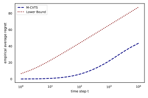
α=10%𝛼percent10\alpha=10\%
Refer to caption
Figure 8: Experiment 1 with Multinomial arms,
regret of M-CVTS and lower bound (abscissa log scale)
α=90%𝛼percent90\alpha=90\%

G.1.2 Experiments on general Bounded distributions: Truncated Gaussian Mixtures

In this section we consider bounded multi-modal distributions, built by truncated Gaussian Mixture models in [0,1]01[0,1]. We simply call these distributions Truncated Gaussian Mixtures (TGM for short). We first remark that these distributions are not continuous because they can have a positive mass in 00 and 111, but it is still a good illustrative example to check the performance of B-CVTS. Indeed, we also performed the same exact experiments making the distributions continuous (instead of truncating, we re-sampled observations until they lied in [0,1]01[0,1]) and the results were deemed to be exactly the same.

Continuous Experiments 1 to 4: Bi-modal Gaussian mixtures

We first consider experiments with two modes, each mode being equiprobable and having the same variance for simplicity (σ=0.1𝜎0.1\sigma=0.1) in all experiments. It is interesting to compare settings where some arms have modes that are both close to 0.50.50.5, and where other arms have a large mass of probability close to the two support bounds (one mode close to 111 and one close to 00).

We experiment 4 possible configurations of the modes, given by:

  • μ1=(0.2,0.5)subscript𝜇10.20.5\mu_{1}=(0.2,0.5)

  • μ2=(0,1)subscript𝜇201\mu_{2}=(0,1)

  • μ3=(0.3,0.6)subscript𝜇30.30.6\mu_{3}=(0.3,0.6)

  • μ4=(0.1,0.65)subscript𝜇40.10.65\mu_{4}=(0.1,0.65)

We indifferently call the arms by their means (saying arm μ1subscript𝜇1\mu_{1} for the TGM arm with the parameter μ1subscript𝜇1\mu_{1} along with the parameters we fixed).

As for the discrete setup in the previous section, we highlight some basic properties of their CVaRs: the distribution with parameter μ2subscript𝜇2\mu_{2} has a larger mean than the one with μ1subscript𝜇1\mu_{1}, but the 50%percent5050\% CVaR of μ1subscript𝜇1\mu_{1} is larger. We represented the CVaR for each parameter for different values of α(0,1]𝛼01\alpha\in(0,1] in Figure 9, with the thresholds α{0%,10%,90%}𝛼percent0percent10percent90\alpha\in\{0\%,10\%,90\%\} represented by the vertical lines. Interestingly, with these arms the most difficult problems are not necessarily those with smallest values of α𝛼\alpha. Indeed, for α=80%𝛼percent80\alpha=80\% it may be particularly difficult to choose between μ2subscript𝜇2\mu_{2} and μ3subscript𝜇3\mu_{3}, or between μ1subscript𝜇1\mu_{1} and μ4subscript𝜇4\mu_{4}, while μ3subscript𝜇3\mu_{3} is the clear winner for α=10%𝛼percent10\alpha=10\% due to the distribution being very concentrated around 0.50.50.5. Furthermore, the distribution μ2subscript𝜇2\mu_{2} is very concentrated around the bounds of the support but has a larger mean than the others, hence it becomes the best arm for values of α𝛼\alpha that are close to 111.

Refer to caption
Figure 9: CVaR of each TGM distribution νisubscript𝜈𝑖\nu_{i} (with centers μisubscript𝜇𝑖\mu_{i}), i=1,,4𝑖14i=1,\dots,4 for different values of α𝛼\alpha

We run the algorithms for α=10%,50%𝛼percent10percent50\alpha=10\%,50\% and 90%percent9090\% on four bandit problems with the following respective distributions:

  • ν1=(μ1,μ2)subscript𝜈1subscript𝜇1subscript𝜇2\nu_{1}=(\mu_{1},\mu_{2})

  • ν2=(μ1,μ3)subscript𝜈2subscript𝜇1subscript𝜇3\nu_{2}=(\mu_{1},\mu_{3})

  • ν3=(μ1,μ4)subscript𝜈3subscript𝜇1subscript𝜇4\nu_{3}=(\mu_{1},\mu_{4})

  • ν4=(μi)i{1,2,3,4}subscript𝜈4subscriptsubscript𝜇𝑖𝑖1234\nu_{4}=(\mu_{i})_{i\in\{1,2,3,4\}}

Results

In Tables 9,  1011 and  12 we report the results for the four considered problems (mean regret and standard deviation at T=10000𝑇10000T=10000). We also provide the regret curves, as for multinomial distributions, in order to check the logarithmic order of the regret of B-CVTS and its rate when T𝑇T is large.

Table 9: Results for TGM Experiment 1 at T=10000𝑇10000T=10000 for 5000 replications. Standard deviations in parenthesis.
α𝛼\alpha U-UCB CVaR-UCB B-CVTS
10%percent1010\% 274.9 (1.8) 5.3 (1.5) 1.1 (0.5)
50%percent5050\% 127.0 (19.3) 135.3 (41.1) 29.8 (17.2)
90%percent9090\% 80.5 (10.4) 53.5 (6.7) 10.2 (17.9)
Table 10: Results for TGM Experiment 2 at T=10000𝑇10000T=10000 for 5000 replications.
α𝛼\alpha U-UCB CVaR-UCB B-CVTS
10%percent1010\% 373.7 (4.1) 72.8 (9.6) 4.1 (2.3)
50%percent5050\% 135.8 (8.9) 37.9 (7.5) 5.5 (2.7)
90%percent9090\% 62.6 (7.1) 43.9 (5.1) 5.0 (1.8)
Table 11: Results for TGM Experiment 3 at T=10000𝑇10000T=10000 for 5000 replications.
α𝛼\alpha U-UCB CVaR-UCB B-CVTS
10%percent1010\% 269.4 (1.8) 23.2 (4.8) 2.8 (1.5)
50%percent5050\% 138.5 (12.4) 71.8 (19.0) 14.7 (8.3)
90%percent9090\% 53.1 (6.6) 34.5 (6.6) 20.2 (22.4)
Table 12: Results for TGM Experiment 4 at T=10000𝑇10000T=10000 for 5000 replications.
α𝛼\alpha U-UCB CVaR-UCB B-CVTS
10%percent1010\% 958.9 (4.8) 230.5 (25.3) 10.4 (3.2)
50%percent5050\% 318.4 (12.2) 147.7 (17.9) 21.2 (6.4)
90%percent9090\% 154.3 (11.9) 119.5 (11.7) 25.1 (14.1)

Again, the TS approach significantly outperforms the two UCB algorithms, which is a very interesting result: contrarily to the multinomial case, this time the three algorithms had the same level of information on arms’ distributions. B-CVTS is consistently the best for all four problems we implemented and for all α𝛼\alpha levels.

Continuous Experiment 5: Robustness to small α𝛼\alpha

We then check the robustness of B-CVTS to a smaller value of the parameter α𝛼\alpha by setting α=1%𝛼percent1\alpha=1\%, referred as Experiment 5. The bandit of Experiment 5 has six TGM arms with respective mean and variance parameters μ135=(0.3,0.6)subscript𝜇1350.30.6\mu_{135}=(0.3,0.6), μ246=(0.25,0.65)subscript𝜇2460.250.65\mu_{246}=(0.25,0.65), σ12=0.05subscript𝜎120.05\sigma_{12}=0.05, σ34=0.06subscript𝜎340.06\sigma_{34}=0.06, σ56=0.07subscript𝜎560.07\sigma_{56}=0.07. This experiment allows to additionally check if adding different variances to the arms affects the performance of the algorithms. However, we keep the probability of each mode to 0.50.50.5. This problem provides the following CVaR values for each arm at level 1%percent11\%, respectively: c1:60.01=[0.18,0.13,0.15,0.10,0.13,0.08]subscriptsuperscript𝑐0.01:160.180.130.150.100.130.08c^{0.01}_{1:6}=[0.18,0.13,0.15,0.10,0.13,0.08]. The results are reported in Table 13, in which we observe a very large performance gap between B-CVTS and UCB algorithms. This is particularly interesting because it shows that the UCB algorithms are not really able to learn for very small values of α𝛼\alpha (indeed α=1%𝛼percent1\alpha=1\% is very small when drawing only a total number of 104superscript10410^{4} observations) before the horizon becomes extremely large. We already observed this behavior for CVaR-UCB in previous experiments, but this time we can see as well that its average regret is even higher than the one of U-UCB, and its variance spiked. On the other hand, B-CVTS seems to learn smoothly even for α=1%𝛼percent1\alpha=1\%, as its average regret only doubles between T=1000𝑇1000T=1000 and T=5000𝑇5000T=5000, and increases even less between T=5000𝑇5000T=5000 and T=10000𝑇10000T=10000.

Table 13: Results for TGM Experiment 5 (α=1%𝛼percent1\alpha=1\%) at T=10000𝑇10000T=10000 for 5000 replications.
T U-UCB CVaR-UCB B-CVTS
1000 49.1 (0.3) 53.2 (5.6) 18 (37)
5000 245 (1.1) 263.2 (24.7) 35.5 (51)
10000 489.1 (2.2) 518.4 (45.0) 41 (66)
Table 14: Results for TGM Experiment 6, at T=10000𝑇10000T=10000 averaged over 400 random instances with K=30𝐾30K=30 truncated Gaussian mixtures with 10 modes.
T U-UCB CVaR-UCB B-CVTS
10000 2149.9 (263) 2016.0 (265) 210.9 (6.4)
20000 4276.4 (538) 3781.3 (521) 237.1 (15.4)
40000 8493.4 (1085) 6894.1 (985) 263.5 (17.9)
Continuous Experiment 6: Random Problems with more modes and more arms

Finally, we further check the robustness of B-CVTS to more arms and more diverse distribution profiles by increasing the number of possible modes. To do so, we implement an experiment with K=30𝐾30K=30 arms, with TGM distributions with 10 modes exhibiting different means and variances, which covers a large variety of shapes of distributions. All of those parameters are drawn uniformly at random, and we summarize their distributions as (μ,σ)𝒰([0.25,1]10×[0,0.1]10)similar-to𝜇𝜎𝒰superscript0.25110superscript00.110(\mu,\sigma)\sim\mathcal{U}([0.25,1]^{10}\times[0,0.1]^{10}), and p𝒟10similar-to𝑝subscript𝒟10p\sim\mathcal{D}_{10} (uniform distribution on the simplex, presented in Section 3). We name this setting TGM Experiment 6. The results of this experiment are reported in Table 14 for a parameter α=0.05𝛼0.05\alpha=0.05 averaged over 400 random instances. Again, we choose a smaller value for α𝛼\alpha than in the previous extensive sets of experiments because problems with small α𝛼\alpha seem to be more challenging. The results highlight that best performances are obtained by B-CVTS.

Conclusions

We preliminary evaluated the CVaR bandit algorithms on synthetic problems before testing them on realistic-world bandit environment in the next section. These experiments seem to highlight a greater robustness of B-CVTS to many different settings regarding different parameters: α𝛼\alpha level, the number of arms K𝐾K and the different possible shapes of the distributions (symbolized by the number of modes in our synthetic experiments). In particular, B-CVTS is the only algorithm that has not shown to be affected by the value of α𝛼\alpha, as the two UCB algorithms had their respective performances degraded in some extent depending on α𝛼\alpha values.

G.2 Experiments with DSSAT crop-model

In this section we keep comparing  B-CVTS  with U-UCB and CVaR-UCB for α{5%,10%,80%}𝛼percent5percent10percent80\alpha\in\{5\%,10\%,80\%\} as described in section 4. DSSAT is still parameterized with the same challenging conditions, but we generate two different problems thanks to the crop-simulator. For both presented experiments we consider N=1040𝑁1040N=1040 runs of each algorithm up to a time horizon T=10000𝑇10000T=10000. As explained in section 4, all DSSAT arms’ distributions are empirically estimated from 106superscript10610^{6} samples in both experiments.

DSSAT Experiment 1: 7 armed planting date bandit

We consider a bandit instance that consists of 7 arms, each arm corresponds to a planting date spaced of 15 days from the previous one. An illustration of the underlying distributions is given in Figure 10. In this case, the best arm is consistent with all values of α𝛼\alpha, as shown in Table 16. Nevertheless, arms exhibit different gaps when considering different values of α𝛼\alpha. This experiment intends to evaluate B-CVTS robustness for a greater number of real-world alike arms with a diversity of reward distribution shapes.

The results of this experiment are reported in Table 18. The regret curves for the three algorithms, with considered values of α𝛼\alpha parameter are illustrated in Figures 1214, and  16.

In this experiment, by exhibiting superior performances  B-CVTS  appears to be more robust than the UCB CVaR bandit algorithms relative to an increase in the number of arms. In practice for the planting-date problem, a global, few months planting-window is known but needs further refinements e.g. to identify the best two-week time slot for planting. That is to say, the number of arms is unlikely to be greater that what has been tested in this experiment, making B-CVTS a particularly fit-for-purpose candidate in this setup.

DSSAT Experiment 2: Impact of support upper bound over-estimation

This configuration is the same than the one presented in Section  4, but here we largely over-estimate the yield upper-bound to 30 t/ha, when a close to reality yield upper bound is about 10 t/ha. From an agronomic point of view, this yield value is a very unlikely over-estimation in the given conditions. This experiment intends to empirically evaluate how a rough arms’ upper-bound estimation affects algorithms’ performances, when little expert knowledge is available. An illustration of the underlying distributions and how the upper-bound estimation is exaggerated is given in Figure 11 and corresponding metrics are reported in Table 16.

We provide the results of this experiment in Table 18, and display the regret curves in Figures 1315, and  17.

Experiment 2 addresses one possible concern for practitioners: the prerequisite of rewards’ support upper bound. We empirically demonstrate that with realistic simulations, when a highly over-estimated, unrealistic support upper-bound is given – triple of expert’s estimation –, B-CVTS  keeps outperforming UCB-like CVaR bandit algorithms. We shown that this over-estimation did not affect  B-CVTS  performances compared to the situation of correct support upper-bound identification as presented in Section 4. In particular, it even slightly improved its performance for α=80%𝛼percent80\alpha=80\%. This result is counter-intuitive, but it can be explained by the fact that the extra exploration induced by the larger upper bound may have sped up learning in this particular case, improving overall performances. On the other hand, CVaR-UCB seems much more impacted by this over-estimation (regret is respectively increased by about 150%percent150150\%, 75%percent7575\% and 78%percent7878\% for α{5%,20%,80%}𝛼percent5percent20percent80\alpha\in\{5\%,20\%,80\%\}). Similarly U-UCB shown altered performances, despite its already unsatisfying results when considering the true upper bound.

Conclusions

B-CVTS  appeared to be a satisfying candidate for real-world alike problems, as shown with the planting date bandits. We empirically showed the  B-CVTS  was best able to deal with a greater number of planting date arms than its UCB counterparts. We showed as well that B-CVTS  remained the best performer despite considering a very unlikely support upper-bound estimation. We think that in many physical resource-based problems, this should be reassuring for practitioners, in particular when compared with UCB algorithms’ sensibility to the input upper bound.
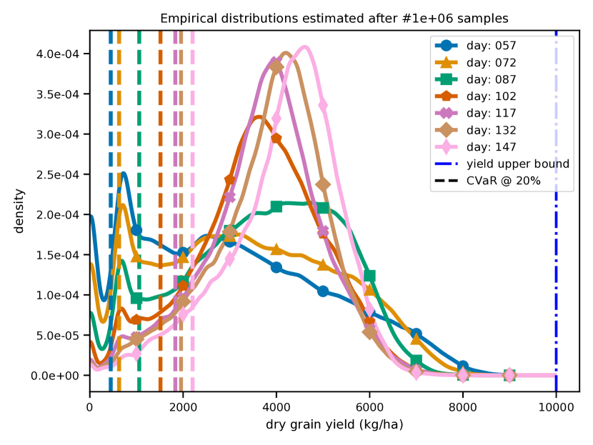
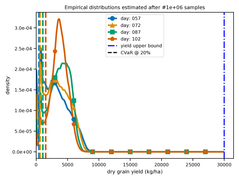
Refer to caption
Figure 10: Experiment 1, 7 armed DSSAT environment empirical distributions ; 106superscript10610^{6} samples.
Refer to caption
Figure 11: Experiment 2, 4 armed DSSAT environment empirical distributions with over-estimated support ; 106superscript10610^{6} samples.
Table 15: DSSAT Experiment 1 distribution metrics in kg/ha estimated from 106superscript10610^{6} samples..
day (action) CVaRαsubscriptCVaR𝛼\text{CVaR}_{\alpha}
5%percent55\% 20%percent2020\% 80%percent8080\% 100%percent100100\% (mean)
057 0 448 2238 3016
072 46 627 2570 3273
087 287 1059 3074 3629
102 538 1515 3120 3586
117 808 1832 3299 3716
132 929 1955 3464 3850
147 1122 2203 3745 4112
Table 16: DSSAT Experiment 2 distribution metrics in kg/ha estimated from 106superscript10610^{6} samples.
day (action) CVaRαsubscriptCVaR𝛼\text{CVaR}_{\alpha}
5%percent55\% 20%percent2020\% 80%percent8080\% 100%percent100100\% (mean)
057 0 448 2238 3016
072 46 627 2570 3273
087 287 1059 3074 3629
102 538 1515 3120 3586
Table 17: Results for DSSAT Experiment 1, empirical regret at T=10000𝑇10000T=10000 in t/ha for 1040 replications. Standard deviations in parenthesis.
α𝛼\alpha U-UCB CVaR-UCB B-CVTS
5%percent55\% 5687 (5) 1891 (18) 700 (22)
20%percent2020\% 6445 (10) 1795 (19) 489 (17)
80%percent8080\% 3367 (14) 1580 (15) 293 (8)
Table 18: Results for DSSAT Experiment 2, empirical regret at T=10000𝑇10000T=10000 in t/ha for 1040 replications.
α𝛼\alpha U-UCB CVaR-UCB B-CVTS
5%percent55\% 3179 (2) 759 (14) 195 (11)
20%percent2020\% 5644 (6) 1020 (17) 202 (10)
80%percent8080\% 2642 (10) 888 (13) 284 (12)
Refer to caption
Figure 12: DSSAT Experiment 1, 7 armed bandit
all algorithms, α=5%𝛼percent5\alpha=5\% ; 1040 replications.
Refer to caption
Figure 13: DSSAT Experiment 2,
4 armed over-estimated support upper bound,
all algorithms, α=5%𝛼percent5\alpha=5\% ; 1040 replications.
Refer to caption
Figure 14: DSSAT Experiment 1,
all algorithms, α=20%𝛼percent20\alpha=20\%
Refer to caption
Figure 15: DSSAT Experiment 2,
all algorithms, α=20%𝛼percent20\alpha=20\%
Refer to caption
Figure 16: DSSAT Experiment 1,
all algorithms, α=80%𝛼percent80\alpha=80\%
Refer to caption
Figure 17: DSSAT Experiment 2,
all algorithms, α=80%𝛼percent80\alpha=80\%