Adaptive Single- and Multilevel Stochastic Collocation Methods for Uncertain Gas Transport in Large-Scale Networks
Abstract
In this paper, we are concerned with the quantification of uncertainties that arise from intra-day oscillations in the demand for natural gas transported through large-scale networks. The short-term transient dynamics of the gas flow is modelled by a hierarchy of hyperbolic systems of balance laws based on the isentropic Euler equations. We extend a novel adaptive strategy for solving elliptic PDEs with random data, recently proposed and analysed by Lang, Scheichl, and Silvester [J. Comput. Phys., 419:109692, 2020], to uncertain gas transport problems. Sample-dependent adaptive meshes and a model refinement in the physical space is combined with adaptive anisotropic sparse Smolyak grids in the stochastic space. A single-level approach which balances the discretization errors of the physical and stochastic approximations and a multilevel approach which additionally minimizes the computational costs are considered. Two examples taken from a public gas library demonstrate the reliability of the error control of expectations calculated from random quantities of interest, and the further use of stochastic interpolants to, e.g., approximate probability density functions of minimum and maximum pressure values at the exits of the network.
1 Introduction
The role of natural gas transport through large-scale networks has been rapidly increased through the ongoing replacement of traditional energy production by coal fired and nuclear plants with gas consuming facilities. The safekeeping of energy security and the development of clean energy to meet environmental demands have generated a significant increase in gas consumption for electric power stations in the last decade. The future energy mix will mainly be based on low-carbon and regenerative energy and natural gas is considered as a bridging combustible resource to achieve this goal. The seasonally fluctuating disposability of wind and solar resources causes a growing variability in electricity production and hence also in the demands of gas transportation by pipelines. The resulting intra-day uncertain oscillations in demand for natural gas leads to new challenges for computer based modelling and control of gas pipeline operations. Here, an increasing focus lies on the short-term transient dynamics of gas flow. Operators have to responsively control varying loads to realize a reliable operational management for both gas and electricity delivery systems. These challenging new conditions demand advanced decision tools based on reliable transient simulation and uncertainty quantification taking into account serious operating restrictions.
In this paper, we propose a novel computational approach for the reliable quantification of the transport of uncertainties through a network of gas pipelines. It extends an adaptive multilevel stochastic collocation method recently developed in [22] for elliptic partial differential equations with random data to systems of hyperbolic balance laws with uncertain initial and boundary conditions. We have been developing in-house software tools for fast and reliable transient simulation and continuous optimization of large-scale gas networks over the last decade [7, 8, 9, 10, 11]. Exemplarily, here we will investigate the important task of safely driving a stationary running system into a newly desired system defined by uncertain gas nominations at delivery points of the network. To be usable in a real-time application of risk analysis and reliability assessment of gas delivery, we have designed our method to meet user-defined accuracies while keeping the computing time for large-scale gas networks at a moderate level. It offers also the opportunity to be integrated in a probabilistic constrained optimization approach [30].
We will consider the following one-dimensional parameterized hyperbolic system of balance laws on a set of gas pipes , , with random initial and boundary data:
| (1) | |||||
| (2) | |||||
| (3) | |||||
| (4) |
where the solutions are represented as with the deterministic physical domain and being a stochastic parameter space of finite dimension (finite noise assumption). The component parameters will be associated with independent random variables that have a joint probability density function such that . Typically, gas pipeline systems are buried underground and hence temperature differences between a pipe segment and the ground can be neglected in practice. It is therefore standard to consider an isothermal process without a conservation law for the energy, i.e., is the vector of density and momentum for each pipe with being the velocity.
The index sets and in (3) and (4) describe the indices of the boundary and the coupling nodes, respectively. Boundaries in gas networks are sources, where gas is injected into the pipeline system, and exits, where it is taken out by consumers. The modelling of connected pipes, flow at junctions, and the pressure increase caused by a compressor leads to certain coupling conditions in (4) at inner nodes. We ensure conservation of mass and claim the equality of pressure, except for compressors, where the time-dependent term represents the pressure jump that is realised by the compression process. The pressure is calculated from the equation of state for real gases, , with compressibility factor .
We also allow for different gas transport models in each pipe. They are identified by the parameters in (1) representing a whole hierarchy of models with decreasing fidelity. In our applications, we use the nonlinear isothermal Euler equations as , its semilinear approximation as , and a quasi-stationary model as . They will be described in more detail later on.
Let and . Throughout this paper, we assume that there is a unique weak entropy solution of the gas flow problem (1)-(4) for all . For uncertainty quantification in gas network applications, it is more natural to consider a functional of the solution instead of the solution itself. Thus, suppose a possibly nonlinear functional (or quantity of interest) with is given. The standard collocation method is based on a set of deterministic sample points in , chosen to compute independent, finite dimensional space-time approximations . These approximations are used to construct a single-level interpolant
| (5) |
for the function in the polynomial space with basis functions ,
| (6) |
The interpolation conditions for determine the coefficients . The quality of the interpolation process depends on the accuracy of the space-time approximations , the regularity of the solution with respect to the stochastic parameters , and on the number of collocation points , which grows rapidly with increasing stochastic dimension . The interpolant , also called response surface approximation, can be used to directly calculate moments such as expectation and variance. Since its evaluation is extremely cheap, it also forms the basis for approximating its probability density function by a kernel density estimator and determining the practically relevant probability that lies in a certain interval over the whole time horizon. We will apply this approach to check the validity that gas is delivered in a pressure range stipulated in a contract between gas company and consumer.
The uncertainties in the initial and boundary data in (2) and (3) result in a propagation of uncertainties in the functional . It is essential in nowadays natural gas transport through large networks that operators apply a reliable operational management to guarantee a sufficiently smooth gas flow, respecting at the same time operating limits of compressors and pressure constraints inside the pipes in a safe manner. There is always a safety factor that prevents the whole transport system to really hit the limits. Therefore, we may assume appropriate regularity of the solution in the random space in order to ensure a fast convergence of the global approximation polynomials in (5). Exemplarily, we will investigate the influence of uncertain gas demand when safely driving a stationary running system into a newly desired system defined by shifted gas nominations at the delivery points of the network.
There are two main alternative approaches to stochastic collocation: Monte Carlo sampling and stochastic Galerkin methods. A detailed discussion of comparative advantages and disadvantages in the context of hyperbolic systems of conservation laws is given in [2], see also [5, 14] for a general overview on uncertainty quantification in solutions of more general partial differential equations. Monte Carlo methods and its variants are the most commonly used sampling methods. They are non-intrusive and robust with respect to lack of regularity, have a dimension-independent convergence rate and offer a trivial parallelization. However, they are not able to exploit any smoothness or special structure in the parameter dependence and their convergence rate is rather low even when Multilevel Monte Carlo methods are applied. Combined with finite volume discretizations for the physical space, such methods are extensively investigated in [25, 26, 27]. Stochastic Galerkin methods based on generalized polynomial chaos are intrusive and request the solution of heavily extended systems of conservation laws [28, 33]. Although sparse grids and efficient solvers for block-structured linear systems are used, the computational costs in general are formidable. Recently, an intrusive polynomial moment method which is competitive with non-intrusive collocation methods has been proposed in [21]. In the presence of discontinuities in the random space, promising semi-intrusive approaches are provided by the stochastic finite volume method [1] and a novel hierarchical basis weighted essentially non-oscillatory interpolation method [19].
The paper is organised as follows. In section 2, we describe the single-level approach and especially focus on the main ingredients for the adaptive solvers in the physical and parameter space. The extension to the multilevel approach is explained in section 3, where we also give asymptotic rates for the complexity of the algorithm. In section 4, two examples based on networks from a public gas library are investigated to demonstrate the efficiency and potential of the fully adaptive collocation method. We conclude with a summary and outlook in section 5.
2 Adaptive Single-Level Approach
The main advantage of sampling methods is the reuse of an efficient solver for the transient gas flow through a network in the range of parameters defined by the stochastic space . Since the gas transport through a complex network may be very dynamic and thus changes both in space and time, an automatic control of the accuracy of the simulation is mandatory. In order to further reduce computational costs, adjusting the transport model in each pipe according to the time-dependent dynamics has proven to be very attractive. As a rule of thumb, the most complex nonlinear Euler equations () should be used when needed and the simplest algebraic model () should be taken whenever possible without loosing too much accuracy. In a series of papers, we have developed a posteriori error estimates and an overall control strategy to reduce model and discretization errors up to a user-given tolerance [7, 8, 9, 10, 11]. A brief introduction will be given next.
Let a parameter be fixed and an initial distribution of gas transport models be given. Then, we solve the gas network equations (1)-(4) by means of an adaptive implicit finite volume discretization [20] applied for each pipe until the estimate of the error in the functional is less than a prescribed tolerance . Here, refers to resolution in space, time and model hierarchy. To raise efficiency, the simulation time is divided into subintervals , , of the same size. We then successively process the classical adaption loop
| (7) |
for each of the subintervals such that eventually
| (8) |
in the second step with a sample-dependent constant that is usually close to one. The a posteriori error estimators , , and for the -th pipe determine the error distribution along the network for the spatial, temporal and model discretizations. They measure the influence of the model and the discretisation on the output functional and can be calculated by using the solutions of adjoint equations. A detailed description which would go beyond the scope of our paper is given in [7, Sect. 2.2], see also [9, 10]. Polynomial reconstructions in space and time of appropriate orders are used to compute and , respectively. The model error estimator is derived from the product of differential terms, representing the difference between models, and the sensitivities calculated from the adjoint equations.
In our calculations, we use the following model hierarchy:
-
•
: Nonlinear isothermal Euler equations
-
•
: Semilinear isothermal Euler equations
-
•
: Algebraic isothermal Euler equations
with the joint source term , where is the pipe diameter and the Darcy friction coefficient. We note that the algebraic model can be analytically solved in the variables and . The models are connected at inner nodes, where we ensure conservation of mass and the equality of pressure. The latter one is often used in engineering software, but can be also replaced by the equality of total enthalpy. The interested reader is referred to the discussion in [24]. Pipes can also be connected by valves and compressors. Valves are used to regulate the flow in gas networks. An open valve is modelled as inner node, whereas is required at both sides of a closed valve. Compressors compensate for the pressure loss due to friction in the pipes. The power of a compressor that is needed for the compression process is given by
| (9) |
with in- and outgoing pressure , , and ingoing flow rate [23]. The parameter is a compressor specific constant, the isentropic coefficient of the gas, and the compressibility factor from the equation of state for real gases. In our application, we use the specific energy consumption needed by the electric motors to realize all desired compressions as quantity of interest that drives the adaptation process. It can be estimated by a quadratic polynomial in , i.e., we set
| (10) |
with given compressor-dependent constants and a scaling factor .
The complex task in the step MARK (for refinement) of finding an optimal refinement strategy that combines the three types of adaptivity is a generalisation of the unbounded knapsack problem, which is NP-hard. A good approximation can be found by a greedy-like refinement strategy as investigated in [7]. It leads to considerable computational savings without compromising on the simulation accuracy. Eventually, we have an adaptive black box solver - our working horse - at hand that, once a random parameter and a specific tolerance have been chosen, delivers a numerical approximation such that the accuracy requirement (8) is satisfied for
| (11) |
Working close to the asymptotic regime, we can assume that the adaptive algorithm converges for fixed and .
Starting from the pointwise error estimate (8) and supposing bounded first moments of , we directly get the following error bound:
| (12) |
with a constant
| (13) |
that does not depend on .
We will now discuss the control of the error for the adaptive stochastic collocation method. Let us assume and consider the interpolation operator from (5). This operator is constructed by a hierarchical sequence of one-dimensional Lagrange interpolation operators, using the anisotropic Smolyak algorithm as introduced in [13]. It reads
| (14) |
with multi-indices , , and univariate polynomial interpolation operators . These operators use collocation points to construct a polynomial interpolant in of degree at most . The operators are often referred to as hierarchical surplus operators. The function has to satisfy , , and . We formally set for all and use the nested sequence of univariate Clenshaw–Curtis nodes with if . The index in (14) is then the number of all explored quadrature points in determined by .
The value of the hierarchical surplus operator in (14) can be interpreted as profit and therefore used as error indicator for already computed approximations. Applying once again the classical adaption loop from (7), the adaptive anisotropic Smolyak algorithm computes profits in each step, adds the index of the highest profit to the index set and explores admissible neighbouring indices next. The algorithm stops if the absolute value of the highest profit is less than a prescribed tolerance, say . Obviously, the method is dimension adaptive. There is a Matlab implementation Sparse Grid Kit available, which can be downloaded from the CSQI website [4]. Its numerical performance is discussed in the review paper [31].
Following this adaptive methodology, we get an error estimate
| (15) |
with a constant . We assume that does not depend on . If we now split the overall error into the sum of a physical error resulting from the chosen resolution in space, time and model hierarchy, and a stochastic interpolation error, then using the inequalities (12), (15) and the triangle inequality yields the final estimate
| (16) |
Let be a user-prescribed tolerance for the error on the left-hand side. Then the usual strategy to balance both the physical and the stochastic error on the right-hand side is to choose the individual tolerances as and . Finally, the adaptive Smolyak algorithm is called with the tolerance , where for each chosen sample point , the black box solver in (11) runs with ANet(), resulting in a sample-adaptive resolution in the physical space. The algorithm is illustrated in Tab. 1.
| Algorithm: Adaptive Single-Level Stochastic Collocation Method | |
|---|---|
| 1. | Given , estimate , , and set , . |
| 2. | Compute := ASmol(ANet(),). |
3 Adaptive Multilevel Approach
Next, we consider an adaptive multilevel approach in order to enhance the efficiency of the uncertainty quantification further. First multilevel strategies in the context of Monte Carlo methods were independently proposed as an abstract variance reduction technique in [15, 17]. Extensions to uncertainty quantification were developed in [3, 6]. Later on, they also entered the field of stochastic collocation methods [22, 32, 34]. The methodology in this paper can be viewed as an extension of the adaptive multilevel stochastic collocation method developed for elliptic PDEs with random data in [22] to the hyperbolic case, where a sample-dependent hierarchy of spatial approximations is replaced by a more sophisticated space-time-model hierarchy.
Let a sequence of tolerances with
| (17) |
be given. Each refers to a certain resolution in space, time and model hierarchy such that for any solution with it holds
| (18) |
with a constant that does not depend on . The constants are defined in (13) with . We consider now a second family of (stochastic) tolerances and assume that there exits numbers , and a positive constant not depending on such that
| (19) |
for . Here, we formally set . Observe that with increasing index , the differences decrease and hence the number of collocation points necessary to achieve the tolerance gets smaller. Consequently, less samples on fine meshes and with high fidelity models are needed to achieve the overall tolerance, which is the main motivation for the use of a multilevel approach.
Using a telescopic sum of single-level interpolants, we construct a multilevel interpolant for the functional through
| (20) |
Its error can be estimated by
| (21) |
where we have used the identity and the inequalities (18) and (19). There are two different ways to balance the errors on the right-hand side: (1) set for all , which yields as upper bound in (16), and (2) choose in such a way that the computational cost is minimized. We will go for the second option and follow the suggestions given in [22]. Let denote the work (computational cost) that must be invested to solve the gas network equations for a sample point with accuracy . Then we make the following assumptions:
| (22) |
for all . Here, we fix . The constants , are independent of , , and the rates and are strictly positive. Recall that is the dimension of the stochastic space.
To achieve an accuracy for the multilevel interpolant, i.e.,
| (23) |
at minimal cost , the optimal choice of the stochastic tolerances is given in [22, Theorem 2.1]. They are
| (24) |
where
| (25) |
Typically, in practical calculations, a decreasing sequence of tolerances with a positive reduction factor is used. In this case, we can estimate the overall multilevel costs using a standard construction [22, Theorem 2.2],
| (26) |
| Algorithm: Adaptive Multilevel Stochastic Collocation Method | |
|---|---|
| 1. | Given , , and , estimate , , , and set . |
| 2. | Set for . |
| 3. | Compute := ASmol(ANet(),). |
| 4. | Set for . |
| 5. | Compute := ASmol(ANet(),). |
| 6. | Compute := ASmol(ANet() - ANet(),) for . |
| 7. | Compute . |
For the convenience of the reader, we summarize the multilevel algorithm in Table 2. Once the parameters are set, the approach is self-adaptive in nature. Observe that already computed samples at level can be reused to compute in step 6. In general, sufficient estimates for the constants , and the rates , can be derived from the study of a few samples with relatively coarse resolutions. In any case, these samples can be reused later on.
4 Practical Examples from a Gas Library
Examplarily, we will consider two gas network configurations: GasLib-11 and GasLib-40 from the public gas library gaslib.zib.de [29]. They are parts of real gas networks in Germany. We have implemented the adaptive approach described above for the deterministic black box solver ANet() from (11) in our in-house software package Anaconda. More details of the implementation can be found in [18]. The adaptive stochastic collocation method ASmol() was realized by means of the Sparse Grid Kit developed in Matlab [31]. All calculations have been done with Matlab version R2020a on a Intel(R) Xeon(R) Gold 6130 CPU running at 2.1 GHz.
A common daily operation of gas networks is the smooth transformation of a stationary state , which has worked well for the given demands so far, into a new stationary state , which realizes a change in the gas demand over a couple of hours. This scenario is best treated by appropriate optimization tools which determine the operating range of all compressor stations and valves in such a way that, e.g., lower and upper bounds of pressures are satisfied during the whole time-dependent conversion process. In what follows, we will assume that a feasible, optimized control, i.e., the operation modes for compressors (pressure jump) and valves (open or closed), is already known for this so-called nomination change. Then, we will fix these controls and focus on the influence of uncertainties in the consumers’ demands around state on the compressor costs and the feasibility of the pressure at which the gas is delivered to the consumers. Typically, corresponding pressure requirements are regulated in contracts.
4.1 An Example with 11 Pipes
The first example is taken from the GasLib-11, which consists of pipes, compressors, valve, sources, and exits, see Fig. 1. The stationary initial state and the final state are determined by the boundary conditions and controls given in Tab. 3. The simulation is started with . After , the boundary values and controls are linearly changed to reach the new conditions defined for at . The valve is closed at . The simulation time of is split into subintervals of , for which the classical adaption loop (7) is processed.
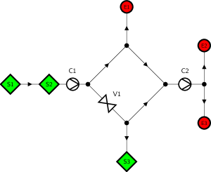
| State | State | |||||
| source | S1 | S2 | S3 | S1 | S2 | S3 |
| pressure [] | 70.00 | 70.00 | 65.00 | 48.00 | 54.00 | 46.00 |
| exit | E1 | E2 | E3 | E1 | E2 | E3 |
| volume flow [] | 38.22 | 38.22 | 38.22 | 25.48 | 25.48 | 25.48 |
| compressor | C1 | C2 | C1 | C2 | ||
| pressure jump [] | 0 | 0 | 5 | 15 | ||
| valve | V1 | V1 | ||||
| operation | open | closed | ||||
For the state , the volume flows at the three exists , are uncertain due to an individual behaviour of the consumers and are parameterised by three variables , representing the image of a triple of independent random variables with . We set
| (27) |
According to (10), the quantity of interest is defined by the specific energy consumption of the compressors,
| (28) |
with , , for both compressors and defined in (9). We set the weighting factor to bring the expected value of in the order of .
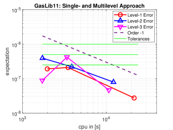
In order to start the adaptive stochastic collocation method, we have performed a few calculations for low tolerances to estimate the parameters in Tab. 2. We found , , and by a least squares fit and appropriate rounding. Let us now consider a single-, two, and three-level approach with a reduction factor . The overall accuracy requirements are , where a reference solution is calculated with . The results are shown in Fig. 2. The differences of the methods are not very high. This is due to the fact that only collocation points are sufficient to reach the highest accuracy.
We can also use the anisotropic Smolyak decomposition in (14) to study the validity of the pressure bounds at the three exists , , and . Replacing by the time-dependent pressure yields
| (29) |
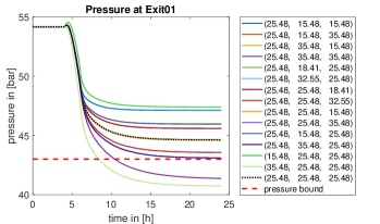
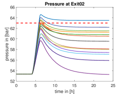
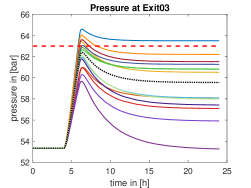
Exemplarily, in Fig. 3, we show the pressure curves at the exits for collocation points adaptively chosen by the Smolyak algorithm for . Supposing a feasible range for the pressure at which the gas should be delivered to the consumers, we are now interested in the probabilities
| (30) |
with and . The surrogate model (29) allows a fast evaluation over a sufficiently fine uniform mesh in the stochastic parameter space , thus giving enough information to approximate the probability density functions of the random variables and by a one-dimensional kernel density estimator (KDS)
| (31) |
for , where and . Observe that the bandwidth depends on the standard deviation of the samples as, e.g., stated and explained in [16, Chap. 4.2].
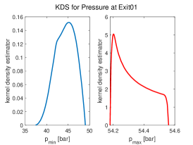
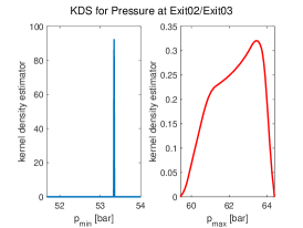
The corresponding KDSs are plotted in Fig. 4.
From the KDSs, we calculate
| (32) |
With such information at hand, a managing operator is prepared to react on sudden changes in the gas network with an appropriate adaptation of the controls. It also forms the basis for probabilistic constrained optimization, see [30] for more details.
4.2 An Example with 40 Pipes
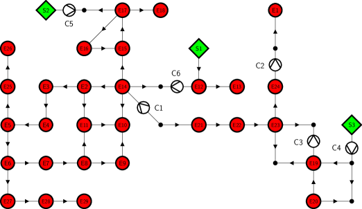
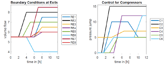
Our second example is GasLib-40, a simplified real part of the German Gas Network, and consists of pipes, compressor stations, sources, and exits. Its structure is shown in Fig. 5. The exits will be clustered in different local regions (REs) with equal uptake rates and uncertainties:
| (33) |
The stationary initial state and the final state are determined by the boundary conditions and controls given in Tab. 4. The temporal evolution of these values is shown in Fig. 6. The computational time interval is split into equal subintervals.
The quantity of interest is again defined by the specific energy consumption of the compressors,
| (34) |
with , , for all compressors and defined in (9). The weighting factor is chosen as to get values of moderate size, i.e., around .
First, we would like to demonstrate the performance of the adaptive black box solver ANet() for this larger network. Given the boundary conditions and controls defined in Fig. 6, we always start with the initial time step , the mesh width , and the simplest algebraic model . The statistics of the runs for tolerances are summarized in Tab. 5. The observed estimation process is quite reliable and the tolerances are always satisfied. It is nicely seen that the portion of the most detailed physical model is increasing with higher tolerances. For the last three tolerances, we can detect . This was also reported for even more complex networks in [12].
Next, we model uncertainties in the exit regions RE1-RE8 by eight independent, uniformly distributed parameters , , to describe random volume flows for the state through
| (35) |
where is the corresponding volume flow for the stationary state defined in Tab. 4. The parameters necessary to run the adaptive stochastic collocation methods were determined by a few samples for low tolerances as follows: , , , and .
| State | State | |||||||
| source | S1 | S2 | S3 | S1 | S2 | S3 | ||
| pressure [] | 60.0 | 53.2 | 53.2 | 60.0 | 58.0 | 53.2 | ||
| exit | RE1 | RE2 | RE3 | RE4 | RE1 | RE2 | RE3 | RE4 |
| volume flow [] | 5.5 | 5.5 | 5.5 | 5.5 | 7.5 | 8.0 | 6.5 | 6.0 |
| exit | RE5 | RE6 | RE7 | RE8 | RE5 | RE6 | RE7 | RE8 |
| volume flow [] | 5.5 | 5.5 | 5.5 | 5.5 | 7.0 | 4.0 | 8.5 | 6.0 |
| compressor | C1 | C2 | C3 | C4 | C1 | C2 | C3 | C4 |
| pressure jump [] | 0 | 0 | 5 | 0 | 5 | 15 | 7 | 12 |
| compressor | C5 | C6 | C5 | C6 | ||||
| pressure jump [] | 0 | 0 | 5 | 12 | ||||
| ERR | EST | CPU[s] | ||||
|---|---|---|---|---|---|---|
| 3600/1800 | 7915/767 | 0:0:100 | 3.1 | |||
| 3600/1800 | 7915/767 | 05:20:75 | 4.2 | |||
| 1800/1800 | 7915/767 | 17:51:32 | 5.3 | |||
| 112/112 | 7915/767 | 31:56:13 | 47.9 | |||
| - | 28/7 | 7807/767 | 46:47:07 | 511.5 |
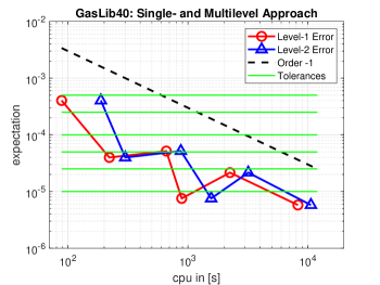
Let us now consider a single- and two-level approach with a reduction factor and tolerances . We computed a reference solution with . The results are shown in Fig. 7. Both methods deliver equal values for the expectation of . A closer inspection shows that only collocation points on the finest level are sufficient to reach the desired accuracy in all runs. This also explains the observation that the two-level approach takes slightly larger computing times since the method additionally calculates values on the coarse level. As also seen in the last example, the numbers of samples necessary to reach the tolerances are extremely small such that the single-level approach works already very efficient.
5 Conclusion and Outlook
In this study, we have applied a combination of two state-of-the-art adaptive methods to quantify smooth uncertainties in gas transport pipelines governed by systems of hyperbolic balance laws of Euler type. Our in-house software tool Anaconda and the open-source Matlab package Sparse Grid Kit provide a posteriori error estimates that can be exploited to drastically reduce the number of degrees of freedom by using a sample-dependent strategy so that the computational effort at each stochastic collocation point can be optimised individually. A single-level as well as a multilevel approach have been discussed and applied to two practical examples from the public gas library gaslib.zib.de. Both strategies perform similar and quite reliable even for very high levels of accuracy. However, we expect to see a greater potential of the multilevel approach when facing more challenging problems in future case studies.
In contrast to Monte Carlo methods, stochastic collocation schemes provide an access to a global interpolant over the parameter space, which can be interpreted as response surface approximation and used to easily calculate statistical moments and approximate probability density functions in a postprocessing. We are planning to incorporate these techniques into our continuous optimization framework and thus aiming for solving nonlinear probabilistic constrained optimization problems.
Acknowledgements. The authors are supported by the Deutsche Forschungsgemeinschaft (DFG, German Research Foundation) within the collaborative research center TRR154 “Mathematical modeling, simulation and optimisation using the example of gas networks“ (Project-ID239904186, TRR154/2-2018, TP B01). We would like to thank Oliver Harbeck for making his drawing software available to us. We have enjoyed using it to create the figures 1 and 5.
References
- [1] R. Abgrall and P. Congedo. A semi-intrusive deterministic approach to uncertainty quantification in non-linear fluid flow problems. J. Comput. Phys., 235:828–845, 2013.
- [2] R. Abgrall and S. Mishra. Chapter 19 - uncertainty quantification for hyperbolic systems of conservation laws. In R. Abgrall and C.-W. Shu, editors, Handbook of Numerical Methods for Hyperbolic Problems, volume 18 of Handbook of Numerical Analysis, pages 507–544. Elsevier, 2017.
- [3] A. Barth, C. Schwab, and N. Zollinger. Multi-level Monte Carlo finite element method for elliptic PDEs with stochastic coefficients. Numer. Math., 119:123–161, 2011.
- [4] J. Beck, F. Nobile, L. Tamellini, and R. Tempone. Stochastic spectral Galerkin and collocation methods for PDEs with random coefficients: a numerical comparison. In J.S. Hesthaven and E.M. Ronquist, editors, Spectral and High Order Methods for PDEs, volume 76 of Lecture Notes Comput. Sci. Engrg., pages 43–62. Springer, 2011.
- [5] H. Bijl, D. Lucor, S. Mishra, and Ch. Schwab, editors. Uncertainty Quantification in Computational Fluid Dynamics, volume 92 of Lecture Notes in Computational Science and Engineering. Springer, 2014.
- [6] K.A. Cliffe, M.B. Giles, R. Scheichl, and A.L. Teckentrup. Multilevel Monte Carlo methods and applications to elliptic PDEs with random coefficients. Comput. Visual. Sci., 14:3–15, 2011.
- [7] P. Domschke, A. Dua, J.J. Stolwijk, J. Lang, and V. Mehrmann. Adaptive refinement strategies for the simulation of gas flow in networks using a model hierarchy. Electronic Transactions on Numerical Analysis, 48:97–113, 2018.
- [8] P. Domschke, O. Kolb, and J. Lang. An adaptive model switching and discretization algorithm for gas flow on networks. Procedia Comput. Sci., 1:1325–1334, 2010. ICCS 2010.
- [9] P. Domschke, O. Kolb, and J. Lang. Adjoint-based control of model and discretisation errors for gas flow in networks. Int. J. Math. Model. Numer. Optim., 2:175–193, 2011.
- [10] P. Domschke, O. Kolb, and J. Lang. Adjoint-based control of model and discretization errors for gas and water supply networks. In S. Koziel and X.-S. Yang, editors, Computational Optimization and Applications in Engineering and Industry, volume 359 of Studies in Computational Intelligence, pages 1–18. Springer, 2011.
- [11] P. Domschke, O. Kolb, and J. Lang. Adjoint-based error control for the simulation and optimization of gas and water supply networks. Applied Mathematics and Computation, 259:1612–1634, 2015.
- [12] P. Domschke, O. Kolb, and J. Lang. Fast and reliable transient simulation and continuous optimization of large-scale gas networks. http://arxiv.org/abs/2012.02737, 2020.
- [13] T. Gerstner and M. Griebel. Dimension-adaptive tensor-product quadrature. Computing, 71:65–87, 2003.
- [14] R. Ghanem, D. Higdon, and H. Owhadi, editors. Handbook of Uncertainty Quantification. Springer, 2016.
- [15] M. Giles. Multilevel Monte Carlo path simulation. Operations Res., 56:607–617, 2008.
- [16] A. Gramacki, editor. Nonparametric Kernel Density Estimation and Its Computational Aspects. Springer, 2018.
- [17] S. Heinrich. Multilevel Monte Carlo methods. In S. Margenov, J. Waniewski, and P. Yalamov, editors, Large-Scale Scientific Computing, volume 2179 of Lecture Notes Comput. Sci., pages 58–67. Springer, 2001.
- [18] O. Kolb. Simulation and Optimization of Gas and Water Supply Networks. PhD thesis, Technische Universität Darmstadt, 2011.
- [19] O. Kolb. A third order hierarchical basis WENO interpolation for sparse grids with application to conservation laws with uncertain data. J. Sci. Comput., 74:1480–1503, 2018.
- [20] O. Kolb, J. Lang, and P. Bales. An implicit box scheme for subsonic compressible flow with dissipative source term. Numer. Algorithms, 53:293–307, 2010.
- [21] J. Kusch, J. Wolters, and M. Frank. Intrusive acceleration strategies for uncertainty quantification for hyperbolic systems of conservation laws. J. Comput. Phys., 419:109698, 2020.
- [22] J. Lang, R. Scheichl, and D. Silvester. A fully adaptive multilevel stochastic collocation strategy for solving elliptic PDEs with random data. J. Comput. Phys., 419:109692, 2020.
- [23] E.S. Menon, editor. Gas Pipeline Hydraulics. Taylor & Francis, 2005.
- [24] P. Mindt, J. Lang, and P. Domschke. Entropy-preserving coupling of hierarchical gas models. SIAM Journal on Mathematical Analysis, 51:4754–4775, 2019.
- [25] S. Mishra, N.H. Risebro, Ch. Schwab, and S. Tokareva. Numerical solution of scalar conservation saws with random flux functions. SIAM/ASA J. Uncertain., 4:552–591, 2016.
- [26] S. Mishra and Ch. Schwab. Sparse tensor multi-level Monte Carlo finite volume methods for hyperbolic conservation laws with random initial data. Math. Comp., 81:1979–2018, 2012.
- [27] S. Mishra, Ch. Schwab, and J. Šukys. Multi-level monte carlo finite volume methods for nonlinear systems of conservation laws in multi-dimensions. J. Comput. Phys., 231:3365–3388, 2012.
- [28] G. Poette, B. Despreś, and D. Lucor. Uncertainty quantification for systems of conservation laws. J. Comput. Phys., 228:2443–2467, 2009.
- [29] M. Schmidt, D. Aßmann, R. Burlacu, J. Humpola, I. Joormann, N. Kanelakis, T. Koch, D. Oucherif, M.E. Pfetsch, L. Schewe, R. Schwarz, and M. Sirvent. GasLib – A Library of Gas Network Instances. Data, 2:article 40, 2017.
- [30] M. Schuster, E. Strauch, M. Gugat, and J. Lang. Probabilistic constrained optimization on flow networks. Technical Report arXiv:2009.00352, 2020.
-
[31]
L. Tamellini, F. Nobile, D. Guignard, F. Tesei, and B. Sprungk.
Sparse grid matlab kit, version 17-5, software available at
https://csqi.epfl.ch. - [32] A.L. Teckentrup, P. Jantsch, C.G. Webster, and M. Gunzburger. A multilevel stochastic collocation method for partial differential equations with random input data. SIAM/ASA J. Uncertain., 3:1046–1074, 2015.
- [33] J. Tryon, O. Le Maitre, M. Ndjinga, and A. Ern. Intrusive projection methods with upwinding for uncertain non-linear hyperbolic systems. J. Comput. Phys., 235:491–506, 2010.
- [34] X. Zhu, E.M. Linebarger, and D. Xiu. Multi-fidelity stochastic collocation method for computation of statistical moments. J. Comput. Physics, 341:386–396, 2017.