SGD__\_Tucker: A Novel Stochastic Optimization Strategy for Parallel Sparse Tucker Decomposition

Hao Li, Student Member, IEEE, Zixuan Li, Kenli Li, Senior Member, IEEE, Jan S. Rellermeyer, Member, IEEE, Lydia Chen, Senior Member, IEEE, Keqin Li, Fellow, IEEE Hao Li, Zixuan Li, Kenli Li and Keqin Li are with the College of Computer Science and Electronic Engineering, Hunan University, and National Supercomputing Center in Changsha, Hunan, China, 410082. Corresponding author: Kenli Li.
E-mail: lihao123@hnu.edu.cn (H.Li-9@tudelft.nl), zixuanli@hnu.edu.cn, lkl@hnu.edu.cn, J.S.Rellermeyer@tudelft.nl, Y.Chen-10@tudelft.nl, lik@newpaltz.edu. Hao Li is also with TU Delft, Netherlands. J.S.Rellermeyer, Lydia Chen are with TU Delft, Netherlands. Keqin Li is also with the Department of Computer Science, State University of New York, New Paltz, New York 12561, USA.
Abstract

Sparse Tucker Decomposition (STD) algorithms learn a core tensor and a group of factor matrices to obtain an optimal low-rank representation feature for the High-Order, High-Dimension, and Sparse Tensor (HOHDST). However, existing STD algorithms face the problem of intermediate variables explosion which results from the fact that the formation of those variables, i.e., matrices Khatri-Rao product, Kronecker product, and matrix-matrix multiplication, follows the whole elements in sparse tensor. The above problems prevent deep fusion of efficient computation and big data platforms. To overcome the bottleneck, a novel stochastic optimization strategy (SGD__\_Tucker) is proposed for STD which can automatically divide the high-dimension intermediate variables into small batches of intermediate matrices. Specifically, SGD__\_Tucker only follows the randomly selected small samples rather than the whole elements, while maintaining the overall accuracy and convergence rate. In practice, SGD__\_Tucker features the two distinct advancements over the state of the art. First, SGD__\_Tucker can prune the communication overhead for the core tensor in distributed settings. Second, the low data-dependence of SGD__\_Tucker enables fine-grained parallelization, which makes SGD__\_Tucker obtaining lower computational overheads with the same accuracy. Experimental results show that SGD__\_Tucker runs at least 2X𝑋X faster than the state of the art.

Index Terms:
High-order, High-dimension and Sparse Tensor; Low-rank Representation Learning; Machine Learning Algorithm; Sparse Tucker Decomposition; Stochastic Optimization; Parallel Strategy.

1 Introduction

Tensors are a widely used data representation style for interaction data in the Machine Learning (ML) application community [1], e.g, in Recommendation Systems [2], Quality of Service (QoS) [3], Network Flow [4], Cyber-Physical-Social (CPS) [5], or Social Networks [6]. In addition to applications in which the data is naturally represented in the form of tensors, another common used case is the fusion in multi-view or multi-modality problems [7]. Here, during the learning process, each modality corresponds to a feature and the feature alignment involves fusion. Tensors are a common form of feature fusion for multi-modal learning [7, 8, 9, 10]. Unfortunately, tensors can be difficult to process in practice. For instance, an N𝑁N-order tensor comprises of the interaction relationship between N𝑁N kinds of attributes and if each attribute has millions of items, this results in a substantially large size of data [11]. As a remedy, dimensionality reduction can be used to represent the original state using much fewer parameters [12].

Specifically in the ML community, Tensor Factorization (TF), as a classic dimensionality reduction technique, plays a key role for low-rank representation. Xu et al., [13] proposed a Spatio-temporal multi-task learning model via TF and in this work, tensor data is of 555-order, i.e., weather, traffic volume, crime rate, disease incidents, and time. Meanwhile, this model made predictions through the time-order for the multi-task in weather, traffic volume, crime rate, and disease incidents orders and the relationship construction between those orders is via TF. In the community of Natural Language Processing (NLP), Liu et al., [14] organized a mass of texts into a tensor and each slice is modeled as a sparse symmetric matrix. Furthermore, the tensor representation is a widely-used form for Convolutional Neural Networks (CNNs), e.g., in the popular TensorFlow [15] framework, and Kossaifi et al., [16] took tensorial parametrization of a CNNs and pruned the parametrization by Tensor Network Decomposition (TND). Meanwhile, Ju, et al., [17] pruned and then accelerated the Restricted Boltzmann Machine (RBM) coupling with TF. In the Computer Vision (CV) community, Wang et al., [18] modeled various factors, i.e., pose and illumination, as an unified tensor and make disentangled representation by adversarial autoencoder via TF. Zhang et al., [19] constructed multi subspaces of multi-view data and then abstract factor matrices via TF for the unified latent of each view.

High-Order, High-Dimension, and Sparse Tensor (HOHDST) is a common situation in the big-data processing and ML application community [20, 21]. Dimensionality reduction can also be used to find the low-rank space of HOHDST in ML applications [22], which can help to make prediction from existing data. Therefore, it is non-trivial to learn the pattern from the existed information in a HOHDST and then make the corresponding prediction. Sparse Tucker Decomposition (STD) is one of the most popular TF models for HOHDST, which can find the N𝑁N-coordinate systems and those systems are tangled by a core tensor between each other [23]. Liu et al., [24] proposed to accomplish the visual tensor completion via STD. The decomposition process of STD involves the entanglement of N𝑁N-factor matrices and core tensor and the algorithms follow one of the following two directions: 1) search for optimal orthogonal coordinate system of factor matrices, e.g., High-order Orthogonal Iteration (HOOI) [25]; 2) designing optimization solving algorithms [26]. HOOI is a common solution for STD [27] and able to find the N𝑁N orthogonal coordinate systems which are similar to Singular Value Decomposition (SVD), but requires frequent intermediate variables of Khatri-Rao and Kronecker products [28].

An interesting topic is that stochastic optimization [29], e.g., Count Sketch and Singleshot [30, 31], etc. can alleviate this bottleneck to a certain extent, depending on the size of dataset. However, those methods depend on the count sketch matrix, which cannot be easily implemented in a distributed environment and is notoriously difficult to parallelize. The Stochastic Gradient Descent (SGD) method can approximate the gradient from randomly selected subset and it forms the basis of the state of art methods, e.g., variance SGD [32], average SGD [33], Stochastic Recursive Gradient [34], and momentum SGD [35]. SGD is adopted to approximate the eventual optimal solver with lower space and computational complexities; meanwhile, the low data-dependence makes the SGD method amenable to parallelization [36]. The idea of construction for the computational graph of the mainstream platforms, e.g., Tensorflow [15] and Pytorch [37], is based on the SGD [38] and practitioners have already demonstrated its powerful capability on large-scale optimization problems. The computational process of SGD only needs a batch of training samples rather than the full set which gives the ML algorithm the low-dependence between each data block and low communication overhead [39].

There are three challenges to process HOHDST in a fast and accurate way: 1) how to define a suitable optimization function to find the optimal factor matrices and core tensor? 2) how to find an appropriate optimization strategy in a low-overhead way and then reduce the entanglement of the factor matrices with core tensor which may produce massive intermediate matrices? 3) how to parallelize STD algorithms and make distributed computation with low communication cost? In order to solve these problems, we present the main contributions of this work which are listed as follows:

  1. 1.

    A novel optimization objective for STD is presented. This proposed objective function not only has a low number of parameters via coupling the Kruskal product (Section 4.1) but also is approximated as a convex function;

  2. 2.

    A novel stochastic optimization strategy is proposed for STD, SGD__\_Tucker, which can automatically divide the high-dimension intermediate variables into small batches of intermediate matrices that only follows the index of the randomly selected small samples; meanwhile, the overall accuracy and convergence are kept (Section 4.3);

  3. 3.

    The low data-dependence of SGD__\_Tucker creates opportunities for fine-grained parallelization, which makes SGD__\_Tucker obtaining lower computational overhead with the same accuracy. Meanwhile, SGD__\_Tucker does not rely on the specific compressive structure of a sparse tensor (Section 4.4).

To our best knowledge, SGD__\_Tucker is the first work that can divide the high-dimension intermediate matrices of STD into small batches of intermediate variables, a critical step for fine-grained parallelization with low communication overhead. In this work, the related work is presented in Section 2. The notations and preliminaries are introduced in Section 3. The SGD__\_Tucker model as well as parallel and communication overhead on distributed environment for STD are showed in Section 4. Experimental results are illustrated in Section 5.

2 Related Studies

For HOHDST, there are many studies to accelerate STD on the state of the art parallel and distributed platforms, i.e., OpenMP, MPI, CUDA, Hadoop, Spark, and OpenCL. Ge et al., [40] proposed distributed CANDECOMP/PARAFAC Decomposition (CPD) which is a special STD for HOHDST. Shaden et al., [41] used a Compressed Sparse Tensors (CSF) structure which can optimize the access efficiency for HOHDST. Tensor-Time-Matrix-chain (TTMc)[42] is a key part for Tucker Decomposition (TD) and TTMc is a data intensive task. Ma et al., [42] optimized the TTMc operation on GPU which can take advantage of intensive and partitioned computational resource of GPU, i.e., a warp threads (32) are automatically synchronized and this mechanism is apt to matrices block-block multiplication. Non-negative Tucker Decomposition (NTD) can extract the non-negative latent factor of a HOHDST, which is widely used in ML community. However, NTD need to construct the numerator and denominator and both of them involve TTMc. Chakaravarthy et al., [43] designed a mechanism which can divide the TTMc into multiple independent blocks and then those tasks are allocated to distributed nodes.

HOOI is a common used TF algorithm which comprises of a series of TTMc matrices and SVD for the TTMc. [44] focused on dividing the computational task of TTMc into a list of independent parts and a distributed HOOI for HOHDST is presented in [45]. However, the intermediate cache memory for TTMc of HOOI increased explosively. Shaden et al., [41] presented a parallel HOOI algorithm and this work used a Compressed Sparse Tensors (CSF) structure which can improve the access efficiency and save the memory for HOHDST. Oh and Park [46, 47] presented a parallelization strategy of ALS and CD for STD on OpenMP. A heterogeneous OpenCL parallel version of ALS for STD is proposed on [48]. However, the above works are still focused on the naive algorithm parallelization which cannot solve the problem of fine-grained parallelization.

3 Notation and Preliminaries

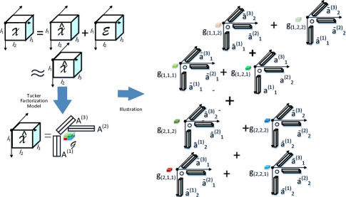
The main notations include the tensors, matrices and vectors, along with their basic elements and operations (in Table I). Fig. 1 illustrates the details of TD including the tanglement of the core tensor 𝒢𝒢\mathcal{G} with the N𝑁N factor matrices A(n)superscriptA𝑛\textbf{A}^{(n)}, n𝑛n \in {N}𝑁\{N\}. The data styles for TF include sparse and dense tensors and STD is devoted to HOHDST. Here, basic definitions for STD and models are rendered in Section 3.1. Finally, the STD process for the HOHDST is illustrated in Section 3.2.

TABLE I: Table of symbols.
Symbol Definition
Insubscript𝐼𝑛I_{n} The size of row in the n𝑛nth factor matrix;
Jnsubscript𝐽𝑛J_{n} The size of column in the n𝑛nth factor matrix;
𝒳𝒳\mathcal{X} Input N𝑁N order tensor \in +I1×I2××INsubscriptsuperscriptsubscript𝐼1subscript𝐼2subscript𝐼𝑁\mathbb{R}^{I_{1}\times I_{2}\times\cdots\times I_{N}}_{+};
xi1,i2,,insubscript𝑥subscript𝑖1subscript𝑖2subscript𝑖𝑛x_{i_{1},i_{2},\cdots,i_{n}} i1,i2,,insubscript𝑖1subscript𝑖2subscript𝑖𝑛i_{1},i_{2},\cdots,i_{n}th element of tensor 𝒳𝒳\mathcal{X};
𝒢𝒢\mathcal{G} Core N𝑁N order tensor \in J1×J2××JNsuperscriptsubscript𝐽1subscript𝐽2subscript𝐽𝑁\mathbb{R}^{J_{1}\times J_{2}\times\cdots\times J_{N}};
X Input matrix \in +I1×I2subscriptsuperscriptsubscript𝐼1subscript𝐼2\mathbb{R}^{I_{1}\times I_{2}}_{+};
X(n)superscriptX𝑛\textbf{X}^{(n)} n𝑛nth unfolding matrix for tensor 𝒳𝒳\mathcal{X};
Vecn(𝓧)\bm{\mathcal{X}}) n𝑛nth vectorization of a tensor 𝒳𝒳\mathcal{X};
ΩΩ\Omega Index (i1,,in,,iN)subscript𝑖1subscript𝑖𝑛subscript𝑖𝑁(i_{1},\cdots,i_{n},\cdots,i_{N}) of a tensor 𝒳𝒳\mathcal{X};
ΩM(n)subscriptsuperscriptΩ𝑛𝑀\Omega^{(n)}_{M} Index (in,j)subscript𝑖𝑛𝑗(i_{n},j) of n𝑛nth unfolding matrix X(n)superscriptX𝑛\textbf{X}^{(n)};
(ΩM(n))isubscriptsubscriptsuperscriptΩ𝑛𝑀𝑖(\Omega^{(n)}_{M})_{i} Column index set in i𝑖ith row of ΩM(n)subscriptsuperscriptΩ𝑛𝑀\Omega^{(n)}_{M};
(ΩM(n))jsuperscriptsubscriptsuperscriptΩ𝑛𝑀𝑗(\Omega^{(n)}_{M})^{j} Row index set in j𝑗jth column of ΩM(n)subscriptsuperscriptΩ𝑛𝑀\Omega^{(n)}_{M};
ΩV(n)subscriptsuperscriptΩ𝑛𝑉\Omega^{(n)}_{V} Index i𝑖i of n𝑛nth unfolding vector Vecn(𝓧𝓧\bm{\mathcal{X}});
{N}𝑁\{N\} The ordered set {1,2,,N1,N}12𝑁1𝑁\{1,2,\cdots,N-1,N\};
A(n)superscriptA𝑛\textbf{A}^{(n)} n𝑛nth feature matrix \in In×Jnsuperscriptsubscript𝐼𝑛subscript𝐽𝑛\mathbb{R}^{I_{n}\times J_{n}};
ain,:(n)superscriptsubscript𝑎subscript𝑖𝑛:𝑛a_{i_{n},:}^{(n)} insubscript𝑖𝑛i_{n}th row vector \in Knsuperscriptsubscript𝐾𝑛\mathbb{R}^{K_{n}} of A(n)superscriptA𝑛\textbf{A}^{(n)};
a:,j(n)superscriptsubscript𝑎:𝑗𝑛a_{:,j}^{(n)} j𝑗jth column vector \in Knsuperscriptsubscript𝐾𝑛\mathbb{R}^{K_{n}} of A(n)superscriptA𝑛\textbf{A}^{(n)};
ain,kn(n)superscriptsubscript𝑎subscript𝑖𝑛subscript𝑘𝑛𝑛a_{i_{n},k_{n}}^{(n)} knsubscript𝑘𝑛k_{n}th element of feature vector ain,:(n)superscriptsubscript𝑎subscript𝑖𝑛:𝑛a_{i_{n},:}^{(n)};
/(,/)\cdot\big{/}(-,/) Element-wise multiplication/\big{/} division;
\circ Outer production of vectors;
direct-product\odot Khatri-Rao (columnwise Kronecker) product;
×\times Matrix product;
×(n)subscript𝑛\times_{(n)} n𝑛n-Mode Tensor-Matrix product;
tensor-product\otimes Kronecker product.

3.1 Basic Definitions

Definition 1 (Tensor Unfolding (Matricization)).

n𝑛nth tensor unfolding (Matricization) refers to that a low order matrix X(n)In×I1In1In+1INsuperscriptX𝑛superscriptsubscript𝐼𝑛subscript𝐼1subscript𝐼𝑛1subscript𝐼𝑛1subscript𝐼𝑁\textbf{X}^{(n)}\in\mathbb{R}^{I_{n}\times I_{1}\cdots I_{n-1}\cdot I_{n+1}\cdot\cdots\cdot I_{N}} stores all information of a tensor 𝒳I1×I2×In×IN𝒳superscriptsubscript𝐼1subscript𝐼2subscript𝐼𝑛subscript𝐼𝑁\mathcal{X}\in\mathbb{R}^{I_{1}\times I_{2}\times\cdots I_{n}\cdots\times I_{N}} and the matrix element xin,j(n)subscriptsuperscript𝑥𝑛subscript𝑖𝑛𝑗x^{(n)}_{i_{n},j} of X(n)superscriptX𝑛\textbf{X}^{(n)} at the position j=1+k=1,nkN[(ik1)m=1,mnk1Im]𝑗1superscriptsubscriptformulae-sequence𝑘1𝑛𝑘𝑁delimited-[]subscript𝑖𝑘1superscriptsubscriptproductformulae-sequence𝑚1𝑚𝑛𝑘1subscript𝐼𝑚j=1+\sum_{k=1,n\neq k}^{N}\left[(i_{k}-1)\mathop{\prod}_{m=1,m\neq n}^{k-1}I_{m}\right] contains the tensor element xi1,i2,,insubscript𝑥subscript𝑖1subscript𝑖2subscript𝑖𝑛x_{i_{1},i_{2},\cdots,i_{n}} of a tensor 𝓧𝓧\bm{\mathcal{X}}.

Definition 2 (Vectorization of a tensor 𝓧𝓧\bm{\mathcal{X}}).

n𝑛nth tensor vectorization refers to that a vector x(n)superscript𝑥𝑛x^{(n)} (Vecn(𝓧𝓧\bm{\mathcal{X}}) and Vec(X(n)superscriptX𝑛\textbf{X}^{(n)})) stores all elements in the n𝑛nth matricization X(n)superscriptX𝑛\textbf{X}^{(n)} of a tensor 𝒳𝒳\mathcal{X} and xk(n)subscriptsuperscript𝑥𝑛𝑘x^{(n)}_{k} == Xi,j(n)subscriptsuperscriptX𝑛𝑖𝑗\textbf{X}^{(n)}_{i,j}, where k=(j1)In+i𝑘𝑗1subscript𝐼𝑛𝑖k=(j-1)I_{n}+i.

Definition 3 (Tensor Approximation).

A N𝑁N-order tensor 𝓧𝓧\bm{\mathcal{X}} \in I1××INsuperscriptsubscript𝐼1subscript𝐼𝑁\mathbb{R}^{I_{1}\times\cdots\times I_{N}} can be approximated by 𝓧^^𝓧\widehat{\bm{\mathcal{X}}} \in I1××INsuperscriptsubscript𝐼1subscript𝐼𝑁\mathbb{R}^{I_{1}\times\cdots\times I_{N}}, as well as a N𝑁N-order residual or noisy tensor 𝓔𝓔\bm{\mathcal{E}} \in I1××INsuperscriptsubscript𝐼1subscript𝐼𝑁\mathbb{R}^{I_{1}\times\cdots\times I_{N}}. The low-rank approximation problem is defined as 𝓧=𝓧^+𝓔𝓧^𝓧𝓔\bm{\mathcal{X}}=\widehat{\bm{\mathcal{X}}}+\bm{\mathcal{E}}, where 𝓧^^𝓧\widehat{\bm{\mathcal{X}}} is denoted by a low-rank tensor.

Refer to caption
Figure 1: Illustration of TD.
Definition 4 (n𝑛n-Mode Tensor-Matrix product).

n𝑛n-Mode Tensor-Matrix product is an operation which can reflect coordinate projection of a tensor 𝓧𝓧\bm{\mathcal{X}} \in I1××INsuperscriptsubscript𝐼1subscript𝐼𝑁\mathbb{R}^{I_{1}\times\cdots\times I_{N}} with projection matrix U \in In×Jnsuperscriptsubscript𝐼𝑛subscript𝐽𝑛\mathbb{R}^{I_{n}\times J_{n}} into a tensor (𝓧×(n)U)subscript𝑛𝓧U(\bm{\mathcal{X}}\times_{(n)}\textbf{U}) \in I1××In1×Jn×INsuperscriptsubscript𝐼1subscript𝐼𝑛1subscript𝐽𝑛subscript𝐼𝑁\mathbb{R}^{I_{1}\times\cdots\times I_{n-1}\times J_{n}\times\cdots I_{N}} where (𝓧×(n)U)i1××in1×jn×in+1××iNsubscriptsubscript𝑛𝓧Usubscript𝑖1subscript𝑖𝑛1subscript𝑗𝑛subscript𝑖𝑛1subscript𝑖𝑁(\bm{\mathcal{X}}\times_{(n)}\textbf{U})_{i_{1}\times\cdots\times i_{n-1}\times j_{n}\times i_{n+1}\times\cdots\times i_{N}} == in=1Insuperscriptsubscriptsubscript𝑖𝑛1subscript𝐼𝑛\sum\limits_{i_{n}=1}^{I_{n}} xi1××in××iNujn,insubscript𝑥subscript𝑖1subscript𝑖𝑛subscript𝑖𝑁subscript𝑢subscript𝑗𝑛subscript𝑖𝑛x_{i_{1}\times\cdots\times i_{n}\times\cdots\times i_{N}}u_{j_{n},i_{n}}.

Definition 5 (R𝑅R Kruskal Product).

For an N𝑁N-order tensor 𝓧^^𝓧\widehat{\bm{\mathcal{X}}} \in I1××INsuperscriptsubscript𝐼1subscript𝐼𝑁\mathbb{R}^{I_{1}\times\cdots\times I_{N}}, the R𝑅R Kruskal Product of 𝓧^^𝓧\widehat{\bm{\mathcal{X}}} is given by R𝑅R Kruskal product as: 𝓧^=r=1Ra:,r(1)a:,r(n)a:,r(N)^𝓧superscriptsubscript𝑟1𝑅subscriptsuperscript𝑎1:𝑟subscriptsuperscript𝑎𝑛:𝑟subscriptsuperscript𝑎𝑁:𝑟\widehat{\bm{\mathcal{X}}}=\sum_{r=1}^{R}a^{(1)}_{:,r}\circ\cdots\circ a^{(n)}_{:,r}\circ\cdots\circ a^{(N)}_{:,r}.

Definition 6 (Sparse Tucker Decomposition (STD)).

For a N𝑁N-order sparse tensor 𝓧𝓧\bm{\mathcal{X}} \in I1××INsuperscriptsubscript𝐼1subscript𝐼𝑁\mathbb{R}^{I_{1}\times\cdots\times I_{N}}, the STD of the optimal approximated 𝓧^^𝓧\widehat{\bm{\mathcal{X}}} is given by 𝓧^=𝒢×(1)A(1)×(2)×(n)A(n)×(n+1)×(N)A(N),^𝓧subscript𝑁subscript𝑛1subscript𝑛subscript2subscript1𝒢superscriptA1superscriptA𝑛superscriptA𝑁\widehat{\bm{\mathcal{X}}}=\mathcal{G}\times_{(1)}\textbf{A}^{(1)}\times_{(2)}\cdots\times_{(n)}\textbf{A}^{(n)}\times_{(n+1)}\cdots\times_{(N)}\textbf{A}^{(N)}, where 𝒢𝒢\mathcal{G} is the core tensor and A(n)superscriptA𝑛\textbf{A}^{(n)}, n{N}𝑛𝑁n\in\{N\} are the low-rank factor matrices. The rank of TF for a tensor is [J1,,Jn,,JN]subscript𝐽1subscript𝐽𝑛subscript𝐽𝑁[J_{1},\cdots,J_{n},\cdots,J_{N}]. The determination process for the core tensor 𝒢𝒢\mathcal{G} and factor matrices A(n)superscriptA𝑛\textbf{A}^{(n)}, n{N}𝑛𝑁n\in\{N\} follows the sparsity model of the sparse tensor 𝓧𝓧\bm{\mathcal{X}}.

In the convex optimization community, the literature [49] gives the definition of Lipschitz-continuity with constant L𝐿L and strong convexity with constant μ𝜇\mu.

Definition 7 (L𝐿L-Lipschitz continuity).

A continuously differentiable function f(x)𝑓xf(\textbf{x}) is called L𝐿L-smooth on rsuperscript𝑟\mathbb{R}^{r} if the gradient f(x)𝑓x\nabla f(\textbf{x}) is L𝐿L-Lipschitz continuous for any x, y \in rsuperscript𝑟\mathbb{R}^{r}, that is \| f(x)𝑓x\nabla f(\textbf{x}) - f(y)𝑓y\nabla f(\textbf{y}) 2\|_{2} \leq L𝐿L \| x - y 2\|_{2}, where 2\|\bullet\|_{2} is L2subscript𝐿2L_{2}-norm x2subscriptnormx2\|\textbf{x}\|_{2} == (k=1rxk2)1/2superscriptsuperscriptsubscript𝑘1𝑟superscriptsubscript𝑥𝑘212(\mathbb{\sum}_{k=1}^{r}x_{k}^{2})^{1/2} for a vector x.

Definition 8 (μ𝜇\mu-Convex).

A continuously differentiable function f(x)𝑓xf(\textbf{x}) is called strongly-convex on rsuperscript𝑟\mathbb{R}^{r} if there exists a constant μ𝜇\mu >> 00 for any x, y \in rsuperscript𝑟\mathbb{R}^{r}, that is f(x)𝑓xf(\textbf{x}) \geq f(y)𝑓yf(\textbf{y}) ++ \nabla f(y)𝑓yf(\textbf{y}) (xy)Tsuperscriptxy𝑇(\textbf{x}-\textbf{y})^{T} ++ 12μxy2212𝜇superscriptsubscriptnormxy22\frac{1}{2}\mu\|\textbf{x}-\textbf{y}\|_{2}^{2}.

Due to limited spaces, we provide the description of basic optimization as the supplementary material.

3.2 Problems for Large-scale Optimization Problems

Many ML tasks are transformed into the solvent of optimization problem [32, 35, 33, 34] and the basis optimization problem is organized as:

argminwRf(w)subscript𝑤superscript𝑅𝑓𝑤\displaystyle\mathop{\arg\min}_{w\in\mathbb{R}^{R}}f(w) =L(w|yi,xi,w)LossFunction+λwR(w)RegularizationItemabsentsubscript𝐿conditional𝑤subscript𝑦𝑖subscript𝑥𝑖𝑤𝐿𝑜𝑠𝑠𝐹𝑢𝑛𝑐𝑡𝑖𝑜𝑛subscriptsubscript𝜆𝑤𝑅𝑤𝑅𝑒𝑔𝑢𝑙𝑎𝑟𝑖𝑧𝑎𝑡𝑖𝑜𝑛𝐼𝑡𝑒𝑚\displaystyle=\underbrace{L\bigg{(}w\bigg{|}y_{i},x_{i},w\bigg{)}}_{Loss\ Function}+\underbrace{\lambda_{w}R(w)}_{Regularization\ Item} (1)
=i=1NLi(w|yi,xi,w)+λwRi(w),absentsuperscriptsubscript𝑖1𝑁subscript𝐿𝑖conditional𝑤subscript𝑦𝑖subscript𝑥𝑖𝑤subscript𝜆𝑤subscript𝑅𝑖𝑤\displaystyle=\sum\limits_{i=1}^{N}L_{i}\bigg{(}w\bigg{|}y_{i},x_{i},w\bigg{)}+\lambda_{w}R_{i}(w),

where yisubscript𝑦𝑖y_{i} \in 1superscript1\mathbb{R}^{1}, xisubscript𝑥𝑖x_{i} \in Rsuperscript𝑅\mathbb{R}^{R}, i{N}𝑖𝑁i\in\{N\}, wR𝑤superscript𝑅w\in\mathbb{R}^{R} and the original optimization model needs gradient which should select all the samples {xi|i{N}}conditional-setsubscript𝑥𝑖𝑖𝑁\{x_{i}|i\in\{N\}\} from the dataset ΩΩ\Omega and the GD is presented as:

w𝑤\displaystyle w wγfΩ(w)wabsent𝑤𝛾subscript𝑓Ω𝑤𝑤\displaystyle\leftarrow w-\gamma\frac{\partial f_{\Omega}(w)}{\partial w} (2)
=wγ1Ni=1N(Li(w)+λwRi(w))w.absent𝑤𝛾1𝑁superscriptsubscript𝑖1𝑁subscript𝐿𝑖𝑤subscript𝜆𝑤subscript𝑅𝑖𝑤𝑤\displaystyle=w-\gamma\frac{1}{N}\sum\limits_{i=1}^{N}\frac{\partial\bigg{(}L_{i}(w)+\lambda_{w}R_{i}(w)\bigg{)}}{\partial w}.

The second-order solution, i.e., ALS and CD, etc, are deduced from the construction of GD from the whole dataset. In large-scale optimization scenarios, SGD is a common strategy [32, 35, 33, 34] and promises to obtain the optimal accuracy via a certain number of training epoches [32, 35, 33, 34]. An M𝑀M entries set ΨΨ\Psi is randomly selected from the set ΩΩ\Omega, and the SGD is presented as:

w𝑤\displaystyle w wγfΨ(w)wabsent𝑤𝛾subscript𝑓Ψ𝑤𝑤\displaystyle\leftarrow w-\gamma\frac{\partial f_{\Psi}(w)}{\partial w} (3)
wγ1MiΨ(Li(w)+λwRi(w))w.absent𝑤𝛾1𝑀subscript𝑖Ψsubscript𝐿𝑖𝑤subscript𝜆𝑤subscript𝑅𝑖𝑤𝑤\displaystyle\approx w-\gamma\frac{1}{M}\sum\limits_{i\in\Psi}\frac{\partial\bigg{(}L_{i}(w)+\lambda_{w}R_{i}(w)\bigg{)}}{\partial w}.

Equ. (3) is an average SGD [33], and the averaged SG can be applied to build the basic tool of the modern stochastic optimization strategies, e.g., Stochastic Recursive Gradient [34], variance SGD [32], or momentum SGD [35], which can retain robustness and fast convergence. The optimization function can be packaged in the form of SGD(M,λ,γ,w,fΨ(w)w)𝑆𝐺𝐷𝑀𝜆𝛾𝑤subscript𝑓Ψ𝑤𝑤SGD\bigg{(}M,\lambda,\gamma,w,\frac{\partial f_{\Psi}(w)}{\partial w}\bigg{)}.

Refer to caption
Figure 2: Illustration of Optimization Process for SGD__\_Tucker: 1) Original problem for core tensor, 2) Kruskal product for approximating core tensor, 3) Optimization process for factor matrices.

4 SGD__\_Tucker

Overview: In this section, SGD__\_Tucker is proposed to decompose the optimization objectives which involves frequent operations of intermediate matrices into a problem which only needs the manipulations of small batches of intermediate matrices. Fig. 2 illustrates the framework for our work. As Fig. 2 shows, SGD__\_Tucker comprises of an approximation process of the core tensor and an optimization for factor matrices. Table II records the intermediate variables which follow the problem deduction process. Section 4.1 presents the deduction process for the core tensor (Lines 1-16, Algorithm 1), and Section 4.2 presents the proceeding process for the factor matrices of SGD__\_Tucker (Lines 17-26, Algorithm 1). Section 4.3 shows the stochastic optimization process for the proposed novel optimization objectives, which illustrates the details of the process that how can the SGD__\_Tucker divide the high-dimension intermediate matrices {H(n),S(n),E(n)|n{N}}conditional-setsuperscriptH𝑛superscriptS𝑛superscriptE𝑛𝑛𝑁\bigg{\{}\textbf{H}^{(n)},\textbf{S}^{(n)},\textbf{E}^{(n)}\big{|}n\in\{N\}\bigg{\}} into a small batches of intermediate matrices. Section 4.4 shows the parallel and distributed strategies for SGD__\_Tucker. Finally, section 4.5 illustrates the analysis of space and time complexities. Because the optimization process for approximating the core tensor and factor matrices are non-convex. We fix the core tensor and optimize a factor matrix and fix factor matrices to optimize Kruskal product for core tensor. This alternative minimization strategy is a convex solution [46, 47, 48, 50].

TABLE II: Table of Intermediate Varibles for SGD__\_Tucker.
Symbol Description Emerging
Equations
𝓖^^𝓖\widehat{\bm{\mathcal{G}}} \in +J1×J2××JNsubscriptsuperscriptsubscript𝐽1subscript𝐽2subscript𝐽𝑁\mathbb{R}^{J_{1}\times J_{2}\times\cdots\times J_{N}}_{+} coresubscript𝑐𝑜𝑟𝑒\mathbb{R}_{core} Kruskal Equ. (4);
product for 𝓖𝓖\bm{\mathcal{G}}
B(n)Jn×RcoresuperscriptB𝑛superscriptsubscript𝐽𝑛subscript𝑅𝑐𝑜𝑟𝑒\textbf{B}^{(n)}\in\mathbb{R}^{J_{n}\times R_{core}} n𝑛nth Kruskal matrix for 𝓖^^𝓖\widehat{\bm{\mathcal{G}}} Equ. (4);
g^(n)superscript^𝑔𝑛\widehat{g}^{(n)} \in n=1NJnsuperscriptsuperscriptsubscriptproduct𝑛1𝑁subscript𝐽𝑛\mathbb{R}^{\prod\limits_{n=1}^{N}J_{n}} n𝑛nth vectorization Equ. (5);
of tensor 𝓖^^𝓖\widehat{\bm{\mathcal{G}}}
H(n)superscriptH𝑛\textbf{H}^{(n)} \in n=1NIn×n=1NJnsuperscriptsuperscriptsubscriptproduct𝑛1𝑁subscript𝐼𝑛superscriptsubscriptproduct𝑛1𝑁subscript𝐽𝑛\mathbb{R}^{\prod\limits_{n=1}^{N}I_{n}\times\prod\limits_{n=1}^{N}J_{n}} Coefficient for g^(n)superscript^𝑔𝑛\widehat{g}^{(n)} Equ. (5);
x(n)superscript𝑥𝑛x^{(n)} \in n=1NInsuperscriptsuperscriptsubscriptproduct𝑛1𝑁subscript𝐼𝑛\mathbb{R}^{\prod\limits_{n=1}^{N}I_{n}} n𝑛nth vectorization of Equ. (5);
Tensor 𝒳𝒳\mathcal{X}
Q(n)superscriptQ𝑛\textbf{Q}^{(n)} \in r=1,rnNJr×Rcoresuperscriptsuperscriptsubscriptproductformulae-sequence𝑟1𝑟𝑛𝑁subscript𝐽𝑟subscript𝑅𝑐𝑜𝑟𝑒\mathbb{R}^{\prod\limits_{r=1,r\neq n}^{N}J_{r}\times R_{core}} Coefficient of B(n)superscriptB𝑛\textbf{B}^{(n)} Equ. (6);
for constructing g^(n)superscript^𝑔𝑛\widehat{g}^{(n)}
U(n)superscriptU𝑛\textbf{U}^{(n)} \in Jn×Jnsuperscriptsubscript𝐽𝑛subscript𝐽𝑛\mathbb{R}^{J_{n}\times J_{n}} Unity matrix Equ. (7);
Or(n)subscriptsuperscriptO𝑛𝑟\textbf{O}^{(n)}_{r} \in r=1NJr×Jnsuperscriptsuperscriptsubscriptproduct𝑟1𝑁subscript𝐽𝑟subscript𝐽𝑛\mathbb{R}^{\prod\limits_{r=1}^{N}J_{r}\times J_{n}} Coefficient of b:,r(n)subscriptsuperscript𝑏𝑛:𝑟b^{(n)}_{:,r} Equ. (8);
for constructing g^(n)superscript^𝑔𝑛\widehat{g}^{(n)}
xrcore(n)subscriptsuperscript𝑥𝑛subscript𝑟𝑐𝑜𝑟𝑒x^{(n)}_{r_{core}} \in r=1NIrsuperscriptsuperscriptsubscriptproduct𝑟1𝑁subscript𝐼𝑟\mathbb{R}^{\prod\limits_{r=1}^{N}I_{r}} Intermediate vector of x(n)superscript𝑥𝑛x^{(n)} Equ. (9);
Hrcore(n)subscriptsuperscriptH𝑛subscript𝑟𝑐𝑜𝑟𝑒\textbf{H}^{(n)}_{r_{core}} \in n=1NIn×Jnsuperscriptsuperscriptsubscriptproduct𝑛1𝑁subscript𝐼𝑛subscript𝐽𝑛\mathbb{R}^{\prod\limits_{n=1}^{N}I_{n}\times J_{n}} Coefficient of b:,r(n)subscriptsuperscript𝑏𝑛:𝑟b^{(n)}_{:,r} Equ. (9);
for constructing g^(n)superscript^𝑔𝑛\widehat{g}^{(n)}
S(n)superscriptS𝑛\textbf{S}^{(n)} \in k=1,knNJn×k=1,knNIksuperscriptsuperscriptsubscriptproductformulae-sequence𝑘1𝑘𝑛𝑁subscript𝐽𝑛superscriptsubscriptproductformulae-sequence𝑘1𝑘𝑛𝑁subscript𝐼𝑘\mathbb{R}^{\prod\limits_{k=1,k\neq n}^{N}J_{n}\times\prod\limits_{k=1,k\neq n}^{N}I_{k}} Coefficient of A(n)G^(n)superscriptA𝑛superscript^G𝑛\textbf{A}^{(n)}\widehat{\textbf{G}}^{(n)} Equ. (10);
for constructing 𝑿^(n)superscript^𝑿𝑛\widehat{\bm{X}}^{(n)}
E(n)superscriptE𝑛\textbf{E}^{(n)} \in Jn×k=1,knNIksuperscriptsubscript𝐽𝑛superscriptsubscriptproductformulae-sequence𝑘1𝑘𝑛𝑁subscript𝐼𝑘\mathbb{R}^{J_{n}\times\prod\limits_{k=1,k\neq n}^{N}I_{k}} Coefficient of A(n)superscriptA𝑛\textbf{A}^{(n)} Equ. (11);
for constructing 𝑿^(n)superscript^𝑿𝑛\widehat{\bm{X}}^{(n)}
xΨV(n)(n)subscriptsuperscript𝑥𝑛subscriptsuperscriptΨ𝑛𝑉x^{(n)}_{\Psi^{(n)}_{V}} \in |ΨV(n)|superscriptsubscriptsuperscriptΨ𝑛𝑉\mathbb{R}^{|\Psi^{(n)}_{V}|} Partial vector x(n)superscript𝑥𝑛x^{(n)} from set ΨΨ\Psi Equ. (14);
HΨV(n),:(n)superscriptsubscriptHsubscriptsuperscriptΨ𝑛𝑉:𝑛\textbf{H}_{\Psi^{(n)}_{V},:}^{(n)} \in |ΨV(n)|×n=1NJnsuperscriptsubscriptsuperscriptΨ𝑛𝑉superscriptsubscriptproduct𝑛1𝑁subscript𝐽𝑛\mathbb{R}^{|\Psi^{(n)}_{V}|\times\prod\limits_{n=1}^{N}J_{n}} Partial matrix of H(n)superscriptH𝑛\textbf{H}^{(n)} Equ. (14);
𝑿:,(ΨM(n))in(n)superscriptsubscript𝑿:subscriptsubscriptsuperscriptΨ𝑛𝑀subscript𝑖𝑛𝑛\bm{X}_{:,(\Psi^{(n)}_{M})_{i_{n}}}^{(n)} \in In×|(ΨM(n))in|superscriptsubscript𝐼𝑛subscriptsubscriptsuperscriptΨ𝑛𝑀subscript𝑖𝑛\mathbb{R}^{I_{n}\times|(\Psi^{(n)}_{M})_{i_{n}}|} Partial matrix of 𝑿(n)superscript𝑿𝑛\bm{X}^{(n)} Equ. (17);
E:,(ΨM(n))in(n)subscriptsuperscriptE𝑛:subscriptsubscriptsuperscriptΨ𝑛𝑀subscript𝑖𝑛\textbf{E}^{(n)}_{:,(\Psi^{(n)}_{M})_{i_{n}}} \in Jn×|(ΨM(n))in|superscriptsubscript𝐽𝑛subscriptsubscriptsuperscriptΨ𝑛𝑀subscript𝑖𝑛\mathbb{R}^{J_{n}\times|(\Psi^{(n)}_{M})_{i_{n}}|} Partial matrix of E(n)superscriptE𝑛\textbf{E}^{(n)} Equ. (17).

4.1 Optimization Process for the Core Tensor

Due to the non-trivial coupling of the core tensor 𝓖𝓖\bm{\mathcal{G}}, the efficient and effective way to infer it is through an approximation. A tensor 𝓖𝓖\bm{\mathcal{G}} can be approximated by Rcoresubscript𝑅𝑐𝑜𝑟𝑒R_{core} \leq Jn,n{N}subscript𝐽𝑛𝑛𝑁{J_{n},n\in\{N\}} Kruskal product of low-rank matrices {B(n)Jn×Rcore|n{N}}conditional-setsuperscriptB𝑛superscriptsubscript𝐽𝑛subscript𝑅𝑐𝑜𝑟𝑒𝑛𝑁\{\textbf{B}^{(n)}\in\mathbb{R}^{J_{n}\times R_{core}}|n\in\{N\}\} to form 𝓖^^𝓖\widehat{\bm{\mathcal{G}}}:

𝓖^=rcore=1Rcoreb:,rcore(1)b:,rcore(n)b:,rcore(N).^𝓖superscriptsubscriptsubscript𝑟𝑐𝑜𝑟𝑒1subscript𝑅𝑐𝑜𝑟𝑒subscriptsuperscript𝑏1:subscript𝑟𝑐𝑜𝑟𝑒subscriptsuperscript𝑏𝑛:subscript𝑟𝑐𝑜𝑟𝑒subscriptsuperscript𝑏𝑁:subscript𝑟𝑐𝑜𝑟𝑒\displaystyle\widehat{\bm{\mathcal{G}}}=\sum_{r_{core}=1}^{R_{core}}b^{(1)}_{:,r_{core}}\circ\cdots\circ b^{(n)}_{:,r_{core}}\circ\cdots\circ b^{(N)}_{:,r_{core}}. (4)

As the direct approximation for the core tensor 𝓖𝓖\bm{\mathcal{G}} may result in instability, we propose to apply the coupling process to approximate STD and tensor approximation. Specifically, we use Kruskal product of low-rank matrices{B(n)Jn×Rcore|n{N}}conditional-setsuperscriptB𝑛superscriptsubscript𝐽𝑛subscript𝑅𝑐𝑜𝑟𝑒𝑛𝑁\{\textbf{B}^{(n)}\in\mathbb{R}^{J_{n}\times R_{core}}|n\in\{N\}\} as follows:

argmin𝓖^fsubscript^𝓖𝑓\displaystyle\mathop{\arg\min}_{\widehat{\bm{\mathcal{G}}}}f (g^(n)|x(n),{A(n)})conditionalsuperscript^𝑔𝑛superscript𝑥𝑛superscriptA𝑛\displaystyle\bigg{(}\widehat{g}^{(n)}\bigg{|}x^{(n)},\{\textbf{A}^{(n)}\}\bigg{)} (5)
=\displaystyle= x(n)H(n)g^(n)22+λg^(n)g^(n)22,superscriptsubscriptnormsuperscript𝑥𝑛superscriptH𝑛superscript^𝑔𝑛22subscript𝜆superscript^𝑔𝑛superscriptsubscriptnormsuperscript^𝑔𝑛22\displaystyle\bigg{\|}x^{(n)}-\textbf{H}^{(n)}\widehat{g}^{(n)}\bigg{\|}_{2}^{2}+\lambda_{\widehat{g}^{(n)}}\bigg{\|}\widehat{g}^{(n)}\bigg{\|}_{2}^{2},

where g^(n)superscript^𝑔𝑛\widehat{g}^{(n)} == Vec(B(n)Q(n)T)𝑉𝑒𝑐superscriptB𝑛superscriptQsuperscript𝑛𝑇Vec(\textbf{B}^{(n)}\textbf{Q}^{(n)^{T}}) and Q(n)superscriptQ𝑛\textbf{Q}^{(n)} == B(N)B(n+1)B(n1)B(1)direct-productsuperscriptB𝑁superscriptB𝑛1superscriptB𝑛1superscriptB1\textbf{B}^{(N)}\odot\cdots\odot\textbf{B}^{(n+1)}\odot\textbf{B}^{(n-1)}\odot\cdots\odot\textbf{B}^{(1)}. The tanglement problem resulted from Rcoresubscript𝑅𝑐𝑜𝑟𝑒R_{core} Kruskal product of low-rank matrices {B(n)Jn×Rcore|n{N}}conditional-setsuperscriptB𝑛superscriptsubscript𝐽𝑛subscript𝑅𝑐𝑜𝑟𝑒𝑛𝑁\{\textbf{B}^{(n)}\in\mathbb{R}^{J_{n}\times R_{core}}|n\in\{N\}\} leads to a non-convex optimization problem for the optimization objective (5). The alternative optimization strategy [50] is adopted to update the parameters {B(n)Jn×Rcore|n{N}}conditional-setsuperscriptB𝑛superscriptsubscript𝐽𝑛subscript𝑅𝑐𝑜𝑟𝑒𝑛𝑁\{\textbf{B}^{(n)}\in\mathbb{R}^{J_{n}\times R_{core}}|n\in\{N\}\} and then the non-convex optimization objective (5) is turned into the objective as:

argminB(n),n{N}subscriptsuperscriptB𝑛𝑛𝑁\displaystyle\mathop{\arg\min}_{\textbf{B}^{(n)},n\in\{N\}} f(B(n)|x(n),{A(n)},{B(n)})𝑓conditionalsuperscriptB𝑛superscript𝑥𝑛superscriptA𝑛superscriptB𝑛\displaystyle f\bigg{(}\textbf{B}^{(n)}\bigg{|}x^{(n)},\{\textbf{A}^{(n)}\},\{\textbf{B}^{(n)}\}\bigg{)} (6)
=\displaystyle= x(n)H(n)Vec(B(n)Q(n)T)22+λBB22,superscriptsubscriptnormsuperscript𝑥𝑛superscriptH𝑛𝑉𝑒𝑐superscriptB𝑛superscriptQsuperscript𝑛𝑇22subscript𝜆BsuperscriptsubscriptnormB22\displaystyle\bigg{\|}x^{(n)}-\textbf{H}^{(n)}Vec(\textbf{B}^{(n)}\textbf{Q}^{(n)^{T}})\bigg{\|}_{2}^{2}+\lambda_{\textbf{B}}\bigg{\|}\textbf{B}\bigg{\|}_{2}^{2},

where Vec(B(n)Q(n)T)𝑉𝑒𝑐superscriptB𝑛superscriptQsuperscript𝑛𝑇Vec(\textbf{B}^{(n)}\textbf{Q}^{(n)^{T}}) == Vec(r=1Rcoreb:,r(n)q:,r(n)T)𝑉𝑒𝑐superscriptsubscript𝑟1subscript𝑅𝑐𝑜𝑟𝑒subscriptsuperscript𝑏𝑛:𝑟superscriptsubscript𝑞:𝑟superscript𝑛𝑇Vec(\sum\limits_{r=1}^{R_{core}}b^{(n)}_{:,r}q_{:,r}^{(n)^{T}}).

The optimization objective (6) is not explicit for the variable B(n),n{N}superscriptB𝑛𝑛𝑁\textbf{B}^{(n)},n\in\{N\} and it is hard to find the gradient of the variables B(n),n{N}superscriptB𝑛𝑛𝑁\textbf{B}^{(n)},n\in\{N\} under the current formulation. Thus, we borrow the intermediate variables with a unity matrix as Or(n)subscriptsuperscriptO𝑛𝑟\textbf{O}^{(n)}_{r} \in k=1NJk×Jnsuperscriptsuperscriptsubscriptproduct𝑘1𝑁subscript𝐽𝑘subscript𝐽𝑛\mathbb{R}^{\prod_{k=1}^{N}J_{k}\times J_{n}}, r𝑟r \in {Rcore}subscript𝑅𝑐𝑜𝑟𝑒\{R_{core}\} and the unity matrix U(n)superscriptU𝑛\textbf{U}^{(n)} \in Jn×Jnsuperscriptsubscript𝐽𝑛subscript𝐽𝑛\mathbb{R}^{J_{n}\times J_{n}}, n{N}𝑛𝑁n\in\{N\} which can present the variables B(n),n{N}superscriptB𝑛𝑛𝑁\textbf{B}^{(n)},n\in\{N\} in a gradient-explicit formation. The matrix Or(n)subscriptsuperscriptO𝑛𝑟\textbf{O}^{(n)}_{r} is defined as

Or(n)=[\displaystyle\textbf{O}^{(n)}_{r}=\bigg{[} q1,rU(n),,qm,rU(n),,subscript𝑞1𝑟superscriptU𝑛subscript𝑞𝑚𝑟superscriptU𝑛\displaystyle q_{1,r}\textbf{U}^{(n)},\cdots,q_{m,r}\textbf{U}^{(n)},\cdots, (7)
qk=1,knNJk,rU(n)]T.\displaystyle q_{\prod\limits_{k=1,k\neq n}^{N}J_{k},r}\textbf{U}^{(n)}\bigg{]}^{T}.

The key transformation of the gradient-explicit formation for the variables B(n),n{N}superscriptB𝑛𝑛𝑁\textbf{B}^{(n)},n\in\{N\} is as Vec(r=1Rcoreb:,r(n)q:,r(n)T)=r=1RcoreOr(n)b:,r(n)𝑉𝑒𝑐superscriptsubscript𝑟1subscript𝑅𝑐𝑜𝑟𝑒subscriptsuperscript𝑏𝑛:𝑟superscriptsubscript𝑞:𝑟superscript𝑛𝑇superscriptsubscript𝑟1subscript𝑅𝑐𝑜𝑟𝑒subscriptsuperscriptO𝑛𝑟subscriptsuperscript𝑏𝑛:𝑟Vec(\sum\limits_{r=1}^{R_{core}}b^{(n)}_{:,r}q_{:,r}^{(n)^{T}})=\sum\limits_{r=1}^{R_{core}}\textbf{O}^{(n)}_{r}b^{(n)}_{:,r}. Then the optimization objective (6) is reformulated into:

argminB(n),n{N}subscriptsuperscriptB𝑛𝑛𝑁\displaystyle\mathop{\arg\min}_{\textbf{B}^{(n)},n\in\{N\}} f(B(n)|x(n),{A(n)},{B(n)})𝑓conditionalsuperscriptB𝑛superscript𝑥𝑛superscriptA𝑛superscriptB𝑛\displaystyle f\bigg{(}\textbf{B}^{(n)}\bigg{|}x^{(n)},\{\textbf{A}^{(n)}\},\{\textbf{B}^{(n)}\}\bigg{)} (8)
=x(n)H(n)r=1RcoreOr(n)b:,r(n)22+λBB22.absentsuperscriptsubscriptnormsuperscript𝑥𝑛superscriptH𝑛superscriptsubscript𝑟1subscript𝑅𝑐𝑜𝑟𝑒subscriptsuperscriptO𝑛𝑟subscriptsuperscript𝑏𝑛:𝑟22subscript𝜆BsuperscriptsubscriptnormB22\displaystyle=\bigg{\|}x^{(n)}-\textbf{H}^{(n)}\sum\limits_{r=1}^{R_{core}}\textbf{O}^{(n)}_{r}b^{(n)}_{:,r}\bigg{\|}_{2}^{2}+\lambda_{\textbf{B}}\bigg{\|}\textbf{B}\bigg{\|}_{2}^{2}.

The cyclic block optimization strategy [51] is adopted to update the variables {b:,rcore(n)|rcore{Rcore}}conditional-setsubscriptsuperscript𝑏𝑛:subscript𝑟𝑐𝑜𝑟𝑒subscript𝑟𝑐𝑜𝑟𝑒subscript𝑅𝑐𝑜𝑟𝑒\big{\{}b^{(n)}_{:,r_{core}}|r_{core}\in\{R_{core}\}\big{\}} within a low-rank matrix B(n),n{N}superscriptB𝑛𝑛𝑁\textbf{B}^{(n)},n\in\{N\} and eventually the optimization objective is reformulated into:

argminb:,rcore(n),n{N}subscriptsubscriptsuperscript𝑏𝑛:subscript𝑟𝑐𝑜𝑟𝑒𝑛𝑁\displaystyle\mathop{\arg\min}_{b^{(n)}_{:,r_{core}},n\in\{N\}} f(b:,rcore(n)|x(n),{A(n)},{B(n)})𝑓conditionalsubscriptsuperscript𝑏𝑛:subscript𝑟𝑐𝑜𝑟𝑒superscript𝑥𝑛superscriptA𝑛superscriptB𝑛\displaystyle f\bigg{(}b^{(n)}_{:,r_{core}}\bigg{|}x^{(n)},\{\textbf{A}^{(n)}\},\{\textbf{B}^{(n)}\}\bigg{)} (9)
=\displaystyle= xrcore(n)Hrcore(n)b:,rcore(n)22+λBb:,rcore(n)22,superscriptsubscriptnormsubscriptsuperscript𝑥𝑛subscript𝑟𝑐𝑜𝑟𝑒subscriptsuperscriptH𝑛subscript𝑟𝑐𝑜𝑟𝑒subscriptsuperscript𝑏𝑛:subscript𝑟𝑐𝑜𝑟𝑒22subscript𝜆Bsuperscriptsubscriptnormsubscriptsuperscript𝑏𝑛:subscript𝑟𝑐𝑜𝑟𝑒22\displaystyle\bigg{\|}x^{(n)}_{r_{core}}-\textbf{H}^{(n)}_{r_{core}}b^{(n)}_{:,r_{core}}\bigg{\|}_{2}^{2}+\lambda_{\textbf{B}}\bigg{\|}b^{(n)}_{:,r_{core}}\bigg{\|}_{2}^{2},

where xrcore(n)subscriptsuperscript𝑥𝑛subscript𝑟𝑐𝑜𝑟𝑒x^{(n)}_{r_{core}} == x(n)H(n)r=1,rrcoreRcoreOr(n)b:,r(n)superscript𝑥𝑛superscriptH𝑛superscriptsubscriptformulae-sequence𝑟1𝑟subscript𝑟𝑐𝑜𝑟𝑒subscript𝑅𝑐𝑜𝑟𝑒subscriptsuperscriptO𝑛𝑟subscriptsuperscript𝑏𝑛:𝑟x^{(n)}-\textbf{H}^{(n)}\sum\limits_{r=1,r\neq r_{core}}^{R_{core}}\textbf{O}^{(n)}_{r}b^{(n)}_{:,r} and Hrcore(n)subscriptsuperscriptH𝑛subscript𝑟𝑐𝑜𝑟𝑒\textbf{H}^{(n)}_{r_{core}} == H(n)Orcore(n)n=1NIn×JnsuperscriptH𝑛subscriptsuperscriptO𝑛subscript𝑟𝑐𝑜𝑟𝑒superscriptsuperscriptsubscriptproduct𝑛1𝑁subscript𝐼𝑛subscript𝐽𝑛\textbf{H}^{(n)}\textbf{O}^{(n)}_{r_{core}}\in\mathbb{R}^{\prod\limits_{n=1}^{N}I_{n}\times J_{n}}.

Theorem 1.

From the function form of (9), the optimization objective for b:,rcore(n)subscriptsuperscript𝑏𝑛:subscript𝑟𝑐𝑜𝑟𝑒b^{(n)}_{:,r_{core}} is a u𝑢u-convex and L𝐿L-smooth function.

Proof.

The proof is divided into the following two parts: 1) The non-convex optimization problem is transformed into fixing factor matrices A(n),n{N}superscriptA𝑛𝑛𝑁\textbf{A}^{(n)},n\in\{N\} and updating core tensor part, and this transformation can keep promise that convex optimization for each part and appropriate accuracy [46, 47, 48, 50]. 2) The distance function xrcore(n)Hrcore(n)b:,rcore(n)22superscriptsubscriptnormsubscriptsuperscript𝑥𝑛subscript𝑟𝑐𝑜𝑟𝑒subscriptsuperscriptH𝑛subscript𝑟𝑐𝑜𝑟𝑒subscriptsuperscript𝑏𝑛:subscript𝑟𝑐𝑜𝑟𝑒22\big{\|}x^{(n)}_{r_{core}}-\textbf{H}^{(n)}_{r_{core}}b^{(n)}_{:,r_{core}}\big{\|}_{2}^{2} is an Euclidean distance with L2subscript𝐿2L_{2} norm regularization λBb:,rcore(n)22subscript𝜆Bsuperscriptsubscriptnormsubscriptsuperscript𝑏𝑛:subscript𝑟𝑐𝑜𝑟𝑒22\lambda_{\textbf{B}}\big{\|}b^{(n)}_{:,r_{core}}\big{\|}_{2}^{2} [52]. Thus, the optimization objective (9) is a u𝑢u-convex and L𝐿L-smooth function obviously [50], [53], [49]. The proof details are omitted which can be found on [32], [54]. ∎

4.2 Optimization Process for Factor Matrices

After the optimization step is conducted for {B(n)Jn×Rcore|n{N}}conditional-setsuperscriptB𝑛superscriptsubscript𝐽𝑛subscript𝑅𝑐𝑜𝑟𝑒𝑛𝑁\{\textbf{B}^{(n)}\in\mathbb{R}^{J_{n}\times R_{core}}|n\in\{N\}\}, the Kruskal product for approximated core tensor g^(n)superscript^𝑔𝑛\hat{g}^{(n)} is constructed by Equ. (4). Thus, we should consider the optimization problem for factor matrices A(n),{n|n{N}}superscriptA𝑛conditional-set𝑛𝑛𝑁\textbf{A}^{(n)},\{n|n\in\{N\}\} as:

argminA(n),n{N}subscriptsuperscriptA𝑛𝑛𝑁\displaystyle\mathop{\arg\min}_{\textbf{A}^{(n)},n\in\{N\}} f(A(n)|𝑿(n),{A(n)},G^(n))𝑓conditionalsuperscriptA𝑛superscript𝑿𝑛superscriptA𝑛superscript^G𝑛\displaystyle f\bigg{(}\textbf{A}^{(n)}\bigg{|}\bm{X}^{(n)},\big{\{}\textbf{A}^{(n)}\big{\}},\widehat{\textbf{G}}^{(n)}\bigg{)} (10)
=𝑿(n)𝑿^(n)22+λAA(n)22,absentsuperscriptsubscriptnormsuperscript𝑿𝑛superscript^𝑿𝑛22subscript𝜆AsuperscriptsubscriptnormsuperscriptA𝑛22\displaystyle=\bigg{\|}\bm{X}^{(n)}-\widehat{\bm{X}}^{(n)}\bigg{\|}_{2}^{2}+\lambda_{\textbf{A}}\bigg{\|}\textbf{A}^{(n)}\bigg{\|}_{2}^{2},

where 𝑿^(n)superscript^𝑿𝑛\widehat{\bm{X}}^{(n)} == A(n)G^(n)S(n)TsuperscriptA𝑛superscript^G𝑛superscriptSsuperscript𝑛𝑇\textbf{A}^{(n)}\widehat{\textbf{G}}^{(n)}\textbf{S}^{(n)^{T}} and S(n)superscriptS𝑛\textbf{S}^{(n)} == A(N)A(n+1)A(n1)A(1)tensor-productsuperscriptA𝑁superscriptA𝑛1superscriptA𝑛1superscriptA1\textbf{A}^{(N)}\otimes\cdots\otimes\textbf{A}^{(n+1)}\otimes\textbf{A}^{(n-1)}\otimes\cdots\otimes\textbf{A}^{(1)}.

The optimization process for the whole factor matrix set {A(1),,A(N)}superscriptA1superscriptA𝑁\{\textbf{A}^{(1)},\cdots,\textbf{A}^{(N)}\} is non-convex. The alternative optimization strategy [50] is adopted to transform the non-convex optimization problem into N𝑁N convex optimization problems under a fine-tuned initialization as:

{argminA(1)f(A(1))=𝑿(1)A(1)E(1)22+λAA(1)22;argminA(n)f(A(n))=𝑿(n)A(n)E(n)22+λAA(n)22;argminA(N)f(A(N))=𝑿(N)A(N)E(N)22+λAA(N)22,\displaystyle\left\{\begin{aligned} \mathop{\arg\min}_{\textbf{A}^{(1)}}f\bigg{(}\textbf{A}^{(1)}\bigg{)}=&\bigg{\|}\bm{X}^{(1)}-\textbf{A}^{(1)}\textbf{E}^{(1)}\bigg{\|}_{2}^{2}+\lambda_{\textbf{A}}\bigg{\|}\textbf{A}^{(1)}\bigg{\|}_{2}^{2};\\ \vdots\\ \mathop{\arg\min}_{\textbf{A}^{(n)}}f\bigg{(}\textbf{A}^{(n)}\bigg{)}=&\bigg{\|}\bm{X}^{(n)}-\textbf{A}^{(n)}\textbf{E}^{(n)}\bigg{\|}_{2}^{2}+\lambda_{\textbf{A}}\bigg{\|}\textbf{A}^{(n)}\bigg{\|}_{2}^{2};\\ \vdots\\ \mathop{\arg\min}_{\textbf{A}^{(N)}}f\bigg{(}\textbf{A}^{(N)}\bigg{)}=&\bigg{\|}\bm{X}^{(N)}-\textbf{A}^{(N)}\textbf{E}^{(N)}\bigg{\|}_{2}^{2}+\lambda_{\textbf{A}}\bigg{\|}\textbf{A}^{(N)}\bigg{\|}_{2}^{2},\end{aligned}\right. (11)

where E(n)superscriptE𝑛\textbf{E}^{(n)} == G^(n)S(n)Tsuperscript^G𝑛superscriptSsuperscript𝑛𝑇\widehat{\textbf{G}}^{(n)}\textbf{S}^{(n)^{T}} \in Jn×k=1,knNIksuperscriptsubscript𝐽𝑛superscriptsubscriptproductformulae-sequence𝑘1𝑘𝑛𝑁subscript𝐼𝑘\mathbb{R}^{J_{n}\times\prod\limits_{k=1,k\neq n}^{N}I_{k}}. The optimization objectives of the n𝑛nth variables are presented as an independent form as:

{argmina1,:(n)f(a1,:(n))=X1,:(n)a1,:(n)E(n)22+λAa1,:(n)22;argminain,:(n)f(ain,:(n))=Xin,:(n)ain,:(n)E(n)22+λAain,:(n)22;argminaIn,:(n)f(aIn,:(n))=XIn,:(n)aIn,:(n)E(n)22+λAaIn,:(n)22.\displaystyle\left\{\begin{aligned} \mathop{\arg\min}_{a_{1,:}^{(n)}}f(a_{1,:}^{(n)})=&\bigg{\|}\textbf{X}_{1,:}^{(n)}-a_{1,:}^{(n)}\textbf{E}^{(n)}\bigg{\|}_{2}^{2}+\lambda_{\textbf{A}}\bigg{\|}a_{1,:}^{(n)}\bigg{\|}_{2}^{2};\\ \vdots\\ \mathop{\arg\min}_{a_{i_{n},:}^{(n)}}f(a_{i_{n},:}^{(n)})=&\bigg{\|}\textbf{X}_{i_{n},:}^{(n)}-a_{i_{n},:}^{(n)}\textbf{E}^{(n)}\bigg{\|}_{2}^{2}+\lambda_{\textbf{A}}\bigg{\|}a_{i_{n},:}^{(n)}\bigg{\|}_{2}^{2};\\ \vdots\\ \mathop{\arg\min}_{a_{I_{n},:}^{(n)}}f(a_{I_{n},:}^{(n)})=&\bigg{\|}\textbf{X}_{I_{n},:}^{(n)}-a_{I_{n},:}^{(n)}\textbf{E}^{(n)}\bigg{\|}_{2}^{2}+\lambda_{\textbf{A}}\bigg{\|}a_{I_{n},:}^{(n)}\bigg{\|}_{2}^{2}.\end{aligned}\right. (12)
Theorem 2.

From the function form of (12), the optimization objective for A(n)superscriptA𝑛\textbf{A}^{(n)} is a u𝑢u-convex and L𝐿L-smooth function.

Proof.

By adopting the alternative strategy [46, 47, 48, 50], we fix 𝓖^^𝓖\widehat{\bm{\mathcal{G}}} and A(k),kn,k{N}formulae-sequencesuperscriptA𝑘𝑘𝑛𝑘𝑁\textbf{A}^{(k)},k\neq n,k\in\{N\}. Then, we update A(n)superscriptA𝑛\textbf{A}^{(n)}. The distance function Xin,:(n)ain,:(n)E(n)22superscriptsubscriptnormsuperscriptsubscriptXsubscript𝑖𝑛:𝑛superscriptsubscript𝑎subscript𝑖𝑛:𝑛superscriptE𝑛22\bigg{\|}\textbf{X}_{i_{n},:}^{(n)}-a_{i_{n},:}^{(n)}\textbf{E}^{(n)}\bigg{\|}_{2}^{2} is an Euclidean distance with L2subscript𝐿2L_{2} norm regularization λAain,:(n)22subscript𝜆Asuperscriptsubscriptnormsuperscriptsubscript𝑎subscript𝑖𝑛:𝑛22\lambda_{\textbf{A}}\bigg{\|}a_{i_{n},:}^{(n)}\bigg{\|}_{2}^{2}, inInsubscript𝑖𝑛subscript𝐼𝑛i_{n}\in{I_{n}} [52]. Thus, the optimization objective (9) is a u𝑢u-convex and L𝐿L-smooth function obviously [50], [53], [49]. Due to the limited space, the proof details are omitted which can be found on [32], [54]. ∎

4.3 Stochastic Optimization

The previous Sections 4.1 and 4.2 presented the transformation of the optimization problem. In this section, the solvent is introduced. The average SGD method is a basic part of state of the art stochastic optimization models. Thus, in this section, we present the average SGD for our optimization objectives. The optimization objectives for the core tensor are presented in Equs. (8) and (9). The optimization objectives for the factor matrix are presented in Equ. (12) which are in the form of a basic optimization model. In the industrial and big-data communities, the HOHDST is very common. Thus, SGD is proposed to replace the original optimization strategy.

The solution for b:,rcore(n)subscriptsuperscript𝑏𝑛:subscript𝑟𝑐𝑜𝑟𝑒b^{(n)}_{:,r_{core}} is presented as:

argminb:,rcore(n),n{N}subscriptsubscriptsuperscript𝑏𝑛:subscript𝑟𝑐𝑜𝑟𝑒𝑛𝑁\displaystyle\mathop{\arg\min}_{b^{(n)}_{:,r_{core}},n\in\{N\}} f(b:,rcore(n)|x(n),{A(n)},{B(n)})𝑓conditionalsubscriptsuperscript𝑏𝑛:subscript𝑟𝑐𝑜𝑟𝑒superscript𝑥𝑛superscriptA𝑛superscriptB𝑛\displaystyle f\bigg{(}b^{(n)}_{:,r_{core}}\bigg{|}x^{(n)},\{\textbf{A}^{(n)}\},\{\textbf{B}^{(n)}\}\bigg{)} (13)
=\displaystyle= iΩV(n)Li(b:,rcore(n)|x(n))+λBb:,rcore(n)22.subscript𝑖subscriptsuperscriptΩ𝑛𝑉subscript𝐿𝑖conditionalsubscriptsuperscript𝑏𝑛:subscript𝑟𝑐𝑜𝑟𝑒superscript𝑥𝑛subscript𝜆Bsuperscriptsubscriptnormsubscriptsuperscript𝑏𝑛:subscript𝑟𝑐𝑜𝑟𝑒22\displaystyle\sum\limits_{i\in\Omega^{(n)}_{V}}L_{i}\bigg{(}b^{(n)}_{:,r_{core}}\bigg{|}x^{(n)}\bigg{)}+\lambda_{\textbf{B}}\bigg{\|}b^{(n)}_{:,r_{core}}\bigg{\|}_{2}^{2}.

If a set ΨΨ\Psi including M𝑀M randomly entries is selected, the approximated SGD solution for b:,rcore(n)subscriptsuperscript𝑏𝑛:subscript𝑟𝑐𝑜𝑟𝑒b^{(n)}_{:,r_{core}} is presented as:

argminb:,rcore(n),n{N}fΨV(n)(b:,rcore(n)|xΨV(n)(n),{A(n)},{B(n)})subscriptsubscriptsuperscript𝑏𝑛:subscript𝑟𝑐𝑜𝑟𝑒𝑛𝑁subscript𝑓subscriptsuperscriptΨ𝑛𝑉conditionalsubscriptsuperscript𝑏𝑛:subscript𝑟𝑐𝑜𝑟𝑒subscriptsuperscript𝑥𝑛subscriptsuperscriptΨ𝑛𝑉superscriptA𝑛superscriptB𝑛\displaystyle\mathop{\arg\min}_{b^{(n)}_{:,r_{core}},n\in\{N\}}f_{\Psi^{(n)}_{V}}\bigg{(}b^{(n)}_{:,r_{core}}\bigg{|}x^{(n)}_{\Psi^{(n)}_{V}},\{\textbf{A}^{(n)}\},\{\textbf{B}^{(n)}\}\bigg{)} (14)
=iΨV(n)Li(b:,rcore(n)|x(n))+λBb:,rcore(n)22absentsubscript𝑖subscriptsuperscriptΨ𝑛𝑉subscript𝐿𝑖conditionalsubscriptsuperscript𝑏𝑛:subscript𝑟𝑐𝑜𝑟𝑒superscript𝑥𝑛subscript𝜆Bsuperscriptsubscriptnormsubscriptsuperscript𝑏𝑛:subscript𝑟𝑐𝑜𝑟𝑒22\displaystyle=\sum\limits_{i\in\Psi^{(n)}_{V}}L_{i}\bigg{(}b^{(n)}_{:,r_{core}}\bigg{|}x^{(n)}\bigg{)}+\lambda_{\textbf{B}}\bigg{\|}b^{(n)}_{:,r_{core}}\bigg{\|}_{2}^{2}
=xΨV(n)(n)HΨV(n),:(n)r=1RcoreOr(n)b:,r(n)22+λBb:,rcore(n)22absentsuperscriptsubscriptnormsubscriptsuperscript𝑥𝑛subscriptsuperscriptΨ𝑛𝑉superscriptsubscriptHsubscriptsuperscriptΨ𝑛𝑉:𝑛superscriptsubscript𝑟1subscript𝑅𝑐𝑜𝑟𝑒subscriptsuperscriptO𝑛𝑟subscriptsuperscript𝑏𝑛:𝑟22subscript𝜆Bsuperscriptsubscriptnormsubscriptsuperscript𝑏𝑛:subscript𝑟𝑐𝑜𝑟𝑒22\displaystyle=\bigg{\|}x^{(n)}_{\Psi^{(n)}_{V}}-\textbf{H}_{\Psi^{(n)}_{V},:}^{(n)}\sum\limits_{r=1}^{R_{core}}\textbf{O}^{(n)}_{r}b^{(n)}_{:,r}\bigg{\|}_{2}^{2}+\lambda_{\textbf{B}}\bigg{\|}b^{(n)}_{:,r_{core}}\bigg{\|}_{2}^{2}
=(xrcore(n))ΨV(n)HΨV(n),:(n)Orcore(n)b:,rcore(n)22+λBb:,rcore(n)22.absentsuperscriptsubscriptnormsubscriptsubscriptsuperscript𝑥𝑛subscript𝑟𝑐𝑜𝑟𝑒subscriptsuperscriptΨ𝑛𝑉superscriptsubscriptHsubscriptsuperscriptΨ𝑛𝑉:𝑛subscriptsuperscriptO𝑛subscript𝑟𝑐𝑜𝑟𝑒subscriptsuperscript𝑏𝑛:subscript𝑟𝑐𝑜𝑟𝑒22subscript𝜆Bsuperscriptsubscriptnormsubscriptsuperscript𝑏𝑛:subscript𝑟𝑐𝑜𝑟𝑒22\displaystyle=\bigg{\|}(x^{(n)}_{r_{core}})_{\Psi^{(n)}_{V}}-\textbf{H}_{\Psi^{(n)}_{V},:}^{(n)}\textbf{O}^{(n)}_{r_{core}}b^{(n)}_{:,r_{core}}\bigg{\|}_{2}^{2}+\lambda_{\textbf{B}}\bigg{\|}b^{(n)}_{:,r_{core}}\bigg{\|}_{2}^{2}.

The SGD for the approximated function fΨV(n)(b:,rcore(n)|xΨV(n)(n),{A(n)},{B(n)})subscript𝑓subscriptsuperscriptΨ𝑛𝑉conditionalsubscriptsuperscript𝑏𝑛:subscript𝑟𝑐𝑜𝑟𝑒subscriptsuperscript𝑥𝑛subscriptsuperscriptΨ𝑛𝑉superscriptA𝑛superscriptB𝑛f_{\Psi^{(n)}_{V}}\bigg{(}b^{(n)}_{:,r_{core}}\bigg{|}x^{(n)}_{\Psi^{(n)}_{V}},\{\textbf{A}^{(n)}\},\{\textbf{B}^{(n)}\}\bigg{)} is deduced as:

fΨV(n)(b:,rcore(n)|xΨV(n)(n),{A(n)},{B(n)})b:,rcore(n)subscript𝑓subscriptsuperscriptΨ𝑛𝑉conditionalsubscriptsuperscript𝑏𝑛:subscript𝑟𝑐𝑜𝑟𝑒subscriptsuperscript𝑥𝑛subscriptsuperscriptΨ𝑛𝑉superscriptA𝑛superscriptB𝑛subscriptsuperscript𝑏𝑛:subscript𝑟𝑐𝑜𝑟𝑒\displaystyle\frac{\partial f_{\Psi^{(n)}_{V}}\bigg{(}b^{(n)}_{:,r_{core}}\bigg{|}x^{(n)}_{\Psi^{(n)}_{V}},\{\textbf{A}^{(n)}\},\{\textbf{B}^{(n)}\}\bigg{)}}{\partial b^{(n)}_{:,r_{core}}} (15)
=\displaystyle= 1M(Orcore(n)THΨV(n),:(n)T(xrcore(n))ΨV(n)\displaystyle\frac{1}{M}\bigg{(}-\textbf{O}^{(n)T}_{r_{core}}\textbf{H}_{\Psi^{(n)}_{V},:}^{(n)T}(x^{(n)}_{r_{core}})_{\Psi^{(n)}_{V}}
+Orcore(n)THΨV(n),:(n)THΨV(n),:(n)Orcore(n)b:,rcore(n))+λBb(n):,rcore.\displaystyle+\textbf{O}^{(n)T}_{r_{core}}\textbf{H}_{\Psi^{(n)}_{V},:}^{(n)T}\textbf{H}_{\Psi^{(n)}_{V},:}^{(n)}\textbf{O}^{(n)}_{r_{core}}b^{(n)}_{:,r_{core}}\bigg{)}+\lambda_{\textbf{B}}b^{(n)}_{:,r_{core}}.

The solution for factor matrices ain,:(n)superscriptsubscript𝑎subscript𝑖𝑛:𝑛a_{i_{n},:}^{(n)}, insubscript𝑖𝑛i_{n} \in {IN}subscript𝐼𝑁\{I_{N}\}, n𝑛n \in {N}𝑁\{N\} is presented as:

argminain,:(n),n{N}subscriptsuperscriptsubscript𝑎subscript𝑖𝑛:𝑛𝑛𝑁\displaystyle\mathop{\arg\min}_{a_{i_{n},:}^{(n)},n\in\{N\}} f(ain,:(n)|𝑿in,:(n),{A(n)},G^(n))𝑓conditionalsuperscriptsubscript𝑎subscript𝑖𝑛:𝑛superscriptsubscript𝑿subscript𝑖𝑛:𝑛superscriptA𝑛superscript^G𝑛\displaystyle f\bigg{(}a_{i_{n},:}^{(n)}\bigg{|}\bm{X}_{i_{n},:}^{(n)},\big{\{}\textbf{A}^{(n)}\big{\}},\widehat{\textbf{G}}^{(n)}\bigg{)} (16)
=\displaystyle= j(ΩM(n))inLj(ain,:(n)|𝑿in,j(n))+λAain,:(n)22.subscript𝑗subscriptsubscriptsuperscriptΩ𝑛𝑀subscript𝑖𝑛subscript𝐿𝑗conditionalsuperscriptsubscript𝑎subscript𝑖𝑛:𝑛superscriptsubscript𝑿subscript𝑖𝑛𝑗𝑛subscript𝜆Asuperscriptsubscriptnormsuperscriptsubscript𝑎subscript𝑖𝑛:𝑛22\displaystyle\sum\limits_{j\in(\Omega^{(n)}_{M})_{i_{n}}}L_{j}\bigg{(}a_{i_{n},:}^{(n)}\bigg{|}\bm{X}_{i_{n},j}^{(n)}\bigg{)}+\lambda_{\textbf{A}}\bigg{\|}a_{i_{n},:}^{(n)}\bigg{\|}_{2}^{2}.

If a set ΨΨ\Psi including M𝑀M randomly chosen entries is selected, the SGD solution for ain,:(n)superscriptsubscript𝑎subscript𝑖𝑛:𝑛a_{i_{n},:}^{(n)} can be expressed as:

argminain,:(n),n{N}fΨM(n)(ain,:(n)|𝑿in,(ΨM(n))in(n),{A(n)},G^(n))subscriptsuperscriptsubscript𝑎subscript𝑖𝑛:𝑛𝑛𝑁subscript𝑓subscriptsuperscriptΨ𝑛𝑀conditionalsuperscriptsubscript𝑎subscript𝑖𝑛:𝑛superscriptsubscript𝑿subscript𝑖𝑛subscriptsubscriptsuperscriptΨ𝑛𝑀subscript𝑖𝑛𝑛superscriptA𝑛superscript^G𝑛\displaystyle\mathop{\arg\min}_{a_{i_{n},:}^{(n)},n\in\{N\}}f_{\Psi^{(n)}_{M}}\bigg{(}a_{i_{n},:}^{(n)}\bigg{|}\bm{X}_{i_{n},(\Psi^{(n)}_{M})_{i_{n}}}^{(n)},\big{\{}\textbf{A}^{(n)}\big{\}},\widehat{\textbf{G}}^{(n)}\bigg{)} (17)
=j(ΨM(n))inLj(ain,:(n)|𝑿in,j(n))+λAain,:(n)22absentsubscript𝑗subscriptsubscriptsuperscriptΨ𝑛𝑀subscript𝑖𝑛subscript𝐿𝑗conditionalsuperscriptsubscript𝑎subscript𝑖𝑛:𝑛superscriptsubscript𝑿subscript𝑖𝑛𝑗𝑛subscript𝜆Asuperscriptsubscriptnormsuperscriptsubscript𝑎subscript𝑖𝑛:𝑛22\displaystyle=\sum\limits_{j\in(\Psi^{(n)}_{M})_{i_{n}}}L_{j}\bigg{(}a_{i_{n},:}^{(n)}\bigg{|}\bm{X}_{i_{n},j}^{(n)}\bigg{)}+\lambda_{\textbf{A}}\bigg{\|}a_{i_{n},:}^{(n)}\bigg{\|}_{2}^{2}
=Xin,(ΨM(n))in(n)ain,:(n)E:,(ΨM(n))in(n)22+λAain,:(n)22.absentsuperscriptsubscriptnormsuperscriptsubscriptXsubscript𝑖𝑛subscriptsubscriptsuperscriptΨ𝑛𝑀subscript𝑖𝑛𝑛superscriptsubscript𝑎subscript𝑖𝑛:𝑛subscriptsuperscriptE𝑛:subscriptsubscriptsuperscriptΨ𝑛𝑀subscript𝑖𝑛22subscript𝜆Asuperscriptsubscriptnormsuperscriptsubscript𝑎subscript𝑖𝑛:𝑛22\displaystyle=\bigg{\|}\textbf{X}_{i_{n},(\Psi^{(n)}_{M})_{i_{n}}}^{(n)}-a_{i_{n},:}^{(n)}\textbf{E}^{(n)}_{:,(\Psi^{(n)}_{M})_{i_{n}}}\bigg{\|}_{2}^{2}+\lambda_{\textbf{A}}\bigg{\|}a_{i_{n},:}^{(n)}\bigg{\|}_{2}^{2}.

The stochastic gradient for the approximated function fΨV(n)(ain,:(n)|𝑿in,(ΨM(n))in(n),{A(n)},G(n))subscript𝑓subscriptsuperscriptΨ𝑛𝑉conditionalsuperscriptsubscript𝑎subscript𝑖𝑛:𝑛superscriptsubscript𝑿subscript𝑖𝑛subscriptsubscriptsuperscriptΨ𝑛𝑀subscript𝑖𝑛𝑛superscriptA𝑛superscriptG𝑛f_{\Psi^{(n)}_{V}}\bigg{(}a_{i_{n},:}^{(n)}\bigg{|}\bm{X}_{i_{n},(\Psi^{(n)}_{M})_{i_{n}}}^{(n)},\big{\{}\textbf{A}^{(n)}\big{\}},\textbf{G}^{(n)}\bigg{)} is deduced as:

fΨV(n)(ain,:(n)|𝑿in,(ΨM(n))in(n),{A(n)},G^(n))ain,:(n)subscript𝑓subscriptsuperscriptΨ𝑛𝑉conditionalsuperscriptsubscript𝑎subscript𝑖𝑛:𝑛superscriptsubscript𝑿subscript𝑖𝑛subscriptsubscriptsuperscriptΨ𝑛𝑀subscript𝑖𝑛𝑛superscriptA𝑛superscript^G𝑛superscriptsubscript𝑎subscript𝑖𝑛:𝑛\displaystyle\frac{\partial f_{\Psi^{(n)}_{V}}\bigg{(}a_{i_{n},:}^{(n)}\bigg{|}\bm{X}_{i_{n},(\Psi^{(n)}_{M})_{i_{n}}}^{(n)},\big{\{}\textbf{A}^{(n)}\big{\}},\widehat{\textbf{G}}^{(n)}\bigg{)}}{\partial a_{i_{n},:}^{(n)}} (18)
=\displaystyle= 1M(Xin,(ΨM(n))in(n)E:,(ΨM(n))in(n)T\displaystyle\frac{1}{M}\bigg{(}-\textbf{X}_{i_{n},(\Psi^{(n)}_{M})_{i_{n}}}^{(n)}\textbf{E}^{(n)T}_{:,(\Psi^{(n)}_{M})_{i_{n}}}
+ain,:(n)E:,(ΨM(n))in(n)E:,(ΨM(n))in(n)T)+λAain,:(n).\displaystyle+a_{i_{n},:}^{(n)}\textbf{E}^{(n)}_{:,(\Psi^{(n)}_{M})_{i_{n}}}\textbf{E}^{(n)T}_{:,(\Psi^{(n)}_{M})_{i_{n}}}\bigg{)}+\lambda_{\textbf{A}}a_{i_{n},:}^{(n)}.

The computational details are presented in Algorithm 1, which shows that SGD__\_Tucker is able to divide the high-dimension intermediate matrices {HΩV(n),:(n),S(ΩM(n))in,:(n),E:,(ΩM(n))in(n)|in{In},n{N}}conditional-setsuperscriptsubscriptHsubscriptsuperscriptΩ𝑛𝑉:𝑛subscriptsuperscriptS𝑛subscriptsubscriptsuperscriptΩ𝑛𝑀subscript𝑖𝑛:subscriptsuperscriptE𝑛:subscriptsubscriptsuperscriptΩ𝑛𝑀subscript𝑖𝑛formulae-sequencesubscript𝑖𝑛subscript𝐼𝑛𝑛𝑁\bigg{\{}\textbf{H}_{\Omega^{(n)}_{V},:}^{(n)},\textbf{S}^{(n)}_{(\Omega^{(n)}_{M})_{i_{n}},:},\textbf{E}^{(n)}_{:,(\Omega^{(n)}_{M})_{i_{n}}}\big{|}i_{n}\in\{I_{n}\},n\in\{N\}\bigg{\}} into small batches of intermediate matrices {HΨV(n),:(n),S(ΨM(n))in,:(n),E:,(ΨM(n))in(n)|in{In},n{N}}conditional-setsuperscriptsubscriptHsubscriptsuperscriptΨ𝑛𝑉:𝑛subscriptsuperscriptS𝑛subscriptsubscriptsuperscriptΨ𝑛𝑀subscript𝑖𝑛:subscriptsuperscriptE𝑛:subscriptsubscriptsuperscriptΨ𝑛𝑀subscript𝑖𝑛formulae-sequencesubscript𝑖𝑛subscript𝐼𝑛𝑛𝑁\bigg{\{}\textbf{H}_{\Psi^{(n)}_{V},:}^{(n)},\textbf{S}^{(n)}_{(\Psi^{(n)}_{M})_{i_{n}},:},\textbf{E}^{(n)}_{:,(\Psi^{(n)}_{M})_{i_{n}}}\big{|}i_{n}\in\{I_{n}\},n\in\{N\}\bigg{\}}. We summarized all steps of SGD__\_Tucker in Algorithm 1.

Theorem 3.

From the function forms of (9) and (12), the optimization objectives for the core tensor and factor matrics are both u𝑢u-convex and L𝐿L-smooth functions. The stochastic update rules of (15) and (18) can ensure the convergency of alternative optimization objectives (9) and (12), respectively.

Proof.

The two function forms of (9) and (12) can be conclude as f(x)=1ni=1nfi(x)𝑓𝑥1𝑛superscriptsubscript𝑖1𝑛subscript𝑓𝑖xf(x)=\frac{1}{n}\mathop{\sum}_{i=1}^{n}f_{i}(\textbf{x}), where f(x)𝑓xf(\textbf{x}) is a strongly-convex with constant μ𝜇\mu, and each fi(x)subscript𝑓𝑖xf_{i}(\textbf{x}) is smooth and Lipschitz-continuous with constant L𝐿L. At t𝑡tth iteration, for chosen fitsubscript𝑓subscript𝑖𝑡f_{i_{t}} randomly, and a learning rate sequence γt>0subscript𝛾𝑡0\gamma_{t}>0, the expectation 𝔼[fi(xt)|xt]𝔼delimited-[]conditionalsubscript𝑓𝑖subscriptx𝑡subscriptx𝑡\mathbb{E}[\nabla f_{i}(\textbf{x}_{t})|\textbf{x}_{t}] of fit(xt)subscript𝑓subscript𝑖𝑡subscriptx𝑡\nabla f_{i_{t}}(\textbf{x}_{t}) is equivalent to f(xt)𝑓subscriptx𝑡\nabla f(\textbf{x}_{t}) [53, 49, 54, 55]. ∎

Algorithm 1 Stochastic Optimization Strategies on a Training Epoch for SGD__\_Tucker.

Input: Sparse tensor 𝒳𝒳\mathcal{X}, randomly selected set ΨΨ\Psi with M𝑀M entries, Learning step γAsubscript𝛾A\gamma_{\textbf{A}}, learning step γBsubscript𝛾B\gamma_{\textbf{B}};
Initializing B(n)superscriptB𝑛\textbf{B}^{(n)}, n𝑛n \in {N}𝑁\{N\}, core tensor 𝒢^^𝒢\widehat{\mathcal{G}}, A(n)superscriptA𝑛\textbf{A}^{(n)}, n𝑛n \in {N}𝑁\{N\}, HΨV(n),:(n)superscriptsubscriptHsubscriptsuperscriptΨ𝑛𝑉:𝑛\textbf{H}_{\Psi^{(n)}_{V},:}^{(n)} \in M×n=1NJnsuperscript𝑀superscriptsubscriptproduct𝑛1𝑁subscript𝐽𝑛\mathbb{R}^{M\times\prod_{n=1}^{N}J_{n}}, r𝑟r \in {Rcore}subscript𝑅𝑐𝑜𝑟𝑒\{R_{core}\}, n𝑛n \in {N}𝑁\{N\}, Or(n)subscriptsuperscriptO𝑛𝑟\textbf{O}^{(n)}_{r} \in k=1NJk×Jnsuperscriptsuperscriptsubscriptproduct𝑘1𝑁subscript𝐽𝑘subscript𝐽𝑛\mathbb{R}^{\prod_{k=1}^{N}J_{k}\times J_{n}}, r𝑟r \in {Rcore}subscript𝑅𝑐𝑜𝑟𝑒\{R_{core}\}, n𝑛n \in {N}𝑁\{N\}, x^ΨV(n)(n)Msubscriptsuperscript^𝑥𝑛subscriptsuperscriptΨ𝑛𝑉superscript𝑀\widehat{x}^{(n)}_{\Psi^{(n)}_{V}}\in\mathbb{R}^{M}.
Output: B(n)superscriptB𝑛\textbf{B}^{(n)}, n𝑛n \in {N}𝑁\{N\}, 𝒢^^𝒢\widehat{\mathcal{G}}, A(n)superscriptA𝑛\textbf{A}^{(n)}, n𝑛n \in {N}𝑁\{N\}.

1:  for n𝑛n from 111 to N𝑁N do
2:     Obtain HΨV(n),:(n)superscriptsubscriptHsubscriptsuperscriptΨ𝑛𝑉:𝑛\textbf{H}_{\Psi^{(n)}_{V},:}^{(n)};
3:     for rcoresubscript𝑟𝑐𝑜𝑟𝑒r_{core} from 111 to Rcoresubscript𝑅𝑐𝑜𝑟𝑒R_{core} do
4:        Obtain Orcore(n)subscriptsuperscriptO𝑛subscript𝑟𝑐𝑜𝑟𝑒\textbf{O}^{(n)}_{r_{core}} by Equ. (7);
5:        Obtain Wrcore(n)subscriptsuperscriptW𝑛subscript𝑟𝑐𝑜𝑟𝑒\textbf{W}^{(n)}_{r_{core}} \leftarrow HΨV(n),:(n)Orcore(n)superscriptsubscriptHsubscriptsuperscriptΨ𝑛𝑉:𝑛subscriptsuperscriptO𝑛subscript𝑟𝑐𝑜𝑟𝑒\textbf{H}_{\Psi^{(n)}_{V},:}^{(n)}\textbf{O}^{(n)}_{r_{core}};
6:     end for
7:     for rcoresubscript𝑟𝑐𝑜𝑟𝑒r_{core} from 111 to Rcoresubscript𝑅𝑐𝑜𝑟𝑒R_{core} do
8:        x^ΨV(n)(n)subscriptsuperscript^𝑥𝑛subscriptsuperscriptΨ𝑛𝑉\widehat{x}^{(n)}_{\Psi^{(n)}_{V}} \leftarrow xΨV(n)(n)subscriptsuperscript𝑥𝑛subscriptsuperscriptΨ𝑛𝑉x^{(n)}_{\Psi^{(n)}_{V}};
9:        for r𝑟r from 111 to Rcoresubscript𝑅𝑐𝑜𝑟𝑒R_{core} (r𝑟r \neq rcoresubscript𝑟𝑐𝑜𝑟𝑒r_{core}do
10:           x^ΨV(n)(n)subscriptsuperscript^𝑥𝑛subscriptsuperscriptΨ𝑛𝑉\widehat{x}^{(n)}_{\Psi^{(n)}_{V}} \leftarrow x^ΨV(n)(n)Wr(n)b:,r(n)subscriptsuperscript^𝑥𝑛subscriptsuperscriptΨ𝑛𝑉subscriptsuperscriptW𝑛𝑟subscriptsuperscript𝑏𝑛:𝑟\widehat{x}^{(n)}_{\Psi^{(n)}_{V}}-\textbf{W}^{(n)}_{r}b^{(n)}_{:,r};
11:        end for
12:        CrcoresubscriptCsubscript𝑟𝑐𝑜𝑟𝑒\textbf{C}_{r_{core}} \leftarrow Wrcore(n)TWrcore(n)subscriptsuperscriptWsuperscript𝑛𝑇subscript𝑟𝑐𝑜𝑟𝑒subscriptsuperscriptW𝑛subscript𝑟𝑐𝑜𝑟𝑒\textbf{W}^{(n)^{T}}_{r_{core}}\textbf{W}^{(n)}_{r_{core}};
13:        Vrcore(n)subscriptsuperscriptV𝑛subscript𝑟𝑐𝑜𝑟𝑒\textbf{V}^{(n)}_{r_{core}} \leftarrow Wrcore(n)Tx^ΨV(n)(n)+Crcoreb:,rcore(n)subscriptsuperscriptWsuperscript𝑛𝑇subscript𝑟𝑐𝑜𝑟𝑒subscriptsuperscript^𝑥𝑛subscriptsuperscriptΨ𝑛𝑉subscriptCsubscript𝑟𝑐𝑜𝑟𝑒subscriptsuperscript𝑏𝑛:subscript𝑟𝑐𝑜𝑟𝑒-\textbf{W}^{(n)^{T}}_{r_{core}}\widehat{x}^{(n)}_{\Psi^{(n)}_{V}}+\textbf{C}_{r_{core}}b^{(n)}_{:,r_{core}};
14:        b:,rcore(n)subscriptsuperscript𝑏𝑛:subscript𝑟𝑐𝑜𝑟𝑒b^{(n)}_{:,r_{core}} \leftarrow SGD(M,λB,γB,b:,rcore(n),Vrcore(n))𝑆𝐺𝐷𝑀subscript𝜆Bsubscript𝛾Bsubscriptsuperscript𝑏𝑛:subscript𝑟𝑐𝑜𝑟𝑒subscriptsuperscriptV𝑛subscript𝑟𝑐𝑜𝑟𝑒SGD\bigg{(}M,\lambda_{\textbf{B}},\gamma_{\textbf{B}},b^{(n)}_{:,r_{core}},\textbf{V}^{(n)}_{r_{core}}\bigg{)};
15:     end for
16:  end for
17:  Obtain 𝓖^^𝓖\widehat{\bm{\mathcal{G}}} by Equ. (4);
18:  for n𝑛n from 111 to N𝑁N do
19:     for insubscript𝑖𝑛i_{n} from 111 to Insubscript𝐼𝑛I_{n} do
20:        Obtain S(ΨM(n))in,:(n)(cacheS)subscriptsuperscriptS𝑛subscriptsubscriptsuperscriptΨ𝑛𝑀subscript𝑖𝑛:𝑐𝑎𝑐subscript𝑒𝑆\textbf{S}^{(n)}_{(\Psi^{(n)}_{M})_{i_{n}},:}(cache_{S});
21:        E:,(ΨM(n))in(n)subscriptsuperscriptE𝑛:subscriptsubscriptsuperscriptΨ𝑛𝑀subscript𝑖𝑛\textbf{E}^{(n)}_{:,(\Psi^{(n)}_{M})_{i_{n}}} \leftarrow G^(n)S(ΨM(n))in,:(n)T(cacheE)superscript^G𝑛subscriptsuperscriptSsuperscript𝑛𝑇subscriptsubscriptsuperscriptΨ𝑛𝑀subscript𝑖𝑛:𝑐𝑎𝑐subscript𝑒𝐸\widehat{\textbf{G}}^{(n)}\textbf{S}^{(n)^{T}}_{(\Psi^{(n)}_{M})_{i_{n}},:}(cache_{E});
22:        C(n)superscriptC𝑛\textbf{C}^{(n)} \leftarrow E:,(ΨM(n))in(n)E:,(ΨM(n))in(n)TsubscriptsuperscriptE𝑛:subscriptsubscriptsuperscriptΨ𝑛𝑀subscript𝑖𝑛subscriptsuperscriptE𝑛𝑇:subscriptsubscriptsuperscriptΨ𝑛𝑀subscript𝑖𝑛\textbf{E}^{(n)}_{:,(\Psi^{(n)}_{M})_{i_{n}}}\textbf{E}^{(n)T}_{:,(\Psi^{(n)}_{M})_{i_{n}}};
23:        F(n)superscriptF𝑛\textbf{F}^{(n)} \leftarrow Xin,(ΨM(n))in(n)E:,(ΨM(n))in(n)TcacheFact1+ain,:(n)C(n)cacheFact2cacheFactp,cacheFactvecsubscriptsuperscriptsubscriptXsubscript𝑖𝑛subscriptsubscriptsuperscriptΨ𝑛𝑀subscript𝑖𝑛𝑛subscriptsuperscriptE𝑛𝑇:subscriptsubscriptsuperscriptΨ𝑛𝑀subscript𝑖𝑛𝑐𝑎𝑐subscript𝑒𝐹𝑎𝑐𝑡1superscriptsubscriptsuperscriptsubscript𝑎subscript𝑖𝑛:𝑛superscriptC𝑛𝑐𝑎𝑐subscript𝑒𝐹𝑎𝑐𝑡2𝑐𝑎𝑐subscript𝑒𝐹𝑎𝑐𝑡𝑝𝑐𝑎𝑐subscript𝑒𝐹𝑎𝑐𝑡𝑣𝑒𝑐\underbrace{-\textbf{X}_{i_{n},(\Psi^{(n)}_{M})_{i_{n}}}^{(n)}\textbf{E}^{(n)T}_{:,(\Psi^{(n)}_{M})_{i_{n}}}}_{cache_{Fact1}}+\overbrace{\underbrace{a_{i_{n},:}^{(n)}\textbf{C}^{(n)}}_{cache_{Fact2}}}^{cache_{Factp},cache_{Factvec}};
24:        ain,:(n)superscriptsubscript𝑎subscript𝑖𝑛:𝑛a_{i_{n},:}^{(n)} \leftarrow SGD(|(ΨM(n))in|,λA,γA,ain,:(n),F(n))𝑆𝐺𝐷subscriptsubscriptsuperscriptΨ𝑛𝑀subscript𝑖𝑛subscript𝜆Asubscript𝛾Asuperscriptsubscript𝑎subscript𝑖𝑛:𝑛superscriptF𝑛SGD\bigg{(}|(\Psi^{(n)}_{M})_{i_{n}}|,\lambda_{\textbf{A}},\gamma_{\textbf{A}},a_{i_{n},:}^{(n)},\textbf{F}^{(n)}\bigg{)}.
25:     end for
26:  end for
27:  Return: B(n)superscriptB𝑛\textbf{B}^{(n)}, n𝑛n \in {N}𝑁\{N\}, 𝒢^^𝒢\widehat{\mathcal{G}}, A(n)superscriptA𝑛\textbf{A}^{(n)}, n𝑛n \in {N}𝑁\{N\}.

4.4 Parallel and Distributed Strategy

We first explain the naive parallel strategy (Section 4.4.1), which relies on the coordinate continuity and the specific style of matricization unfolding of the sparse tensor to keep the entire continuous accessing in the process of updating A(n)superscriptA𝑛\textbf{A}^{(n)}, n𝑛n \in {N}𝑁\{N\}. Then, we present the improved parallel strategy (Section 4.4.2), which can save the N𝑁N compressive styles of the sparse tensor 𝒳𝒳\mathcal{X} to just a compressive format. At last, the analysis of the communication cost is reported on Section 4.4.3.

4.4.1 Naive Parallel Strategy

To cater to the need of processing big data, the algorithm design shall leverage the increasing number of cores while minimizing the communication overehead among parallel threads. If there are L𝐿L threads, the randomly selected set ΨΨ\Psi is divided into L𝐿L subsets {Ψ1,,Ψl,,ΨL|l{L}}conditional-setsubscriptΨ1subscriptΨ𝑙subscriptΨ𝐿𝑙𝐿\big{\{}\Psi_{1},\cdots,\Psi_{l},\cdots,\Psi_{L}\big{|}l\in\{L\}\big{\}} and the parallel computation analysis follows each step in Algorithm 1 as:

(i) Updating the core tensor:

Line 2: The computational tasks of the L𝐿L Intermediate matrices {HΨlV,:(n)(n)\bigg{\{}\textbf{H}_{\Psi_{l_{V},:}^{(n)}}^{(n)} \in |Ψl|×n=1NJn|l{L},n{N}}\mathbb{R}^{|\Psi_{l}|\times\prod\limits_{n=1}^{N}J_{n}}\bigg{|}l\in\{L\},n\in\{N\}\bigg{\}} be allocated to L𝐿L threads;

Line 4: Intermediate matrix Or(n)subscriptsuperscriptO𝑛𝑟\textbf{O}^{(n)}_{r} \in k=1NJk×Jnsuperscriptsuperscriptsubscriptproduct𝑘1𝑁subscript𝐽𝑘subscript𝐽𝑛\mathbb{R}^{\prod\limits_{k=1}^{N}J_{k}\times J_{n}}, r𝑟r \in {Rcore}subscript𝑅𝑐𝑜𝑟𝑒\{R_{core}\}, n𝑛n \in {N}𝑁\{N\}; thus, the independent computational tasks of the k=1,knNJksuperscriptsubscriptproductformulae-sequence𝑘1𝑘𝑛𝑁subscript𝐽𝑘\prod\limits_{k=1,k\neq n}^{N}J_{k} diagonal sub-matrices can be allocated to the L𝐿L threads;

Line 555: The computational tasks of the L𝐿L intermediate matrices {HΨlV,:(n)(n)Or(n)\bigg{\{}\textbf{H}_{\Psi_{l_{V},:}^{(n)}}^{(n)}\textbf{O}^{(n)}_{r} \in |Ψl|×Jn|l{L},n{N}}\mathbb{R}^{|\Psi_{l}|\times J_{n}}\bigg{|}l\in\{L\},n\in\{N\}\bigg{\}} can be allocated to L𝐿L threads;

Line 888: The L𝐿L assignment tasks {x^ΨlV(n)(n)|l{L}}conditional-setsubscriptsuperscript^𝑥𝑛subscriptsuperscriptΨ𝑛subscript𝑙𝑉𝑙𝐿\bigg{\{}\widehat{x}^{(n)}_{\Psi^{(n)}_{l_{V}}}\bigg{|}l\in\{L\}\bigg{\}} can be allocated to the L𝐿L threads;

Refer to caption
Figure 3: Naive Parallel Strategy for SGD__\_Tucker.

Line 101010: The computational tasks of the L𝐿L intermediate matrices {(Wr(n))ΨlV,:(n)b:,r(n)|Ψl||r{Rcore},n{N}}conditional-setsubscriptsuperscriptsubscriptW𝑟𝑛superscriptsubscriptΨsubscript𝑙𝑉:𝑛subscriptsuperscript𝑏𝑛:𝑟superscriptsubscriptΨ𝑙formulae-sequence𝑟subscript𝑅𝑐𝑜𝑟𝑒𝑛𝑁\bigg{\{}(\textbf{W}_{r}^{(n)})_{\Psi_{l_{V},:}^{(n)}}b^{(n)}_{:,r}\in\mathbb{R}^{|\Psi_{l}|}\bigg{|}r\in\{R_{core}\},n\in\{N\}\bigg{\}} can be allocated to L𝐿L threads;

Line 121212: The computational tasks of the L𝐿L intermediate matrices {Crcorel=(Wr(n))ΨlV,:(n)T(Wr(n))ΨlV,:(n)Jn×Jn|l{L},r{Rcore},n{N}}conditional-setsuperscriptsubscriptCsubscript𝑟𝑐𝑜𝑟𝑒𝑙subscriptsuperscriptsuperscriptsubscriptW𝑟𝑛𝑇superscriptsubscriptΨsubscript𝑙𝑉:𝑛subscriptsuperscriptsubscriptW𝑟𝑛superscriptsubscriptΨsubscript𝑙𝑉:𝑛superscriptsubscript𝐽𝑛subscript𝐽𝑛formulae-sequence𝑙𝐿formulae-sequence𝑟subscript𝑅𝑐𝑜𝑟𝑒𝑛𝑁\bigg{\{}\textbf{C}_{r_{core}}^{l}=(\textbf{W}_{r}^{(n)})^{T}_{\Psi_{l_{V},:}^{(n)}}(\textbf{W}_{r}^{(n)})_{\Psi_{l_{V},:}^{(n)}}\in\mathbb{R}^{J_{n}\times J_{n}}\bigg{|}l\in\{L\},r\in\{R_{core}\},n\in\{N\}\bigg{\}} can be allocated to L𝐿L threads and the l𝑙l thread does the intra-thread summation CrcorelsuperscriptsubscriptCsubscript𝑟𝑐𝑜𝑟𝑒𝑙\textbf{C}_{r_{core}}^{l} == (Wr(n))ΨlV,:(n)T(Wr(n))ΨlV,:(n)subscriptsuperscriptsuperscriptsubscriptW𝑟𝑛𝑇superscriptsubscriptΨsubscript𝑙𝑉:𝑛subscriptsuperscriptsubscriptW𝑟𝑛superscriptsubscriptΨsubscript𝑙𝑉:𝑛(\textbf{W}_{r}^{(n)})^{T}_{\Psi_{l_{V},:}^{(n)}}(\textbf{W}_{r}^{(n)})_{\Psi_{l_{V},:}^{(n)}}. Then, the main thread sums Crcore=l=1LCrcorelsubscriptCsubscript𝑟𝑐𝑜𝑟𝑒superscriptsubscript𝑙1𝐿superscriptsubscriptCsubscript𝑟𝑐𝑜𝑟𝑒𝑙\textbf{C}_{r_{core}}=\sum\limits_{l=1}^{L}\textbf{C}_{r_{core}}^{l};

Line 131313: The computational tasks of the L𝐿L intermediate matrices {(Wr(n))ΨlV,:(n)Tx^ΨlV(n)(n)Jn\bigg{\{}(\textbf{W}_{r}^{(n)})^{T}_{\Psi_{l_{V},:}^{(n)}}\widehat{x}^{(n)}_{\Psi_{l_{V}}^{(n)}}\in\mathbb{R}^{J_{n}}, Crb:,r(n)Jn|r{Rcore},n{N}}\textbf{C}_{r}b^{(n)}_{:,r}\in\mathbb{R}^{J_{n}}\bigg{|}r\in\{R_{core}\},n\in\{N\}\bigg{\}} can be allocated to L𝐿L threads.

Line 141414: This step can be processed by the main thread.

(ii) Updating factor matrices: Insubscript𝐼𝑛I_{n} loops including the Lines 2024202420-24, n𝑛n \in {N}𝑁\{N\} are independent. Thus, the Insubscript𝐼𝑛I_{n}, n𝑛n \in {N}𝑁\{N\} loops can be allocated to L𝐿L threads.

The parallel training process for B(n)superscriptB𝑛\textbf{B}^{(n)}, n𝑛n \in {N}𝑁\{N\} does not need the load balance. The computational complexity of S(ΨM(n))in,:(n)subscriptsuperscriptS𝑛subscriptsubscriptsuperscriptΨ𝑛𝑀subscript𝑖𝑛:\textbf{S}^{(n)}_{(\Psi^{(n)}_{M})_{i_{n}},:} for each thread is proportional to |(ΨM(n))in|subscriptsubscriptsuperscriptΨ𝑛𝑀subscript𝑖𝑛|(\Psi^{(n)}_{M})_{i_{n}}|, and the Insubscript𝐼𝑛I_{n}, n𝑛n \in {N}𝑁\{N\} independent tasks are allocated to the L𝐿L threads. Then, there is load imbalance problem for updating the factor matrices A(n)superscriptA𝑛\textbf{A}^{(n)}, n𝑛n \in {N}𝑁\{N\}. Load balance can fix the problem of non-even distribution for non-zero elements.

A toy example is shown in Fig. 3 which comprises of:

(i) Each thread l𝑙l first selects the even number of non-zero elements: The 333 threads {1,2,3}123\{1,2,3\} select {{\big{\{} {{\{ 𝒙1(1),𝒙6(1)subscriptsuperscript𝒙11subscriptsuperscript𝒙16\bm{x}^{(1)}_{1},\bm{x}^{(1)}_{6} }}\}, {{\{ 𝒙13(1),𝒙16(1)subscriptsuperscript𝒙113subscriptsuperscript𝒙116\bm{x}^{(1)}_{13},\bm{x}^{(1)}_{16} }}\}, {{\{ 𝒙22(1),𝒙27(1)subscriptsuperscript𝒙122subscriptsuperscript𝒙127\bm{x}^{(1)}_{22},\bm{x}^{(1)}_{27} }}\} }}\big{\}}, respectively. Step 1: The 333 threads {1,2,3}123\{1,2,3\} construct {{\big{\{} 𝑯1,:(1)subscriptsuperscript𝑯11:\bm{H}^{(1)}_{1,:}, 𝑯13,:(1)subscriptsuperscript𝑯113:\bm{H}^{(1)}_{13,:}, 𝑯22,:(1)subscriptsuperscript𝑯122:\bm{H}^{(1)}_{22,:} }}\big{\}}, respectively. Then, the 333 threads {1,2,3}123\{1,2,3\} compute {{\big{\{} W1(1)=𝑯1,:(1)O(1)subscriptsuperscriptW11subscriptsuperscript𝑯11:superscriptO1\textbf{W}^{(1)}_{1}=\bm{H}^{(1)}_{1,:}\textbf{O}^{(1)}, W13(1)=𝑯13,:(1)O(1)subscriptsuperscriptW113subscriptsuperscript𝑯113:superscriptO1\textbf{W}^{(1)}_{13}=\bm{H}^{(1)}_{13,:}\textbf{O}^{(1)}, W22(1)=𝑯22,:(1)O(1)subscriptsuperscriptW122subscriptsuperscript𝑯122:superscriptO1\textbf{W}^{(1)}_{22}=\bm{H}^{(1)}_{22,:}\textbf{O}^{(1)} }}\big{\}}, respectively. Step 2: The 333 threads {1,2,3}123\{1,2,3\} construct {{\big{\{} 𝑯6,:(1)subscriptsuperscript𝑯16:\bm{H}^{(1)}_{6,:}, 𝑯16,:(1)subscriptsuperscript𝑯116:\bm{H}^{(1)}_{16,:}, 𝑯27,:(1)subscriptsuperscript𝑯127:\bm{H}^{(1)}_{27,:} }}\big{\}}, respectively. Then, the 333 threads {1,2,3}123\{1,2,3\} compute {{\big{\{} W6(1)=𝑯6,:(1)O(1)subscriptsuperscriptW16subscriptsuperscript𝑯16:superscriptO1\textbf{W}^{(1)}_{6}=\bm{H}^{(1)}_{6,:}\textbf{O}^{(1)}, W16(1)=𝑯16,:(1)O(1)subscriptsuperscriptW116subscriptsuperscript𝑯116:superscriptO1\textbf{W}^{(1)}_{16}=\bm{H}^{(1)}_{16,:}\textbf{O}^{(1)}, W27(1)=𝑯27,:(1)O(1)subscriptsuperscriptW127subscriptsuperscript𝑯127:superscriptO1\textbf{W}^{(1)}_{27}=\bm{H}^{(1)}_{27,:}\textbf{O}^{(1)} }}\big{\}}, respectively. Each thread does the summation within the thread and the 333 threads do the entire summation by the code #pragmaompparallelforreduction(+:sum)\#\ pragma\ omp\ parallel\ for\ reduction\ (+:sum) for multi-thread summation. We observe that the computational process of Wk(1)TWk(1)b1,:(1)subscriptsuperscriptWsuperscript1𝑇𝑘subscriptsuperscriptW1𝑘subscriptsuperscript𝑏11:\textbf{W}^{(1)^{T}}_{k}\textbf{W}^{(1)}_{k}b^{(1)}_{1,:} , k𝑘k \in {1,6,13,16,22,27}1613162227\{1,6,13,16,22,27\} is divided into the vectors reduction operation p=Wk(1)b1,:(1)𝑝subscriptsuperscriptW1𝑘subscriptsuperscript𝑏11:p=\textbf{W}^{(1)}_{k}b^{(1)}_{1,:} and vec=Wk(1)Tp𝑣𝑒𝑐subscriptsuperscriptWsuperscript1𝑇𝑘𝑝vec=\textbf{W}^{(1)^{T}}_{k}p. Step 3: The b:,1(1)subscriptsuperscript𝑏1:1b^{(1)}_{:,1} is updated. The process of updating b:,1(3)subscriptsuperscript𝑏3:1b^{(3)}_{:,1} is similar the process of updating b:,1(1)subscriptsuperscript𝑏1:1b^{(1)}_{:,1}. The description is omitted. We observe that each thread selects 222 elements. Thus, the load for the 333 threads is balanced.

(ii) Each thread selects the independent rows and L𝐿L threads realize naive parallelization for A(n)superscriptA𝑛\textbf{A}^{(n)}, n𝑛n \in {N}𝑁\{N\} by the n𝑛nth matricization X(n)superscriptX𝑛\textbf{X}^{(n)}, n𝑛n \in {N}𝑁\{N\}: As show in Fig. 3, the 333 threads {1,2,3}123\{1,2,3\} update {a1,:(1),a2,:(1),a3,:(1)}superscriptsubscript𝑎1:1superscriptsubscript𝑎2:1superscriptsubscript𝑎3:1\{a_{1,:}^{(1)},a_{2,:}^{(1)},a_{3,:}^{(1)}\} explicitly. Thus, the description is omitted. The 222 threads {1,2}12\{1,2\} update {a1,:(1),{a2,:(1),a3,:(1)}}superscriptsubscript𝑎1:1superscriptsubscript𝑎2:1superscriptsubscript𝑎3:1\bigg{\{}a_{1,:}^{(1)},\big{\{}a_{2,:}^{(1)},a_{3,:}^{(1)}\big{\}}\bigg{\}}, respectively and independently by {{\bigg{\{} {{\big{\{} {𝑿1,1(3)\{\bm{X}^{(3)}_{1,1}, 𝑺:,1(3)}\bm{S}^{(3)}_{:,1}\}, {𝑿1,5(3)\{\bm{X}^{(3)}_{1,5}, 𝑺:,5(3)}\bm{S}^{(3)}_{:,5}\}, {𝑿1,8(3)\{\bm{X}^{(3)}_{1,8}, 𝑺:,8(3)subscriptsuperscript𝑺3:8\bm{S}^{(3)}_{:,8}, {𝑿1,9(3)\{\bm{X}^{(3)}_{1,9}, 𝑺:,9(3)}\bm{S}^{(3)}_{:,9}\} }}\big{\}}, {{\big{\{} {𝑿2,2(3)\{\bm{X}^{(3)}_{2,2}, 𝑺:,2(3)}\bm{S}^{(3)}_{:,2}\}, {𝑿2,7(3)\{\bm{X}^{(3)}_{2,7}, 𝑺:,7(3)}\bm{S}^{(3)}_{:,7}\} }}\big{\}}, {{\big{\{} {𝑿3,5(3)\{\bm{X}^{(3)}_{3,5}, 𝑺:,5(3)}\bm{S}^{(3)}_{:,5}\} }}\big{\}} }}\bigg{\}}, respectively, with the shared matrix G^(3)superscript^G3\widehat{\textbf{G}}^{(3)}. Thread 111 selects 444 elements for updating a1,:(3)superscriptsubscript𝑎1:3a_{1,:}^{(3)}. Thread 222 selects 222 elements and 111 element for updating a2,:(3)superscriptsubscript𝑎2:3a_{2,:}^{(3)} and a3,:(3)superscriptsubscript𝑎3:3a_{3,:}^{(3)}, respectively, which can dynamically balance the load. In this condition, the load for the 333 threads is slightly more balanced.

As shown in Fig. 3, the naive parallel strategy for {A(1),,A(N)}superscriptA1superscriptA𝑁\{\textbf{A}^{(1)},\cdots,\textbf{A}^{(N)}\} relies on the matricization format {𝑿(1),,𝑿(N)}superscript𝑿1superscript𝑿𝑁\{\bm{X}^{(1)},\cdots,\bm{X}^{(N)}\} of a sparse tensor 𝒳𝒳\mathcal{X}, respectively, which is used to avoid the read-after-write and write-after-read conflicts. Meanwhile, the transformation process for the compressive format to another one is time consuming. Thus, the space and computational overheads are not scalable.

Refer to caption
Figure 4: Improved Parallel Strategy for SGD__\_Tucker.

4.4.2 Improved Parallel Strategy

The improved parallel strategy is developed to use only one compressive format for the entire updating process and hence save the memory requirements. At the same time, it can avoid the read-after-write or write-after-read conflicts. In Fig. 4, a toy example of improved parallel strategy is illustrated. As show in Fig. 4, the 333 threads {1,2,3}123\{1,2,3\} select 666 non-zeros elements and the Coordinate Format (COO) is {{\bigg{\{} {{\big{\{} (1,1,1,2.0)1112.0(1,1,1,2.0), (3,2,1,1.0)3211.0(3,2,1,1.0) }}\big{\}}, {{\big{\{} (1,2,2,2.0)1222.0(1,2,2,2.0), (1,3,2,4.0)1324.0(1,3,2,4.0) }}\big{\}}, {{\big{\{} (1,2,3,5.0)1235.0(1,2,3,5.0), (3,3,3,2.0)3332.0(3,3,3,2.0) }}\big{\}} }}\bigg{\}}, respectively. By the structure of COO, the training process of B(1)superscript𝐵1B^{(1)} and B(3)superscript𝐵3B^{(3)} does not need a specific shuffling order of a sparse tensor. Thus, the description of updating b:,1(1)superscriptsubscript𝑏:11b_{:,1}^{(1)} and b:,1(3)superscriptsubscript𝑏:13b_{:,1}^{(3)} is omitted.

As for 𝑿(3)superscript𝑿3\bm{X}^{(3)} to update A(3)superscriptA3\textbf{A}^{(3)}, we neglect this condition because the selected elements of 333 threads lie in independent rows and it is trivial to parallelize. In the style of 𝑿(1)superscript𝑿1\bm{X}^{(1)} for updating A(1)superscriptA1\textbf{A}^{(1)}, updating a1,:(1)superscriptsubscript𝑎1:1a_{1,:}^{(1)} relies on {(1,1,1,2.0),S:,1(1)}1112.0superscriptsubscriptS:11\big{\{}(1,1,1,2.0),\textbf{S}_{:,1}^{(1)}\big{\}} (selected by thread 111), {{(1,2,2,2.0),S:,5(1)},{(1,3,2,4.0),S:,6(1)}}1222.0superscriptsubscriptS:511324.0superscriptsubscriptS:61\bigg{\{}\big{\{}(1,2,2,2.0),\textbf{S}_{:,5}^{(1)}\big{\}},\big{\{}(1,3,2,4.0),\textbf{S}_{:,6}^{(1)}\big{\}}\bigg{\}} (selected by thread 222), and {(1,2,3,5.0),S:,8(1)}1235.0superscriptsubscriptS:81\big{\{}(1,2,3,5.0),\textbf{S}_{:,8}^{(1)}\big{\}} (selected by thread 333) with the shared matrix G^(1)superscript^G1\widehat{\textbf{G}}^{(1)}. It has following three steps.

(i) (Lines 20-21 in Algorithm 1) The 333 threads {1,2,3}123\{1,2,3\} compute {{\bigg{\{} E:,1(1)=G^(1)S:,1(1)TsuperscriptsubscriptE:11superscript^G1superscriptsubscriptS:1superscript1𝑇\textbf{E}_{:,1}^{(1)}=\widehat{\textbf{G}}^{(1)}\textbf{S}_{:,1}^{(1)^{T}}, {E:,5(1)=G^(1)S:,5(1)T,E:,6(1)=G^(1)S:,6(1)T}formulae-sequencesuperscriptsubscriptE:51superscript^G1superscriptsubscriptS:5superscript1𝑇superscriptsubscriptE:61superscript^G1superscriptsubscriptS:6superscript1𝑇\big{\{}\textbf{E}_{:,5}^{(1)}=\widehat{\textbf{G}}^{(1)}\textbf{S}_{:,5}^{(1)^{T}},\textbf{E}_{:,6}^{(1)}=\widehat{\textbf{G}}^{(1)}\textbf{S}_{:,6}^{(1)^{T}}\}, E:,8(1)=G^(1)S:,8(1)TsuperscriptsubscriptE:81superscript^G1superscriptsubscriptS:8superscript1𝑇\textbf{E}_{:,8}^{(1)}=\widehat{\textbf{G}}^{(1)}\textbf{S}_{:,8}^{(1)^{T}} }}\bigg{\}} independently, by the private cache matrix {cacheS,cacheE}𝑐𝑎𝑐subscript𝑒𝑆𝑐𝑎𝑐subscript𝑒𝐸\{cache_{S},cache_{E}\} of each thread;

(ii) (Lines 22-23 in Algorithm 1) The computational process of ain,:(n)E:,k(1)E:,k(1)Tsuperscriptsubscript𝑎subscript𝑖𝑛:𝑛superscriptsubscriptE:𝑘1superscriptsubscriptE:𝑘superscript1𝑇a_{i_{n},:}^{(n)}\textbf{E}_{:,k}^{(1)}\textbf{E}_{:,k}^{(1)^{T}}, k𝑘k \in {1,5,6,8}1568\{1,5,6,8\} is divided into the vectors reduction operation cacheFactp=ain,:(n)E:,k(1)𝑐𝑎𝑐subscript𝑒𝐹𝑎𝑐𝑡𝑝superscriptsubscript𝑎subscript𝑖𝑛:𝑛superscriptsubscriptE:𝑘1cache_{Factp}=a_{i_{n},:}^{(n)}\textbf{E}_{:,k}^{(1)} and cacheFactvec=cacheFactpE:,k(1)T𝑐𝑎𝑐subscript𝑒𝐹𝑎𝑐𝑡𝑣𝑒𝑐𝑐𝑎𝑐subscript𝑒𝐹𝑎𝑐𝑡𝑝superscriptsubscriptE:𝑘superscript1𝑇cache_{Factvec}=cache_{Factp}\textbf{E}_{:,k}^{(1)^{T}}. The 333 threads {1,2,3}123\{1,2,3\} compute {{\bigg{\{} ain,:(n)E:,1(1)E:,1(1)Tsuperscriptsubscript𝑎subscript𝑖𝑛:𝑛superscriptsubscriptE:11superscriptsubscriptE:1superscript1𝑇a_{i_{n},:}^{(n)}\textbf{E}_{:,1}^{(1)}\textbf{E}_{:,1}^{(1)^{T}}, {ain,:(n)E:,5(1)E:,5(1)T,ain,:(n)E:,6(1)E:,6(1)T}superscriptsubscript𝑎subscript𝑖𝑛:𝑛superscriptsubscriptE:51superscriptsubscriptE:5superscript1𝑇superscriptsubscript𝑎subscript𝑖𝑛:𝑛superscriptsubscriptE:61superscriptsubscriptE:6superscript1𝑇\big{\{}a_{i_{n},:}^{(n)}\textbf{E}_{:,5}^{(1)}\textbf{E}_{:,5}^{(1)^{T}},a_{i_{n},:}^{(n)}\textbf{E}_{:,6}^{(1)}\textbf{E}_{:,6}^{(1)^{T}}\}, ain,:(n)E:,8(1)E:,8(1)Tsuperscriptsubscript𝑎subscript𝑖𝑛:𝑛superscriptsubscriptE:81superscriptsubscriptE:8superscript1𝑇a_{i_{n},:}^{(n)}\textbf{E}_{:,8}^{(1)}\textbf{E}_{:,8}^{(1)^{T}} }}\bigg{\}}, respectively and independently, by the private cache cacheFactp𝑐𝑎𝑐subscript𝑒𝐹𝑎𝑐𝑡𝑝cache_{Factp} and cacheFactvec𝑐𝑎𝑐subscript𝑒𝐹𝑎𝑐𝑡𝑣𝑒𝑐cache_{Factvec} of each thread. Then, the 333 threads {1,2,3}123\{1,2,3\} can use the synchronization mechanisms, i.e., atomic𝑎𝑡𝑜𝑚𝑖𝑐atomic, cirtical𝑐𝑖𝑟𝑡𝑖𝑐𝑎𝑙cirtical or mutex𝑚𝑢𝑡𝑒𝑥mutex, of OpenMP to accomplish k=1,5,6,8ain,:(n)E:,k(1)E:,k(1)Tsubscriptproduct𝑘1568superscriptsubscript𝑎subscript𝑖𝑛:𝑛superscriptsubscriptE:𝑘1superscriptsubscriptE:𝑘superscript1𝑇\prod\limits_{k=1,5,6,8}a_{i_{n},:}^{(n)}\textbf{E}_{:,k}^{(1)}\textbf{E}_{:,k}^{(1)^{T}}. Then, the results are returned to global shared cache cacheFact2𝑐𝑎𝑐subscript𝑒𝐹𝑎𝑐𝑡2cache_{Fact2};

(iii) (Line 23 in Algorithm 1). The 333 threads {1,2,3}123\{1,2,3\} compute {{\bigg{\{} x1,1,1E:,1(1)subscript𝑥111superscriptsubscriptE:11x_{1,1,1}\textbf{E}_{:,1}^{(1)}, {x1,2,2E:,5(1),x1,3,2E:,6(1)}subscript𝑥122superscriptsubscriptE:51subscript𝑥132superscriptsubscriptE:61\big{\{}x_{1,2,2}\textbf{E}_{:,5}^{(1)},x_{1,3,2}\textbf{E}_{:,6}^{(1)}\}, x1,2,3E:,8(1)subscript𝑥123superscriptsubscriptE:81x_{1,2,3}\textbf{E}_{:,8}^{(1)} }}\bigg{\}}, respectively and independently. Then, the 333 threads {1,2,3}123\{1,2,3\} can use the synchronization mechanisms, i.e., atomic𝑎𝑡𝑜𝑚𝑖𝑐atomic, cirtical𝑐𝑖𝑟𝑡𝑖𝑐𝑎𝑙cirtical or mutex𝑚𝑢𝑡𝑒𝑥mutex, to accomplish F1(1)subscriptsuperscriptF11\textbf{F}^{(1)}_{1}. Then, the results are returned to the global shared cache cacheFact1𝑐𝑎𝑐subscript𝑒𝐹𝑎𝑐𝑡1cache_{Fact1}. Eventually, the I1subscript𝐼1I_{1} tasks SGD(6,λA,γA,a1,:(1),F1(1))𝑆𝐺𝐷6subscript𝜆Asubscript𝛾Asubscriptsuperscript𝑎11:subscriptsuperscriptF11SGD\bigg{(}6,\lambda_{\textbf{A}},\gamma_{\textbf{A}},a^{(1)}_{1,:},\textbf{F}^{(1)}_{1}\bigg{)} be allocated to the the 333 threads {1,2,3}123\{1,2,3\} in a parallel and load balance way. Due to the same condition of updating a3,:(1)superscriptsubscript𝑎3:1a_{3,:}^{(1)} and limited space, the description of updating a3,:(1)superscriptsubscript𝑎3:1a_{3,:}^{(1)} is omitted.

By the global shared caches and private caches, SGD𝑆𝐺𝐷SGD_Tucker𝑇𝑢𝑐𝑘𝑒𝑟Tucker can handle the parallelization on OpenMP by just a compressive format and the space overhead is much less than the compressive data structure of a sparse tensor 𝒳𝒳\mathcal{X}; meanwhile, this strategy does not increase extra computational overhead.

4.4.3 Communication in Distributed Platform

In distributed platform, the communication overhead for a core tensor is O(n=1NJn)𝑂superscriptsubscriptproduct𝑛1𝑁subscript𝐽𝑛O\bigg{(}\prod\limits_{n=1}^{N}J_{n}\bigg{)}, which is non-scalable in HOHDST scenarios. SGD__\_Tucker can prune the number of the parameters for constructing an updated core tensor from O(n=1NJn)𝑂superscriptsubscriptproduct𝑛1𝑁subscript𝐽𝑛O\bigg{(}\prod\limits_{n=1}^{N}J_{n}\bigg{)} to O(n=1NJnRcore)𝑂superscriptsubscript𝑛1𝑁subscript𝐽𝑛subscript𝑅𝑐𝑜𝑟𝑒O\bigg{(}\sum\limits_{n=1}^{N}J_{n}R_{core}\bigg{)} where Rcoresubscript𝑅𝑐𝑜𝑟𝑒R_{core} much-less-than\ll Jn,n{N}subscript𝐽𝑛𝑛𝑁J_{n},n\in\{N\} while maintaining the same overall accuracy and lower computational complexity. Hence, nodes only need to communicate the Kruckal product matrices {Br(n)Jn×Rcore|r{Rcore},n{N}}conditional-setsuperscriptsubscriptB𝑟𝑛superscriptsubscript𝐽𝑛subscript𝑅𝑐𝑜𝑟𝑒formulae-sequence𝑟subscript𝑅𝑐𝑜𝑟𝑒𝑛𝑁\bigg{\{}\textbf{B}_{r}^{(n)}\in\mathbb{R}^{J_{n}\times R_{core}}\bigg{|}r\in\{R_{core}\},n\in\{N\}\bigg{\}} rather than the entire core tensor 𝒢𝒢\mathcal{G} \in +J1×J2××JNsubscriptsuperscriptsubscript𝐽1subscript𝐽2subscript𝐽𝑁\mathbb{R}^{J_{1}\times J_{2}\times\cdots\times J_{N}}_{+}. Hence, SGD__\_Tucker features that 1) a stochastic optimization strategy is adopted to core tensor and factor matrices which can keep the low computation overhead and storage space while not compromising the accuracy; 2) each minor node can select sub-samples from allocated sub-tensor and then compute the partial gradient and the major node gathers the partial gradient from all minor nodes and then obtains and returns the full gradient; 3) the communication overhead for information exchange of the core tensor 𝓖𝓖\bm{\mathcal{G}} is O(n=1NJnRcore)𝑂superscriptsubscript𝑛1𝑁subscript𝐽𝑛subscript𝑅𝑐𝑜𝑟𝑒O\bigg{(}\sum\limits_{n=1}^{N}J_{n}R_{core}\bigg{)}.

4.5 Complexity Analysis

The space and complexity analyses follow the steps which are presented in Algorithm 1 as:

Theorem 4.

The space overhead for updating B(n)superscriptB𝑛\textbf{B}^{(n)}, n𝑛n \in {N}𝑁\{N\} is O((MN+RcoreNJn)k=1NJk+RcoreMJn+MN+Jn)𝑂𝑀𝑁subscript𝑅𝑐𝑜𝑟𝑒𝑁subscript𝐽𝑛superscriptsubscriptproduct𝑘1𝑁subscript𝐽𝑘subscript𝑅𝑐𝑜𝑟𝑒𝑀subscript𝐽𝑛𝑀𝑁subscript𝐽𝑛O\bigg{(}\big{(}MN+R_{core}NJ_{n}\big{)}\prod\limits_{k=1}^{N}J_{k}+R_{core}MJ_{n}+MN+J_{n}\bigg{)}.

Theorem 5.

The computational complexity for updating B(n)superscriptB𝑛\textbf{B}^{(n)}, n𝑛n \in {N}𝑁\{N\} is O((MN+RcoreNJn)k=1NJk+RcoreMJn+Rcore(Rcore1)MN+RcoreNJn)𝑂𝑀𝑁subscript𝑅𝑐𝑜𝑟𝑒𝑁subscript𝐽𝑛superscriptsubscriptproduct𝑘1𝑁subscript𝐽𝑘subscript𝑅𝑐𝑜𝑟𝑒𝑀subscript𝐽𝑛subscript𝑅𝑐𝑜𝑟𝑒subscript𝑅𝑐𝑜𝑟𝑒1𝑀𝑁subscript𝑅𝑐𝑜𝑟𝑒𝑁subscript𝐽𝑛O\bigg{(}(MN+R_{core}NJ_{n})\prod\limits_{k=1}^{N}J_{k}+R_{core}MJ_{n}+R_{core}(R_{core}-1)MN+R_{core}NJ_{n}\bigg{)}.

Proof.

In the process updating B(n)superscriptB𝑛\textbf{B}^{(n)}, n𝑛n \in {N}𝑁\{N\}, the space overhead and computational complexity of intermediate matrices {HΨV(n),:(n),Orcore(n),Wrcore(n),x^ΨV(n)(n),Vrcore(n)|n{N},rcore{Rcore}}conditional-setsuperscriptsubscriptHsubscriptsuperscriptΨ𝑛𝑉:𝑛subscriptsuperscriptO𝑛subscript𝑟𝑐𝑜𝑟𝑒subscriptsuperscriptW𝑛subscript𝑟𝑐𝑜𝑟𝑒subscriptsuperscript^𝑥𝑛subscriptsuperscriptΨ𝑛𝑉subscriptsuperscriptV𝑛subscript𝑟𝑐𝑜𝑟𝑒formulae-sequence𝑛𝑁subscript𝑟𝑐𝑜𝑟𝑒subscript𝑅𝑐𝑜𝑟𝑒\bigg{\{}\textbf{H}_{\Psi^{(n)}_{V},:}^{(n)},\textbf{O}^{(n)}_{r_{core}},\textbf{W}^{(n)}_{r_{core}},\widehat{x}^{(n)}_{\Psi^{(n)}_{V}},\textbf{V}^{(n)}_{r_{core}}\bigg{|}n\in\{N\},r_{core}\in\{R_{core}\}\bigg{\}} are {Mk=1NJk,Jnk=1NJk,MJn,M,Jn|n{N},rcore{Rcore}}conditional-set𝑀superscriptsubscriptproduct𝑘1𝑁subscript𝐽𝑘subscript𝐽𝑛superscriptsubscriptproduct𝑘1𝑁subscript𝐽𝑘𝑀subscript𝐽𝑛𝑀subscript𝐽𝑛formulae-sequence𝑛𝑁subscript𝑟𝑐𝑜𝑟𝑒subscript𝑅𝑐𝑜𝑟𝑒\bigg{\{}M\prod\limits_{k=1}^{N}J_{k},J_{n}\prod\limits_{k=1}^{N}J_{k},MJ_{n},M,J_{n}\bigg{|}n\in\{N\},r_{core}\in\{R_{core}\}\bigg{\}} and {Mk=1NJk,k=1NJk,MJnk=1NJk\bigg{\{}M\prod\limits_{k=1}^{N}J_{k},\prod\limits_{k=1}^{N}J_{k},MJ_{n}\prod\limits_{k=1}^{N}J_{k}, (Rcore1)MJn,MJn+MJn2|n{N},rcore{Rcore}}(R_{core}-1)MJ_{n},MJ_{n}+MJ_{n}^{2}\bigg{|}n\in\{N\},r_{core}\in\{R_{core}\}\bigg{\}}, respectively. ∎

Theorem 6.

The space overhead for updating A(n)superscriptA𝑛\textbf{A}^{(n)}, n𝑛n \in {N}𝑁\{N\} is O((max(|(ΨM(n))in|)+1)k=1NJk+max(|(ΨM(n))in|)Jn+Jn)𝑂𝑚𝑎𝑥subscriptsubscriptsuperscriptΨ𝑛𝑀subscript𝑖𝑛1superscriptsubscriptproduct𝑘1𝑁subscript𝐽𝑘𝑚𝑎𝑥subscriptsubscriptsuperscriptΨ𝑛𝑀subscript𝑖𝑛subscript𝐽𝑛subscript𝐽𝑛O\bigg{(}(max(|(\Psi^{(n)}_{M})_{i_{n}}|)+1)\prod\limits_{k=1}^{N}J_{k}+max(|(\Psi^{(n)}_{M})_{i_{n}}|)J_{n}+J_{n}\bigg{)}.

Theorem 7.

The computational complexity for updating A(n)superscriptA𝑛\textbf{A}^{(n)}, n𝑛n \in {N}𝑁\{N\} is O((N+MN+M)n=1NJn+n=1NInJn)𝑂𝑁𝑀𝑁𝑀superscriptsubscriptproduct𝑛1𝑁subscript𝐽𝑛superscriptsubscript𝑛1𝑁subscript𝐼𝑛subscript𝐽𝑛O\bigg{(}(N+MN+M)\prod\limits_{n=1}^{N}J_{n}+\sum\limits_{n=1}^{N}I_{n}J_{n}\bigg{)}.

Proof.

In the process updating A(n)superscriptA𝑛\textbf{A}^{(n)}, n𝑛n \in {N}𝑁\{N\}, the space overhead and computational complexity of intermediate matrices {G^(n),S(ΨM(n))in,:(n),E:,(ΨM(n))in(n),F(n)|in{In},n{N}}conditional-setsuperscript^G𝑛subscriptsuperscriptS𝑛subscriptsubscriptsuperscriptΨ𝑛𝑀subscript𝑖𝑛:subscriptsuperscriptE𝑛:subscriptsubscriptsuperscriptΨ𝑛𝑀subscript𝑖𝑛superscriptF𝑛formulae-sequencesubscript𝑖𝑛subscript𝐼𝑛𝑛𝑁\bigg{\{}\widehat{\textbf{G}}^{(n)},\textbf{S}^{(n)}_{(\Psi^{(n)}_{M})_{i_{n}},:},\textbf{E}^{(n)}_{:,(\Psi^{(n)}_{M})_{i_{n}}},\textbf{F}^{(n)}\bigg{|}i_{n}\in\{I_{n}\},n\in\{N\}\bigg{\}} are {k=1NJk,max(|(ΨM(n))in|)k=1NJk,max(|(ΨM(n))in|)Jn,Jn|in{In},n{N}}formulae-sequencesuperscriptsubscriptproduct𝑘1𝑁subscript𝐽𝑘𝑚𝑎𝑥subscriptsubscriptsuperscriptΨ𝑛𝑀subscript𝑖𝑛superscriptsubscriptproduct𝑘1𝑁subscript𝐽𝑘𝑚𝑎𝑥subscriptsubscriptsuperscriptΨ𝑛𝑀subscript𝑖𝑛subscript𝐽𝑛conditionalsubscript𝐽𝑛subscript𝑖𝑛subscript𝐼𝑛𝑛𝑁\bigg{\{}\prod\limits_{k=1}^{N}J_{k},max(|(\Psi^{(n)}_{M})_{i_{n}}|)\prod\limits_{k=1}^{N}J_{k},max(|(\Psi^{(n)}_{M})_{i_{n}}|)J_{n},J_{n}\bigg{|}i_{n}\in\{I_{n}\},n\in\{N\}\bigg{\}} and {k=1NJk,|(ΨM(n))in|k=1NJk,|(ΨM(n))in|Jn\bigg{\{}\prod\limits_{k=1}^{N}J_{k},|(\Psi^{(n)}_{M})_{i_{n}}|\prod\limits_{k=1}^{N}J_{k},|(\Psi^{(n)}_{M})_{i_{n}}|J_{n}, Jn|in{In},n{N}}J_{n}\bigg{|}i_{n}\in\{I_{n}\},n\in\{N\}\bigg{\}}, respectively. ∎

Refer to caption
(a) Movielen-10M
Refer to caption
(b) Movielen-20M
Refer to caption
(c) Netflix-100M
Refer to caption
(d) Yahoo-250M
Figure 5: Rank scalability for time overhead on full threads. The computational scalability for P-Tucker, HOOI, CD, and SGD__\_Tucker on the 4 datasets with successively increased number of total elements, i.e.,Movielen-10M, Movielen-20M, Netflix-100M, and Yahoo-250M.
Refer to caption
(a) Movielen-10M
Refer to caption
(b) Movielen-20M
Refer to caption
(c) Netflix-100M
Refer to caption
(d) Yahoo-250M
Figure 6: Rank scalability for memory overhead on a thread running. (In this work, GB refers to GigaBytes and MB refers to Megabytes). The space scalability for P-Tucker, CD, HOOI, and SGD__\_Tucker on the 4 datasets with successively increased total elements, i.e., Movielen-10M, Movielen-20M, Netflix-100M, and Yahoo-250M.
TABLE III: Datasets
Parameters Datasets Movielens-100K Movielens-1M Movielens-10M Movielens-20M Netflix-100M Yahoo-250M
N1subscript𝑁1N_{1} 943 6, 040 71, 567 138, 493 480, 189 1, 000, 990
N2subscript𝑁2N_{2} 1, 682 3, 706 10, 677 26, 744 17, 770 624, 961
N3subscript𝑁3N_{3} 2 4 15 21 2, 182 133
N4subscript𝑁4N_{4} 24 24 24 24 - 24
|Ω|Ω|\Omega| 90, 000 990, 252 9, 900, 655 19, 799, 448 99, 072, 112 227, 520, 273
|Γ|Γ|\Gamma| 10, 000 9, 956 99, 398 200, 815 1, 408, 395 25, 280, 002
Order 4 4 4 4 3 4
Max Value 5.0 5.0 5.0 5.0 5.0 5.0
Min Value 0.5 0.5 0.5 0.5 1.0 1.0

5 Evaluation

The performance demonstration of SGD__\_Tucker comprises of two parts: 1) SGD can split the high-dimension intermediate variables into small batches of intermediate matrices and the scalability and accuracy are presented; 2) SGD__\_Tucker can be parallelized in a straightfoward manner and the speedup results are illustrated. The experimental settings are presented in Section 5.1. Sections 5.2 and 5.3 show the scalability and the influence of parameters, respectively. At last, Section 5.4 presents the speedup performance of SGD__\_Tucker and comparison with the state of the art algorithms for STD, i.e., P-Tucker [46], CD [47], and HOOI [41]. Due to the limited space, the full experimental details for HOOI and 2 small datasets, i.e., Movielen-100K and Movielen-1M, are presented in the supplementary material.
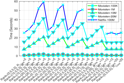
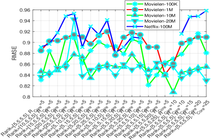
Refer to caption
(a) Computational Time
Refer to caption
(b) RMSE
Figure 7: Computational overhead, RMSE, and MAE VS. various rank values for SGD__\_Tucker on 8 Cores. Due to limited space, each dataset is presented in 444-order. As Netflix-100M data set only has 333-order, its 4th index shall be neglected.
Refer to caption
(a) Movielen-10M
Refer to caption
(b) Movielen-20M
Refer to caption
(c) Netflix-100M
Refer to caption
(d) Yahoo-250M
Figure 8: RMSE and MAE vs time for SGD__\_Tucker on training set ΩΩ\Omega and testing set ΓΓ\Gamma
Refer to caption
(a) Movielen-10M
Refer to caption
(b) Movielen-20M
Refer to caption
(c) Netflix-100M
Refer to caption
(d) Yahoo-250M
Figure 9: RMSE comparison of SGD__\_Tucker, P-Tucker, and CD on the 4 datasets.
Refer to caption
Figure 10: Speedup Performance on the 6 datasets.

5.1 Experimental Settings

The CPU server is equipped with 8 Intel(R) Xeon(R) E5-2620 v4 CPUs and each core has 2 hyperthreads, running on 2.10 GHz, for the state of the art algorithms for STD, e.g., P-Tucker [46], CD [47] and HOOI [41]. The experiments are conducted 3 public datasets : Netflix 111https://www.netflixprize.com/ , Movielens 222https://grouplens.org/datasets/movielens/ , and Yahoo-music 333https://webscope.sandbox.yahoo.com/catalog.php?datatype . The datasets which be used in our experiments can be downloaded in this link. 444https://drive.google.com/drive/folders/1tcnAsUSC9jFty7AfWetb5R
7nevN2WUxH?usp=sharing
For Movielens, data cleaning is conducted and 00 values are changed from zero to 0.50.50.5 and we make compression for Yahoo-music dataset in which the maximum value 100 be compressed to 5.0. The specific situation of datasets is shown in Table III. In this way, the ratings of the two data sets are in the same interval, which facilitates the selection of parameters. Gaussian distribution N(0.5,0.12)𝑁0.5superscript0.12N\bigg{(}0.5,0.1^{2}\bigg{)} is adopted for initialization; meanwhile, the regularization parameters {λA,λB}subscript𝜆Asubscript𝜆B\{\lambda_{\textbf{A}},\lambda_{\textbf{B}}\} are set as 0.010.010.01 and the learning rate {γA,γB}subscript𝛾Asubscript𝛾B\{\gamma_{\textbf{A}},\gamma_{\textbf{B}}\} are set as {0.002,0.001}0.0020.001\{0.002,0.001\}, respectively. For simplification, we set M=1𝑀1M=1. The accuracy is measured by RMSE𝑅𝑀𝑆𝐸RMSE and MAE𝑀𝐴𝐸MAE as:

RMSE𝑅𝑀𝑆𝐸\displaystyle RMSE =((i1,,iN)Γ(xi1,,iNx^i1,,iN)2)/|Γ|;absentsubscriptsubscript𝑖1subscript𝑖𝑁Γsuperscriptsubscript𝑥subscript𝑖1subscript𝑖𝑁subscript^𝑥subscript𝑖1subscript𝑖𝑁2Γ\displaystyle=\sqrt{\bigg{(}\sum_{(i_{1},\cdots,i_{N})\in\Gamma}(x_{i_{1},\cdots,i_{N}}-\widehat{x}_{i_{1},\cdots,i_{N}})^{2}\bigg{)}\bigg{/}|\Gamma|}; (19)
MAE𝑀𝐴𝐸\displaystyle MAE =((i1,,iN)Γ|xi1,,iNx^i1,,iN|)/|Γ|,absentsubscriptsubscript𝑖1subscript𝑖𝑁Γsubscript𝑥subscript𝑖1subscript𝑖𝑁subscript^𝑥subscript𝑖1subscript𝑖𝑁Γ\displaystyle=\bigg{(}\sum_{(i_{1},\cdots,i_{N})\in\Gamma}\bigg{|}x_{i_{1},\cdots,i_{N}}-\widehat{x}_{i_{1},\cdots,i_{N}}\bigg{|}\bigg{)}\bigg{/}|\Gamma|,

respectively, where ΓΓ\Gamma denotes the test sets. All the experiments are conducted on double-precision float numeric.

5.2 Scalability of the Approach

When ML algorithms process large-scale data, two factors to influence the computational overhead are: 1) time spent for data access on memory, i.e., reading and writing data; 2) time spent on the computational components for executing the ML algorithms. Fig. 5 presents the computational overhead per training epoch. The codes of P-Tucker and CD have fixed settings for the rank value, i.e., J1==Jn==JNsubscript𝐽1subscript𝐽𝑛subscript𝐽𝑁J_{1}=\cdots=J_{n}=\cdots=J_{N}. The rank value is set as an increasing order, {3,5,7,9,11}357911\{3,5,7,9,11\}. As shown in Fig. 5, SGD__\_Tucker has the lowest computational time overhead. HOOI needs to construct the intermediate matrices Y(n)subscriptY𝑛\textbf{Y}_{(n)} \in In×knNJksuperscriptsubscript𝐼𝑛superscriptsubscriptproduct𝑘𝑛𝑁subscript𝐽𝑘\mathbb{R}^{I_{n}\times\prod\limits_{k\neq n}^{N}J_{k}}, n𝑛n \in {N}𝑁\{N\} and SVD for Y(n)subscriptY𝑛\textbf{Y}_{(n)} (In supplementary material). P-Tucker should construct Hessian matrix and the computational complexity of each Hessian matrix inversion is O(Jn3)𝑂superscriptsubscript𝐽𝑛3O\big{(}J_{n}^{3}\big{)}, n𝑛n \in {N}𝑁\{N\}. P-Tucker saves the memory overhead a lot at the expense of adding the memory accessing overhead. Eventually, the accessing and computational overheads for inverse operations of Hessian matrices make the overall computational time of P-Tucker surpass SGD__\_Tucker. The computational structure of CD has linear scalability. However, the CD makes the update process of each feature element in a feature vector be discrete. Thus, the addressing process is time-consuming. Meanwhile, as Fig. 5 shows, the computational overhead satisfies the constraints of the time complexity analyses, i.e., P-Tucker, HOOI, CD (Supplementary material) and SGD__\_Tucker (Section 4.5).

The main space overheads for STD comes from the storage need of the intermediate matrices. The SVD operation for the intermediate matrices Y(n)subscriptY𝑛\textbf{Y}_{(n)} \in In×knNJksuperscriptsubscript𝐼𝑛superscriptsubscriptproduct𝑘𝑛𝑁subscript𝐽𝑘\mathbb{R}^{I_{n}\times\prod\limits_{k\neq n}^{N}J_{k}}, n𝑛n \in {N}𝑁\{N\} makes the HOOI scale exponentially. P-Tucker constructs the eventual Hessian matrices directly which can avoid the huge construction of intermediate matrices. However, the overhead for addressing is huge and the long time-consuming for CD lies in the same situation. CD is a linear approach from the update equation (Supplementary material). However, in reality, the linearity comes from the approximation of the second-order Hessian matrices and, thus, the accessing overhead of discrete elements of CD overwhelms the accessing overhead of continuous ones (P-Tucker and SGD__\_Tucker). As shown in Fig. 6, SGD__\_Tucker has linear scalability for space overhead and HOOI is exponentially scalable. P-Tucker and CD have the near-linear space overhead. However, as Fig. 5 shows, the computational overheads of P-Tucker and CD is significantly higher than SGD__\_Tucker. Meanwhile, as Fig. 6 shows, the space overhead satisfies the constraints of the space complexity analyses, i.e., HOOI, P-Tucker, and CD (Supplementary material) and SGD__\_Tucker (Section 4.5).

5.3 The Influence of Parameters

In this section, the influence of the rank on the behavior of the algorithm is presented. We summarize the influence on the computational time and the RMSE are presented in Fig. 7. The Netflix-100M dataset has only 3-order. Owing to the limited space, the performances on Netflix-100M dataset are combined with other 5 datasets (Netflix-100M dataset has only 3-order and the performances on the 4th order of Netflix-100M dataset should be negligible). The update for the Kruskal matrices B(n)superscriptB𝑛\textbf{B}^{(n)}, n𝑛n \in N𝑁N on the steps of beginning and last epochs can also obtain a comparable results. Thus, the presentation for the Kruskal matrices B(n)superscriptB𝑛\textbf{B}^{(n)}, n𝑛n \in N𝑁N is omitted. The influence for computational time is divided into 5 sets, i.e., {J1{5,10,15,20,25},Jk=5,k1,RCore=5}formulae-sequencesubscript𝐽1510152025formulae-sequencesubscript𝐽𝑘5formulae-sequence𝑘1subscript𝑅𝐶𝑜𝑟𝑒5\big{\{}J_{1}\in\{5,10,15,20,25\},J_{k}=5,k\neq 1,R_{Core}=5\big{\}}, {J2{5,10,15,20,25},Jk=5,k2,RCore=5}formulae-sequencesubscript𝐽2510152025formulae-sequencesubscript𝐽𝑘5formulae-sequence𝑘2subscript𝑅𝐶𝑜𝑟𝑒5\big{\{}J_{2}\in\{5,10,15,20,25\},J_{k}=5,k\neq 2,R_{Core}=5\big{\}}, {J3{5,10,15,20,25},Jk=5,k3,RCore=5}formulae-sequencesubscript𝐽3510152025formulae-sequencesubscript𝐽𝑘5formulae-sequence𝑘3subscript𝑅𝐶𝑜𝑟𝑒5\big{\{}J_{3}\in\{5,10,15,20,25\},J_{k}=5,k\neq 3,R_{Core}=5\big{\}}, {J4{5,10,15,20,25},Jk=5,k4,RCore=5}formulae-sequencesubscript𝐽4510152025formulae-sequencesubscript𝐽𝑘5formulae-sequence𝑘4subscript𝑅𝐶𝑜𝑟𝑒5\big{\{}J_{4}\in\{5,10,15,20,25\},J_{k}=5,k\neq 4,R_{Core}=5\big{\}}, {Jn=5,n{N},RCore{10,15,20,25}}formulae-sequencesubscript𝐽𝑛5formulae-sequence𝑛𝑁subscript𝑅𝐶𝑜𝑟𝑒10152025\big{\{}J_{n}=5,n\in\{N\},R_{Core}\in\{10,15,20,25\}\big{\}}. As the Fig. 7 (a) shows, the computation time increases with Jnsubscript𝐽𝑛J_{n}, n𝑛n \in {N}𝑁\{N\} increasing linearly and the RCoresubscript𝑅𝐶𝑜𝑟𝑒R_{Core} only has slight influence for computational time.

The codes of P-Tucker and CD have fixed settings for the rank value (J1==Jn==JNsubscript𝐽1subscript𝐽𝑛subscript𝐽𝑁J_{1}=\cdots=J_{n}=\cdots=J_{N}). For a fair comparison, the rank values that we select should have slight changes with the RMSE performances of other rank values. The computational overhead of P-Tucker and CD is sensitive to the rank value and RMSE is comparable non-sensitive. Hence, we choose a slightly small value Jn=5|n{N}subscript𝐽𝑛conditional5𝑛𝑁J_{n}=5|n\in\{N\}. As Fig. 7 (b) shows, when rank is set as Jn=5,n{N}formulae-sequencesubscript𝐽𝑛5𝑛𝑁J_{n}=5,n\in\{N\}, the RMSE is equivalent to other situations on average.

5.4 Speedup and Comparisons

We test the RMSE performances on the 6 datasets and the RMSE is used to estimate the missing entries. The speedup is evaluated as Time1/TimeT𝑇𝑖𝑚subscript𝑒1𝑇𝑖𝑚subscript𝑒𝑇Time_{1}/Time_{T} where TimeT𝑇𝑖𝑚subscript𝑒𝑇Time_{T} is the running time with T𝑇T threads. When T𝑇T == {1,,8}18\{1,\cdots,8\}, as the Fig. 10 shows, the speedup performance of SGD__\_Tucker has a near-linear speedup. The speedup performance is presented in Fig. 10 which shows the whole speedup performance of the SGD__\_Tucker. The speedup performance is a bit more slower when the number of threads is larger than 888. The reason is that the thread scheduling and synchronization occupies a large part of time. When we use 161616 threads, there is still a 11X11𝑋11X speedup and the efficiency is 11/16=68%1116percent6811/16=68\%.

The rank value for 333-order tensor is set to [5,5,5]555[5,5,5] and the rank value for 444-order tensor is set to [5,5,5,5]5555[5,5,5,5]. To demonstrate the convergence of SGD__\_Tucker, the convergence performances of SGD__\_Tucker for the Movielen and Netflix are presented in Fig. 8. As shown in Fig. 8, SGD__\_Tucker can get more stable RMSE and MAE metrices which mean that SGD__\_Tucker has more robustness in large-scale datasets than in small datasets. As Fig. 9 shows, SGD__\_Tucker can not only run faster than the state of the art approaches, i.e., P-Tucker and CD, but also can obtain higher RMSE value. SGE__\_Tucker runs 2X𝑋X and 20X𝑋X faster than P-Tucker and CD, respectively, to obtain the optimal RMSE value.

6 Conclusion and Future Works

STD is widely used in low-rank representation learning for sparse big data analysis. Due to the entanglement problem of core tensor and factor matrices, the computational process for STD has the intermediate variables explosion problem due to following all elements in HOHDST. To solve this problem, we first derive novel optimization objection function for STD and then propose SGD__\_Tucker to solve it by dividing the high-dimension intermediate variables into small batches of intermediate matrices. Meanwhile, the low data-dependence of SGD__\_Tucker makes it amenable to fine-grained parallelization. The experimental results show that SGD__\_Tucker has linear computational time and space overheads and SGD__\_Tucker runs at least 2X𝑋X faster than the state of the art STD solutions. In the future works, we plan to explore how to accelerate the SGD__\_Tucker by the state of the art stochastic models, e.g., variance SGD [32], Stochastic Recursive Gradient [34], or momentum SGD [35].

SGD__\_Tucker is a linearly scalable method for STD on big-data platforms. For the future work, we will embed SGD__\_Tucker into popular distributed data processing platforms such as Hadoop, Spark, or Flink. We will also aim to extend SGD__\_Tucker to GPU platforms, i.e., OpenCL and CUDA.

Acknowledgement

References

  • [1] A. Cichocki, N. Lee, I. Oseledets, A.-H. Phan, Q. Zhao, and D. P. Mandic, “Tensor networks for dimensionality reduction and large-scale optimization: Part 1 low-rank tensor decompositions,” Foundations and Trends® in Machine Learning, vol. 9, no. 4-5, pp. 249–429, 2016.
  • [2] V. N. Ioannidis, A. S. Zamzam, G. B. Giannakis, and N. D. Sidiropoulos, “Coupled graph and tensor factorization for recommender systems and community detection,” IEEE Transactions on Knowledge and Data Engineering, 2019.
  • [3] X. Luo, H. Wu, H. Yuan, and M. Zhou, “Temporal pattern-aware qos prediction via biased non-negative latent factorization of tensors,” IEEE transactions on cybernetics, 2019.
  • [4] K. Xie, X. Li, X. Wang, G. Xie, J. Wen, and D. Zhang, “Active sparse mobile crowd sensing based on matrix completion,” in Proceedings of the International Conference on Management of Data, 2019, pp. 195–210.
  • [5] X. Wang, L. T. Yang, X. Xie, J. Jin, and M. J. Deen, “A cloud-edge computing framework for cyber-physical-social services,” IEEE Communications Magazine, vol. 55, no. 11, pp. 80–85, 2017.
  • [6] P. Wang, L. T. Yang, G. Qian, J. Li, and Z. Yan, “Ho-otsvd: A novel tensor decomposition and its incremental decomposition for cyber-physical-social networks (cpsn),” IEEE Transactions on Network Science and Engineering, 2019.
  • [7] T. Wang, X. Xu, Y. Yang, A. Hanjalic, H. T. Shen, and J. Song, “Matching images and text with multi-modal tensor fusion and re-ranking,” in Proceedings of the 27th ACM international conference on multimedia.   ACM, 2019, pp. 12–20.
  • [8] M. Hou, J. Tang, J. Zhang, W. Kong, and Q. Zhao, “Deep multimodal multilinear fusion with high-order polynomial pooling,” in Advances in Neural Information Processing Systems, 2019, pp. 12 113–12 122.
  • [9] P. P. Liang, Z. Liu, Y.-H. H. Tsai, Q. Zhao, R. Salakhutdinov, and L.-P. Morency, “Learning representations from imperfect time series data via tensor rank regularization,” in Proceedings of the Annual Meeting of the Association for Computational Linguistics, 2019.
  • [10] Y. Liu, L. He, B. Cao, S. Y. Philip, A. B. Ragin, and A. D. Leow, “Multi-view multi-graph embedding for brain network clustering analysis,” in AAAI Conference on Artificial Intelligence, 2018.
  • [11] A. Cichocki, A. Phan, I. Oseledets, Q. Zhao, M. Sugiyama, N. Lee, and D. Mandic, “Tensor networks for dimensionality reduction and large-scale optimizations: Part 2 applications and future perspectives,” Foundations and Trends in Machine Learning, vol. 9, no. 6, pp. 431–673, 2017.
  • [12] L. Van Der Maaten, E. Postma, and J. Van den Herik, “Dimensionality reduction: a comparative,” Journal of Machine Learning Research, vol. 10, no. 66-71, p. 13, 2009.
  • [13] J. Xu, J. Zhou, P.-N. Tan, X. Liu, and L. Luo, “Spatio-temporal multi-task learning via tensor decomposition,” IEEE Transactions on Knowledge and Data Engineering, 2019.
  • [14] X. Liu, X. You, X. Zhang, J. Wu, and P. Lv, “Tensor graph convolutional networks for text classification,” arXiv preprint arXiv:2001.05313, 2020.
  • [15] M. Abadi, P. Barham, J. Chen, Z. Chen, A. Davis, J. Dean, M. Devin, S. Ghemawat, G. Irving, M. Isard et al., “Tensorflow: A system for large-scale machine learning,” in {{\{USENIX}}\} Symposium on Operating Systems Design and Implementation ({{\{OSDI}}\}), 2016, pp. 265–283.
  • [16] J. Kossaifi, A. Bulat, G. Tzimiropoulos, and M. Pantic, “T-net: Parametrizing fully convolutional nets with a single high-order tensor,” in Proceedings of the IEEE Conference on Computer Vision and Pattern Recognition, 2019, pp. 7822–7831.
  • [17] F. Ju, Y. Sun, J. Gao, M. Antolovich, J. Dong, and B. Yin, “Tensorizing restricted boltzmann machine,” ACM Transactions on Knowledge Discovery from Data, vol. 13, no. 3, pp. 1–16, 2019.
  • [18] M. Wang, Z. Shu, S. Cheng, Y. Panagakis, D. Samaras, and S. Zafeiriou, “An adversarial neuro-tensorial approach for learning disentangled representations,” International Journal of Computer Vision, vol. 127, no. 6-7, pp. 743–762, 2019.
  • [19] C. Zhang, H. Fu, J. Wang, W. Li, X. Cao, and Q. Hu, “Tensorized multi-view subspace representation learning,” International Journal of Computer Vision, pp. 1–18, 2020.
  • [20] Y. Luo, D. Tao, K. Ramamohanarao, C. Xu, and Y. Wen, “Tensor canonical correlation analysis for multi-view dimension reduction,” IEEE transactions on Knowledge and Data Engineering, vol. 27, no. 11, pp. 3111–3124, 2015.
  • [21] X. Liu, X. Zhu, M. Li, L. Wang, E. Zhu, T. Liu, M. Kloft, D. Shen, J. Yin, and W. Gao, “Multiple kernel k-means with incomplete kernels,” IEEE transactions on pattern analysis and machine intelligence, 2019.
  • [22] P. Symeonidis, A. Nanopoulos, and Y. Manolopoulos, “Tag recommendations based on tensor dimensionality reduction,” in Proceedings of the ACM conference on Recommender systems, 2008, pp. 43–50.
  • [23] I. Balazevic, C. Allen, and T. Hospedales, “Tucker: Tensor factorization for knowledge graph completion,” in Proceedings of the Conference on Empirical Methods in Natural Language Processing and the 9th International Joint Conference on Natural Language Processing (EMNLP-IJCNLP), 2019, pp. 5188–5197.
  • [24] J. Liu, P. Musialski, P. Wonka, and J. Ye, “Tensor completion for estimating missing values in visual data,” IEEE transactions on pattern analysis and machine intelligence, vol. 35, no. 1, pp. 208–220, 2012.
  • [25] S. Zubair and W. Wang, “Tensor dictionary learning with sparse tucker decomposition,” in International Conference on Digital Signal Processing.   IEEE, 2013, pp. 1–6.
  • [26] S. Oh, N. Park, S. Lee, and U. Kang, “Scalable tucker factorization for sparse tensors-algorithms and discoveries,” in IEEE International Conference on Data Engineering.   IEEE, 2018, pp. 1120–1131.
  • [27] V. T. Chakaravarthy, J. W. Choi, D. J. Joseph, P. Murali, S. S. Pandian, Y. Sabharwal, and D. Sreedhar, “On optimizing distributed tucker decomposition for sparse tensors,” in Proceedings of the International Conference on Supercomputing, 2018, pp. 374–384.
  • [28] B. N. Sheehan and Y. Saad, “Higher order orthogonal iteration of tensors (hooi) and its relation to pca and glram,” in Proceedings of the SIAM International Conference on Data Mining.   SIAM, 2007, pp. 355–365.
  • [29] A. Kulunchakov and J. Mairal, “A generic acceleration framework for stochastic composite optimization,” in Advances in Neural Information Processing Systems, 2019, pp. 12 556–12 567.
  • [30] A. Traoré, M. Berar, and A. Rakotomamonjy, “Singleshot: a scalable tucker tensor decomposition,” in Advances in Neural Information Processing Systems, 2019, pp. 6301–6312.
  • [31] O. A. Malik and S. Becker, “Low-rank tucker decomposition of large tensors using tensorsketch,” in Advances in Neural Information Processing Systems, 2018, pp. 10 096–10 106.
  • [32] R. Johnson and T. Zhang, “Accelerating stochastic gradient descent using predictive variance reduction,” in Advances in neural information processing systems, 2013, pp. 315–323.
  • [33] M. Schmidt, N. Le Roux, and F. Bach, “Minimizing finite sums with the stochastic average gradient,” Mathematical Programming, vol. 162, no. 1-2, pp. 83–112, 2017.
  • [34] L. M. Nguyen, J. Liu, K. Scheinberg, and M. Takáč, “Sarah: A novel method for machine learning problems using stochastic recursive gradient,” in Proceedings of the International Conference on Machine Learning.   JMLR. org, 2017, pp. 2613–2621.
  • [35] H. Yu, R. Jin, and S. Yang, “On the linear speedup analysis of communication efficient momentum sgd for distributed non-convex optimization,” in International Conference on Machine Learning, 2019, pp. 7184–7193.
  • [36] S. Shalev-Shwartz et al., “Online learning and online convex optimization,” Foundations and Trends in Machine Learning, vol. 4, no. 2, pp. 107–194, 2012.
  • [37] N. Ketkar, “Introduction to pytorch,” in Deep learning with python.   Springer, 2017, pp. 195–208.
  • [38] J. Verbraeken, M. Wolting, J. Katzy, J. Kloppenburg, T. Verbelen, and J. S. Rellermeyer, “A survey on distributed machine learning,” ACM Computing Survey, vol. 53, no. 2, Mar. 2020.
  • [39] S. Dutta, G. Joshi, S. Ghosh, P. Dube, and P. Nagpurkar, “Slow and stale gradients can win the race: Error-runtime trade-offs in distributed sgd,” in International Conference on Artificial Intelligence and Statistics, 2018, pp. 803–812.
  • [40] H. Ge, K. Zhang, M. Alfifi, X. Hu, and J. Caverlee, “Distenc: A distributed algorithm for scalable tensor completion on spark,” in 2018 IEEE International Conference on Data Engineering.   IEEE, 2018, pp. 137–148.
  • [41] S. Smith and G. Karypis, “Accelerating the tucker decomposition with compressed sparse tensors,” in European Conference on Parallel Processing.   Springer, 2017, pp. 653–668.
  • [42] Y. Ma, J. Li, X. Wu, C. Yan, J. Sun, and R. Vuduc, “Optimizing sparse tensor times matrix on gpus,” Journal of Parallel and Distributed Computing, vol. 129, pp. 99–109, 2019.
  • [43] V. T. Chakaravarthy, S. S. Pandian, S. Raje, and Y. Sabharwal, “On optimizing distributed non-negative tucker decomposition,” in Proceedings of the ACM International Conference on Supercomputing, 2019, pp. 238–249.
  • [44] O. Kaya and B. Uçar, “High performance parallel algorithms for the tucker decomposition of sparse tensors,” in 2016 45th International Conference on Parallel Processing (ICPP).   IEEE, 2016, pp. 103–112.
  • [45] V. T. Chakaravarthy, J. W. Choi, D. J. Joseph, P. Murali, S. S. Pandian, Y. Sabharwal, and D. Sreedhar, “On optimizing distributed tucker decomposition for sparse tensors,” in Proceedings of the International Conference on Supercomputing, 2018, pp. 374–384.
  • [46] S. Oh, N. Park, S. Lee, and U. Kang, “Scalable tucker factorization for sparse tensors-algorithms and discoveries,” in IEEE International Conference on Data Engineering (ICDE).   IEEE, 2018, pp. 1120–1131.
  • [47] M. Park, J.-G. Jang, and S. Lee, “Vest: Very sparse tucker factorization of large-scale tensors,” arXiv preprint arXiv:1904.02603, 2019.
  • [48] S. Oh, N. Park, J.-G. Jang, L. Sael, and U. Kang, “High-performance tucker factorization on heterogeneous platforms,” IEEE Transactions on Parallel and Distributed Systems, vol. 30, no. 10, pp. 2237–2248, 2019.
  • [49] Y. Nesterov, Introductory lectures on convex optimization: A basic course.   Springer Science & Business Media, 2013, vol. 87.
  • [50] Y. Chi, Y. M. Lu, and Y. Chen, “Nonconvex optimization meets low-rank matrix factorization: An overview,” IEEE Transactions on Signal Processing, vol. 67, no. 20, pp. 5239–5269, 2019.
  • [51] Y. Xu and W. Yin, “A block coordinate descent method for regularized multiconvex optimization with applications to nonnegative tensor factorization and completion,” SIAM Journal on imaging sciences, vol. 6, no. 3, pp. 1758–1789, 2013.
  • [52] S. Boyd, S. P. Boyd, and L. Vandenberghe, Convex optimization.   Cambridge university press, 2004.
  • [53] H. Li, C. Fang, and Z. Lin, “Accelerated first-order optimization algorithms for machine learning,” Proceedings of the IEEE, 2020.
  • [54] S. J. Reddi, A. Hefny, S. Sra, B. Poczos, and A. Smola, “Stochastic variance reduction for nonconvex optimization,” in International conference on machine learning, 2016, pp. 314–323.
  • [55] H. Li, K. Li, J. An, and K. Li, “Msgd: A novel matrix factorization approach for large-scale collaborative filtering recommender systems on gpus,” IEEE Transactions on Parallel and Distributed Systems, vol. 29, no. 7, pp. 1530–1544, 2017.