Non-parametric Quantile Regression via the K-NN Fused Lasso

Abstract

Quantile regression is a statistical method for estimating conditional quantiles of a response variable. In addition, for mean estimation, it is well known that quantile regression is more robust to outliers than $l_{2}$-based methods. By using the fused lasso penalty over a $K$-nearest neighbors graph, we propose an adaptive quantile estimator in a non-parametric setup. We show that the estimator attains optimal rate of $n^{-1/d}$ up to a logarithmic factor, under mild assumptions on the data generation mechanism of the $d$-dimensional data. We develop algorithms to compute the estimator and discuss methodology for model selection. Numerical experiments on simulated and real data demonstrate clear advantages of the proposed estimator over state of the art methods. All codes that implement the algorithms and the datasets used in the experiments are publicly available on the author’s Github page (https://github.com/stevenysw/qt_knnfl).

Keywords: quantile regression, non-parametric, fused lasso, $K$-nearest neighbors, bounded variation

1 Introduction

Assume that we have $n$ observations, $(x_{1},y_{1}),...,(x_{n},y_{n}),$ of the pair of random variables $(X,Y)$. The response variable $Y$ is a real-valued vector and $X$ is a multivariate covariate or predictor variable in a metric space $\mathcal{X}$ with metric $d_{\mathcal{X}}$. A standard goal of non-parametric regression is to infer, in some way, the underlying relationship between $Y$ and $X$. The generative model behind this can be expressed as

$$y_{i}=f_{0}(x_{i})+\epsilon_{i},\ \text{for }i=1,...,n,$$ (1)

where $f_{0}$ is an unknown function that we want to estimate. While usual regression considers estimation of the conditional mean of the response variable, quantile regression estimates the conditional median (or other desired quantiles) of the response variable. Specifically, given a quantile level $\tau\in(0,1)$, we can rewrite (1) as

$$y_{i}=\theta^{\ast}_{i}+\epsilon_{i},\ \text{for }i=1,...,n,$$ (2)

where

$$\theta^{\ast}_{i}=F^{-1}_{y_{i}|x_{i}}(\tau).$$ (3)

Here, $\theta^{\ast}$ is the vector of $\tau$-quantiles of $y$, $F_{y_{i}|x_{i}}$ represents the cumulative distribution function of $y_{i}$ given $x_{i}$, and $\mathbb{P}(\epsilon_{i}\leq 0|x_{i})=\tau$.

The goal of quantile regression is to estimate $\theta^{\ast}$ as accurately as possible, and it usually involves an optimization problem in the form

$$\hat{\theta}\in\underset{\theta\in\zeta\subset\mathbb{R}^{n}}{\arg\min}\ L(\theta),$$ (4)

where $L(\theta)$ is the loss function is defined by

$$L(\theta)=\sum_{i=1}^{n}\rho_{\tau}(y_{i}-\theta_{i}),$$ (5)

with $\rho_{\tau}(t)=(\tau-1\{t\leq 0\})t$, the asymmetric absolute deviation function (Koenker and Bassett Jr, 1978).

In this paper, we apply total variation denoising for non-parametric quantile regression in a multivariate setup and combine it with the $K$-NN procedure. We leverage insights gained from recent results for quantile trend filtering (Padilla and Chatterjee, 2020) and $K$-NN fused lasso (Padilla et al., 2020a). Our proposed estimator, quantile $K$-NN fused lasso, can adapt to the piecewise linear or piecewise polynomial structure in the true vector properly.

It takes simply two steps to compute our proposed quantile $K$-NN fused lasso estimator. We first construct a $K$-nearest-neighbor graph corresponding to the given observations. The second step involves a constrained optimization problem with a lasso-type penalty along the $K$-NN graph as follow

$$\hat{\theta}\in\underset{\theta\in\zeta\subset\mathbb{R}^{n}}{\arg\min}\ L(\theta)+\lambda\|\nabla_{G}\theta\|_{1},$$ (6)

where $\lambda>0$ is a tuning parameter. The notation $\nabla_{G}$ in the penalty term represents the oriented incidence matrix of the $K$-NN graph, and we will provide the detailed definition in Section 2.

We study the rate of convergence of the estimator defined in (6). Towards that end, we denote a loss function $\Delta_{n}^{2}:\mathbb{R}^{n}\rightarrow\mathbb{R}$ by

$$\Delta_{n}^{2}(\delta):=\frac{1}{n}\sum_{i=1}^{n}\min\{|\delta_{i}|,\delta_{i}^{2}\}.$$

The function $\Delta_{n}^{2}(\cdot)$ appeared in Padilla and Chatterjee (2020) and is similar to a Huber loss function (see page 471 in Wainwright, 2018), which offers a compromise between the least-squares cost and the $l_{1}$-norm cost function and is thus less sensitive to outliers in data. We show that under mild conditions, (6) attains a convergence rate of $n^{-1/d}$ for $d$-dimensional data in terms of $\Delta_{n}^{2}$, ignoring the logarithmic factor. The rate is nearly minimax and it matches the mean squared error rates from Padilla et al. (2020a). However, unlike Padilla et al. (2020a), our result holds under general errors allowing for heavy-tailed distributions. Another notable point in our theoretical analysis, different from previous quantile regression work, is that we only require a bounded variation class of signals and hence guarantee our result to hold under very general models.

1.1 Previous Work

Quantile regression, since introduced by Koenker and Bassett Jr (1978), has become a commonly used class of methods in many applications thanks to its flexibility and robustness for modelling conditional distributions. The study of quantile regression in non-parametric setups can be dated back to Utreras (1981), Cox (1983) and Eubank (1988), whose works were mainly developed for median regression on one-dimensional data. Later, Koenker et al. (1994) proposed a more general estimator for any desired quantile $\tau$, quantile smoothing spline, and He et al. (1998) provided a bivariate version of the estimator. Quantile smoothing spline problems are of a $l_{1}$ penalty structure, which led to a more general study on $l_{1}$-norm regularized quantile regression by Li and Zhu (2008). Other methods for non-parametric quantile regression have also been proposed in the literature. Yu and Jones (1998), Cai and Xu (2008), and Spokoiny et al. (2013) explored local polynomial quantile regression. Belloni et al. (2019) studied non-parametric series quantile regression, and Meinshausen (2006) introduced quantile random forests. Quantile regression with rectified linear unit (ReLU) neural networks is another edge-cutting approach that utilizes some knowledge from the field of deep learning, and the theory is studied in Padilla et al. (2020b).

Our approach exploits the local adaptivity of total variation denoising. Rudin et al. (1992) first proposed total variation denoising for the application of image processing, and Tibshirani and Saunders (2005) studied fused lasso thoroughly. Later, Kim et al. (2009) extended the discussion to the so-called trend filtering on one-dimensional data, and Wang et al. (2016) provided a generalization of trend filtering to the setting of estimation on graphs. These problems can be formulated similarly into an optimization problem of the form

$$\hat{\theta}\in\underset{\theta\in\mathbb{R}^{n}}{\arg\min}\ \frac{1}{2}\sum_{i=1}^{n}(\theta_{i}-y_{i})^{2}+\lambda\|D\theta\|_{1},$$ (7)

where $\lambda>0$ is a regularization parameter to be chosen carefully and $D$ is a matrix. For instance, trend filtering order $k$ (fused lasso $k=0$) consists of matrices $D$ that capture the $(k+1)$th order total variation of a given signal, see Tibshirani (2014). A substantial amount of literature focused on theoretical guarantees of these estimators. Mammen and van de Geer (1997) and Tibshirani (2014) showed that trend filtering attains nearly minimax rates in mean squared error (MSE) for estimating functions of bounded variation. Hütter and Rigollet (2016) showed a sharp oracle rate of total variation denoising along grid graphs. More recently, Padilla et al. (2020a) incorporated fused lasso with the $K$-NN procedure and proved that the $K$-NN fused lasso also achieves nearly minimax convergence rate. In the quantile regression literature, Belloni and Chernozhukov (2011), Kato (2011), Fan et al. (2014) studied quantile model selection via $l_{1}$ regularization, but most of these works required strict linear assumptions. Padilla and Chatterjee (2020) provided proofs for theoretical properties of quantile trend filtering estimator in one dimension. They showed that under minimal assumptions of the data generation mechanism, quantile trend filtering estimator attains a minimax rate for one-dimensional piecewise polynomial regression.

On the computational side, quantile regression is different from $l_{2}$ based methods because it requires a non-trivial reformulation of the optimization problem due to non-differentiability of the loss as (5). The most well-known algorithm for computing a quantile estimator is due to Koenker (2005) and it uses an interior point (IP) approach. Pietrosanu et al. (2017) studied high-dimensional quantile regression problems and obtained estimators by applying the alternating direction method of multipliers (ADMM; Boyd et al., 2011), majorize-minimize (MM; Hunter and Lange, 2000), and coordinate descent (CD; Wu and Lange, 2008) algorithms for variable selection. For computing trend filtering estimates, Hochbaum and Lu (2017) developed a fast algorithm for quantile fused lasso in $O(n\log n)$ operations. Recently, Brantley et al. (2020) proposed an ADMM based algorithm for computing $k$th order quantile trend filtering estimators for one-dimensional data.

1.2 Outline of the Paper

In Section 2, we provide the definition of quantile $K$-nearest-neighbors fused lasso estimator and the constrained version of the problem. Two algorithms to compute the proposed estimators numerically – alternating directions method of multipliers (ADMM), and majorize-minimize (MM), are introduced in Section 3, and the discussion on how to select an appropriate penalty parameter in practice is also included. Section 4 presents the two theoretical developments regarding the constrained and penalized estimators. The theorems demonstrate that under general assumptions, both estimators converge at a rate of $n^{-1/d}$, up to a logarithmic factor, for estimating $d$-dimensional data under the loss function $\Delta^{2}_{n}$ defined above. Section 5 lists the results of numerical experiments on multiple simulated datasets and two real datasets, California housing data and Chicago crime data. The experiments show that the proposed estimator outperform state-of-the-art methods on both simulated and real datasets. Moreover, the comparison on accuracy and computational time among the algorithms introduced in Section 3 provides the audience with some insights on choosing a suitable algorithm for specific problems. The proofs of theorems in the paper are provided in the Appendix.

2 Quantile K-NN Fused Lasso

The first step to construct the quantile $K$-NN fused lasso estimator is to build a $K$-NN graph $G$. Specifically, given the observations, $G$ has vertex set $V=\{1,...,n\}$, and its edge set $E_{K}$ contains the pair $(i,j)$, for $i\in V$, $j\in V$, and $i\neq j$, if and only if $x_{i}$ is among the $K$-nearest neighbors of $x_{j}$, with respect to the metric $d_{\mathcal{X}}$, or vice versa. After constructing the $K$-NN graph, we can formalize an optimization problem for quantile $K$-NN fused lasso as

$$\hat{\theta}=\underset{\theta\in\mathbb{R}^{n}}{\arg\min}\ \sum_{i=1}^{n}\rho_{\tau}(y_{i}-\theta_{i})+\lambda\|\nabla_{G}\theta\|_{1},$$ (8)

where $\lambda>0$ is a tuning parameter, and $\nabla_{G}$ is an oriented incidence matrix of the $K$-NN graph $G$. Thus, we define $\nabla_{G}$ as follows: each row of the matrix corresponds to one edge in $G$; for instance, if the $p$-th edge in $G$ connects the $i$-th and $j$-th observations, then

$$\left(\nabla_{G}\right)_{p,q}=\begin{cases}1&\text{if }q=i,\\ -1&\text{if }q=j,\\ 0&\text{otherwise.}\end{cases}$$

In this way, the $p$-th element in $\nabla_{G}\theta$, $(\nabla_{G}\theta)_{p}=\theta_{i}-\theta_{j}$. Notice that we choose the ordering of the nodes and edges in $\nabla_{G}$ arbitrarily without loss of generality.

Once $\hat{\theta}$ in (8) has been computed, we can predict the value of response corresponding to a new observation $x\in\mathcal{X}\backslash\{x_{1},...,x_{n}\}$ by the averaged estimated response of the $K$-nearest neighbors of $x$ in $\{x_{1},...,x_{n}\}$. Mathematically, we write

$$\hat{y}=\frac{1}{K}\sum_{i=1}^{n}\hat{\theta}_{i}\cdot\textbf{1}\{x_{i}\in\mathcal{N}_{K}(x)\},$$ (9)

where $\mathcal{N}_{K}(x)$ is the set of $K$-nearest neighbors of $x$ in the training data. A similar prediction rule was used in Padilla et al. (2020a).

A related estimator to the penalized estimator $\hat{\theta}$ defined in (8) is the the constrained estimator $\hat{\theta}_{C}$, of which the corresponding optimization problem can be written as

$$\begin{split}\hat{\theta}_{C}\ \ =\ \ &\underset{\theta\in\mathbb{R}^{n}}{\arg\min}\ \sum_{i=1}^{n}\rho_{\tau}(y_{i}-\theta_{i})\\ &\text{subject to}\ \ \|\nabla_{G}\theta\|_{1}\leq C,\end{split}$$ (10)

for some positive constant $C$.

2.1 Comparison with the K-NN fused lasso estimator

Before proceeding to study the properties of our proposed method we provide some comparisons with its precursor, the $K$-NN fused lasso estimator from Padilla et al. (2020a). The latter is defined as

$$\tilde{\theta}\,=\,\underset{\theta\in\mathbb{R}^{n}}{\arg\min}\ \sum_{i=1}^{n}(y_{i}-\theta_{i})^{2}+\lambda\|\nabla_{G}\theta\|_{1}$$ (11)

where $\lambda>0$ is a tuning parameter.

In contrasting (11) with (8) we first highly that from a practical perspective the latter has some important advantages. Firstly, (8) can be used to construct prediction intervals whereas (11) can only provide point estimates for the different locations. We illustrate the construction of prediction intervals with a real data example in Section 5.2. Secondly, the quantile $K$-NN fused lasso is by construction expected to be more robust to heavy tails and outliers than its counterpart the $K$-NN fused lasso. We verify this in our experiments section.

On the computational side, the algorithms for solving the optimization problem in (11) cannot be used for finding the estimator in (8). Hence, novel algorithms are needed to efficiently compute our proposed estimator. This is the subject of the next section.

Finally, despite the similarity in the definition of the estimators in (11) and (8), the theory from Padilla et al. (2020a) does not directly translate to analyze our estimator defined in (8). Hence, one of the contributions of this paper is to show that the quantile $K$-NN fused lasso inherits local adaptivity properties of the $K$-NN fused lasso in general settings that allow for heavy-tailed error distributions.

3 Algorithms and Model Selection

To compute the quantile $K$-NN fused lasso estimator, the first step is to construct the $K$-NN graph from the data. The computational complexity of constructing the $K$-NN graph is of $O(n^{2})$, although it is possible to accelerate the procedure to $O(n^{t})$ for some $t\in(1,2)$ using divide and conquer methods (Bentley, 1980; Chen et al., 2009).

The second step of computation is to solve a constrained optimization problem as (8). Here, we introduce three algorithms to solve the problem numerically. Before presenting our algorithms, we stress that both the problems (8) and (10) are linear programs, therefore we can use any linear programming software to obtain an optimal solution. Noticeably, we can take the advantage of sparsity in the penalty matrix for faster computation. However, a shortcoming of linear programming is that the algorithm can become very time-consuming for large sized problems, especially when $n$ is greater than 5000.

3.1 Alternating Directions Method of Multipliers (ADMM)

The alternating directions method of multipliers (ADMM) algorithm (Boyd et al., 2011) is a powerful tool for solving constrained optimization problems.

We first reformulate the optimization problem (8) as

$$\begin{split}&\underset{\theta\in\mathbb{R}^{n},z\in\mathbb{R}^{n}}{\text{minimize}}\ \sum_{i=1}^{n}\rho_{\tau}(y_{i}-\theta_{i})+\lambda\|\nabla_{G}z\|_{1}\\ &\text{s.t. }\ \ \ \ \ \ \ \ \ \ \ z=\theta,\end{split}$$ (12)

and the augmented Lagrangian can then be written as

$$L_{R}(\theta,z,u)=\sum_{i=1}^{n}\rho_{\tau}(y_{i}-\theta_{i})+\lambda\|\nabla_{G}z\|_{1}+\frac{R}{2}\|\theta-z+u\|^{2},$$

where $R$ is the penalty parameter that controls step size in the update. Thus we can solve (12) by iteratively updating the primal and dual

$$\ \ \ \ \theta\leftarrow\underset{\theta\in\mathbb{R}^{n}}{\arg\min}\ \left\{\sum_{i=1}^{n}\rho_{\tau}(y_{i}-\theta_{i})+\frac{R}{2}\|\theta-z+u\|^{2}\right\},$$ (13)

$$z\leftarrow\underset{z\in\mathbb{R}^{n}}{\arg\min}\ \left\{\frac{1}{2}\|\theta+u-z\|^{2}+\frac{\lambda}{R}\|\nabla_{G}z\|_{1}\right\}.$$ (14)

The primal problem (13) can be solved coordinate-wise in closed form as

$$\theta_{i}=\begin{cases}z_{i}-u_{i}+\frac{\tau}{R}&\text{ if }y_{i}-z_{i}+u_{i}>\frac{\tau}{R},\\ z_{i}-u_{i}+\frac{\tau-1}{R}&\text{ if }y_{i}-z_{i}+u_{i}<\frac{\tau-1}{R},\\ y_{i}&\text{ otherwise; }\end{cases}$$

See Appendix A for the steps to derive the solution. The dual problem (14) is a generalized lasso problem that can be solved with the parametric max-flow algorithm from Chambolle and Darbo (2009).

The entire procedure is presented in Algorithm 1. In practice, we can simply choose the penalty parameter $R$ to be $\frac{1}{2}$. We require the procedure to stop if it reaches the maximum iteration or the primal residual $\|\theta^{(k)}-\theta^{(k-1)}\|_{2}$ is within a tolerance $\kappa$, to which we set $10^{-2}$ in our computation. Actually, the ADMM algorithm converges very quickly with only tens of iterations and hence we find it to be faster than linear programming. Another advantage of ADMM is that the algorithm is not sensitive to the initialization. In Appendix B, we present a simulation study to demonstrate the fast convergence of ADMM under different initializations.

Input: Number of nearest neighbor: $K$, quantile: $\tau$, penalty parameter: $\lambda$, maximum iteration: $N_{\text{iter}}$, tolerance: $\kappa$

Data: $X\in\mathbb{R}^{n\times d}$, $y\in\mathbb{R}^{n}$

Output: $\hat{\theta}\in\mathbb{R}^{n}$

1. Compute $K$-NN graph incidence matrix $\nabla_{G}$ from $X$.

2. Initialize $\theta^{(0)}=y,z^{(0)}=y,u^{(0)}=0$.

3. For $k=1,2,...,$ until $\|\theta^{(k)}-\theta^{(k-1)}\|_{2}\leq\kappa$ or the procedure reaches $N_{\text{iter}}$:

  (a) For $i=1,...,n$, update

$$\theta^{(k)}_{i}\leftarrow{\arg\min}\left\{\rho_{\tau}(y_{i}-\theta_{i})+\frac{R}{2}(\theta_{i}-z^{(k-1)}_{i}+u^{(k-1)}_{i})^{2}\right\}.$$

(b) Update

$$z^{(k)}\leftarrow{\arg\min}\left\{\frac{1}{2}\|\theta^{(k)}+u^{(k-1)}-z\|^{2}+\frac{\lambda}{R}\|\nabla_{G}z\|_{1}\right\}.$$

(c) Update $u^{(k)}\leftarrow u^{(k-1)}+\theta^{(k)}-z^{(k)}.$

Algorithm 1 Alternating Directions Method of Multipliers for quantile $K$-NN fused lasso

3.2 Majorize-Minimize (MM)

We now exploit the majorize-minimize (MM) approach from Hunter and Lange (2000) for estimating the conditional median. The main advantage of the MM algorithm versus ADMM is that it is conceptually simple and it is a descent algorithm.

Recall that for $\tau=0.5$, quantile regression becomes least absolute deviation, or $L_{1}$-regression, and the loss function $L(\theta)$ of our problem becomes

$$L(\theta)=\sum_{i=1}^{n}|y_{i}-\theta_{i}|+\lambda\|\nabla_{G}\theta\|_{1}.$$ (15)

Next, notice that $L(\theta)$ can be majorized at $\theta^{(k)}$ by $Q(\theta\ |\ \theta^{(k)})$ given as

$$Q(\theta\ |\ \theta^{(k)})=\sum_{i=1}^{n}\frac{(y_{i}-\theta_{i})^{2}}{|y_{i}-\theta^{(k)}_{i}|}+\lambda\sum_{(i,j)\in E_{K}}\frac{(\theta_{i}-\theta_{j})^{2}}{|\theta^{(k)}_{i}-\theta^{(k)}_{j}|}+\text{const.},$$ (16)

since it holds that

$$\begin{split}&Q(\theta^{(k)}\ |\ \theta^{(k)})\ \ =\ \ L(\theta^{(k)}),\\ &Q(\theta\ |\ \theta^{(k)})\ \ \ \ \ \ \geq\ \ L(\theta)\ \text{ for all }\theta.\end{split}$$ (17)

To avoid possible occurrences of zero, we add a perturbation $\epsilon$ to the denominator each time. Then, the iterative algorithm optimizes $Q(\theta\ |\ \theta^{(k)})$ at each iteration. The stopping criterion for MM algorithm remains the same as for ADMM. Because the optimization problem here has a closed-form solution, we can compute the solution directly by solving a linear system (see Step 3c in Algorithm 2). We find the MM algorithm to be faster in running time than linear programming and ADMM for large-size problems and it produces reasonably stable solutions as the others; see the experiments and discussion in Section 5.1. A major drawback of our fast algorithm is that it can only handle median regression at this moment. We leave for future work studying an extension of an MM-based algorithm for estimating general quantiles in the future.

Input: Number of nearest neighbor: $K$, penalty parameter: $\lambda$, maximum iteration: $N_{\text{iter}}$, tolerance: $\kappa$

Data: $X\in\mathbb{R}^{n\times d}$, $y\in\mathbb{R}^{n}$

Output: $\hat{\theta}\in\mathbb{R}^{n}$

1. Compute $K$-NN graph incidence matrix $\nabla_{G}$ from $X$.

2. Initialize $\theta^{(0)}_{i}=\text{median}(y)$ for $i=1,...,n$.

3. For $k=1,2,...,$ until $\|\theta^{(k)}-\theta^{(k-1)}\|_{2}\leq\kappa$ or the procedure reaches $N_{\text{iter}}$:

  (a) Compute weight matrix $W\in\mathbb{R}^{n\times n}$:

$$W=\text{diag}(1/[|y-\theta^{(k-1)}|+\epsilon]).$$

(b) Compute weight matrix

$$\tilde{W}=\text{diag}(1/[|\theta^{(k-1)}_{i}-\theta^{(k-1)}_{j}|+\epsilon])\ \ \text{if }(i,j)\in E_{K}.$$

(c) Update $\theta^{(k)}\leftarrow[W+\lambda\nabla_{G}^{\top}\tilde{W}\nabla_{G}]^{-1}Wy$.

Algorithm 2 Majorize-Minimize for quantile $K$-NN fused lasso, $\tau=0.5$

3.3 Model Selection

The choice of the tuning parameter $\lambda$ in (8) is an important practical issue in estimation because it controls the degree of smoothness in the estimator. The value of $\lambda$ can be chosen through K-fold cross-validation. Alternatively, we can select the regularization parameter based on Bayesian Information Criteria (BIC; Schwarz, 1978). The BIC for quantile regression (Yu and Moyeed, 2001) can be computed as

$$\text{BIC}(\tau)=\frac{2}{\sigma}\sum_{i=1}^{n}\rho_{\tau}(y_{i}-\hat{\theta}_{i})+\nu\log n,$$

where $\nu$ denotes the degree of freedom of the estimator and $\sigma>0$ can be empirically chosen as $\sigma=\frac{1-|1-2\tau|}{2}$. It is also possible to use Schwarz Information Criteria (SIC; Koenker et al., 1994) given by

$$\text{SIC}(\tau)=\log\left[\frac{1}{n}\sum_{i=1}^{n}\rho_{\tau}(y_{i}-\hat{\theta}_{i})\right]+\frac{1}{2n}\nu\log n.$$

However, BIC is more stable than SIC in practice because when $\lambda$ is small, SIC may become ill-conditioned as the term inside the logarithm is close to 0.

Tibshirani and Taylor (2012) demonstrate that a lasso-type problem has degrees of freedom $\nu$ equal to the expected nullity of the penalty matrix after removing the rows that are indexed by the boundary set of a dual solution at $y$. In our case, we define $\nu$ as the number of connected components in the graph $\nabla_{G}$ after removing all edges $j$’s where $|(\nabla_{G}\hat{\theta})_{j}|$ is above a threshold $\gamma$, typically very small (e.g., $10^{-2}$).

4 Theoretical Analysis

Before arriving at our main results, we introduce some notation. For a set $A\subset\mathcal{A}$ with $(\mathcal{A},d_{\mathcal{A}})$ a metric space, we write $B_{\epsilon}(A)=\{a:\text{exists }a^{\prime}\in A,\text{ with }d_{\mathcal{A}}\leq\epsilon\}$. The Euclidean norm of a vector $x\in\mathbb{R^{d}}$ is denoted by $\|x\|_{2}=(x_{1}^{2}+...+x^{2}_{d})^{1/2}$. The $l_{1}$ norm of $x$ is denoted by $\|x\|_{1}=|x_{1}|+...+|x_{d}|$. The infinity norm of $x$ is denoted by $\|x\|_{\infty}=\max_{i}|x_{i}|$. In the covariate space $\mathcal{X}$, we consider the Borel sigma algebra, $\mathcal{B}(\mathcal{X})$, induced by the metric $d_{\mathcal{X}}$, and we let $\mu$ be a measure on $\mathcal{B}(\mathcal{X})$. We assume that the covariates in the model (1) satisfy $x_{i}\overset{\text{ind}}{\sim}p(x)$. In other word, $p$ is the probability density function associated with the distribution of $x_{i}$, with respect to the measure space $(\mathcal{X},\mathcal{B}(\mathcal{X}),\mu)$. Let $\{a_{n}\}$ and $\{b_{n}\}\subset\mathbb{R}$ be two sequences. We write $a_{n}=O_{\mathbb{P}}(b_{n})$ if for every $\epsilon>0$ there exists $C>0$ such that $\mathbb{P}(a_{n}\geq Cb_{n})<\epsilon$ for all $n$. We also write $\textup{poly}(x)$ as a polynomial function of $x$, but the functions vary from case to case in the content below. Throughout, we assume the dimension of $\mathcal{X}$ to be greater than 1, since the study of the one-dimensional model, quantile trend filtering, can be found in Padilla and Chatterjee (2020).

We first make some necessary assumptions for analyzing the theoretical guarantees of both the constrained and penalized estimators.

Assumption 1

(Bounded Variation) We write $\theta^{*}_{i}=F^{-1}_{y_{i}|x_{i}}(\tau)$ for $i=1,...,n$ and require that $V^{*}:=\|\nabla_{G}\theta^{*}\|_{1}/[n^{1-1/d}\textup{poly}(\log n)]$ satisfies $V^{*}=O_{\mathbb{P}}(1)$. Here $F_{y_{i}|x_{i}}$ is the cumulative distribution function of $y_{i}$ given $x_{i}$ for $i=1,...,n$.

The first assumption simply requires that $\theta^{*}$, the vector of $\tau$-quantiles of $y$, has bounded total variation along the $K$-NN graph. The scaling $n^{1-1/d}\textup{poly}(\log n)$ comes from Padilla et al. (2020a), and we will discuss the details after we present Assumptions 3–5 below.

Assumption 2

There exists a constant $L>0$ such that for $\delta\in\mathbb{R}^{n}$ satisfying $\|\delta\|_{\infty}\leq L$ we have that

$$\min_{i=1,...,n}f_{y_{i}|x_{i}}(\theta^{*}_{i}+\delta_{i})\geq\underline{f}\ \ \ \text{ a.s.},$$

for some $\underline{f}>0$, and where $f_{y_{i}|x_{i}}$ is the the conditional probability density of $y_{i}$ given $x_{i}$.

The assumption that the conditional density of the response variable is bounded by below in a neighborhood is standard in quantile regression analysis. Related conditions appears as D.1 in Belloni and Chernozhukov (2011) and Condition 2 in He and Shi (1994).

The next three assumptions inherit from the study of $K$-NN graph in Von Luxburg et al. (2014) and Padilla et al. (2020a).

Assumption 3

The density of the covariates, $p$, satisfies $0<p_{\min}<p(x)<p_{\max}$, for all $x\in\mathcal{X}$, where $p_{\min},p_{\max}>0$ are fixed constants.

We only require the distribution of covariates to be bounded above and below by positive constants. In Györfi et al. (2006) and Meinshausen (2006), $p$ is assumed to be the probability density function of the uniform distribution in $[0,1]^{d}$.

Assumption 4

The base measure $\mu$ in the metric space $\mathcal{X}$, in which $X$ is defined, satisfies

$$c_{1,d}r^{d}\leq\mu\{B_{r}(x)\}\leq c_{2,d}r^{d},\ \text{for all }x\in\mathcal{X},$$

for all $0<r<r_{0},$ where $r_{0},c_{1,d},c_{2,d}$ are positive constants, and $d\in\mathbb{N}\backslash\{0,1\}$ is the intrinsic dimension of $\mathcal{X}$.

Although $\mathcal{X}$ is not necessarily a Euclidean space, we require in this condition that balls in $\mathcal{X}$ have volume, with respect to some measure $\mu$ on the Borel sigma algebra, $\mathcal{B}(\mathcal{X})$, that behaves similarly to the Lebesgue measure of balls in $\mathbb{R}^{d}$.

Assumption 5

There exists a homeomorphism $h:\mathcal{X}\rightarrow[0,1]^{d}$, such that

$$L_{\min}d_{\mathcal{X}}(x,x^{\prime})\leq\|h(x)-h(x^{\prime})\|_{2}\leq L_{\max}d_{\mathcal{X}}(x,x^{\prime}),$$

for all $x,x^{\prime}\in\mathcal{X}$ and for some positive constants $L_{\min},L_{\max}$, where $d\in\mathbb{N}\backslash\{0,1\}$ is the intrinsic dimension of $\mathcal{X}$.

The existence of a continuous bijection between $\mathcal{X}$ and $[0,1]^{d}$ ensures that the space has no holes and is topologically equivalent to $[0,1]^{d}$. Furthermore, Assumption 5 requires $d>1$. If $d=1$ then one can simply order the covariates and then run the one dimensional quantile fused lasso studied in Padilla and Chatterjee (2020).

On another note, we point that Padilla et al. (2020a) showed, exploiting ideas from Von Luxburg et al. (2014), that under Assumptions 3–5, $\|\nabla_{G}\theta^{*}\|_{1}\asymp n^{1-1/d}$ for a $K$-NN graph $G$ up to a polynomial of $\log n$, with an extra condition on the function $f_{0}\circ h^{-1}$ being piecewise Lipschitz. Hence, under such conditions Assumption 1 holds. For completeness, the definition of the class of piecewise Lipschitz functions is provided in Appendix E. It is rather remarkable that Padilla et al. (2020a) also present an alternative condition on $f_{0}\circ h^{-1}$ than piecewise Lipschitz to guarantee the results hold; see Assumption 5 in the same paper.

Now, we are ready to present our first theoretical result on quantile $K$-NN fused lasso estimates.

Theorem 6

Under Assumptions 1–5, by setting $C=\frac{V}{n^{1-1/d}}$ in (10) for a tuning parameter $V$, where $V\asymp 1$ and $V\geq V^{\ast}$, we have

$$\Delta_{n}^{2}\left(\theta^{\ast}-\hat{\theta}_{C}\right)=O_{\mathbb{P}}\left\{n^{-1/d}\textup{poly}(\log n)\right\},$$

for a choice of $K$ satisfying $K=\textup{poly}(\log n)$.

The first theorem shows that quantile $K$-NN fused lasso attains the optimal rate of $n^{-1/d}$ under the loss $\Delta^{2}_{n}(\cdot)$ defined in Section 1 for estimating signals in a constrained set.

Theorem 7

Under Assumptions 1–5, there exists a choice of $\lambda$ for (8) satisfying

$$\lambda=\begin{cases}\Theta\left\{\log n\right\}&\text{ for }d=2,\\ \Theta\left\{(\log n)^{1/2}\right\}&\text{ for }d>2,\\ \end{cases}$$

such that

$$\Delta_{n}^{2}\left(\theta^{\ast}-\hat{\theta}\right)=O_{\mathbb{P}}\left\{n^{-1/d}\textup{poly}(\log n)\right\},$$

for a choice of $K$ satisfying $K=\textup{poly}(\log n)$.

The second theorem states that, under certain choice of the tuning parameter, the penalized estimator achieves the convergence rate of $n^{-1/d}$, similar to the constrained estimator, ignoring the logarithmic factor. Notice that there is a one-to-one correspondence between (8) and (10), as they are equivalent optimization problems. Let $\lambda>0$ as in the statement of Theorem 7. Then there exists a $C$ that depends on $y$ and $\lambda$ such that (8) and (10) have identical solutions. However, the fact that such $C$ depends on $y$ does not imply that for a deterministic $C$, such as that in Theorem 6, one can conclude that if the unconstrained estimator attains the rate $n^{-1/d}$ then the constrained estimator attains the same rate. Nevertheless, the fact that we have Theorems 6–7 implies that both estimators attain the same rate.

We emphasize that if all or some of Assumptions 1, 3–5 do not hold, then we are not able to characterize the behavior of the $K$-NN graph. In such case the conclusions of Theorems 6–7 would not necessarily hold.

We conclude with a remark regarding the minimax optimality of Theorems 6–7.

Remark 8

Let $f^{*}(t)=F^{-1}_{Y|X=t}(0.5)$ be the median function and let $\mathcal{C}$ be the class of piecewise Lipschitz functions, see Definition 17 in Appendix E. It was proven in Proposition 2 of Castro et al. (2005) that under the assumption that $\epsilon_{i}\overset{\text{ind}}{\sim}N(0,\sigma^{2})$ for some fixed $\sigma$, and that $x_{i}\overset{\text{ind}}{\sim}U([0,1]^{d})$ for $i=1,\ldots,n$, it holds that

$$\underset{\hat{f}\,\,\text{estimator}}{\inf}\,\,\,\underset{f^{*}\in\mathcal{C},\,\,\,\|f^{*}\|_{\infty}\leq 1}{\sup}\mathbb{E}\left[\int_{[0,1]^{d}}(f^{*}(t)-\hat{f}(t))^{2}dt\right]\,\geq\,cn^{-1/d},$$ (18)

for some constant $c>0$. However, by the constraint $\|f^{*}\|_{\infty}\leq 1$, the left hand side of (18) equals, up to a constant, to

$$\underset{\hat{f}\,\,\text{estimator}}{\inf}\,\,\,\underset{f^{*}\in\mathcal{C},\,\,\,\|f^{*}\|_{\infty}\leq 1}{\sup}\mathbb{E}\left[\int_{[0,1]^{d}}\min\{|f^{*}(t)-\hat{f}(t)|,(f^{*}(t)-\hat{f}(t))^{2}\}dt\right].$$ (19)

Furthermore, a discrete version of

$$\mathbb{E}\left[\int_{[0,1]^{d}}\min\{|f^{*}(t)-\hat{f}(t)|,(f^{*}(t)-\hat{f}(t))^{2}\}dt\right]$$

is the quantity $\Delta_{n}^{2}(\hat{\theta}-\theta^{*})$ if $\hat{\theta}_{i}=\hat{f}(x_{i})$ and $\theta_{i}^{*}=f^{*}(x_{i})$ for $i=1,\ldots,n$. Therefore, the rates in Theorems 6–7 are nearly minimax in the sense that they match, up to log factors, the lower bound $n^{-1/d}$ on the quantity (19) without requiring sub-Gaussian errors, and under more general conditions on the covariates than uniform draws. In contrast, under sub-Gaussian errors, the $K$-NN fused lasso estimator from Padilla et al. (2020a) attains, up to log factors, the rate $n^{-1/d}$ in terms of mean squared error.

5 Experiments

In this section, we will examine the performance of quantile $K$-NN fused lasso (QKNN) on various simulated and real datasets. The two benchmark estimators we compare against are $K$-NN fused lasso (KNN; Padilla et al., 2020a) and quantile random forest (QRF; Meinshausen, 2006). The performance of an estimator is measured by its mean squared error, defined by

$$\text{MSE}(\hat{\theta}):=\frac{1}{n}\sum_{i=1}^{n}(\hat{\theta}_{i}-\theta_{i}^{*})^{2},$$

where $\theta^{*}$ is the vector of $\tau$-quantiles of the true signal.

For quantile $K$-NN fused lasso, we use the ADMM algorithm and select the tuning parameter $\lambda$ based on the BIC criteria described in Section 3.3; for $K$-NN fused lasso, we use the algorithm from Chambolle and Darbo (2009) and the corresponding penalty parameter is chosen to minimize the average mean squared error over 500 Monte Carlo replicates. For quantile random forest, we directly use the R package “quantregForest” with defaulted choice of tree structure and tuning parameters.

Throughout, for both $K$-NN fused lasso and quantile $K$-NN fused lasso, we set $K$ to be 5 for sufficient information and efficient computation.

5.1 Simulation Study

We generate 500 data sets from models under each scenario described below with sample size between $10^{2}$ and $10^{4}$ and then report the mean squared errors of the three estimators with respect to different quantiles. For each scenario the data are generated as

$$y_{i}=\theta^{*}_{i}+\epsilon_{i},\text{ and }\theta^{*}_{i}=f_{0}(x_{i}),\ i=1,...,n,$$

where $\theta^{*}_{i}$ comes from some underlying functions $f_{0}$, and the errors $\{\epsilon_{i}\}_{i=1}^{n}$ are independent with $\epsilon_{i}\sim F_{i}$ for some distributions $F_{i}$, where we select from Gaussian, Cauchy, and $t$-distributions.

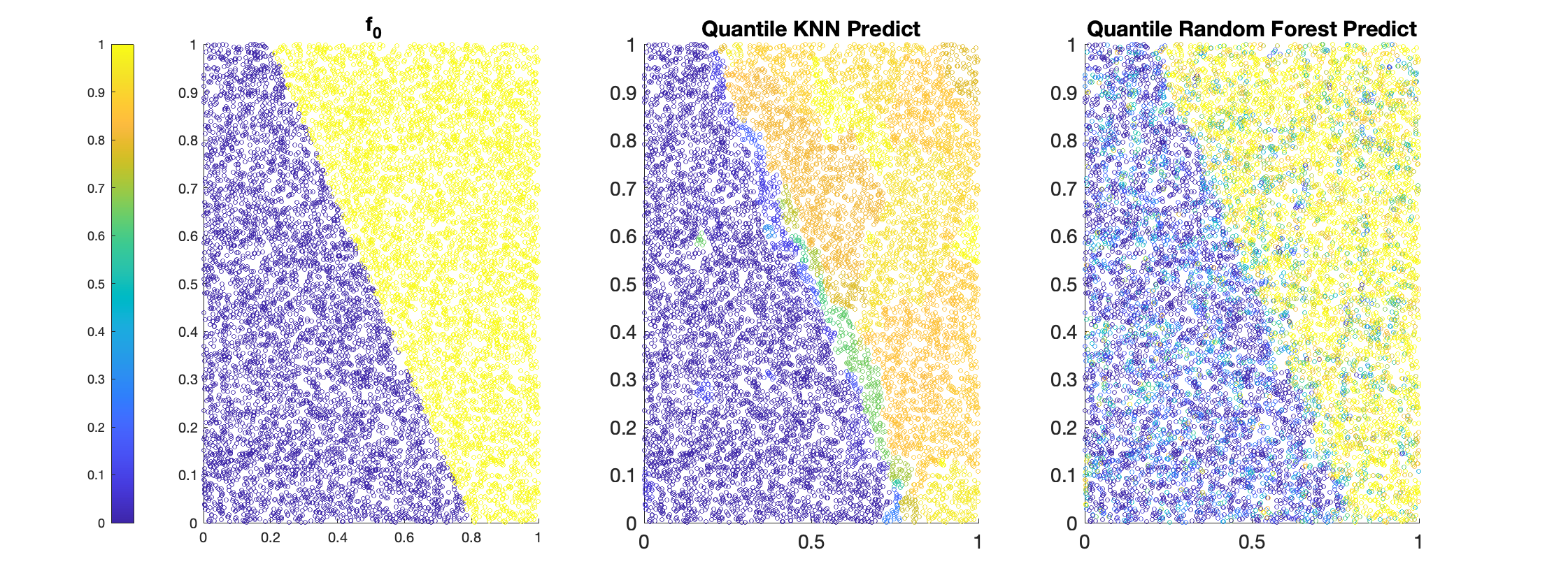
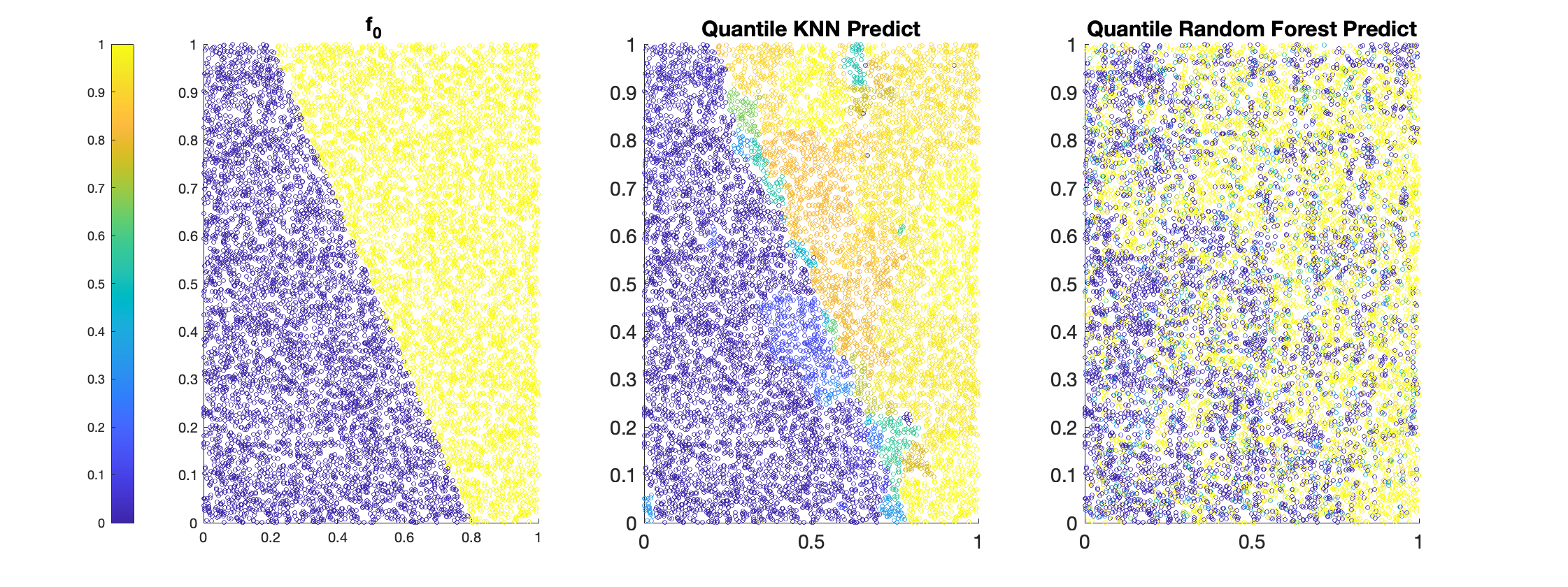
Scenario 1
We generate $x_{i}$ uniformly from $[0,1]^{2}$, and define $f_{0}:[0,1]^{2}\rightarrow\{0,1\}$ by

$$f_{0}(x)=\begin{cases}1&\text{if }\ \frac{5}{4}x_{i1}+\frac{3}{4}x_{i2}>1,\\ 0&\text{otherwise.}\end{cases}$$

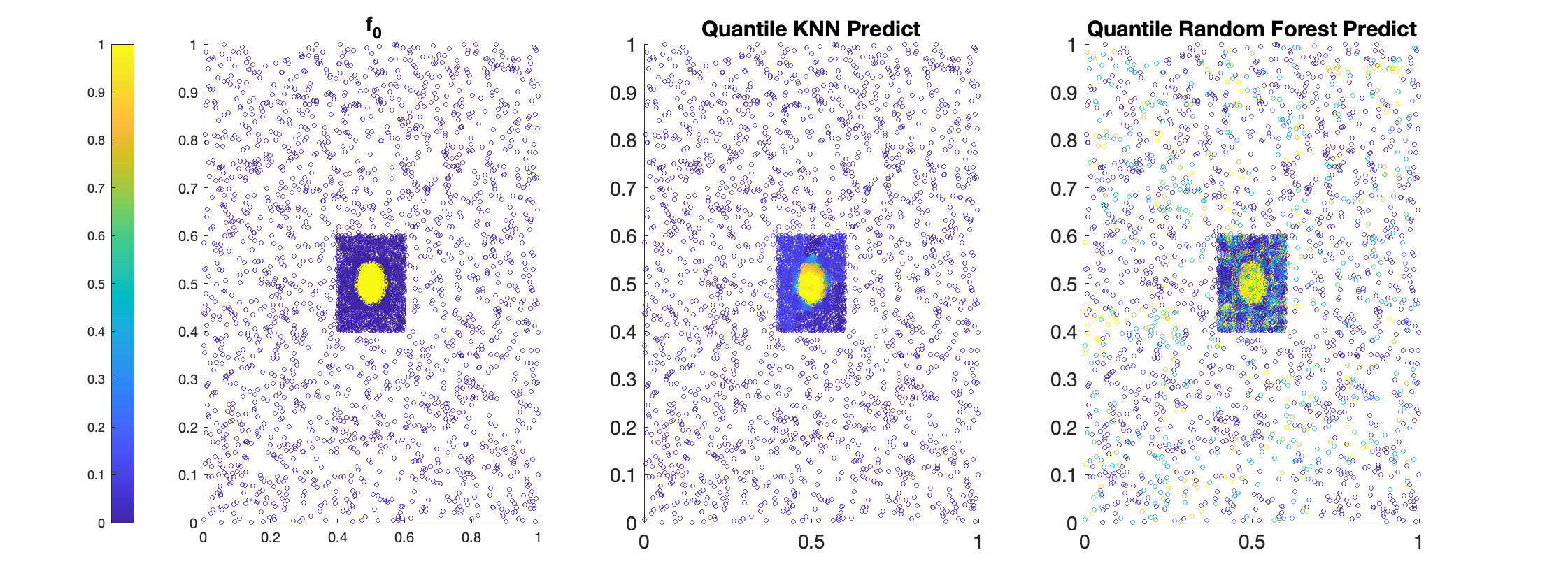
Scenario 2
In this case, we generate $X\in\mathbb{R}^{2}$ according to the probability density function

$$\begin{split}p(x)&=\frac{1}{5}\textbf{1}_{\{[0,1]^{2}\backslash[0.4,0.6]^{2}\}}(x)+\frac{16}{25}\textbf{1}_{\{[0.45,0.55]^{2}\}}(x)\\ &\ \ \ +\frac{4}{25}\textbf{1}_{\{[0.4,0.6]^{2}\backslash[0.45,0.55]^{2}\}}(x).\end{split}$$

The function $f_{0}:\ [0,1]^{2}\rightarrow\mathbb{R}$ is defined as

$$f_{0}(x)=\textbf{1}_{\{\|x-\frac{1}{2}(1,1)^{\top}\|^{2}_{2}\leq\frac{2}{1000}\}}(x).$$

Scenario 3
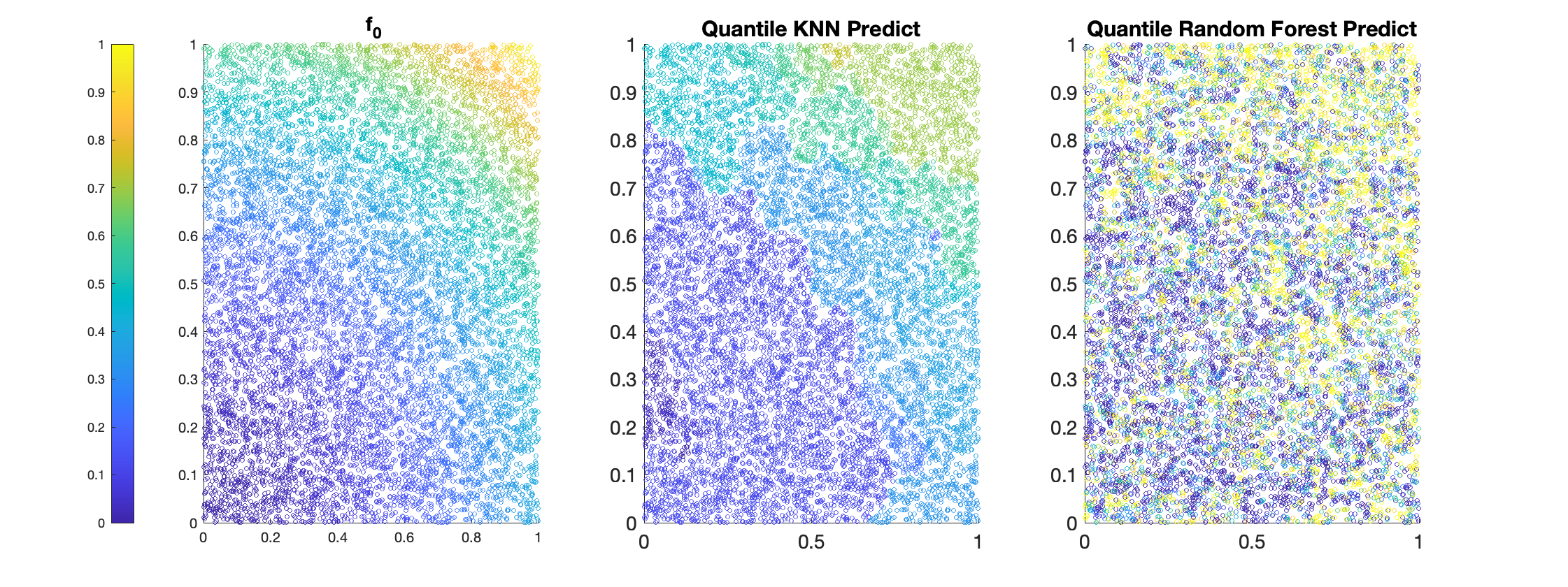
Again, $x_{i}$ are from uniform $[0,1]^{2}$. The smooth function $f_{0}:\ [0,1]^{2}\rightarrow\mathbb{R}$ is defined as

$$f_{0}(x_{i})=0.4x_{i1}^{2}+0.6x_{i2}^{2}.$$

Scenario 4
The function $f_{0}:\ [0,1]^{d}\rightarrow\mathbb{R}$ is defined as

$$f_{0}(x)=\begin{cases}1&\text{if }\ \|x-\frac{1}{4}1_{d}\|_{2}<\|x-\frac{3}{4}1_{d}\|_{2},\\ -1&\text{otherwise,}\end{cases}$$

and the density $p$ is uniform in $[0,1]^{d}$. The errors are chosen as $(x^{\top}\beta)\epsilon$, where $\beta=(\frac{1}{d},...,\frac{1}{d})^{\top}$. Here we simulate with $d=5$.

The scenarios above have been chosen to illustrate the local adaptivity of our proposed approach to discontinuities of the quantile function. Scenario 1 consists of a piecewise constant median function. Scenario 2 is borrowed from Padilla et al. (2020a) and also has a piecewise constant median. However, the covariates in Scenario 2 are not uniformly drawn and are actually highly concentrated in a small region of the domain. Scenario 3 is a smooth function, and Scenario 4 is taken from Padilla et al. (2020a). In the latter we also have a piecewise constant quantiles, but the boundaries of the different pieces are not axis aligned, and the errors are heteroscedastic.

n	Scenario	$\epsilon$	$\tau$	QKNN	QRF	KNN
100	1	N(0,1)	0.5	0.2364 (0.0628)	0.2242 (0.0467)	0.1507 (0.0365)
1000	1	N(0,1)	0.5	0.1225 (0.0117)	0.1569 (0.0116)	0.0872 (0.0239)
5000	1	N(0,1)	0.5	0.0983 (0.0024)	0.1348 (0.0047)	0.0540 (0.0022)
10000	1	N(0,1)	0.5	0.0370 (0.0019)	0.1279 (0.0028)	0.0292 (0.0010)
100	1	Cauchy(0,1)	0.5	0.1776 (0.0746)	3059.63 (54248)	35.4988 (124.19)
1000	1	Cauchy(0,1)	0.5	0.1440 (0.0817)	26640.10 (179298)	2816.1 (7691.6)
5000	1	Cauchy(0,1)	0.5	0.1326 (0.0740)	34038.86 (196566)	4628.8 (7989.0)
10000	1	Cauchy(0,1)	0.5	0.0962 (0.0642)	57748.95 (200327)	4799.0 (7249.6)
100	2	$t_{3}$	0.5	0.1838 (0.0467)	0.5591 (0.3569)	0.2374 (0.0595)
1000	2	$t_{3}$	0.5	0.0780 (0.0135)	0.3935 (0.0875)	0.1428 (0.0536)
5000	2	$t_{3}$	0.5	0.0364 (0.0050)	0.3479 (0.0477)	0.0622 (0.0165)
10000	2	$t_{3}$	0.5	0.0265 (0.0024)	0.3311 (0.0457)	0.0542 (0.0097)
100	3	$t_{2}$	0.5	0.0470 (0.0253)	1.6723 (4.8880)	0.1545 (0.4188)
1000	3	$t_{2}$	0.5	0.0174 (0.0050)	1.5363 (2.9381)	0.0510 (0.0230)
5000	3	$t_{2}$	0.5	0.0075 (0.0015)	1.4207 (2.1827)	0.0414 (0.0106)
10000	3	$t_{2}$	0.5	0.0059 (0.0019)	1.2910 (1.1924)	0.0409 (0.0102)
100	4	$t_{3}$	0.9	0.7413 (0.2180)	0.6948 (0.5340)	*
1000	4	$t_{3}$	0.9	0.3568 (0.1192)	0.5374 (0.2656)	*
5000	4	$t_{3}$	0.9	0.2889 (0.0683)	0.4420 (0.0422)	*
10000	4	$t_{3}$	0.9	0.2409 (0.0173)	0.4344 (0.0548)	*
100	4	$t_{3}$	0.1	1.1563 (0.3923)	0.8877 (0.6858)	*
1000	4	$t_{3}$	0.1	0.4160 (0.1542)	0.6224 (0.2667)	*
5000	4	$t_{3}$	0.1	0.3074 (0.0503)	0.4897 (0.0644)	*
10000	4	$t_{3}$	0.1	0.2597 (0.0301)	0.4536 (0.0494)	*

Table 1: Mean squared error $\frac{1}{n}\sum_{i=1}^{n}(\hat{\theta}_{i}-\theta_{i}^{*})^{2}$, averaging over 500 Monte Carlo simulations for the different methods, sample sizes, errors, quantiles considered. The numbers in parentheses indicate the standard Monte Carlo errors over the replications.

Figure 1 displays the true function and the estimates from both quantile $K$-NN fused lasso and quantile random forest under Scenarios 1, 2 and 3. Clearly, quantile $K$-NN fused lasso provides more reasonable estimation in all cases. Quantile random forest estimates are more noisy and the performance is even poorer under Cauchy errors.

The results presented in Table 1 indicate that overall, quantile $K$-NN fused lasso outperforms the competitors in most scenario. As expected, for estimating functions with Gaussian errors like Scenario 1, regular $K$-NN fused lasso is the best method. For Scenarios 2 and 3, when estimating the conditional median of piecewise continuous or continuous functions with heavy-tail errors (such as Cauchy and $t$-distributions), quantile $K$-NN fused lasso achieve the smallest mean square errors over the other two methods.

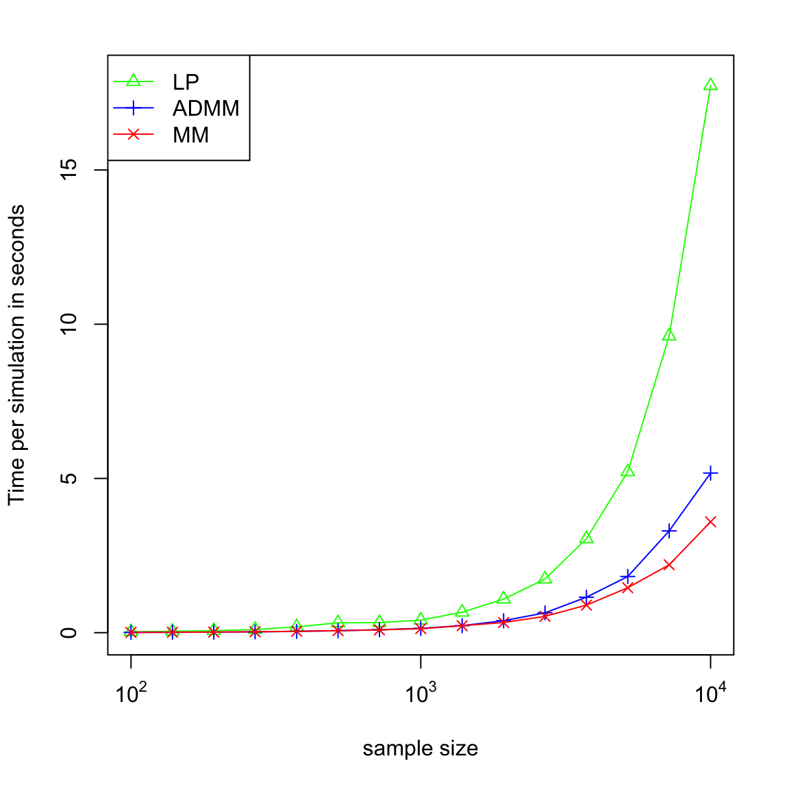
We also compare the performance of linear programming the two algorithms discussed in Section 3, with simulated data from Scenario 3. We obtain almost identical estimators from the three algorithms under the same choice of $\lambda$. Regarding computational time, we record the averaged time consumed over 100 simulations for each algorithm. Figure 2 demonstrates that majorize-minimize (MM) is the most efficient one among the three algorithms, and linear programming (LP) can be very expensive in operational time for large-size problems.

Figure 1: Comparison among observations and estimates from Scenario 1 with Gaussian errors (the first row), Scenario 1 with Cauchy errors (the second row), Scenario 2 (the third row), and Scenario 3 (the fourth row). Left column: the function $f_{0}$ evaluated at the observed $x_{i}$ for $i=1,\ldots,n$, with $n=10000$. The horizontal and vertical axis of each panel correspond to the coordinates of $x_{i}$. Middle column: the corresponding estimate of $f_{0}$ obtained via quantile $K$-NN fused lasso. Right column: the estimate of $f_{0}$ obtained via quantile random forest.

Figure 2: A log-scaled plot of time per simulation of LP, ADMM and MM algorithm against problem size $n$ (15 values from $10^{2}$ up to $10^{4}$). For each algorithm, the time to compute the estimate for one simulated data is averaged over 100 Monte Carlo simulations.

5.2 Real Data

5.2.1 California Housing Data

In this section, we conduct an experiment of predicting house value in California based on median income and average occupancy, similar to the experiment in Petersen et al. (2016). The data set, consisting of 20,640 measurements, was originally used in Pace and Barry (1997) is publicly available from the Carnegie Mellon StatLib data repository (lib.stat.cmu.edu).

Figure 3: Comparison between predictions from two methods for California housing data, with respect to $\tau=0.1,0.5,0.9$. The plot at the top presents the true testing data value, and the color scale is the same among all plots.

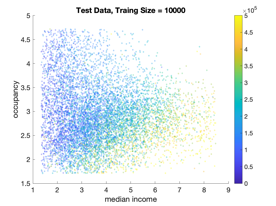
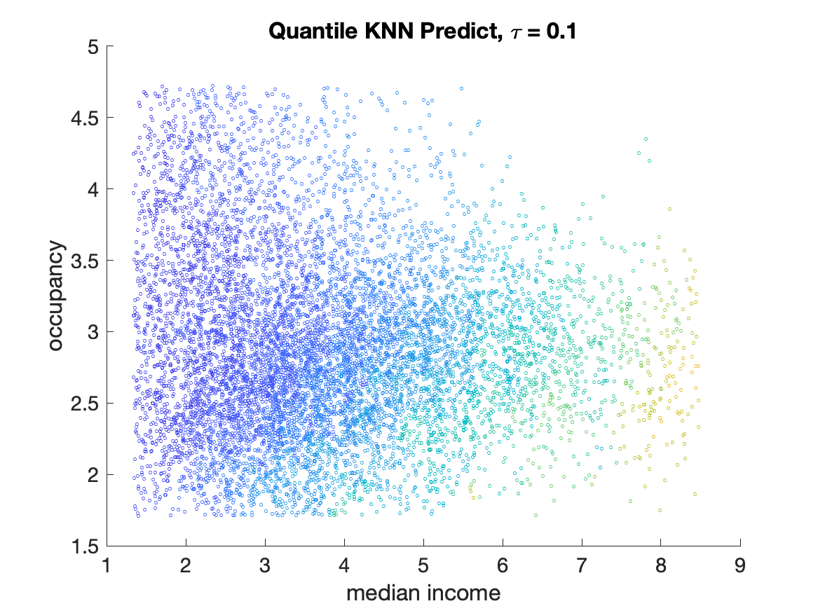
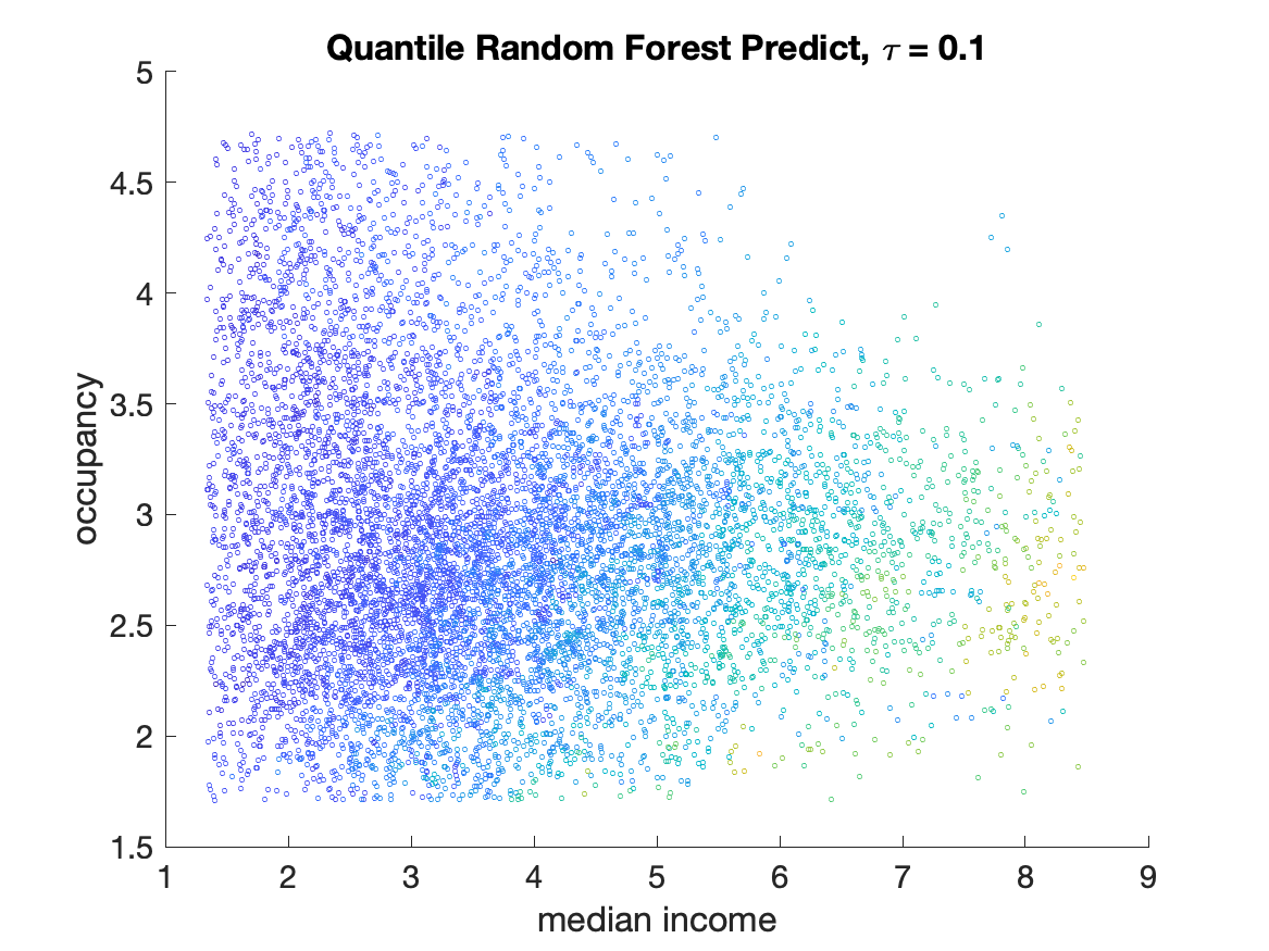
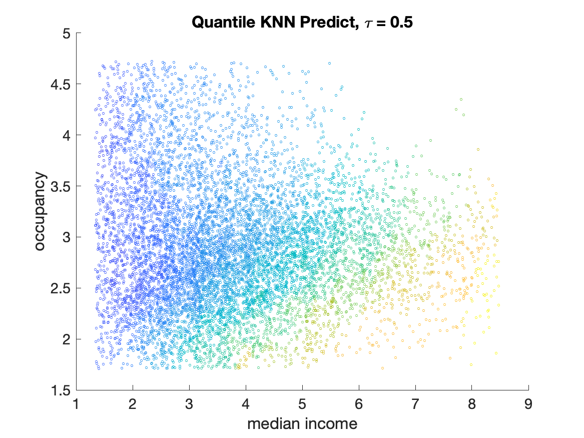
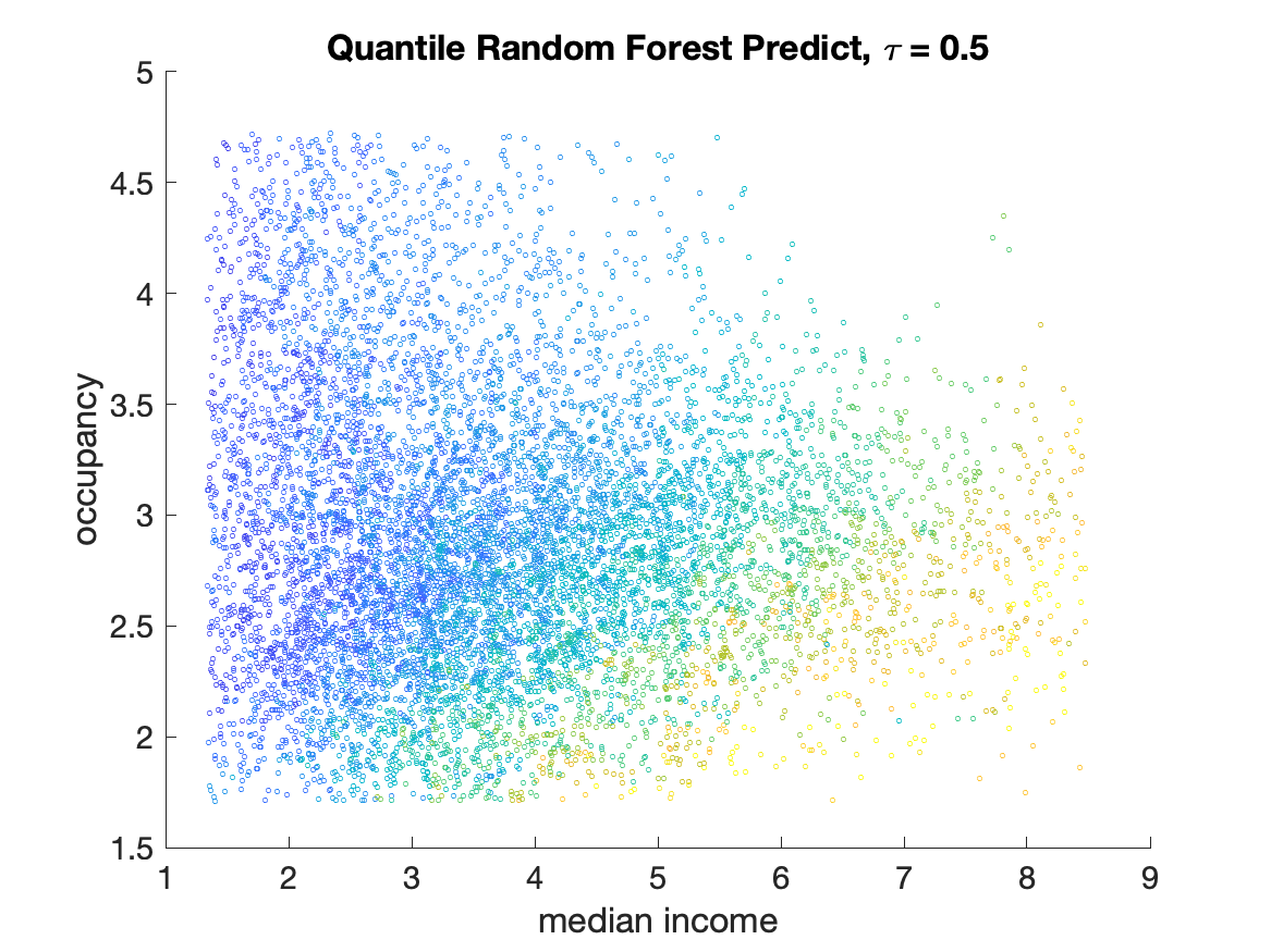
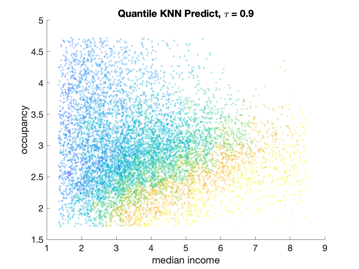
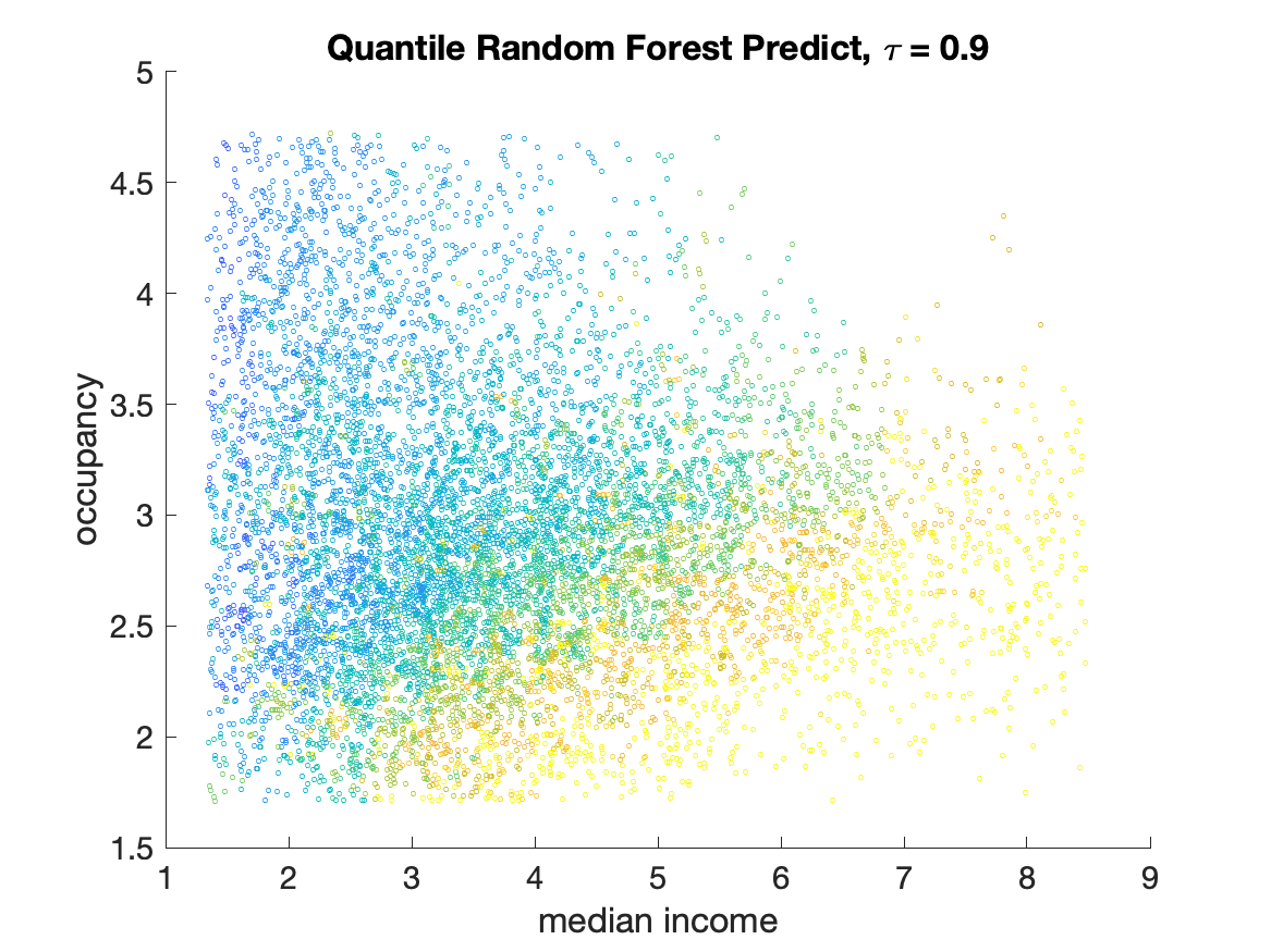
We perform 100 train-test random splits the data, with training sizes 1000, 5000, and 10000. For each split the data not in the training set is treated as testing data. For median estimation, we compare averaged mean squared prediction errors of the test sets (after taking the log of housing price) from quantile $K$-NN fused lasso and quantile random forest; besides, we construct 90$\%$ and 95$\%$ prediction intervals from both methods and report the proportion of true observations in the test set that fall in the intervals. Both evaluations are averaged over 100 repetitions for each method. The tuning parameter $\lambda$ for quantile $K$-NN fused lasso is chosen based on the BIC criteria for each training and the parameters for quantile random forest are selected as default.

From the results in Table 2, quantile $K$-NN fused lasso has better performance than quantile random forest in all cases. The result agrees with the nature of piecewise continuity in housing price, that guarantee the advantage of our proposed method over the competitor. When we illustrate the predicted values on a test set from a experiment with training size of 10,000 visually in Figure 3, we also observe a piecewise continuous structure in quantile $K$-NN fused lasso estimates, while estimates from quantile random forest contain more noise, especially for lower and higher quantiles.

Training Size	$\tau$	QKNN	QRF
1000	0.5	0.1553 (0.0032)	0.1679 (0.0026)
5000	0.5	0.1485 (0.0016)	0.1646 (0.0016)
10000	0.5	0.1479 (0.0017)	0.1623 (0.0019)
Training Size	$\tau$	QKNN	QRF
1000	0.9	0.8405 (0.0141)	0.8315 (0.0086)
5000	0.9	0.8569 (0.0076)	0.8334 (0.0040)
10000	0.9	0.8585 (0.0061)	0.8337 (0.0041)
1000	0.95	0.9163 (0.0127)	0.8887 (0.0084)
5000	0.95	0.9216 (0.0099)	0.8891 (0.0040)
10000	0.95	0.9274 (0.0097)	0.8902 (0.0042)

Table 2: Average test set prediction error (across the 100 test sets) on California housing data. For median, we report the mean squared errors; for other quantiles ($\tau\in\{0.9,0.95\}$), we report the averaged proportion of the true data located in the predicted confidence interval. Standard Monte Carlo errors are recorded in parentheses. The number of nearest neighbors, $K$ is chosen as 5 for quantile $K$-NN fused lasso.

Finally, it is clear from Table 2 that both quantile $K$-NN fused lasso and quantile random forest have coverage probabilities are noticeably lower than the true nominal level. Since the results in Table 2 correspond to a real data set, training on a subset and predicting on a different subset of the data, we are not aware of how to improve the coverage for both of the competing methods.

5.2.2 Chicago Crime Data

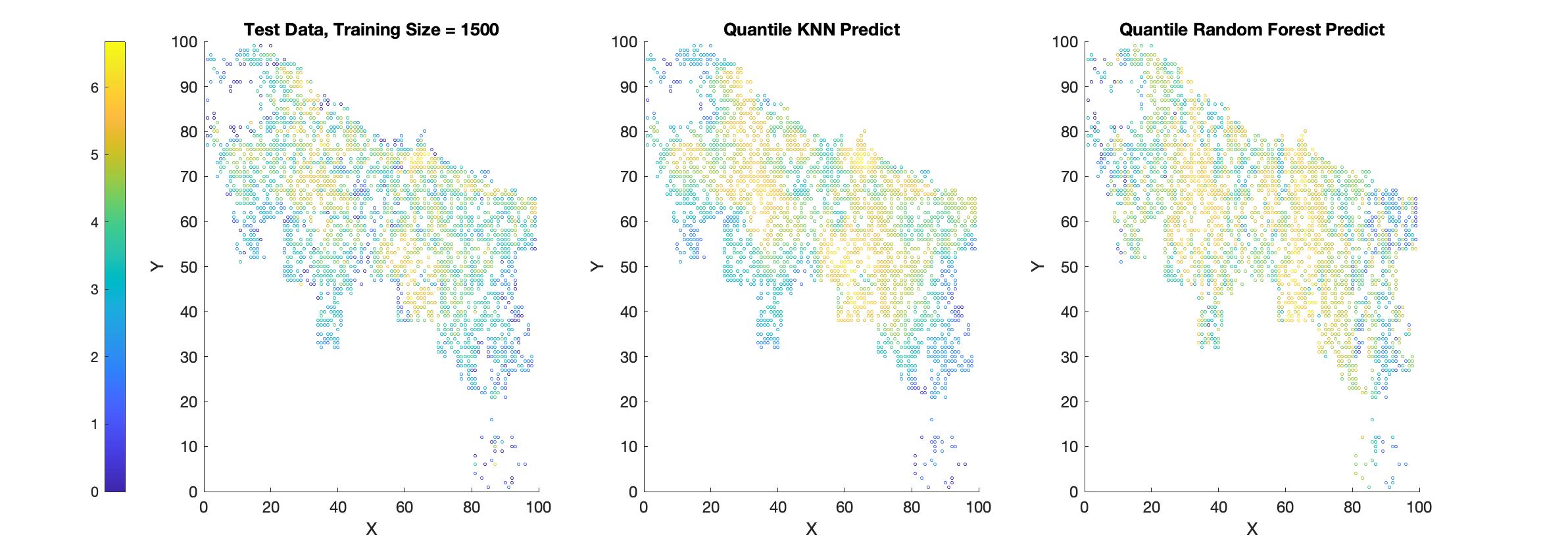
We apply quantile $K$-NN fused lasso and quantile random forest to a dataset of publicly-available crime report counts in Chicago, Illinois in 2015. We preprocess the dataset in the same way as Tansey et al. (2018) by merging all observations into a fine-grained 100 $\times$ 100 grid based on latitude and longitude, taking the log of the total counts in each cell, and omitting all cells with zero count. The resulting preprocessed data contains a total number of 3756 data points along the grid. Similar to the experiment on California housing data, we perform a train-test split with training size 500, 1000, 1500, and 2000, and model on the median counts according to the position on the $X$ and $Y$ axes of the grid. We then predict the value on test set and report the averaged square errors over 100 test sets. The parameters for both methods are selected in the same way as in the previous experiment.

Training Size	$\tau$	QKNN	QRF
500	0.5	1.2161 (0.0441)	1.1441 (0.0479)
1000	0.5	1.0151 (0.0374)	0.9836 (0.0417)
1500	0.5	0.9138 (0.0343)	0.8959 (0.0380)
2000	0.5	0.8476 (0.0409)	0.8383 (0.0417)

Table 3: Average test set prediction errors (across the 100 test sets) with standard errors on Chicago Crime data.

From the results of Table 3, we see that quantile $K$-NN fused lasso still outperforms quantile random forest in MSE if the training size is at least 1500. We notice that for small sample size, our method suffers. This is presumably due to the fact that the raw data is not smooth enough. Yet, Figure 4 shows that quantile $K$-NN fused lasso capture local patterns more successfully than quantile random forest in most regions.

Figure 4: Left: one test data from Chicago Crime Data, under training size 1500. Middle: the estimate obtained via quantile $K$-NN fused lasso. Right: the estimate obtained via quantile random forest.

6 Conclusion

In this paper we have proposed and studied a method for estimating of quantile functions that are piecewise constant. Such classes of functions naturally arise in real-life data. Estimating accurately signals with such structure is an important but challenging research topic arising in many practical contexts. However, there is a lack of existing literature on robust estimation of piecewise constant or piecewise Lipschitz signals in multivariate settings. Motivated by this, we have proposed the quantile $K$-NN fused lasso estimator.

Our numerical experiments on different real-life and simulated examples lay out empirical evidence of the superior robustness and local adaptivity of our estimator over other state-of-the-art methods. We have presented two algorithms to efficiently compute the solutions to the corresponding optimization problem behind our method. Our theoretical analysis extends previous work on $K$-NN fused lasso (Padilla et al., 2020a) and quantile trend filtering (Padilla and Chatterjee, 2020). Specifically, we have shown that the quantile $K$-NN fused lasso estimator achieves an optimal convergence rate of $n^{-1/d}$ for estimating a $d$-dimensional piecewise Lipschitz quantile function. This result is guaranteed under mild assumptions on data, and thus our estimator can be applied to more general models rather than only those with sub-Gaussian errors.

Appendix A. Closed-form Solution to the Primal in ADMM Algorithm

In Section 3.1, we introduce an ADMM algorithm to compute quantile $K$-NN estimates. The algorithm requires to solve the primal problem (13)

$$\ \ \ \ \theta\leftarrow\underset{\theta\in\mathbb{R}^{n}}{\arg\min}\ \left\{\sum_{i=1}^{n}\rho_{\tau}(y_{i}-\theta_{i})+\frac{R}{2}\|\theta-z+u\|^{2}\right\}.$$

We can solve the problem coordinate-wisely: for $i=1,...,n$, we find the minimizer

$$\ \ \ \ \theta_{i}\leftarrow\underset{\theta_{i}\in\mathbb{R}}{\arg\min}\ \left\{\rho_{\tau}(y_{i}-\theta_{i})+\frac{R}{2}(\theta_{i}-z_{i}+u_{i})^{2}\right\}.$$

By definition,

$$\rho_{\tau}(y_{i}-\theta_{i})=\begin{cases}\tau(y_{i}-\theta_{i})&\text{ if }\ y_{i}-\theta_{i}>0,\\ (\tau-1)(y_{i}-\theta_{i})&\text{ if }\ y_{i}-\theta_{i}<0,\\ 0&\text{ if }\ y_{i}-\theta_{i}=0.\end{cases}$$

We discuss the three cases separately.

(1) When $y_{i}-\theta_{i}>0$, $\theta_{i}\leftarrow\arg\min\left\{\tau(y_{i}-\theta_{i})+\frac{R}{2}(\theta_{i}-z_{i}+u_{i})^{2}\right\}$. Take the derivative and set to 0 to obtain $\theta_{i}=z_{i}-u_{i}+\tau/R$. The condition $y_{i}-\theta_{i}>0$ then becomes $y_{i}-z_{i}+u_{i}>\tau/R$.

(2) When $y_{i}-\theta_{i}<0$, $\theta_{i}\leftarrow\arg\min\left\{(\tau-1)(y_{i}-\theta_{i})+\frac{R}{2}(\theta_{i}-z_{i}+u_{i})^{2}\right\}$. Take the derivative and set to 0 to obtain $\theta_{i}=z_{i}-u_{i}+(\tau-1)/R$. The condition $y_{i}-\theta_{i}<0$ then becomes $y_{i}-z_{i}+u_{i}<(\tau-1)/R$.

(3) When $y_{i}-\theta_{i}=0$, it is simple to get $\theta_{i}=y_{i}$.

To summarize, the closed-form solution to the primal (13) is

$$\theta_{i}=\begin{cases}z_{i}-u_{i}+\frac{\tau}{R}&\text{ if }y_{i}-z_{i}+u_{i}>\frac{\tau}{R},\\ z_{i}-u_{i}+\frac{\tau-1}{R}&\text{ if }y_{i}-z_{i}+u_{i}<\frac{\tau-1}{R},\\ y_{i}&\text{ otherwise; }\end{cases}$$

for $i=1,...,n$.

Appendix B. Sensitivity of Initialization in the ADMM Algorithm

In this section, we examine how the convergence of Algorithm 1 is sensitive to different initials. Recall that Algorithm 1 requires an initialization of $\theta^{(0)}$, $z^{(0)}$ and $u^{(0)}$. A practical way to choose these initials is to set $\theta^{(0)}=z^{(0)}=y,u^{(0)}=0$, where $y$ is the input data, as defined in Algorithm 1. Here, we try three other initializations to assess the sensitivity to the initials:

(1) The setup in Algorithm 1: $\theta^{(0)}=z^{(0)}=y,u^{(0)}=0$.

(2) We add perturbations to the first setup: $\theta^{(0)}=y+v_{1},z^{(0)}=y+v_{2},u^{(0)}=v_{3}$, where $v_{1},v_{2},v_{3}\overset{\text{ind}}{\sim}N(0,I_{n})$.

(3) Random initialization: $\theta^{(0)}=w_{1},z^{(0)}=w_{2},u^{(0)}=w_{3}$, where $w_{1},w_{2},w_{3}\overset{\text{ind}}{\sim}N(0,I_{n})$.

(4) Random initialization with a large multiplication factor: $\theta^{(0)}=50s_{1},z^{(0)}=50s_{2},u^{(0)}=50s_{3}$, where $s_{1},s_{2},s_{3}\overset{\text{ind}}{\sim}N(0,I_{n})$.

We use the data generation mechanism in Scenario 2 from the main content, and errors are independently drawn from a $t$-distribution with 3 degrees of freedom. The regularization parameter $\lambda$ is set to be fixed as 0.5. We replicate the simulation 500 times with a sample size $n=10000$. Note that the input data and perturbations are generated independently in every replication. For each initialization setup, we record the averaged value of the objective function $\sum_{i=1}^{n}\rho_{\tau}(y_{i}-\theta_{i})+\lambda\|\nabla_{G}\theta\|_{1}$ after each iteration and the number of iterations to converge when we set $\kappa=0.01$ in Step 3 of Algorithm 1.

Figure 5: Averaged value of objective function (over 500 replications) after each iteration step for different initializations.

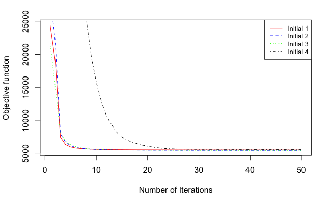
From Figure 5, we observe that the value of the objective function converges very fast to the optimal minimum within only tens of iterations, regardless of the random initialization that is used. If we look at the number of iterations shown in Table 4, the first three initializations have relatively the same convergence speed. If there exists a large deviation between the initial value and the true signal like in the last setup, the ADMM algorithm takes slightly longer time to converge. Overall, the ADMM algorithm is insensitive to random initialization and fast convergence is observed in practice.

Initialization	Averaged number of iterations to converge
(1)	11
(2)	11.13
(3)	11
(4)	26.65

Table 4: Number of iterations to converge under different initializations, averaging over 500 Monte Carlo simulations.

Appendix C. General Lemmas

The following lemmas hold by conditioning on $\{x_{i}\}_{i=1}^{n}$.

Definition 9

The function $\Delta^{2}$ is defined as

$$\Delta^{2}(\delta):=\sum_{i=1}^{n}\min\{|\delta_{i}|,\delta_{i}^{2}\},$$

where $\delta_{i}\in\mathbb{R}^{n}$. We also write $\Delta(\delta)=\{\Delta^{2}(\delta)\}^{1/2}$.

Definition 10

For a set $S\subset\mathbb{R}^{n}$, the sub-Gaussian width of $S$ is defined as

$$SGW(S)=\mathbb{E}\left(\sup_{v\in S}\sum_{i=1}^{n}s_{i}v_{i}\right),$$

where $s_{1},...,s_{n}$ are independent 1-subgaussian random variables.

The notation of sub-Gaussian width is not used very often in literature compared to a similar definition of Gaussian width,

$$GW(S)=\mathbb{E}\left(\sup_{v\in K}\sum_{i=1}^{n}z_{i}v_{i}\right),$$

where $z_{1},...,z_{n}$ are independent standard normal random variables. In fact, the sub-Gaussian width shares many common properties with the Gaussian width, as we can upper bound the sub-Gaussian width by a constant times the Gaussian width using generic chaining; see Chapter 4 in Talagrand (2005) and also Banerjee et al. (2014) for precise explanations.

Definition 11

We define the empirical loss function

$$\hat{M}(\theta)=\sum_{i=1}^{n}\hat{M}_{i}(\theta_{i}),$$

where

$$\hat{M}_{i}(\theta_{i})=\rho_{\tau}(y_{i}-\theta_{i})-\rho_{\tau}(y_{i}-\theta^{*}_{i}).$$

Setting $M_{i}(\theta_{i})=\mathbb{E}(\rho_{\tau}(y_{i}-\theta_{i})-\rho_{\tau}(y_{i}-\theta^{*}_{i}))$, the population version of $\hat{M}$ becomes

$$M(\theta)=\sum_{i=1}^{n}M_{i}(\theta_{i}).$$

Now, we consider the $M$-estimator

$$\begin{split}\hat{\theta}\ \ =\ \ &\underset{\theta\in\mathbb{R}^{n}}{\arg\min}\ \ \ \ \ \hat{M}(\theta)\\ &\text{subject to}\ \ \theta\in S,\end{split}$$ (20)

and $\theta^{*}\in\arg\min_{\theta\in\mathbb{R}^{n}}M(\theta)$. Throughout, we assume that $\theta^{*}\in S\subset\mathbb{R}^{n}$.

Lemma 12

With the notation from before,

$$M(\hat{\theta})\leq\sup_{v\in S}\left\{M(v)-\hat{M}(v)\right\}.$$

Proof. See the proof of Lemma 10 in Padilla and Chatterjee (2020).

Lemma 13

Suppose that Assumption 2 holds. Then there exists a constant $c_{\tau}>0$ such that for all $\delta\in\mathbb{R}^{n}$, we have

$$M(\theta+\delta)\geq c_{\tau}\Delta^{2}(\delta).$$

Proof. See the proof of Lemma 14 in Padilla and Chatterjee (2020).

Corollary 14

Under Assumption 2, if $\theta^{*}\in S$, we have that

$$\mathbb{E}\left\{\Delta^{2}(\hat{\theta}-\theta^{*})\right\}\leq\mathbb{E}\left[\sup_{v\in S}\left\{M(v)-\hat{M}(v)\right\}\right].$$ (21)

Next, we proceed to bound the right hand side of (21).

Lemma 15

(Symmetrization) Under Assumption 2, we have that

$$\mathbb{E}\left[\sup_{v\in S}\left\{M(v)-\hat{M}(v)\right\}\right]\leq 2\mathbb{E}\left\{\sup_{v\in S}\sum_{i=1}^{n}\xi_{i}\hat{M}_{i}(v_{i})\right\},$$

where $\xi_{1},...,\xi_{n}$ are independent Rademacher variables independent of $y_{1},...,y_{n}$.

Proof. See the proof of Lemma 11 in Padilla and Chatterjee (2020).

Lemma 16

(Contraction principle) Under Assumption 2, we have that

$$\mathbb{E}\left\{\sup_{v\in S}\sum_{i=1}^{n}s_{i}\hat{M}_{i}(v_{i})\right\}\leq 2SGW(S-\theta^{*})=2SGW(S),$$

where $s_{1},...,s_{n}$ are independent 1-subgaussian random variables independent of $y_{1},...,y_{n}$.

Proof. Recall that $\hat{M}_{i}(v_{i})=\rho_{\tau}(y_{i}-v_{i})-\rho_{\tau}(y_{i}-\theta^{*}_{i})$. Clearly, these are 1-Lipschitz continuous functions. Therefore,

$$\mathbb{E}\left\{\sup_{v\in S}\sum_{i=1}^{n}s_{i}\hat{M}_{i}(v_{i})\right\} =\mathbb{E}\left(\mathbb{E}\left\{\sup_{v\in S}\sum_{i=1}^{n}s_{i}\hat{M}_{i}(v_{i})\bigg{|}y\right\}\right)$$

$$\leq\mathbb{E}\left(\mathbb{E}\left\{\sup_{v\in S}\sum_{i=1}^{n}s_{i}v_{i}\bigg{|}y\right\}\right)$$

$$=\mathbb{E}\left\{\sup_{v\in S}\sum_{i=1}^{n}s_{i}(v_{i}-\theta^{*})\right\}+\mathbb{E}\left(\sum_{i=1}^{n}s_{i}\theta^{*}\right)$$

$$=\mathbb{E}\left\{\sup_{v\in S}\sum_{i=1}^{n}s_{i}(v_{i}-\theta^{*})\right\}$$

where the inequality follows from the Gaussian version of Talagrand’s contraction principle, see corallary 3.17 in Ledoux and Talagrand (2013) and 7.2.13 in Vershynin (2018). $\hfill{\square}$

Appendix D. $K$-NN Embeddings

This section follows from Section D and E in Padilla et al. (2020a) and it originally appeared in the flow-based proof of Theorem 4 in Von Luxburg et al. (2014). The main idea is to embed a mesh on a $K$-NN graph corresponding to the given observations $X=(x_{1},...,x_{n})$ under Assumptions 3-5 so that we are able to bound the total variation along the grid graph from below. In this way, we can further derive an upper bound on the loss of the optimization problem (8) and (10) with respect to the loss function defined in Definition 9.

First, we need to construct a valid grid discussed in Definition 17 of Von Luxburg et al. (2014) with a minor modification. With high probability, a valid grid graph $G$ satisfies the following: (i) the grid width is not too small: each cell of the grid contains at least one of the design points; (ii) the grid width is not too large: points in the same or neighboring cells of the grid are always connected in the $K$-NN graph.

Given $N\in\mathbb{N}$, a $d$-dimensional grid graph $G_{\text{lat}}\in[0,1]^{d}$ has vertex set $V_{\text{lat}}$ and edge set $E_{\text{lat}}$. The grid graph has equal side lengths, and the total number of nodes $|V_{\text{lat}}|=N^{d}$. Without loss of generality, we assume that the nodes of the grid correspond to the points

$$P_{\text{lat}}(N)=\left\{\left(\frac{i_{1}}{N}-\frac{1}{2N},...,\frac{i_{d}}{N}-\frac{1}{2N}\right):i_{1},...,i_{d}\in\{1,...,N\}\right\}.$$ (22)

Moreover, for $z,z^{\prime}\in P_{\text{lat}}(N)$, $(z,z^{\prime})\in E_{\text{lat}}(N)$ if and only if $\|z-z^{\prime}\|_{2}=\frac{1}{N}$.

Now, we define $I(N)=h^{-1}\{P_{\text{lat}}(N)\}$ as the mesh in the covariate space $\mathcal{X}$ corresponding to the grid graph $G_{\text{lat}}(N)\in[0,1]^{d}$ through the homeomorphism $h$ from Assumption 5. In general, $I(N)$ performs as a quantifization in the domain $\mathcal{X}$; see Alamgir et al. (2014) for more details. We denote the elements in $I(N)$ by $u_{1},...,u_{N^{d}}$, and define a collection of cells $\{C(x)\}\in\mathcal{X}$ for $x\in I(N)$ as

$$C(x)=h^{-1}\left(\left\{z\in[0,1]^{d}:h(x)=\underset{x^{\prime}\in P_{\text{lat}}(N)}{\arg\min}\ \|z-x^{\prime}\|_{\infty}\right\}\right).$$ (23)

In order to analyze the behavior of the proposed estimator $\hat{\theta}$ through the grid embedding, we construct two vectors denoted by $\theta_{I}\in\mathbb{R}^{n}$ and $\theta^{I}\in\mathbb{R}^{N^{d}}$ for any signal $\theta\in\mathbb{R}^{n}$.

The first vector, $\theta_{I}\in\mathbb{R}^{n}$ incorporates information about the samples $X=(x_{1},...,x_{n})$ and the cells $\{C(x)\}$. The idea is to force covariates $x_{i}$ fallen in the same cell to take the same signal value after mapping with the homeomorphism. Formally, we define

$$(\theta_{I})_{i}=\theta_{j}\ \ \ \ \text{where }\ j=\underset{l=1,...,n}{\arg\min}\ \|h(P_{I}(x_{i}))-h(x_{l})\|_{\infty},$$ (24)

where $P_{I}(x)$ is the point in $I(N)$ such that $x\in C(P_{I}(x))$ and if there exists multiple points satisfying the condition, we arbitrarily select one.

The second vector, $\theta^{I}\in\mathbb{R}^{N^{d}}$ records coordinates corresponding to the different nodes of the mesh (centers of cells), and is associated with $\theta_{I}$. We first induce a signal in $\mathbb{R}^{N^{d}}$ corresponding to the elements in $I(N)$ as

$$I_{j}=\{i=1,...,n:P_{I}(x_{i})=u_{j}\},\ \text{for }j=1,...,N^{d}.$$

If $I_{j}\neq\emptyset$, then there exists $i_{j}\in I_{j}$ such that $(\theta_{I})_{i}=\theta_{i_{j}}$ for all $i\in I_{j}$; if $I_{j}$ is empty, we require $\theta_{i_{j}}=0$. We can thus define

$$\theta^{I}=\left(\theta_{i_{1}},...,\theta_{i_{N^{d}}}\right).$$

Note that in the proof of Lemma 11 in Padilla et al. (2020a), the authors showed that under Assumptions 3-5, with probability approaching 1,

$$\max_{x\in I(N)}|C(x)|\leq\textup{poly}(\log n).$$ (25)

We will use this inequality in our proofs later, but we will not make the polynomial function of $\log n$ explicit.

Appendix E. Definition of Piecewise Lipschitz

To make sure Assumption 1 is valid, we require a piecewise Lipschitz condition on the regression function $f_{0}$. In this section, we provide the detailed definition of the class of piecewise Lipschitz functions, followed from Definition 1 in Padilla et al. (2020a). All notations follow the same from the main context, besides an extra notation on the boundary of a set $A$, denoted by $\partial A$.

Definition 17

Let $\Omega_{\epsilon}:=[0,1]^{d}\backslash B_{\epsilon}(\partial[0,1]^{d})$. We say that a bounded function $g:[0,1]^{d}\rightarrow\mathbb{R}$ is piecewise Lipschitz if there exists a set $\mathcal{S}\subset(0,1)^{d}$ that has the following properties:

• The set $\mathcal{S}$ has Lebesgue measure zero.

• For some constants $C_{\mathcal{S}},\epsilon_{0}>0$, we have that $\mu(h^{-1}\{B_{\epsilon}(\mathcal{S})\cap([0,1]^{d}\backslash\Omega_{\epsilon})\})\leq C_{\mathcal{S}}\epsilon$ for all $0<\epsilon<\epsilon_{0}$.

• There exists a positive constant $L_{0}$ such that if $z$ and $z^{\prime}$ belong to the same connected component of $\Omega_{\epsilon}\backslash B_{\epsilon}(\mathcal{S})$, then $|g(z)-g(z^{\prime})|\leq L_{0}\|z-z^{\prime}\|_{2}$.

Roughly speaking, a bounded function $g$ is piecewise Lipschitz if there exists a small set $\mathcal{S}$ that partitions $[0,1]^{d}$ in such a way that $g$ is Lipschitz within each connected component of the partition. Theorem 2.2.1 in Ziemer (2012) implies that if $g$ is piecewise Lipschitz, then $g$ has bounded variation on any open set within a connected component.

Appendix F. Theorem 6

F.1   Notations

For a matrix $D$, we denote its kernel by $\text{Ker}(D)$ and its Moore–Penrose inverse by $D^{\dagger}$. We also write $\Pi$ as the projection matrix onto $\text{Ker}(D)$, and denote $\text{Ker}(D)^{\perp}$ as the orthogonal complement to the kernel space of $D$.

Our goal is to upper bound the expectation of $M(\cdot)-\hat{M}(\cdot)$ in the constrained set $S$ defined by

$$S=\left\{\theta\in\mathbb{R}^{n}\ :\ \|\nabla_{G}\theta\|_{1}\leq Vn^{1-1/d}\textup{poly}(\log n)\right\},$$ (26)

where $V=\|\nabla_{G}\theta^{*}\|_{1}/[n^{1-1/d}\textup{poly}(\log n)]$ and $V\geq V^{*}$. Through the $K$-NN embedding, we can instead bound the expected loss in the embedded set defined by

$$\tilde{S}=\left\{\theta\in\mathbb{R}^{n}\ :\ \|D\theta^{I}\|_{1}\leq Vn^{1-1/d}\textup{poly}(\log n)\right\},$$ (27)

where $\theta^{I}$ follows the definition in Appendix D.

F.2   Auxiliary lemmas for Proof of Theorem 6

Lemma 18

For $v\in\mathbb{R}^{n}$, if $\|\nabla_{G}v\|_{1}\leq\tilde{V}$, and $\Delta^{2}(v-\theta^{*})\leq t^{2}$, then $\|Dv^{I}\|_{1}\leq\tilde{V}$, and $\Delta^{2}(v^{I}-\theta^{*,I})\leq c_{1}t^{2}$ for some constant $c_{1}$.

Proof. Lemma 4 in Padilla et al. (2020a) obtains the inequality

$$\|Dv^{I}\|_{1}\leq\|\nabla_{G}v\|_{1},\ \forall v\in\mathbb{R}^{.}$$

Hence, the first claim follows.

Next, we observe that for any vector $u\in\mathbb{R}^{n}$,

$$\Delta^{2}(u^{I})=\left(\sum_{j=1}^{N^{d}}\min\left\{|u_{i_{j}}|,u_{i_{j}}^{2}\right\}\right)\leq\left(\sum_{i=1}^{n}\min\left\{|u_{i}|,u_{i}^{2}\right\}\right)\leq\Delta^{2}(u),$$

for some positive constant $c_{1}$. The second claim follows then. $\hfill\square$

Lemma 18 gives us the fact that

$$\left\{v\in S:\Delta^{2}(v-\theta^{*})\leq t^{2}\right\}\subseteq\left\{v\in\tilde{S}:\Delta^{2}(v^{I}-\theta^{*,I})\leq c_{1}t^{2}\right\}.$$ (28)

Lemma 19

Under Assumptions 1-5, we have that

$$\begin{array}[]{lll}\displaystyle\mathbb{E}\left[\sup_{v\in\tilde{S}:\Delta^{2}(v^{I}-\theta^{*,I})\leq t^{2}}\sum_{i=1}^{n}\xi_{i}(v_{i}-\theta_{i}^{*})\right]&\leq&\displaystyle\textup{poly}(\log n)\mathbb{E}\left[\sup_{v\in\tilde{S}:\Delta^{2}(v^{I}-\theta^{*,I})\leq t^{2}}\sum_{j=1}^{N^{d}}\tilde{\xi}_{j}(v^{I}_{j}-\theta^{*,I}_{j})\right]\\ &&\displaystyle+2Vn^{1-1/d}\textup{poly}(\log n),\end{array}$$

where $\tilde{\xi}\in\mathbb{R}^{N^{d}}$ is a 1-subgaussian vector whose coordinates are independent.

Proof. We notice that

$$\xi^{\top}(v-\theta^{*}) =\xi^{\top}(v-v_{I})+\xi^{\top}(v_{I}-\theta_{I}^{*})+\xi^{\top}(\theta_{I}^{*}-\theta^{*})$$

$$\leq 2\|\xi\|_{\infty}\left(\|\nabla_{G}v\|_{1}+\|\nabla_{G}\theta^{*}\|_{1}\right)+\xi^{\top}(v_{I}-\theta_{I}^{*}),$$

where the second inequality holds by Lemma 4 in Padilla et al. (2020a). Moreover,

$$\xi^{\top}(v_{I}-\theta_{I}^{*})=\sum_{j=1}^{N^{d}}\sum_{l\in I_{j}}\xi_{l}(v_{i_{j}}-\theta^{*}_{i_{j}})=\left\{\max_{u\in I}|C(u)|\right\}^{1/2}\tilde{\xi}^{\top}(v^{I}-\theta^{*,I})$$

where

$$\tilde{\xi}_{j}=\left\{\max_{u\in I}|C(u)|\right\}^{-1/2}\sum_{l\in I_{j}}\xi_{l}.$$

Clearly, the $\tilde{\xi}_{1},...,\tilde{\xi}_{N^{d}}$ are independent and also 1-subgaussian as the original Rademacher random variables $\xi_{1},...,\xi_{n}$. Then, following from (25), we have

$$\xi^{\top}(v_{I}-\theta_{I}^{*})\leq\textup{poly}(\log n)\tilde{\xi}^{\top}(v^{I}-\theta^{*,I}).$$

Hence, the desired inequality holds. $\hfill\square$

Lemma 20

Let $\delta\in\mathbb{R}^{N^{d}}$ with $\Delta^{2}(\delta)\leq t^{2}$. Then

$$\|\Pi\delta\|_{\infty}\leq\frac{t^{2}}{N^{d}}+\frac{t}{\sqrt{N^{d}}}.$$

Proof. Notice that $\text{Ker}(D)=\text{span}(1_{N^{d}})$, then $\Pi\delta=\delta^{\top}v\cdot v,$ where $v=\frac{1}{\sqrt{N^{d}}}1_{N^{d}}$. Hence

$$\|\Pi\delta\|_{\infty}=\|\delta^{\top}v\cdot v\|_{\infty}\leq|\delta^{\top}v|\cdot\|v\|_{\infty}=\frac{|\delta^{\top}v|}{\sqrt{N^{d}}}.$$ (29)

Now,

$$\begin{split}|\delta^{\top}v|&\leq\sum_{i=1}^{N^{d}}|\delta_{i}||v_{i}|\\ &=\sum_{i=1}^{N^{d}}|\delta_{i}||v_{i}|1_{\{|\delta_{i}|>L\}}\ +\sum_{i=1}^{N^{d}}|\delta_{i}||v_{i}|1_{\{|\delta_{i}|\leq L\}}\ \\ &\leq\|v\|_{\infty}\sum_{i=1}^{N^{d}}|\delta_{i}|1_{\{|\delta_{i}|>L\}}+\|v\|\left(\sum_{i=1}^{N^{d}}\delta_{i}^{2}1_{\{|\delta_{i}|\leq L\}}\right)^{1/2}\\ &\leq\frac{t^{2}}{\sqrt{N^{d}}}+t,\end{split}$$ (30)

where the first inequality follows from the triangle inequality, the second from Hölder’s and Cauchy Schwarz inequalities. The claim follows combining (29) with (30). $\hfill\square$

Lemma 21

Under Assumptions 1-5, for $N\asymp n^{1/d}$, we have that

$$SGW\left(\left\{\delta:\delta\in\tilde{S},\Delta^{2}(\delta)\leq c_{1}t^{2}\right\}\right)\leq C_{d}\left(\frac{c_{1}t^{2}}{\sqrt{n}}+\sqrt{c_{1}}t\right)+Vn^{1-1/d}\textup{poly}(\log n).$$

Proof. Recall that the projection on $\text{Ker}(D)^{\perp}$, $D^{\dagger}D=I-\Pi$, which yields

$$\tilde{\xi}^{\top}\delta=\tilde{\xi}^{\top}\Pi\delta+\tilde{\xi}^{\top}D^{\dagger}D\delta.$$

Then we have

$$\begin{split}\mathbb{E}\left[\sup_{\delta\in\tilde{S}:\Delta^{2}(\delta)\leq t^{2}}\tilde{\xi}^{\top}\delta\right]&\leq\mathbb{E}\left[\sup_{\delta\in\tilde{S}:\Delta^{2}(\delta)\leq t^{2}}\tilde{\xi}^{\top}\Pi\delta\right]+\mathbb{E}\left[\sup_{\delta\in\tilde{S}:\Delta^{2}(\delta)\leq t^{2}}\tilde{\xi}^{\top}D^{\dagger}D\delta\right]\\ &=:\ T_{1}+T_{2}.\end{split}$$ (31)

We first bound $T_{1}$. Notice that $\Pi$ is idempotent, i.e., $\Pi^{2}=\Pi$, thus

$$\begin{split}\tilde{\xi}^{\top}\Pi\delta&=\tilde{\xi}^{\top}\Pi\Pi\delta\\ &\leq\|\tilde{\xi}^{\top}\Pi\|_{1}\|\Pi\delta\|_{\infty}\\ &=\bigg{|}\sum_{j=1}^{N^{d}}\tilde{\xi}_{j}\bigg{|}\cdot\|\Pi\delta\|_{\infty}\\ &=\bigg{|}\sum_{j=1}^{N^{d}}\frac{\tilde{\xi}_{j}}{N^{d/2}}\bigg{|}\cdot N^{d/2}\|\Pi\delta\|_{\infty}\\ \end{split}$$ (32)

where the inequality follow from Hölder’s inequality, and $v=\frac{1}{\sqrt{N^{d}}}1_{N^{d}}$. Then,

$$T_{1}\leq\mathbb{E}\left[\bigg{|}\sum_{j=1}^{N^{d}}\frac{\tilde{\xi}_{j}}{N^{d/2}}\bigg{|}\right]\left(\frac{c_{1}t^{2}}{\sqrt{N^{d}}}+\sqrt{c_{1}}t\right)\leq C_{d}\left(\frac{c_{1}t^{2}}{\sqrt{n}}+\sqrt{c_{1}}t\right)$$ (33)

for some positive constant $C_{d}$.

Next, we bound $T_{2}$. Notice that

$$\begin{split}T_{2}&\leq\mathbb{E}\left[\sup_{\delta\in\tilde{S}:\Delta^{2}(\delta)\leq t^{2}}\|\tilde{\xi}^{\top}D^{\dagger}\|_{\infty}\|D\delta\|_{1}\right]\\ &\leq Vn^{1-1/d}\textup{poly}(\log n)\mathbb{E}\left[\|\tilde{\xi}^{\top}D^{\dagger}\|_{\infty}\right],\end{split}$$ (34)

thus we only need to bound $\mathbb{E}\left[\|\tilde{\xi}^{\top}D^{\dagger}\|_{\infty}\right]$. From Section 3 in Hütter and Rigollet (2016), we write $D^{\dagger}=[s_{1},...,s_{m}]$, and $\max_{j=1,...,m}\|s_{j}\|_{2}$ is bounded above by bounded by $(\log n)^{1/2}$ for $d=2$ or by a constant for $d>2$. Then,

$$\begin{split}\mathbb{E}\left[\|\tilde{\xi}^{\top}D^{\dagger}\|_{\infty}\right]&=\mathbb{E}\left[\max_{j=1,...,m}|s_{j}^{\top}\tilde{\xi}|\right]\\ &=\mathbb{E}\left[\max_{j=1,...,m}|\tilde{s}_{j}^{\top}\tilde{\xi}|\right]\max_{j=1,...,m}\|s_{j}\|_{2},\end{split}$$ (35)

where

$$\tilde{s}_{j}=\frac{s_{j}}{\max_{j=1,...,m}\|s_{j}\|_{2}}.$$

Moreover, $\tilde{s}_{j}^{\top}\tilde{\xi}$ is also sub-Gaussian but with parameter at most 1. Combining (34) with (35), we obtain that

$$T_{2}\leq C_{d}Vn^{1-1/d}\textup{poly}(\log n),$$

for some positive constant $C_{d}$. The conclusion follows then. $\hfill\square$

Theorem 22

Suppose that

$$2SGW\left(\{\delta\in\tilde{S}:\Delta^{2}(\delta^{I})\leq c_{1}\eta^{2}\}\right)\leq\kappa(\eta),$$

for a function $\kappa:\mathbb{R}\rightarrow\mathbb{R}$. Then for all $\eta>0$ we have that

$$\mathbb{P}\left(\Delta^{2}(\hat{\delta})>\eta^{2}\right)\leq\frac{\textup{poly}(\log n)\kappa(\eta)}{c_{\tau}\eta^{2}}+\frac{Vn^{1-1/d}\textup{poly}(\log n)}{c_{\tau}\eta^{2}},$$

where $c_{\tau}$ is the constant from Lemma 13. Furthermore, if $\{r_{n}\}$ is a sequence such that

$$\lim_{t\rightarrow\infty}\sup_{n}\left[\frac{\textup{poly}(\log n)\kappa(tr_{n}n^{1/2})}{t^{2}r_{n}^{2}n}+\frac{Vn^{1-1/d}\textup{poly}(\log n)}{t^{2}r_{n}^{2}n}\right]\rightarrow 0,$$

then

$$\frac{1}{n}\Delta^{2}(\hat{\theta}-\theta^{*})=O_{\mathbb{P}}(r_{n}^{2}).$$

Proof. Let $\hat{\delta}=\hat{\theta}-\theta^{*}$ and suppose that

$$\frac{1}{n}\delta^{2}>\frac{\eta^{2}}{n}.$$ (36)

Next, let $q^{2}=\Delta^{2}(\hat{\delta})$. Then define $g:[0,1]\rightarrow\mathbb{R}$ as $g(t)=\Delta^{2}(t\hat{\delta})$. Clearly, $g$ is a continuous function with $g(0)=0$ and $g(1)=q^{2}$. Therefore, there exists $t_{\hat{\delta}}$ such that $g(t_{\hat{\delta}})=\eta^{2}$. Hence, letting $\tilde{\delta}=t_{\hat{\delta}}$ we observe that by the basic inequality $\hat{M}(\theta^{*}+\tilde{\delta})\leq 0,\delta\in S$ by convexity of $S$, and $\Delta^{2}(\tilde{\delta})=\eta^{2}$ by construction. This implies, along with Lemma 13, that

$$\sup_{v\in S:\Delta^{2}(v-\theta^{*})\leq\eta^{2}}M(v)-\hat{M}(v)\geq M(\theta^{*}+\tilde{\delta})-\hat{M}(\theta^{*}+\tilde{\delta})\geq M(\theta^{*}+\tilde{\delta})\geq c_{\tau}\eta^{2}.$$

Therefore, combing the results of Lemma 15-19, we have

$$\mathbb{P}\left\{\Delta^{2}(\hat{\delta})>\eta^{2}\right\} \leq\mathbb{P}\left\{\sup_{v\in S:\Delta^{2}(v-\theta^{*})\leq\eta^{2}}M(v)-\hat{M}(v)\geq c_{\tau}\eta^{2}\right\}$$

$$\leq\frac{1}{c_{\tau}\eta^{2}}\mathbb{E}\left\{\sup_{v\in S:\Delta^{2}(v-\theta^{*})\leq\eta^{2}}M(v)-\hat{M}(v)\right\}$$

$$\leq\frac{1}{c_{\tau}\eta^{2}}\mathbb{E}\left\{\sup_{v\in\tilde{S}:\Delta^{2}(v-\theta^{*})\leq c_{1}\eta^{2}}M(v)-\hat{M}(v)\right\}$$

$$\leq\frac{2\textup{poly}(\log n)}{c_{\tau}\eta^{2}}SGW\left(\{\delta\in\tilde{S}:\Delta^{2}(\delta^{I})\leq c_{1}\eta^{2}\}\right)+$$

$$\,\,\,\,\,\,\,\,\,\frac{Vn^{1-1/d}\textup{poly}(\log n)}{c_{\tau}\eta^{2}}$$

$$\leq\frac{\textup{poly}(\log n)\kappa(\eta)}{c_{\tau}\eta^{2}}+\frac{Vn^{1-1/d}\textup{poly}(\log n)}{c_{\tau}\eta^{2}},$$

where the second inequality follows from Markov’s inequality. This completes the proof. $\hfill\square$

F.3   Proof of Theorem 6

Proof. The claim follows immediately from Lemmas 19 and 21 and Theorem 22 by setting

$$r_{n}\asymp n^{-1/2d}\textup{poly}(\log n).$$

$\hfill\square$

Appendix G. Theorem 7

G.1   Auxiliary lemmas for Proof of Theorem 7

Throughout we assume that Assumptions 1-5 hold, and all notations follow the same as in the proof of Theorem 1.

Lemma 23

Let $\epsilon\in(0,1)$, then there exists a choice

$$\lambda=\begin{cases}\Theta\left\{\log n\right\}&\text{ for }d=2,\\ \Theta\left\{(\log n)^{1/2}\right\}&\text{ for }d>2,\\ \end{cases}$$

such that for a constant $C_{0}>0$, we have that, with probability at least $1-\epsilon/4$,

$$\kappa(\hat{\theta}-\theta^{*})\in\mathcal{A},$$

with

$$\mathcal{A}:=\left\{\delta:\|\nabla_{G}\delta\|_{1}\leq C_{0}\left(\|\nabla_{G}\theta^{*}\|_{1}+\frac{R_{1}}{R_{2}}\left[\frac{c_{1}\Delta^{2}(\delta)}{n^{1/2}}+\sqrt{c_{1}}\Delta(\delta)\right]\right)\right\}$$

for all $\kappa\in[0,1],$ where

$$R_{1}=C_{d}\log\left\{\frac{n}{\epsilon}\right\}^{1/2},$$

$$R_{2}=\begin{cases}C_{d}(\log n)^{1/2}\left[\log\left\{\frac{c_{k}n}{\epsilon}\right\}\right]^{1/2}&\text{ for }d=2,\\ C_{d}\left[\log\left\{\frac{c_{k}n}{\epsilon}\right\}\right]^{1/2}&\text{ for }d>2,\end{cases}$$

and $C_{0},C_{d}$ are positive constants.

Proof. Pick $\kappa\in[0,1]$ fixed, and let $\tilde{\delta}=\kappa(\hat{\theta}-\theta^{*})$. Then by the optimality of $\hat{\theta}$ and the convexity of (8), we have that

$$\sum_{i=1}^{n}\rho_{\tau}(y_{i}-\tilde{\theta}_{i})+\lambda\|\nabla_{G}\tilde{\theta}\|_{1}\leq\sum_{i=1}^{n}\rho_{\tau}(y_{i}-\theta^{*}_{i})+\lambda\|\nabla_{G}\theta^{*}\|_{1},$$

where $\tilde{\theta}=\theta^{*}+\tilde{\delta}$. Then as in the proof of Lemma 3 from Belloni and Chernozhukov (2011),

$$0\leq\lambda\left[\|\nabla_{G}\theta^{*}\|_{1}-\|\nabla_{G}\tilde{\theta}\|_{1}\right]+(\tilde{\theta}-\theta^{*})^{\top}a^{*},$$ (37)

where $a_{i}^{*}=\tau-1\{y_{i}\leq\theta_{i}^{*}\}$ for $i=1,...,n$.

Next, we bound the second term of the right hand of (37). From Lemma 19, we know it is sufficient to bound

$$\tilde{a}^{\top}(\tilde{\theta}^{I}-\theta^{*,I}),$$

where

$$\tilde{a}_{j}=\left\{\max_{u\in I}|C(u)|\right\}^{-1/2}\sum_{l\in I_{j}}a^{*}_{l}.$$

Now,

$$\begin{split}\tilde{a}^{\top}(\tilde{\theta}^{I}-\theta^{*,I})&=\tilde{a}^{\top}\Pi(\tilde{\theta}^{I}-\theta^{*,I})+\tilde{a}^{\top}D^{\dagger}D(\tilde{\theta}^{I}-\theta^{*,I})\\ &=:A_{1}+A_{2}\end{split}$$ (38)

From Lemmas 18, 20 and (32), we obtain

$$\begin{split}A_{1}&\leq\|\tilde{a}\|_{\infty}\left(\frac{\Delta^{2}(\tilde{\theta}^{I}-\theta^{*,I})}{n^{1/2}}+\Delta(\tilde{\theta}^{I}-\theta^{*,I})\right)\\ &\leq\|\tilde{a}\|_{\infty}\left(\frac{c_{1}\Delta^{2}(\tilde{\theta}-\theta^{*})}{n^{1/2}}+\sqrt{c_{1}}\Delta(\tilde{\theta}-\theta^{*})\right)\end{split}$$ (39)

To bound $A_{2}$, we use the result of Lemma 18 to obtain

$$\begin{split}A_{2}&\leq\|(D^{\dagger})^{\top}\tilde{a}\|_{\infty}\left[\|D\tilde{\theta}^{I}\|_{1}+\|D\theta^{*,I}\|_{1}\right]\\ &\leq\|(D^{\dagger})^{\top}\tilde{a}\|_{\infty}\left[\|\nabla_{G}\tilde{\theta}\|_{1}+\|\nabla_{G}\theta^{*}\|_{1}\right]\end{split}$$ (40)

Since $a^{*}$ is Bernoulli with parameter $\tau$ and is thus sub-Gaussian with parameter $\frac{1}{4}$, $\tilde{a}$ is also sub-Gaussian. As in the proof of Theorem 2 from Hütter and Rigollet (2016), we have that the following two inequalities hold simultaneously on an event of probability at least $1-2\epsilon$,

$$\|\tilde{a}\|_{\infty}\leq R_{1}:=C_{d}\log\left\{\frac{n}{\epsilon}\right\}^{1/2},\ \ \ \ \|(D^{\dagger})^{\top}\tilde{a}\|_{\infty}\leq R_{2}:=\begin{cases}C_{d}(\log n)^{1/2}\left[\log\left\{\frac{c_{k}n}{\epsilon}\right\}\right]^{1/2}&\text{ for }d=2,\\ C_{d}\left[\log\left\{\frac{c_{k}n}{\epsilon}\right\}\right]^{1/2}&\text{ for }d>2,\end{cases}$$

for some constant $c_{k}$.

Then, with probability at least $1-2\epsilon$, By choosing $\lambda=2R_{2}$, we obtain

$$\kappa(\hat{\theta}-\theta^{*})\in\mathcal{A}:=\left\{\delta:\|\nabla_{G}\delta\|_{1}\leq C_{0}\left(\|\nabla_{G}\theta^{*}\|_{1}+\frac{R_{1}}{R_{2}}\left[\frac{c_{1}\Delta^{2}(\delta)}{n^{1/2}}+\sqrt{c_{1}}\Delta(\delta)\right]\right)\right\},$$

for some positive constant $C_{0}$. $\hfill\square$

G.2   Proof of Theorem 7

Proof. Let $\epsilon\in(0,1)$. By Lemma 23 we can suppose that the following event

$$\Omega=\left\{\kappa(\hat{\theta}-\theta^{*})\in\mathcal{A},\ \forall\kappa\in[0,1]\right\}$$ (41)

happen with probability at least $1-\epsilon/2$ with $\mathcal{A}$ as in Lemma 23. Then,

$$\mathbb{P}\left\{\Delta^{2}(\hat{\delta})>\eta^{2}\right\}\leq\mathbb{P}\left[\left\{\Delta^{2}(\hat{\delta})>\eta^{2}\right\}\cap\Omega\right]+\frac{\epsilon}{2}.$$

Now suppose that the event

$$\left\{\Delta^{2}(\hat{\delta})>\eta^{2}\right\}\cap\Omega$$

holds. As in the proof of Theorem 22, there exists $\tilde{\delta}=t_{\hat{\delta}}\hat{\delta}$ with $t_{\hat{\delta}}\in[0,1]$ such that $\tilde{\delta}\in\mathcal{A}$, $\Delta^{2}(\tilde{\delta})=\eta^{2}$. Hence, by the basic inequality,

$$\hat{M}(\theta^{*}+\tilde{\delta})+\lambda\left[\|\nabla_{G}(\theta^{*}+\tilde{\delta})\|_{1}-\|\nabla_{G}\theta^{*}\|_{1}\right]\leq 0.$$

Then,

$$\sup_{\delta\in\mathcal{A},\Delta^{2}(\delta)\leq\eta^{2}}\left[M(\theta^{*}+\delta)-\hat{M}(\theta^{*}+\delta)+\lambda\left\{\|\nabla_{G}\theta^{*}\|_{1}-\|\nabla_{G}(\theta^{*}+\tilde{\delta})\|_{1}\right\}\right] \geq M(\theta^{*}+\delta)$$

$$\geq c_{\tau}\eta^{2},$$

where the second inequality follows from Lemma 13. Therefore,

$$\begin{split}\mathbb{P}\left[\left\{\Delta^{2}(\hat{\delta})>\eta^{2}\right\}\cap\Omega\right]&\leq\mathbb{P}\Bigg{(}\Bigg{\{}\sup_{\delta\in\mathcal{A},\Delta^{2}(\delta)\leq\eta^{2}}\Big{[}M(\theta^{*}+\delta)-\hat{M}(\theta^{*}+\delta)\\ &\ \ \ \ \ \ \ \ \ \ \ \ \ \ \ \ \ \ \ \ \ \ \ \ \ \ \ +\lambda\Big{\{}\|\nabla_{G}\theta^{*}\|_{1}-\|\nabla_{G}(\theta^{*}+\delta)\|_{1}\Big{\}}\Big{]}\geq c_{\tau}\eta^{2}\Bigg{\}}\cap\Omega\Bigg{)}\\ &\leq\frac{1}{c_{\tau}\eta^{2}}\mathbb{E}\Bigg{(}\textbf{1}_{\Omega}\sup_{\delta\in\mathcal{A},\Delta^{2}(\delta)\leq\eta^{2}}\Big{[}M(\theta^{*}+\delta)-\hat{M}(\theta^{*}+\delta)\\ &\ \ \ \ \ \ \ \ \ \ \ \ \ \ \ \ \ \ \ \ \ \ \ \ \ \ \ \ \ \ \ \ \ \ \ \ +\lambda\Big{\{}\|\nabla_{G}\theta^{*}\|_{1}-\|\nabla_{G}(\theta^{*}+\delta)\|_{1}\Big{\}}\Big{]}\Bigg{)}\\ &\leq\frac{1}{c_{\tau}\eta^{2}}\mathbb{E}\left(\textbf{1}_{\Omega}\sup_{\delta\in\mathcal{A},\Delta^{2}(\delta)\leq\eta^{2}}\left[M(\theta^{*}+\delta)-\hat{M}(\theta^{*}+\delta)\right]\right)\\ &\ \ \ \ +\frac{\lambda}{c_{\tau}\eta^{2}}\mathbb{E}\left(\textbf{1}_{\Omega}\sup_{\delta\in\mathcal{A},\Delta^{2}(\delta)\leq\eta^{2}}\left[\|\nabla_{G}\theta^{*}\|_{1}-\|\nabla_{G}(\theta^{*}+\delta)\|_{1}\right]\right)\\ &\leq\frac{1}{c_{\tau}\eta^{2}}\mathbb{E}\left(\textbf{1}_{\Omega}\sup_{\delta\in\mathcal{A},\Delta^{2}(\delta)\leq\eta^{2}}\left[M(\theta^{*}+\delta)-\hat{M}(\theta^{*}+\delta)\right]\right)\\ &\ \ \ \ +\frac{\lambda}{c_{\tau}\eta^{2}}\mathbb{E}\left(\textbf{1}_{\Omega}\sup_{\delta\in\mathcal{A},\Delta^{2}(\delta)\leq\eta^{2}}\|\nabla_{G}\delta\|_{1}\right),\\ \end{split}$$ (42)

where the second inequality follows from Markov’s inequality, and the last from the triangle inequality.

Next, define

$$\mathcal{H}(\eta)=\{\delta\in\mathcal{A}:\Delta(\delta)\leq\eta\}.$$

Hence, if $\delta\in\mathcal{H}(\eta)$ and $\Omega$ holds, then

$$\begin{split}\|\nabla_{G}\delta\|_{1}&\leq C_{0}\left(\|\nabla_{G}\theta^{*}\|_{1}+\frac{R_{1}}{R_{2}}\left[\frac{c_{1}\Delta^{2}(\delta)}{n^{1/2}}+\sqrt{c_{1}}\Delta(\delta)\right]\right)\\ \end{split}$$ (43)

where the inequality follow from the definition of $\mathcal{H}(\eta)$ and Lemma 23.

We now define

$$\mathcal{L}(\eta)=\left\{\delta:\|\nabla_{G}\delta\|_{1}\leq C_{0}\left\{\|\nabla_{G}\theta^{*}\|_{1}+\frac{R_{1}}{R_{2}}\left[\frac{c_{1}\Delta^{2}(\delta)}{n^{1/2}}+\sqrt{c_{1}}\Delta(\delta)\right]\right\},\Delta(\delta)\leq\eta\right\},$$

$$\tilde{\mathcal{L}}(\eta)=\left\{\delta:\|D\delta^{I}\|_{1}\leq C_{0}\left\{\|\nabla_{G}\theta^{*}\|_{1}+\frac{R_{1}}{R_{2}}\left[\frac{c_{1}\Delta^{2}(\delta)}{n^{1/2}}+\sqrt{c_{1}}\Delta(\delta)\right]\right\},\Delta(\delta^{I})\leq\sqrt{c_{1}}\eta\right\}.$$

Then

$$\begin{split}\mathbb{P}\left[\left\{\Delta^{2}(\hat{\delta})>\eta^{2}\right\}\cap\Omega\right]&\leq\frac{1}{c_{\tau}\eta^{2}}\mathbb{E}\left(\sup_{\delta\in{\mathcal{L}}(\eta)}\left[M(\theta^{*}+\delta)-\hat{M}(\theta^{*}+\delta)\right]\right)+\frac{\lambda}{c_{\tau}\eta^{2}}\sup_{\delta\in\mathcal{L}(\eta)}\|\nabla_{G}\delta\|_{1}\\ &\leq\frac{2\textup{poly}(\log n)}{c_{\tau}\eta^{2}}\mathbb{E}\left(\sup_{\delta\in\tilde{\mathcal{L}}(\eta)}\sum_{i=1}^{N^{d}}\tilde{\xi}_{i}\delta^{I}_{i}\right)+\frac{2C_{0}V^{*}n^{1-1/d}\textup{poly}(\log n)}{c_{\tau}\eta^{2}}+\\ &\,\,\,\,\,\,\,\frac{2C_{0}\textup{poly}(\log n)}{c_{\tau}\eta^{2}}\frac{R_{1}}{R_{2}}\left[\frac{c_{1}\eta^{2}}{n^{1/2}}+\sqrt{c_{1}}\eta\right]+\frac{\lambda}{c_{\tau}\eta^{2}}\sup_{\delta\in\mathcal{L}(\eta)}\|\nabla_{G}\delta\|_{1}.\end{split}$$ (44)

where the second inequality follows with the same argument from Lemmas 15, 16, and 19.

By Lemma 21, we have

$$\begin{split}\mathbb{P}\left[\left\{\Delta^{2}(\hat{\delta})>\eta^{2}\right\}\cap\Omega\right]&\leq\frac{2\textup{poly}(\log n)}{c_{\tau}\eta^{2}}\Bigg{\{}C_{d}\left(\frac{c_{1}\eta^{2}}{n^{1/2}}+\sqrt{c_{1}}\eta\right)(\log n)^{1/2}\\ &\ \ \ \ +C_{d}C_{0}\left[V^{*}n^{1-1/d}\textup{poly}(\log n)+\frac{R_{1}}{R_{2}}\left(\frac{c_{1}\eta^{2}}{n^{1/2}}+\sqrt{c_{1}}\eta\right)\right]\\ &\ \ \ \ +\frac{\lambda}{c_{\tau}\eta^{2}}C_{0}\left[V^{*}n^{1-1/d}\textup{poly}(\log n)+\frac{R_{1}}{R_{2}}\left(\frac{c_{1}\eta^{2}}{n^{1/2}}+\sqrt{c_{1}}\eta\right)\right]\Bigg{\}}.\end{split}$$

Hence given our choice of $\lambda$, by choosing

$$\eta=\ c_{\gamma}n^{\frac{1}{2}(1-1/d)}\textup{poly}(\log n)$$

for some $c_{\gamma}>1$, we conclude that

$$\mathbb{P}\left[\left\{\Delta^{2}(\hat{\delta})>\eta^{2}\right\}\cap\Omega\right]\leq\epsilon,$$

provided that $c_{\gamma}$ is large enough. $\hfill\square$

References

- Alamgir et al. (2014) M. Alamgir, G. Lugosi, and U. von Luxburg. Density-preserving quantization with application to graph downsampling. In Proceedings of the 27th Conference on Learning Theory, volume 35, pages 543–559, 2014.
- Banerjee et al. (2014) A. Banerjee, S. Chen, F. Fazayeli, and V. Sivakumar. Estimation with norm regularization. In Advances in Neural Information Processing Systems 27, pages 1556–1564. 2014.
- Belloni and Chernozhukov (2011) A. Belloni and V. Chernozhukov. -penalized quantile regression in high-dimensional sparse models. The Annals of Statistics, 39(1):82–130, 2011.
- Belloni et al. (2019) A. Belloni, V. Chernozhukov, D. Chetverikov, and I. Fernández-Val. Conditional quantile processes based on series or many regressors. Journal of Econometrics, 213(1):4–29, 2019.
- Bentley (1980) J. L. Bentley. Multidimensional divide-and-conquer. Communications of the ACM, 23(4):214–229, 1980.
- Boyd et al. (2011) S. Boyd, N. Parikh, E. Chu, B. Peleato, and J. Eckstein. Distributed optimization and statistical learning via the alternating direction method of multipliers. Foundations and Trends in Machine Learning, 3(1):1–122, 2011.
- Brantley et al. (2020) H. L. Brantley, J. Guinness, and E. C. Chi. Baseline drift estimation for air quality data using quantile trend filtering. The Annals of Applied Statistics, 14(2):585–604, 2020.
- Cai and Xu (2008) Z. Cai and X. Xu. Nonparametric quantile estimations for dynamic smooth coefficient models. Journal of the American Statistical Association, 103(484):1595–1608, 2008.
- Castro et al. (2005) R. Castro, R. Willett, and R. Nowak. Faster rates in regression via active learning. In Tech. Rep., University of Wisconsin, Madison, 2005.
- Chambolle and Darbo (2009) A. Chambolle and J. Darbo. On total variation minimization and surface evolution using parametric maximum flows. International Journal of Computer Vision, 84(3):288–307, 2009.
- Chen et al. (2009) J. Chen, H. ren Fang, and Y. Saad. Fast approximate knn graph construction for high dimensional data via recursive lanczos bisection. Journal of Machine Learning Research, 10:1989–2012, 2009.
- Cox (1983) D. D. Cox. Asymptotics for m-type smoothing splines. The Annals of Statistics, 11(2):530–551, 1983.
- Eubank (1988) R. L. Eubank. Spline smoothing and nonparametric regression, volume 90. M. Dekker New York, 1988.
- Fan et al. (2014) J. Fan, Y. Fan, and E. Barut. Adaptive robust variable selection. The Annals of Statistics, 42(1):324–351, 2014.
- Györfi et al. (2006) L. Györfi, M. Kohler, A. Krzyzak, and H. Walk. A distribution-free theory of nonparametric regression. Springer Science Business Media, 2006.
- He and Shi (1994) X. He and P. Shi. Convergence rate of b-spline estimators of nonparametric conditional quantile functions. Journal of Nonparametric Statistics, 3(3–4):299–308, 1994.
- He et al. (1998) X. He, P. Ng, and S. Portnoy. Bivariate quantile smoothing splines. Journal of the Royal Statistical Society. Series B (Methodological), 60(3):537–550, 1998.
- Hochbaum and Lu (2017) D. S. Hochbaum and C. Lu. A faster algorithm for solving a generalization of isotonic median regression and a class of fused lasso problems. SIAM Journal on Optimization, 27(4):2563–2596, 2017.
- Hunter and Lange (2000) D. R. Hunter and K. Lange. Quantile regression via an MM algorithm. Journal of Computational and Graphical Statistics, 9(1):60–77, 2000.
- Hütter and Rigollet (2016) J.-C. Hütter and P. Rigollet. Optimal rates for total variation denoising. In Proceedings of the 29th Annual Conference on Learning Theory, volume 49, pages 1115–1146, 2016.
- Kato (2011) K. Kato. Group lasso for high dimensional sparse quantile regression models, 2011.
- Kim et al. (2009) S.-J. Kim, K. Koh, S. Boyd, and D. Gorinevsky. trend filtering. SIAM Review, 51(2):339–360, 2009.
- Koenker (2005) R. Koenker. Quantile regression. Cambridge University Press, 2005.
- Koenker and Bassett Jr (1978) R. Koenker and G. Bassett Jr. Regression quantiles. Econometrica, 46(1):33–50, 1978.
- Koenker et al. (1994) R. Koenker, P. Ng, and S. Portnoy. Quantile smoothing splines. Biometrika, 81(4):673–680, 1994.
- Ledoux and Talagrand (2013) M. Ledoux and M. Talagrand. Probability in Banach spaces: isoperimetry and processes. Springer Science Business Media, 2013.
- Li and Zhu (2008) Y. Li and J. Zhu. -norm quantile regression. Journal of Computational and Graphical Statistics, 17(1):163–185, 2008.
- Mammen and van de Geer (1997) E. Mammen and S. van de Geer. Locally adaptive regression splines. The Annals of Statistics, 25(1):387–413, 1997.
- Meinshausen (2006) N. Meinshausen. Quantile random forests. Journal of Machine Learning Research, 7:983–999, 2006.
- Pace and Barry (1997) K. Pace and R. Barry. Sparse spatial autoregressions. Statistics Probability Letters, 33(3):291–297, 1997.
- Padilla and Chatterjee (2020) O. H. M. Padilla and S. Chatterjee. Risk bounds for quantile trend filtering, 2020.
- Padilla et al. (2020a) O. H. M. Padilla, J. Sharpnack, Y. Chen, and D. M. Witten. Adaptive nonparametric regression with the k-nearest neighbour fused lasso. Biometrika, 107(2):293–310, 2020a.
- Padilla et al. (2020b) O. H. M. Padilla, W. Tansey, and Y. Chen. Quantile regression with relu networks: estimators and minimax rates, 2020b.
- Petersen et al. (2016) A. Petersen, N. Simon, and D. Witten. Convex regression with interpretable sharp partitions. Journal of Machine Learning Research, 17(94):1–31, 2016.
- Pietrosanu et al. (2017) M. Pietrosanu, J. Gao, L. Kong, B. Jiang, and D. Niu. Advanced algorithms for penalized quantile and composite quantile regression. Computational Statistics, pages 1–14, 2017.
- Rudin et al. (1992) L. I. Rudin, S. Osher, and E. Fatemi. Nonlinear total variation based noise removal algorithms. Physica D: Nonlinear Phenomena, 60(1–4):259–268, 1992.
- Schwarz (1978) G. Schwarz. Estimating the dimension of a model. The Annals of Statistics, 6(2):461–464, 1978.
- Spokoiny et al. (2013) V. Spokoiny, W. Wang, and W. K. Härdle. Local quantile regression. Journal of Statistical Planning and Inference, 143(7):1109–1129, 2013.
- Talagrand (2005) M. Talagrand. The Generic Chaining. Springer, 2005.
- Tansey et al. (2018) W. Tansey, J. Thomason, and J. Scott. Maximum-variance total variation denoising for interpretable spatial smoothing. In Proceedings of the 32nd AAAI Conference on Artificial Intelligence, 2018.
- Tibshirani and Saunders (2005) R. Tibshirani and M. Saunders. Sparsity and smoothness via the fused lasso. Journal of the Royal Statistical Society. Series B (Methodological), 67(1):91–108, 2005.
- Tibshirani (2014) R. J. Tibshirani. Adaptive piecewise polynomial estimation via trend filtering. The Annals of Statistics, 42(1):285–323, 2014.
- Tibshirani and Taylor (2012) R. J. Tibshirani and J. Taylor. Degrees of freedom in lasso problems. The Annals of Statistics, 40(2):1198–1232, 2012.
- Utreras (1981) F. I. Utreras. On computing robust splines and applications. SIAM Journal on Scientific and Statistical Computing, 2(2):153–163, 1981.
- Vershynin (2018) R. Vershynin. High-Dimensional Probability: An Introduction with Applications in Data Science. Cambridge University Press, 2018.
- Von Luxburg et al. (2014) U. Von Luxburg, A. Radl, and M. Hein. Hitting and commute times in large random neighborhood graphs. Journal of Machine Learning Research, 15(52):1751–1798, 2014.
- Wainwright (2018) M. J. Wainwright. High-dimensional statistics: A non-asymptotic viewpoint, volume 48. Cambridge University Press, 2018.
- Wang et al. (2016) Y.-X. Wang, J. Sharpnack, A. Smola, and R. J. Tibshirani. Trend filtering on graphs. Journal of Machine Learning Research, 17(105):1–41, 2016.
- Wu and Lange (2008) T. T. Wu and K. Lange. Coordinate descent algorithms for lasso penalized regression. The Annals of Applied Statistics, 2(1):224–244, 2008.
- Yu and Jones (1998) K. Yu and M. C. Jones. Local linear quantile regression. Journal of the American Statistical Association, 93(441):228–237, 1998.
- Yu and Moyeed (2001) K. Yu and R. A. Moyeed. Bayesian quantile regression. Statistics Probability Letters, 54(4):437–447, 2001.
- Ziemer (2012) W. P. Ziemer. Weakly differentiable functions: Sobolev spaces and functions of bounded variation, volume 120. Springer Science Business Media, 2012.