Unsupervised Alternating Optimization for Blind Hyperspectral Imagery Super-resolution

Abstract

Despite the great success of deep model on Hyperspectral imagery (HSI) super-resolution(SR) for simulated data, most of them function unsatisfactory when applied to the real data, especially for unsupervised HSI SR methods. One of the main reason comes from the fact that the predefined degeneration models (e.g. blur in spatial domain) utilized by most HSI SR methods often exist great discrepancy with the real one, which results in these deep models overfit and ultimately degrade their performance on real data. To well mitigate such a problem, we explore the unsupervised blind HSI SR method. Specifically, we investigate how to effectively obtain the degeneration models in spatial and spectral domain, respectively, and makes them can well compatible with the fusion based SR reconstruction model. To this end, we first propose an alternating optimization based deep framework to estimate the degeneration models and reconstruct the latent image, with which the degeneration models estimation and HSI reconstruction can mutually promotes each other. Then, a meta-learning based mechanism is further proposed to pre-train the network, which can effectively improve the speed and generalization ability adapting to different complex degeneration. Experiments on three benchmark HSI SR datasets report an excellent superiority of the proposed method on handling blind HSI fusion problem over other competing methods.

1 Introduction

Hyperspectral images (HSIs) contain both spatial information and abundant spectral information, which is beneficial for lots of computer vision tasks such as target detection [21, 1], tracking [24, 19] and classification [10, 8]. However, due to the hardware limitation, the observed HSIs always have a high spectral resolution but a low spatial resolution [4], which impedes the widespread use of HSIs in computer vision related tasks.

(a) GT

(b) NSSR [5]

(b) MHFnet [23]

Figure 1: The reconstructed results of NSSR [5] and MHFnet [23] on the HSI ’superballs’ of the CAVE [27] dataset when the discrepancy between the utilized degeneration models and the real ones exists. The SR scale is 8 and the Signal-to-Noise ratio (SNR) of both observed images are 40dB. The first row provides the pseudo-color maps of the reconstructed HSI and the second row shows the reconstruction error maps. It can be seen that the reconstruction results are not satisfied when the utilized degeneration models bias from the real one.

Taking advantages of complementarity of HSI and multispectral image (MSI), fusing a spatially low-resolution (LR) HSI $\mathbf{X}$ with a spatially high-resolution (HR) MSI $\mathbf{Y}$ unsupervisedly has been shown a promising way to obtain an HR HSI $\mathbf{Z}$. Different methods are proposed accordingly [5, 13, 32, 17, 22, 31]. Dong et al. develop a clustering-based non-negative structured sparse representation (NSSR [5]) framework to exploit the spatial and spectral characteristics of the observed HSI and MSI simultaneously. Zhang et al. propose to fuse the observed images by the clustering manifold structure (CMS [32]), which can well preserve the spatial structure of the input HR MSI. However, the predefined degeneration models utilized by most HSI SR methods often exist great discrepancy with the real one, which results in these methods overfit and ultimately degrade their performance on real data. Specifically, denote the spatial and the spectral degeneration model as

$$\mathbf{X}=(\mathbf{k}*\mathbf{Z})\downarrow_{s}+\mathbf{N_{X}},\quad\mathbf{Y}=\mathbf{P}\mathbf{Z}+\mathbf{N_{Y}},$$ (1)

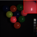
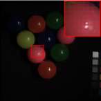
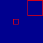
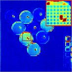
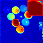
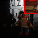
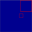
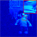
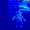
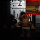
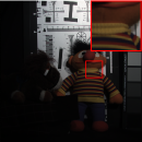
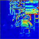
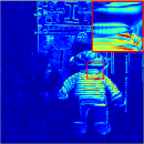
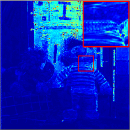
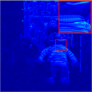
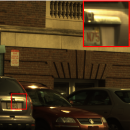
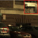
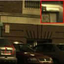
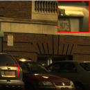
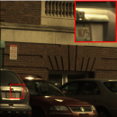
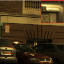
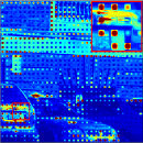
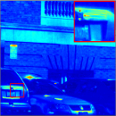
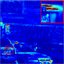
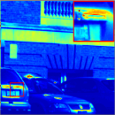
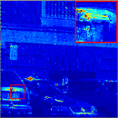
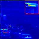
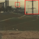
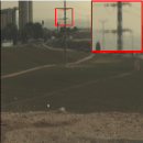
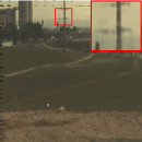
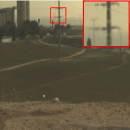
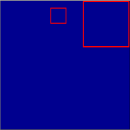
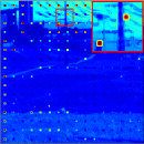
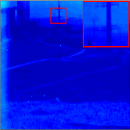
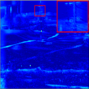
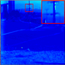
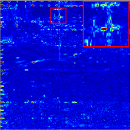
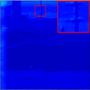
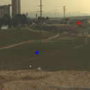
the blur kernel $\mathbf{k}$ and the spectral response function $\mathbf{P}$ are always assumed given for lots of HSI SR methods, which however, is infeasible for the real applications (within above degeneration models, $\mathbf{N_{X}}$ and $\mathbf{N_{Y}}$ are the noise in the observed images, while $\downarrow_{s}$ indicates the down-sampling operation with a scaling factor $s$). Figure 1 gives an example, in which severe reconstruction errors and color distortion exists for NSSR [5] and MHFnet [23] (two state-of-the-art fusion-based HSI SR method) when inaccurate degeneration models are providing. To fill in this gap, some methods turn to estimate the degeneration model from the data first [28, 33, 29, 9], and then utilize it for better HSI SR performance. Despite the advantage estimating the degeneration model from the data, two limitations impede the further improvement of ths kind of HSI SR method. 1) The existing methods estimate the degeneration models with the observed images only, which is hard to obtain an accurate estimation due to the complex and changeable imaging environment. 2) The existing methods estimate the spatial degeneration model only without considering the spectral degeneration model. In these case, these models still will overfit and ultimately degrade their performance on real data.

To address these problems, we investigate how to effectively obtain the degeneration models in both spatial and spectral domain, and makes them can well compatible with the fusion based SR reconstruction model. To this end, we first propose an alternating optimization based deep framework to estimate the degeneration models and reconstruct the latent image, with which the degeneration models estimation and HSI reconstruction can mutually promotes each other. Considering the information can be provided by the observed images is limited, especially for complex blind HSI fusion problem (e.g. HSI SR with a large scaling factor, the given observation images are with heavy noise), we introduce the reconstructed HR HSI with the observed images simultaneously for the degeneration models estimation. Then, a meta-learning based mechanism is further proposed to pre-train the network, which can effectively improve the generalization ability and the speed adapting to different complex degeneration. Extensive experiments report that the proposed method is effective to deal with complex blind HSI fusion problem.

In summary, this study mainly contributes in the following four aspects: 1) We present an alternating optimization based deep framework to effectively estimate degeneration models as well as reconstruct the latent HR HSI. 2) We propose a compact reconstruction network, which can further utilize the information in degeneration models to guide the reconstructing of the latent HSI. 3) We further adopt the meta-learning technology to enhance the generalization ability of the proposed reconstruction network, and improve the speed adapting to different complex degeneration. 4) Extensive experiment results demonstrate the proposed method can achieve state-of-the-art performance in terms of blind HSI fusion SR problem.

2 Related works

2.1 Blind image SR methods

Blind SR methods [7, 30, 18, 9] aim to alleviate the performance drops that caused by the inexact degeneration model. In traditional blind single image (e.g. RGB image) SR (SISR) methods [7, 29, 33, 2], they only need to take care of the spatial degeneration model (i.e. blur kernel $\mathbf{k}$ is unknown). In [9], Hussein et al. propose to utilize a correction filter to match the test images close to the data that generated by known blur kernels (e.g. bicubic). Gu et al. [7] develop a supervised end-to-end network to iteratively estimating the blur kernel and reconstructing the latent image. Though these methods incorporating the estimation of blur kernel into SR, they just utilize the observed images to estimate the blur kernel, which is prone to degrade the performance of complex blind HSI fusion problem (e.g. HSI SR with a large scaling factor, the given observation images are with heavy noise).

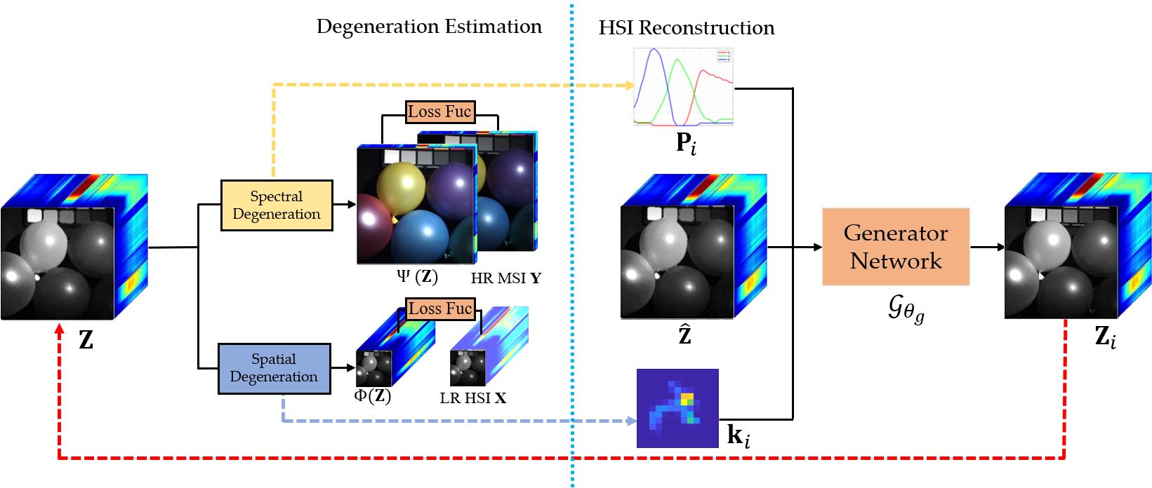
(a) The flowchart of the proposed alternating optimization framework.

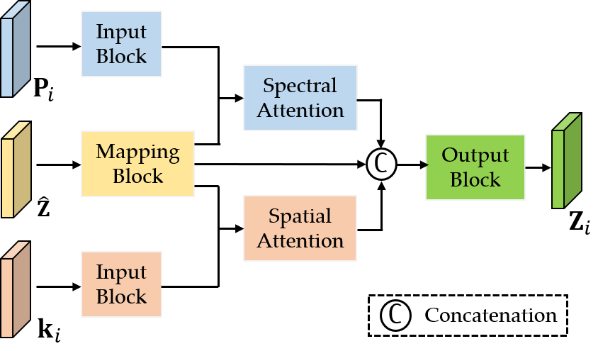
(b) The structure of the reconstruction network.

Figure 2: The flowchart of the proposed method and the proposed reconstruction network. In figure (a), the solid lines indicate the data stream of the network interior and the dotted lines denote the information transformation when alternating optimization.

As for fusion based method, there are few methods [20, 30] taking the blind HSI SR problem into consideration. Wang et al. apply a idea similar as  [7, 29] to train a supervised end-to-end iterative network for solving the blind HSI fusion problem. So far, most of HSI SR methods are supervised which need plenty paired data to train a network. However, the HSI datasets often contain few images which is hard to support large scale supervised training. Therefore, how to unsupervised exploit the image priors [5, 32, 17, 22] that contains in observed images is a promising way to reconstruct the latent HSI. In [30], Zhang et al. propose to joint optimizing the degeneration model and reconstruction model in an unsupervised manner. However, this method demands large amount of computations. In addition, the network builds directly with the observed images without pre-training with the existing available HSI, which thus has a slow training speed and lower generalization ability to complex degradation. In this study, we first parameterize the key components of degeneration model by one single network layer (e.g. 2-D convolution layer), and adopt an unsupervised regularization to train the degeneration models. Then, we introduce the alternating optimization mechanism to optimize the degeneration model and reconstruction model, the experiment results demonstrate that the proposed method can well estimate the degeneration model.

3 Method

3.1 Problem formulation

Unsupervised fusion-based HSI SR method is to inversely reconstruct the latent HR HSI $\mathbf{Z}\in\mathbb{R}^{B\times N}$ by jointly exploiting the LR HSI $\mathbf{X}\in\mathbb{R}^{B\times n}$ and HR MSI $\mathbf{Y}\in\mathbb{R}^{b\times N}$. $B$, $b$ denote the number of spectral bands, $N$, $n$ represent the number of pixels in spatial domain, and $b\ll B$, $n\ll N$. With the degeneration model (i.e. the observation model) described in Eq.(1), a general maximum a posteriori (MAP) estimation is always utilized for fusion-based HSI SR as

$$\min_{\mathbf{Z}}\,\,\,\|\mathbf{X}-(\mathbf{k*Z})\downarrow_{s}\|^{2}+\|\mathbf{Y}-\mathbf{PZ}\|^{2}+\lambda\mathcal{R}(\mathbf{Z}),$$ (2)

where the first two terms are the data fidelity terms, and $\mathcal{R}(\mathbf{Z})$ is the image prior (regularizer) on $\mathbf{Z}$ for optimization. However, the premise of Eq.(2) is that the utilized degeneration models are well consistent with the real ones. Thus, the HSI SR is regarded as a non-blind optimization problem, i.e., the optimization of $\mathbf{Z}$ is accomplished in Eq.(2) without considering the degeneration models.

3.2 Alternating optimization based learning

Recent studies on traditional blind SISR [7, 14, 33] reveals that adding a step of estimating the degeneration model is benefit to promote the performance of blind SR. Following this idea, we can model the blind fusion-based HSI SR method as

$$\left\{\begin{array}[]{l}\mathbf{k}=E_{k}(\mathbf{X}),\quad\mathbf{P}=E_{p}(\mathbf{Y}),\\ \begin{split}\mathbf{Z}=\mathop{\arg\min}\limits_{\mathbf{Z}}\,&\|\mathbf{X}-(\mathbf{k*Z})\downarrow_{s}\|^{2}+\\ &\|\mathbf{Y}-\mathbf{PZ}\|^{2}+\lambda\mathcal{R}(\mathbf{Z}).\end{split}\end{array}\right.$$ (3)

Within this model, we can first estimate the degeneration models by $E_{k}(\cdot)$ and $E_{p}(\cdot)$ from the observed data $\mathbf{X,Y}$, respectively. Then, we can utilize the estimated degeneration models to reconstruct the HR HSI $\mathbf{Z}$. Despite the advantage Eq.(2) estimates both the spatial and spectral degeneration models (i.e., $E_{k}(\cdot)$ and $E_{p}(\cdot)$), the following two limitations impede the further improvement of such a blind fusion-based HSI SR method. First, $E_{k}(\cdot)$ and $E_{p}(\cdot)$ are estimated with the observed images $\mathbf{X,Y}$ only, which is insufficient to obtain an accurate estimation of the degeneration models, especially for complex blind HSI fusion problem (e.g. HSI SR with a large scaling factor, the given observation images are with heavy noise). Second, the estimation of $E_{k}(\cdot)$ and $E_{p}(\cdot)$ is independent with the estimation of $\mathbf{Z}$, which makes the estimated degeneration models still cannot well fit the estimation of $\mathbf{Z}$.

To boost the performance of HSI fusion method, we further propose a blind fusion-based HSI SR method within alternating optimization based framework [14]. First, we reformulate the degeneration models into learnable networks as Eq.(4) for better estimation. Specifically, the spatial degeneration model is reformulate by a network $\Phi(\cdot)$ parameterized by $\mathbf{k}$, which can be implemented by a 2-D convolutional layer with kernel as $\mathbf{k}$. While the spectral degeneration model is reformulated by a network $\Phi(\cdot)$ parameterized by $\mathbf{P}$, which is implemented by a fully connection layer with $\mathbf{P}$ as its parameter. It is noticable that both $\Phi(\cdot)$ and $\Phi(\cdot)$ relate to the HR HSI $\mathbf{Z}$, which provides richer information for estimating the degeneration model as well as integrating the estimation of the degeneration model and estimating $\mathbf{Z}$ into a close loop.

$$\mathbf{X}=\Phi(\mathbf{Z;k})+\mathbf{N_{X}},\quad\mathbf{Y}=\Psi(\mathbf{Z;P})+\mathbf{N_{Y}}.$$ (4)

Then, we can optimize $\mathbf{k}$, $\mathbf{P}$ as well as $\mathbf{Z}$ jointly in one unified framework taking advantages of modeling $\Phi(\cdot)$ and $\Phi(\cdot)$. Considering simultaneously optimizing $\mathbf{k}$, $\mathbf{P}$ as well as $\mathbf{Z}$ is difficult, an alternating optimization based blind HSI SR framework is formulated as

$$\left\{\begin{array}[]{l}\mathbf{k}_{i+1}=\mathop{\arg\min}\limits_{\mathbf{k}}\|\mathbf{X}-\Phi(\mathbf{Z}_{i})\|^{2}+\eta\|\mathbf{k}\|^{2},\\ \mathbf{P}_{i+1}=\mathop{\arg\min}\limits_{\mathbf{P}}\|\mathbf{Y}-\Psi(\mathbf{Z}_{i})\|^{2}+\xi\|\mathbf{P}\|^{2},\\ \begin{split}\mathbf{Z}_{i+1}=\mathop{\arg\min}\limits_{\mathbf{Z}}\,&\|\mathbf{X}-\Phi_{i}(\mathbf{Z})\|^{2}+\\ &\|\mathbf{Y}-\Psi_{i}(\mathbf{Z})\|^{2}+\lambda\mathcal{R}(\mathbf{Z}).\end{split}\end{array}\right.$$ (5)

By alternatively optimizing the degeneration models and the reconstruction model (i.e. optimization of $\mathbf{Z}$), the errors between the estimated degeneration model and the real one can be reduced gradually. Therefore, the reconstruction model can benefit from the exactly estimated degeneration models and thus improve the performance of blind HSI SR.

3.3 Efficient deep HSI reconstruction network with deep image prior

Eq.(5) provides an effective strategy to incorporate the estimation of degeneration models into the reconstruction model. However, the reconstruction model (i.e. optimization of $\mathbf{Z}$) is still challenging due to the ill-posed nature. To well address such an ill-posed inverse problem, proper image priors such as sparsity prior [5, 13] are modeled to regularize the solution of $\mathbf{Z}$ during its optimization. Recently, deep image prior (DIP) [12] is proposed to utilize a generation network to represent the image prior, which shows the state-of-the-art performance for image restoration. The advantage of DIP is that it can capture plenty of low-level statistics which can better reflect the image characteristics and thus well regularize the inverse problem. However, it consumes too much time during optimizing. We analyze the reason as follows. For DIP based SR method [15, 30], it utilizes the random noise for initialization, and then gradually approximates the optimum solution (i.e. the final reconstructed image). Due to the huge differences between the random noise and the optimum solution, the method with DIP will need a complex and deep network as the generator network, which consumes too much time on optimizing. Thus, a natural idea is the difficulty of training as well as the time for optimization can be tremendously decreased if we can provide a good estimated image instead of random noise for initialization.

Therefore, we propose to pre-train a network which can provide a rough reconstructed image as the initial input of the DIP based HSI reconstruction network. Instead of using the observed images for pre-training, we pre-train the network with the existing available amounts of HSI data in the external dataset (e.g. CAVE dataset) since they can provide rich low-level features which always repeatedly appear in different images. For this purpose, we first pre-train a backbone network $\mathcal{F}$ to extract the general image priors within external dataset for roughly reconstructing the latent HSI, which is trained via solving the following problem.

$$\begin{split}\min_{\theta_{f}}\sum_{a,b,c}&\|\mathbf{Z}_{a}-\hat{\mathbf{Z}}_{abc}\|^{2},\,\,{\rm{s.t.}},\hat{\mathbf{Z}}_{abc}=\mathcal{F}(\mathbf{X}_{ab},\mathbf{Y}_{ac};\theta_{f}),\\ &\mathbf{X}_{ab}=(\mathbf{k}_{b}*\mathbf{Z}_{a})\downarrow_{s},\,\,\mathbf{Y}_{ac}=\mathbf{P}_{c}\mathbf{Z}_{a},\end{split}$$ (6)

${\mathbf{Z}_{a}}$ denotes the HSI within the external datasets, while ${\mathbf{X}_{ab}}$ and ${\mathbf{Y}_{ac}}$ are the degenerated images obtained by applying $\mathbf{k}_{b}$ and $\mathbf{P}_{c}$ on ${\mathbf{Z}_{a}}$. $\hat{\mathbf{Z}}_{abc}$ is the roughly reconstructed HR HSI and $\theta_{f}$ is the parameter of the backbone network. Since $\mathcal{F}$ is used for generating a rough reconstructed HSI, most existing HSI fusion networks structure can be adopted as $\mathcal{F}$.

Once obtaining the roughly reconstructed HSI via $\mathcal{F}$, we then utilize it as the initialized input for the generation network of DIP based method. The generation network in this study is termed as the reconstruction network since it is utilized to generate $\mathbf{Z}$. Considering HSI contains both spectral and spatial information, we develop a compact reconstruction network shown as Figure 2(b) to further exploit the additional information contains in $\mathbf{k}$ and $\mathbf{P}$, in which $\mathbf{k}$ and $\mathbf{P}$ provide extra guidance information for the reconstruction network. Specifically, $\mathbf{k}$ is utilized with $\hat{\mathbf{Z}}$ to generate features focusing on spatial information, while $\mathbf{P}$ together with $\hat{\mathbf{Z}}$ aims to generate features relate with spectral information.

Based on above defined backbone as well as the reconstruction network, the alternating optimization based blind HSI fusion model (depicted in Eq.(5)) can be illustrated in Figure 2(a) and further expressed as

$$\left\{\begin{array}[]{l}\mathbf{k}_{i+1}=\mathop{\arg\min}\limits_{\mathbf{k}}\|\mathbf{X}-\Phi(\mathbf{Z}_{i})\|^{2}+\eta\|\mathbf{k}\|^{2},\\ \mathbf{P}_{i+1}=\mathop{\arg\min}\limits_{\mathbf{P}}\|\mathbf{Y}-\Psi(\mathbf{Z}_{i})\|^{2}+\xi\|\mathbf{P}\|^{2},\\ \begin{split}\mathbf{Z}_{i+1}=&\mathop{\arg\min}\limits_{\mathbf{Z},\theta_{g}}\,\|\mathbf{X}-\Phi_{i}(\hat{\mathbf{Z}})\|^{2}+\|\mathbf{Y}-\Psi_{i}(\hat{\mathbf{Z}})\|^{2},\\ &s.t.,\mathbf{Z}=\mathcal{G}(\hat{\mathbf{Z}},\mathbf{k},\mathbf{P};\theta_{g}),\hat{\mathbf{Z}}=\mathcal{F}(\mathbf{X},\mathbf{Y};\theta_{f}),\end{split}\end{array}\right.$$ (7)

where $\mathcal{G}$ denotes the proposed reconstruction network parameterized by $\theta_{g}$.

Considering the potential $\mathbf{k}$ and $\mathbf{P}$ within Eq.(7) is diverse, we finally introduce the meta-learning mechanism [18] to enhance the learning ability of the reconstruction network to different $\mathbf{k}$ and $\mathbf{P}$. To this end, we synthesize plenty of degenerated images from HR HSIs by combining different $\mathbf{k}$ and $\mathbf{P}$, and forming these data into a meta-learning training dataset $\mathcal{M}$. Then, we pre-train the reconstruction network via the Model-Agnostic Meta-Learning (MAML) method proposed in [6], in which the meta-objective function is defined as

$$\mathop{\arg\min}\limits_{\theta_{g}}\sum_{\mathcal{M}_{j}\sim p(\mathcal{M})}\mathcal{L}_{\mathcal{M}_{j}}^{te}(\theta_{g}-\alpha\nabla_{\theta_{g}}\mathcal{L}_{\mathcal{M}_{j}}^{tr}(\theta_{g})),$$ (8)

$\mathcal{L}_{\mathcal{M}_{j}}^{te}$ and $\mathcal{L}_{\mathcal{M}_{j}}^{tr}$ denote the loss of test and training on sub-task $\mathcal{M}_{j}$, and $\alpha$ is the task-level learning rate. With the meta-learning mechanism, we can obtain a better initialization value of the reconstruction network $\mathcal{G}$, which results in better generalization ability and faster learning speed. The details analysis can be seen from the ablation study.

4 Experimental results and analysis

4.1 Experimental settings

Datasets In this study, we utilize two benchmark HSI datasets and one real HSI dataset to testify the effectiveness of the proposed method, including CAVE [27], Harvard [3] and HypSen [26]. Specifically, the CAVE dataset contains 32 indoor HSIs and each of which has 31 spectral bands covering the wavelength range from 400 $nm$ to 700 $nm$ with a 10 $nm$ interval. Meanwhile, each HSI in the CAVE dataset contains $512\times 512$ pixels in the spatial domain. The Harvard dataset includes 50 HSIs containing both indoor and outdoor scenes. Each HSI in the Harvard dataset also has 31 bands in a wavelength range from 420 $nm$ to 720 $nm$, and $1392\times 1300$ pixels in spatial domain. Different with the above two datasets, HypSen is a real fusion-based HSI dataset containing a 10m-resolution MSI and a 30m-resolution HSI. After removing the noisy bands as well as the water-absorbed bands as [26], the resulted LR HSI includes 84 spectral bands and HR MSI consists of 13 spectral bands. In the experiment on the HypSen dataset, a sub-image with $250\times 330$ spatial size is cropped from the LR HSI and the one with $750\times 990$ spatial size is cropped from the HR MSI.

Comparison methods and Evaluation Metrics In this study, due to the lack of blind fusion-based HSI SR method, five state-of-the-art fusion-based HSI SR methods including two non-blind method, two semi-blind method and one blind method are utilized for comparison. The first two methods are non-blind HSI fusion methods, in which NSSR [5] is a non-deep unsupervised method with optimization, and MHFnet [23] is a supervised deep learning based method. Yong [13] and UAL [31] are semi-blind methods, in which $\mathbf{P}$ is provided and only $\mathbf{k}$ of the spatial degeneration is unknown. The last method DBSR [30] is a DIP [12] based unsupervised blind method, which simultaneous optimize the degeneration estimation as well as the HSI reconstruction within a jointly framework.

Four quantitative metrics including root-mean-square error (RMSE), peak signal-to-noise ratio (PSNR), spectral angle mapper (SAM) and structural similarity index (SSIM) is utilized to evaluate the SR performance.

Implementation details  In the experiments, the HSIs in CAVE and Harvard datasets are regarded as the ground truth of the latent HR HSI $\mathbf{Z}$. The corresponding LR HSI and HR MSI for pre-training in these two datasets are generated from the latent HR HSI $\mathbf{Z}$ based on Eq (1), among which the spectral response function of Nikon D700 camera in [5, 13] and Gaussian kernel is adopted as $\mathbf{k}$ and $\mathbf{P}$.

$$\mathbf{P}_{c}=Softmax(\mathbf{P}+c).$$ (9)

For the observed images $\mathbf{X}$ and $\mathbf{Y}$, we generate them with the blur kernels and the spectral response function, different with $\mathbf{k}$ and $\mathbf{P}$ utilized for the pre-training data. Specifically, four different motion kernels includes $\mathbf{k_{1}}$, $\mathbf{k_{2}}$, $\mathbf{k_{3}}$ and $\mathbf{k_{4}}$ (shown in the Figure 5) instead of Gaussian kernel to generate the observed LR HSI $\mathbf{X}$. While, Eq (9) is utilized to generate the spectral response matrix $\mathbf{P_{c}}$ of the observed HR MSI, in which $c$ is a transform coefficient and $\mathbf{P}$ is the spectral response matrix for pre-train. In addition, to simulate the noise disturbance, we add Additive White Gaussian Noise with different intensities into the observed image $\mathbf{X}$ and $\mathbf{Y}$. Some other detailed settings are given in the supplement due to the limitations of page length.

Table 1: The performance of each method on the CAVE dataset with different settings. SNR of both two observed images are 40dB, and the SR scale is 8. In experiments, the input LR HSI and HR MSI are generated by $\mathbf{k}_{1}$ and $\mathbf{P}_{0.02}$, respectively. The best results are in bold.

Methods	RMSE	PSNR	SAM	SSIM
Ours_Sep	5.72	34.13	8.98	0.9629
Ours_Joint	3.87	37.06	6.95	0.9828
Ours_Alter	2.97	39.38	6.75	0.9838
Ours_Basic	3.03	39.19	6.80	0.9841
Ours	2.86	39.74	6.64	0.9845

Table 2: The performance of each method on the CAVE dataset with different SR scale factors. The best results are in bold.

Methods	s = 8				s = 16				s = 32
	RMSE	PSNR	SAM	SSIM	RMSE	PSNR	SAM	SSIM	RMSE	PSNR	SAM	SSIM
NSSR [5]	8.11	30.53	18.85	0.8533	8.31	30.27	14.75	0.8976	7.87	30.68	15.89	0.8287
MHFnet [23]	4.53	35.67	14.01	0.9409	4.74	35.44	11.75	0.9547	5.17	34.80	12.85	0.9524
Yong [13]	4.46	35.72	11.29	0.9491	4.98	34.88	11.80	0.9468	6.34	32.72	14.04	0.9318
UAL [31]	3.93	37.07	7.57	0.9724	4.12	36.59	8.06	0.9704	4.59	35.61	9.21	0.9652
DBSR [30]	4.01	36.66	5.53	0.9739	5.10	34.32	9.80	0.9482	8.96	29.49	13.95	0.9054
Ours	2.40	41.12	6.53	0.9854	2.67	40.27	6.93	0.9838	3.47	38.41	8.46	0.9755

(a) GT

(b) NSSR [5]

(c) MHFnet [23]

(d) Yong [13]

(e) UAL [31]

(f) DBSR [30]

(g) Ours

Figure 3: The visual SR results of all methods on the CAVE dataset. The input LR HSI and HR MSI are generated by $\mathbf{k}_{1}$ and $\mathbf{P}_{0.01}$, respectively. SNRs of both two observed images are 40dB, and the SR scale is 8.

4.2 Ablation studies

The proposed method contains three main components: 1) alternating optimization based framework; 2) the modeled compact reconstruction network (shown as Figure 2(b)) incorporating the information contains $\mathbf{k}$ and $\mathbf{P}$; 3) meta-learning for pre-training the reconstruction network.

To demonstrate the advantage of the utilized alternating optimization framework, we compare it with other two commonly used optimization manners, including a two-step based optimization method and jointly optimization method. Specifically, without using the meta-learning strategy for pre-training the reconstruction network, we separately utilize these two kind of optimization manners and the proposed alternating framework to optimize the degeneration model as well as the reconstruction network, and summarize the results on CAVE dataset in Table 1. These three kind of methods are termed as ’Ours_Sep’, ’Ours_Joint’ and ’Ours_Alter’ in this study respectively. As can be seen, the results from ’Ours_Sep’ is the worst among three kind of methods. This is because separately estimating the degeneration model and the reconstruction model provides an inexactly estimated degeneration model for the reconstruction model, which thus inferiors to those from ’Ours_Joint’ which jointly optimizing the degeneration model and the reconstruction model. ’Ours_Alter’ obtains better results compared with those from ’Ours_Joint’, which demonstrates that the alternating optimization method proposed in this study is more beneficial for blind HSI SR.

To testify the modeled compact reconstruction network, we compare the proposed method with its variant (termed as Ours_Basic), in which $\mathbf{k}$ and $\mathbf{P}$ are removed from the input of the reconstruction network. It can be seen that the proposed reconstruction network suffers obvious degradation without the guidance information provided by $\mathbf{k}$ and $\mathbf{P}$. ’Ours’ is the proposed method. Since the only difference between ’Ours’ and ’Ours_Alter’ is the meta-learning strategy for pre-training, the advantage of meta-learning can be seen by comparing ’Ours’ with ’Ours_Alter’.

4.3 Performance comparison on the CAVE dataset

In this Subsection, we compare the proposed method with five competing state-of-the-art methods on the CAVE dataset under different settings including experiments with different SR scale, experiments with different spectral response matrix $\mathbf{P}_{c}$, experiments with different blur kernels.

Different SR scales In this experiment, we generate the observed LR HSI $\mathbf{X}$ and HR MSI $\mathbf{Y}$ with the kernel $\mathbf{k}_{1}$ and the spectral response matrix $\mathbf{P}_{0.01}$, respectively, and add noise into $\mathbf{X}$ and $\mathbf{Y}$, in which SNRs of both observed images are 40dB. We then testify the applicability of all methods with different SR scale factors (i.e. up-sampling the LR HSI for 8, 16, 32 times) and summarize the numerical results in Table 2. It can be seen that the proposed method has obvious advantage over other competing methods on all three SR scales. The PSNR of the proposed method even surpasses the second best method almost for 3dB. Non-blind methods including NSSR [5] and MHFnet [23] present severe performance degradation on the blind settings, especially with a larger SR scale. In contrast, the semi-blind methods including Yong [13] and UAL [31] have better performance. In addition, the performance of the blind competing method DBSR [30] inferiors to the proposed method. We attribute the reason to the optimization method DBSR [30] utilized, which cannot provide a good degeneration model and consequently resulting in the performance degradation. For better comparison, we also provide the visual results of all methods in Figure 3. The first row of Figure 3 provides the pseudo color image of reconstructed HSIs and the second row shows the reconstruction error maps of all methods. It can be seen that the reconstructed HSI of the proposed method has lower reconstruction errors, which is consistent with those in Table 2.

Table 3: The performance of each method on the CAVE dataset with HR MSI generated by different $\mathbf{P}_{c}$ ($c=0.01,0.015,0.02$). The best results are in bold.

	Method	RMSE	PSNR	SAM	SSIM
$\mathbf{P}_{0.01}$	NSSR [5]	8.11	30.53	18.85	0.8533
	MHFnet [23]	4.53	35.67	14.01	0.9409
	Yong [13]	4.46	35.72	11.29	0.9491
	UAL [31]	3.93	37.07	7.57	0.9724
	DBSR [30]	4.01	36.66	5.53	0.9739
	Ours	2.40	41.12	6.53	0.9854
$\mathbf{P}_{0.015}$	NSSR [5]	8.34	30.28	19.08	0.8481
	MHFnet [23]	7.00	32.07	16.50	0.9121
	Yong [13]	5.07	34.70	12.05	0.9421
	UAL [31]	4.96	35.23	8.40	0.9671
	DBSR [30]	4.71	35.65	5.65	0.9733
	Ours	2.59	40.51	6.66	0.9848
$\mathbf{P}_{0.02}$	NSSR [5]	8.56	30.05	19.28	0.8438
	MHFnet [23]	7.43	31.54	16.94	0.9072
	Yong [13]	5.50	34.04	12.79	0.9349
	UAL [31]	5.76	34.03	9.06	0.9629
	DBSR [30]	5.22	34.79	5.83	0.9722
	Ours	2.86	39.74	6.64	0.9845

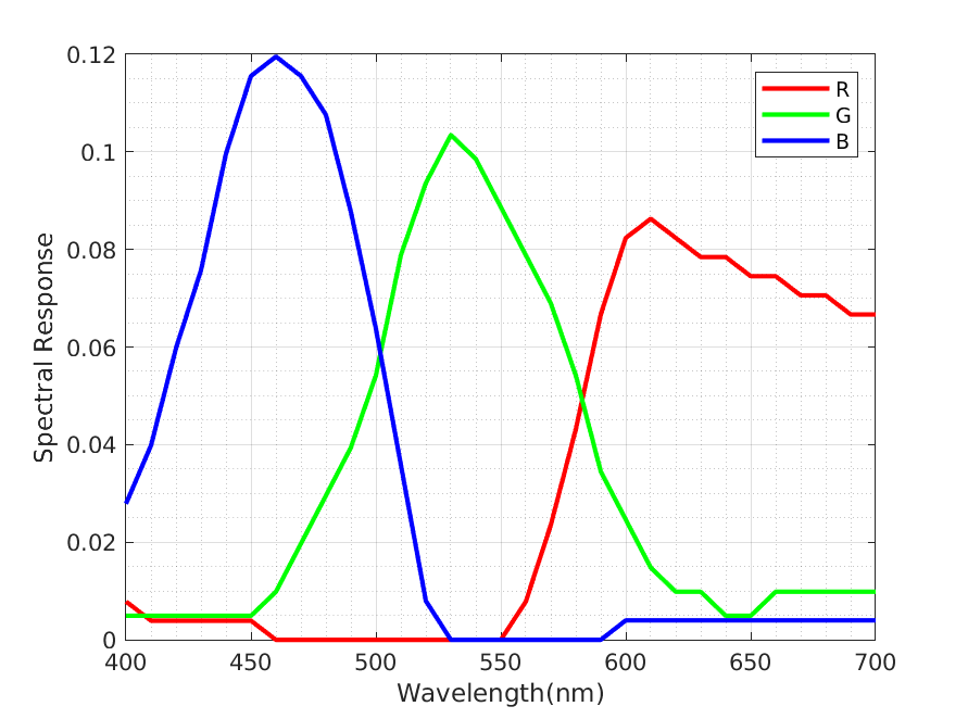
(a) The default spectral response matrix

(b) The spectral response of blue band

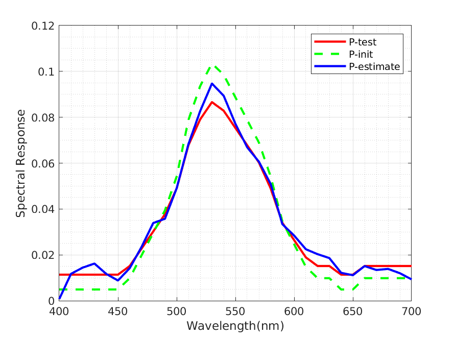
(c) The spectral response of green band

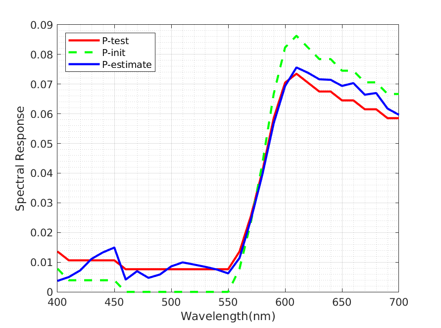
(d) The spectral response of red band

Figure 4: The default spectral response matrix $\mathbf{P}$ as well as the estimated spectral response matrix by the proposed method. (a) the default spectral response matrix $\mathbf{P}$. (b)(c)(d) represent the estimate spectral response metrics for the blue, green and red band.

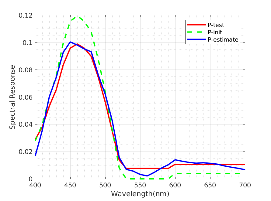
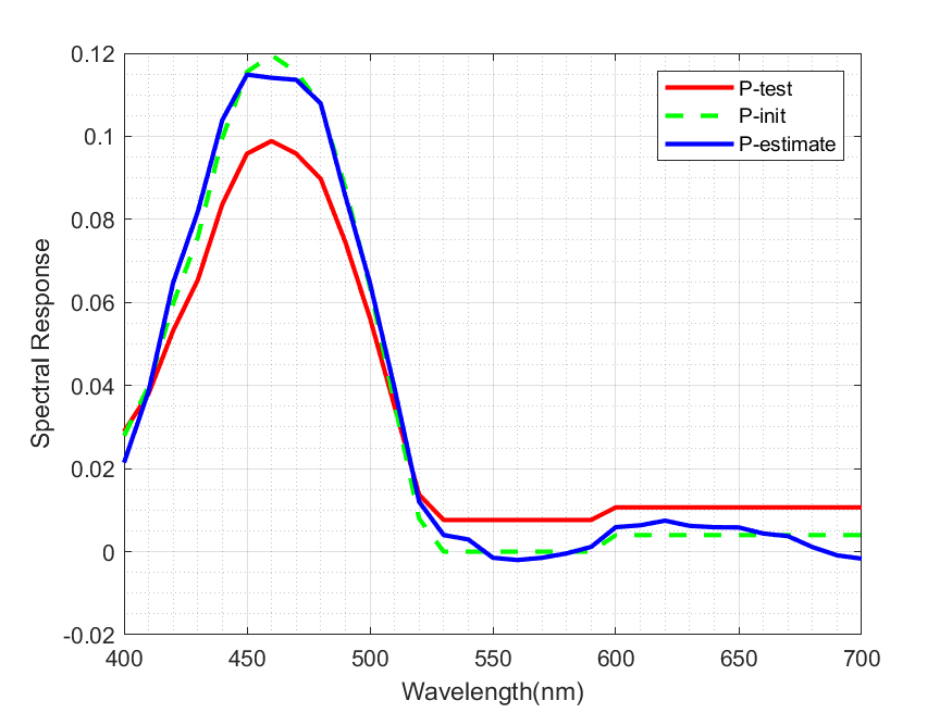
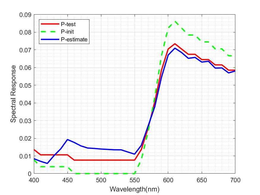
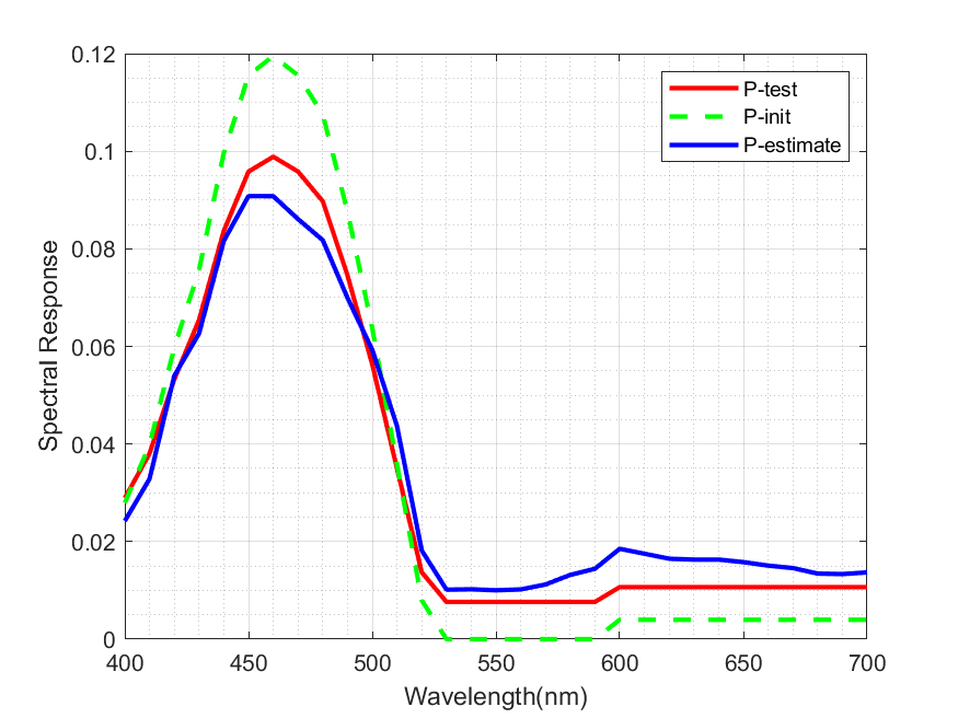
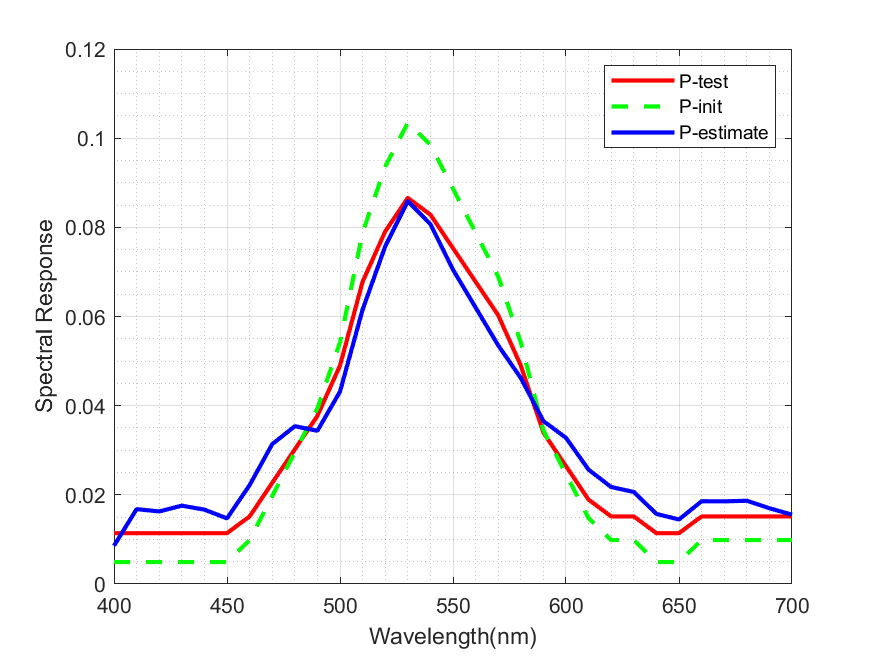
Different spectral response matrix In this experiment, we further explore the performance of the proposed method influenced by the spectral response matrix $\mathbf{P}_{c}$ with different transform coefficient. The blur kernel is $\mathbf{k}_{1}$ and the SR scale is 8. SNRs of both the observed LR HSI and HR MSI are 40dB. The detailed numerical results are summarized in Table 3. It can be be seen that the difficulty of HSI SR is increased with larger transformation coefficient $c$. With the increasing of $c$, the performance of both non-blind methods (i.e. NSSR [5] and MHFnet [23]) and semi-blind methods (i.e. Yong [13] and UAL [31] which consider the degeneration only in spatial domain) degrade severely. The blind method DBSR [30] as well as the proposed method present much robust performance when $c$ increases. Nevertheless, the proposed method still has advantage over DBSR [30] on three out of all four evaluation metrics. The true spectral response matrix utilized as well as the one estimated by the proposed method are visualized in Figure 4. In Figure 4, P-test denotes the $\mathbf{P}_{c}$ that used to generate the observed HR MSI, $c$ is 0.01. P-init is the default spectral response matrix $\mathbf{P}$ and is utilized as the initial parameter of $\Psi$. P-estimate is the estimated spectral response matrix. It can be seen that the proposed method can well estimate the spectral response matrix.

Table 4: The performance of each method on the CAVE dataset with different blur kernel $\mathbf{k}$. The best results are in bold.

	Method	RMSE	PSNR	SAM	SSIM
K1	NSSR [5]	8.11	30.53	18.85	0.8533
	MHFnet [23]	4.53	35.67	14.01	0.9409
	Yong [13]	4.46	35.72	11.29	0.9491
	UAL [31]	3.93	37.07	7.57	0.9724
	DBSR [30]	4.01	36.66	5.53	0.9739
	Ours	2.40	41.12	6.53	0.9854
K2	NSSR [5]	9.26	29.44	19.24	0.8384
	MHFnet [23]	4.59	35.59	14.05	0.9403
	Yong [13]	4.46	35.77	10.78	0.9510
	UAL [31]	3.94	37.05	7.59	0.9424
	DBSR [30]	4.39	36.26	5.54	0.9740
	Ours	2.44	41.17	6.48	0.9858
K3	NSSR [5]	7.50	31.23	18.50	0.8592
	MHFnet [23]	4.52	35.69	14.06	0.9405
	Yong [13]	4.42	35.84	11.17	0.9486
	UAL [31]	3.94	37.03	7.58	0.9722
	DBSR [30]	4.40	36.41	5.62	0.9745
	Ours	2.45	41.03	6.46	0.9862
K4	NSSR [5]	8.30	30.37	18.76	0.8503
	MHFnet [23]	4.55	35.65	14.02	0.9406
	Yong [13]	4.50	35.72	11.16	0.9472
	UAL [31]	3.95	37.02	7.59	0.9722
	DBSR [30]	4.74	35.71	5.53	0.9738
	Ours	2.57	40.68	6.51	0.9857

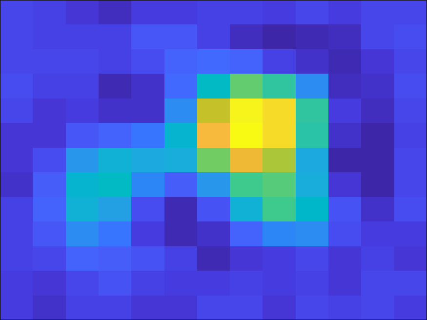
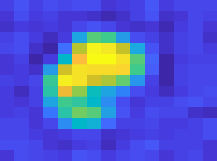
(a) $\mathbf{k}_{1}$

(b) $\mathbf{k}_{2}$

(c) $\mathbf{k}_{3}$

(d) $\mathbf{k}_{4}$

Figure 5: The utilized true blur kernels (the first row) as well as the estimated blur kernels (the second row) by the proposed method.

Table 5: The performance of each method on the Harvard dataset with different SR scale factors. The best results are in bold.

Methods	s = 8				s = 16				s = 32
	RMSE	PSNR	SAM	SSIM	RMSE	PSNR	SAM	SSIM	RMSE	PSNR	SAM	SSIM
NSSR [5]	6.80	32.01	3.85	0.9320	7.05	31.73	5.47	0.9298	6.69	32.25	6.03	0.9463
MHFnet [23]	4.80	35.23	5.47	0.9712	4.84	35.18	5.66	0.9698	5.03	34.85	5.78	0.9688
Yong [13]	3.15	38.73	3.47	0.9670	3.37	38.20	3.72	0.9675	3.68	37.49	4.20	0.9685
UAL [31]	7.06	32.19	6.00	0.9547	6.92	32.25	6.06	0.9530	6.57	32.63	6.11	0.9492
DBSR [30]	4.40	36.14	2.48	0.9660	5.58	34.31	2.87	0.9592	10.06	28.93	3.59	0.9359
Ours	2.37	41.22	2.53	0.9803	2.59	40.40	3.06	0.9787	3.04	39.10	3.40	0.9757

(a) Bicubic

(b) NSSR [5]/12.84

(c) MHFnet [23]/11.19

(d) Yong [13]/12.47

(e) UAL [31]/10.98

(f) DBSR [30]/12.40

(g) Ours/10.87

Figure 6: The visual SR results of all methods on the real dataset HypSen.

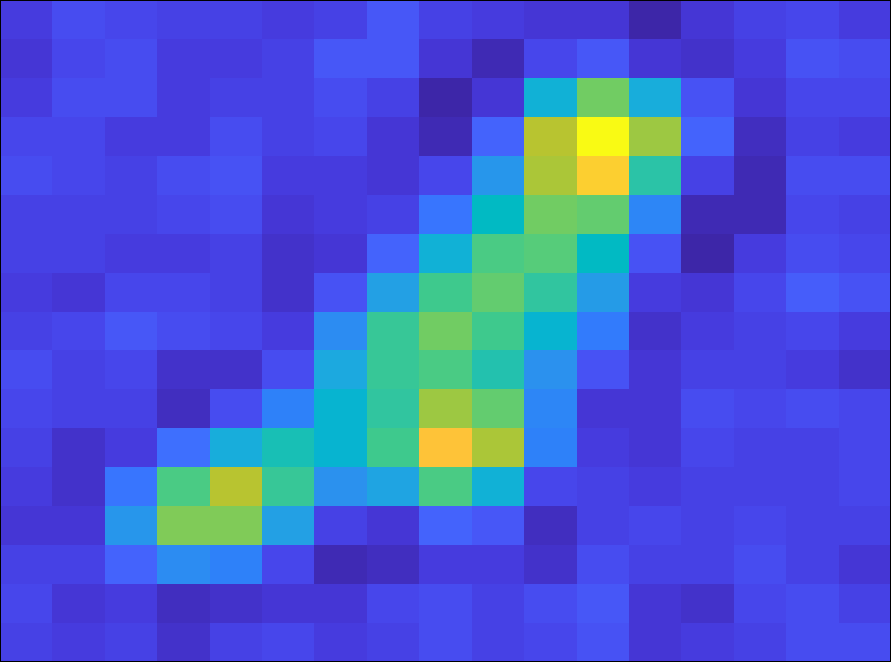
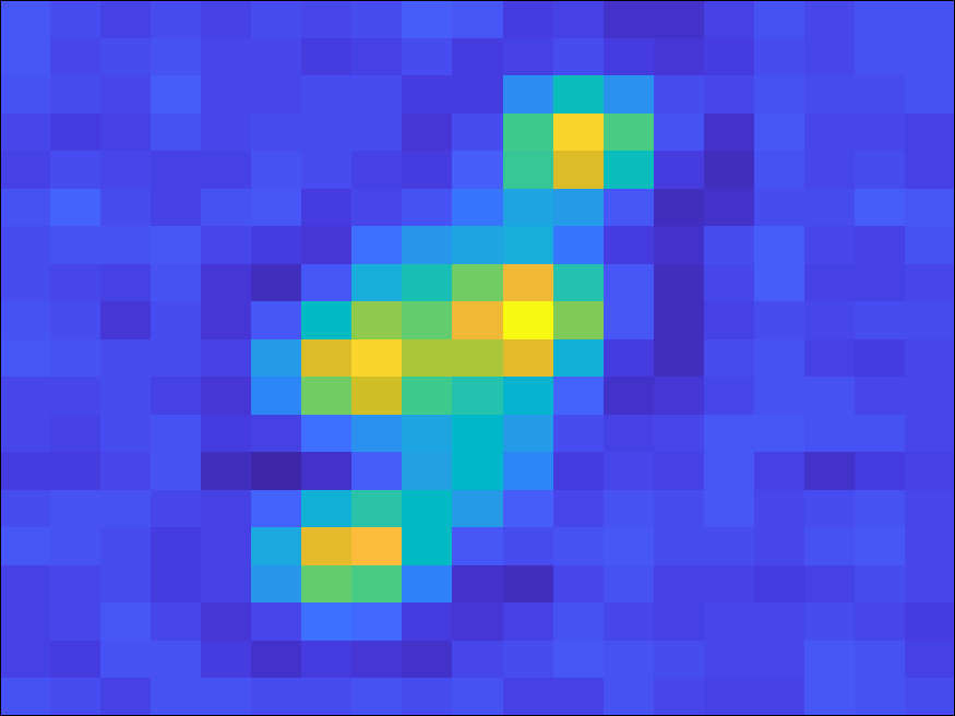
Different blur kernels In this experiment, we further testify the performance of the proposed method influenced by different blur kernels and summarize the experimental results in Table 4. To visualize the accuracy of the estimated kernel, we further display the utilized true blur kernels as well as the estimated blur kernels in Figure 5. In experiments, $\mathbf{P}_{0.01}$ is adopted as the spectral response matrix. SNRs of both the observed LR HSI and HR MSI are 40dB. From the experimental results, we can see that the proposed method can better reconstruct the HR HSI as well as accurately estimate the blur kernels, compared with those from other competing methods.

Besides these three experiments, another experiment is further conducted to verify the performance of the proposed method influenced by the noisy observation images with different intensity of noise. The proposed method still has obvious superiority over other methods, which can be seen from the supplement for detail. From all these experiments, we can conclude the proposed method obtains best performance in both accuracy and robustness.

4.4 Performance comparison on the other datasets

In this Subsection, we further conduct the experiments on the Harvard dataset and a real dataset HypSen dataset to verify the applicability of the proposed method to other datasets.

Performance on the Harvard dataset In this experiment, we compare the proposed method with other competing methods with different SR scales. The observed LR HSI and HR MSI are generated by $\mathbf{k}_{1}$ and $\mathbf{P}_{0.01}$, respectively. SNRs of both these two observed images are 40dB. The detailed numerical results are reported in Table 5. Similar as the results on CAVE dataset, the results of the proposed method on Harvard dataset also has obvious advantages over the comparison methods. The visualization results of all methods on the Harvard dataset is consistent with the result given in Table 5, which can be seen from the supplement for the details.

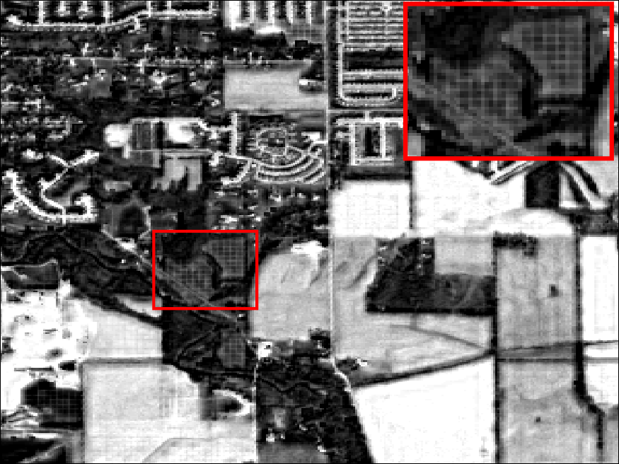
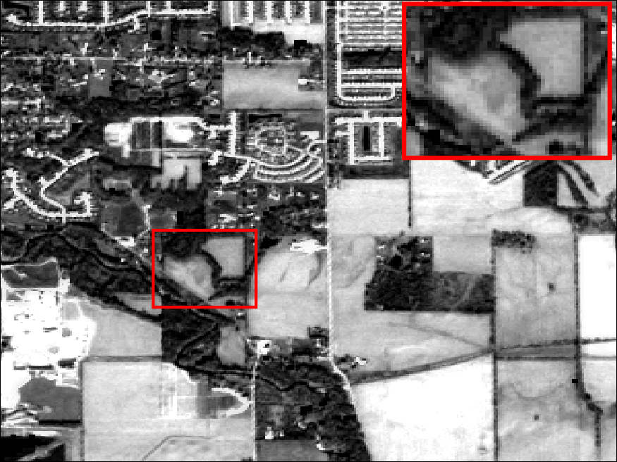
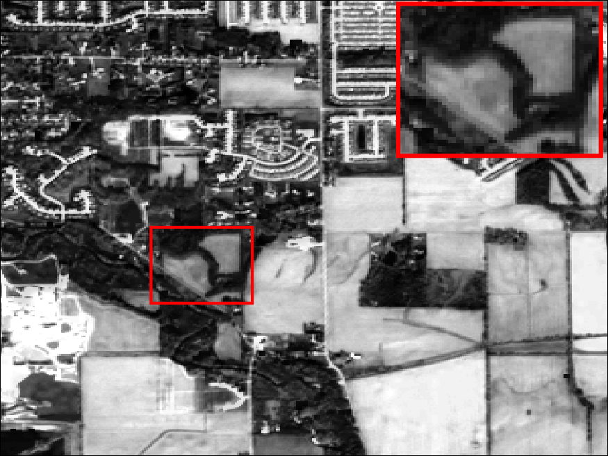
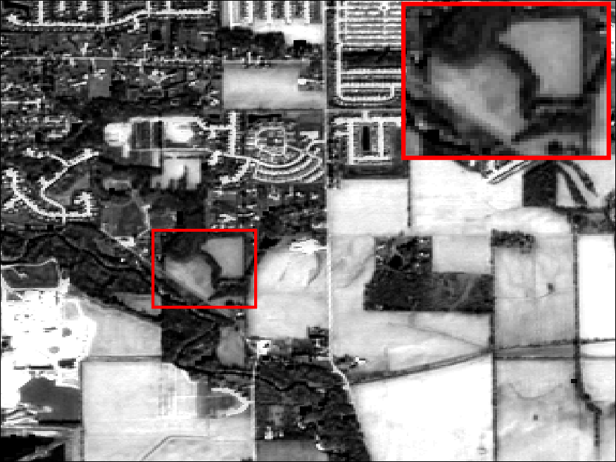
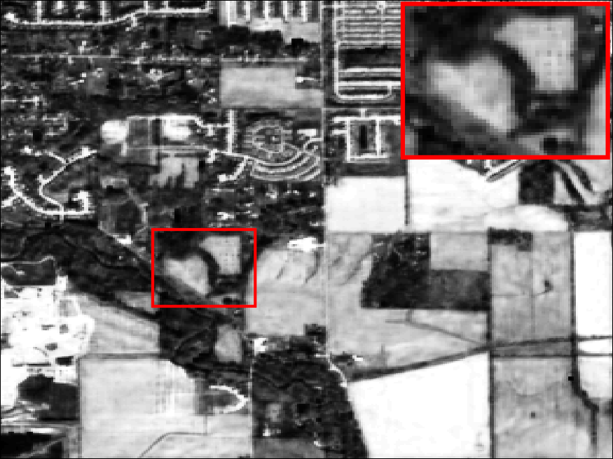
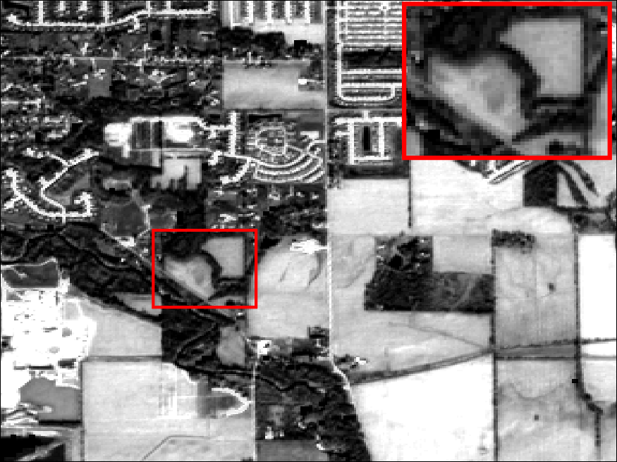
Performance on the Real dataset In this experiment, we verify the proposed method on the real HypSen dataset without knowing the HR HSI. The visualization of reconstructed HSIs of all methods are shown in Figure 6, in which Figure 6(a) is the result directly up-sampling from the LR HSI via bicubic interpolation. It can be seen that the proposed method can well reconstruct the HSI and preserve the image details. In addition, we also measure the reconstruction quality for each method via the no-reference HSI evaluation metric [25] and list the obtained score in the legend of Figure 6. Smaller score represents better results. Thus, it can be seen that the proposed method obtains best performance from both the reconstructed image and the obtained scores.

In summary, we can conclude that the proposed method can applicable to different datasets, which further demonstrates the effectiveness of the proposed method for HSI SR.

4.5 Runtime analysis

In the Table 6 we summarize the average runtime of all the methods. The non-deep methods (i.e. NSSR [5] and Yong [13]) are run on a workstation with Intel Xeon E5-2640 CPU and 128G memory. The other methods are deep learning based methods, we run them on the same workstation with GeForce GTX 1080ti GPU. The Table 6 demonstrates that the proposed method is faster than most unsupervised methods, especially DBSR [30] which requires almost 2900 second to reconstruct one single HSI.

Table 6: Average runtime of all methods on CAVE dataset when SR scale is 8.

Method	NSSR [5]	MHFnet [23]	Yong [13]	UAL [31]	DBSR [30]	Ours
Time (s)	98.70	2.77	373.98	20.64	2899.80	32.40

5 Conclusion

In this study, we explore an unsupervised blind HSI fusion SR method, which can effectively estimate the degeneration models in spatial and spectral domain, respectively. To this end, we first propose an alternating optimization based deep framework to estimate the degeneration models and reconstruct the latent image, which makes them can mutually promotes each other. A compact reconstruction network is further designed to utilize the information containing in degeneration models. Additionally, we use a meta-learning based training mechanism to further pre-train the reconstruction network to make the proposed reconstruction network can fast adapt to different complex degeneration. Experiments on two benchmark HSI SR datasets and one real dataset demonstrate the proposed method is effective for the blind HSI SR.

6 Implementation details

In this material, we further supplement the details of the training and testing, as well as more experimental results of the proposed method.

6.1 Training details of backbone network

In the submitted manuscript, we propose to pre-train a backbone network $\mathcal{F}$ first, aiming to exploit the general image priors contained in the existing available amounts of HSI data. Since the pre-trained network $\mathcal{F}$ we utilized is to generate a rough reconstructed HSI as the initial input for the reconstruction network, most of the existing fusion based HSI network can be adopted as the backbone network. In this work, we select a multi-branch network [31] as the $\mathcal{F}$ to jointly exploit the general spatial-spectral information that contain in the available HSI data.

We separate each benchmark dataset into training set and testing set. Specifically, we select 12 HSIs, 15 HSIs, 20 HSIs from the CAVE dataset, the Harvard dataset and NTIRE [8575282] dataset as the training data, respectively, and the remaining data within these datasets are left for test. NTIRE dataset is a newly introduced dataset. It has 255 HSIs each has $1392\times 1300$ pixels in spatial domain and 31 bands covering the wavelength range from 400nm to 700nm.

To pre-train the backbone network, we crop the HSIs from the training set into overlapping patches with spatial size as $128\times 128$ and stride as 64, and then utilize cropped HSIs to generate the corresponding LR HSI and HR MSI. It is noticeable that the spectral and spatial degeneration models we utilized to generate the LR HSI and HR MSI are different with those utilized in test. Specifically, the bluer kernel $\mathbf{k}$ is initialed with the Gaussian distribution, which kernel size and standard deviation are randomly chosen within the ranges [5, 15] and [0.5, 2], respectively. In addition, $c$ used for the spectral response matrix (i.e., spectral degeneration model) is chosen within the range [5e-3, 8e-3]. Once obtaining the LR HSI and HR MSI, we train the backbone network $\mathcal{F}$ by setting a $\ell_{1}$ norm based loss and Adam optimizer [11]. The learning rate is initialized as 1e-4 and decreased every 10 epochs by 0.7. The maximum training epoch is 150 and the batchsize is set as 6. All deep models for the proposed method including the backbone network are implemented by the Pytorch [16] deep learning framework.

6.2 Training details of meta-learning

We first utlize the LR HSI and HR MSI for pre-training $\mathcal{F}$ in order to generate the rough reconstructed HSI $\hat{\mathbf{Z}}$. Then the $\hat{\mathbf{Z}}$ will be input to the alternating optimization based framework for meta-learning. The manner of generating the meta-learning dataset $\mathcal{M}$ is same as that for the backbone network. The meta-learning is conducted for 100 epochs, with initial task-level learning rate as 1e-3 and halved after every 10 epochs. Due to the spatial and spectral degeneration networks only contain few learnable parameters, thus, the meta-learning mechanism can not brings obvious improvements on it. Therefore, we adopt the default blur kernel and spectral response matrix as the initial parameters of them, respectively.

6.3 The details for the test

In the test phase, we first input the test LR HSI and HR MSI (without cropped) into the pre-trained backbone network $\mathcal{F}$, then input the obtained $\hat{\mathbf{Z}}$ into the degeneration network as the $\mathbf{Z}_{0}$, from which the parameters $\mathbf{k}_{0}$ and $\mathbf{P}_{0}$ related with the spatial and spectral degeneration network can be extracted. The obtained $\mathbf{k}_{0}$ and $\mathbf{P}_{0}$ are then combined with $\hat{\mathbf{Z}}$ be utilized to reconstruct the $\mathbf{Z}_{1}$ via the reconstruction network, from which the degeneration models and the reconstruction network are related. Finally, we optimize the degeneration models and the reconstruction network via the proposed alternating optimization framework. In the test phase, We also adopt the Adam algorithm [11] as the optimizer and $\ell_{1}$ norm based loss function to optimize the degeneration network and the meta-learning pre-trained reconstruction network. The learning rate of these two parts are 1e-4 and 1e-3, respectively. The total iteration number is 400, in which the outer-loop iteration number and the inner-loop iteration number is set as 40 and 10 in the experiment, respectively.

7 More Experiments

Table 7: The performance of each method on the CAVE dataset with input images, which suffers from noise with different intensities. The best results are in bold.

Noise intensity	Method	RMSE	PSNR	SAM	SSIM
k1	Ours_Sep	5.72	34.13	8.98	0.9629
	Ours_Joint	3.87	37.06	6.95	0.9828
	Ours_Alter	2.97	39.38	6.75	0.9838
k2	Ours_Sep	5.84	33.97	9.10	0.9628
	Ours_Joint	3.96	36.84	7.08	0.9819
	Ours_Alter	3.01	39.27	6.80	0.9837
k3	Ours_Sep	5.69	34.21	8.99	0.9625
	Ours_Joint	4.30	36.26	7.03	0.9809
	Ours_Alter	3.33	38.58	6.75	0.9833
k4	Ours_Sep	5.74	34.16	8.99	0.9625
	Ours_Joint	4.18	36.48	7.00	0.9816
	Ours_Alter	3.03	39.41	6.76	0.9832

7.1 Ablation study

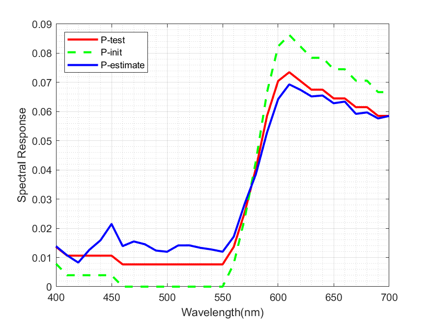
Effect of the optimization manner In the main manuscript, we have provided partial results to demonstrate the superiority of the alternating optimization framework. In this Subsection, we supplement an ablation study to further compare the performance of different optimization manners (e.g. Our_Sep, Our_Joint and Our_Alter). Specifically, we testify these three methods using all four motion kernels with $\mathbf{P}_{0.02}$ as the test spectral response matrix. SNRs of both the observed LR HSI and HR MSI are 40dB and the SR scale is 8. The detailed numerical results are reported in the Table 7. It can be seen the performance of alternating optimization based method is obvious superior to the other two kind of optimization manners, which is consistent with the conclusion in the main manuscript. In addition, we further plot the estimated blur kernels (e.g. Figure 7) and the spectral response matrices (e.g. Figure 8) of these three kinds of methods. It can be seen that though all these three kind of methods can estimate the kernel with a similar shape as the test one, the estimated kernels of Ours_Joint and Ours_Sep are much fuzzier than that estimated by Ours_Alter. The estimated spectral response matrices shown in the Figure 8 also demonstrate the Ours_Sep inferiors to the other two kinds of methods. Furthermore, the Ours_Alter can well estimate the degeneration models in both spectral and spatial domains, thus presents a better performance than Ours_Joint on blind HSI fusion SR.

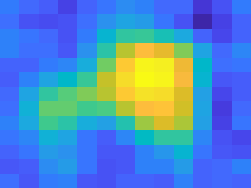
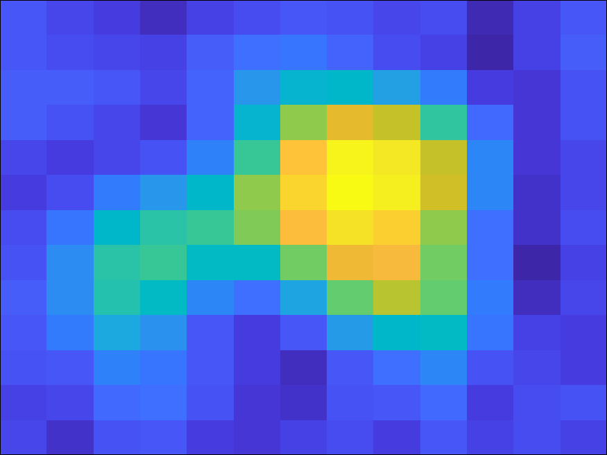
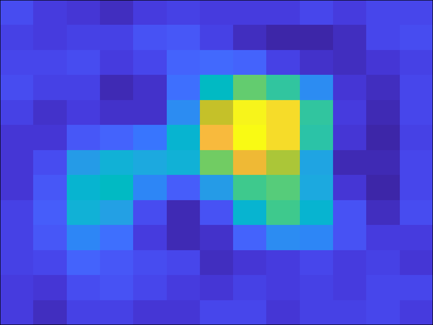
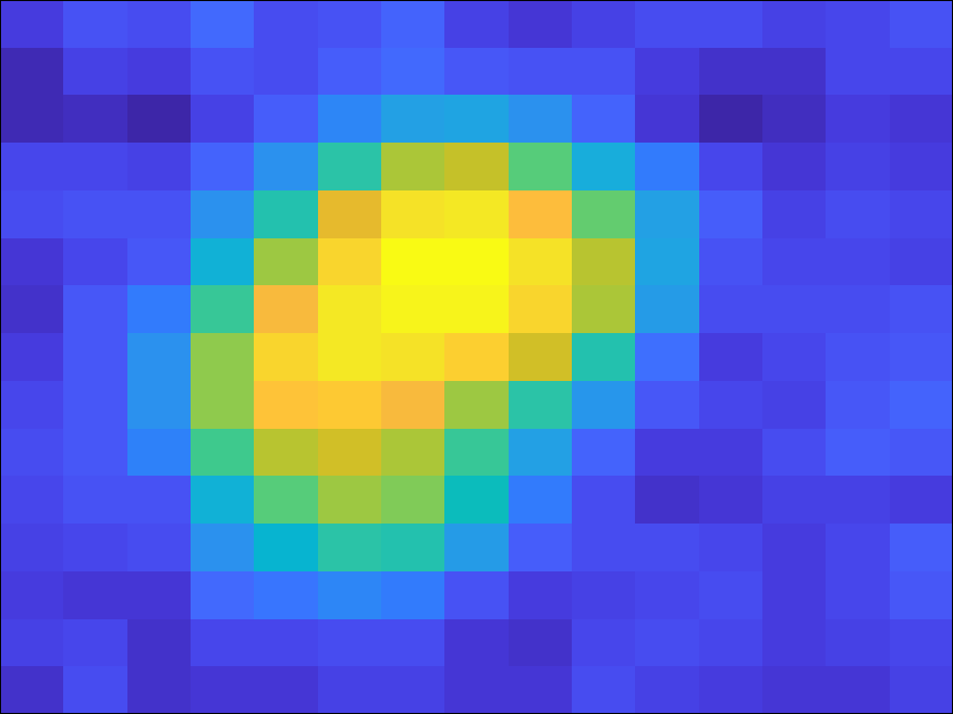
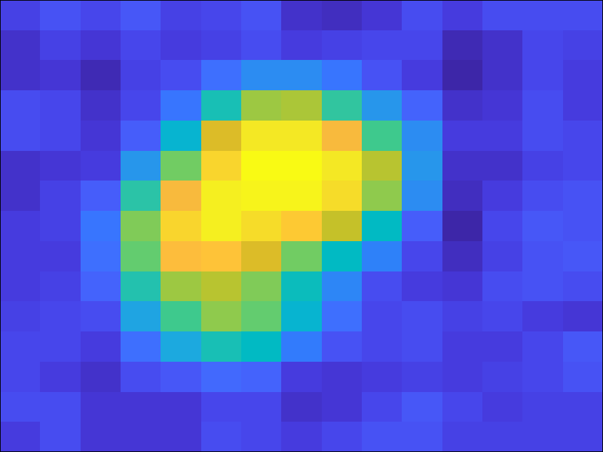
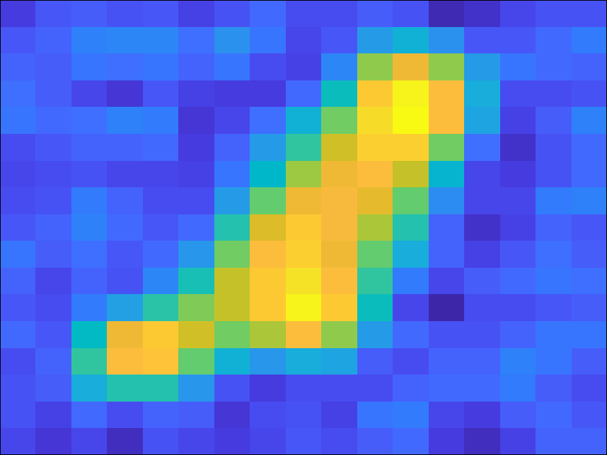
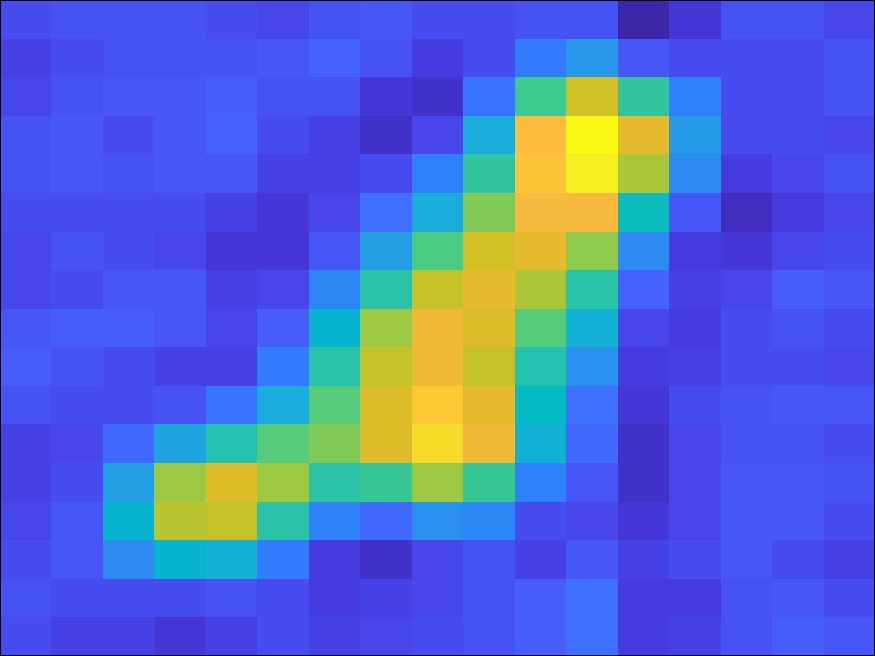
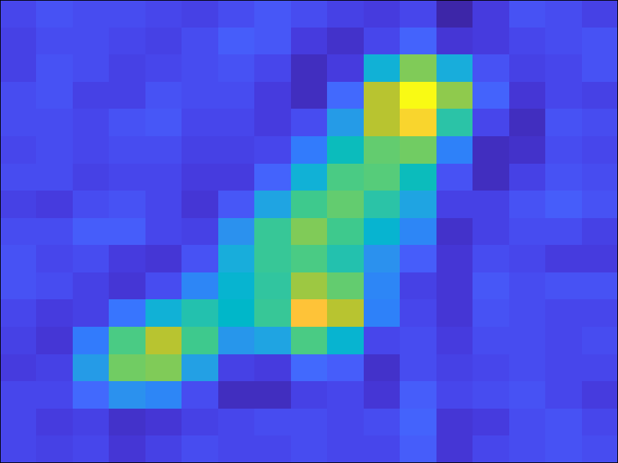
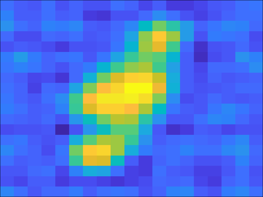
(a) Ours_Sep

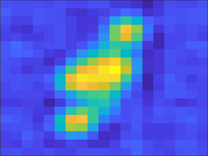
(b) Ours_Joint

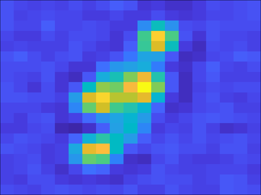
(c) Ours_Alter

(d) GT

Figure 7: The estimated four kind of kernels by different optimization manners, where the last column are Ground Truth (GT) and the first three columns are the results from Ours_Alter, Ours_Joint and Ours_Sep, respectively.

Ours_Sep

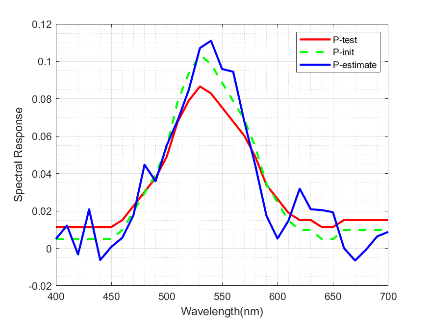
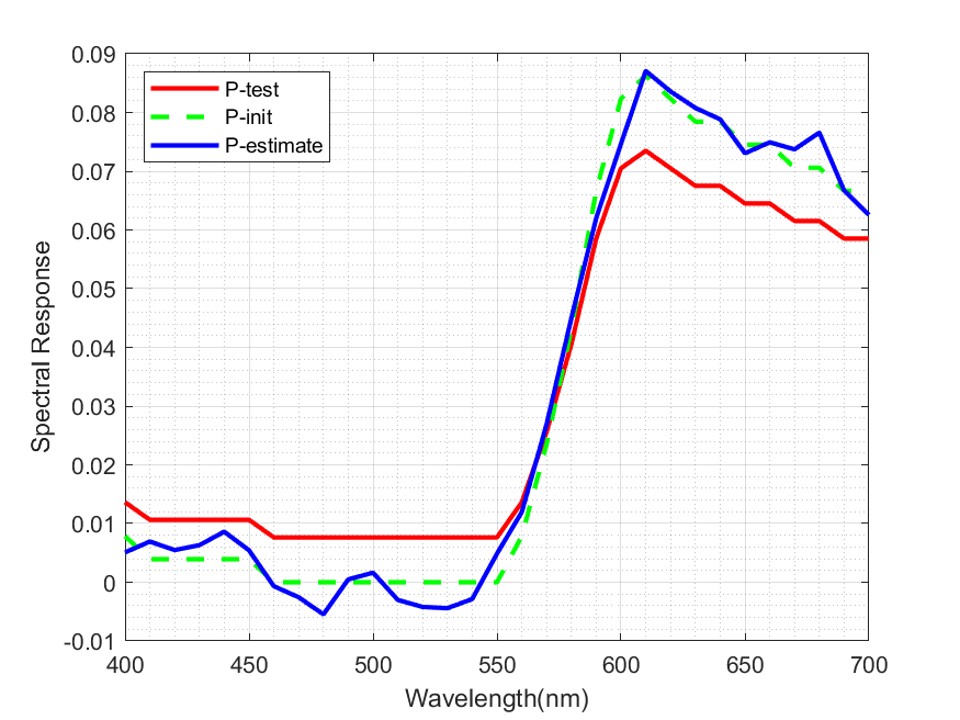
Ours_Joint

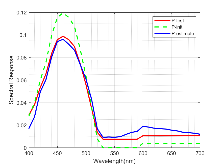
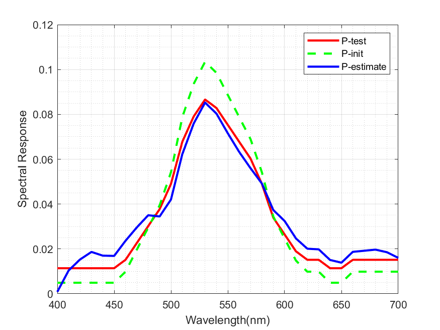
Ours_Alter

(a) Blue band

(b) Green band

(c) Red band

Figure 8: The estimated spectral response matrices by different optimization manners, from the top row to the bottom are Ours_Sep, Ours_Joint and Ours_Alter, respectively.

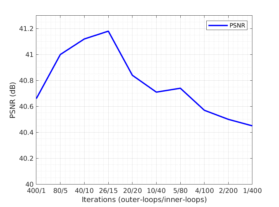
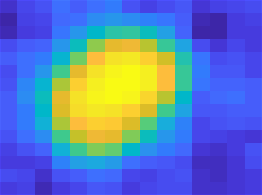
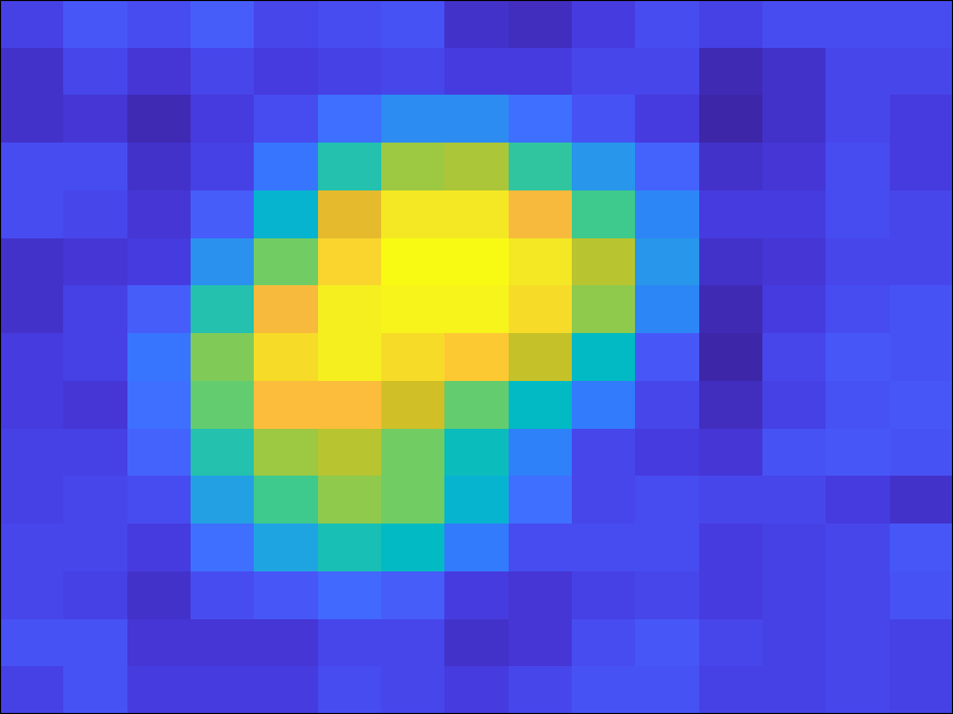
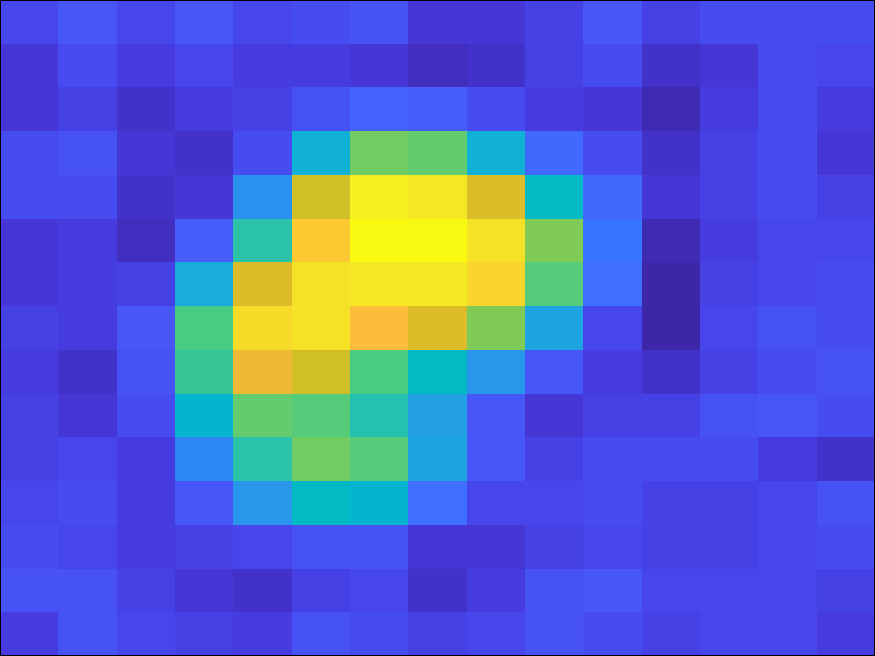
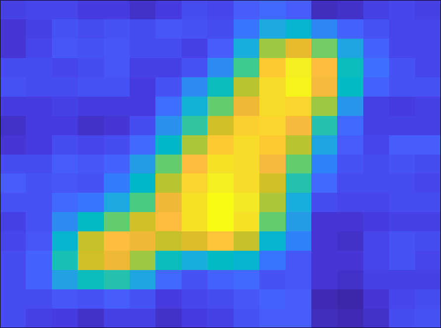
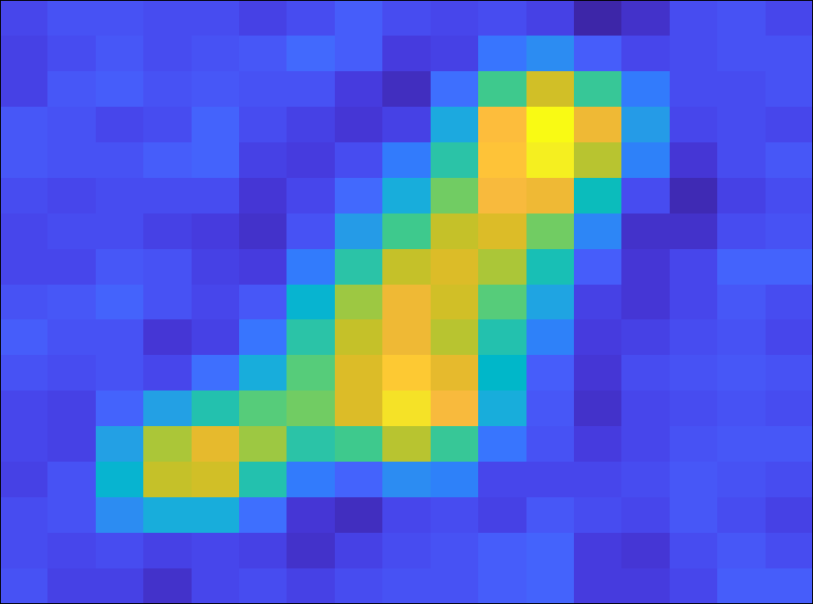
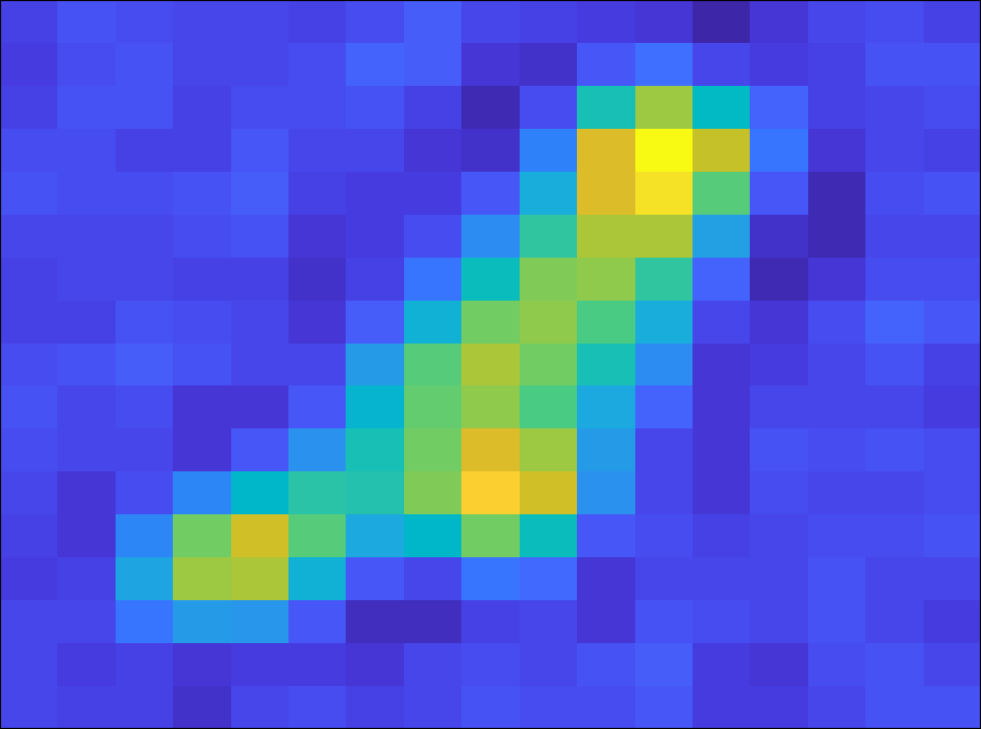
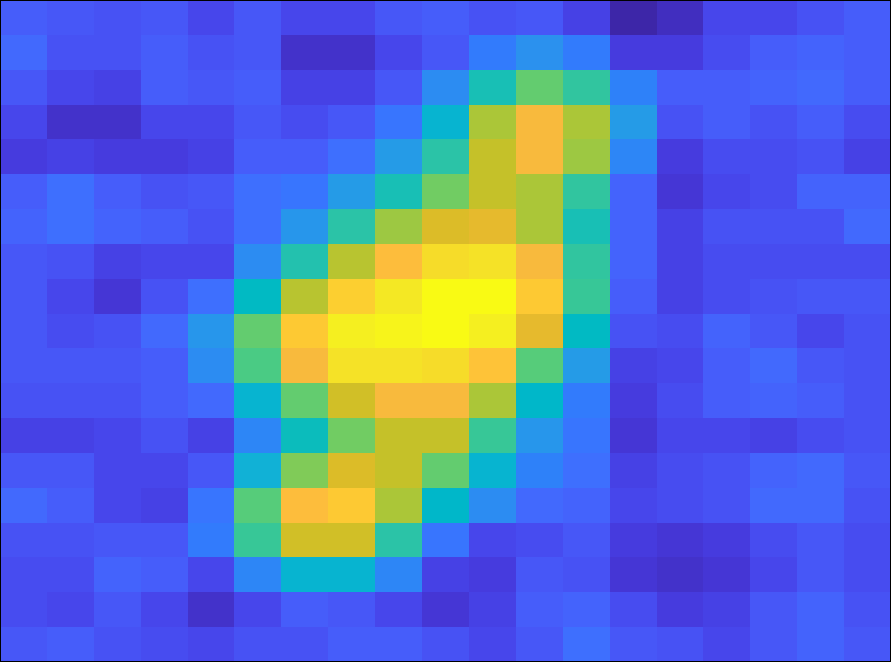
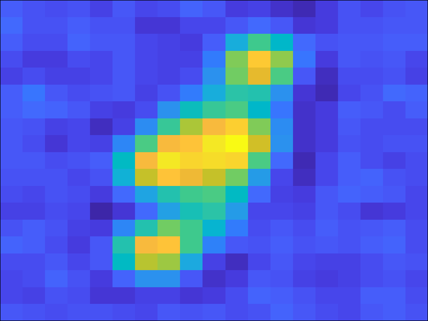
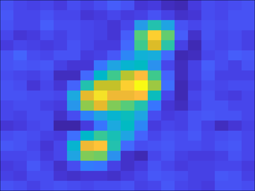
Effect of different iteration numbers The proposed method is implemented by iteratively alternating optimization strategy, which is consisted by an outer-loop iteration and an inner-loop iteration. $I_{out}$ denotes the number of conducting alternating optimization (outer-loop) and $I_{in}$ indicates the independent optimization for the estimation and reconstruction networks (inner-loop). In this experiment, we fix the total iteration number $I$ as 400 ($I=I_{out}\times I_{in}$). Thus, the increase of $I_{out}$ will decrease the correspondingly $I_{in}$, and vice versa. Therefore, in our experiment, we only verify the influence of changing $I_{out}$, which is directly related with alternating optimization. In experiment, we conduct the experiments on the CAVE dataset with different $I_{out}$. SNRs of both the observed LR HSI and HR MSI are 40dB and the SR scale is 8. The blur kernels and the spectral response matrix for the test data is $\mathbf{k}_{1}$ with $\mathbf{P}_{0.01}$, respectively. The experimental results are plotted in Figure 9. It can be seen a large $I_{out}$ often presents a better PSNR result, which demonstrates that the increase of time on alternation optimization is benefit to improve the performance of blind HSI fusion SR. Thus, in all experiments, we empirically set the number of $I_{out}$ is 40.

Figure 9: The variations of PSNR when changing the iteration numbers of outer-loop and inner-loop.

(a) GT

(b) $I_{out}$ = 10

(c) $I_{out}$ = 20

(d) $I_{out}$ = 30

(e) $I_{out}$ = 40

Figure 10: The estimated kernels by the proposed method with different iteration numbers.

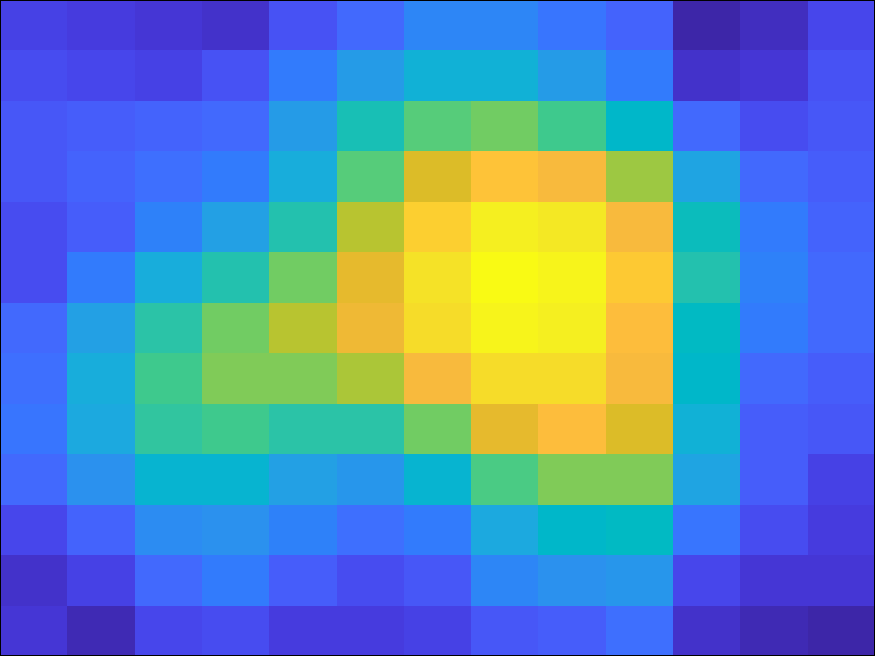
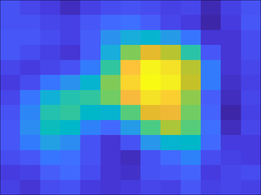
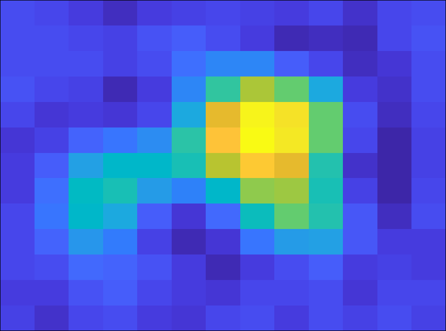
In the experiments corresponding to Figure 7 and Figure 8, we have demonstrated the proposed method can well estimate the degeneration models. In this experiment, we further visualize the intermediate results (the estimated kernels in the intermediate stages) of the reconstructed blur kernel with different iteration number of alternating optimization. We conduct the experiments on different four kind of motion kernels with $\mathbf{P}_{0.01}$ as the test spectral response matrix. SNRs of both the observed LR HSI and HR MSI are 40dB, and the SR scale is 8. The estimated kernels with different iteration numbers are shown in Figure 10. It can be seen that the estimation of blur kernels can be gradually improved with more iteration numbers, which also results in better performance of reconstruction network accordingly.

7.2 More experimental results on the benchmark datasets

Table 8: The performance of each method on the CAVE dataset with input images, which suffers from noise with different intensities. The best results are in bold.

Noise intensity	Method	RMSE	PSNR	SAM	SSIM
HSI 40dB MSI 40dB	NSSR [5]	8.11	30.53	18.85	0.8533
	MHFnet [23]	4.53	35.67	14.01	0.9409
	Yong [13]	4.46	35.72	11.29	0.9491
	UAL [31]	3.93	37.07	7.57	0.9724
	DBSR [30]	4.01	36.66	5.53	0.9739
	Ours	2.40	41.12	6.53	0.9854
HSI 35dB MSI 35dB	NSSR [5]	8.95	29.52	26.27	0.7462
	MHFnet [23]	4.85	34.91	18.40	0.9040
	Yong [13]	4.58	35.48	12.70	0.9415
	UAL [31]	4.09	36.57	9.70	0.9652
	DBSR [30]	4.61	35.56	7.74	0.9624
	Ours	2.67	40.21	8.74	0.9797
HSI 30dB MSI 30dB	NSSR [5]	11.16	27.40	35.34	0.5623
	MHFnet [23]	5.69	33.30	24.54	0.8279
	Yong [13]	4.87	34.82	14.92	0.9244
	UAL [31]	4.45	35.70	13.17	0.9495
	DBSR [30]	6.15	32.97	12.49	0.9243
	Ours	3.20	38.36	12.45	0.9632

(a) GT

(b) NSSR [5]

(c) MHFnet [23]

(d) Yong [13]

(e) UAL [31]

(f) DBSR [30]

(g) Ours

Figure 11: The visual SR results of all methods on the CAVE dataset. The observed LR HSI and HR MSI generated by $\mathbf{k}_{1}$ and $\mathbf{P}_{0.01}$, respectively. SNRs of both two observed images are 40dB, and the SR scale is 8.

(a) GT

(b) NSSR [5]

(c) MHFnet [23]

(d) Yong [13]

(e) UAL [31]

(f) DBSR [30]

(g) Ours

Figure 12: The visual SR results of all methods on the Harvard dataset. The observed LR HSI and HR MSI generated by $\mathbf{k}_{1}$ and $\mathbf{P}_{0.01}$, respectively. SNRs of both two observed images are 40dB, and the SR scale is 16.

The experiment results on the CAVE dataset In the main manuscript, we have demonstrated several experimental results on the CAVE dataset with different settings. In this experiment, considering the observed images are always contaminated by noise, we further verify the performance of the proposed method influenced by the observed images with noise. For this purpose, we add the noise with different intensities into the original noisy-free images, which results in the observed images different SNRs. In experiment, the test LR HSI and HR MSI are generated from $\mathbf{k}_{1}$ and $\mathbf{P}_{0.01}$, respectively, and the SR scale is 8. We summarize the corresponding numerical results in Table 8. It can be seen that the performance of all methods degrade with larger noise intensity. For example, the SAM of NSSR [5] decreases to 35 when the SNR is 30dB. Nevertheless, the results of Ours still obtain obvious advantages over the competing four evaluation metrics.

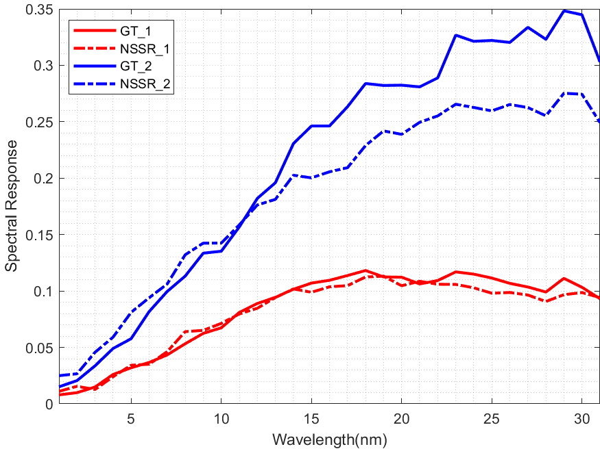
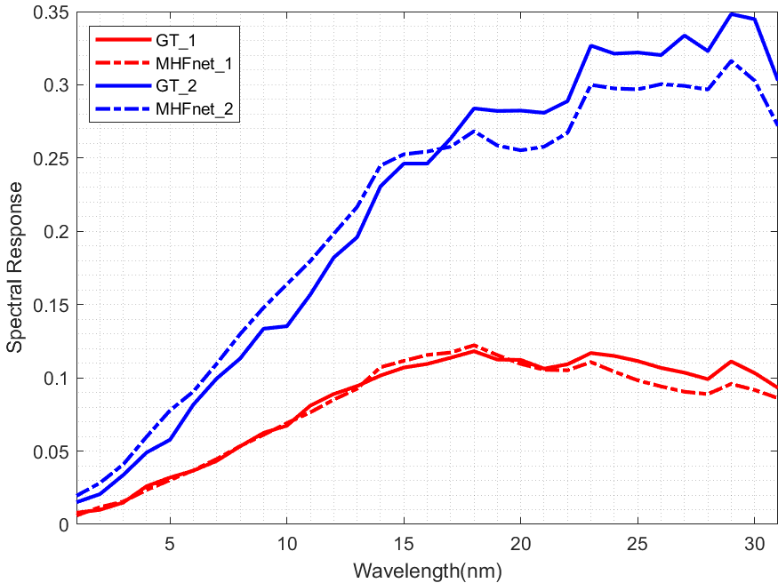
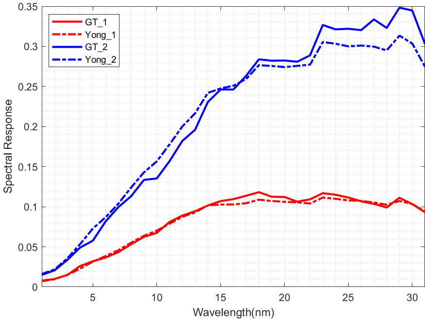
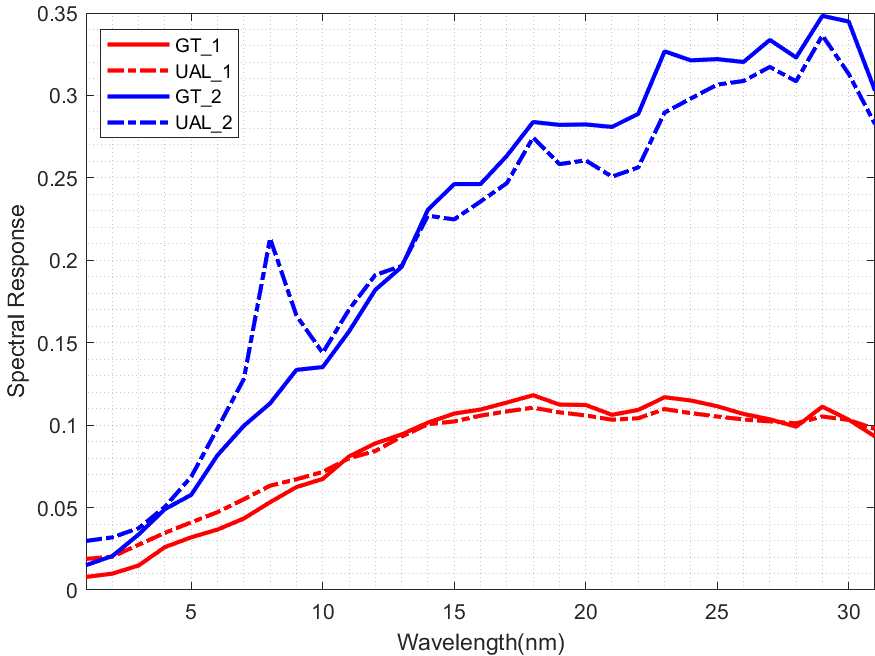
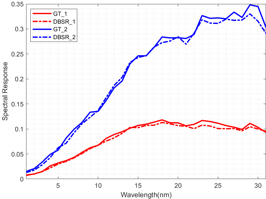
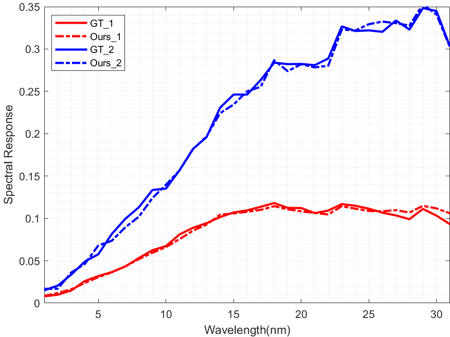
In addition, to further clarify the superiority of the proposed method, we select two representative pixels (marked by different colors) in the displayed HSI to plot the reconstructed spectral curve. The corresponding spectral curves are provided in the third row of Figure 11, in which the reconstructed spectrum is plotted with a dotted line and the ground truth spectrum is plotted with a solid line. It can be seen that the proposed method can accurately reconstructs the spectra, which demonstrates it has smaller spectral distortion compared than the competing methods.

The experiment results on the Harvard dataset In this experiment, we give the visual SR results and the reconstruction curves of spectra in Figure 12. It can be seen that the reconstructed results of the proposed method have more details and lower reconstruction errors than the competing methods. In addition, the reconstructed spectrum of the proposed method is much closer to the ground truth than the other methods. From above experimental results, we can conclude the proposed blind HSI SR method can well reconstruct the latent HSI in both spatial and spectral domain on the Harvard dataset.

Table 9: The performance of each method on the NTIRE dataset with different SR scale factors, while the input LR HSI and HR MSI generated by $\mathbf{k}_{1}$ and $\mathbf{P}_{0.01}$, respectively. The SNR of this two input images are both 40dB, and the best results are in bold.

Methods	s = 8				s = 16				s = 32
	RMSE	PSNR	SAM	SSIM	RMSE	PSNR	SAM	SSIM	RMSE	PSNR	SAM	SSIM
NSSR [5]	7.11	31.43	1.55	0.9447	6.69	32.01	2.46	0.9454	5.91	33.09	2.81	0.9696
MHFnet [23]	3.16	38.78	1.53	0.9928	3.44	38.07	1.69	0.9925	4.06	36.58	2.14	0.9920
Yong [13]	3.27	38.23	1.57	0.9804	4.19	36.23	2.11	0.9774	4.51	35.59	2.50	0.9801
UAL [31]	4.68	35.61	2.21	0.9924	5.61	33.64	2.27	0.9891	6.05	32.97	2.27	0.9864
DBSR [30]	7.08	33.10	0.73	0.9799	6.61	33.47	0.95	0.9788	11.43	27.85	1.54	0.9542
Ours	2.19	41.75	0.88	0.9955	2.31	41.28	1.09	0.9951	3.11	38.69	1.46	0.9936

(a) GT

(b) NSSR [5]

(c) MHFnet [23]

(d) Yong [13]

(e) UAL [31]

(f) DBSR [30]

(g) Ours

Figure 13: The visual SR results of all methods on the ICLV dataset. The observed LR HSI and HR MSI generated by $\mathbf{k}_{1}$ and $\mathbf{P}_{0.01}$, respectively. SNRs of both two observed images are 40dB, and the SR scale is 32.

The experiment results on the NTIRE dataset In this experiment, we further compare the proposed method with the other competing methods on the NTIRE dataset with different SR scales. The observed LR HSI and HR MSI are generated by $\mathbf{k}_{1}$ and $\mathbf{P}_{0.01}$, respectively. SNRs of both these two observed images are 40dB. We summarize the detailed numerical results in the Table 9. Same as the results on the CAVE and Harvard datasets, the proposed method also has obvious advantage over the other comparison methods. In addition, we also provides the visual results of all methods for further comparison. In Figure 13, the visual results of the reconstructed HSI and the corresponding spectrum curve are provided. It can be seen that the proposed method obtains better performance than the other comparison methods. The proposed method can well reconstruct the latent HSI in both the spatial and the spectral domains.

References

- [1] S. Bernabé, C. García, F. D. Igual, G. Botella, M. Prieto-Matias, and A. Plaza. Portability study of an opencl algorithm for automatic target detection in hyperspectral images. IEEE Transactions on Geoscience and Remote Sensing, 57(11):9499–9511, 2019.
- [2] J. Cai, H. Zeng, H. Yong, Z. Cao, and L. Zhang. Toward real-world single image super-resolution: A new benchmark and a new model. In 2019 IEEE/CVF International Conference on Computer Vision (ICCV), pages 3086–3095, 2019.
- [3] A. Chakrabarti and T. Zickler. Statistics of real-world hyperspectral images. In CVPR 2011, pages 193–200, 2011.
- [4] R. Dian, L. Fang, and S. Li. Hyperspectral image super-resolution via non-local sparse tensor factorization. In 2017 IEEE Conference on Computer Vision and Pattern Recognition (CVPR), pages 3862–3871, 2017.
- [5] W. Dong, F. Fu, G. Shi, X. Cao, J. Wu, G. Li, and X. Li. Hyperspectral image super-resolution via non-negative structured sparse representation. IEEE Transactions on Image Processing, 25(5):2337–2352, 2016.
- [6] Chelsea Finn, Pieter Abbeel, and Sergey Levine. Model-agnostic meta-learning for fast adaptation of deep networks. In Proceedings of the 34th International Conference on Machine Learning - Volume 70, Aug 2017.
- [7] J. Gu, H. Lu, W. Zuo, and C. Dong. Blind super-resolution with iterative kernel correction. In 2019 IEEE/CVF Conference on Computer Vision and Pattern Recognition (CVPR), pages 1604–1613, 2019.
- [8] N. He, M. E. Paoletti, J. M. Haut, L. Fang, S. Li, A. Plaza, and J. Plaza. Feature extraction with multiscale covariance maps for hyperspectral image classification. IEEE Transactions on Geoscience and Remote Sensing, 57(2):755–769, 2019.
- [9] S. A. Hussein, T. Tirer, and R. Giryes. Correction filter for single image super-resolution: Robustifying off-the-shelf deep super-resolvers. In 2020 IEEE/CVF Conference on Computer Vision and Pattern Recognition (CVPR), pages 1425–1434, 2020.
- [10] S. Jia, Z. Lin, B. Deng, J. Zhu, and Q. Li. Cascade superpixel regularized gabor feature fusion for hyperspectral image classification. IEEE Transactions on Neural Networks and Learning Systems, 31(5):1638–1652, 2020.
- [11] Diederik Kingma and Jimmy Ba. Adam: A method for stochastic optimization. Computer Science, pages 0–0, 2014.
- [12] V. Lempitsky, A. Vedaldi, and D. Ulyanov. Deep image prior. In 2018 IEEE/CVF Conference on Computer Vision and Pattern Recognition, pages 9446–9454, 2018.
- [13] Y. Li, L. Zhang, C. Tian, C. Ding, Y. Zhang, and W. Wei. Hyperspectral image super-resolution extending: An effective fusion based method without knowing the spatial transformation matrix. In 2017 IEEE International Conference on Multimedia and Expo (ICME), pages 1117–1122, 2017.
- [14] Zhengxiong Luo, Y. Huang, Shang Li, Liang Wang, and Tieniu Tan. Unfolding the alternating optimization for blind super resolution. ArXiv, abs/2010.02631, 2020.
- [15] Jiangtao Nie, Lei Zhang, Cong Wang, Wei Wei, and Yanning Zhang. Robust deep hyperspectral imagery super-resolution. In IGARSS 2019 IEEE International Geoscience and Remote Sensing Symposium, pages 847–850, July 2019.
- [16] Adam Paszke, Sam Gross, Francisco Massa, Adam Lerer, and James Bradbury. Pytorch: An imperative style, high-performance deep learning library. In Advances in Neural Information Processing Systems 32, pages 8024–8035. 2019.
- [17] Ying Qu, Hairong Qi, and Chiman Kwan. Unsupervised sparse dirichlet-net for hyperspectral image super-resolution. Proceedings of the IEEE Conference on Computer Vision and Pattern Recognition, pages 2511–2520, 2018.
- [18] J. W. Soh, S. Cho, and N. I. Cho. Meta-transfer learning for zero-shot super-resolution. In 2020 IEEE/CVF Conference on Computer Vision and Pattern Recognition (CVPR), pages 3513–3522, 2020.
- [19] B. Uzkent, A. Rangnekar, and M. J. Hoffman. Tracking in aerial hyperspectral videos using deep kernelized correlation filters. IEEE Transactions on Geoscience and Remote Sensing, 57(1):449–461, 2019.
- [20] W. Wang, W. Zeng, Y. Huang, X. Ding, and J. Paisley. Deep blind hyperspectral image fusion. In 2019 IEEE/CVF International Conference on Computer Vision (ICCV), pages 4149–4158, 2019.
- [21] W. Wenzheng, Z. Baojun, T. Linbo, Z. Shichao, and F. Fan. Fusion-based spectral matching method for hyperspectral target detection. The Journal of Engineering, 2019(20):6741–6744, 2019.
- [22] R. Wu, W. Ma, X. Fu, and Q. Li. Hyperspectral super-resolution via global-local low-rank matrix estimation. IEEE Transactions on Geoscience and Remote Sensing, pages 1–16, 2020.
- [23] Q. Xie, M. Zhou, Q. Zhao, D. Meng, W. Zuo, and Z. Xu. Multispectral and hyperspectral image fusion by ms/hs fusion net. In 2019 IEEE/CVF Conference on Computer Vision and Pattern Recognition (CVPR), pages 1585–1594, 2019.
- [24] F. Xiong, J. Zhou, and Y. Qian. Material based object tracking in hyperspectral videos. IEEE Transactions on Image Processing, 29:3719–3733, 2020.
- [25] Jingxiang Yang, Yongqiang Zhao, Chen Yi, and Jonathan Cheung-Wai Chan. No-reference hyperspectral image quality assessment via quality-sensitive features learning. Remote Sensing, 9(4), 2017.
- [26] Jingxiang Yang, Yong-Qiang Zhao, and Jonathan Cheung-Wai Chan. Hyperspectral and multispectral image fusion via deep two-branches convolutional neural network. Remote Sensing, 10(5), 2018.
- [27] F. Yasuma, T. Mitsunaga, D. Iso, and S. K. Nayar. Generalized assorted pixel camera: Postcapture control of resolution, dynamic range, and spectrum. IEEE Transactions on Image Processing, 19(9):2241–2253, 2010.
- [28] K. Zhang, W. Zuo, and L. Zhang. Learning a single convolutional super-resolution network for multiple degradations. In 2018 IEEE/CVF Conference on Computer Vision and Pattern Recognition, pages 3262–3271, 2018.
- [29] K. Zhang, W. Zuo, and L. Zhang. Deep plug-and-play super-resolution for arbitrary blur kernels. In 2019 IEEE/CVF Conference on Computer Vision and Pattern Recognition (CVPR), pages 1671–1681, 2019.
- [30] L. Zhang, J. Nie, W. Wei, Y. Li, and Y. Zhang. Deep blind hyperspectral image super-resolution. IEEE Transactions on Neural Networks and Learning Systems, pages 1–13, 2020.
- [31] Lei Zhang, Jiangtao Nie, Wei Wei, Yanning Zhang, Shengcai Liao, and Ling Shao. Unsupervised adaptation learning for hyperspectral imagery super-resolution. In IEEE/CVF Conference on Computer Vision and Pattern Recognition (CVPR), June 2020.
- [32] L. Zhang, W. Wei, C. Bai, Y. Gao, and Y. Zhang. Exploiting clustering manifold structure for hyperspectral imagery super-resolution. IEEE Transactions on Image Processing, 27(12):5969–5982, 2018.
- [33] R. Zhou and S. Süsstrunk. Kernel modeling super-resolution on real low-resolution images. In 2019 IEEE/CVF International Conference on Computer Vision (ICCV), pages 2433–2443, 2019.