Lower Bounds for Semialgebraic Range Searching and Stabbing Problems

Peyman Afshani peyman@cs.au.dk ย andย  Pingan Cheng pingancheng@cs.au.dk Aarhus UniversityAarhusDenmark
Abstract.

In the semialgebraic range searching problem, we are given a set of n๐‘›n points in โ„dsuperscriptโ„๐‘‘\mathbb{R}^{d} and we want to preprocess the points such that for any query range belonging to a family of constant complexity semialgebraic sets (Tarski cells), all the points intersecting the range can be reported or counted efficiently. When the ranges are composed of simplices, then the problem is well-understood: it can be solved using Sโ€‹(n)๐‘†๐‘›S(n) space and with Qโ€‹(n)๐‘„๐‘›Q(n) query time with Sโ€‹(n)โ€‹Qโ€‹(n)d=O~โ€‹(nd)๐‘†๐‘›๐‘„superscript๐‘›๐‘‘~๐‘‚superscript๐‘›๐‘‘S(n)Q(n)^{d}=\tilde{O}(n^{d}) where the O~โ€‹(โ‹…)~๐‘‚โ‹…\tilde{O}(\cdot) notation hides polylogarithmic factors and this trade-off is tight (up to noโ€‹(1)superscript๐‘›๐‘œ1n^{o(1)} factors). Consequently, there exists โ€œlow spaceโ€ structures that use Oโ€‹(n)๐‘‚๐‘›O(n) space with Oโ€‹(n1โˆ’1/d)๐‘‚superscript๐‘›11๐‘‘O(n^{1-1/d}) query time and โ€œfast queryโ€ structures that use Oโ€‹(nd)๐‘‚superscript๐‘›๐‘‘O(n^{d}) space with Oโ€‹(logd+1โกn)๐‘‚superscript๐‘‘1๐‘›O(\log^{d+1}n) query time. However, for the general semialgebraic ranges, only โ€œlow spaceโ€ solutions are known, but the best solutions match the same trade-off curve as the simplex queries, with Oโ€‹(n)๐‘‚๐‘›O(n) space and O~โ€‹(n1โˆ’1/d)~๐‘‚superscript๐‘›11๐‘‘\tilde{O}(n^{1-1/d}) query time. It has been conjectured that the same could be done for the โ€œfast queryโ€ case but this open problem has stayed unresolved.

Here, we disprove this conjecture. We give the first nontrivial lower bounds for semilagebraic range searching and other related problems. More precisely, we show that any data structure for reporting the points between two concentric circles, a problem that we call 2D annulus reporting problem, with Qโ€‹(n)๐‘„๐‘›Q(n) query time must use Sโ€‹(n)=ฮฉ๐‘œโ€‹(n3/Qโ€‹(n)5)๐‘†๐‘›๐‘œฮฉsuperscript๐‘›3๐‘„superscript๐‘›5S(n)=\overset{\scriptscriptstyle o}{\Omega}(n^{3}/Q(n)^{5}) space where the ฮฉ๐‘œโ€‹(โ‹…)๐‘œฮฉโ‹…\overset{\scriptscriptstyle o}{\Omega}(\cdot) notation hides noโ€‹(1)superscript๐‘›๐‘œ1n^{o(1)} factors, meaning, for Qโ€‹(n)=logOโ€‹(1)โกn๐‘„๐‘›superscript๐‘‚1๐‘›Q(n)=\log^{O(1)}n, ฮฉ๐‘œโ€‹(n3)๐‘œฮฉsuperscript๐‘›3\overset{\scriptscriptstyle o}{\Omega}(n^{3}) space must be used. In addition, we study the problem of reporting the subset of input points between two polynomials of the form Y=โˆ‘i=0ฮ”aiโ€‹Xi๐‘Œsuperscriptsubscript๐‘–0ฮ”subscript๐‘Ž๐‘–superscript๐‘‹๐‘–Y=\sum_{i=0}^{\Delta}a_{i}X^{i} where values a0,โ‹ฏ,aฮ”subscript๐‘Ž0โ‹ฏsubscript๐‘Žฮ”a_{0},\cdots,a_{\Delta} are given at the query time, a problem that we call polynomial slab reporting. For this, we show a space lower bound of ฮฉ๐‘œโ€‹(nฮ”+1/Qโ€‹(n)(ฮ”+3)โ€‹ฮ”/2)๐‘œฮฉsuperscript๐‘›ฮ”1๐‘„superscript๐‘›ฮ”3ฮ”2\overset{\scriptscriptstyle o}{\Omega}(n^{\Delta+1}/Q(n)^{(\Delta+3)\Delta/2}), which shows for Qโ€‹(n)=logOโ€‹(1)โกn๐‘„๐‘›superscript๐‘‚1๐‘›Q(n)=\log^{O(1)}n, we must use ฮฉ๐‘œโ€‹(nฮ”+1)๐‘œฮฉsuperscript๐‘›ฮ”1\overset{\scriptscriptstyle o}{\Omega}(n^{\Delta+1}) space. We also consider the dual problems of semialgebraic range searching, semialgebraic stabbing problems, and present lower bounds for them. In particular, we show that in linear space, any data structure that solves 2D annulus stabbing problems must use ฮฉโ€‹(n2/3)ฮฉsuperscript๐‘›23\Omega(n^{2/3}) query time. Note that this almost matches the upper bound obtained by lifting 2D annuli to 3D. Like semialgebraic range searching, we also present lower bounds for general semialgebraic slab stabbing problems. Again, our lower bounds are almost tight for linear size data structures in this case.

Semialgebraic Range Searching, Lower Bound, Computational Geometry
Supported by DFF (Det Frie Forskningsrรฅd) of Danish Council for Independent Research under grant ID DFFโˆ’-7014โˆ’-00404.
โ€ โ€ copyright: acmcopyrightโ€ โ€ booktitle: โ€ โ€ ccs: Theory of computationย Computational geometry

1. Introduction

We address one of the biggest open problems of the recent years in the range searching area. Our main results are lower bounds in the pointer machine model of computation that essentially show that the so-called โ€œfast queryโ€ version of the semialgebraic range reporting problem is โ€œimperviousโ€ to the algebraic techniques. Our main result reveals that to obtain polylogarithmic query time, the data structure requires ฮฉ๐‘œโ€‹(nฮ”+1)๐‘œฮฉsuperscript๐‘›ฮ”1\overset{\scriptscriptstyle o}{\Omega}(n^{\Delta+1}) space111 ฮฉ๐‘œโ€‹(โ‹…)๐‘œฮฉโ‹…\overset{\scriptscriptstyle o}{\Omega}(\cdot), O๐‘œโ€‹(โ‹…)๐‘œ๐‘‚โ‹…\overset{\scriptscriptstyle o}{O}(\cdot), ฮ˜๐‘œโ€‹(โ‹…)๐‘œฮ˜โ‹…\overset{\scriptscriptstyle o}{\Theta}(\cdot) notations hide noโ€‹(1)superscript๐‘›๐‘œ1n^{o(1)} factors and ฮฉ~โ€‹(โ‹…)~ฮฉโ‹…\tilde{\Omega}(\cdot), O~โ€‹(โ‹…)~๐‘‚โ‹…\tilde{O}(\cdot), ฮ˜~โ€‹(โ‹…)~ฮ˜โ‹…\tilde{\Theta}(\cdot) notations hide logOโ€‹(1)โกnsuperscript๐‘‚1๐‘›\log^{O(1)}n factors., where the constant depends on ฮ”ฮ”\Delta, n๐‘›n is the input size, and ฮ”+1ฮ”1\Delta+1 is the number of parameters of each โ€œpolynomial inequalityโ€ (these will be defined more clearly later). Thus, we refute a relatively popular recent conjecture that data structures with O๐‘œโ€‹(nd)๐‘œ๐‘‚superscript๐‘›๐‘‘\overset{\scriptscriptstyle o}{O}(n^{d}) space and polylogarithmic query time could exist, where d๐‘‘d is the dimension of the input points. Surprisingly, the proofs behind these lower bounds are simple, and these lower bounds could have been discovered years ago as the tools we use already existed decades ago.

Range searching is a broad area of research in which we are given a set P๐‘ƒP of n๐‘›n points in โ„dsuperscriptโ„๐‘‘\mathbb{R}^{d} and the goal is to preprocess P๐‘ƒP such that given a query range โ„›โ„›\mathscr{R}, we can count or report the subset of P๐‘ƒP that lies in โ„›โ„›\mathscr{R}. Often โ„›โ„›\mathscr{R} is restricted to a fixed family of ranges, e.g., in simplex range counting problem, โ„›โ„›\mathscr{R} is a simplex in โ„dsuperscriptโ„๐‘‘\mathbb{R}^{d} and the goal is to report |Pโˆฉโ„›|๐‘ƒโ„›|P\cap\mathscr{R}|, or in halfspace range reporting problem, โ„›โ„›\mathscr{R} is a halfspace and the goal is to report Pโˆฉโ„›๐‘ƒโ„›P\cap\mathscr{R}. Range searching problems have been studied extensively and they have numerous variants. For an overview of this topic, we refer the readers to an excellent survey by Agarwalย (Goodman etย al., 2018).

Another highly related problem which can be viewed as the โ€œdualโ€ of this problem is range stabbing: we are given a set R๐‘…R of ranges as input and the goal is to preprocess R๐‘…R such that given a query point p๐‘p, we can count or report the ranges of R๐‘…R containing p๐‘p efficiently. Here, we focus on the reporting version of range stabbing problems.

1.1. Range Searching: A Very Brief Survey

1.1.1. Simplex Range Searching

Simplices is one of the most fundamental family of queries. In fact, if the query is decomposable (such as range counting or range reporting queries), then simplices can be used as โ€œbuilding blocksโ€ to answer more complicated queries: for a query โ„›โ„›\mathscr{R} which is a polyhedral region of Oโ€‹(1)๐‘‚1O(1) complexity, we can decompose it into Oโ€‹(1)๐‘‚1O(1) disjoint simplices (with a constant that depends on d๐‘‘d) and thus answering โ„›โ„›\mathscr{R} can be reduced to answering Oโ€‹(1)๐‘‚1O(1) simplicial queries.

Simplicial queries were hotly investigated in 1980s and this led to development of two important tools in computational geometry: cuttings and partition theorem and both of them have found applications in areas not related to range searching.

Cuttings and Fast Data Structures

โ€œFast queryโ€ data structures can answer simplex range counting or reporting queries in polylogarithmic query time but by using Oโ€‹(nd)๐‘‚superscript๐‘›๐‘‘O(n^{d}) space and they can be built using cuttings. In a nut-shell, given a set H๐ปH of n๐‘›n hyperplanes in โ„dsuperscriptโ„๐‘‘\mathbb{R}^{d}, a 1r1๐‘Ÿ\frac{1}{r}-cutting, is a decomposition of โ„dsuperscriptโ„๐‘‘\mathbb{R}^{d} into Oโ€‹(rd)๐‘‚superscript๐‘Ÿ๐‘‘O(r^{d}) simplices such that each simplex is intersected by Oโ€‹(n/r)๐‘‚๐‘›๐‘ŸO(n/r) hyperplanes of H๐ปH. These were developed by some of the pioneers in the range searching area, such as Clarksonย (Clarkson, 1987), Haussler and Welzlย (Haussler and Welzl, 1986), Chazelle and Friedmanย (Chazelle and Friedman, 1990), Matouลกekย (Matouลกek, 1991), finally culminating in a result of Chazelleย (Chazelle, 1993) who optimized various aspects of cuttings. Using cuttings, one can answer simplex range counting, or reporting queries with Oโ€‹(nd)๐‘‚superscript๐‘›๐‘‘O(n^{d}) space and Oโ€‹((logโกn)d+1+k)๐‘‚superscript๐‘›๐‘‘1๐‘˜O((\log n)^{d+1}+k) query time (where k๐‘˜k is the output size)ย (Matouลกek, 1993). The query time can be lowered to Oโ€‹(logโกn)๐‘‚๐‘›O(\log n) by increasing the space slightly to Oโ€‹(nd+ฮต)๐‘‚superscript๐‘›๐‘‘๐œ€O(n^{d+\varepsilon}) for any constant ฮต>0๐œ€0\varepsilon>0ย (Chazelle and Welzl, 1989). An interested reader can refer to a survey on cuttings by Chazelleย (Chazelle, 2018).

The Partition Theorem and Space-efficient Data Structures

At the opposite end of the spectrum, simplex range counting or reporting queries can be answered using linear space but with higher query time of Oโ€‹(n1โˆ’1/d)๐‘‚superscript๐‘›11๐‘‘O(n^{1-1/d}), using partition trees and the related techniques. This branch of techniques has a very interesting history. In 1982, Willardย (Willard, 1982) cleverly used ham sandwich theorem to obtain a linear-sized data structure with query time of Oโ€‹(nฮณ)๐‘‚superscript๐‘›๐›พO(n^{\gamma}) for some constant ฮณ<1๐›พ1\gamma<1 for simplicial queries in 2D. After a number of attempts that either improved the exponent or generalized the technique to higher dimensions, Welzlย (Welzl, 1988) in 1982 provided the first optimal exponent for the partition trees, then Chazelle et al.ย (Chazelle and Welzl, 1989) provided the first near-linear size data structure with query time of roughly Oโ€‹(n1โˆ’1/d)๐‘‚superscript๐‘›11๐‘‘O(n^{1-1/d}). Finally, a data structure with Oโ€‹(n)๐‘‚๐‘›O(n) space and Oโ€‹(n1โˆ’1/d)๐‘‚superscript๐‘›11๐‘‘O(n^{1-1/d}) query time was given by Matouลกekย (Matouลกek, 1993). This was also simplified recently by Chanย (Chan, 2012).

Space/Query Time Trade-off

It is possible to combine fast query data structures and linear-sized data structures to solve simplex queries with Sโ€‹(n)๐‘†๐‘›S(n) space and Qโ€‹(n)๐‘„๐‘›Q(n) query time such that Sโ€‹(n)โ€‹Qโ€‹(n)d=O~โ€‹(nd)๐‘†๐‘›๐‘„superscript๐‘›๐‘‘~๐‘‚superscript๐‘›๐‘‘S(n)Q(n)^{d}=\tilde{O}(n^{d}). This trade-off between space and query time is optimal, at least in the pointer machine model and in the semigroup modelย (Afshani, 2012; Chazelle and Rosenberg, 1996; Chazelle, 1989).

Multi-level Structures, Stabbing and Other Related Queries

By using multi-level data structures, one can solve more complicated problems where both the input and the query shapes can be simplicial objects of constant complexity. The best multi-level data structures use one extra logโกn๐‘›\log n factor in space and query time per levelย (Chan, 2012) and there exist lower bounds that show space/query time trade-off should blow up by at least logโกn๐‘›\log n factor per levelย (Afshani and Driemel, 2018). This means that problems such as simplex stabbing (where the input is a set of simplices and we want to output the simplices containing a given query point) or simplex-simplex containment problem (where the input is a set of simplices, and we want to output simplices fully contained in a query simplex) all have the same trade-off curve of Sโ€‹(n)โ€‹Qโ€‹(n)d=O~โ€‹(nd)๐‘†๐‘›๐‘„superscript๐‘›๐‘‘~๐‘‚superscript๐‘›๐‘‘S(n)Q(n)^{d}=\tilde{O}(n^{d}) between space Sโ€‹(n)๐‘†๐‘›S(n) and query time Qโ€‹(n)๐‘„๐‘›Q(n).

Thus, one can see that the simplex range searching as well as its generalization to problems where both the input and the query ranges are โ€œflatโ€ objects is very well understood. However, there are many natural query ranges that cannot be represented using simplices, e.g., when query ranges are spheres in โ„dsuperscriptโ„๐‘‘\mathbb{R}^{d}. This takes us to semialgebraic range searching.

1.1.2. Semialgebraic Range Searching

A semialgebraic set is defined as a subset of โ„dsuperscriptโ„๐‘‘\mathbb{R}^{d} that can be described as the union or intersection of Oโ€‹(1)๐‘‚1O(1) ranges, where each range is defined by d๐‘‘d-variate polynomial inequality of degree at most ฮ”ฮ”\Delta, defined by at most B๐ตB values given at the query time; we call B๐ตB the parametric dimension. For instance, with B=3๐ต3B=3, ฮ”=2ฮ”2\Delta=2, and given three values a,b๐‘Ž๐‘a,b and c๐‘c at the query time, a circular query can be represented as {(X,Y)โˆˆโ„2|(Xโˆ’a)2+(Yโˆ’b)2โ‰คc2}conditional-set๐‘‹๐‘Œsuperscriptโ„2superscript๐‘‹๐‘Ž2superscript๐‘Œ๐‘2superscript๐‘2\left\{(X,Y)\in\mathbb{R}^{2}|(X-a)^{2}+(Y-b)^{2}\leq c^{2}\right\}. In semialgebraic range searching, the queries are semialgebraic sets.

Before the recent โ€œpolynomial method revolutionโ€, the tools available to deal with semialgebraic range searching were limited, at least compared to the simplex queries. One way to deal with semialgebraic range searching is through linearizationย (Yao and Yao, 1985). This idea maps the input points to โ„Lsuperscriptโ„๐ฟ\mathbb{R}^{L}, for some potentially large parameter L๐ฟL, such that each polynomial inequality can be represented as a halfspace. Consequently, semialgebraic range searching can be solved with the space/query time trade off of Sโ€‹(n)โ€‹Qโ€‹(n)L=O~โ€‹(nL)๐‘†๐‘›๐‘„superscript๐‘›๐ฟ~๐‘‚superscript๐‘›๐ฟS(n)Q(n)^{L}=\tilde{O}(n^{L}). The exponent of Qโ€‹(n)๐‘„๐‘›Q(n) in the trade-off can be improved (increased) a bit by exploiting that in โ„Lsuperscriptโ„๐ฟ\mathbb{R}^{L}, the input set actually lies in a d๐‘‘d-dimensional surfaceย (Agarwal and Matouลกek, 1994). It is also possible to build โ€œfast queryโ€ data structures but using Oโ€‹(nB+ฮต)๐‘‚superscript๐‘›๐ต๐œ€O(n^{B+\varepsilon}) space by a recent result of Agarwalย et al.ย (Agarwal etย al., 2019).

In 2009, Zeev Dvirย (Dvir, 2009) proved the discrete Kakeya problem with a very elegant and simple proof, using a polynomial method. Within a few years, this led to revolution in discrete and computational geometry, one that was ushered in by Katz and Guthโ€™s almost tight bound on Erdล‘s distinct distances problemย (Guth and Katz, 2015). For a while, the polynomial method did not have much algorithmic consequences but this changed with the work of Agarwal, Matouลกek, and Sharirย (Agarwal etย al., 2013) where they showed that at least as long as linear-space data structures are considered, semialgebraic range queries can essentially be solved within the same time as simplex queries (ignoring some lower order terms). Later developments (and simplifications) of their approach by Matouลกek and Patรกkovรกย (Matouลกek and Patรกkovรก, 2015) lead to the current best results: a data structure with linear size and with query time of O~โ€‹(n1โˆ’1/d)~๐‘‚superscript๐‘›11๐‘‘\tilde{O}(n^{1-1/d}).

Fast Queries for Semialgebraic Range Searching: an Open Problem

Nonetheless, despite the breakthrough results brought on by the algebraic techniques, the fast query case still remained unsolved, even in the plane: e.g., the best known data structures for answering circular queries with polylogarithmic query time still use O~โ€‹(n3)~๐‘‚superscript๐‘›3\tilde{O}(n^{3}) space, by using linearization to โ„3superscriptโ„3\mathbb{R}^{3}. The fast query case of semialgebraic range searching has been explicitly mentioned as a major open problem in multiple recent publications222 To quote Agarwal et al.ย (Agarwal etย al., 2013),โ€œ[a] very interesting and challenging problem is, in our opinion, the fast-query case of range searching with constant-complexity semialgebraic sets, where the goal is to answer a query in Oโ€‹(logโกn)๐‘‚๐‘›O(\log n) time using roughly Oโ€‹(nd)๐‘‚superscript๐‘›๐‘‘O(n^{d}) space.โ€ The same conjecture is repeated in a different surveyย (Agarwal, 2017) and it is also emphasized that the question is even open for disks in the plane, โ€œโ€ฆ whether a disk range-counting query in โ„2superscriptโ„2\mathbb{R}^{2} be answered in Oโ€‹(logโกn)๐‘‚๐‘›O(\log n) time using Oโ€‹(n2)๐‘‚superscript๐‘›2O(n^{2}) space?โ€.. In light of the breakthrough result of Agarwal et al.ย (Agarwal etย al., 2013), it is quite reasonable to conjecture that semialgebraic range searching should have the same trade-off curve of Sโ€‹(n)โ€‹Qโ€‹(n)d=O~โ€‹(nd)๐‘†๐‘›๐‘„superscript๐‘›๐‘‘~๐‘‚superscript๐‘›๐‘‘S(n)Q(n)^{d}=\tilde{O}(n^{d}).

Nonetheless, the algebraic techniques have failed to make sufficient advances to settle this open problem. As mentioned before, the best known โ€œfast queryโ€ result by Agarwalย et al.ย (Agarwal etย al., 2019) uses Oโ€‹(nB+ฯต)๐‘‚superscript๐‘›๐ตitalic-ฯตO(n^{B+\epsilon}) space. In general, B๐ตB can be much larger than d๐‘‘d and thus it leaves a big gap between current best upper bound and the conjectured one. Given that it took a revolution caused by the polynomial method to advance our knowledge of the โ€œlow spaceโ€ case of semialgebraic range searching, it is not too outrageous to imagine that perhaps equally revolutionary techniques are needed to settle the โ€œfast queryโ€ case of semialgebraic range searching.

1.1.3. Semialgebraic Range Stabbing

Another important problem is semialgebraic stabbing, where the input is a set of n๐‘›n semialgebraic sets, i.e., โ€œrangesโ€, and queries are points. The goal is to output the input ranges that contain a query point. Here, โ€œfast queryโ€ data structures are possible, for example by observing that an arrangement of n๐‘›n disks in the plane has Oโ€‹(n2)๐‘‚superscript๐‘›2O(n^{2}) complexity, counting or reporting the disks stabbed by a query point can be done with Oโ€‹(n2)๐‘‚superscript๐‘›2O(n^{2}) space and Oโ€‹(logโกn)๐‘‚๐‘›O(\log n) query time using slab and persistent. However, this simple idea does not work for general semialgebraic sets in higher dimensions. The main bottleneck before the recent โ€œpolynomial method revolutionโ€ is that for dimensions higher than 444 no technique was able to decompose the arrangement formed by a collection of algebraic surfaces into an arrangement with the property that each cell is a constant-complexity semialgebraic set and the complexity of the decomposed arrangement is close to that of the original arrangement. This was also one of the roadblocks for the โ€œfast queryโ€ version of semialgebraic range searching. Recently, Guthย (Guth, 2015) showed the existence of polynomials whose connected components give such decompositions for arbitrary dimensions. An efficient algorithm for computing such partitioning polynomials was given very recently by Agarwal et al.ย (Agarwal etย al., 2019), and as one of the results, they showed it is possible to build โ€œfast queryโ€ data structures for semialgebraic stabbing problems using Oโ€‹(nd+ฮต)๐‘‚superscript๐‘›๐‘‘๐œ€O(n^{d+\varepsilon}) space for n๐‘›n semialgebraic sets in โ„dsuperscriptโ„๐‘‘\mathbb{R}^{d}. However, comparing to the reporting problems, in this stabbing scenario, it seems difficult to make advancements in the โ€œlow spaceโ€ side of things; e.g., for the planar disk stabbing problem, the only known data structure with Oโ€‹(n)๐‘‚๐‘›O(n) space is one that uses linearization to 3D that results in O~โ€‹(n2/3)~๐‘‚superscript๐‘›23\tilde{O}(n^{2/3}) query time.

1.2. Our Results

Our main results are lower bounds in the pointer machine model of computation for four central problems defined below. In the 2D polynomial slab reporting problem, given a set ๐’ซ๐’ซ\mathcal{P} of n๐‘›n points in โ„2superscriptโ„2\mathbb{R}^{2}, the task is to preprocess ๐’ซ๐’ซ\mathcal{P} such that given a query 2D polynomial slab โ„›โ„›\mathscr{R}, the points contained in the polynomial slab, i.e., โ„›โˆฉ๐’ซโ„›๐’ซ\mathscr{R}\cap\mathcal{P}, can be reported efficiently. Informally, a 2D polynomial slab is the set of points (x,y)๐‘ฅ๐‘ฆ(x,y) such that Pโ€‹(x)โ‰คyโ‰คPโ€‹(x)+w๐‘ƒ๐‘ฅ๐‘ฆ๐‘ƒ๐‘ฅ๐‘คP(x)\leq y\leq P(x)+w, for some univariate polynomial Pโ€‹(x)๐‘ƒ๐‘ฅP(x) of degree ฮ”ฮ”\Delta and value w๐‘คw given at the query time. In the 2D polynomial slab stabbing problem, the input is a set of n๐‘›n polynomial slabs and the query is a point q๐‘žq and the goal is to report all the slabs that contain q๐‘žq. Similarly, in the 2D annulus reporting problem, the input is a set P๐‘ƒP of n๐‘›n points in โ„2superscriptโ„2\mathbb{R}^{2} and the query is an โ€œannulusโ€, the region between two concentric circles. Finally, in 2D annulus stabbing problem, the input is a set of n๐‘›n annuli, the query is a point q๐‘žq and the goal is to report all the annuli that contain q๐‘žq.

For polynomial slab queries, we show that if a data structure answers queries in Qโ€‹(n)+Oโ€‹(k)๐‘„๐‘›๐‘‚๐‘˜Q(n)+O(k) time, where k๐‘˜k is the output size, using Sโ€‹(n)๐‘†๐‘›S(n) space, then Sโ€‹(n)=ฮฉ๐‘œโ€‹(nฮ”+1/Qโ€‹(n)(ฮ”+3)โ€‹ฮ”/2)๐‘†๐‘›๐‘œฮฉsuperscript๐‘›ฮ”1๐‘„superscript๐‘›ฮ”3ฮ”2S(n)=\overset{\scriptscriptstyle o}{\Omega}(n^{\Delta+1}/Q(n)^{(\Delta+3)\Delta/2}); the hidden constants depend on ฮ”ฮ”\Delta. So for โ€œfast queriesโ€, i.e., Qโ€‹(n)=O~โ€‹(1)๐‘„๐‘›~๐‘‚1Q(n)=\tilde{O}(1), ฮฉ๐‘œโ€‹(nฮ”+1)๐‘œฮฉsuperscript๐‘›ฮ”1\overset{\scriptscriptstyle o}{\Omega}(n^{\Delta+1}) space must be used. This is almost tight as the exponent matches the upper bounds obtained by linearization as well as the recent upper bound of Agarwalย et al.ย (Agarwal etย al., 2019)! Also, we prove that any structure that answers polynomial slab stabbing queries in Qโ€‹(n)+Oโ€‹(k)๐‘„๐‘›๐‘‚๐‘˜Q(n)+O(k) time must use ฮฉโ€‹(n1+2/(ฮ”+1)/Qโ€‹(n)2/ฮ”)ฮฉsuperscript๐‘›12ฮ”1๐‘„superscript๐‘›2ฮ”\Omega(n^{1+2/(\Delta+1)}/Q(n)^{2/\Delta}) space. In the โ€œlow spaceโ€ setting, when Sโ€‹(n)=Oโ€‹(n)๐‘†๐‘›๐‘‚๐‘›S(n)=O(n), this gives Qโ€‹(n)=ฮฉโ€‹(n1โˆ’1/(ฮ”+1))๐‘„๐‘›ฮฉsuperscript๐‘›11ฮ”1Q(n)=\Omega(n^{1-1/(\Delta+1)}). This is once again almost tight, as it matches the upper bounds obtained by linearization for when Sโ€‹(n)=O~โ€‹(n)๐‘†๐‘›~๐‘‚๐‘›S(n)=\tilde{O}(n).

For the annulus reporting problem, we get the same Sโ€‹(n)=ฮฉ๐‘œโ€‹(n3/Qโ€‹(n)5)๐‘†๐‘›๐‘œฮฉsuperscript๐‘›3๐‘„superscript๐‘›5S(n)=\overset{\scriptscriptstyle o}{\Omega}(n^{3}/Q(n)^{5}) lower bound as polynomial slab reporting when ฮ”=2ฮ”2\Delta=2. For the annulus stabbing problem, we show Sโ€‹(n)=ฮฉโ€‹(n3/2/Qโ€‹(n)3/4)๐‘†๐‘›ฮฉsuperscript๐‘›32๐‘„superscript๐‘›34S(n)=\Omega(n^{3/2}/Q(n)^{3/4}), e.g., in โ€œlow spaceโ€ setting when Sโ€‹(n)=Oโ€‹(n)๐‘†๐‘›๐‘‚๐‘›S(n)=O(n), we must have Qโ€‹(n)=ฮฉโ€‹(n2/3)๐‘„๐‘›ฮฉsuperscript๐‘›23Q(n)=\Omega(n^{2/3}); compare this with simplex stabbing queries can be solved with Oโ€‹(n)๐‘‚๐‘›O(n) space and O~โ€‹(n)~๐‘‚๐‘›\tilde{O}(\sqrt{n}) query time. As before, this is almost tight, as it matches the upper bounds obtained by linearization to 3D for when Sโ€‹(n)=O~โ€‹(n)๐‘†๐‘›~๐‘‚๐‘›S(n)=\tilde{O}(n).

Somewhat disappointedly, no revolutionary new technique is required to obtain these results. We use novel ideas in the construction of โ€œhard input instancesโ€ but otherwise we use the two widely used pointer machine lower bound frameworks by Chazelleย (Chazelle, 1990), Chazelle and Rosenbergย (Chazelle and Rosenberg, 1996), and Afshaniย (Afshani, 2012). Our results are summarized in Tableย 1.

Table 1. Our Results, โˆ—* indicates this paper. In the table, ฮฉ๐‘œโ€‹(โ‹…)๐‘œฮฉโ‹…\overset{\scriptscriptstyle o}{\Omega}(\cdot) and O๐‘œโ€‹(โ‹…)๐‘œ๐‘‚โ‹…\overset{\scriptscriptstyle o}{O}(\cdot) notations hide noโ€‹(1)superscript๐‘›๐‘œ1n^{o(1)} factors, and O~โ€‹(โ‹…)~๐‘‚โ‹…\tilde{O}(\cdot) notation hides logOโ€‹(1)โกnsuperscript๐‘‚1๐‘›\log^{O(1)}n factors.
Problem Lower Bound Upper Bound
2D Polynomial Slab Reporting Sโ€‹(n)=ฮฉ๐‘œโ€‹(nฮ”+1Qโ€‹(n)(ฮ”+3)โ€‹ฮ”/2)โˆ—๐‘†๐‘›๐‘œฮฉsuperscriptsuperscript๐‘›ฮ”1๐‘„superscript๐‘›ฮ”3ฮ”2S(n)=\overset{\scriptscriptstyle o}{\Omega}\left(\frac{n^{\Delta+1}}{Q(n)^{(\Delta+3)\Delta/2}}\right)^{*} Sโ€‹(n)=O~โ€‹(nฮ”+1Qโ€‹(n)2โ€‹ฮ”)๐‘†๐‘›~๐‘‚superscript๐‘›ฮ”1๐‘„superscript๐‘›2ฮ”S(n)=\tilde{O}\left(\frac{n^{\Delta+1}}{Q(n)^{2\Delta}}\right)ย (Agarwal and Matouลกek, 1994; Agarwal etย al., 2013; Matouลกek, 1993; Agarwal etย al., 2019)
When Qโ€‹(n)=O๐‘œโ€‹(๐Ÿ)๐‘„๐‘›๐‘œ๐‘‚1\boldsymbol{Q(n)=\overset{\scriptscriptstyle o}{O}(1)} ๐‘บโ€‹(๐’)=๐›€๐’โ€‹(๐’๐šซ+๐Ÿ)โˆ—๐‘บ๐’๐’๐›€superscriptsuperscript๐’๐šซ1\boldsymbol{S(n)=\overset{\scriptscriptstyle o}{\Omega}\left(n^{\Delta+1}\right)}^{*} ๐‘บโ€‹(๐’)=๐‘ถ๐’โ€‹(๐’๐šซ+๐Ÿ)๐‘บ๐’๐’๐‘ถsuperscript๐’๐šซ1\boldsymbol{S(n)=\overset{\scriptscriptstyle o}{O}\left(n^{\Delta+1}\right)}ย (Agarwal and Matouลกek, 1994; Agarwal etย al., 2013; Matouลกek, 1993; Agarwal etย al., 2019)
2D Annulus Reporting Sโ€‹(n)=ฮฉ๐‘œโ€‹(n3Qโ€‹(n)5)โˆ—๐‘†๐‘›๐‘œฮฉsuperscriptsuperscript๐‘›3๐‘„superscript๐‘›5S(n)=\overset{\scriptscriptstyle o}{\Omega}\left(\frac{n^{3}}{Q(n)^{5}}\right)^{*} Sโ€‹(n)=O~โ€‹(n3Qโ€‹(n)4)๐‘†๐‘›~๐‘‚superscript๐‘›3๐‘„superscript๐‘›4S(n)=\tilde{O}\left(\frac{n^{3}}{Q(n)^{4}}\right) ย (Agarwal and Matouลกek, 1994; Agarwal etย al., 2013; Matouลกek, 1993; Agarwal etย al., 2019)
When Qโ€‹(n)=O๐‘œโ€‹(๐Ÿ)๐‘„๐‘›๐‘œ๐‘‚1\boldsymbol{Q(n)=\overset{\scriptscriptstyle o}{O}(1)} ๐‘บโ€‹(๐’)=๐›€๐’โ€‹(๐’๐Ÿ‘)โˆ—๐‘บ๐’๐’๐›€superscriptsuperscript๐’3\boldsymbol{S(n)=\overset{\scriptscriptstyle o}{\Omega}\left(n^{3}\right)}^{*} ๐‘บโ€‹(๐’)=๐‘ถ๐’โ€‹(๐’๐Ÿ‘)๐‘บ๐’๐’๐‘ถsuperscript๐’3\boldsymbol{S(n)=\overset{\scriptscriptstyle o}{O}\left(n^{3}\right)}ย (Agarwal and Matouลกek, 1994; Agarwal etย al., 2013; Matouลกek, 1993; Agarwal etย al., 2019)
2D Polynomial Slab Stabbing Sโ€‹(n)=ฮฉโ€‹(n1+2/(ฮ”+1)Qโ€‹(n)2/ฮ”)โˆ—๐‘†๐‘›ฮฉsuperscriptsuperscript๐‘›12ฮ”1๐‘„superscript๐‘›2ฮ”S(n)=\Omega\left(\frac{n^{1+2/(\Delta+1)}}{Q(n)^{2/\Delta}}\right)^{*} Sโ€‹(n)=O~โ€‹(n2Qโ€‹(n)(ฮ”+1)/ฮ”)๐‘†๐‘›~๐‘‚superscript๐‘›2๐‘„superscript๐‘›ฮ”1ฮ”S(n)=\tilde{O}\left(\frac{n^{2}}{Q(n)^{(\Delta+1)/\Delta}}\right)ย (Agarwal etย al., 2019)
When Sโ€‹(n)=O๐‘œโ€‹(n)๐‘†๐‘›๐‘œ๐‘‚๐‘›\boldsymbol{S(n)=\overset{\scriptscriptstyle o}{O}(n)} ๐‘ธโ€‹(๐’)=๐›€๐’โ€‹(๐’๐Ÿโˆ’๐Ÿ/(๐šซ+๐Ÿ))โˆ—๐‘ธ๐’๐’๐›€superscriptsuperscript๐’11๐šซ1\boldsymbol{Q(n)=\overset{\scriptscriptstyle o}{\Omega}\left(n^{1-1/(\Delta+1)}\right)}^{*} ๐‘บโ€‹(๐’)=๐‘ถ๐’โ€‹(๐’๐Ÿโˆ’๐Ÿ/(๐šซ+๐Ÿ))๐‘บ๐’๐’๐‘ถsuperscript๐’11๐šซ1\boldsymbol{S(n)=\overset{\scriptscriptstyle o}{O}\left(n^{1-1/(\Delta+1)}\right)}ย (Agarwal etย al., 2019)
2D Annulus Stabbing Sโ€‹(n)=ฮฉโ€‹(n3/2Qโ€‹(n)3/4)โˆ—๐‘†๐‘›ฮฉsuperscriptsuperscript๐‘›32๐‘„superscript๐‘›34S(n)=\Omega\left(\frac{n^{3/2}}{Q(n)^{3/4}}\right)^{*} Sโ€‹(n)=O~โ€‹(n2Qโ€‹(n)3/2)๐‘†๐‘›~๐‘‚superscript๐‘›2๐‘„superscript๐‘›32S(n)=\tilde{O}\left(\frac{n^{2}}{Q(n)^{3/2}}\right)ย (Agarwal etย al., 2019)
When Sโ€‹(n)=O๐‘œโ€‹(n)๐‘†๐‘›๐‘œ๐‘‚๐‘›\boldsymbol{S(n)=\overset{\scriptscriptstyle o}{O}(n)} ๐‘ธโ€‹(๐’)=๐›€๐’โ€‹(๐’๐Ÿ/๐Ÿ‘)โˆ—๐‘ธ๐’๐’๐›€superscriptsuperscript๐’23\boldsymbol{Q(n)=\overset{\scriptscriptstyle o}{\Omega}\left(n^{2/3}\right)}^{*} ๐‘ธโ€‹(๐’)=๐‘ถ๐’โ€‹(๐’๐Ÿ/๐Ÿ‘)๐‘ธ๐’๐’๐‘ถsuperscript๐’23\boldsymbol{Q(n)=\overset{\scriptscriptstyle o}{O}\left(n^{2/3}\right)}ย (Agarwal etย al., 2019)

2. Preliminaries

We first review the related geometric reporting data structure lower bound frameworks. The model of computation we consider is (an augmented version of) the pointer machine model.

In this model, the data structure is a directed graph M๐‘€M. Let ๐’ฎ๐’ฎ\mathcal{S} be the set of input elements. Each cell of M๐‘€M stores an element of ๐’ฎ๐’ฎ\mathcal{S} and two pointers to other cells. Assume a query q๐‘žq requires a subset ๐’ฎqโŠ‚๐’ฎsubscript๐’ฎ๐‘ž๐’ฎ\mathcal{S}_{q}\subset\mathcal{S} to be output. For the query, we only charge for the pointer navigations. Let Mqsubscript๐‘€๐‘žM_{q} be the smallest connected subgraph, s.t., every element of ๐’ฎqsubscript๐’ฎ๐‘ž\mathcal{S}_{q} is stored in at least one element of Mqsubscript๐‘€๐‘žM_{q}. Clearly, |M|๐‘€|M| is a lower bound for space and |Mq|subscript๐‘€๐‘ž|M_{q}| is a lower bound for query time. Note that this grants the algorithm unlimited computational power as well as full information about the structure of M๐‘€M.

In this model, there are two main lower bound frameworks, one for range reportingย (Chazelle, 1990; Chazelle and Rosenberg, 1996), and the other for its dual, range stabbingย (Afshani, 2012). We describe them in detail here.

2.1. A Lower Bound Framework for Range Reporting Problems

The following result by Chazelleย (Chazelle, 1990) and later Chazelle and Rosenbergย (Chazelle and Rosenberg, 1996) provides a general lower bound framework for range reporting problems. In the problem, we are given a set ๐’ฎ๐’ฎ\mathcal{S} of n๐‘›n points in โ„dsuperscriptโ„๐‘‘\mathbb{R}^{d} and the queries are from a set โ„›โ„›\mathcal{R} of ranges. The task is to build a data structure such that given any query range โ„›โˆˆโ„›โ„›โ„›\mathscr{R}\in\mathcal{R}, we can report the points intersecting the range, i.e., โ„›โˆฉ๐’ฎโ„›๐’ฎ\mathscr{R}\cap\mathcal{S}, efficiently.

Theorem 2.1 (Chazelleย (Chazelle, 1990) and Chazelle and Rosenbergย (Chazelle and Rosenberg, 1996)).

Suppose there is a data structure for range reporting problems that uses at most Sโ€‹(n)๐‘†๐‘›S(n) space and can answer any query in Qโ€‹(n)+Oโ€‹(k)๐‘„๐‘›๐‘‚๐‘˜Q(n)+O(k) time where n๐‘›n is the input size and k๐‘˜k is the output size. Assume we can show that there exists an input set ๐’ฎ๐’ฎ\mathcal{S} of n๐‘›n points satisfying the following: There exist m๐‘šm subsets q1,q2,โ‹ฏ,qmโŠ‚๐’ฎsubscript๐‘ž1subscript๐‘ž2โ‹ฏsubscript๐‘ž๐‘š๐’ฎq_{1},q_{2},\cdots,q_{m}\subset\mathcal{S}, where qi,i=1,โ‹ฏ,mformulae-sequencesubscript๐‘ž๐‘–๐‘–1โ‹ฏ๐‘šq_{i},i=1,\cdots,m, is the output of some query and they satisfy the following two conditions: (i) for all i=1,โ‹ฏ,m๐‘–1โ‹ฏ๐‘ši=1,\cdots,m, |qi|โ‰ฅQโ€‹(n)subscript๐‘ž๐‘–๐‘„๐‘›|q_{i}|\geq Q(n); and (ii) the size of the intersection of every ฮฑ๐›ผ\alpha distinct subsets qi1,qi2,โ‹ฏ,qiฮฑsubscript๐‘žsubscript๐‘–1subscript๐‘žsubscript๐‘–2โ‹ฏsubscript๐‘žsubscript๐‘–๐›ผq_{i_{1}},q_{i_{2}},\cdots,q_{i_{\alpha}} is bounded by some value cโ‰ฅ2๐‘2c\geq 2, i.e., |qi1โˆฉqi2โˆฉโ‹ฏโˆฉqiฮฑ|โ‰คcsubscript๐‘žsubscript๐‘–1subscript๐‘žsubscript๐‘–2โ‹ฏsubscript๐‘žsubscript๐‘–๐›ผ๐‘|q_{i_{1}}\cap q_{i_{2}}\cap\cdots\cap q_{i_{\alpha}}|\leq c. Then Sโ€‹(n)=ฮฉโ€‹(โˆ‘i=1m|qi|ฮฑโ€‹2Oโ€‹(c))=ฮฉโ€‹(mโ€‹Qโ€‹(n)ฮฑโ€‹2Oโ€‹(c))๐‘†๐‘›ฮฉsuperscriptsubscript๐‘–1๐‘šsubscript๐‘ž๐‘–๐›ผsuperscript2๐‘‚๐‘ฮฉ๐‘š๐‘„๐‘›๐›ผsuperscript2๐‘‚๐‘S(n)=\Omega(\frac{\sum_{i=1}^{m}|q_{i}|}{\alpha 2^{O(c)}})=\Omega(\frac{mQ(n)}{\alpha 2^{O(c)}}).

To use this framework, we need to exploit the property of the considered problem and come up with a construction that satisfies the two conditions above. Often, the construction is randomized and thus one challenge is to satisfy condition (ii) in the worst-case. This can be done by showing that the probability that (ii) is violated is very small and then using a union bound to prove that with positive probability the construction satisfies (ii) in the worst-case.

2.2. A Lower Bound Framework for Range Stabbing Problems

Range stabbing problems can be viewed as the dual of range reporting problems. In this problem, we are given a set โ„›โ„›\mathcal{R} of n๐‘›n ranges, and the queries are from a set ๐’ฌ๐’ฌ\mathcal{Q} of n๐‘›n points. The task is to build a data structure such that given any query point qโˆˆ๐’ฌ๐‘ž๐’ฌq\in\mathcal{Q}, we can report the ranges โ€œstabbedโ€ by this query point, i.e., {โ„›โˆˆโ„›:โ„›โˆฉqโ‰ โˆ…}conditional-setโ„›โ„›โ„›๐‘ž\{\mathscr{R}\in\mathcal{R}:\mathscr{R}\cap q\neq\emptyset\}, efficiently. A recent framework by Afshaniย (Afshani, 2012) provides a simple way to get the lower bound of such problems.

Theorem 2.2 (Afshaniย (Afshani, 2012)).

Suppose there is a data structure for range stabbing problems that uses at most Sโ€‹(n)๐‘†๐‘›S(n) space and can answer any query in Qโ€‹(n)+Oโ€‹(k)๐‘„๐‘›๐‘‚๐‘˜Q(n)+O(k) time where n๐‘›n is the input size and k๐‘˜k is the output size. Assume we can show that there exists an input set RโŠ‚โ„›๐‘…โ„›R\subset\mathcal{R} of n๐‘›n ranges that satisfy the following: (i) every query point of the unit square U๐‘ˆU is contained in at least tโ‰ฅQโ€‹(n)๐‘ก๐‘„๐‘›t\geq Q(n) ranges; and (ii) the area of the intersection of every ฮฑ<t๐›ผ๐‘ก\alpha<t ranges is at most v๐‘ฃv. Then Sโ€‹(n)=ฮฉโ€‹(tvโ€‹2Oโ€‹(ฮฑ))=ฮฉโ€‹(Qโ€‹(n)vโ€‹2Oโ€‹(ฮฑ))๐‘†๐‘›ฮฉ๐‘ก๐‘ฃsuperscript2๐‘‚๐›ผฮฉ๐‘„๐‘›๐‘ฃsuperscript2๐‘‚๐›ผS(n)=\Omega(\frac{t}{v2^{O(\alpha)}})=\Omega(\frac{Q(n)}{v2^{O(\alpha)}}).

This is very similar to framework of Theoremย 2.1 but often it requires no derandomization.

2.3. Derandomization Lemmas

As mentioned before, one challenge of using Chazelleโ€™s framework is to show the existence of a hard instance in the worst case while the construction is randomized. To do that, we present two derandomization lemmas.

Lemma 2.0.

Let ๐’ซ๐’ซ\mathcal{P} be a set of n๐‘›n points chosen uniformly at random in a square S๐‘†S of side length n๐‘›n in โ„2superscriptโ„2\mathbb{R}^{2}. Let โ„›โ„›\mathcal{R} be a set of ranges in S๐‘†S such that (i) the intersection area of any tโ‰ฅ2๐‘ก2t\geq 2 ranges โ„›1,โ„›2,โ‹ฏโ€‹โ„›tโˆˆโ„›subscriptโ„›1subscriptโ„›2โ‹ฏsubscriptโ„›๐‘กโ„›\mathscr{R}_{1},\mathscr{R}_{2},\cdots\mathscr{R}_{t}\in\mathcal{R} is bounded by Oโ€‹(n/2logโกn)๐‘‚๐‘›superscript2๐‘›O\left(n/2^{\sqrt{\log n}}\right); (ii) the total number of intersections is bounded by Oโ€‹(n2โ€‹k)๐‘‚superscript๐‘›2๐‘˜O\left(n^{2k}\right) for kโ‰ฅ1๐‘˜1k\geq 1. Then with probability >12absent12>\frac{1}{2}, for all distinct ranges โ„›1,โ„›2,โ‹ฏ,โ„›tโˆˆโ„›subscriptโ„›1subscriptโ„›2โ‹ฏsubscriptโ„›๐‘กโ„›\mathscr{R}_{1},\mathscr{R}_{2},\cdots,\mathscr{R}_{t}\in\mathcal{R}, |โ„›1โˆฉโ„›2โˆฉโ‹ฏโ€‹โ„›tโˆฉ๐’ซ|<3โ€‹kโ€‹logโกnsubscriptโ„›1subscriptโ„›2โ‹ฏsubscriptโ„›๐‘ก๐’ซ3๐‘˜๐‘›|\mathscr{R}_{1}\cap\mathscr{R}_{2}\cap\cdots\mathscr{R}_{t}\cap\mathcal{P}|<3k\sqrt{\log n}.

Proof.

Consider any intersection region ฯโˆˆS๐œŒ๐‘†\rho\in S of t๐‘กt ranges with area A๐ดA. Let X๐‘‹X be an indicator random variable with

Xi={1,theย i-th point is insideย ฯ,0,otherwise.subscript๐‘‹๐‘–cases1theย i-th point is insideย ฯotherwise0otherwise.otherwiseX_{i}=\begin{cases}1,\textrm{the $i$-th point is inside $\rho$},\\ 0,\textrm{otherwise.}\end{cases}

Let X=โˆ‘i=1nXi๐‘‹superscriptsubscript๐‘–1๐‘›subscript๐‘‹๐‘–X=\sum_{i=1}^{n}X_{i}. Clearly, ๐”ผโ€‹[X]=An๐”ผdelimited-[]๐‘‹๐ด๐‘›\mathbb{E}[X]=\frac{A}{n}. By Chernoffโ€™s bound,

Prโก[Xโ‰ฅ(1+ฮด)โ€‹An]<(eฮด(1+ฮด)1+ฮด)An,Pr๐‘‹1๐›ฟ๐ด๐‘›superscriptsuperscript๐‘’๐›ฟsuperscript1๐›ฟ1๐›ฟ๐ด๐‘›\Pr\left[X\geq(1+\delta)\frac{A}{n}\right]<\left(\frac{e^{\delta}}{(1+\delta)^{1+\delta}}\right)^{\frac{A}{n}},

for any ฮด>0๐›ฟ0\delta>0. Let ฯ„=(1+ฮด)โ€‹An๐œ1๐›ฟ๐ด๐‘›\tau=(1+\delta)\frac{A}{n}, then

Prโก[Xโ‰ฅฯ„]<eฮดโ€‹An(1+ฮด)ฯ„<eฯ„(1+ฮด)ฯ„=(eโ€‹Anโ€‹ฯ„)ฯ„.Pr๐‘‹๐œsuperscript๐‘’๐›ฟ๐ด๐‘›superscript1๐›ฟ๐œsuperscript๐‘’๐œsuperscript1๐›ฟ๐œsuperscript๐‘’๐ด๐‘›๐œ๐œ\Pr[X\geq\tau]<\frac{e^{\delta\frac{A}{n}}}{(1+\delta)^{\tau}}<\frac{e^{\tau}}{(1+\delta)^{\tau}}=\left(\frac{eA}{n\tau}\right)^{\tau}.

Now we pick ฯ„=3โ€‹kโ€‹logโกn๐œ3๐‘˜๐‘›\tau=3k\sqrt{\log n}, since Aโ‰คcโ€‹n/2logโกn๐ด๐‘๐‘›superscript2๐‘›A\leq cn/2^{\sqrt{\log n}} for some constant c๐‘c, we have

Prโก[Xโ‰ฅ3โ€‹kโ€‹logโกn]<(cโ€‹e2logโกnโ€‹3โ€‹kโ€‹logโกn)3โ€‹kโ€‹logโกn<(cโ€‹e)3โ€‹kโ€‹logโกnn3โ€‹k.Pr๐‘‹3๐‘˜๐‘›superscript๐‘๐‘’superscript2๐‘›3๐‘˜๐‘›3๐‘˜๐‘›superscript๐‘๐‘’3๐‘˜๐‘›superscript๐‘›3๐‘˜\Pr\left[X\geq 3k\sqrt{\log n}\right]<\left(\frac{ce}{2^{\sqrt{\log n}}3k\sqrt{\log n}}\right)^{3k\sqrt{\log n}}<\frac{(ce)^{3k\sqrt{\log n}}}{n^{3k}}.

Since the total number of intersections is bounded by Oโ€‹(n2โ€‹k)๐‘‚superscript๐‘›2๐‘˜O(n^{2k}), the number of cells in the arrangement is also bounded by Oโ€‹(n2โ€‹k)๐‘‚superscript๐‘›2๐‘˜O(n^{2k}) and thus by the union bound, for sufficiently large n๐‘›n, with probability >12absent12>\frac{1}{2}, the number of points in every intersection region is less than 3โ€‹kโ€‹logโกn3๐‘˜๐‘›3k\sqrt{\log n}. โˆŽ

Lemma 2.0.

Let ๐’ซ๐’ซ\mathcal{P} be a set of n๐‘›n points chosen uniformly at random in a square S๐‘†S of side length n๐‘›n in โ„2superscriptโ„2\mathbb{R}^{2}. Let โ„›โ„›\mathcal{R} be a set of ranges in S๐‘†S such that (i) the intersection area of any range โ„›โˆˆโ„›โ„›โ„›\mathscr{R}\in\mathcal{R} and S๐‘†S is at least cโ€‹nโ€‹t๐‘๐‘›๐‘กcnt for some constant cโ‰ฅ4โ€‹k๐‘4๐‘˜c\geq 4k and a parameter tโ‰ฅlogโกn๐‘ก๐‘›t\geq\log n, where kโ‰ฅ2๐‘˜2k\geq 2; (ii) the total number of ranges is bounded by Oโ€‹(nk+1)๐‘‚superscript๐‘›๐‘˜1O\left(n^{k+1}\right). Then with probability >12absent12>\frac{1}{2}, for every range โ„›โˆˆโ„›โ„›โ„›\mathscr{R}\in\mathcal{R}, |โ„›โˆฉ๐’ซ|โ‰ฅtโ„›๐’ซ๐‘ก|\mathscr{R}\cap\mathcal{P}|\geq t.

Proof.

The proof of this lemma is similar to the one for Lemmaย 2.3. We pick n๐‘›n points in S๐‘†S uniformly at random. Let Xiโ€‹jsubscript๐‘‹๐‘–๐‘—X_{ij} be the indicator random variable with

Xiโ€‹j={1,pointย iย is in rangeย j,0,otherwise.subscript๐‘‹๐‘–๐‘—cases1pointย iย is in rangeย jotherwise0otherwise.otherwiseX_{ij}=\begin{cases}1,\textrm{point $i$ is in range $j$},\\ 0,\textrm{otherwise.}\end{cases}

We know that the area of each range is at least cโ€‹nโ€‹t๐‘๐‘›๐‘กcnt. Then the expected number of points in each range is cโ€‹t๐‘๐‘กct. Consider an arbitrary range, let Xj=โˆ‘i=1nXiโ€‹jsubscript๐‘‹๐‘—superscriptsubscript๐‘–1๐‘›subscript๐‘‹๐‘–๐‘—X_{j}=\sum_{i=1}^{n}X_{ij}, then by Chernoffโ€™s bound

PrPr\displaystyle\Pr [Xj<(1โˆ’cโˆ’1c)โ€‹cโ€‹t]<eโˆ’(cโˆ’1c)2โ€‹cโ€‹t2delimited-[]subscript๐‘‹๐‘—1๐‘1๐‘๐‘๐‘กsuperscript๐‘’superscript๐‘1๐‘2๐‘๐‘ก2\displaystyle\left[X_{j}<\left(1-\frac{c-1}{c}\right)ct\right]<e^{-\frac{\left(\frac{c-1}{c}\right)^{2}ct}{2}}
โŸนPrabsentPr\displaystyle\implies\Pr [Xj<t]<eโˆ’(cโˆ’1)2โ€‹t2โ€‹c<1n(cโˆ’1)22โ€‹cโ‰ค1n2โ€‹kโˆ’1+1/(8โ€‹k).delimited-[]subscript๐‘‹๐‘—๐‘กsuperscript๐‘’superscript๐‘12๐‘ก2๐‘1superscript๐‘›superscript๐‘122๐‘1superscript๐‘›2๐‘˜118๐‘˜\displaystyle[X_{j}<t]<e^{-\frac{(c-1)^{2}t}{2c}}<\frac{1}{n^{\frac{(c-1)^{2}}{2c}}}\leq\frac{1}{n^{2k-1+1/(8k)}}.

The second last inequality follows from tโ‰ฅlogโกn๐‘ก๐‘›t\geq\log n and the last inequality follows from cโ‰ฅ4โ€‹k๐‘4๐‘˜c\geq 4k. Since the total number of ranges is bounded by Oโ€‹(nk+1)๐‘‚superscript๐‘›๐‘˜1O(n^{k+1}), by a standard union bound argument, the lemma holds. โˆŽ

3. 2D Polynomial Slab Reporting and Stabbing

We first consider the case when query ranges are 2D polynomial slabs. The formal definition of 2D polynomial slabs is as follows.

Definition 3.0.

Let Pโ€‹(x)=โˆ‘i=0ฮ”aiโ€‹xi๐‘ƒ๐‘ฅsuperscriptsubscript๐‘–0ฮ”subscript๐‘Ž๐‘–superscript๐‘ฅ๐‘–P(x)=\sum_{i=0}^{\Delta}a_{i}x^{i}, where aฮ”โ‰ 0subscript๐‘Žฮ”0a_{\Delta}\neq 0, be a degree ฮ”ฮ”\Delta univariate polynomial. A 2D polynomial slab is a pair (Pโ€‹(x),w)๐‘ƒ๐‘ฅ๐‘ค(P(x),w), where Pโ€‹(x)๐‘ƒ๐‘ฅP(x) is called the base polynomial and w>0๐‘ค0w>0 the width of the polynomial slab. The polynomial slab is then defined as {(x,y)โˆˆโ„2:Pโ€‹(x)โ‰คyโ‰คPโ€‹(x)+w}conditional-set๐‘ฅ๐‘ฆsuperscriptโ„2๐‘ƒ๐‘ฅ๐‘ฆ๐‘ƒ๐‘ฅ๐‘ค\{(x,y)\in\mathbb{R}^{2}:P(x)\leq y\leq P(x)+w\}.

3.1. 2D Polynomial Slab Reporting

We consider the 2D polynomial slab reporting problem in this section, where the input is a set ๐’ซ๐’ซ\mathcal{P} of n๐‘›n points in โ„2superscriptโ„2\mathbb{R}^{2}, and the query is a polynomial slab. This is an instance of semialgebraic range searching where we have two polynomial inequalities where each inequality has degree ฮ”ฮ”\Delta and it is defined by ฮ”+1ฮ”1\Delta+1 parameters given at the query time (thus, B=ฮ”+1๐ตฮ”1B=\Delta+1). Note that ฮ”+1ฮ”1\Delta+1 is also the dimension of linearization for this problem, meaning, the 2D polynomial slab reporting problem can be lifted to the simplex range reporting problem in โ„ฮ”+1superscriptโ„ฮ”1\mathbb{R}^{\Delta+1}. Our main result shows that for fast queries (i.e., when the query time is polylogarithmic), this is tight, by showing an ฮฉ๐‘œโ€‹(nฮ”+1)๐‘œฮฉsuperscript๐‘›ฮ”1\overset{\scriptscriptstyle o}{\Omega}(n^{\Delta+1}) space lower bound, in the pointer machine model of computation.

Before we present the lower bound, we first introduce a simple property of polynomials, which we will use to upper bound the intersection area of polynomials. Given a univariate polynomial Pโ€‹(x)๐‘ƒ๐‘ฅP(x), the following simple lemma establishes the relationship between the leading coefficient and the maximum range within which its value is bounded.

Lemma 3.0.

Let Pโ€‹(x)=โˆ‘i=0ฮ”aiโ€‹xi๐‘ƒ๐‘ฅsuperscriptsubscript๐‘–0ฮ”subscript๐‘Ž๐‘–superscript๐‘ฅ๐‘–P(x)=\sum_{i=0}^{\Delta}a_{i}x^{i} be a degree ฮ”ฮ”\Delta univariate polynomial where ฮ”>0ฮ”0\Delta>0 and |aฮ”|โ‰ฅdsubscript๐‘Žฮ”๐‘‘\left|a_{\Delta}\right|\geq d for some positive d๐‘‘d. Let w๐‘คw be any positive value and xlsubscript๐‘ฅ๐‘™x_{l} be a parameter. If |Pโ€‹(x)|โ‰คw๐‘ƒ๐‘ฅ๐‘ค|P(x)|\leq w for all xโˆˆ[xl,xl+t]๐‘ฅsubscript๐‘ฅ๐‘™subscript๐‘ฅ๐‘™๐‘กx\in[x_{l},x_{l}+t], then tโ‰ค(ฮ”+1)3โ€‹(wd)1ฮ”๐‘กsuperscriptฮ”13superscript๐‘ค๐‘‘1ฮ”t\leq(\Delta+1)^{3}\left(\frac{w}{d}\right)^{\frac{1}{\Delta}}.

Proof.

First note that w.l.o.g., we can assume xl=0subscript๐‘ฅ๐‘™0x_{l}=0, because otherwise we can consider a new polynomial Pโ€ฒโ€‹(x)=Pโ€‹(x+xl)superscript๐‘ƒโ€ฒ๐‘ฅ๐‘ƒ๐‘ฅsubscript๐‘ฅ๐‘™P^{\prime}(x)=P(x+x_{l}). Since Pโ€ฒโ€‹(x)superscript๐‘ƒโ€ฒ๐‘ฅP^{\prime}(x) is still a degree ฮ”ฮ”\Delta univariate polynomial with |aฮ”|โ‰ฅdsubscript๐‘Žฮ”๐‘‘\left|a_{\Delta}\right|\geq d, and for all xโˆˆ[0,t]๐‘ฅ0๐‘กx\in[0,t], Pโ€ฒโ€‹(x)=Pโ€‹(x+xl)superscript๐‘ƒโ€ฒ๐‘ฅ๐‘ƒ๐‘ฅsubscript๐‘ฅ๐‘™P^{\prime}(x)=P(x+x_{l}), to bound t๐‘กt, we only need to consider Pโ€ฒโ€‹(x)superscript๐‘ƒโ€ฒ๐‘ฅP^{\prime}(x) on interval [0,t]0๐‘ก[0,t].

Assume for the sake of contradiction that t>(ฮ”+1)3โ€‹(wd)1ฮ”๐‘กsuperscriptฮ”13superscript๐‘ค๐‘‘1ฮ”t>(\Delta+1)^{3}\left(\frac{w}{d}\right)^{\frac{1}{\Delta}}. We show that this will lead to |aฮ”|<dsubscript๐‘Žฮ”๐‘‘\left|a_{\Delta}\right|<d.

We pick ฮ”+1ฮ”1\Delta+1 different points (xi,yi)subscript๐‘ฅ๐‘–subscript๐‘ฆ๐‘–(x_{i},y_{i}), where xiโˆˆ[0,t]subscript๐‘ฅ๐‘–0๐‘กx_{i}\in[0,t] and yi=Pโ€‹(xi)subscript๐‘ฆ๐‘–๐‘ƒsubscript๐‘ฅ๐‘–y_{i}=P(x_{i}), on the polynomial. Then Pโ€‹(x)๐‘ƒ๐‘ฅP(x) can be expressed as

Pโ€‹(x)=โˆ‘i=0ฮ”yiโ€‹โˆj=0,jโ‰ iฮ”xโˆ’xjxiโˆ’xj.๐‘ƒ๐‘ฅsuperscriptsubscript๐‘–0ฮ”subscript๐‘ฆ๐‘–superscriptsubscriptproductformulae-sequence๐‘—0๐‘—๐‘–ฮ”๐‘ฅsubscript๐‘ฅ๐‘—subscript๐‘ฅ๐‘–subscript๐‘ฅ๐‘—P(x)=\sum_{i=0}^{\Delta}y_{i}\prod_{j=0,j\neq i}^{\Delta}\frac{x-x_{j}}{x_{i}-x_{j}}.

The coefficient of the degree ฮ”ฮ”\Delta term is therefore

aฮ”=โˆ‘i=0ฮ”yiโ€‹โˆj=0,jโ‰ iฮ”1xiโˆ’xj.subscript๐‘Žฮ”superscriptsubscript๐‘–0ฮ”subscript๐‘ฆ๐‘–superscriptsubscriptproductformulae-sequence๐‘—0๐‘—๐‘–ฮ”1subscript๐‘ฅ๐‘–subscript๐‘ฅ๐‘—a_{\Delta}=\sum_{i=0}^{\Delta}y_{i}\prod_{j=0,j\neq i}^{\Delta}\frac{1}{x_{i}-x_{j}}.

We pick xi=ti+1subscript๐‘ฅ๐‘–๐‘ก๐‘–1x_{i}=\frac{t}{i+1} for i=0,1,โ‹ฏ,ฮ”๐‘–01โ‹ฏฮ”i=0,1,\cdots,\Delta and we therefore obtain

aฮ”=โˆ‘i=0ฮ”yiโ€‹โˆj=0,jโ‰ iฮ”1ti+1โˆ’tj+1.subscript๐‘Žฮ”superscriptsubscript๐‘–0ฮ”subscript๐‘ฆ๐‘–superscriptsubscriptproductformulae-sequence๐‘—0๐‘—๐‘–ฮ”1๐‘ก๐‘–1๐‘ก๐‘—1a_{\Delta}=\sum_{i=0}^{\Delta}y_{i}\prod_{j=0,j\neq i}^{\Delta}\frac{1}{\frac{t}{i+1}-\frac{t}{j+1}}.

We now upper bound |1ti+1โˆ’tj+1|1๐‘ก๐‘–1๐‘ก๐‘—1\left|\frac{1}{\frac{t}{i+1}-\frac{t}{j+1}}\right|. We assume i<j๐‘–๐‘—i<j, the case for i>j๐‘–๐‘—i>j is symmetric. When i<j๐‘–๐‘—i<j,

|1ti+1โˆ’tj+1|=1ti+1โˆ’tj+1=(i+1)โ€‹(j+1)tโ€‹(jโˆ’i)<(ฮ”+1)2t,1๐‘ก๐‘–1๐‘ก๐‘—11๐‘ก๐‘–1๐‘ก๐‘—1๐‘–1๐‘—1๐‘ก๐‘—๐‘–superscriptฮ”12๐‘ก\left|\frac{1}{\frac{t}{i+1}-\frac{t}{j+1}}\right|=\frac{1}{\frac{t}{i+1}-\frac{t}{j+1}}=\frac{(i+1)(j+1)}{t(j-i)}<\frac{(\Delta+1)^{2}}{t},

where the last inequality follows from i,j=0,1,โ‹ฏ,ฮ”formulae-sequence๐‘–๐‘—01โ‹ฏฮ”i,j=0,1,\cdots,\Delta and jโˆ’iโ‰ฅ1๐‘—๐‘–1j-i\geq 1. Also by assumption, |yi|โ‰คwsubscript๐‘ฆ๐‘–๐‘ค|y_{i}|\leq w, we therefore have

|aฮ”|<wโ€‹(ฮ”+1)โ€‹(ฮ”+1)2โ€‹ฮ”tฮ”<d,subscript๐‘Žฮ”๐‘คฮ”1superscriptฮ”12ฮ”superscript๐‘กฮ”๐‘‘\left|a_{\Delta}\right|<\frac{w(\Delta+1)(\Delta+1)^{2\Delta}}{t^{\Delta}}<d,

where the last inequality follows from t>(ฮ”+1)3โ€‹(wd)1ฮ”๐‘กsuperscriptฮ”13superscript๐‘ค๐‘‘1ฮ”t>(\Delta+1)^{3}\left(\frac{w}{d}\right)^{\frac{1}{\Delta}}. However, in Pโ€‹(x)๐‘ƒ๐‘ฅP(x), |aฮ”|โ‰ฅdsubscript๐‘Žฮ”๐‘‘\left|a_{\Delta}\right|\geq d, a contradiction. Therefore, tโ‰ค(ฮ”+1)3โ€‹(wd)1ฮ”๐‘กsuperscriptฮ”13superscript๐‘ค๐‘‘1ฮ”t\leq(\Delta+1)^{3}\left(\frac{w}{d}\right)^{\frac{1}{\Delta}}. โˆŽ

With Lemmaย 3.2 at hand, we now show a lower bound for polynomial slab reporting.

Theorem 3.3.

Let ๐’ซ๐’ซ\mathcal{P} be a set of n๐‘›n points in โ„2superscriptโ„2\mathbb{R}^{2}. Let โ„›โ„›\mathcal{R} be the set of all 2D polynomial slabs {(Pโ€‹(x),w):degโก(P)=ฮ”โ‰ฅ2,w>0}conditional-set๐‘ƒ๐‘ฅ๐‘คformulae-sequencedegree๐‘ƒฮ”2๐‘ค0\{(P(x),w):\deg(P)=\Delta\geq 2,w>0\}. Then any data structure for ๐’ซ๐’ซ\mathcal{P} that solves polynomial slab reporting for queries from โ„›โ„›\mathcal{R} with query time Qโ€‹(n)+Oโ€‹(k)๐‘„๐‘›๐‘‚๐‘˜Q(n)+O(k), where k๐‘˜k is the output size, uses Sโ€‹(n)=ฮฉ๐‘œโ€‹(nฮ”+1/Qโ€‹(n)(ฮ”+3)โ€‹ฮ”/2)๐‘†๐‘›๐‘œฮฉsuperscript๐‘›ฮ”1๐‘„superscript๐‘›ฮ”3ฮ”2S(n)=\overset{\scriptscriptstyle o}{\Omega}\left({n^{\Delta+1}}/{Q(n)^{(\Delta+3)\Delta/2}}\right) space.

Proof.

We use Chazelleโ€™s framework to prove this theorem. To this end, we will need to show the existence of a hard input instance. We do this as follows. In a square S๐‘†S, we construct a set of special polynomial slabs with the following properties: (i) The intersection area of any two slabs is small; and (ii) The area of each slab inside S๐‘†S is relatively large. Intuitively and consequently, if we sample n๐‘›n points uniformly at random in S๐‘†S, in expectation, few points will be in the intersection of two slabs, and many points will be in each slab. Intuitively, this satisfies the two conditions of Theoremย 2.1. By picking parameters carefully and a derandomization process, we get our theorem. Next, we describe the details.

Consider a square S=[0,n]ร—[0,n]๐‘†0๐‘›0๐‘›S=[0,n]\times[0,n]. Let disubscript๐‘‘๐‘–d_{i} for i=1,2,โ‹ฏ,ฮ”๐‘–12โ‹ฏฮ”i=1,2,\cdots,\Delta and w๐‘คw be some parameters to be specified later. We generate a set of ฮ˜โ€‹(nฮ”2ฮ”โ€‹โˆi=1ฮ”diโ‹…nw)ฮ˜โ‹…superscript๐‘›ฮ”superscript2ฮ”superscriptsubscriptproduct๐‘–1ฮ”subscript๐‘‘๐‘–๐‘›๐‘ค\Theta\left(\frac{n^{\Delta}}{2^{\Delta}\prod_{i=1}^{\Delta}d_{i}}\cdot\frac{n}{w}\right) polynomial slabs (Pโ€‹(x),w)๐‘ƒ๐‘ฅ๐‘ค(P(x),w) with

Pโ€‹(x)=(โˆ‘i=1ฮ”jiโ€‹diโ€‹xini)+kโ€‹w๐‘ƒ๐‘ฅsuperscriptsubscript๐‘–1ฮ”subscript๐‘—๐‘–subscript๐‘‘๐‘–superscript๐‘ฅ๐‘–superscript๐‘›๐‘–๐‘˜๐‘คP(x)=\left(\sum_{i=1}^{\Delta}\frac{j_{i}d_{i}x^{i}}{n^{i}}\right)+kw

where ji=โŒŠn2โ€‹diโŒ‹,โŒŠn2โ€‹diโŒ‹+1,โ‹ฏ,โŒŠndiโŒ‹subscript๐‘—๐‘–๐‘›2subscript๐‘‘๐‘–๐‘›2subscript๐‘‘๐‘–1โ‹ฏ๐‘›subscript๐‘‘๐‘–j_{i}=\lfloor\frac{n}{2d_{i}}\rfloor,\lfloor\frac{n}{2d_{i}}\rfloor+1,\cdots,\lfloor\frac{n}{d_{i}}\rfloor for 1โ‰คiโ‰คฮ”1๐‘–ฮ”1\leq i\leq\Delta and k=โŒŠn4โ€‹wโŒ‹,โŒŠn4โ€‹wโŒ‹+1,โ‹ฏ,โŒŠn2โ€‹wโŒ‹๐‘˜๐‘›4๐‘ค๐‘›4๐‘ค1โ‹ฏ๐‘›2๐‘คk=\lfloor\frac{n}{4w}\rfloor,\lfloor\frac{n}{4w}\rfloor+1,\cdots,\lfloor\frac{n}{2w}\rfloor. Note that we normalize the coefficients such that for any polynomial slab in range xโˆˆ[0,n]๐‘ฅ0๐‘›x\in[0,n], a quarter of this slab is contained in S๐‘†S if w<n/6๐‘ค๐‘›6w<n/6. To show this, it is sufficient to show that every polynomial is inside S๐‘†S, for every xโˆˆ[0,n/4]๐‘ฅ0๐‘›4x\in[0,n/4]. As all the coefficients of the polynomials are positive, it is sufficient to upper bound Pโ€‹(n/4)๐‘ƒ๐‘›4P(n/4), among all the polynomials Pโ€‹(x)๐‘ƒ๐‘ฅP(x) that we have generated. Similarly, this maximum is attained when all the coefficients are set to their maximum value, i.e., when ji=n/disubscript๐‘—๐‘–๐‘›subscript๐‘‘๐‘–j_{i}=n/d_{i} and k=n/(2โ€‹w)๐‘˜๐‘›2๐‘คk=n/(2w), resulting in the polynomial Puโ€‹(x)=(โˆ‘i=1ฮ”xi/niโˆ’1)+n2subscript๐‘ƒ๐‘ข๐‘ฅsuperscriptsubscript๐‘–1ฮ”superscript๐‘ฅ๐‘–superscript๐‘›๐‘–1๐‘›2P_{u}(x)=\left(\sum_{i=1}^{\Delta}{x^{i}}/{n^{i-1}}\right)+\frac{n}{2}. Now it easily follows that Puโ€‹(n/4)<5โ€‹n/6subscript๐‘ƒ๐‘ข๐‘›45๐‘›6P_{u}(n/4)<5n/6. Then, the claim follows from the following simple observation.

Observation 3.1.

The area of a polynomial slab {Pโ€‹(x),w}๐‘ƒ๐‘ฅ๐‘ค\left\{P(x),w\right\} for when aโ‰คxโ‰คb๐‘Ž๐‘ฅ๐‘a\leq x\leq b is (bโˆ’a)โ€‹w๐‘๐‘Ž๐‘ค(b-a)w.

Proof.

The claimed area is (โˆซab(Pโ€‹(x)+w)โ€‹๐‘‘x)โˆ’(โˆซabPโ€‹(x)โ€‹๐‘‘x)=โˆซabwโ€‹๐‘‘x=(bโˆ’a)โ€‹wsuperscriptsubscript๐‘Ž๐‘๐‘ƒ๐‘ฅ๐‘คdifferential-d๐‘ฅsuperscriptsubscript๐‘Ž๐‘๐‘ƒ๐‘ฅdifferential-d๐‘ฅsuperscriptsubscript๐‘Ž๐‘๐‘คdifferential-d๐‘ฅ๐‘๐‘Ž๐‘ค(\int_{a}^{b}(P(x)+w)dx)-(\int_{a}^{b}P(x)dx)=\int_{a}^{b}wdx=(b-a)w. โˆŽ

Next, we bound the area of the intersection of two polynomial slabs. Consider two distinct slabs โ„›p=(Pโ€‹(x),w)subscriptโ„›๐‘๐‘ƒ๐‘ฅ๐‘ค\mathscr{R}_{p}=(P(x),w) and โ„›q=(Qโ€‹(x),w)subscriptโ„›๐‘ž๐‘„๐‘ฅ๐‘ค\mathscr{R}_{q}=(Q(x),w). Observe that by our construction, if Pโ€‹(x)๐‘ƒ๐‘ฅP(x) and Qโ€‹(x)๐‘„๐‘ฅQ(x) only differ in their constant terms, their intersection is empty. So we only consider the case that there exists some 0<iโ‰คฮ”0๐‘–ฮ”0<i\leq\Delta, such that the coefficients for xisuperscript๐‘ฅ๐‘–x^{i} are different in Pโ€‹(x)๐‘ƒ๐‘ฅP(x) and Qโ€‹(x)๐‘„๐‘ฅQ(x). As each slab is created using two polynomials of degree ฮ”ฮ”\Delta, โ„›qโˆฉโ„›psubscriptโ„›๐‘žsubscriptโ„›๐‘\mathscr{R}_{q}\cap\mathscr{R}_{p} can have at most Oโ€‹(ฮ”)๐‘‚ฮ”O(\Delta) connected regions. Consider one connected region โ„œโ„œ\mathfrak{R} and let the interval ฮท=[x1,x2]โŠ‚[0,n]๐œ‚subscript๐‘ฅ1subscript๐‘ฅ20๐‘›\eta=[x_{1},x_{2}]\subset[0,n], be the projection of โ„œโ„œ\mathfrak{R} onto the X๐‘‹X-axis. Define the polynomial Rโ€‹(x)=Pโ€‹(x)โˆ’Qโ€‹(x)๐‘…๐‘ฅ๐‘ƒ๐‘ฅ๐‘„๐‘ฅR(x)=P(x)-Q(x) and observe that we must have |Rโ€‹(x)|โ‰คw๐‘…๐‘ฅ๐‘ค|R(x)|\leq w for all xโˆˆ[x1,x2]๐‘ฅsubscript๐‘ฅ1subscript๐‘ฅ2x\in[x_{1},x_{2}]. We now consider the coefficient of the highest degree term of Rโ€‹(x)๐‘…๐‘ฅR(x). Let jiโ€‹di/nisubscript๐‘—๐‘–subscript๐‘‘๐‘–superscript๐‘›๐‘–j_{i}d_{i}/n^{i} (resp. jiโ€ฒโ€‹di/nisubscriptsuperscript๐‘—โ€ฒ๐‘–subscript๐‘‘๐‘–superscript๐‘›๐‘–j^{\prime}_{i}d_{i}/n^{i}) be the coefficient of the degree i๐‘–i term in Pโ€‹(x)๐‘ƒ๐‘ฅP(x) (resp. Qโ€‹(x)๐‘„๐‘ฅQ(x)). Clearly, if ji=jiโ€ฒsubscript๐‘—๐‘–subscriptsuperscript๐‘—โ€ฒ๐‘–j_{i}=j^{\prime}_{i}, then the coefficient of xisuperscript๐‘ฅ๐‘–x^{i} in Rโ€‹(x)๐‘…๐‘ฅR(x) will be zero. Thus, to find the highest degree term in Rโ€‹(x)๐‘…๐‘ฅR(x), we need to consider the largest index i๐‘–i such that jiโ‰ jiโ€ฒsubscript๐‘—๐‘–subscriptsuperscript๐‘—โ€ฒ๐‘–j_{i}\not=j^{\prime}_{i}; in this case, Rโ€‹(x)๐‘…๐‘ฅR(x) will have degree i๐‘–i and coefficient of xisubscript๐‘ฅ๐‘–x_{i} will have absolute value |(jiโˆ’jiโ€ฒ)โ€‹di/ni|โ‰ฅdi/nisubscript๐‘—๐‘–subscriptsuperscript๐‘—โ€ฒ๐‘–subscript๐‘‘๐‘–superscript๐‘›๐‘–subscript๐‘‘๐‘–superscript๐‘›๐‘–\left|(j_{i}-j^{\prime}_{i})d_{i}/n^{i}\right|\geq d_{i}/n^{i}. By Lemmaย 3.2, x2โˆ’x1โ‰คOโ€‹(ฮ”3)โ€‹(wโ€‹nidi)1/isubscript๐‘ฅ2subscript๐‘ฅ1๐‘‚superscriptฮ”3superscript๐‘คsuperscript๐‘›๐‘–subscript๐‘‘๐‘–1๐‘–x_{2}-x_{1}\leq O(\Delta^{3})\left(\frac{wn^{i}}{d_{i}}\right)^{1/i}. Next, by Observationย 3.1, the area of the intersection of โ„›qsubscriptโ„›๐‘ž\mathscr{R}_{q} and โ„›psubscriptโ„›๐‘\mathscr{R}_{p} is Oโ€‹(ฮ”3)โ€‹nโ€‹wโ€‹(wdi)1/i๐‘‚superscriptฮ”3๐‘›๐‘คsuperscript๐‘คsubscript๐‘‘๐‘–1๐‘–O(\Delta^{3})nw\left(\frac{w}{d_{i}}\right)^{1/i}.

We pick di=cโ€‹ฮ”3โ€‹iโ€‹wi+1โ€‹2iโ€‹logโกnsubscript๐‘‘๐‘–๐‘superscriptฮ”3๐‘–superscript๐‘ค๐‘–1superscript2๐‘–๐‘›d_{i}=c\Delta^{3i}w^{i+1}2^{i\sqrt{\log n}} and w=16โ€‹ฮ”โ€‹Qโ€‹(n)๐‘ค16ฮ”๐‘„๐‘›w=16\Delta Q(n), for a large enough constant c๐‘c. Then, the intersection area of any two polynomial slabs is bounded by n/2logโกn๐‘›superscript2๐‘›n/2^{\sqrt{\log n}}. Since in total we have generated Oโ€‹(nฮ”+1)๐‘‚superscript๐‘›ฮ”1O(n^{\Delta+1}) slabs, the total number of intersections they can form is bounded by Oโ€‹(n2โ€‹(ฮ”+1))๐‘‚superscript๐‘›2ฮ”1O(n^{2(\Delta+1)}). By Lemmaย 2.3, with probability >12absent12>\frac{1}{2}, the number of points of ๐’ซ๐’ซ\mathcal{P} in any intersection of two polynomial slabs is at most 3โ€‹(ฮ”+1)โ€‹logโกn3ฮ”1๐‘›3(\Delta+1)\sqrt{\log n}. Also, as we have shown that the intersection area of every slab with S๐‘†S is at least nโ€‹w/4=4โ€‹ฮ”โ€‹nโ€‹Qโ€‹(n)๐‘›๐‘ค44ฮ”๐‘›๐‘„๐‘›nw/4=4\Delta nQ(n), by Lemmaย 2.4, with probability more than 1212\frac{1}{2}, each polynomial slab has at least Qโ€‹(n)๐‘„๐‘›Q(n) points of ๐’ซ๐’ซ\mathcal{P}.

It thus follows that with positive probability, both conditions of Theoremย 2.1 are satisfied, and consequently, we obtain the lower bound of

Sโ€‹(n)=ฮฉโ€‹(Qโ€‹(n)โ‹…nฮ”2ฮ”โ€‹โˆi=1ฮ”diโ‹…nw23โ€‹(ฮ”+1)โ€‹logโกn)=ฮฉ๐‘œโ€‹(nฮ”+1Qโ€‹(n)(ฮ”+3)โ€‹ฮ”/2),๐‘†๐‘›ฮฉโ‹…๐‘„๐‘›superscript๐‘›ฮ”superscript2ฮ”superscriptsubscriptproduct๐‘–1ฮ”subscript๐‘‘๐‘–๐‘›๐‘คsuperscript23ฮ”1๐‘›๐‘œฮฉsuperscript๐‘›ฮ”1๐‘„superscript๐‘›ฮ”3ฮ”2S(n)=\Omega\left(\frac{Q(n)\cdot\frac{n^{\Delta}}{2^{\Delta}\prod_{i=1}^{\Delta}d_{i}}\cdot\frac{n}{w}}{2^{3(\Delta+1)\sqrt{\log n}}}\right)=\overset{\scriptscriptstyle o}{\Omega}\left(\frac{n^{\Delta+1}}{Q(n)^{(\Delta+3)\Delta/2}}\right),

where the last equality follows from di=cโ€‹ฮ”3โ€‹iโ€‹wi+1โ€‹2iโ€‹logโกnsubscript๐‘‘๐‘–๐‘superscriptฮ”3๐‘–superscript๐‘ค๐‘–1superscript2๐‘–๐‘›d_{i}=c\Delta^{3i}w^{i+1}2^{i\sqrt{\log n}}, w=16โ€‹ฮ”โ€‹Qโ€‹(n)๐‘ค16ฮ”๐‘„๐‘›w=16\Delta Q(n), and

โˆi=1ฮ”di=cโ€‹ฮ”3โ€‹(1+ฮ”)โ€‹ฮ”/2โ€‹w(2+ฮ”+1)โ€‹ฮ”/2โ€‹2logโกnโ€‹(1+ฮ”)โ€‹ฮ”/2=Qโ€‹(n)(ฮ”+3)โ€‹ฮ”/2โ€‹noโ€‹(1).โˆŽsuperscriptsubscriptproduct๐‘–1ฮ”subscript๐‘‘๐‘–๐‘superscriptฮ”31ฮ”ฮ”2superscript๐‘ค2ฮ”1ฮ”2superscript2๐‘›1ฮ”ฮ”2๐‘„superscript๐‘›ฮ”3ฮ”2superscript๐‘›๐‘œ1\prod_{i=1}^{\Delta}d_{i}=c\Delta^{3(1+\Delta)\Delta/2}w^{(2+\Delta+1)\Delta/2}2^{\sqrt{\log n}(1+\Delta)\Delta/2}=Q(n)^{(\Delta+3)\Delta/2}n^{o(1)}.\qed

So for the โ€œfast queryโ€ case data structure, by picking Qโ€‹(n)=logOโ€‹(1)โกn๐‘„๐‘›superscript๐‘‚1๐‘›Q(n)=\log^{O(1)}n, we obtain a space lower bound of Sโ€‹(n)=ฮฉ๐‘œโ€‹(nฮ”+1)๐‘†๐‘›๐‘œฮฉsuperscript๐‘›ฮ”1S(n)=\overset{\scriptscriptstyle o}{\Omega}(n^{\Delta+1}).

3.2. 2D Polynomial Slab Stabbing

By small modifications, our construction can also be applied to obtain a lower bound for (the reporting version of) polynomial slab stabbing problems using Theoremย 2.2.

One modification is that we need to generate the slabs in such a way that they cover the entire square S๐‘†S. The framework provided through Theoremย 2.2 is more stream-lined and derandomization is not needed and we can directly apply the โ€œvolume upper boundโ€ obtained through Lemmaย 3.2. There is also no noโ€‹(1)superscript๐‘›๐‘œ1n^{o(1)} factor loss (our lower bound actually uses ฮฉโ€‹(โ‹…)ฮฉโ‹…\Omega(\cdot) notation). The major change is that we need to use different parameters since we need to create n๐‘›n polygonal slabs, as now they are the input.

Theorem 3.4.

Give a set โ„›โ„›\mathcal{R} of n๐‘›n 2D polynomial slabs {(Pโ€‹(x),w):dโ€‹eโ€‹gโ€‹(P)=ฮ”โ‰ฅ2,w>0}conditional-set๐‘ƒ๐‘ฅ๐‘คformulae-sequence๐‘‘๐‘’๐‘”๐‘ƒฮ”2๐‘ค0\{(P(x),w):deg(P)=\Delta\geq 2,w>0\}, any data structure for โ„›โ„›\mathcal{R} solving the 2D polynomial slab stabbing problem with query time Qโ€‹(n)+Oโ€‹(k)๐‘„๐‘›๐‘‚๐‘˜Q(n)+O(k) uses Sโ€‹(n)=ฮฉโ€‹(n1+2/(ฮ”+1)Qโ€‹(n)2/ฮ”)๐‘†๐‘›ฮฉsuperscript๐‘›12ฮ”1๐‘„superscript๐‘›2ฮ”S(n)=\Omega\left(\frac{n^{1+2/(\Delta+1)}}{Q(n)^{2/\Delta}}\right) space, where k๐‘˜k is the output size.

Proof.

We use Afshaniโ€™s lower bound framework as described in Theoremย 2.2. First we generate n๐‘›n polynomial slabs in a unit square S=[0,1]ร—[0,1]๐‘†0101S=[0,1]\times[0,1] as follows. Consider ฮ˜โ€‹(12ฮ”โ€‹โˆi=1ฮ”diโ‹…ฮ”w)ฮ˜โ‹…1superscript2ฮ”superscriptsubscriptproduct๐‘–1ฮ”subscript๐‘‘๐‘–ฮ”๐‘ค\Theta\left(\frac{1}{2^{\Delta}\prod_{i=1}^{\Delta}d_{i}}\cdot\frac{\Delta}{w}\right) polynomial slabs with their base polynomials being:

Pโ€‹(x)=โˆ‘i=1ฮ”jiโ€‹diโ€‹xi+kโ€‹w,๐‘ƒ๐‘ฅsuperscriptsubscript๐‘–1ฮ”subscript๐‘—๐‘–subscript๐‘‘๐‘–superscript๐‘ฅ๐‘–๐‘˜๐‘คP(x)=\sum_{i=1}^{\Delta}j_{i}d_{i}x^{i}+kw,

where ji=โŒŠ12โ€‹diโŒ‹,โŒŠ12โ€‹diโŒ‹+1,โ‹ฏ,โŒŠ1diโŒ‹subscript๐‘—๐‘–12subscript๐‘‘๐‘–12subscript๐‘‘๐‘–1โ‹ฏ1subscript๐‘‘๐‘–j_{i}=\lfloor\frac{1}{2d_{i}}\rfloor,\lfloor\frac{1}{2d_{i}}\rfloor+1,\cdots,\lfloor\frac{1}{d_{i}}\rfloor for 1โ‰คiโ‰คฮ”1๐‘–ฮ”1\leq i\leq\Delta and k=โˆ’โŒˆฮ”wโŒ‰,โˆ’โŒˆฮ”wโŒ‰+1,โ‹ฏ,โŒˆฮ”wโŒ‰๐‘˜ฮ”๐‘คฮ”๐‘ค1โ‹ฏฮ”๐‘คk=-\lceil\frac{\Delta}{w}\rceil,-\lceil\frac{\Delta}{w}\rceil+1,\cdots,\lceil\frac{\Delta}{w}\rceil for parameters disubscript๐‘‘๐‘–d_{i}, i=1,2,โ‹ฏ,ฮ”๐‘–12โ‹ฏฮ”i=1,2,\cdots,\Delta and w๐‘คw to be specified later. Note that by our construction, any point in the unit square is covered by t=ฮ˜โ€‹(1/(2ฮ”โ€‹โˆi=1ฮ”di))๐‘กฮ˜1superscript2ฮ”superscriptsubscriptproduct๐‘–1ฮ”subscript๐‘‘๐‘–t=\Theta(1/(2^{\Delta}\prod_{i=1}^{\Delta}d_{i})) polynomial slabs. To see this, consider each polynomial of form

Pโ€ฒโ€‹(x)=โˆ‘i=1ฮ”jiโ€‹diโ€‹xi,superscript๐‘ƒโ€ฒ๐‘ฅsuperscriptsubscript๐‘–1ฮ”subscript๐‘—๐‘–subscript๐‘‘๐‘–superscript๐‘ฅ๐‘–P^{\prime}(x)=\sum_{i=1}^{\Delta}j_{i}d_{i}x^{i},

where ji=โŒŠ12โ€‹diโŒ‹,โŒŠ12โ€‹diโŒ‰+1,โ‹ฏ,โŒŠ1diโŒ‹j_{i}=\lfloor\frac{1}{2d_{i}}\rfloor,\lfloor\frac{1}{2d_{i}}\rceil+1,\cdots,\lfloor\frac{1}{d_{i}}\rfloor for 1โ‰คiโ‰คฮ”1๐‘–ฮ”1\leq i\leq\Delta. By shifting Pโ€ฒโ€‹(x)superscript๐‘ƒโ€ฒ๐‘ฅP^{\prime}(x) vertically with distance kโ€‹w๐‘˜๐‘คkw for k=โˆ’โŒˆฮ”wโŒ‰,โˆ’โŒˆฮ”wโŒ‰+1,โ‹ฏ,โŒˆฮ”wโŒ‰๐‘˜ฮ”๐‘คฮ”๐‘ค1โ‹ฏฮ”๐‘คk=-\lceil\frac{\Delta}{w}\rceil,-\lceil\frac{\Delta}{w}\rceil+1,\cdots,\lceil\frac{\Delta}{w}\rceil, we generate a series of adjacent 2D polynomial slabs. For xโˆˆ[0,1]๐‘ฅ01x\in[0,1], 0โ‰คPโ€ฒโ€‹(x)โ‰คฮ”0superscript๐‘ƒโ€ฒ๐‘ฅฮ”0\leq P^{\prime}(x)\leq\Delta for each Pโ€ฒโ€‹(x)superscript๐‘ƒโ€ฒ๐‘ฅP^{\prime}(x). The maximum value is achieved by picking ji=โŒŠ1/diโŒ‹subscript๐‘—๐‘–1subscript๐‘‘๐‘–j_{i}=\lfloor 1/d_{i}\rfloor for each i=1,2,โ‹ฏ,ฮ”๐‘–12โ‹ฏฮ”i=1,2,\cdots,\Delta. Observe that S๐‘†S is completely contained between polynomials y=Pโ€ฒโ€‹(x)โˆ’โŒˆฮ”wโŒ‰โ€‹w๐‘ฆsuperscript๐‘ƒโ€ฒ๐‘ฅฮ”๐‘ค๐‘คy=P^{\prime}(x)-\lceil\frac{\Delta}{w}\rceil w and y=Pโ€ฒโ€‹(x)+โŒˆฮ”wโŒ‰โ€‹w๐‘ฆsuperscript๐‘ƒโ€ฒ๐‘ฅฮ”๐‘ค๐‘คy=P^{\prime}(x)+\lceil\frac{\Delta}{w}\rceil w. As a result, for each Pโ€ฒโ€‹(x)superscript๐‘ƒโ€ฒ๐‘ฅP^{\prime}(x) (i.e., each choice of indices jisubscript๐‘—๐‘–j_{i}โ€™s), the square S๐‘†S is covered exactly once. This implies S๐‘†S is covered t=โˆi=1ฮ”(โŒŠ1diโŒ‹โˆ’โŒŠ12โ€‹diโŒ‹+1)=ฮ˜โ€‹(1/(2ฮ”โ€‹โˆi=1ฮ”di))๐‘กsuperscriptsubscriptproduct๐‘–1ฮ”1subscript๐‘‘๐‘–12subscript๐‘‘๐‘–1ฮ˜1superscript2ฮ”superscriptsubscriptproduct๐‘–1ฮ”subscript๐‘‘๐‘–t=\prod_{i=1}^{\Delta}\left(\lfloor\frac{1}{d_{i}}\rfloor-\lfloor\frac{1}{2d_{i}}\rfloor+1\right)=\Theta(1/(2^{\Delta}\prod_{i=1}^{\Delta}d_{i})) times, which is the number of choices we have for the indices j1,โ‹ฏ,jฮ”subscript๐‘—1โ‹ฏsubscript๐‘—ฮ”j_{1},\cdots,j_{\Delta}. Therefore, each point in S๐‘†S is covered by t๐‘กt polynomial slabs.

We set di=c1โ€‹(1Qโ€‹(n)2/(ฮ”โ€‹(ฮ”+1))โ€‹w2/(ฮ”+1))iโ€‹wsubscript๐‘‘๐‘–subscript๐‘1superscript1๐‘„superscript๐‘›2ฮ”ฮ”1superscript๐‘ค2ฮ”1๐‘–๐‘คd_{i}=c_{1}\left(\frac{1}{Q(n)^{2/(\Delta(\Delta+1))}w^{2/(\Delta+1)}}\right)^{i}w for some sufficiently small constant c1subscript๐‘1c_{1} such that S๐‘†S is covered by tโ‰ฅQโ€‹(n)๐‘ก๐‘„๐‘›t\geq Q(n) polynomial slabs. We then set w=c2โ€‹Qโ€‹(n)n๐‘คsubscript๐‘2๐‘„๐‘›๐‘›w=c_{2}\frac{Q(n)}{n} for some suitable constant c2subscript๐‘2c_{2} according to c1subscript๐‘1c_{1} such that the total number of polynomial slabs we have generated is exactly n๐‘›n.

By Lemmaย 3.2 and a similar argument as in the proof of Theoremย 3.3, the intersection area of any two polynomial slabs in our construction is bounded by

vโ‰คOโ€‹(ฮ”)โ€‹wโ€‹(ฮ”+1)3โ€‹(wdi)1i=fโ€‹(ฮ”)โ€‹Qโ€‹(n)1+2ฮ”n1+2ฮ”+1,๐‘ฃ๐‘‚ฮ”๐‘คsuperscriptฮ”13superscript๐‘คsubscript๐‘‘๐‘–1๐‘–๐‘“ฮ”๐‘„superscript๐‘›12ฮ”superscript๐‘›12ฮ”1v\leq O(\Delta)w(\Delta+1)^{3}\left(\frac{w}{d_{i}}\right)^{\frac{1}{i}}=f(\Delta)\frac{Q(n)^{1+\frac{2}{\Delta}}}{n^{1+\frac{2}{\Delta+1}}},

where fโ€‹(ฮ”)=Oโ€‹(1)๐‘“ฮ”๐‘‚1f(\Delta)=O(1) is some value depending on ฮ”ฮ”\Delta only and i=1,2,โ‹ฏ,ฮ”๐‘–12โ‹ฏฮ”i=1,2,\cdots,\Delta is the largest degree where the two polynomials differ in their coefficients. Since tโ‰ฅQโ€‹(n)๐‘ก๐‘„๐‘›t\geq Q(n), then according to Theoremย 2.2,

Sโ€‹(n)=ฮฉโ€‹(tv)=ฮฉโ€‹(n1+2ฮ”+1Qโ€‹(n)2ฮ”).โˆŽ๐‘†๐‘›ฮฉ๐‘ก๐‘ฃฮฉsuperscript๐‘›12ฮ”1๐‘„superscript๐‘›2ฮ”S(n)=\Omega\left(\frac{t}{v}\right)=\Omega\left(\frac{n^{1+\frac{2}{\Delta+1}}}{Q(n)^{\frac{2}{\Delta}}}\right).\qed

So for any data structure that solves the 2D polynomial slab stabbing problem using Sโ€‹(n)=Oโ€‹(n)๐‘†๐‘›๐‘‚๐‘›S(n)=O(n) space, Theorem 3.4 implies that its query time must be Qโ€‹(n)=ฮฉโ€‹(n1โˆ’1/(ฮ”+1))๐‘„๐‘›ฮฉsuperscript๐‘›11ฮ”1Q(n)=\Omega(n^{1-1/(\Delta+1)}).

4. 2D Annulus Reporting and Stabbing

4.1. 2D Annulus Reporting

In this subsection, we show that any data structure that solves 2D annulus reporting with logOโ€‹(1)โกnsuperscript๐‘‚1๐‘›\log^{O(1)}n query time must use ฮฉ๐‘œโ€‹(n3)๐‘œฮฉsuperscript๐‘›3\overset{\scriptscriptstyle o}{\Omega}(n^{3}) space. Recall that an annulus is the region between two concentric circles and the width of the annulus is the difference between the radii of the two circles. In general, we show that if the query time is Qโ€‹(n)+Oโ€‹(k)๐‘„๐‘›๐‘‚๐‘˜Q(n)+O(k), then the data structure must use ฮฉ๐‘œโ€‹(n3/Qโ€‹(n)5)๐‘œฮฉsuperscript๐‘›3๐‘„superscript๐‘›5\overset{\scriptscriptstyle o}{\Omega}(n^{3}/Q(n)^{5}) space. We will still use Chazelleโ€™s framework.

We first present a technical geometric lemma which upper bounds the intersection area of two 2D annuli. We will later use this lemma to show that with probability more than 1/2121/2, a random point set satisfies the first condition of Theoremย 2.1.

Lemma 4.0.

Consider two annuli of width w๐‘คw with inner radii of r1,r2subscript๐‘Ÿ1subscript๐‘Ÿ2r_{1},r_{2}, where r1+wโ‰คr2,w<r1formulae-sequencesubscript๐‘Ÿ1๐‘คsubscript๐‘Ÿ2๐‘คsubscript๐‘Ÿ1r_{1}+w\leq r_{2},w<r_{1}, and r1,r2=ฮ˜โ€‹(n)subscript๐‘Ÿ1subscript๐‘Ÿ2ฮ˜๐‘›r_{1},r_{2}=\Theta(n). Let d๐‘‘d be the distance between the centers of two annuli. When wโ‰คd<r2๐‘ค๐‘‘subscript๐‘Ÿ2w\leq d<r_{2}, the intersection area of two annuli is bounded by Oโ€‹(wโ€‹nโ€‹w2(g+w)โ€‹d)๐‘‚๐‘ค๐‘›superscript๐‘ค2๐‘”๐‘ค๐‘‘O\left(wn\sqrt{\frac{w^{2}}{(g+w)d}}\right), where g=maxโก{r1โˆ’r2+d,0}๐‘”subscript๐‘Ÿ1subscript๐‘Ÿ2๐‘‘0g=\max\{r_{1}-r_{2}+d,0\}.

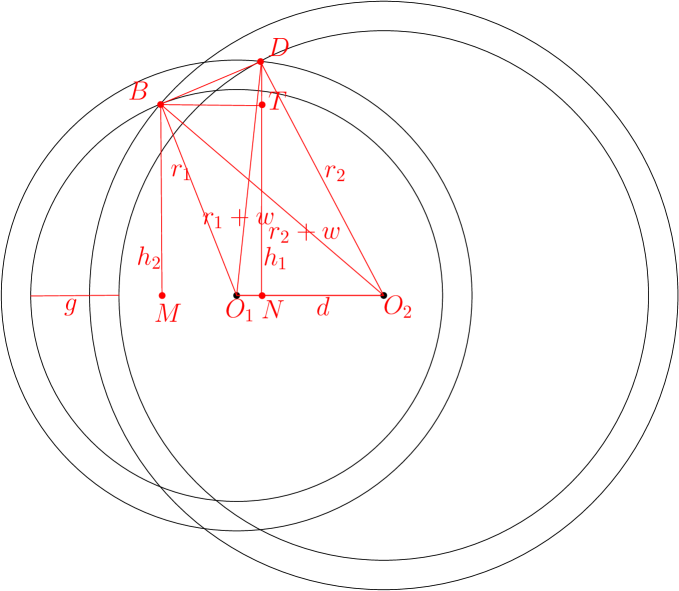
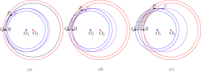
The proof sketch.ย ย ย  For the complete proof see Appendixย A. When wโ‰คdโ‰คr2โˆ’r1+2โ€‹w๐‘ค๐‘‘subscript๐‘Ÿ2subscript๐‘Ÿ12๐‘คw\leq d\leq r_{2}-r_{1}+2w, the intersection region consists of two triangle-like regions. We only bound the triangle-like region โ–ณ~โ€‹Pโ€‹Qโ€‹R~โ–ณ๐‘ƒ๐‘„๐‘…\tilde{\triangle}PQR in the upper half annuli as shown in Figureย 1. We can show that its area is asymptotically upper bounded by the product of its base length |Qโ€‹R|=Oโ€‹(w)๐‘„๐‘…๐‘‚๐‘ค|QR|=O(w) and its height hโ„Žh. We bound hโ„Žh by observing that hโ€‹d2โ„Ž๐‘‘2\frac{hd}{2} is the area of triangle โ–ณโ€‹Pโ€‹O1โ€‹O2โ–ณ๐‘ƒsubscript๐‘‚1subscript๐‘‚2\triangle PO_{1}O_{2} but we can also obtain its area of using Heronโ€™s formula, given its three side lengths. This gives h=Oโ€‹(nโ€‹w/d)โ„Ž๐‘‚๐‘›๐‘ค๐‘‘h=O(n\sqrt{w/d}). Since in this case gโ‰ค2โ€‹w๐‘”2๐‘คg\leq 2w, the intersection area is upper bounded by Oโ€‹(wโ€‹nโ€‹w2(g+w)โ€‹d)๐‘‚๐‘ค๐‘›superscript๐‘ค2๐‘”๐‘ค๐‘‘O\left(wn\sqrt{\frac{w^{2}}{(g+w)d}}\right) as claimed.

Refer to caption
Figure 1. Intersections When d๐‘‘d is Small

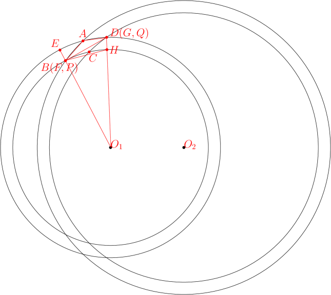
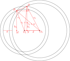
When r2โˆ’r1+2โ€‹wโ‰คdโ‰คr2subscript๐‘Ÿ2subscript๐‘Ÿ12๐‘ค๐‘‘subscript๐‘Ÿ2r_{2}-r_{1}+2w\leq d\leq r_{2}, the intersection region consists of two quadrilateral-like regions. Again we only consider โ–ก~โ€‹Aโ€‹Bโ€‹Cโ€‹D~โ–ก๐ด๐ต๐ถ๐ท\tilde{\square}ABCD in the upper half of the annuli, which is contained in a partial annulus, โ„›~Eโ€‹Fโ€‹Hโ€‹Dsubscript~โ„›๐ธ๐น๐ป๐ท\tilde{\mathscr{R}}_{EFHD}, as shown in Figureย 2.

Refer to caption
(a) Cover an Intersection by A Partial Annulus
Refer to caption
(b) Bound the Length of |Bโ€‹D|๐ต๐ท|BD|
Figure 2. Cover a Quadrilateral-like Region by a Partial Annulus

We show the area of โ„›~Eโ€‹Fโ€‹Hโ€‹Dsubscript~โ„›๐ธ๐น๐ป๐ท\tilde{\mathscr{R}}_{EFHD} is asymptotically bounded by |Bโ€‹H|โ‹…wโ‹…๐ต๐ป๐‘ค|BH|\cdot w, where |Bโ€‹H|๐ต๐ป|BH| is the distance between the two endpoints of the inner arc. We upper bound |Bโ€‹H|๐ต๐ป|BH| by |Bโ€‹D|๐ต๐ท|BD|. We use the algebraic representation of the two annuli, to bound the length of the projection of Bโ€‹D๐ต๐ทBD on the X๐‘‹X-axis by ฮ˜โ€‹(wโ€‹nd)ฮ˜๐‘ค๐‘›๐‘‘\Theta\left(\frac{wn}{d}\right); See Figureย 2. We use Heronโ€™s formula to bound the length of the projection of Bโ€‹D๐ต๐ทBD on the Y๐‘ŒY-axis by Oโ€‹(nโ€‹w2/dโ€‹g)๐‘‚๐‘›superscript๐‘ค2๐‘‘๐‘”O\left(n\sqrt{w^{2}/dg}\right). The maximum of the length of the two projections yields the claimed bound. โˆŽ

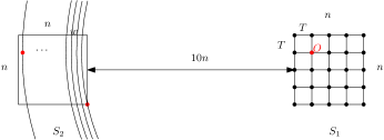
We use Chazelleโ€™s framework to obtain a lower bound for 2D annulus reporting. Let S1subscript๐‘†1S_{1} and S2subscript๐‘†2S_{2} be two squares of side length n๐‘›n that are placed 10โ€‹n10๐‘›10n distance apart and S2subscript๐‘†2S_{2} is directly to the left of S1subscript๐‘†1S_{1}. We generate the annuli as follows. We divide S1subscript๐‘†1S_{1} into a nTร—nT๐‘›๐‘‡๐‘›๐‘‡\frac{n}{T}\times\frac{n}{T} grid where each cell is a square of side length T๐‘‡T. For each grid point, we construct a series of circles as follows. Let O๐‘‚O be a grid point. The first circle generated for O๐‘‚O must pass through a corner of S2subscript๐‘†2S_{2} and not intersect the right side of S2subscript๐‘†2S_{2}, as shown in Figureย 3. Then we create a series of circles centered at O๐‘‚O by increasing the radius by increments of w๐‘คw, for some w<T๐‘ค๐‘‡w<T, as long as it does not intersect the left side of S2subscript๐‘†2S_{2}. Every consecutive two circles defines an annulus centered on O๐‘‚O. We repeat this for every grid cell in S1subscript๐‘†1S_{1} and this makes up our set of queries. The input points are placed uniformly randomly inside S2subscript๐‘†2S_{2}.

Refer to caption
Figure 3. Generate a Family of Annuli at Point O๐‘‚O

We now show that for the annuli we constructed, the intersection of โ„“โ„“\ell annuli is not too large, for some โ„“โ„“\ell we specify later. More precisely we prove the following.

Lemma 4.0.

There exists a large enough constant c๐‘c such that in any subset of โ„“=cโ€‹w2/Tโ„“๐‘superscript๐‘ค2๐‘‡\ell=cw^{2}/\sqrt{T} annuli, we can find two annuli such that their intersection has area Oโ€‹(nโ€‹wโ€‹1T)๐‘‚๐‘›๐‘ค1๐‘‡O\left(nw\sqrt{\frac{1}{T}}\right).

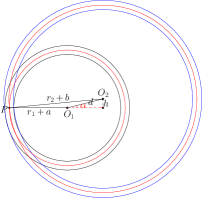
The proof sketch.ย ย ย  For the complete proof see Appendixย B. Let ๐’ฎ๐’ฎ\mathcal{S} be a set of โ„“=cโ€‹w2/Tโ„“๐‘superscript๐‘ค2๐‘‡\ell=cw^{2}/\sqrt{T} annuli. Suppose for the sake of contradiction that we cannot find two annuli in ๐’ฎ๐’ฎ\mathcal{S} whose intersection area is Oโ€‹(nโ€‹wโ€‹1T)๐‘‚๐‘›๐‘ค1๐‘‡O\left(nw\sqrt{\frac{1}{T}}\right). Since by Lemmaย 4.1, the intersection area of any two annuli in our construction with distance ฮฉโ€‹(wโ€‹T)ฮฉ๐‘ค๐‘‡\Omega(wT) is Oโ€‹(nโ€‹wโ€‹1T)๐‘‚๐‘›๐‘ค1๐‘‡O\left(nw\sqrt{\frac{1}{T}}\right). The maximum distance between any two annuli in ๐’ฎ๐’ฎ\mathcal{S} must be oโ€‹(wโ€‹T)๐‘œ๐‘ค๐‘‡o(wT).

Refer to caption
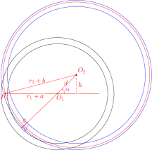
Figure 4. Intersection of Two Annuli

Let P๐‘ƒP be a point in the intersection of annuli in ๐’ฎ๐’ฎ\mathcal{S}. Consider an arbitrary annulus โ„›1โˆˆ๐’ฎsubscriptโ„›1๐’ฎ\mathscr{R}_{1}\in\mathcal{S} centered at O1subscript๐‘‚1O_{1} and another annulus โ„›2โˆˆ๐’ฎsubscriptโ„›2๐’ฎ\mathscr{R}_{2}\in\mathcal{S} centered at O2subscript๐‘‚2O_{2} for some O2โˆ‰Pโ€‹O1subscript๐‘‚2๐‘ƒsubscript๐‘‚1O_{2}\notin PO_{1}. For โ„›1,โ„›2subscriptโ„›1subscriptโ„›2\mathscr{R}_{1},\mathscr{R}_{2} to contain P๐‘ƒP, we must have |Pโ€‹O1|=r1+a,|Pโ€‹O2|=r2+bformulae-sequence๐‘ƒsubscript๐‘‚1subscript๐‘Ÿ1๐‘Ž๐‘ƒsubscript๐‘‚2subscript๐‘Ÿ2๐‘|PO_{1}|=r_{1}+a,|PO_{2}|=r_{2}+b for 0โ‰คa,bโ‰คwformulae-sequence0๐‘Ž๐‘๐‘ค0\leq a,b\leq w. See Figureย 4 for an example. Also |O1โ€‹O2|=dsubscript๐‘‚1subscript๐‘‚2๐‘‘|O_{1}O_{2}|=d, by exploiting the shape of โ–ณโ€‹Pโ€‹O1โ€‹O2โ–ณ๐‘ƒsubscript๐‘‚1subscript๐‘‚2\triangle PO_{1}O_{2} and applying Lemmaย 4.1, we can compute an upper bound for the distance between O2subscript๐‘‚2O_{2} and Pโ€‹O1๐‘ƒsubscript๐‘‚1PO_{1}, namely, h=dโ€‹sinโกฮฑ=oโ€‹(wโ€‹T)โ„Ž๐‘‘๐›ผ๐‘œ๐‘ค๐‘‡h=d\sin\alpha=o(w\sqrt{T}), where ฮฑ๐›ผ\alpha is the angle between O1โ€‹O2subscript๐‘‚1subscript๐‘‚2O_{1}O_{2} and Pโ€‹O1๐‘ƒsubscript๐‘‚1PO_{1}. This implies that ๐’ฎ๐’ฎ\mathcal{S} must fit in a rectangle of size oโ€‹(wโ€‹T)ร—oโ€‹(wโ€‹T)๐‘œ๐‘ค๐‘‡๐‘œ๐‘ค๐‘‡o(wT)\times o(w\sqrt{T}). Since the gird cell size is Tร—T๐‘‡๐‘‡T\times T, only oโ€‹(w2/T)๐‘œsuperscript๐‘ค2๐‘‡o(w^{2}/\sqrt{T}) annuli are contained in such a rectangle, a contradiction. โˆŽ

We are now ready to plug in some parameters in our construction. We set T=w2โ€‹22โ€‹logโกn๐‘‡superscript๐‘ค2superscript22๐‘›T=w^{2}2^{2\sqrt{\log n}}. First, we claim that from each grid cell O๐‘‚O, we can draw ฮ˜โ€‹(n/w)ฮ˜๐‘›๐‘ค\Theta(n/w) circles; Let C1,C2,C3subscript๐ถ1subscript๐ถ2subscript๐ถ3C_{1},C_{2},C_{3}, and C4subscript๐ถ4C_{4} be the corners of S2subscript๐‘†2S_{2} sorted increasingly according to their distance to O๐‘‚O. As S1subscript๐‘†1S_{1} and S2subscript๐‘†2S_{2} are placed 10โ€‹n10๐‘›10n distance apart, an elementary geometric calculation reveals that C1subscript๐ถ1C_{1} and C2subscript๐ถ2C_{2} are vertices of the right edge of S2subscript๐‘†2S_{2}, meaning, the smallest circle that we draw from O๐‘‚O passes through C2subscript๐ถ2C_{2} and we keep drawing circles, by incrementing their radii by w๐‘คw until we are about to draw a circle that is about to contain C3subscript๐ถ3C_{3}. We can see that |Oโ€‹C3|โˆ’|Oโ€‹C2|=ฮ˜โ€‹(n)๐‘‚subscript๐ถ3๐‘‚subscript๐ถ2ฮ˜๐‘›|OC_{3}|-|OC_{2}|=\Theta(n) and thus we draw ฮ˜โ€‹(n/w)ฮ˜๐‘›๐‘ค\Theta(n/w) circles from O๐‘‚O. As we have ฮ˜โ€‹((n/T)2)ฮ˜superscript๐‘›๐‘‡2\Theta((n/T)^{2}) grid cells, it thus follows that we have ฮ˜โ€‹(n3/(T2โ€‹w))ฮ˜superscript๐‘›3superscript๐‘‡2๐‘ค\Theta(n^{3}/(T^{2}w)) annuli in our construction.

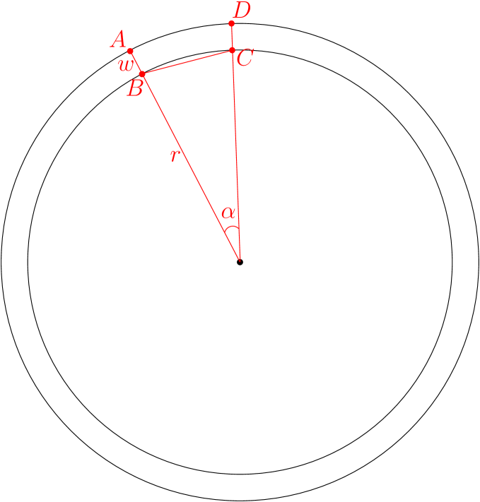
Also by our construction, the area of each annulus within S2subscript๐‘†2S_{2} is ฮ˜โ€‹(wโ€‹n)ฮ˜๐‘ค๐‘›\Theta(wn). To see this, let P๐‘ƒP be an arbitrary point in S1subscript๐‘†1S_{1}, let A,B๐ด๐ตA,B be the intersections of some circle centered at P๐‘ƒP as in Figureย 5.

Refer to caption
Figure 5. The Angle of an Annulus

We connect Aโ€‹B๐ด๐ตAB and let C๐ถC be the center of Aโ€‹B๐ด๐ตAB. Let ฮฑ=โˆ โ€‹Aโ€‹Pโ€‹C๐›ผโˆ ๐ด๐‘ƒ๐ถ\alpha=\angle{APC}. In the triangle โ–ณโ€‹Aโ€‹Bโ€‹Pโ–ณ๐ด๐ต๐‘ƒ\triangle ABP, all the sides are within constant factors of each other and thus ฮฑ=ฮ˜โ€‹(1)๐›ผฮ˜1\alpha=\Theta(1) and so the area of the annulus inside S2subscript๐‘†2S_{2} is at least a constant fraction of the area of the entire annulus.

Suppose we have a data structure that answers 2D annulus reporting queries in Qโ€‹(n)+Oโ€‹(k)๐‘„๐‘›๐‘‚๐‘˜Q(n)+O(k) time. We set w=cโ€ฒโ€‹Qโ€‹(n)๐‘คsuperscript๐‘โ€ฒ๐‘„๐‘›w=c^{\prime}Q(n) for a large enough constant cโ€ฒsuperscript๐‘โ€ฒc^{\prime} such that the area of each annulus within S2subscript๐‘†2S_{2} is at least ฮ˜โ€‹(wโ€‹n)>8โ€‹nโ€‹Qโ€‹(n)ฮ˜๐‘ค๐‘›8๐‘›๐‘„๐‘›\Theta(wn)>8nQ(n). By Lemmaย 2.4, if we sample n๐‘›n points uniformly at random in S2subscript๐‘†2S_{2}, then with probability more than 1/2121/2, each annulus contains at least Qโ€‹(n)๐‘„๐‘›Q(n) points.

Also by our construction, the total number of intersections of two annuli is bounded by Oโ€‹(n6)๐‘‚superscript๐‘›6O(n^{6}) and by our choice of T๐‘‡T, Oโ€‹(nโ€‹wโ€‹1T)=Oโ€‹(n2logโกn)๐‘‚๐‘›๐‘ค1๐‘‡๐‘‚๐‘›superscript2๐‘›O\left(nw\sqrt{\frac{1}{T}}\right)=O\left(\frac{n}{2^{\sqrt{\log n}}}\right). Then by Lemmaย 2.3 and Lemmaย 4.2, with probability >12absent12>\frac{1}{2}, a point set of size n๐‘›n picked uniformly at random in S2subscript๐‘†2S_{2} satisfies that the number of points in any of the intersection of cโ€‹w2/T๐‘superscript๐‘ค2๐‘‡cw^{2}/\sqrt{T} annuli is no more than 9โ€‹logโกn9๐‘›9\sqrt{\log n}.

Now by union bound, there exist ฮ˜โ€‹(n3wโ€‹T2)ฮ˜superscript๐‘›3๐‘คsuperscript๐‘‡2\Theta\left(\frac{n^{3}}{wT^{2}}\right) point sets such that each set is the output of some 2D annulus query and each set contains at least Qโ€‹(n)๐‘„๐‘›Q(n) points. Furthermore, the intersection of any cโ€‹w2/T๐‘superscript๐‘ค2๐‘‡cw^{2}/\sqrt{T} sets is bounded by 9โ€‹logโกn9๐‘›9\sqrt{\log n}. Then by Theoremย 2.1, we obtain a lower bound of

Sโ€‹(n)=ฮฉโ€‹(Qโ€‹(n)โ€‹n3โ€‹Twโ€‹T2โ€‹w2โ€‹2Oโ€‹(logโกn))=ฮฉ๐‘œโ€‹(n3Qโ€‹(n)5).๐‘†๐‘›ฮฉ๐‘„๐‘›superscript๐‘›3๐‘‡๐‘คsuperscript๐‘‡2superscript๐‘ค2superscript2๐‘‚๐‘›๐‘œฮฉsuperscript๐‘›3๐‘„superscript๐‘›5S(n)=\Omega\left(\frac{Q(n)n^{3}\sqrt{T}}{wT^{2}w^{2}2^{O\left(\sqrt{\log n}\right)}}\right)=\overset{\scriptscriptstyle o}{\Omega}\left(\frac{n^{3}}{Q(n)^{5}}\right).

This proves the following theorem about 2D annulus reporting.

Theorem 4.3.

Any data structure that solves 2D annulus reporting on point set of size n๐‘›n with query time Qโ€‹(n)+Oโ€‹(k)๐‘„๐‘›๐‘‚๐‘˜Q(n)+O(k), where k๐‘˜k is the output size, must use ฮฉ๐‘œโ€‹(n3/Qโ€‹(n)5)๐‘œฮฉsuperscript๐‘›3๐‘„superscript๐‘›5\overset{\scriptscriptstyle o}{\Omega}\left({n^{3}}/{Q(n)^{5}}\right) space.

So for any data structure that solves 2D annulus reporting in time Qโ€‹(n)=logOโ€‹(1)โกn๐‘„๐‘›superscript๐‘‚1๐‘›Q(n)=\log^{O(1)}n, Theoremย 4.3 implies that ฮฉ๐‘œโ€‹(n3)๐‘œฮฉsuperscript๐‘›3\overset{\scriptscriptstyle o}{\Omega}\left(n^{3}\right) space must be used.

4.2. 2D Annulus Stabbing

Modifications similar to those done in Subsectionย 3.2 can be used to obtain the following lower bound.

Theorem 4.4.

Any data structure that solves the 2D annulus stabbing problem with query time Qโ€‹(n)+Oโ€‹(k)๐‘„๐‘›๐‘‚๐‘˜Q(n)+O(k), where k๐‘˜k is the output size, must use Sโ€‹(n)=ฮฉโ€‹(n3/2/Qโ€‹(n)3/4)๐‘†๐‘›ฮฉsuperscript๐‘›32๐‘„superscript๐‘›34S(n)=\Omega(n^{3/2}/Q(n)^{3/4}) space.

Proof.

We use Afshaniโ€™s lower bound framework as in Theoremย 2.2. We construct annuli similar to the way as we did in the proof of Theoremย 4.3, but with some differences. Let S1subscript๐‘†1S_{1} be a unit square, we decompose S1subscript๐‘†1S_{1} into a grid where each grid cell is a square of size Tร—T๐‘‡๐‘‡T\times T, for some parameter T๐‘‡T to be determined later. Let S2subscript๐‘†2S_{2} be another unit square to the left of S1subscript๐‘†1S_{1} with distance 101010. For each grid point in S1subscript๐‘†1S_{1}, we generate a family of circles where the first circle is the first one tangent to the right side of S2subscript๐‘†2S_{2}. See Figureย 6 for an example.

Refer to caption
Figure 6. Generate a Family of Annuli at Point O๐‘‚O

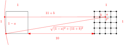
Let r0subscript๐‘Ÿ0r_{0} be the radius of this circle. We generate other circles by increasing the radius by w๐‘คw each time. The last circle is the one with radius at least r0+(122โˆ’9)subscript๐‘Ÿ01229r_{0}+(\sqrt{122}-9). The choice of constant 122โˆ’91229\sqrt{122}-9 is due to the following. Consider a point P๐‘ƒP in the upper half of S1subscript๐‘†1S_{1}, let a๐‘Ža (resp. b๐‘b) be the distance from P๐‘ƒP to the upper (resp. left) side of S1subscript๐‘†1S_{1}. The case for the lower half of S1subscript๐‘†1S_{1} is symmetric. Consider the last circle intersecting S2subscript๐‘†2S_{2} only at the corners. See Figureย 7 for an example.

Refer to caption
Figure 7. The Last Valid Circle

The difference of radius lengths between the last circle and the first circle is

f=(1โˆ’a)2+(11+b)2โˆ’10โˆ’b.๐‘“superscript1๐‘Ž2superscript11๐‘210๐‘f=\sqrt{(1-a)^{2}+(11+b)^{2}}-10-b.

Simple analysis shows that fโ‰ค122โˆ’10๐‘“12210f\leq\sqrt{122}-10. This shows as long as the last circle has radius at least 122โˆ’9+r01229subscript๐‘Ÿ0\sqrt{122}-9+r_{0}, it is completely outside of S2subscript๐‘†2S_{2}. Like we did previously, we consider the region between two consecutive annuli to be an annulus. Note that by our construction, for any point in S2subscript๐‘†2S_{2}, it is contained in one of the annuli we generated for a given grid point. The total number of annuli we have generated is therefore

(1T+1)2โ‹…122โˆ’9w.โ‹…superscript1๐‘‡121229๐‘ค\left(\frac{1}{T}+1\right)^{2}\cdot\frac{\sqrt{122}-9}{w}.

We set T=1/(2โ€‹Qโ€‹(n)โˆ’1)๐‘‡12๐‘„๐‘›1T=1/(2\sqrt{Q(n)}-1) and w=4โ€‹(122โˆ’9)โ€‹Qโ€‹(n)/n๐‘ค41229๐‘„๐‘›๐‘›w=4(\sqrt{122}-9)Q(n)/n. Then the total number of annuli we have generated is n๐‘›n. Furthermore, each query point is contained in t=(1/T+1)2โ‰ฅQโ€‹(n)๐‘กsuperscript1๐‘‡12๐‘„๐‘›t=(1/T+1)^{2}\geq Q(n) annuli.

To use Lemmaย 4.1, we require wโ‰คT๐‘ค๐‘‡w\leq T, which implies Qโ€‹(n)=Oโ€‹(n2/3)๐‘„๐‘›๐‘‚superscript๐‘›23Q(n)=O(n^{2/3}), the intersection area of two annuli in our construction is upper bounded by v=Oโ€‹(wโ€‹wT)=Oโ€‹(Qโ€‹(n)7/4/n3/2)๐‘ฃ๐‘‚๐‘ค๐‘ค๐‘‡๐‘‚๐‘„superscript๐‘›74superscript๐‘›32v=O(w\sqrt{\frac{w}{T}})=O(Q(n)^{7/4}/n^{3/2}). Then by Theoremย 2.2,

Sโ€‹(n)=ฮฉโ€‹(tv)=ฮฉโ€‹(n3/2Qโ€‹(n)3/4).โˆŽ๐‘†๐‘›ฮฉ๐‘ก๐‘ฃฮฉsuperscript๐‘›32๐‘„superscript๐‘›34S(n)=\Omega\left(\frac{t}{v}\right)=\Omega\left(\frac{n^{3/2}}{Q(n)^{3/4}}\right).\qed

So for any data structure that solves the 2D annulus stabbing problem using Oโ€‹(n)๐‘‚๐‘›O(n) space, Theoremย 4.4 implies that its query time must be Qโ€‹(n)=ฮฉโ€‹(n2/3)๐‘„๐‘›ฮฉsuperscript๐‘›23Q(n)=\Omega(n^{2/3}).

5. Conclusion and Open Problems

We investigated lower bounds for range searching with polynomial slabs and annuli in โ„2superscriptโ„2\mathbb{R}^{2}. We showed space-time tradeoff bounds of Sโ€‹(n)=ฮฉ๐‘œโ€‹(nฮ”+1/Qโ€‹(n)(ฮ”+3)โ€‹ฮ”/2)๐‘†๐‘›๐‘œฮฉsuperscript๐‘›ฮ”1๐‘„superscript๐‘›ฮ”3ฮ”2S(n)=\overset{\scriptscriptstyle o}{\Omega}(n^{\Delta+1}/Q(n)^{(\Delta+3)\Delta/2}) and Sโ€‹(n)=ฮฉ๐‘œโ€‹(n3/Qโ€‹(n)5)๐‘†๐‘›๐‘œฮฉsuperscript๐‘›3๐‘„superscript๐‘›5S(n)=\overset{\scriptscriptstyle o}{\Omega}(n^{3}/Q(n)^{5}) for them respectively. Both of these bounds are almost tight in the โ€œfast queryโ€ case, i.e., when Qโ€‹(n)=logOโ€‹(1)โกn๐‘„๐‘›superscript๐‘‚1๐‘›Q(n)=\log^{O(1)}n (up to a noโ€‹(1)superscript๐‘›๐‘œ1n^{o(1)} factor). This refutes the conjecture of the existence of data structure that can solve semialgebraic range searching in โ„dsuperscriptโ„๐‘‘\mathbb{R}^{d} using O๐‘œโ€‹(nd)๐‘œ๐‘‚superscript๐‘›๐‘‘\overset{\scriptscriptstyle o}{O}(n^{d}) space and logOโ€‹(1)โกnsuperscript๐‘‚1๐‘›\log^{O(1)}n query time. We also studied the โ€œdualโ€ polynomial slab stabbing and annulus stabbing problems. For these two problems, we obtained lower bounds Sโ€‹(n)=ฮฉโ€‹(n1+2/(ฮ”+1)/Qโ€‹(n)2/ฮ”)๐‘†๐‘›ฮฉsuperscript๐‘›12ฮ”1๐‘„superscript๐‘›2ฮ”S(n)=\Omega(n^{1+2/(\Delta+1)}/Q(n)^{2/\Delta}) and Sโ€‹(n)=ฮฉโ€‹(n3/2/Qโ€‹(n)3/4)๐‘†๐‘›ฮฉsuperscript๐‘›32๐‘„superscript๐‘›34S(n)=\Omega(n^{3/2}/Q(n)^{3/4}) respectively. These bounds are tight when Sโ€‹(n)=Oโ€‹(n)๐‘†๐‘›๐‘‚๐‘›S(n)=O(n). Our work, however, brings out some very interesting open problems.

To get the lower bounds for the polynomial slabs, we only considered univariate polynomials of degree ฮ”ฮ”\Delta. In this setting, the number of coefficients is at most ฮ”+1ฮ”1\Delta+1, and we have also assumed they are all independent. It would be interesting to see if similar lower bounds can be obtained under more general settings. In particular, as the maximum number of coefficients of a bivaraite polynomial of degree ฮ”ฮ”\Delta is (ฮ”+22)binomialฮ”22\binom{\Delta+2}{2}, it would interesting to see if a ฮฉ๐‘œโ€‹(n(ฮ”+22)โˆ’1)๐‘œฮฉsuperscript๐‘›binomialฮ”221\overset{\scriptscriptstyle o}{\Omega}(n^{\binom{\Delta+2}{2}-1}) space lower bound can be obtained for the โ€œfast queryโ€ case.

It would also be interesting to consider space-time trade-offs. For instance, by combining the known โ€œfast queryโ€ and โ€œlow spaceโ€ solutions for 2D annulus reporting, one can obtain data structures with trade-off curve Sโ€‹(n)=O~โ€‹(n3/Qโ€‹(n)4)๐‘†๐‘›~๐‘‚superscript๐‘›3๐‘„superscript๐‘›4S(n)=\tilde{O}(n^{3}/Q(n)^{4}), however, our lower bound is Sโ€‹(n)=ฮฉ๐‘œโ€‹(n3/Qโ€‹(n)5)๐‘†๐‘›๐‘œฮฉsuperscript๐‘›3๐‘„superscript๐‘›5S(n)=\overset{\scriptscriptstyle o}{\Omega}(n^{3}/Q(n)^{5}) and it is not clear which of these bounds is closer to truth. For the annulus searching problem in โ„2superscriptโ„2\mathbb{R}^{2}, in our lower bound proof, we considered a random input point set, since in most cases a random point set is the hardest input instance and our analysis seems to be tight, we therefore conjecture that our lower bound could be tight, at least when Qโ€‹(n)๐‘„๐‘›Q(n) is small enough. We believe that it should be possible to obtain the trade-off curve of Sโ€‹(n)=O~โ€‹(n3/Qโ€‹(n)5)๐‘†๐‘›~๐‘‚superscript๐‘›3๐‘„superscript๐‘›5S(n)=\tilde{O}(n^{3}/Q(n)^{5}) when the input points are uniformly random in the unit square and Qโ€‹(n)๐‘„๐‘›Q(n) is not too big.

Finally, another interesting direction is to study the lower bound for the counting variant of semialgebraic range searching.

Acknowledgements.
The authors would like to thank Esther Ezra for sparking the initial ideas behind the proof.

References

  • (1)
  • Afshani (2012) Peyman Afshani. 2012. Improved Pointer Machine and I/O Lower Bounds for Simplex Range Reporting and Related Problems. In Proceedings of the Twenty-Eighth Annual Symposium on Computational Geometry (Chapel Hill, North Carolina, USA) (SoCG โ€™12). Association for Computing Machinery, New York, NY, USA, 339โ€“346. https://doi.org/10.1145/2261250.2261301
  • Afshani and Driemel (2018) Peyman Afshani and Anne Driemel. 2018. On the complexity of range searching among curves. In Proceedings of the Twenty-Ninth Annual ACM-SIAM Symposium on Discrete Algorithms. SIAM, Philadelphia, PA, 898โ€“917. https://doi.org/10.1137/1.9781611975031.58
  • Agarwal (2017) Pankajย K. Agarwal. 2017. Simplex Range Searching and Its Variants: A Review. Springer International Publishing, Cham, 1โ€“30. https://doi.org/10.1007/978-3-319-44479-6_1
  • Agarwal etย al. (2019) Pankajย K. Agarwal, Boris Aronov, Esther Ezra, and Joshua Zahl. 2019. An efficient algorithm for generalized polynomial partitioning and its applications. In 35th International Symposium on Computational Geometry. LIPIcs. Leibniz Int. Proc. Inform., Vol.ย 129. Schloss Dagstuhl. Leibniz-Zent. Inform., Wadern, Art. No. 5, 14.
  • Agarwal and Matouลกek (1994) Pankajย K. Agarwal and Jiล™รญ Matouลกek. 1994. On range searching with semialgebraic sets. Discrete Comput. Geom. 11, 4 (1994), 393โ€“418. https://doi.org/10.1007/BF02574015
  • Agarwal etย al. (2013) Pankajย K. Agarwal, Jiล™รญ Matouลกek, and Micha Sharir. 2013. On range searching with semialgebraic sets. II. SIAM J. Comput. 42, 6 (2013), 2039โ€“2062. https://doi.org/10.1137/120890855
  • Chan (2012) Timothyย M. Chan. 2012. Optimal partition trees. Discrete Comput. Geom. 47, 4 (2012), 661โ€“690. https://doi.org/10.1007/s00454-012-9410-z
  • Chazelle (1989) Bernard Chazelle. 1989. Lower bounds on the complexity of polytope range searching. J. Amer. Math. Soc. 2, 4 (1989), 637โ€“666. https://doi.org/10.2307/1990891
  • Chazelle (1990) Bernard Chazelle. 1990. Lower bounds for orthogonal range searching. I. The reporting case. J. Assoc. Comput. Mach. 37, 2 (1990), 200โ€“212. https://doi.org/10.1145/77600.77614
  • Chazelle (1993) Bernard Chazelle. 1993. Cutting Hyperplanes for Divide-and-Conquer. Discrete Comput. Geom. 9, 2 (Dec. 1993), 145โ€“158. https://doi.org/10.1007/BF02189314
  • Chazelle (2018) Bernard Chazelle. 2018. Cuttings. In Handbook of Data Structures and Applications, Dineshย P. Mehta and Sartaj Sahni (Eds.). Chapman and Hall/CRC. https://doi.org/10.1201/9781315119335 Second edition.
  • Chazelle and Friedman (1990) B. Chazelle and J. Friedman. 1990. A deterministic view of random sampling and its use in geometry. Combinatorica 10, 3 (1990), 229โ€“249. https://doi.org/10.1007/BF02122778
  • Chazelle and Rosenberg (1996) Bernard Chazelle and Burton Rosenberg. 1996. Simplex range reporting on a pointer machine. Comput. Geom. 5, 5 (1996), 237โ€“247. https://doi.org/10.1016/0925-7721(95)00002-X
  • Chazelle and Welzl (1989) Bernard Chazelle and Emo Welzl. 1989. Quasi-optimal range searching in spaces of finite VC-dimension. Discrete Comput. Geom. 4, 5 (1989), 467โ€“489. https://doi.org/10.1007/BF02187743
  • Clarkson (1987) Kennethย L. Clarkson. 1987. New applications of random sampling in computational geometry. Discrete Comput. Geom. 2, 2 (1987), 195โ€“222. https://doi.org/10.1007/BF02187879
  • Dvir (2009) Zeev Dvir. 2009. On the size of Kakeya sets in finite fields. J. Amer. Math. Soc. 22, 4 (2009), 1093โ€“1097. https://doi.org/10.1090/S0894-0347-08-00607-3
  • Goodman etย al. (2018) Jacobย E. Goodman, Joseph Oโ€™Rourke, and Csabaย D. Tรณth (Eds.). 2018. Handbook of discrete and computational geometry. CRC Press, Boca Raton, FL. xxi+1927 pages. https://doi.org/10.1201/9781315119601 Third edition.
  • Guth (2015) Larry Guth. 2015. Polynomial partitioning for a set of varieties. Math. Proc. Cambridge Philos. Soc. 159, 3 (2015), 459โ€“469. https://doi.org/10.1017/S0305004115000468
  • Guth and Katz (2015) Larry Guth and Netsย Hawk Katz. 2015. On the Erdล‘s distinct distances problem in the plane. Ann. of Math. (2) 181, 1 (2015), 155โ€“190. https://doi.org/10.4007/annals.2015.181.1.2
  • Haussler and Welzl (1986) D Haussler and E Welzl. 1986. Epsilon-Nets and Simplex Range Queries. In Proceedings of the Second Annual Symposium on Computational Geometry (Yorktown Heights, New York, USA) (SCG โ€™86). Association for Computing Machinery, New York, NY, USA, 61โ€“71. https://doi.org/10.1145/10515.10522
  • Matouลกek (1991) Jiล™รญ Matouลกek. 1991. Cutting hyperplane arrangements. Discrete Comput. Geom. 6, 5 (1991), 385โ€“406. https://doi.org/10.1007/BF02574697
  • Matouลกek (1993) Jiล™รญ Matouลกek. 1993. Range searching with efficient hierarchical cuttings. Discrete Comput. Geom. 10, 2 (1993), 157โ€“182. https://doi.org/10.1007/BF02573972
  • Matouลกek and Patรกkovรก (2015) Jiล™รญ Matouลกek and Zuzana Patรกkovรก. 2015. Multilevel polynomial partitions and simplified range searching. Discrete Comput. Geom. 54, 1 (2015), 22โ€“41. https://doi.org/10.1007/s00454-015-9701-2
  • Welzl (1988) Emo Welzl. 1988. Partition trees for triangle counting and other range searching problems. In Proceedings of the Fourth Annual Symposium on Computational Geometry (Urbana, IL, 1988). ACM, New York, 23โ€“33. https://doi.org/10.1145/73393.73397
  • Willard (1982) Danย E. Willard. 1982. Polygon retrieval. SIAM J. Comput. 11, 1 (1982), 149โ€“165. https://doi.org/10.1137/0211012
  • Yao and Yao (1985) Aย C Yao and Fย F Yao. 1985. A General Approach to D-Dimensional Geometric Queries. In Proceedings of the Seventeenth Annual ACM Symposium on Theory of Computing (Providence, Rhode Island, USA) (STOC โ€™85). Association for Computing Machinery, New York, NY, USA, 163โ€“168. https://doi.org/10.1145/22145.22163

Appendix A Proof of Lemmaย 4.1

See 4.1

Proof.

First note that for two annuli to intersect, dโ‰ฅr2โˆ’r1โˆ’w๐‘‘subscript๐‘Ÿ2subscript๐‘Ÿ1๐‘คd\geq r_{2}-r_{1}-w. When wโ‰คdโ‰คr2โˆ’r1+2โ€‹w๐‘ค๐‘‘subscript๐‘Ÿ2subscript๐‘Ÿ12๐‘คw\leq d\leq r_{2}-r_{1}+2w, observe that gโ‰ค2โ€‹w๐‘”2๐‘คg\leq 2w and the intersections are all bounded by a two triangle-like regions. We consider the triangle like region โ–ณ~โ€‹Pโ€‹Qโ€‹R~โ–ณ๐‘ƒ๐‘„๐‘…\tilde{\triangle}PQR in the upper half of the annuli as shown in Figureย 8. The area of the other triangle like region can be bounded symmetrically.
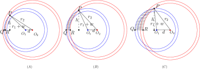
Refer to caption
Figure 8. Intersections When d๐‘‘d is Small

To upper bound its area, we first compute its โ€œheightโ€ hโ„Žh. Consider โ–ณโ€‹Pโ€‹O1โ€‹O2โ–ณ๐‘ƒsubscript๐‘‚1subscript๐‘‚2\triangle PO_{1}O_{2}, by Heronโ€™s Formula, its area is

Aโ–ณโ€‹Pโ€‹O1โ€‹O2subscript๐ดโ–ณ๐‘ƒsubscript๐‘‚1subscript๐‘‚2\displaystyle A_{\triangle PO_{1}O_{2}} =r1+r2+w+d2โ‹…r2+dโˆ’r1โˆ’w2โ‹…r1+d+wโˆ’r22โ‹…r1+r2+wโˆ’d2absentโ‹…subscript๐‘Ÿ1subscript๐‘Ÿ2๐‘ค๐‘‘2subscript๐‘Ÿ2๐‘‘subscript๐‘Ÿ1๐‘ค2subscript๐‘Ÿ1๐‘‘๐‘คsubscript๐‘Ÿ22subscript๐‘Ÿ1subscript๐‘Ÿ2๐‘ค๐‘‘2\displaystyle=\sqrt{\frac{r_{1}+r_{2}+w+d}{2}\cdot\frac{r_{2}+d-r_{1}-w}{2}\cdot\frac{r_{1}+d+w-r_{2}}{2}\cdot\frac{r_{1}+r_{2}+w-d}{2}}
=Oโ€‹(r2โ‹…dโ‹…wโ‹…r1)absent๐‘‚โ‹…subscript๐‘Ÿ2๐‘‘๐‘คsubscript๐‘Ÿ1\displaystyle=O(\sqrt{r_{2}\cdot d\cdot w\cdot r_{1}})
=Oโ€‹(nโ€‹dโ€‹w),absent๐‘‚๐‘›๐‘‘๐‘ค\displaystyle=O\left(n\sqrt{dw}\right),

where the second equality follows from

dโ‰คr2โˆ’r1+2โ€‹w๐‘‘subscript๐‘Ÿ2subscript๐‘Ÿ12๐‘ค\displaystyle d\leq r_{2}-r_{1}+2w~{} โŸนr1+r2+w+dโ‰ค2โ€‹r2+3โ€‹wโ‰ค5โ€‹r2,absentsubscript๐‘Ÿ1subscript๐‘Ÿ2๐‘ค๐‘‘2subscript๐‘Ÿ23๐‘ค5subscript๐‘Ÿ2\displaystyle\implies~{}r_{1}+r_{2}+w+d\leq 2r_{2}+3w\leq 5r_{2},
r2โˆ’r1โˆ’wโ‰คdsubscript๐‘Ÿ2subscript๐‘Ÿ1๐‘ค๐‘‘\displaystyle r_{2}-r_{1}-w\leq d~{} โŸนr2+dโˆ’r1โˆ’wโ‰ค2โ€‹d,absentsubscript๐‘Ÿ2๐‘‘subscript๐‘Ÿ1๐‘ค2๐‘‘\displaystyle\implies~{}r_{2}+d-r_{1}-w\leq 2d,
dโ‰คr2โˆ’r1+2โ€‹w๐‘‘subscript๐‘Ÿ2subscript๐‘Ÿ12๐‘ค\displaystyle d\leq r_{2}-r_{1}+2w~{} โŸนr1+dโˆ’r2+wโ‰ค3โ€‹w,absentsubscript๐‘Ÿ1๐‘‘subscript๐‘Ÿ2๐‘ค3๐‘ค\displaystyle\implies~{}r_{1}+d-r_{2}+w\leq 3w,
r2โˆ’r1โˆ’wโ‰คdsubscript๐‘Ÿ2subscript๐‘Ÿ1๐‘ค๐‘‘\displaystyle r_{2}-r_{1}-w\leq d~{} โŸนr1+r2+wโˆ’dโ‰ค2โ€‹r1+2โ€‹wโ‰ค4โ€‹r1.absentsubscript๐‘Ÿ1subscript๐‘Ÿ2๐‘ค๐‘‘2subscript๐‘Ÿ12๐‘ค4subscript๐‘Ÿ1\displaystyle\implies~{}r_{1}+r_{2}+w-d\leq 2r_{1}+2w\leq 4r_{1}.

Then we bound hโ„Žh by

h=2โ€‹Aโ–ณโ€‹Pโ€‹O1โ€‹O2d=Oโ€‹(nโ€‹wd).โ„Ž2subscript๐ดโ–ณ๐‘ƒsubscript๐‘‚1subscript๐‘‚2๐‘‘๐‘‚๐‘›๐‘ค๐‘‘h=\frac{2A_{\triangle PO_{1}O_{2}}}{d}=O\left(n\sqrt{\frac{w}{d}}\right).

To bound the area of โ–ณ~โ€‹Pโ€‹Qโ€‹R~โ–ณ๐‘ƒ๐‘„๐‘…\tilde{\triangle}PQR, we move the outer circle of the annulus centered at O1subscript๐‘‚1O_{1} along O1โ€‹O2subscript๐‘‚1subscript๐‘‚2O_{1}O_{2} such that it passes R๐‘…R as in Figureย 9. Let S๐‘†S be a point in this new circle such that Pโ€‹SโˆฅQโ€‹Rconditional๐‘ƒ๐‘†๐‘„๐‘…PS\parallel QR. The area of region Pโ€‹Sโ€‹Rโ€‹Q๐‘ƒ๐‘†๐‘…๐‘„PSRQ formed by the outer circle of the annulus centered at O1subscript๐‘‚1O_{1} and the new circle as well as Pโ€‹S๐‘ƒ๐‘†PS and Qโ€‹R๐‘„๐‘…QR, i.e., the shaded region in Figureย 9, is Oโ€‹(wโ€‹h)๐‘‚๐‘คโ„ŽO(wh) by a simple integral argument. Since the curvature of the inner circle of the annulus centered at O2subscript๐‘‚2O_{2} is no larger than that of the outer circle of O1subscript๐‘‚1O_{1} since r2โ‰ฅr1+wsubscript๐‘Ÿ2subscript๐‘Ÿ1๐‘คr_{2}\geq r_{1}+w, โ–ณ~โ€‹Pโ€‹Qโ€‹R~โ–ณ๐‘ƒ๐‘„๐‘…\tilde{\triangle}PQR is contained in this region. So Aโ–ณ~โ€‹Pโ€‹Qโ€‹R=Oโ€‹(wโ€‹h)=Oโ€‹(nโ€‹wโ€‹w/d)=Oโ€‹(nโ€‹wโ€‹w2/(g+w)โ€‹d)subscript๐ด~โ–ณ๐‘ƒ๐‘„๐‘…๐‘‚๐‘คโ„Ž๐‘‚๐‘›๐‘ค๐‘ค๐‘‘๐‘‚๐‘›๐‘คsuperscript๐‘ค2๐‘”๐‘ค๐‘‘A_{\tilde{\triangle}PQR}=O(wh)=O(nw\sqrt{w/d})=O(nw\sqrt{w^{2}/(g+w)d}).

Refer to caption
Figure 9. Bound the Intersection Area for Small d๐‘‘d

In the case r2โˆ’r1+2โ€‹w<d<r2subscript๐‘Ÿ2subscript๐‘Ÿ12๐‘ค๐‘‘subscript๐‘Ÿ2r_{2}-r_{1}+2w<d<r_{2}, the intersections consist of two quadrilateral-like regions, one at the upper half and the other at the lower half. In this case, g>2โ€‹w๐‘”2๐‘คg>2w. We show how to bound the area of the quadrilateral-like region at the upper half, the other one can be bounded symmetrically.

First note that each quadrilateral-like region โ–ก~โ€‹Aโ€‹Bโ€‹Cโ€‹D~โ–ก๐ด๐ต๐ถ๐ท\tilde{\square}{ABCD} is contained in a partial annulus as in Figureย 10. We generate this partial annulus by shooting a ray from the center O1subscript๐‘‚1O_{1} and connect a point P๐‘ƒP in ยฟ Aโ€‹B๐ด๐ต\textstyle AB , such that โ–ก~โ€‹Aโ€‹Bโ€‹Cโ€‹D~โ–ก๐ด๐ต๐ถ๐ท\tilde{\square}ABCD is completely to the right of this ray, to create the left boundary Eโ€‹F๐ธ๐นEF, where E๐ธE is a point in the outer circle of the annulus โ„›1subscriptโ„›1\mathscr{R}_{1} centered at O1subscript๐‘‚1O_{1} and F๐นF is a point in the inner circle of annulus โ„›1subscriptโ„›1\mathscr{R}_{1}. And similarly, shoot another ray and connect a point Q๐‘„Q in ยฟ Cโ€‹D๐ถ๐ท\textstyle CD to create the right boundary Gโ€‹H๐บ๐ปGH. Again, G๐บG is a point in the outer circle of annulus โ„›1subscriptโ„›1\mathscr{R}_{1} and H๐ปH is a point in the inner circle of annulus โ„›1subscriptโ„›1\mathscr{R}_{1}. Note that since d<r2๐‘‘subscript๐‘Ÿ2d<r_{2}, by elementary geometry, P๐‘ƒP can only be B๐ตB and Q๐‘„Q can only be D๐ทD as in Figureย 10.

Refer to caption
(a) Cover an Intersection by A Partial Annulus
Refer to caption
(b) A Partial Annulus Example
Figure 10. Cover a Quadrilateral-like Region by a Partial Annulus

First, we observe that the area of the partial annulus is bounded by the product of the width of the annulus, w๐‘คw, and the length Fโ€‹H๐น๐ปFH, within some constant factor.

To see this, consider the possible partial annulus generated by any two annuli, see Figureย 10 for an example. One important observation is that for any intersection, the angle ฮฑ๐›ผ\alpha of the partial annulus containing it is no more than ฯ€๐œ‹\pi. The area of the partial annulus is clearly ฮฑโ€‹(rโ€‹w+w2/2)=ฮ˜โ€‹(rโ€‹wโ€‹ฮฑ)๐›ผ๐‘Ÿ๐‘คsuperscript๐‘ค22ฮ˜๐‘Ÿ๐‘ค๐›ผ\alpha(rw+w^{2}/2)=\Theta(rw\alpha). Note that for 0โ‰คฮฑโ‰คฯ€0๐›ผ๐œ‹0\leq\alpha\leq\pi, let ฮฒ=ฮฑ/2๐›ฝ๐›ผ2\beta=\alpha/2, it is a simple fact that

12โ€‹ฮฒโ‰คsinโกฮฒโ‰คฮฒ12๐›ฝ๐›ฝ๐›ฝ\frac{1}{2}\beta\leq\sin\beta\leq\beta

for 0โ‰คฮฒโ‰คฯ€/20๐›ฝ๐œ‹20\leq\beta\leq\pi/2. So for ฮฒ๐›ฝ\beta in this range, sinโกฮฒ=ฮ˜โ€‹(ฮฒ)๐›ฝฮ˜๐›ฝ\sin\beta=\Theta(\beta). Thus we can compute |Fโ€‹H|=2โ€‹rโ€‹sinโกฮฒ=ฮ˜โ€‹(rโ€‹ฮฑ)๐น๐ป2๐‘Ÿ๐›ฝฮ˜๐‘Ÿ๐›ผ|FH|=2r\sin\beta=\Theta(r\alpha), which implies that indeed wโ‹…|Fโ€‹H|โ‹…๐‘ค๐น๐ปw\cdot|FH| gives us the area of the partial annulus, within some constant factor.

Now we proceed to bound the length of |Fโ€‹H|๐น๐ป|FH|. Note that |Fโ€‹H|โ‰ค|Bโ€‹D|๐น๐ป๐ต๐ท|FH|\leq|BD| because โˆ โ€‹Bโ€‹Hโ€‹D>ฯ€2โˆ ๐ต๐ป๐ท๐œ‹2\angle{BHD}>\frac{\pi}{2}. By Lemmaย A.1, we know |Bโ€‹D|=Oโ€‹(nโ€‹w2dโ€‹g)๐ต๐ท๐‘‚๐‘›superscript๐‘ค2๐‘‘๐‘”|BD|=O\left(n\sqrt{\frac{w^{2}}{dg}}\right). Therefore, the area of intersection is bounded by Oโ€‹(wโ€‹nโ€‹w2(g+w)โ€‹d)๐‘‚๐‘ค๐‘›superscript๐‘ค2๐‘”๐‘ค๐‘‘O\left(wn\sqrt{\frac{w^{2}}{(g+w)d}}\right) as claimed. โˆŽ

Lemma A.0.

In โ„2superscriptโ„2\mathbb{R}^{2}, given two annuli centered at O1,O2subscript๐‘‚1subscript๐‘‚2O_{1},O_{2} of width w๐‘คw with inner radius lengths being r1,r2subscript๐‘Ÿ1subscript๐‘Ÿ2r_{1},r_{2} respectively, where r1+wโ‰คr2subscript๐‘Ÿ1๐‘คsubscript๐‘Ÿ2r_{1}+w\leq r_{2}, w<r1๐‘คsubscript๐‘Ÿ1w<r_{1}, and r1,r2=ฮ˜โ€‹(n)subscript๐‘Ÿ1subscript๐‘Ÿ2ฮ˜๐‘›r_{1},r_{2}=\Theta(n). Let d๐‘‘d be the distance between two centers of the annuli and g๐‘”g be the distance between two inner circles of two annuli along the direction of O1โ€‹O2subscript๐‘‚1subscript๐‘‚2O_{1}O_{2}. Consider the quadrilateral-like region โ–ก~โ€‹Aโ€‹Bโ€‹Cโ€‹D~โ–ก๐ด๐ต๐ถ๐ท\tilde{\square}ABCD formed by four arcs when r2โˆ’r1+2โ€‹w<d<r2subscript๐‘Ÿ2subscript๐‘Ÿ12๐‘ค๐‘‘subscript๐‘Ÿ2r_{2}-r_{1}+2w<d<r_{2}, we have |Bโ€‹D|=Oโ€‹(nโ€‹w2gโ€‹d)๐ต๐ท๐‘‚๐‘›superscript๐‘ค2๐‘”๐‘‘|BD|=O\left(n\sqrt{\frac{w^{2}}{gd}}\right)

Proof.

First note that g๐‘”g is the distance between the two inner circles along O1โ€‹O2subscript๐‘‚1subscript๐‘‚2O_{1}O_{2}, as shown in Figureย 11.

Refer to caption
Figure 11. Bound the Length of |Bโ€‹D|๐ต๐ท|BD|

We first compute |Bโ€‹T|=xBโ€‹D=xDโˆ’xB๐ต๐‘‡subscript๐‘ฅ๐ต๐ทsubscript๐‘ฅ๐ทsubscript๐‘ฅ๐ต|BT|=x_{BD}=x_{D}-x_{B}. For point B=(xB,yD)๐ตsubscript๐‘ฅ๐ตsubscript๐‘ฆ๐ทB=(x_{B},y_{D}), it satisfies

{x2+y2=r12(xโˆ’d)2+y2=(r2+w)2.casessuperscript๐‘ฅ2superscript๐‘ฆ2superscriptsubscript๐‘Ÿ12otherwisesuperscript๐‘ฅ๐‘‘2superscript๐‘ฆ2superscriptsubscript๐‘Ÿ2๐‘ค2otherwise\begin{cases}x^{2}+y^{2}=r_{1}^{2}\\ (x-d)^{2}+y^{2}=(r_{2}+w)^{2}.\end{cases}

So xBsubscript๐‘ฅ๐ตx_{B} satisfies

2โ€‹dโ€‹xโˆ’d2=r12โˆ’(r2+w)2,2๐‘‘๐‘ฅsuperscript๐‘‘2superscriptsubscript๐‘Ÿ12superscriptsubscript๐‘Ÿ2๐‘ค22dx-d^{2}=r_{1}^{2}-(r_{2}+w)^{2},

which implies

(1) xB=r12โˆ’(r2+w)2+d22โ€‹d.subscript๐‘ฅ๐ตsuperscriptsubscript๐‘Ÿ12superscriptsubscript๐‘Ÿ2๐‘ค2superscript๐‘‘22๐‘‘\displaystyle x_{B}=\frac{r_{1}^{2}-(r_{2}+w)^{2}+d^{2}}{2d}.

Similarly, we obtain

(2) xD=(r1+w)2โˆ’r22+d22โ€‹d.subscript๐‘ฅ๐ทsuperscriptsubscript๐‘Ÿ1๐‘ค2superscriptsubscript๐‘Ÿ22superscript๐‘‘22๐‘‘\displaystyle x_{D}=\frac{(r_{1}+w)^{2}-r_{2}^{2}+d^{2}}{2d}.

So by (1) and (2), we obtain

(3) |Bโ€‹T|=xBโ€‹D=xDโˆ’xB=wโ€‹(r1+r2+w)d=ฮ˜โ€‹(wโ€‹nd).๐ต๐‘‡subscript๐‘ฅ๐ต๐ทsubscript๐‘ฅ๐ทsubscript๐‘ฅ๐ต๐‘คsubscript๐‘Ÿ1subscript๐‘Ÿ2๐‘ค๐‘‘ฮ˜๐‘ค๐‘›๐‘‘\displaystyle|BT|=x_{BD}=x_{D}-x_{B}=\frac{w(r_{1}+r_{2}+w)}{d}=\Theta\left(\frac{wn}{d}\right).

Now we compute |Dโ€‹T|=yBโ€‹D=h1โˆ’h2๐ท๐‘‡subscript๐‘ฆ๐ต๐ทsubscriptโ„Ž1subscriptโ„Ž2|DT|=y_{BD}=h_{1}-h_{2}. Let ฮผ1subscript๐œ‡1\mu_{1} be the area of โ–ณโ€‹Dโ€‹O1โ€‹O2โ–ณ๐ทsubscript๐‘‚1subscript๐‘‚2\triangle{DO_{1}O_{2}} and ฮผ2subscript๐œ‡2\mu_{2} be the area of โ–ณโ€‹Bโ€‹O1โ€‹O2โ–ณ๐ตsubscript๐‘‚1subscript๐‘‚2\triangle{BO_{1}O_{2}}.

By Heronโ€™s formula,

{ฮผ1=r1+w+r2+d2โ‹…r2+dโˆ’r1โˆ’w2โ‹…r1+w+dโˆ’r22โ‹…r1+w+r2โˆ’d2ฮผ2=r1+r2+w+d2โ‹…r2+w+dโˆ’r12โ‹…r1+dโˆ’r2โˆ’w2โ‹…r1+r2+wโˆ’d2.casessubscript๐œ‡1โ‹…subscript๐‘Ÿ1๐‘คsubscript๐‘Ÿ2๐‘‘2subscript๐‘Ÿ2๐‘‘subscript๐‘Ÿ1๐‘ค2subscript๐‘Ÿ1๐‘ค๐‘‘subscript๐‘Ÿ22subscript๐‘Ÿ1๐‘คsubscript๐‘Ÿ2๐‘‘2otherwisesubscript๐œ‡2โ‹…subscript๐‘Ÿ1subscript๐‘Ÿ2๐‘ค๐‘‘2subscript๐‘Ÿ2๐‘ค๐‘‘subscript๐‘Ÿ12subscript๐‘Ÿ1๐‘‘subscript๐‘Ÿ2๐‘ค2subscript๐‘Ÿ1subscript๐‘Ÿ2๐‘ค๐‘‘2otherwise\begin{cases}\mu_{1}=\sqrt{\frac{r_{1}+w+r_{2}+d}{2}\cdot\frac{r_{2}+d-r_{1}-w}{2}\cdot\frac{r_{1}+w+d-r_{2}}{2}\cdot\frac{r_{1}+w+r_{2}-d}{2}}\\ \mu_{2}=\sqrt{\frac{r_{1}+r_{2}+w+d}{2}\cdot\frac{r_{2}+w+d-r_{1}}{2}\cdot\frac{r_{1}+d-r_{2}-w}{2}\cdot\frac{r_{1}+r_{2}+w-d}{2}}.\end{cases}

So

ฮผ1ฮผ2=(r2+dโˆ’r1โˆ’w)โ€‹(r1+w+dโˆ’r2)(r2+w+dโˆ’r1)โ€‹(r1+dโˆ’r2โˆ’w).subscript๐œ‡1subscript๐œ‡2subscript๐‘Ÿ2๐‘‘subscript๐‘Ÿ1๐‘คsubscript๐‘Ÿ1๐‘ค๐‘‘subscript๐‘Ÿ2subscript๐‘Ÿ2๐‘ค๐‘‘subscript๐‘Ÿ1subscript๐‘Ÿ1๐‘‘subscript๐‘Ÿ2๐‘ค\frac{\mu_{1}}{\mu_{2}}=\sqrt{\frac{(r_{2}+d-r_{1}-w)(r_{1}+w+d-r_{2})}{(r_{2}+w+d-r_{1})(r_{1}+d-r_{2}-w)}}.

Observe that g=r1+dโˆ’r2๐‘”subscript๐‘Ÿ1๐‘‘subscript๐‘Ÿ2g=r_{1}+d-r_{2} and so

ฮผ1ฮผ2=(2โ€‹dโˆ’gโˆ’w)โ€‹(g+w)(2โ€‹dโˆ’g+w)โ€‹(gโˆ’w)=(X+2โ€‹w)โ€‹YXโ€‹(Y+2โ€‹w)=1+2โ€‹wโ€‹(Yโˆ’X)Xโ€‹Y+2โ€‹wโ€‹X,subscript๐œ‡1subscript๐œ‡22๐‘‘๐‘”๐‘ค๐‘”๐‘ค2๐‘‘๐‘”๐‘ค๐‘”๐‘ค๐‘‹2๐‘ค๐‘Œ๐‘‹๐‘Œ2๐‘ค12๐‘ค๐‘Œ๐‘‹๐‘‹๐‘Œ2๐‘ค๐‘‹\frac{\mu_{1}}{\mu_{2}}=\sqrt{\frac{(2d-g-w)(g+w)}{(2d-g+w)(g-w)}}=\sqrt{\frac{(X+2w)Y}{X(Y+2w)}}=\sqrt{1+\frac{2w(Y-X)}{XY+2wX}},

where X=gโˆ’w๐‘‹๐‘”๐‘คX=g-w and Y=2โ€‹dโˆ’gโˆ’w๐‘Œ2๐‘‘๐‘”๐‘คY=2d-g-w. Since in this case, dโ‰ฅr2โˆ’r1+2โ€‹wโ‰ฅ3โ€‹w๐‘‘subscript๐‘Ÿ2subscript๐‘Ÿ12๐‘ค3๐‘คd\geq r_{2}-r_{1}+2w\geq 3w, and so g=r1+dโˆ’r2โ‰ฅ2โ€‹w๐‘”subscript๐‘Ÿ1๐‘‘subscript๐‘Ÿ22๐‘คg=r_{1}+d-r_{2}\geq 2w. This implies X=gโˆ’w=ฮ˜โ€‹(g)๐‘‹๐‘”๐‘คฮ˜๐‘”X=g-w=\Theta(g). On the other hand, Yโˆ’X=2โ€‹(dโˆ’g)=2โ€‹(r2โˆ’r1)>0๐‘Œ๐‘‹2๐‘‘๐‘”2subscript๐‘Ÿ2subscript๐‘Ÿ10Y-X=2(d-g)=2(r_{2}-r_{1})>0 and also we have 3โ€‹wโ‰คdโ‰คY3๐‘ค๐‘‘๐‘Œ3w\leq d\leq Y. Therefore,

ฮผ1ฮผ2=1+Oโ€‹(wg).subscript๐œ‡1subscript๐œ‡21๐‘‚๐‘ค๐‘”\frac{\mu_{1}}{\mu_{2}}=\sqrt{1+O(\frac{w}{g})}.

Note that

{ฮผ1=h1โ€‹d2ฮผ2=h2โ€‹d2.casessubscript๐œ‡1subscriptโ„Ž1๐‘‘2otherwisesubscript๐œ‡2subscriptโ„Ž2๐‘‘2otherwise\begin{cases}\mu_{1}=\frac{h_{1}d}{2}\\ \mu_{2}=\frac{h_{2}d}{2}\end{cases}.

Since 2โ€‹wโ‰คg2๐‘ค๐‘”2w\leq g, we therefore have

h1h2=ฮผ1ฮผ2=1+Oโ€‹(wg)=1+Oโ€‹(wg)โŸนh2h1=1โˆ’Oโ€‹(wg).subscriptโ„Ž1subscriptโ„Ž2subscript๐œ‡1subscript๐œ‡21๐‘‚๐‘ค๐‘”1๐‘‚๐‘ค๐‘”subscriptโ„Ž2subscriptโ„Ž11๐‘‚๐‘ค๐‘”\frac{h_{1}}{h_{2}}=\frac{\mu_{1}}{\mu_{2}}=\sqrt{1+O(\frac{w}{g})}=1+O(\frac{w}{g})\implies{\frac{h_{2}}{h_{1}}=1-O(\frac{w}{g})}.

By Heronโ€™s formula, we obtain

h1=Oโ€‹(nโ€‹gd).subscriptโ„Ž1๐‘‚๐‘›๐‘”๐‘‘h_{1}=O\left(n\sqrt{\frac{g}{d}}\right).

So

(4) |Dโ€‹T|=yBโ€‹D=h1โˆ’h2=h1โ€‹(1โˆ’h2h1)=h1โ‹…Oโ€‹(wg)=Oโ€‹(nโ€‹w2dโ€‹g).๐ท๐‘‡subscript๐‘ฆ๐ต๐ทsubscriptโ„Ž1subscriptโ„Ž2subscriptโ„Ž11subscriptโ„Ž2subscriptโ„Ž1โ‹…subscriptโ„Ž1๐‘‚๐‘ค๐‘”๐‘‚๐‘›superscript๐‘ค2๐‘‘๐‘”\displaystyle|DT|=y_{BD}=h_{1}-h_{2}=h_{1}\left(1-\frac{h_{2}}{h_{1}}\right)=h_{1}\cdot O\left(\frac{w}{g}\right)=O\left(n\sqrt{\frac{w^{2}}{dg}}\right).

Therefore, by Equationย 3 and Equationย 4, we have

|Bโ€‹D|โ‰ค|Bโ€‹T|+|Dโ€‹T|=Oโ€‹(nโ€‹w2dโ€‹g).โˆŽ๐ต๐ท๐ต๐‘‡๐ท๐‘‡๐‘‚๐‘›superscript๐‘ค2๐‘‘๐‘”|BD|\leq|BT|+|DT|=O\left(n\sqrt{\frac{w^{2}}{dg}}\right).\qed

Appendix B Proof of Lemmaย 4.2

See 4.2

Proof.

We consider for the sake of contradiction that in our construction for every set ๐’ฎ๐’ฎ\mathcal{S} of l=cโ€‹w2/T๐‘™๐‘superscript๐‘ค2๐‘‡l=cw^{2}/\sqrt{T} annuli for any positive constant c๐‘c, we cannot find two annuli in ๐’ฎ๐’ฎ\mathcal{S} such that their intersection area is Oโ€‹(nโ€‹wโ€‹1/T)๐‘‚๐‘›๐‘ค1๐‘‡O(nw\sqrt{1/T}).

First observe that by our construction, any two annuli from the same family have zero intersection. Also the distance between the centers of any two annuli is less than the radius of any annulus. Furthermore, the width of an annulus is always less than the distance between the centers of any two annuli. So by Lemmaย 4.1, the intersection area of any two annuli in our construction with distance ฮฉโ€‹(wโ€‹T)ฮฉ๐‘ค๐‘‡\Omega(wT) is Oโ€‹(nโ€‹wโ€‹1/T)๐‘‚๐‘›๐‘ค1๐‘‡O(nw\sqrt{1/T}). So for our assumption to hold, the distance between the centers of any two annuli in ๐’ฎ๐’ฎ\mathcal{S} is oโ€‹(wโ€‹T)๐‘œ๐‘ค๐‘‡o(wT).

Let P๐‘ƒP be a point in the intersection of ๐’ฎ๐’ฎ\mathcal{S}, then P๐‘ƒP is contained in every annulus in ๐’ฎ๐’ฎ\mathcal{S}. Now consider an arbitrary annulus โ„›1โˆˆ๐’ฎsubscriptโ„›1๐’ฎ\mathscr{R}_{1}\in\mathcal{S} centered at O1subscript๐‘‚1O_{1} and another annulus โ„›2โˆˆ๐’ฎsubscriptโ„›2๐’ฎ\mathscr{R}_{2}\in\mathcal{S} centered at O2subscript๐‘‚2O_{2} for some O2subscript๐‘‚2O_{2} not in line Pโ€‹O1๐‘ƒsubscript๐‘‚1PO_{1}. Connect Pโ€‹O1๐‘ƒsubscript๐‘‚1PO_{1} and Pโ€‹O2๐‘ƒsubscript๐‘‚2PO_{2}, for โ„›1,โ„›2subscriptโ„›1subscriptโ„›2\mathscr{R}_{1},\mathscr{R}_{2} to contain P๐‘ƒP, we must have |Pโ€‹O1|=r1+a๐‘ƒsubscript๐‘‚1subscript๐‘Ÿ1๐‘Ž|PO_{1}|=r_{1}+a and |Pโ€‹O2|=r2+b๐‘ƒsubscript๐‘‚2subscript๐‘Ÿ2๐‘|PO_{2}|=r_{2}+b for 0โ‰คa,bโ‰คwformulae-sequence0๐‘Ž๐‘๐‘ค0\leq a,b\leq w as shown in Figureย 12.

We first consider the case when the distance between the centers of โ„›1subscriptโ„›1\mathscr{R}_{1} and โ„›2subscriptโ„›2\mathscr{R}_{2} is no more than r2โˆ’r1+2โ€‹wsubscript๐‘Ÿ2subscript๐‘Ÿ12๐‘คr_{2}-r_{1}+2w. In this case, their intersection area is upper bounded by Oโ€‹(nโ€‹wโ€‹w/d)๐‘‚๐‘›๐‘ค๐‘ค๐‘‘O(nw\sqrt{w/d}) according to Lemmaย 4.1.

Refer to caption
Figure 12. Intersection of Two Annuli When Distance Between Centers is Small

By Heronโ€™s formula,

Aโ€‹rโ€‹eโ€‹aโ–ณโ€‹Pโ€‹O1โ€‹O2๐ด๐‘Ÿ๐‘’subscript๐‘Žโ–ณ๐‘ƒsubscript๐‘‚1subscript๐‘‚2\displaystyle Area_{\triangle{PO_{1}O_{2}}} =r1+a+r2+b+d2โ‹…r2โˆ’r1+bโˆ’a+d2โ‹…r1+aโˆ’r2โˆ’b+d2โ‹…r1+a+r2+bโˆ’d2absentโ‹…subscript๐‘Ÿ1๐‘Žsubscript๐‘Ÿ2๐‘๐‘‘2subscript๐‘Ÿ2subscript๐‘Ÿ1๐‘๐‘Ž๐‘‘2subscript๐‘Ÿ1๐‘Žsubscript๐‘Ÿ2๐‘๐‘‘2subscript๐‘Ÿ1๐‘Žsubscript๐‘Ÿ2๐‘๐‘‘2\displaystyle=\sqrt{\frac{r_{1}+a+r_{2}+b+d}{2}\cdot\frac{r_{2}-r_{1}+b-a+d}{2}\cdot\frac{r_{1}+a-r_{2}-b+d}{2}\cdot\frac{r_{1}+a+r_{2}+b-d}{2}}
=Oโ€‹(r1โ€‹dโ€‹w)absent๐‘‚subscript๐‘Ÿ1๐‘‘๐‘ค\displaystyle=O(r_{1}\sqrt{dw})
=ฮ˜โ€‹(r1โ€‹h),absentฮ˜subscript๐‘Ÿ1โ„Ž\displaystyle=\Theta(r_{1}h),

where the second equality follows from a,bโ‰คwโ‰คd๐‘Ž๐‘๐‘ค๐‘‘a,b\leq w\leq d and r2โˆ’r1โˆ’wโ‰คdโ‰คr2โˆ’r1+2โ€‹wsubscript๐‘Ÿ2subscript๐‘Ÿ1๐‘ค๐‘‘subscript๐‘Ÿ2subscript๐‘Ÿ12๐‘คr_{2}-r_{1}-w\leq d\leq r_{2}-r_{1}+2w, and hโ„Žh is the distance between O2subscript๐‘‚2O_{2} and line Pโ€‹O1๐‘ƒsubscript๐‘‚1PO_{1}. This implies h=Oโ€‹(dโ€‹w)โ„Ž๐‘‚๐‘‘๐‘คh=O(\sqrt{dw}). Since d=oโ€‹(wโ€‹T)๐‘‘๐‘œ๐‘ค๐‘‡d=o(wT), We obtain that

(5) h=oโ€‹(wโ€‹T).โ„Ž๐‘œ๐‘ค๐‘‡\displaystyle h=o(w\sqrt{T}).

Now we consider the case when the distance between the centers of โ„›1subscriptโ„›1\mathscr{R}_{1} and โ„›2subscriptโ„›2\mathscr{R}_{2} is more than r2โˆ’r1+2โ€‹wsubscript๐‘Ÿ2subscript๐‘Ÿ12๐‘คr_{2}-r_{1}+2w. See Figureย 13 for an example.

Refer to caption
Figure 13. Intersection of Two Annuli When Distance Between Centers is Large

Let g=r1+dโˆ’r2๐‘”subscript๐‘Ÿ1๐‘‘subscript๐‘Ÿ2g=r_{1}+d-r_{2} be the distance between the inner circle of โ„›1subscriptโ„›1\mathscr{R}_{1} and the inner circle of โ„›2subscriptโ„›2\mathscr{R}_{2}. Let ฮฑ๐›ผ\alpha be the angle between O1โ€‹O2subscript๐‘‚1subscript๐‘‚2O_{1}O_{2} abd Pโ€‹O1๐‘ƒsubscript๐‘‚1PO_{1}. Note that ฮฑ>0๐›ผ0\alpha>0 since O2subscript๐‘‚2O_{2} is not in Pโ€‹O1๐‘ƒsubscript๐‘‚1PO_{1}. W.l.o.g., we assume 0<ฮฑโ‰คฯ€/20๐›ผ๐œ‹20<\alpha\leq\pi/2. The situations for other values of ฮฑ๐›ผ\alpha are symmetric. Then

(6) cosโก(ฯ€โˆ’ฮฑ)=(r1+a)2+d2โˆ’(r2+b)22โ€‹dโ€‹(r1+a).๐œ‹๐›ผsuperscriptsubscript๐‘Ÿ1๐‘Ž2superscript๐‘‘2superscriptsubscript๐‘Ÿ2๐‘22๐‘‘subscript๐‘Ÿ1๐‘Ž\displaystyle\cos(\pi-\alpha)=\frac{(r_{1}+a)^{2}+d^{2}-(r_{2}+b)^{2}}{2d(r_{1}+a)}.

Since a,b<g=r1+dโˆ’r2<d<r2๐‘Ž๐‘๐‘”subscript๐‘Ÿ1๐‘‘subscript๐‘Ÿ2๐‘‘subscript๐‘Ÿ2a,b<g=r_{1}+d-r_{2}<d<r_{2}, we obtain fromย (6) that

(7) g=ฮ˜โ€‹(dโ€‹(1โˆ’cosโกฮฑ)).๐‘”ฮ˜๐‘‘1๐›ผ\displaystyle g=\Theta(d(1-\cos\alpha)).

So according to Lemmaย 4.1 the intersection area of โ„›1,โ„›2subscriptโ„›1subscriptโ„›2\mathscr{R}_{1},\mathscr{R}_{2} is upper bounded by

A=Oโ€‹(wโ€‹nโ€‹w2dโ€‹g).๐ด๐‘‚๐‘ค๐‘›superscript๐‘ค2๐‘‘๐‘”A=O\left(wn\sqrt{\frac{w^{2}}{dg}}\right).

Let A=ฯ‰โ€‹(nโ€‹wโ€‹1T)๐ด๐œ”๐‘›๐‘ค1๐‘‡A=\omega\left(nw\sqrt{\frac{1}{T}}\right), by equationย (7), we get

(8) d2โ€‹(1โˆ’cosโกฮฑ)=oโ€‹(w2โ€‹T),superscript๐‘‘21๐›ผ๐‘œsuperscript๐‘ค2๐‘‡\displaystyle d^{2}(1-\cos\alpha)=o(w^{2}T),

Since d=hsinโกฮฑ=h1โˆ’cos2โกฮฑ๐‘‘โ„Ž๐›ผโ„Ž1superscript2๐›ผd=\frac{h}{\sin\alpha}=\frac{h}{\sqrt{1-\cos^{2}\alpha}}, and 0<ฮฑโ‰คฯ€/20๐›ผ๐œ‹20<\alpha\leq\pi/2, we plug d๐‘‘d in inequalityย (8) and obtain

h21โˆ’cos2โกฮฑโ€‹(1โˆ’cosโกฮฑ)=h21+cosโกฮฑ=oโ€‹(w2โ€‹T).superscriptโ„Ž21superscript2๐›ผ1๐›ผsuperscriptโ„Ž21๐›ผ๐‘œsuperscript๐‘ค2๐‘‡\frac{h^{2}}{1-\cos^{2}\alpha}(1-\cos\alpha)=\frac{h^{2}}{1+\cos\alpha}=o(w^{2}T).

This implies

(9) h=oโ€‹(w2โ€‹Tโ€‹(1+cosโกฮฑ))=oโ€‹(wโ€‹T).โ„Ž๐‘œsuperscript๐‘ค2๐‘‡1๐›ผ๐‘œ๐‘ค๐‘‡\displaystyle h=o\left(\sqrt{w^{2}T(1+\cos\alpha)}\right)=o\left(w\sqrt{T}\right).

So in order to have no two annuli having intersection area Oโ€‹(nโ€‹wโ€‹1/T)๐‘‚๐‘›๐‘ค1๐‘‡O(nw\sqrt{1/T}), the distance between the centers of annuli in ๐’ฎ๐’ฎ\mathcal{S} and Pโ€‹O1๐‘ƒsubscript๐‘‚1PO_{1} must be oโ€‹(wโ€‹T)๐‘œ๐‘ค๐‘‡o(w\sqrt{T}). We have already shown that the distance between any two centers is oโ€‹(wโ€‹T)๐‘œ๐‘ค๐‘‡o(wT). Together they imply that the centers of ๐’ฎ๐’ฎ\mathcal{S} fit in a rectangle of shape oโ€‹(wโ€‹T)ร—oโ€‹(wโ€‹T)๐‘œ๐‘ค๐‘‡๐‘œ๐‘ค๐‘‡o(wT)\times o(w\sqrt{T}). However, in our construction, each grid cell is of size Tร—T๐‘‡๐‘‡T\times T, this implies we only have oโ€‹(w2/T)๐‘œsuperscript๐‘ค2๐‘‡o(w^{2}/\sqrt{T}) centers in the rectangle. But we should have cโ€‹w2/T๐‘superscript๐‘ค2๐‘‡cw^{2}/\sqrt{T} centers, a contradtion. โˆŽ