Phase Diagrams of Generalized Spin-S Magnetic Binary Alloys

Gülşen Karakoyun

The Graduate School of Natural and Applied Sciences, Dokuz Eylül University, Tr-35160 İzmir, Turkey

Ümit Akıncı

Department of Physics, Dokuz Eylül University, TR-35160 Izmir, Turkey

1 Abstract

Critical properties of the generalized spin-S magnetic binary alloys represented by $A_{c}B_{1-c}$ have been investigated within the framework of EFT. By inspecting the evolution of the phase diagrams with the concentration for several spin values, general results have been obtained. Obtained results cover the results obtained for special cases in the literature. Type of the transition (first/second order), as well as the presence of the tricritical point have been determined for general spin models. It has also been shown that, the same critical concentration value exist in the system, regardless of the spin value for binary alloy consist of half integer-integer spin alloy.

Keywords: Bimodal random field, binary alloy, effective field theory

2 Introduction

Basic spin models, such as the Ising model, have an important role as a pioneering model which applies to some complex and realistic magnetic systems. The spin-$1$ Blume Capel (BC) model [1, 2], which has the single ion anisotropy, draws great deal of attention with its multicritical phenomena. Demand for expanded Ising models with higher spin values has increased day by day, due to the requirement to examine the magnetic properties of real physical systems. In this context, generalized spin-$S$ models have been investigated by means of several methods such as mean field theory (MFT) [3] for a spin glass [4]; effective field theory (EFT) [5, 6, 7, 8, 9] for site diluted [10], transverse [11] and random field [12] Ising models. Besides, Monte Carlo (MC) method [13, 14], series expansion methods [15, 16] and pair approximation methods [17, 18] are widely used in the literature.

There are comprehensive works about mixed-spin Ising models which consist of two different spin values in the literature. Mixed Ising models with half-integer half-integer spins have been examined within the framework of EFT [19, 20, 21, 22], MC [23, 24, 25], exact recursion relations [26] and Oguchi approximation [27]. No matter which method or lattice model has been used, the system holds minimum half integer $s=\pm 1/2$ ordered states at values of large negative single ion anisotropy parameter [22, 23, 24, 26, 27]. When the values of the mixed spin Ising model are selected as integer the first order phase transitions and tricritical points have been obtained by using of MFT [28]. At the same time, the reentrant phenomena has also been confirmed by the MC method in this study. Besides, integer - half integer mixed spin Ising model with two different single ion anisotropies have been investigated by means of MFT [29, 30] and EFT [31]. On account of two different single ion anisotropies acting on the system, different types of phase diagram were achieved, one pf which contains tricritical points and the first order phase transitions whereas another don’t. If we consider the model with the integer-half integer spins without anisotropy, study on random magnetic binary alloy $A_{x}B_{1-x}$ by MC, it has been concluded that this model is in the same universality class of the two-dimensional pure Ising model [32]. Furthermore a lot of mixed spin systems are modeled where at least one of the components is generalized spin-$S$. For instance, mixed spin-$1/2$ and spin-$S$ system has been examined by EFT [33], high-temperature series expansion [34], free Fermion approximation [35] and exact calculations [36, 37, 38]. Notice that, especially these exact results show that integer or half integer decorating spin models exhibit qualitatively analogous to critical behavior of standard Ising model for all planar lattices. Besides, generalized spin-$S$ and spin-$S^{\prime}$ model have been investigated by high-temperature series expansions [39].

Since the phase diagrams of magnetic binary alloys show remarkable interesting properties, many systems have been studied with different approaches with increasing interest over many years. Ferromagnetic binary magnetic alloy system of type-A and type-B atoms have been investigated by EFT [40, 41], MC [42], MFT [43, 44]. Perturbation theory was also used for extended spin S model [45]. On the other hand, the system consisting of different spin values such as spin-$1/2$-$1$ has been examined by several methods such as EFT for amophous ferrimagnetic [46, 47, 48] and ferromagnetic [49, 50, 51, 52] binary alloys; MFT [53, 54, 55] and MC [56] methods. Spin-$1/2$-$3/2$ model has been inspected by use of MFT [54, 57] and also within EFT [58, 59]. Phase diagrams of bilayer [60] and multilayer [61] systems consisting of spin-$1/2$ and spin-$3/2$ Ising layers have been studied. The generalized one component form of disordered ferrimagnetic binary alloys have been obtained on the basis of MFT for $S_{A}=1/2$ and $S_{B}>1$ [62] and within the two frameworks EFT and MFT for $S_{A}=1/2$ and $S_{B}>S_{A}$ [58]. Generalization of both spin variables of binary ferromagnetic alloy has been examined with easy axis and easy plane competing anisotropies by means of molecular field approximation [63]. Phase diagrams of the $AB_{p}C_{1-p}$ ternary alloy consisting of $S_{A}=3/2$, $S_{B}=2$ and $S_{C}=5/2$ and $S_{A}=3/2$, $S_{B}=1$ and $S_{C}=5/2$ have been established by MFT [64], MC simulations [65], respectively. The effect of single-ion anisotropy and concentration on the phase diagrams are obtained and appearance of multicritical points have been demonstrated. Besides, $S_{A}=1$, $S_{B}=3/2$ and $S_{C}=1/2$ ternary alloys have been investigated within the two frameworks EFT and MC [66].

It is convenient to use well-known Ising like models, in order to determine the magnetic properties of the disordered binary alloys. $Fe_{1-q}Al_{q}$ alloys have been constructed on a basis of a site-diluted Ising spin model by means of EFT [67, 68]. Mixed-bond (can be considered as random-bond) spin-$1/2$ Ising model for $Fe-Mn$ [69] and $Fe-Ni-Mn$ alloys [70] have been studied within the EFT. Random-bond Blume Capel model has been constructed for ternary $(Fe_{0.65}Ni_{0.35})_{1-x}Mn_{x}$ and $Fe_{p}Al_{q}Mn_{x}$ alloys [71]. On the other hand, phase diagrams of transition metal alloys have been extensively examined by both experimental and theoretical points of view based on the phenomenological models of statistical physics [72]. Besides, experimental implementation of magnetic alloy systems was supported by experimental studies such as $FeAl_{1-x}Mn_{x}$ [73], $Co(S_{x}Se_{1-x})_{2}$ [74], $Fe_{100-x}B_{x}$ [75], $Tb_{x}Y_{1-x}$ and $Tb_{x}Gd_{1-x}$ alloys [76].

It can be seen from this short literature, binary magnetic models are still up to date. But general results are still needed. Most of the studies were done on specific values of the spins. Thus, the main aim of this work to determine the multi-critical behavior of the binary alloys by taking both generalized spin-$S$ of type-A and type-B atoms consisting of different spin values. The outline of this paper is as follows: In Section 2 the formulation of generalized spin-$S$ magnetic binary alloy has been constructed by EFT. In Section 3, results and discussions are presented and finally Section 4 contains our conclusions.

3 Model and Formulation

The chemical formula of the binary alloy can be given by $A_{c}B_{1-c}$. Randomly distributed two types of atoms denoted by $A$ and $B$ brought together with the concentrations $c$ and $1-c$, respectively. Our investigation will be focused on a general system which is constituted by type-A atoms that have spin-$S_{A}$ and type-B atoms that have spin-$S_{B}$ within the Ising model.

The Hamiltonian of the binary Ising model is given by

$$\mathcal{H}=-J{{\underset{<i,j>}{\overset{}{\displaystyle\sum}}}\left(\xi_{i}\xi_{j}\sigma_{i}\sigma_{j}+\xi_{i}\delta_{j}\sigma_{i}s_{j}+\delta_{i}\xi_{j}s_{i}\sigma_{j}+\delta_{i}\delta_{j}s_{i}s_{j}\right)}-D{{\underset{i}{\overset{}{\displaystyle\sum}}}\left(\xi_{i}\sigma_{i}^{2}+\delta_{i}s_{i}^{2}\right)},$$ (1)

where $\sigma_{i},s_{i}$ are the $z$ components of the spin-$S_{A}$ and spin-$S_{B}$ operators and they take the values $\sigma_{i}=-S_{A},-S_{A}+1,\ldots,S_{A}-1,S_{A}$ and $s_{i}=-S_{B},-S_{B}+1,\ldots,S_{B}-1,S_{B}$, respectively. $J>0$ is the ferromagnetic exchange interaction between the nearest neighbor spin pairs, $D$ is the crystal field (single ion anisotropy). One site of the lattice is occupied by type-A atoms if $\xi_{i}=1$ and type-B atoms if $\delta_{i}=1$. Since there is no vacancy on the lattice, the site occupation number related to the site holds the relation $\xi_{i}+\delta_{i}=1$. The first summation in Eq. (1) is over the nearest-neighbor pairs of spins and the second summation is over all the lattice sites.

Let us concentrate on a site labeled by $0$. All interactions of this site can be represented by $\mathcal{H}_{0}^{A}/\mathcal{H}_{0}^{B}$ if the site $0$ is occupied by $A/B$ type atoms, respectively. These terms can be regarded as local fields acting on a site $0$ and they are given by,

$$\mathcal{H}_{0}^{A}=-\xi_{0}\sigma_{0}\left[J{{\underset{j=1}{\overset{z}{\displaystyle\sum}}}\left(\xi_{j}\sigma_{j}+\delta_{j}s_{j}\right)}\right]-\xi_{0}\left(\sigma_{0}\right)^{2}D=-\xi_{0}\sigma_{0}\left[E_{0}^{A}\right]-\xi_{0}\left(\sigma_{0}\right)^{2}D,$$ (2)

$$\mathcal{H}_{0}^{B}=-\delta_{0}s_{0}\left[J{{\underset{\delta=1}{\overset{z}{\displaystyle\sum}}}\left(\xi_{j}\sigma_{j}+\delta_{j}s_{j}\right)}\right]-\delta_{0}\left(s_{0}\right)^{2}D=-\delta_{0}s_{0}\left[E_{0}^{B}\right]-\delta_{0}\left(s_{0}\right)^{2}D.$$ (3)

We can use of the exact identities [77] which are given by

$$m_{A}=\frac{\left\langle\left\langle\xi_{0}\sigma_{0}\right\rangle\right\rangle_{r}}{\left\langle\xi_{0}\right\rangle_{r}}=\frac{1}{\left\langle\xi_{0}\right\rangle_{r}}\left\langle\left\langle\frac{Tr_{0}\xi_{0}\sigma_{0}\exp{\left(-\beta\mathcal{H}_{0}^{A}\right)}}{Tr_{0}\exp{\left(-\beta\mathcal{H}_{0}^{A}\right)}}\right\rangle\right\rangle_{r},$$

$$q_{A}=\frac{\left\langle\left\langle\xi_{0}\sigma_{0}^{2}\right\rangle\right\rangle_{r}}{\left\langle\xi_{0}\right\rangle_{r}}=\frac{1}{\left\langle\xi_{0}\right\rangle_{r}}\left\langle\left\langle\frac{Tr_{0}\xi_{0}\sigma_{0}^{2}\exp{\left(-\beta\mathcal{H}_{0}^{A}\right)}}{Tr_{0}\exp{\left(-\beta\mathcal{H}_{0}^{A}\right)}}\right\rangle\right\rangle_{r},$$

$$m_{B}=\frac{\left\langle\left\langle\delta_{0}s_{0}\right\rangle\right\rangle_{r}}{\left\langle\delta_{0}\right\rangle_{r}}=\frac{1}{\left\langle\delta_{0}\right\rangle_{r}}\left\langle\left\langle\frac{Tr_{0}\delta_{0}s_{0}\exp{\left(-\beta\mathcal{H}_{0}^{B}\right)}}{Tr_{0}\exp{\left(-\beta\mathcal{H}_{0}^{B}\right)}}\right\rangle\right\rangle_{r},$$ (4)

$$q_{B}=\frac{\left\langle\left\langle\delta_{0}s_{0}^{2}\right\rangle\right\rangle_{r}}{\left\langle\delta_{0}\right\rangle_{r}}=\frac{1}{\left\langle\delta_{0}\right\rangle_{r}}\left\langle\left\langle\frac{Tr_{0}\delta_{0}s_{0}^{2}\exp{\left(-\beta\mathcal{H}_{0}^{B}\right)}}{Tr_{0}\exp{\left(-\beta\mathcal{H}_{0}^{B}\right)}}\right\rangle\right\rangle_{r},$$

where $Tr_{0}$ is the partial trace over the site $0$, $\beta=1/\left(k_{B}T\right)$, $k_{B}$ is Boltzmann constant and $T$ is the temperature. In order to get the magnetizations ($m_{A},m_{B}$) and the quadrupolar moments ($q_{A},q_{B}$) of the system, thermal averages (inner bracket) and random configurational averages (bracket with subscript $r$) have to be taken.

From now on, we derive equation related to $m_{A}$ from Eq. (4). Derivation of the equations for $q_{A},m_{B}$ and $q_{B}$ can be realizable in the same way.

By writing Eqs. (2) in Eq. (4) and performing partial trace operations by using identity $e^{\xi x}=\xi e^{x}+1-\xi,$ (where $x$ is any real number and $\xi=0,1$) we can obtain an expression in a closed form as

$$\frac{\left\langle\left\langle\xi_{0}\sigma_{0}\right\rangle\right\rangle_{r}}{\left\langle\xi_{0}\right\rangle_{r}}=\left\langle\left\langle f_{m}^{A}\left(E_{0}^{A}\right)\right\rangle\right\rangle_{r},$$ (5)

where the function is given by [78]

$$f_{m}^{A}\left(x,D\right)=\frac{{{\underset{k=-S_{A}}{\overset{S_{A}}{\displaystyle\sum}}}}k\exp{\left(\beta Dk^{2}\right)\sinh{\left(\beta kx\right)}}}{{{\underset{k=-S_{A}}{\overset{S_{A}}{\displaystyle\sum}}}}\exp{\left(\beta Dk^{2}\right)\cosh{\left(\beta kx\right)}}},$$ (6)

By using differential operator technique [79], Eq. (5) can be written as

$$\frac{\left\langle\left\langle\xi_{0}\sigma_{0}\right\rangle\right\rangle_{r}}{\left\langle\xi_{0}\right\rangle_{r}}=\left\langle\left\langle e^{E_{0}^{A}\nabla}\right\rangle\right\rangle_{r}f_{m}^{A}(x)|_{x=0},$$ (7)

where $\nabla$ represents the differential with respect to $x$. The effect of the differential operator $\nabla$ on an arbitrary function $F$ is given by

$$\exp{\left(a\nabla\right)}F\left(x\right)=F\left(x+a\right),$$ (8)

with arbitrary constant $a$.

By writing $E_{0}^{A}$ from Eq. (2) in Eq. (7) we can expand the exponential differential operator by using the approximated Van der Waerden identity [80], which is given by

$$\exp{\left(aS\right)}=\cosh{\left(a\eta\right)}+\frac{S}{\eta}\sinh{\left(a\eta\right)},$$ (9)

where $\eta^{2}=\left\langle S^{2}\right\rangle$ and $S$ is the spin eigenvalue.

By using Eq. (9) in Eq. (7) with the identity $e^{\xi x}=\xi e^{x}+1-\xi,$ we can obtain magnetization ($m_{A}$) as

$$m_{A}={{\underset{p=0}{\overset{z}{\displaystyle\sum}}}}{{\underset{q=0}{\overset{z-p}{\displaystyle\sum}}}}{{\underset{r=0}{\overset{p}{\displaystyle\sum}}}}{{\underset{s=0}{\overset{z-q-r}{\displaystyle\sum}}}}{{\underset{t=0}{\overset{q+r}{\displaystyle\sum}}}}C_{pqrst}(-1)^{t}c^{z-p}\left(1-c\right)^{p}\left(\frac{m_{A}}{\eta_{A}}\right)^{q}\left(\frac{m_{B}}{\eta_{B}}\right)^{r}f_{m}^{A}\left(\left[z-2s-2t\right]J,D\right)$$ (10)

where $\eta_{A}^{2}=q_{A}=\left\langle\sigma^{2}\right\rangle$, and

$$C_{pqrst}=\frac{1}{2^{z}}\left(\begin{array}[]{c}z\\ p\end{array}\right)\left(\begin{array}[]{c}z-p\\ q\end{array}\right)\left(\begin{array}[]{c}p\\ r\end{array}\right)\left(\begin{array}[]{c}z-q-r\\ s\end{array}\right)\left(\begin{array}[]{c}q+r\\ t\end{array}\right).$$ (11)

By using the same procedure between Eqs. (5) and (10) we can obtain other quantities as,

$$q_{A}={{\underset{p=0}{\overset{z}{\displaystyle\sum}}}}{{\underset{q=0}{\overset{z-p}{\displaystyle\sum}}}}{{\underset{r=0}{\overset{p}{\displaystyle\sum}}}}{{\underset{s=0}{\overset{z-q-r}{\displaystyle\sum}}}}{{\underset{t=0}{\overset{q+r}{\displaystyle\sum}}}}C_{pqrst}(-1)^{t}c^{z-p}\left(1-c\right)^{p}\left(\frac{m_{A}}{\eta_{A}}\right)^{q}\left(\frac{m_{B}}{\eta_{B}}\right)^{r}f_{q}^{A}\left(\left[z-2s-2t\right]J,D\right)$$ (12)

$$m_{B}={{\underset{p=0}{\overset{z}{\displaystyle\sum}}}}{{\underset{q=0}{\overset{z-p}{\displaystyle\sum}}}}{{\underset{r=0}{\overset{p}{\displaystyle\sum}}}}{{\underset{s=0}{\overset{z-q-r}{\displaystyle\sum}}}}{{\underset{t=0}{\overset{q+r}{\displaystyle\sum}}}}C_{pqrst}(-1)^{t}c^{z-p}\left(1-c\right)^{p}\left(\frac{m_{A}}{\eta_{A}}\right)^{q}\left(\frac{m_{B}}{\eta_{B}}\right)^{r}f_{m}^{B}\left(\left[z-2s-2t\right]J,D\right)$$ (13)

$$q_{B}={{\underset{p=0}{\overset{z}{\displaystyle\sum}}}}{{\underset{q=0}{\overset{z-p}{\displaystyle\sum}}}}{{\underset{r=0}{\overset{p}{\displaystyle\sum}}}}{{\underset{s=0}{\overset{z-q-r}{\displaystyle\sum}}}}{{\underset{t=0}{\overset{q+r}{\displaystyle\sum}}}}C_{pqrst}(-1)^{t}c^{z-p}\left(1-c\right)^{p}\left(\frac{m_{A}}{\eta_{A}}\right)^{q}\left(\frac{m_{B}}{\eta_{B}}\right)^{r}f_{q}^{B}\left(\left[z-2s-2t\right]J,D\right)$$ (14)

Here the functions are defined as [78],

$$f_{q}^{A}\left(x,D\right)=\frac{{{\underset{k=-S_{A}}{\overset{S_{A}}{\displaystyle\sum}}}}k^{2}\exp{\left(\beta Dk^{2}\right)\cosh{\left(\beta kx\right)}}}{{{\underset{k=-S_{A}}{\overset{S_{A}}{\displaystyle\sum}}}}\exp{\left(\beta Dk^{2}\right)\cosh{\left(\beta kx\right)}}}.$$ (15)

$$f_{m}^{B}\left(x,D\right)=\frac{{{\underset{k=-S_{B}}{\overset{S_{B}}{\displaystyle\sum}}}}k\exp{\left(\beta Dk^{2}\right)\sinh{\left(\beta kx\right)}}}{{{\underset{k=-S_{B}}{\overset{S_{B}}{\displaystyle\sum}}}}\exp{\left(\beta Dk^{2}\right)\cosh{\left(\beta kx\right)}}},$$ (16)

$$f_{q}^{B}\left(x,D\right)=\frac{{{\underset{k=-S_{B}}{\overset{S_{B}}{\displaystyle\sum}}}}k^{2}\exp{\left(\beta Dk^{2}\right)\cosh{\left(\beta kx\right)}}}{{{\underset{k=-S_{B}}{\overset{S_{B}}{\displaystyle\sum}}}}\exp{\left(\beta Dk^{2}\right)\cosh{\left(\beta kx\right)}}}.$$ (17)

By solving the system of nonlinear equations system given by Eqs. (10) and (12)-(14) by using the coefficients given in (11) and the definitions of functions given in Eqs. (6) and (15)-(17), we can obtain the total magnetization ($m$) and quadrupolar moment ($q$) of the system via

$$m=cm_{A}+\left(1-c\right)m_{B},\quad q=cq_{A}+\left(1-c\right)q_{B}.$$ (18)

The second order critical temperature of the system can be obtained by solving linearized versions of the equation system in $m_{A}$ and $m_{B}$.

4 Results and Discussion

All results have been obtained for $z=3$ honeycomb lattice throughout this work. We will utilize scaled (dimensionless) quantities as,

$$d=\frac{D}{J},t=\frac{k_{B}T}{J}.$$ (19)

We investigate the effect of crystal field and concentration on the critical behavior of the general spin-S binary alloy model in four distinct parts: half integer-half integer model, integer - integer model, integer - half integer spin model and half integer - integer spin model. In this study, we use $S_{A}<S_{B}$.

4.1 Half integer - half integer spin model

First we choose both spin-A and spin-B values as half integer - half integer. The phase diagrams in $(d,t)$ plane of the system can be seen in Fig. 1 with selected values of the concentrations $c=0.0$, $c=0.5$ and $c=1.0$. We specify spin values as $S_{A}=1/2$, $S_{B}=3/2$ in Fig 1 (a) and $S_{A}=5/2$, $S_{B}=7/2$ in Fig 1 (b). Note that, in the limiting cases $c=0$ and $c=1$, all of the magnetic atoms of the system consists of spin-$S_{B}$ and spin-$S_{A}$, respectively. Phase diagram of the binary alloy system evolves according to these limiting cases, when the concentration increases. As we can see in Fig 1 (a), the critical temperature of the spin-$3/2$ model is higher than the critical temperature of the spin-$1/2$ model, for the positive values of crystal field parameter. When the concentration value increases from $0$ to $1$, critical temperatures decrease to the critical temperatures of the spin-$1/2$ model. The system exhibits only second order phase transitions. When $d$ takes large negative values, critical temperatures gradually merge and phase diagram of the system evolves to a parallel line with respect to the crystal field axis. Due to the effect of the large negative crystal field values, spins align the minimum value of their possible eigenvalues. In other words, the system prefer $\pm 1/2$ states in order to provide minimization of the free energy of the system. Ferromagnetic phase holds for the region below this critical temperature. In Fig 1 (b) spin values of the system are set as $S_{A}=5/2$ $S_{B}=7/2$. It is clear from this figure that, the system has higher critical temperature in comparison to the system consisting of $S_{A}=1/2$, $S_{B}=3/2$. While the crystal field parameter takes large negative values, critical temperature values converge at one point, and concentration is no longer important for certain temperature values. We can say that, the behaviors of the critical temperatures obtained in this case are compatible with the mixed [22, 26] and binary alloy systems [50, 51, 52].

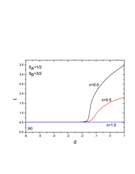
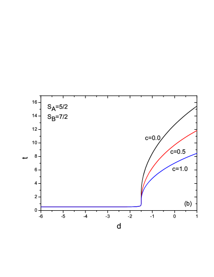
Figure 1: Variation of the critical temperature with crystal field parameter for selected values of the concentration $c=0.0$, $c=0.5$, $c=1.0$. Spin values of type-A and type-B atoms chosen as (a) $S_{A}=1/2$, $S_{B}=3/2$ and (b) $S_{A}=5/2$, $S_{B}=7/2$. Solid lines represent to the second order transitions.

4.2 Integer - Integer spin model

The second case of binary alloy system consists of both spin-A and spin-B with integer-integer values. In Fig. 2, the phase diagram in $(d,t)$ plane of the system is given for selected values of the concentrations $c=0.0$, $c=0.5$ and $c=1.0$. Spin values of the system have been chosen as $S_{A}=1$ $S_{B}=2$ in Fig 2 (a). We have examined only second order phase transition lines of phase diagram. The system exhibits tricritical point (TCP) as it passes from the second order phase transition to the first order phase transition. Behavior of the transition lines and reentrant phenomena in the presence of single-ion anisotropy is in agreement with the mixed spin-$1$ and spin-$2$ Ising system [28]. As seen in Figs. 2(a) and (b), TCP decreases as the concentration of type-A atoms increases. When the crystal field parameter takes large negative values, disordered phase appears for ground state, which consist of mostly occupied $s=0$ states, for all concentrations. If we fixed the spin value of A atoms as $S_{A}=1$ and then increase spin value of B atoms such as $S_{B}=3$, then the critical temperatures also increases as the concentration of B atoms increases for the positive crystal field parameter values ( compare Figs. 2 (a) and (b)). Besides it can be seen from Fig. 2 (b) that, TCP increases as the concentration goes towards zero, as in the case of $S_{A}=1,S_{B}=2$.

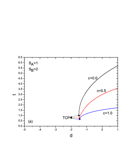
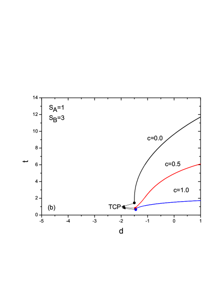
Figure 2: Variation of the critical temperature with crystal field parameter for selected values of the concentration $c=0.0$, $c=0.5$, $c=1.0$. Spin values of type-A and type-B atoms are chosen as (a) $S_{A}=1$, $S_{B}=2$ and (b) $S_{A}=1$, $S_{B}=3$. Solid lines represent the second order transitions. In figure, TCP stands for the tricritical point.

4.3 Integer - Half integer spin model

There are significantly noteworthy results for integer-half integer spin model. If we choose spin value of A atoms integer and spin value of B atoms half-integer, we obtain different results from the previous cases. We depict the phase diagrams in Fig. 3 corresponding to (a) $S_{A}=1$ $S_{B}=3/2$, (b) $S_{A}=1$ $S_{B}=7/2$ and (c) $S_{A}=2$ $S_{B}=5/2$ spin models. As we can see from Fig. 3 the system exhibits half integer spin valued phase diagram for $c=0$ and integer spin valued phase diagram behavior for $c=1$, as expected. Due to the fact that spin value of B atoms greater than the spin value of A atoms, as $c$ decreases, the critical temperatures rises. We can see from Fig 3 (a), for the concentration values $c=0$ and $c=0.5$, the phase diagrams contain second order transition lines. The system exhibits tricritical point TCP for $c=1$ and ferromagnetic ordered phase destroyed at negative large values of $d$ at the ground state. We can say that, this model behaves like half integer spin valued phase diagram for $c=0.5$. The decline of all critical temperatures is valid for all crystal field values for $c=0.5$. Note that, the critical temperatures for $c=0.5$ and $c=1$ do not merge (like in Fig 1 (a)) when the system takes negative large crystal field values. If we fix the spin value of A atoms as $S_{A}=1$ and then increase spin value of B atoms such as $S_{B}=7/2$, then the critical temperatures also increases for the values lower than $c=1$, which can be seen in Fig 3 (b). If we increase the difference between the spin values of A and B atoms, critical lines gradually begin to move further apart from each other. This fact can be seen by comparing phase diagrams in Figs. 3 (a) and (b). So can we make a general inference for concentration? For which value of the concentration, binary alloy system behave like integer spin valued phase diagram? To answer these questions, we examined the variation of the critical temperature with the concentration values in detail. The phase diagram in $(c,t)$ plane for selected values of crystal field parameters $d=1$, $d=0$, $d=-1$, $d=-2$, $d=-3$, $d=-4$ and $d=-5$ can be seen in Fig. 4. These curves are constructed for (a) $S_{A}=1$ $S_{B}=3/2$, (b) $S_{A}=1$ $S_{B}=7/2$ and (c) $S_{A}=2$ $S_{B}=5/2$ spin models. Critical temperature values differ from each other at the limiting cases $c=0$ and $c=1$. When $c$ concentration value increases from 0 to 1, all critical temperatures decrease. The system exhibits ferromagnetic phase at low temperatures for all concentrations and exhibits paramagnetic phase at high temperatures for $d=1$, $d=0$, $d=-1$. If the crystal field parameter takes negative values, all critical temperatures decrease. The system exhibits only second order phase transition lines for selected values of $d$. It is important to emphasize that when the crystal field takes negative large values, the concentration value which is the border between the ordered and disordered phase at ground state are the same. This critical concentration value is $c^{*}=0.74$ which can be seen in Figs. 4 (a), (b) and (c). When majority of the spins takes integer values, ground state changes from $s_{B}=\pm 1/2$ states to $s_{A}=0$ state. Therefore, phase transition occurs at $c^{*}=0.74$ for $d\rightarrow-\infty$ and it exhibits disordered phase for values greater than this value. If we fix the spin value of A atoms as $S_{A}=1$ and then increase spin value of B atoms such as $S_{B}=7/2$, then the critical temperatures also increases as $c$ goes towards zero (see Fig 4 (b)). No matter how big the difference between these spin values is, the critical concentration value is again $c^{*}=0.74$. As seen in Fig 4 (c), again the critical concentration value is $c^{*}=0.74$ for $S_{A}=2$ $S_{B}=5/2$ spin model. We have also performed calculations for other possible pairs of integer - half integer spin models, such that $S_{A}<S_{B}$, and we obtain exactly same result. $c^{*}=0.74$ value is obtained for all cases.

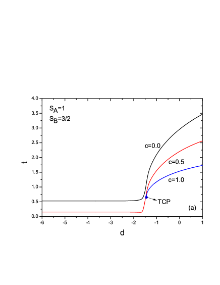
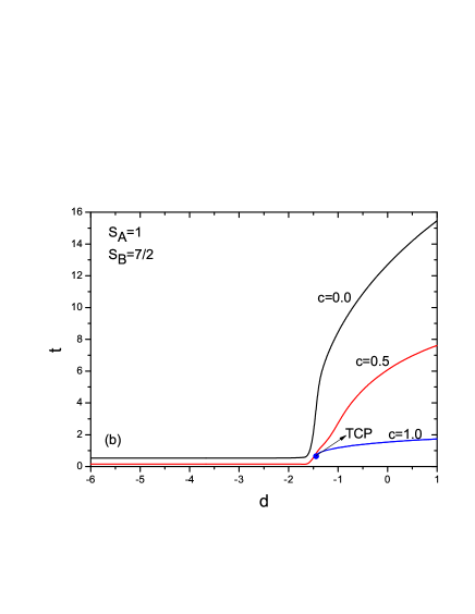
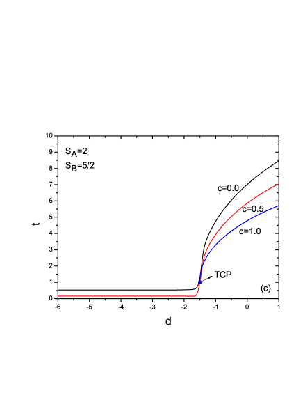
Figure 3: Variation of the critical temperature with crystal field parameter for selected values of the concentration $c=0.0$, $c=0.5$, $c=1.0$. Spin values of type-A and type-B atoms are chosen as (a) $S_{A}=1$, $S_{B}=3/2$, (b) $S_{A}=1$, $S_{B}=7/2$ and (c) $S_{A}=2$, $S_{B}=5/2$. Solid lines represent the second order transitions. In figure, TCP stands for the tricritical point.

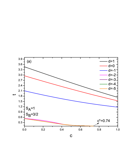
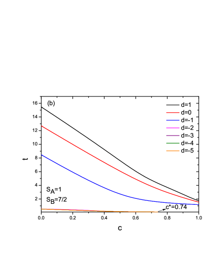
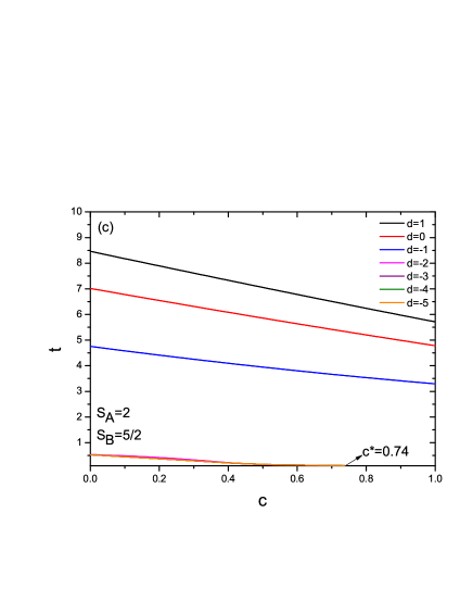
Figure 4: Variation of the critical temperature with the concentration for selected values of crystal field parameters $d=-1$, $d=-2$, $d=-3$, $d=-4$, $d=-5$. Spin values of type-A and type-B atoms chosen as (a) $S_{A}=1$, $S_{B}=3/2$, (b) $S_{A}=1$, $S_{B}=7/2$ and (c) $S_{A}=2$, $S_{B}=5/2$. Solid lines represent to the second order transitions.

4.4 Half integer - Integer spin model

Although it seems that this subsection is the same as previous subsection, indeed this case is different from the previous one due to $S_{A}<S_{B}$. We depict the phase diagrams of (a) $S_{A}=1/2$ $S_{B}=1$, (b) $S_{A}=3/2$ $S_{B}=2$ and (c) $S_{A}=3/2$ $S_{B}=3$ spin models, in Fig. 5. As seen in Fig 5 (a), the critical temperatures of the system will not change along the crystal field plane for $c=1$, due to the fact that, all spins has the value of $1/2$. The ordered ferromagnetic phase area resides below this temperature. As long as the system contributes to concentration from the B atoms, ordered phase area expands to the higher temperatures for the large values of crystal field parameter. Conversely, critical temperature decreases as the crystal field parameter takes negative large values. If the majority of concentration consists of integer spin model, ordered phase is destroyed under the influence of the negative large crystal field parameters. The second order phase transitions turn into the first order transitions, and the system displays a TCP. Topology of the phase diagrams is analogous to the integer-half integer binary alloy models [50, 51, 52]. If we choose spin values of the system as $S_{A}=3/2$, $S_{B}=2$ (Fig 5 (b)), the critical temperature increases for larger values of crystal field, whereas it decreases for negative large crystal field parameters. When all of the lattice sites consist of type-B atoms it displays a larger TCP value (compare Fig 5 (a) and (b)). In figure 5 (c), selected spin values are $S_{A}=3/2$, $S_{B}=3$. For higher spin models, if we fix the spin value of A atoms as $S_{A}=3/2$ and then increase spin value of B atoms such as $S_{B}=3$, both the critical temperatures and TCP increases for positive values of $d$. We will ask the first question that comes to our mind. Does the system have critical concentration value (as in the previous subsection) in the half integer-integer spin models? In order to generalize the results about the system, we investigate the behavior of the critical point in $(c,t)$ plane, for different crystal field parameter values. The phase diagram in $(c,t)$ plane for selected values of crystal field parameters $d=1$, $d=0$, $d=-1$, $d=-2$, $d=-3$, $d=-4$ and $d=-5$ can be seen in Fig. 6. The variation of the temperature with the concentration is constructed for (a) $S_{A}=1/2$, $S_{B}=1$, (b) $S_{A}=3/2$, $S_{B}=2$ and (c) $S_{A}=3/2$, $S_{B}=3$ half integer - integer spin models. In Fig. 6 (a) critical temperatures do not change according to the crystal field parameters for the system which has $c=1$ concentration. This is due to the spin value of $1/2$, which is not affected by crystal field. However, the type-B atoms are added to the system, the phase transition lines exhibit higher critical temperatures for large crystal field values, while the critical temperatures begin to decrease for negative large crystal field values. In other words, the ordered phase region increases for large crystal field values, while disordered phase appear for negative large crystal field values for the low concentration values. The critical concentration value is $c^{*}=0.26$ which yields border value between the ordered and disordered phase at ground state. When we start adding A atoms to the system, ground state changes from $s_{B}=0$ states to $s_{A}=\pm 1/2$ state. Therefore, phase transition occurs at $c^{*}=0.26$ for $d\rightarrow-\infty$ and it starts to exhibit ordered phase. Thus, we can say that the behavior of the integer spin-valued phase diagram is transformed into the half-integer spin-valued phase diagram after this critical value. In Fig. 6 (b) we select $S_{A}=3/2$, $S_{B}=2$ spin model. The system exhibits second order phase transitions for all crystal field parameters. Critical temperatures take different values at large values of crystal field parameter for $c=1$. Ferromagnetic phase area increases as the concentration value goes towards from $1$ to $0$ at positive crystal field parameters. The binary alloy model has paramagnetic phase area for the low concentrations, in the presence of the negative large crystal field. Critical concentration value appears at $c^{*}=0.26$. For higher order spin models, we select $S_{A}=3/2$, $S_{B}=3$ spin model that can be seen in Fig. 6 (c). As we increase the spin of the B atom, negative large crystal field causes the system drags to dragged into the disordered phase for low concentration values. Similarly, $c^{*}=0.26$ is also observed in Fig 6 (c). We have also performed further calculations for all half integer- integer spin models for cases of $S_{A}<S_{B}$ which will not be further included here but inspected. Therefore, the critical concentration value $c^{*}=0.26$ is valid for all half integer- integer spin models.

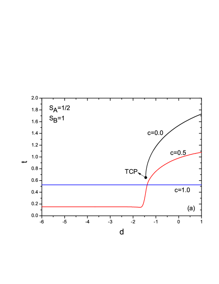
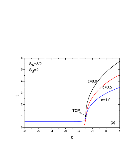
Figure 5: Variation of the critical temperature with crystal field parameter for selected values of the concentration $c=0.0$, $c=0.5$, $c=1.0$. Spin values of type-A and type-B atoms are chosen as (a) $S_{A}=1/2$, $S_{B}=1$, (b) $S_{A}=3/2$, $S_{B}=2$ and (c) $S_{A}=3/2$, $S_{B}=3$. Solid lines represent the second order transitions. TCP stands for the tricritical point.

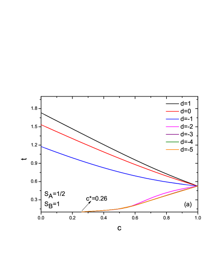
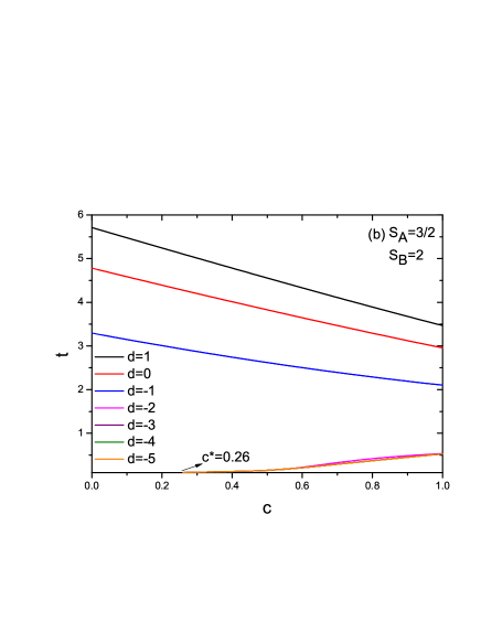
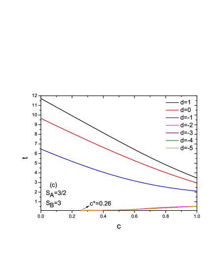
Figure 6: Variation of the critical temperature with the concentration for selected values of crystal field parameters $d=-1$, $d=-2$, $d=-3$, $d=-4$, $d=-5$. Spin values of type-A and type-B atoms are chosen as (a) $S_{A}=1/2$, $S_{B}=1$, (b) $S_{A}=3/2$, $S_{B}=2$ and (c) $S_{A}=3/2$, $S_{B}=3$. Solid lines represent the second order transitions.

5 Conclusion

In conclusion, we have investigated the critical properties of generalized spin-S magnetic binary alloys represented by $A_{c}B_{1-c}$ within the framework of EFT. The system consists of type-A and type-B atoms with the concentration $c$ and $1-c$ respectively. The evolution of the phase diagrams in $(d,t)$ and $(c,t)$ planes have been presented for selected values of the spins. We have obtained that different binary alloy models consisting of half integer or integer spin models has its specific phase diagram characteristic, as comparable with the literature [9, 22, 28, 48, 50].

For the binary alloy system which consist of only half integer spins, the system has an ordered phase in the ground state, regardless of the value of the crystal field. As expected, the ground state for large negative crystal field region, consists of occupied $\pm 1/2$ states. All phase diagrams of these systems consist of only second order critical points.

For the binary alloy system which consist of only integer spins, the system has disordered phase for large negative values of the crystal field. This disordered phase has ground state with filled $0$ states by the spins. Phase diagrams in $(d,t)$ plane exhibit tricritical point TCP. The presence of the TCP is the sign of the first order transitions. All of the phase diagrams have TCP regardless of the spin and concentration values, for this case.

Results of generalized spin-S binary alloy model has also been discussed as half integer-integer and integer- half integer spin models. We restrict our results in the case $S_{A}<S_{B}$. If the majority of the system consists of half-integer (integer) spin values, system exhibit ordered (disordered) phase at negative large crystal field values. The phase diagrams may display TCP according to the value of the concentration.

Another noteworthy point of our results is the presence of exactly the same critical concentration value that drives the system from paramagnetic to ferromagnetic phase, regardless of the spin values at large negative crystal field values. This value is $c^{*}=0.74$ for integer-half integer model and $c^{*}=0.26$ for half integer - integer model. Note that $(S_{A}<S_{B})$ is chosen. In other words, the integer-half integer binary system cannot have ordered phase for $c>0.74$, for large negative values of the crystal field. In the same manner the half integer-integer binary system cannot have ordered phase for $c>0.26$, for large negative values of the crystal field.

The physical explanation is as follows: when the majority of the lattice consists of integer spins, the ground state should be consists of occupied $0$ states. When the concentration rises in the integer-half integer case, this means that the number of integer spins rises. Ferromagnetic interactions between the spins tend the neighbor spins align along the same direction. This could create ordered phase. But, after some specific value of this concentration, ferromagnetic interactions cannot create ordered phase due to the rising concentration of occupied $0$ states.

We hope that the results obtained in this work may be beneficial form both theoretical and experimental point of view.

References

- [1] M. Blume, Phys. Rev. 141 (1966) 517.
- [2] H.W. Capel, Physica 32 (1966) 966.
- [3] J.A. Plascak, J.G. Moreira, F.C. sáBarreto, Phys. Lett. A 173 (1993) 360.
- [4] S.K. Ghatak and D. Sherrington, Journal of Physics C:Solid State Physics 10 (1977) 3149.
- [5] T. Kaneyoshi, J.W. Tucker and M. Jascur, Physica A 186 (1992) 495-512.
- [6] T. Kaneyoshi, Acta Physica Polonica A 83/6 (1993) 703.
- [7] E. Costabile, J. R. Viana, J. Ricardo de Sousa, J.A. Plascak, Physica A 393 (2014) 297-303.
- [8] Ü. Akıncı, Y. Yüksel, E. Vatansever, Phys. Lett. A 382 (2018) 3238-3243.
- [9] Ü. Akıncı, Physica A 483 (2017) 130-138.
- [10] J.W. Tucker, M. Saber and L. Peliti, Physica A 206 (1994) 497-507.
- [11] T. Kaneyoshi and M. Jascur, Physical Review B 48/1 (1993) 250.
- [12] Ü. Akıncı, Journal of Magnetism and Magnetic Materials 488 (2019) 165368.
- [13] D.P. Lara, J.A. Plascak, S.J. Ferreira et al., Journal of Magnetism and Magnetic Materials 177-181 (1998) 163.
- [14] O. Nagai, S. Miyashita, T. Horiguchi, Physical Review B 47/1 (1993) 202.
- [15] P.F. Fox and A.J. Guttmann, Journal of Physics C: Solid State Physics 6 (1973) 913.
- [16] W.J. Camp and J.P. Van Dyke, Physical Review B 11/7 (1975) 2579.
- [17] D.P. Lara, J.A. Plascak, Physica A 260 (1998) 443.
- [18] Y.Q. Wang and Z.Y. Li, Phys. Stat. Sol. (b) 189 (1995) 521.
- [19] A. Bobák, M. Jurcisin, Journal of Magnetism and Magnetic Materials 163 (1996) 292-298.
- [20] G.Z. Wei, Y.Q. Liang, Q. Zhang, Z.H. Xin, Journal of magnetism and magnetic materials 271(2-3) (2004) 246-253.
- [21] Y.Q. Liang, G.Z. Wei and G.L. Song, Phys. Stat. Sol. (b) 245/11 (2008) 2586-2592.
- [22] B. Deviren, M. Keskin and O. Canko, Physica A 388 (2009) 1835-1848.
- [23] T. Bahlagui, H. Bouda, A. El Kenz, L. Bahmad, A. Benyoussef, Superlattices and Microstructures 110 (2017) 90-97.
- [24] N. De La Espriella and G. M. Buendía, J. Phys.:Condens. Matter 23 (2011) 176003.
- [25] J. A. Reyes, N. De La Espriella, G. M. Buendıía, Phys. Status Solidi B 252/10 (2015) 2268-2274.
- [26] E. Albayrak, A. Yigit, Physics Letters A 353 (2006) 121–129.
- [27] H.K. Mohamad, H.F. Alturki, Journal of Superconductivity and Novel Magnetism 32/12 (2019) 3971-3978.
- [28] G. Wei, Y. Gu and J. Liu, Physical Review B 74 (2006) 024422.
- [29] O.F. Abubrig, D. Horv1áth, A. Bobák, M. Jascur, Physica A 296 (2001) 437– 450.
- [30] J.S. da Cruz Filho, M. Godoy, A.S. de Arruda, Physica A 392 (2013) 6247–6254.
- [31] A. Bobák, Physica A 286 (2000) 531–540.
- [32] M. Godoy, W. Figueiredo, International Journal of Modern Physics C, 20/1 (2009) 47-58.
- [33] T. Kaneyoshi, Journal of Magnetism and Magnetic Materials 151 (1995) 45-53.
- [34] B.Y. Yousif and R.G. Bowers, Journal of Physics A: Math. Gen. 17 (1984) 3389-3394.
- [35] Kun-Fa Tang, Journal of Physics A: Math. Gen. 21 (1988) L1097.
- [36] J. Strecka, Physica A 360 (2006) 379–390.
- [37] S. Matasovkská, M. Jascur, Physica A 383 (2007) 339–350.
- [38] J. Strecka, J. Dely, L. Canová, Physica A 388 (2009) 2394-2402.
- [39] G.J.A. Hunter, R.C.L. Jenkins and C.J. Tinsley, J. Phys. A: Math. Gen. 23 (1990) 4547-4551.
- [40] R. Honmura, A.F. Khater, I.P. Fittipaldi and T. Kaneyoshi, Solid State Communications, 41/5 (1982) 385-388.
- [41] T. Kaneyoshi, Z.Y. Li, Physical Review B, 35/4 (1987) 1869.
- [42] P.D. Shelton, Physical Review B, 32/1 (1985) 345.
- [43] J.L. Morán López and L.M. Falicov, Journal of Physics C: Solid State Physics, 13/9 (1980) 1715.
- [44] F. Mejía-Lira, Jesús Urias and J.L. Morán López, Physical Review B, 24/9 (1981) 5270.
- [45] M.F. Thorpe and A.R. McGurn, Physical Review B, 20/5 (1979) 2142.
- [46] T. Kaneyoshi, Journal of Physical Society of Japan, 55/5 (1986) 1430.
- [47] T. Kaneyoshi, Physical Review B, 33/11 (1986) 7688.
- [48] T. Kaneyoshi, Physical Review B, 34/11 (1986) 7866.
- [49] T. Kaneyoshi, Physical Review B, 39/16 (1989) 12134.
- [50] Ü. Akıncı, G. Karakoyun, Physica B: Condensed Matter 521 (2017) 365.
- [51] G. Karakoyun, Ü. Akıncı, Physica A: Statistical Mechanics and its Applications 510 (2018) 407.
- [52] G. Karakoyun, Ü. Akıncı, Physica B: Physics of Condensed Matter 578 (2020) 411870.
- [53] J.A. Plascak, Physica A 198 (1993) 655.
- [54] D.G. Rancourt, M. Dubé and P.R.L. Heron, Journal of Magnetism and Magnetic Materials 125 (1993) 39.
- [55] T. Kawasaki, Progress of Theoretical Physics, 58/5 (1977) 1357.
- [56] D.S. Cambuí, A.S. De Arruda and M. Godoy, International Journal of Modern Physics C, 23/08 (2012) 1240015.
- [57] T. Kaneyoshi, Journal of Physics: Condensed Matter 5/40 (1993) L501.
- [58] T. Kaneyoshi and M. Jascur, Journal of Physics: Condensed Matter 5/19 (1993) 3253.
- [59] T. Kaneyoshi, Physica B, 193 (1994) 255-264.
- [60] M. Jascur and T. Kaneyoshi, Physica A 220 (1995) 542-551.
- [61] T. Kaneyoshi and M. Jascur, Physica A 203 (1994) 316-327.
- [62] T. Kaneyoshi, Physica B 210 (1995)178-182.
- [63] A.I. Lukanin, M.V. Medvedev, physica status solidi (b), 121/2 (1984) 573-582.
- [64] J. Dely, A. Bobák, Journal of Magnetism and Magnetic Materials 305 (2006) 464-466.
- [65] M. Źuković, A. Bobák, Journal of Magnetism and Magnetic Materials 322 (2010) 2868-2873.
- [66] Y. Yüksel, Ü. Akıncı, Journal of Physics and Chemistry of Solids 112 (2018) 143-152.
- [67] A.S. Freitas, D.F. de Albuquerque, N.O. Moreno, Physica A 391 (2012) 6332-6336.
- [68] G.A. Pérez Alcazar, J.A. Plascak and E. Galváo da Silva, Physical Review B 34/3 (1986) 1940.
- [69] A.S. Freitas, D.F. de Albuquerque, N.O. Moreno, Journal of Magnetism and Magnetic Materials 361 (2014) 137-139.
- [70] A.S. Freitas, D.F. de Albuquerque, Solid State Communications, 225 (2016) 44-47.
- [71] D.P. Lara, G.A. Pérez Alcazar, L.E. Zamora, J.A. Plascak, Physical Review B 80 (2009) 014427.
- [72] M. C. Cadeville and J.L. Morán López, Physics Reports 153/6 (1987) 331-399.
- [73] M.A. Kobeissi, Journal of Physics: Condensed Matter 3 (1991) 4983-4998.
- [74] K. Adachi, K. Sato and M. Takeda, Journal of Physical Society of Japan, 26/3 (1969) 631.
- [75] K. Fukamichi, M. Kikuchi, S. Arakawa and T. Masumoto, Solid State Communications, 23 (1977) 955.
- [76] S.A. Nikitin and N.P. Arutyunian, Zh. Eksp. Teor. Fiz, 77 (1979) 2018-2027.
- [77] F. C. SáBarreto, I. P. Fittipaldi, B. Zeks, Ferroelectrics 39 (1981) 1103.
- [78] J. Strecka, M. Jascur, acta physica slovaca 65 (2015) 235.
- [79] R. Honmura, T. Kaneyoshi, J. Phys. C: Solid State Phys. 12 (1979) 3979.
- [80] T. Kaneyoshi, J. Tucker, M. Jascur, Physica A 176, 495 (1992).