Regularization of systems of nonlinear ill-posed equations: II. Applications

Abstract

In part I we introduced modified Landweber–Kaczmarz methods and have established a convergence analysis. In the present work we investigate three applications: an inverse problem related to thermoacoustic tomography, a nonlinear inverse problem for semiconductor equations, and a nonlinear problem in Schlieren tomography. Each application is considered in the framework established in the previous part. The novel algorithms show robustness, stability, computational efficiency and high accuracy.

Markus Haltmeier

Department of Computer Science, University of Innsbruck

Technikerstr. 21a, A-6020 Innsbruck, Austria

Richard Kowar

Department of Computer Science, University of Innsbruck

Technikerstr. 21a, A-6020 Innsbruck, Austria

Antonio Leitão

Department of Mathematics, Federal University of St. Catarina

P.O. Box 476, 88040-900 Florianópolis, Brazil

Otmar Scherzer

Department of Computer Science, University of Innsbruck

Technikerstr. 21a, A-6020 Innsbruck, Austria,

and

RICAM, Austrian Academy of Sciences

Altenberger Straße 69, A-4040 Linz, Austria.

2000 Mathematics Subject Classification. Primary: 65J20, 65J15; Secondary: 47J06.
Keywords. Ill-posed systems; Landweber–Kaczmarz methods; Inverse doping; Schlieren tomography; Thermoacoustic tomography.

1 Introduction

In [8] we analyzed novel iterative Landweber–Kaczmarz methods for solving systems of ill-posed equations

$$\mathrm{F}_{i}(x)=y^{\delta,i}\,,\quad\;i=0,\dots,N-1\;.$$ (1)

Here $\mathrm{F}_{i}:D_{i}\subseteq X\to Y$ are operators between Hilbert spaces $X$ and $Y$ and $y^{\delta,i}$ are approximations of noise free data $y^{i}$ with $\|y^{\delta,i}-y^{i}\|\leq\delta^{i}$ for $i\in\{0,\dots,N-1\}$.

The first method analyzed in [8] is the loping Landweber–Kaczmarz (lLK) method

$$x_{n+1}=x_{n}-\omega_{n}{\mathrm{F}_{[n]}^{\prime}(x_{n})}^{\ast}(\mathrm{F}_{[n]}(x_{n})-y^{\delta,[n]})\,,$$ (2)

with a bang–bang relaxation parameter

$$\omega_{n}:=\omega_{n}(\delta^{i},y^{\delta,i})=\begin{cases}1&\|\mathrm{F}_{[n]}(x_{n})-y^{\delta,i}\|>\tau\delta^{i}\\ 0&\mbox{ otherwise}\end{cases}\,.$$ (3)

Here $\tau>2$ is an appropriately chosen constant and $[n]:=n\mod N$. We refer to $N$ subsequent iterations as one iteration cycle. The lLK method skips inner iterations, if the data are sufficiently well approximated. The whole iteration is terminated if $\|\mathrm{F}_{i}(x_{n_{\ast}^{\delta}+i})-y^{\delta,i}\|<\tau\delta^{i}$ for all $i\in\{0,\dots,N-1\}$.

The second method analyzed in [8], is the embedded Landweber–Kaczmarz (eLK) method,

$$\mathbf{x}_{n+1/2} =\mathbf{x}_{n}-\omega_{n}\mathbf{F}^{\prime}(\mathbf{x}_{n})^{\ast}(\mathbf{F}(\mathbf{x}_{n})-\mathbf{y}^{\delta})\,,$$ (4)

$$\mathbf{x}_{n+1} =\mathbf{x}_{n+1/2}-\omega_{n+1/2}\mathbf{G}(\mathbf{x}_{n+1/2})\,.$$ (5)

Here $\mathbf{x}:=(x^{i})_{i}\in X^{N}$, $\mathbf{y}^{\delta}:=(y^{\delta,i})_{i}\in Y^{N}$, $\mathbf{F}(\mathbf{x}):=(\mathrm{F}_{i}(x^{i}))_{i}\in Y^{N}$, $\delta:=\max\{\delta^{i}:i=0,\dots,N-1\}$ and $\mathbf{G}$ is a scalar multiple of the steepest descent direction of the functional $\mathcal{G}(\mathbf{x}):=\sum_{i=0}^{N-1}\|x^{i+1}-x^{i}\|^{2}$ on $X^{N}$. Moreover,

$$\begin{aligned} \omega_{n}&=\begin{cases}1&\|\mathbf{F}(\mathbf{x}_{n})-\mathbf{y}^{\delta}\|>\tau\delta\\ 0&\mbox{ otherwise }\end{cases}\,,\\ \omega_{n+1/2}&=\begin{cases}1&\|\mathbf{G}(\mathbf{x}_{n+1/2})\|>\tau\epsilon(\delta)\\ 0&\mbox{ otherwise }\end{cases}\,,\end{aligned}$$

with $\epsilon(\delta)\to 0$, as $\delta\to 0$. The eLK iteration is terminated after $n_{\star}^{\delta}$ iterations when $\|\mathbf{F}(\mathbf{x}_{n_{\star}^{\delta}})-\mathbf{y}^{\delta}\|\leq\tau\delta$ and $\|\mathbf{G}(\mathbf{x}_{n_{\star}^{\delta}})\|\leq\tau\epsilon(\delta)$. One cycle of the eLK method is defined by performing both iterations in (4) and (5). Motivations for these iteration methods can be found in [8].

In [8] we have proven stability and convergence for both the eLK and lLK method. In this article we apply the methods to three different problems: a linear inverse problem related to thermoacoustic tomography, an inverse problem for semiconductors and Schlieren tomography. For validation, the results are compared to the classical Landweber–Kaczmarz (LK) method [18, 11]

$$x_{n+1}=x_{n}-\mathrm{F}_{[n]}^{\prime}(x_{n})^{\ast}(\mathrm{F}_{[n]}(x_{n})-y^{\delta,[n]})\,.$$ (6)

The outline of this article is as follows. In Section 2 we apply both methods, the lLK method and the eLK method, to an inverse problem related to thermoacoustic computed tomography, which mathematically can be reduced to the inversion of the circular mean transform. In Section 3 we consider the exponentially ill-posed nonlinear inverse problem of estimating the doping profile in a semiconductor from voltage–current measurements. In Section 4 we consider Schlieren tomography, an imaging method for reconstructing three dimensional pressure fields.

2 Thermoacoustic computed tomography

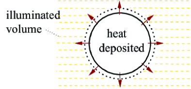
Thermoacoustic computed tomography is a promising new imaging modality that has the potential to become a mayor non–invasive imaging method. In thermoacoustic imaging an object of interest is illuminated by short electromagnetic pulses, such as optical illumination or radio waves, which results in an excitation of acoustic waves (pressure variations). The spatially varying initial pressure distribution inside the object caries valuable structural and functional information and is reconstructed from acoustical data which is recorded with detectors outside of the object. Among the several publications on thermoacoustic imaging we mention [2, 12, 22, 23, 24].

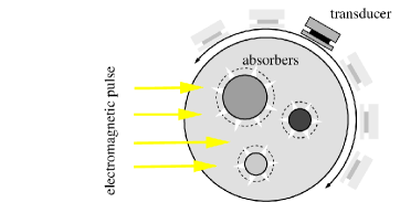
Figure 1: Thermoacoustic computed tomography. Left. A sample is illuminated with pulsed electromagnetic energy. Right. The induced acoustic waves are recorded with acoustic detectors located outside of the object.

2.1 Mathematical model

Assume that the initial pressure distribution $x(\xi_{1},\xi_{2})$ is independent of the third spatial coordinate, let $\boldsymbol{\xi}:=(\xi_{1},\xi_{2})$ and let $B_{R}$ denote the open disc (in $\mathbb{R}^{2}$) with radius $R$.

Mathematically, in such a situation, thermoacoustic tomography reduces to the problem of recovering $x$ from [9]

$$\mathrm{M}_{i}(x)=y^{\delta,i}\,,\quad i=0,\dots,N-1.$$ (7)

with noisy data $y^{\delta,i}$, where

$$\mathrm{M}_{i}(x)(t):=\frac{1}{\sqrt{\pi}}\int_{S^{1}}x(\boldsymbol{\xi}_{i}+t\boldsymbol{\sigma})\,\mathrm{d}\Omega(\boldsymbol{\sigma})\,,\quad i=0,\dots,N-1$$ (8)

is the scaled mean value of $x\in C_{0}^{\infty}(B_{R})$ over the circle with center $\boldsymbol{\xi}_{i}\in\partial B_{R}$ and radius $t\in[0,2R]$. Here $S^{1}$ denotes the surface of the unit disc in $\mathbb{R}^{2}$ and $\mathrm{d}\Omega$ the line measure on $S^{1}$ and $(\boldsymbol{\xi},0)$ corresponds to the locations of an acoustic receiver, see Figure 1. This section is devoted to the stable solution of (7).

Recently, we proposed a detection technique [5] where an array of parallel line detectors is rotated around the around the object and pressure signals along the line detectors are recorded. Then the solution of (7) allows for reconstructing of a fully three dimensional initial pressure distribution. In experiments line detectors are realized by thin laser beams that are either part of a Fabry–Perot or a Mach–Zehnder interferometer [5, 19].

2.2 Abstract formulation in Hilbert–spaces

In the following we show that the problem of recovering of a function $x$ from its circular means can be put in the abstract framework of [8].

In the remainder of this section, let $L^{2}(B_{R})$ be the Hilbert space of square integrable functions on $B_{R}$ with $\|x\|^{2}:=\int_{B_{R}}x(\boldsymbol{\xi})^{2}d\boldsymbol{\xi}$. Moreover, we denote by $L^{2}([0,2R],t\mathrm{d}t)$ the Hilbert space of all functions $y:[0,\infty)\to\mathbb{R}$ (observable quantities) with support in $[0,2R]$ with

$$\|y\|_{Y}^{2}:=\int_{0}^{\infty}y(t)^{2}\,t\mathrm{d}t<\infty\,.$$

Finally we denote by

$$\langle y_{1},y_{2}\rangle_{Y}=\int_{0}^{\infty}y_{1}(t)y_{2}(t)\,t\mathrm{d}t$$

the associated inner product on $L^{2}([0,2R],t\mathrm{d}t)$.

The scaled circular mean operators are defined by

$$\mathrm{M}_{i}:C_{0}^{\infty}(B_{R})\to L^{2}([0,2R],t\mathrm{d}t):x\mapsto\mathrm{M}_{i}(x)\,,$$

where $\mathrm{M}_{i}(x)$ is defined by (8).

Theorem 1.

The operators $\mathrm{M}_{i}$ can be continuously extended to $\mathrm{M}_{i}:L^{2}(B_{R})\to L^{2}([0,2R],t\mathrm{d}t)$ with $\|\mathrm{M}_{i}\|\leq 1$. The adjoint $\mathrm{M}_{i}^{\ast}:L^{2}([0,2R],t\mathrm{d}t)\to L^{2}(B_{R})$ is given by

$$\mathrm{M}_{i}^{\ast}(y)(\boldsymbol{\xi})=y(|\boldsymbol{\xi}_{i}-\boldsymbol{\xi}|)/\sqrt{\pi}\,,\quad\;i=0,\dots,N-1\;.$$ (9)

Proof.

Assume that $x\in C_{0}^{\infty}(B_{R})$. From the definition of $\mathrm{M}_{i}(x)$, the Cauchy Schwarz inequality and Fubini’s theorem it follows that

$$\|\mathrm{M}_{i}(x)\|_{Y}^{2} =\frac{1}{\pi}\int_{0}^{\infty}\left(\int_{S^{1}}x(\boldsymbol{\xi}_{i}+t\boldsymbol{\sigma})\cdot\chi_{B_{R}}(\boldsymbol{\xi}_{i}+t\boldsymbol{\sigma})\,\mathrm{d}\Omega(\boldsymbol{\sigma})\right)^{2}t\mathrm{d}t$$

$$\leq\frac{1}{\pi}\int_{0}^{\infty}\left(\int_{S^{1}}\chi_{B_{R}}(\boldsymbol{\xi}_{i}+t\boldsymbol{\sigma})\,\mathrm{d}\Omega(\boldsymbol{\sigma})\int_{S^{1}}x(\boldsymbol{\xi}_{i}+t\boldsymbol{\sigma})^{2}\,\mathrm{d}\Omega(\boldsymbol{\sigma})\right)t\mathrm{d}t$$

$$\leq\int_{0}^{\infty}\int_{S^{1}}x(\boldsymbol{\xi}_{i}+t\boldsymbol{\sigma})^{2}\ \mathrm{d}\Omega(\boldsymbol{\sigma})\ t\mathrm{d}t=\|x\|^{2}\,.$$

Hence $\mathrm{M}_{i}$ is bounded from $C_{0}^{\infty}(\Omega)$ into $L^{2}([0,2R],tdt)$ and therefore can be extended to a bounded linear operator mapping on $L^{2}(B_{R})$ with $\|\mathrm{M}_{i}\|\leq 1$. In particular $\mathrm{M}_{i}$ has a bounded adjoint.

Let $x\in C_{0}^{\infty}(B_{R})$ and $y\in C_{0}^{\infty}([0,2R])$. From Fubini’s theorem and the substitution $\boldsymbol{\xi}=\boldsymbol{\xi}_{i}+t\boldsymbol{\sigma}$ it follows that

$$\langle\mathrm{M}_{i}(x),y\rangle_{Y} =\frac{1}{\sqrt{\pi}}\int_{0}^{\infty}y(t)\left(\int_{S^{1}}x(\boldsymbol{\xi}_{i}+t\boldsymbol{\sigma})\,\mathrm{d}\Omega(\boldsymbol{\sigma})\right)t\mathrm{d}t$$

$$=\frac{1}{\sqrt{\pi}}\int_{S^{1}}\int_{0}^{\infty}x(\boldsymbol{\xi}_{i}+t\boldsymbol{\sigma})y(t)\,t\mathrm{d}t\,\mathrm{d}\Omega(\boldsymbol{\sigma})$$

$$=\int_{B_{R}}x(\boldsymbol{\xi})\frac{y(|\boldsymbol{\xi}-\boldsymbol{\xi}_{i}|)}{\sqrt{\pi}}\,\mathrm{d}\boldsymbol{\xi}=\langle x,\mathrm{M}_{i}^{\ast}(y)\rangle\,.$$

This shows (9). ∎

We note that, for linear bounded operators, the tangential cone condition [8, Eq. (15)] is satisfied with $\eta=0$. Since $\mathrm{M}_{i}$ is linear and $\|\mathrm{M}_{i}\|\leq 1$, the lLK method and the eLK method provide convergent regularization methods for solving (7).

2.3 Numerical reconstruction

The lLK method applied to thermoacoustic computed tomography reads as

$$x_{n+1}=x_{n}-\omega_{n}\mathrm{M}_{[n]}^{\ast}(\mathrm{M}_{[n]}(x_{n})-y^{\delta,[n]})\,,$$ (10)

with

$$\omega_{n}=\omega_{n}(\delta,y^{\delta})=\begin{cases}1&\|\mathrm{M}_{[n]}(x)-y^{[n],\delta}\|>\tau\delta^{[n]}\\ 0&\mbox{ otherwise }\end{cases}\,.$$ (11)

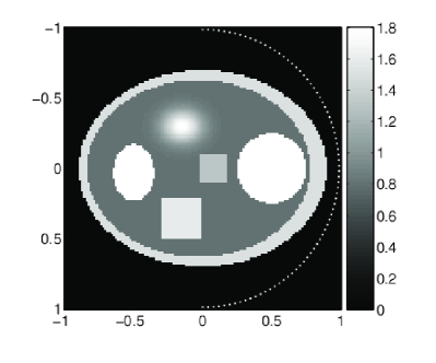
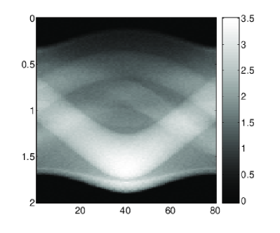
Figure 2: The left picture shows the phantom to be reconstructed, where the white dots indicate the locations of the detectors. The corresponding data $(\mathrm{M}_{i}(x))_{i}$ is depicted in the right image.

In the numerical implementation the spaces $L^{2}(B_{R})$ and $L^{2}([0,2R],t\mathrm{d}t)$ are approximated by the linear spans of piecewise linear splines. Each spline is represented by vectors in $\mathbb{R}^{M\times M}$ and $\mathbb{R}^{M}$, respectively. For the numerical evaluation of $\mathrm{M}_{i}$ the integration over $S^{1}$ in (8) is performed with the trapezoidal quadrature formula. This requires $\mathcal{O}(M)$ floating point operations (FLOPS) for any radius. Therefore, one iteration in the eLK method according to (10), (11) requires $\mathcal{O}(M^{2})$ FLOPS. In thermoacoustic tomography $M=\mathcal{O}(N)$, and the numerical effort for performing a complete Landweber–Kaczmarz cycle is $\mathcal{O}(N^{3})$. This is the same complexity that is needed to perform one step in the Landweber iteration.

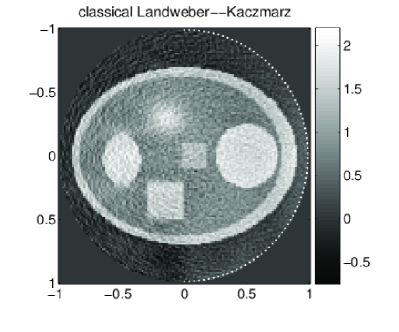
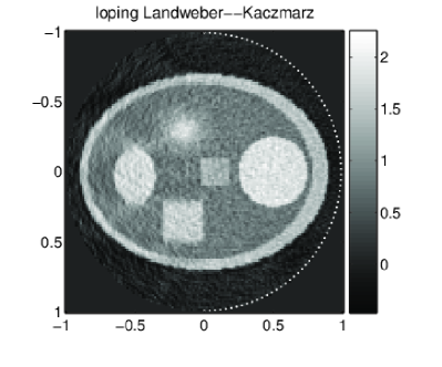
Figure 3: Numerical reconstruction of the phantom depicted in Figure 2. The left picture shows the regularized solution $x_{n^{\ast}_{\delta}}$ with the lLK method (10), (11). The right picture shows the reconstruction with the LK method using the same number of $n^{\ast}_{\delta}$ of iterations.

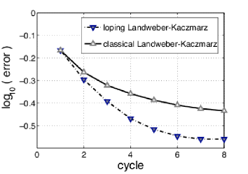
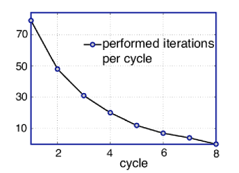
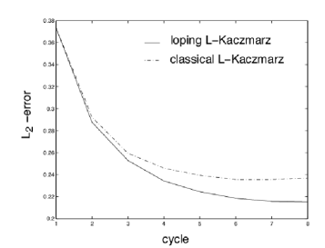
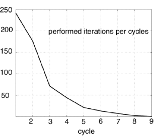
Figure 4: The left image shows the decrease of the error using the lLK method (10), (11) and the LK method. The right picture shows the actually performed number of iterations within a cycle of the lLK method. Within the $8$–th cycle all $\omega_{n}=0$ and the iteration terminates.

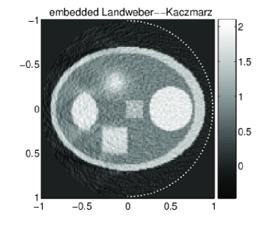
In the following numerical examples we consider $N=80$ measurements, where the centers $\xi_{i}=R(\sin(\pi i/N)\cos(\pi i/N))$ are uniformly distributed on the semicircle $S^{+}:=\{(\xi_{1},\xi_{2})\in\partial B_{R}:\xi_{1}\geq 0\}$. The phantom $x$, shown in the right picture in Figure 2, consists of a superposition of characteristic functions and one Gaussian kernel. The data $\mathrm{M}_{i}(x)$ was calculated via numerical integration and $5\%$ uniformly distributed noise was added. Micro-local analysis predicts, that in such limited angle situation certain details of $x$ outside the convex hull of $S^{+}$ cannot be recovered in a stable way [16, 25]. The numerical reconstruction with the lLK method, implemented with $\tau=2.0$, is depicted in Figure 3. The stopping rule becomes active after 8 cycles. For comparison purposes, the result of the LK method is plotted after 8 cycles. Figure 5 shows results obtained with the eLK method using the same phantom. We remind that the iterates of the eLK method are vectors $\mathbf{x}_{n}=(x^{0}_{n},\dots x^{N-1}_{n})$. For the results depicted in Figure 5 we used the average $x_{n}:=\sum_{i=0}^{N-1}x^{i}_{n}$ over all components.

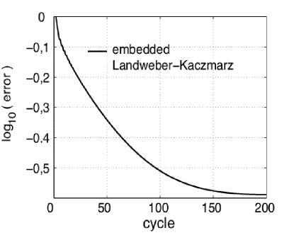
Figure 5: Numerical reconstruction of the phantom depicted in Figure 2 with the eLK method after 230 iterations (left) and decrease of the error (right).

2.4 Discussion

The left image in Figure 4 shows the decrease of error for both the LK method and the lLK method. The number of actually computed Landweber steps in the lLK method (number of iterations with $\omega_{n}=1$ within one cycle) of the lLK method is shown in the right image in Figure 4. The lLK method provides a better approximation of the exact solution than the LK method. Moreover, since more than half of the iterates are loped (see right picture in Figure 4), the numerical effort is remarkably smaller. Since in the eLK method an averaging over all components of the solution vector $\mathbf{x}_{n_{\star}^{\delta}}$ is performed, the quality of the reconstruction is slightly better than for the lLK method (and other tested regularization methods). Shortcoming of the eLK method are the larger amount of memory and the larger number of iteration cycles needed.

3 An inverse problem for semiconductors

In this section we investigate the solution of an inverse problem for nondestructive testing of semiconductors. More precisely, we aim to recover the doping profile on the basis of a simplified drift diffusion model from measurements given by the voltage–current (VC) map [15, 14].

The precise implantation of the doping profile is crucial for the desired performance of semiconductor devices in practice. In order to minimize manufacturing costs of semiconductors as well as for quality control, there is substantial interest in replacing expensive laboratory testing by numerical simulation for non–destructive evaluation.

3.1 Mathematical modelling

Let $\Omega\subset\mathbb{R}^{d}$, $d\in\{1,2,3\}$, be a domain representing the semiconductor device and let $\nu$ denote the unit normal vector to its boundary $\partial\Omega$. The boundary of $\Omega$ is divided into two nonempty disjoint parts $\partial\Omega_{N}$ and $\partial\Omega_{D}$. The Dirichlet part of the boundary $\partial\Omega_{D}$ models the Ohmic contacts, where an electrostatic potential is induced. The Neumann part of the boundary $\partial\Omega_{N}$ corresponds to insulating surfaces.

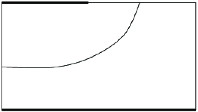
The doping profile $C:\Omega\to\mathbb{R}$ (unknown parameter) models the preconcentration of ions in the crystal, which is produced by diffusion of different materials into the silicon crystal and by implantation with an ion beam. In particular, $C=C_{+}-C_{-}$, where $C_{+}$ and $C_{-}$ are concentrations of positive and negative ions, respectively. In those subregions of $\Omega$ in which the preconcentration of negative ions predominate (P-region), we have $C<0$. Analogously, we define the N-region, where $C>0$. The boundaries between the P-regions and N-regions (where $C$ changes sign) are called the PN-junctions, see Figure 6.

Figure 6: P-N diode. Example of P-N junction.

We review the linearized stationary unipolar mathematical model, which is described by a drift diffusion equation (see [15, 14]):

$$\lambda^{2}\,\Delta V=\ e^{V}-C(\boldsymbol{\xi})\,,\quad \mbox{in}\ \Omega$$ (12)

$$V=\ V_{\rm bi}\,,\quad \mbox{on }\partial\Omega_{D}$$ (13)

$$\nabla V\cdot\nu=\ 0\,,\quad \mbox{on }\partial\Omega_{N}\,.$$ (14)

and

$$\nabla\cdot\left[\mu_{n}\,e^{V}\,\nabla u\right]=0\,,\quad \mbox{in }\Omega$$ (15)

$$u=U(\boldsymbol{\xi})\,,\quad \mbox{on }\partial\Omega_{D}$$ (16)

$$\nabla u\cdot\nu=0\,,\quad \mbox{on }\partial\Omega_{N}$$ (17)

Here, the function $V:\Omega\to\mathbb{R}$ denotes the electrostatic potential ($-\nabla V$ is the electric field) and $u:\Omega\to\mathbb{R}$ corresponds, up to an exponential transformation, to the concentration of free carriers of negative charge (the concentration of free positive charge is assumed to vanish; the reason why the model is called unipolar). The positive constant $\mu_{n}$ is related to the mobility of electrons and $\lambda^{2}$ is the Debye length.

At the Dirichlet part of the boundary $\partial\Omega_{D}$ the potential $V$ and the concentration $u$ are prescribed: $V_{\rm bi}$ is a given logarithmic function [14], and the function $U$ denotes the applied potential. At the the Neumann part of the boundary $\partial\Omega_{N}$ zero current flow (17) and a zero electric field in the normal direction (14) are prescribed.

In this section we are concerned with determining the inverse doping problem for the VC map, which consists in the determination of the doping profile $C$ in system (12–17) from measurements of the VC map

$$\Sigma_{C}: H^{3/2}(\partial\Omega_{D})\to\mathbb{R}\,$$

$$U\mapsto\Sigma_{C}(U):=\mu_{n}\int_{\Gamma_{1}}e^{V_{\rm bi}}\frac{\partial u}{\partial\nu}\,d\Gamma$$

which maps an applied potential $U$ at $\partial\Omega_{D}$ to the current flow $\Sigma_{C}(U)$ through the contact $\Gamma_{1}$. Here $(V,u)$ solve (12–17) and $\partial u/\partial\nu$ is the normal derivative of $u$. For results on existence and uniqueness of $H^{1}$-solutions of system (12–17), we refer to [15].

Since systems (12–14) and (15–17) are decoupled, we can split the inverse problem in two parts: First, the inverse problem of identifying the parameter $x(\boldsymbol{\xi}):=e^{V(\boldsymbol{\xi})}$ in (15–17) from measurements of the Dirichlet to Neumann (DN) map

$$\Lambda_{x}: H^{3/2}(\partial\Omega_{D})\to\mathbb{\mathbb{R}}$$ (18)

$$U\mapsto \Lambda_{x}(U):=\mu_{n}\int_{\Gamma_{1}}x\,\frac{\partial u}{\partial\nu}\,d\Gamma$$

is solved. The second step consists in the determination of the doping profile from (12), namely $C=x-\lambda^{2}\Delta(\ln x)$.

Notice that the second step is related to twice numerical differentiation which is mildly ill-posed (see [7]). On the other hand, the first step corresponds to the inverse problem of impedance tomography (EIT) with partial data, which is known to be severely ill-posed. (A review of EIT can be found in [3].) For the sake of clarity of presentation we will focus on the problem of identifying $x$ in the first step above.

3.2 Abstract formulation in Hilbert space

Due to the nature of the practical experiments, some restrictions on the data have to be taken into account:

1. The voltage profiles $U\in H^{3/2}(\partial\Omega_{D})$ must satisfy $U|_{\Gamma_{1}}=0$.

2. $x$ has to be determined from a finite number of measurements, i.e. from the given data

   $$F_{i}(x):=\Lambda_{x}(U_{i})\in Y:=\mathbb{R}\,,\quad i\in\{0,\dots,N-1\}\,,$$ (19)

   where $U_{i}\in H^{3/2}(\partial\Omega_{D})$ are prescribed voltage profiles satisfying $U_{i}|_{\Gamma_{1}}=0$.

         

(a)                                                      (b)

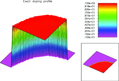
Figure 7: Picture (a) show the doping profile to be identified. Picture (b) shows a typical voltage profile $U_{j}$ and the corresponding solution $u$ of (15–17).

(a1)                                                      (b1)

(a2)                                                      (b2)

       

(a3)                                                            (c)

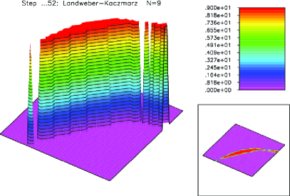
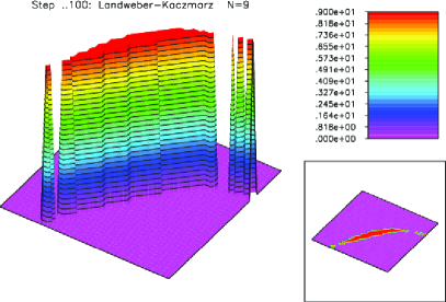
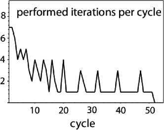
Figure 8: Numerical reconstruction of the p-n junction in Figure 7 (a). Pictures (a1–a3) show the decrease of the iteration error for the LK method. Pictures (b1, b2) show the corresponding evolution for the lLK method, and picture (c) the number of computed Landweber steps in each cycle of the lLK method.

In order to apply the abstract framework of [8] we write the inverse doping problem as a system of operator equations

$$\mathrm{F}_{i}(x)=y^{\delta,i}\,,\quad i=0,\dots,N-1\,.$$

Here $x\in L^{2}(\Omega)=:X$ is the unknown parameter, $y^{\delta,i}\in\mathbb{R}$ denotes measurement data and $\mathrm{F}_{i}:X\to Y$ are the parameter to output maps, with domain of definition

$$D(\mathrm{F}_{i}):=\{x\in L^{\infty}(\Omega):\,0<x_{\rm min}\leq x\leq x_{\rm max},\mbox{ a.e.}\}\,.$$

Although the operators $\mathrm{F}_{i}$ are Fréchet differentiable, they do not satisfy the tangential cone condition [8, Eq. (13)]. Therefore, the convergence results derived in [8, Section 2] cannot be applied.

3.3 Numerical reconstruction

In the following numerical examples we assume that $N=9$ Dirichlet–Neumann pairs $(U_{i},F_{i}(x))$ of measurement data are available. The domain $\Omega\subset\mathbb{R}^{2}$ is the unit square, and the boundary parts are defined as follows

$$\Gamma_{1} :=\{(s,1):\ s\in(0,1)\}\,,$$ (20)

$$\Gamma_{0} :=\{(s,0):\ s\in(0,1)\}\,,$$

$$\partial\Omega_{N} :=\{(0,t):\ t\in(0,1)\}\cup\{(1,t):\ t\in(0,1)\}\,.$$

The fixed inputs $U_{j}$, are chosen to be piecewise constant functions supported in $\Gamma_{0}$

$$U_{j}(s)\ :=\ \left\{\begin{array}[]{rl}1,&|s-s_{j}|\leq h\\ 0,&{\rm else}\end{array}\right.$$

where the points $s_{j}$ are uniformly distributed on $\Gamma_{0}$ and $h=1/32$. The doping profile to be reconstructed is shown in Figure  7 (a). In Figure 7 (b) a typical voltage profile $U_{j}$ (applied at $\Gamma_{0}$) is shown as well as the corresponding solution $u$ of (15–17). In these pictures, as well as in the forthcoming ones, $\Gamma_{1}$ appears on the lower left edge and $\Gamma_{0}$ on the top right edge (the origin corresponds to the upper right corner).

In Figure 8 we show the evolution of the iteration error for both the LK method (a1–a3) and the lLK method (b1, b2). The number of actually computed Landweber steps within each cycle of the lLK method is shown in Figure 8 (c).

The stopping rule for the lLK method with $\tau=2.0$ is satisfied after 52 cycles. In Figures 8 (b1, b2) one can see the iteration error after 10 and 52 cycles. For comparison purposes, the iteration error for the LK method is plotted in Figures 8 (a1–a3) after 10, 50 and 100 cycles.

3.4 Discussion

The LK method requires almost twice as much cycles as the lLK method in order to obtain a similar accuracy. The efficiency of the lLK method becomes even more evident when we compare the total number of actually performed iterations. Each cycle of the LK method requires the computation of 9 iterations, while in the lLK method the number of actually performed iterations is very small after a few iteration cycles. As one can see in Figure 8 (c), no more than 3 Landweber steps are computed after the $20$–th cycle of the lLK method. In total for the computation of the approximation in Figure 8 (a3), 900 iterations are needed, while the approximation in (b2) requires the computation of only 146 iterations.

4 Reconstruction of transducer pressure fields from Schlieren images

This section is concerned with the problem of reconstructing three dimensional pressure fields generated by a medical ultrasound transducer from Schlieren data.

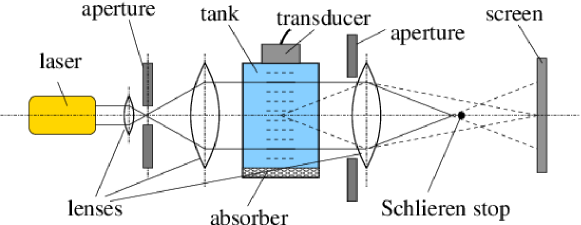
The data are collected with a Schlieren optical system where in the experiment an acoustic pressure is emitted into a water tank (see Figure 9). The Schlieren optical system outputs the intensity pattern of light passing through the tank which is proportional to the square of the line integral of the pressure along the light path.

For practical aspects on the realization of Schlieren systems and more background information on such measurement devices we refer to [4, 6, 10, 13, 20, 21, 26].

Figure 9: Schlieren optical system. The pressure field in the tank is reconstructed from Schlieren data acquired at different angles $\sigma_{i}$, $i\in\{0,\dots,N-1\}$ of rotation of the schlieren system.

4.1 Mathematical modelling

Let $H$ and $D:=\{\boldsymbol{\xi}\in\mathbb{R}^{2}\,:|\boldsymbol{\xi}|<1\}$ denote the height and an arbitrary cross-section of the tank, respectively. The pressure (to be reconstructed) within the tank is represented by a function $p:D\times[0,H]\to\mathbb{R}$. At each recording angle $\boldsymbol{\sigma}_{i}\in S^{1}$, $i=0,\dots,N-1$ the Schlieren system outputs

$$P_{i}(s,z):=\left(\int_{\mathbb{R}}p(s\boldsymbol{\sigma}_{i}+r\boldsymbol{\sigma}_{i}^{\bot},z)\,dr\right)^{2}\;,\quad z\in[0,H]\,,\ s\in I\,,$$

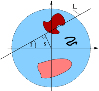
where $I:=[-1,1]$ and the parameter $s$ corresponds to the signed distance of the line $L_{i}(s):=s\boldsymbol{\sigma}_{i}+\mathbb{R}\boldsymbol{\sigma}_{i}^{\bot}$ from the origin in $D$, see Figure 10. In the following the height parameter $z$ is fixed. We aim to reconstruct the pressure function $x:D\to\mathbb{R}$ defined by $x(\boldsymbol{\xi}):=p(\boldsymbol{\xi},z)$ from data $F_{i}(x)(s):=P_{i}(s,z)$.

Figure 10: Cross section of the tank. The Schlieren system outputs squares of integrals over the lines $L_{i}(s)$, with unit normal $\boldsymbol{\sigma}_{i}=(\cos\varphi,\sin\varphi)$ and signed distance $s$ from the origin.

Now Schlieren tomography can be formulated as the problem of solving the system of operator equations

$$F_{i}(x)=y^{\delta,i}\,,\quad i=0,\dots,N-1\,,$$

for given noisy data $y^{\delta,i}$.

4.2 Abstract formulation in Hilbert–space

Let

$$\mathrm{R}_{i}:C_{0}^{\infty}(D)\to C_{0}^{\infty}(I):\quad x\mapsto\mathrm{R}_{i}(x):=\left(s\mapsto\int_{\mathbb{R}}x(s\boldsymbol{\sigma}_{i}+r\boldsymbol{\sigma}_{i}^{\bot})\,dr\right)$$

denotes the Radon transform, and $F_{i}=\mathrm{R}_{i}^{2}$ denotes the Schlieren transform.

Theorem 2.

The operators $\mathrm{F}_{i}$, $i\in\{0,\dots,N-1\}$ can be continuously extended on $H_{0}^{1}(D)$:

$$\mathrm{F}_{i}:H_{0}^{1}(D)\to L^{2}(I)\;.$$

Moreover, $\mathrm{F}_{i}$ is Fréchet differentiable and the Fréchet derivative of $\mathrm{F}_{i}$ at $x$ is given by

$$\mathrm{F}_{i}^{\prime}[x](h) =2\mathrm{R}_{i}(x)\mathrm{R}_{i}(h)\,.$$ (21)

Proof.

Let $x\in C_{0}^{\infty}(D)$. By applying the Cauchy Schwarz inequality two times,

$$\|\mathrm{F}_{i}(x)\|^{2}_{L^{2}} =\int_{-1}^{1}\left[\left(\int_{\mathbb{R}}x(s\boldsymbol{\sigma}_{i}+r\boldsymbol{\sigma}_{i}^{\bot})\chi_{D}(s\boldsymbol{\sigma}_{i}+r\boldsymbol{\sigma}_{i}^{\bot})\,dr\right)^{2}\right]^{2}ds$$ (22)

$$\leq\int_{-1}^{1}\left(2\int_{\mathbb{R}}x(s\boldsymbol{\sigma}_{i}+r\boldsymbol{\sigma}_{i}^{\bot})^{2}\chi_{D}(s\boldsymbol{\sigma}_{i}+r\boldsymbol{\sigma}_{i}^{\bot})\,dr\right)^{2}ds$$

$$\leq 8\int_{-1}^{1}\left(\int_{\mathbb{R}}x(s\boldsymbol{\sigma}_{i}+r\boldsymbol{\sigma}_{i}^{\bot})^{4}\,dr\right)ds=8\|x\|^{4}_{L^{4}}\,.$$

Using Sobolev’s embedding theorem (see [1]), it follows that

$$\|\mathrm{F}_{i}(x)\|^{2}_{L^{2}}\leq 8\cdot\|x\|_{L^{4}}^{4}\leq C\,\|x\|_{H^{1}}^{4}$$ (23)

for some positive constant $C$. Therefore, $\mathrm{F}_{i}$ extends, by continuity, to an operator $H_{0}^{1}(D)\to L^{2}(D)$.

Now let $\mathrm{F}_{i}^{\prime}[x]$ be defined by (21). Obviously $\mathrm{F}_{i}^{\prime}[x]$ is a bounded linear operator. Moreover, from the Cauchy Schwarz inequality it follows that

$$\|\mathrm{F}_{i}(x+h)-\mathrm{F}_{i}(x)-\mathrm{F}_{i}^{\prime}[x](h)\|_{L^{2}}^{2} =\|\mathrm{R}_{i}^{2}(x+h)-\mathrm{R}_{i}^{2}(x)-2\mathrm{R}_{i}(x)\mathrm{R}_{i}(h)\|_{L^{2}}^{2}$$

$$=\|R^{2}_{i}(h)\|_{L^{2}}^{2}=\|\mathrm{F}_{i}(h)\|_{L^{2}}^{2}\leq C\|h\|_{H^{1}}^{4}\,.$$

Therefore, we have

$$\lim_{h\to 0}\|\mathrm{F}_{i}(x+h)-\mathrm{F}_{i}(x)-\mathrm{F}_{i}^{\prime}[x](h)\|_{L^{2}}/\|h\|_{H^{1}}=0\,,$$

which implies that $\mathrm{F}_{i}^{\prime}[x]$ is the Fréchet derivative of $\mathrm{F}_{i}$ at $x$. ∎

We denote by $\mathrm{R}_{i}^{\sharp}$ the adjoint of $\mathrm{R}_{i}$, considered as an operator from $L^{2}(D)$ into $L^{2}(I)$ [17], which is given by

$$\mathrm{R}_{i}^{\sharp}:L^{2}(I)\to L^{2}(D)\quad y\mapsto\bigg{(}\boldsymbol{\xi}\mapsto\mathrm{R}_{i}^{\sharp}(y)(\boldsymbol{\xi}):=y(\langle\boldsymbol{\xi},\boldsymbol{\sigma}_{i}\rangle)\bigg{)}\,.$$ (24)

With this operator we can define the adjoint of $F_{i}^{\prime}[x]$:

Theorem 3.

The adjoint $\mathrm{F}_{i}^{\prime}[x]^{\ast}:L^{2}(I)\to H_{0}^{1}(D)$ of $\mathrm{F}_{i}^{\prime}[x]$ is given by $y\mapsto\mathrm{F}_{i}^{\prime}[x]^{\ast}(y)=:q$, where $q$ is the unique solution of

$$\left(\mathrm{I}-\Delta\right)q=2\mathrm{R}_{i}^{\sharp}(\mathrm{R}_{i}(x)y)$$ (25)

in $H_{0}^{1}(D)$. Here $\Delta$ denotes the Laplace operator on $H_{0}^{1}(D)$.

Proof.

Let $x\in H^{1}_{0}(D)$. We remark that $\mathrm{F}_{i}^{\prime}[x]^{\ast}$ is defined by

$$\langle\mathrm{F}_{i}^{\prime}[x](h),y\rangle_{L^{2}}=\langle h,\mathrm{F}_{i}^{\prime}[x]^{\ast}(y)\rangle_{H^{1}}$$ (26)

for all $y\in L^{2}(D)$ and $x\in H^{1}_{0}(D)$.

1. Using Fubini’s theorem and (24), the left hand side of (26) can be rewritten as follows

   $$\langle\mathrm{F}_{i}^{\prime}[x](h),y\rangle_{L^{2}} =2\int_{-1}^{1}\left(y(s)\mathrm{R}_{i}(x)(s)\int_{\mathbb{R}}h(s\boldsymbol{\sigma}_{i}+r\boldsymbol{\sigma}_{i}^{\bot})\,dr\right)ds$$ (27)

   $$=2\int_{B}h(\boldsymbol{\xi})y(\langle\boldsymbol{\xi},\boldsymbol{\sigma}\rangle)\mathrm{R}_{i}(x)(\langle\boldsymbol{\xi},\boldsymbol{\sigma}\rangle)\mathrm{d}\boldsymbol{\xi}$$

   $$=\langle h,2\mathrm{R}_{i}^{\sharp}(\mathrm{R}_{i}(x)y)\rangle_{L^{2}}\,.$$

2. The left hand side of (26) reads as follows

   $$\langle h,\mathrm{F}_{i}^{\prime}[x]^{\ast}(y)\rangle_{H^{1}} =\langle h,\mathrm{F}_{i}^{\prime}[x]^{\ast}(y)\rangle_{L^{2}}+\langle\nabla h,\nabla\mathrm{F}_{i}^{\prime}[x]^{\ast}(y)\rangle_{L^{2}}$$ (28)

   $$=\langle h,\mathrm{F}_{i}^{\prime}[x]^{\ast}(y)-\Delta\mathrm{F}_{i}^{\prime}[x]^{\ast}(y)\rangle_{L^{2}}$$

   $$=\langle h,(1-\Delta)\mathrm{F}_{i}^{\prime}[x]^{\ast}(y)\rangle_{L^{2}}$$

   since $h$ vanishes at the boundary of $D$.

Inserting (27) and (28) in (26) concludes the proof. ∎

4.3 Numerical reconstruction

According to (25) the lLK method for Schlieren tomography reads as follows

$$x_{n+1}=x_{n}-2\mu^{2}\omega_{n}(\mathrm{I}-\Delta)^{-1}R^{\sharp}_{[n]}\bigg{(}\mathrm{R}_{[n]}(x_{n})(\mathrm{F}_{[n]}(x_{n})-y^{\delta,[n]})\bigg{)}\,,$$

and

$$\omega_{n}:=\omega_{n}(\delta^{[n]},y^{\delta})=\begin{cases}1&\|\mathrm{F}_{[n]}(x)-y^{\delta,[n]}\|>\tau\delta^{[n]},\\ 0&\mbox{ otherwise\,. }\end{cases}\,.$$ (29)

Here $2(\mathrm{I}-\Delta)^{-1}\mathrm{R}_{[n]}^{\sharp}(\mathrm{R}_{[n]}(x)y)$ denotes the unique solution of (25) with $y=(\mathrm{F}_{[n]}(x_{n})-y^{\delta,[n]})$ and $\mu$ is a scaling parameter that ensures $\|\mu\mathrm{F}_{i}^{\prime}[x]\|\leq 1$ in a closed ball around the starting value $x_{0}$.

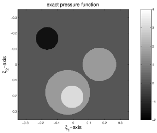
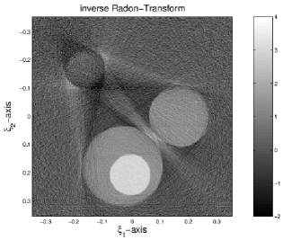
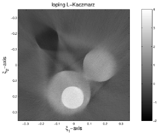
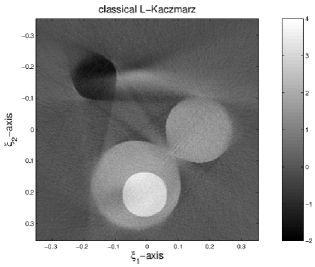
Figure 11: The pictures in the first line show the exact pressure function $x$ and the estimation with the Filter Back Projection (FBP) Algorithm from noisy data. The pictures in the second line show the results obtained with the lLK method and the LK method with $\tau=2.2$. All three simulations were performed with data with was perturbed by $0.01$ percent noise. Note that in our reconstruction negative values in $x$ can be detected, which cannot be detected by applying a FBP algorithm.

In the numerical implementation we approximated functions defined on $D$ and $I$ by piecewise linear splines. In the numerical experiment we used $\tau=2.2$ and $N=250$. The synthetic data set $y^{\delta,i}$, $i\in 0,\dots,N-1$, were generated by adding normal distributed random noise with $0.01\%$ noise level to the exact data. The phantom to be reconstructed is shown in Figure 11. It is a superposition of several characteristic functions. The reconstructions with the lLK method and the LK method were performed using the constant function $x_{0}(\boldsymbol{\xi})=0.01$ as initial guess.

Figure 12: The left image shows the decrease of the error using the lLK method and the LK method. The right picture shows the actually performed number of iterations within a cycle of the lLK method. Within the $9$–th cycle of the lLK method all $\omega_{n}=0$ and the iteration terminates.

We note that in all numerical experiments the lLK method applied to Schlieren tomography converged, even if the tangential cone condition was not satisfied.

4.4 Discussion

In contrast to the FPB algorithm the lLK method and the LK method are able to reconstruct both the positive and negative part of $u$. The lLK method reduces the artifact which is present in the reconstruction via the LK method.

The left image in Figure 12 shows that the number of actually computed Landweber steps per cycle in the lLK method is rapidly decreasing. Moreover, the norm of the error in the reconstruction with the lLK method is below the error of the LK method. Actually, the regularized solution $x_{n_{\ast}^{\delta}}$ of the lLK method is a better approximation of the true solution than all iterates of the LK method.

Since the used measuring data are squared numbers, there are two solutions, one with a positive sign and one with a negative sign. Our numerical simulations showed that a strictly positive initial guess $x_{0}$ leads to a numerical reconstruction $x_{n_{\ast}^{\delta}}$ with positive mean value.

5 Conclusion

We applied the abstract theory of the first part of this article to thermoacoustic computed tomography, to an inverse problem for semiconductors and to Schlieren tomography. In all applications the lLK method turned out to be an efficient iterative regularization method.

E-mail address: markus.haltmeier@uibk.ac.at
E-mail address: richard.kowar@uibk.ac.at
E-mail address: a.leitao@ufsc.br
E-mail address: otmar.scherzer@uibk.ac.at

References

• [1] R.A. Adams, Sobolev spaces, Academic Press, New York, 1975.
• [2] V.A. Andreev, A.A. Karabutov, S. V. Solomatin, E. V. Savateeva, V. Aleynikov, Y. V. Zhulina, R. D. Fleming, and A. A. Oraevsky, Opto–acoustic tomography of breast cancer with arc–array transducer, Biomedical Optoacoustics (San Jose, CA, USA), vol. 3916, 2000, pp. 36 – 47.
• [3] L. Borcera, Electrical impedance tomography, Inverse Problems 18 (2002), no. 6, R99–R136.
• [4] M. A. Breazeale, Schlieren photography in Physics, Proc. SPIE 3581 (1998), 41–47.
• [5] P. Burgholzer, C. Hofer, G. Paltauf, M. Haltmeier, and O. Scherzer, Thermoacoustic tomography with integrating area and line detectors, IEEE Trans. Ultrason. Ferroelec. Freq. Contr. 52 (2005), 1577 – 1583.
• [6] T. Charlebois and R. Pelton, Quantitative 2d and 3d Schlieren imaging for acoustic power and intensity measurements, Medical Electronics (1995), 789–792.
• [7] H.W. Engl, M. Hanke, and A. Neubauer, Regularization of inverse problems, Kluwer Academic Publishers, Dordrecht, 1996.
• [8] M. Haltmeier, A. Leitão, and O. Scherzer, Regularization of systems of nonlinear ill-posed equations: I. convergence analysis, submitted (2006).
• [9] M. Haltmeier, O. Scherzer, P. Burgholzer, R. Nuster, and G. Paltauf, Thermoacoustic tomography & the circular radon transform: Exact inversion formula, submitted (2006).
• [10] A. Hanafy and C. I. Zanelli, Quantitative real-time pulsed Schlieren imaging of ultrasonic waves, Proc. IEEE Ultrasonics Symposium 2 (1991), 1223–11227.
• [11] R. Kowar and O. Scherzer, Convergence analysis of a Landweber-Kaczmarz method for solving nonlinear ill-posed problems, Ill posed and inverse problems (book series) 23 (2002), 69–90.
• [12] R.A Kruger, W.L. Kiser, D.R. Reinecke, G.A. Kruger, and K.D. Miller, Thermoacoustic molecular imaging of small animals, Molecular Imaging 2 (2003), no. 2, 113–123.
• [13] E. G. LeDet and C. I. Zanelli, A novel, rapid method to measure the effective aperture of array elements, IEEE Ultrasonics Symposium (1999), –.
• [14] A. Leitao, P.A. Markowich, and J.P. Zubelli, Inverse problems for semiconductors: Models and methods, ch. in Transport Phenomena and Kinetic Theory: Applications to Gases, Semiconductors, Photons, and Biological Systems, Ed. C. Cercignani and E. Gabetta, Birkhäuser, Boston, 2006.
• [15]  , On inverse dopping profile problems for the stationary voltage-current map, Inv.Probl. 22 (2006), 1071–1088.
• [16] A.K. Louis and E.T. Quinto, Local tomographic methods in sonar, Surveys on solution methods for inverse problems, Springer, Vienna, 2000, pp. 147–154.
• [17] F. Natterer, The mathematics of computerized tomography, SIAM, Philadelphia, 2001.
• [18] Frank Natterer, Algorithms in tomography, State of the Art in Numerical Analysis, vol. 63, 1997, pp. 503–524.
• [19] G. Paltauf, R. Nuster, M. Haltmeier, and P. Burgholzer, Photoacoustic tomography using a mach–zehnder interferometer as acoustic line detector, Applied Optics (2006), accepted.
• [20] T. A. Pitts, J. F. Greenleaf, Jian-yu Lu, and R. R. Kinnick, Tomographic Schlieren imaging for measurment of beam pressure and intensity, Proc. IEEE Ultrasonics Symposium (1994), 1665–1668.
• [21] C.V. Raman and N. S. Nath, The diffraction of light by high frequency ultrasonic waves: Part 1, Proc. Indian Acad. Sci 2 (1935), 406–412.
• [22] X.D. Wang, G. Pang, Y.J. Ku, X.Y. Xie, G. Stoica, and L.V. Wang, Noninvasive laser-induced photoacoustic tomography for structural and functional in vivo imaging of the brain, Nature Biotechnology 21 (2003), 803–806.
• [23] M. Xu and L.V. Wang, Analytic explanation of spatial resolution related to bandwidth and detector aperture size in thermoacoustic or photoacoustic reconstruction, Physical Review E 67 (2003), 1–15.
• [24]  , Photoacoustic imaging in biomedicine, Review of Scientific Instruments 77 (2006), no. 4, 041101.
• [25] Y. Xu, L.V. Wang, G. Ambartsoumian, and Kuchment P., Reconstructions in limited-view thermoacoustic tomography, Medical Physics 31 (2004), no. 4, 724–733.
• [26] C. I. Zanelli and M. M. Kadri, Measurements of acoustic pressure in the non-linear range in water using quantitative Schlieren, Proc. IEEE Ultrasonics Symposium 3 (1994), 1765–1768.