MixMix: All You Need for Data-Free Compression Are Feature and Data Mixing
Abstract
User data confidentiality protection is becoming a rising challenge in the present deep learning research. Without access to data, conventional data-driven model compression faces a higher risk of performance degradation. Recently, some works propose to generate images from a specific pretrained model to serve as training data. However, the inversion process only utilizes biased feature statistics stored in one model and is from low-dimension to high-dimension. As a consequence, it inevitably encounters the difficulties of generalizability and inexact inversion, which leads to unsatisfactory performance. To address these problems, we propose MixMix based on two simple yet effective techniques: (1) Feature Mixing: utilizes various models to construct a universal feature space for generalized inversion; (2) Data Mixing: mixes the synthesized images and labels to generate exact label information. We prove the effectiveness of MixMix from both theoretical and empirical perspectives. Extensive experiments show that MixMix outperforms existing methods on the mainstream compression tasks, including quantization, knowledge distillation and pruning. Specifically, MixMix achieves up to 4% and 20% accuracy uplift on quantization and pruning, respectively, compared to existing data-free compression work.
1 Introduction
To enable powerful deep learning models on the embedded and mobile devices without sacrificing task performance, various model compression techniques have been discovered. For example, neural network quantization [gong2019dsq, hubara2017qnn, li2019apot, zhu2016ttq] converts 32-bit floating-point models into low-bit fixed point models and benefits from the acceleration of fixed-point computation and less memory consumption. Network pruning [dong2017obslayer, han2015deepcompress, theis2018fisherprune] focuses on reducing the redundant neural connections and finds a sparse network. Knowledge Distillation (KD) [hinton2015distilling, polino2018distillation] transfers the knowledge in the large teacher network to small student networks.


However, one cannot compress the neural networks aggressively without the help of data. As an example, most full precision models can be safely quantized to 8-bit by directly rounding the parameters to their nearest integers [krishnamoorthi2018quantizing, nagel2019dfq]. However, when the bit-width goes down to 4, we have to perform quantization-aware training using the data collected from users to compensate for the accuracy loss. Unfortunately, due to the increasing privacy protection issue111https://ec.europa.eu/info/law/law-topic/data-protection_en, one cannot get user data easily. Moreover, the whole ImageNet dataset contains 1.2M images (more than 100 gigabytes), which consumes much more memory space than the model itself. Therefore, the data-free model quantization is more demanding now.
Recently, many works [cai2020zeroq, haroush2020knowledge, yin2020deepinverse] propose to invert images from a specific pretrained model. They try to match the activations’ distribution by comparing the recorded running mean and running variance in the Batch Normalization (BN) [ioffe2015bn] layer. Data-free model compression with the generative adversarial network is also investigated in [chen2019dafl, DBLP:journals/corr/abs-1912-11006, dfqgan]. All these works put their focus on developing a better criterion for inverting the data from a specific model. We call this type of data as model-specific data.
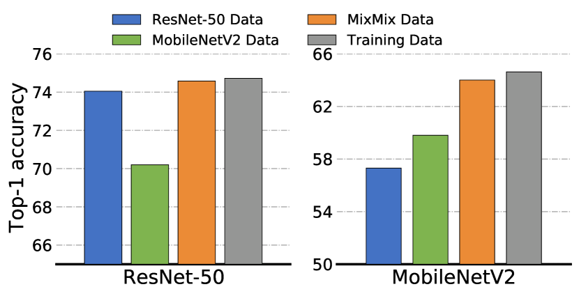
We identify two problems of model-specific data. First, the synthesized images generated by a specific model are biased and cannot be generalized to another. For example, in DeepInversion [yin2020deepinverse], synthesizing 215k 224224 resolution images from ResNet-50v1.5 [res50v1.5] requires 28000 GPU hours. These images cannot be used for another model easily. As we envisioned in Fig. 1, data inverted from MobileNetV2 has 4% higher accuracy than ResNet-50 data on MobileNetV2 quantization and vice versa. Therefore, model-specific data inversion requires additional thousands of GPU hours to adapt to compression on another model. Second, due to the non-invertibility of the pretrained model, model-specific data results in inexact synthesis. A simple example is not hard to find: given a ReLU layer that has 0 in its output tensor, we cannot predict the corresponding input tensor since the ReLU layer outputs 0 for all negative input. As a result, finding the exact inverse mapping of a neural network remains a challenging task.
In this work, we propose MixMix data synthesis algorithm that can generalize across different models and applications, which contributes to an overall improvement for data-free compression. MixMix contains two sub-algorithms, the first one is Feature Mixing which utilizes the universal feature produced by a collection of pre-trained models. We show that Feature Mixing is equal to optimize the maximum mean discrepancy between the real and synthesized images. Therefore, the optimized data shares high fidelity and generalizability. The second algorithm is called Data Mixing that can narrow the inversion solution space to synthesize images with exact label information. To this end, we summarize our core contributions as:
-
1.
Generalizability: We propose Feature Mixing that can absorb the knowledge from widespread pre-trained architectures. As a consequence, the synthesized data can generalize well to any models and applications.
-
2.
Exact Inversion: We propose Data Mixing which is able to prevent incorrect inversion solutions. Data Mixing can preserve correct label information.
-
3.
Effectiveness: We verify our algorithm from both theoretical and empirical perspectives. Extensive data-free compression applications, such as quantization, pruning and knowledge distillation are studied to demonstrate the effectiveness of MixMix data, achieving up to 20% absolute accuracy boost.
2 Related Works
Data-Driven Model Compression
Data is an essential requirement in model compression. For example, automated exploring compact neural architectures [zoph2016nas, liu2018darts] requires data to continuously train and evaluate sub-networks. Besides the neural architecture search, quantization is also a prevalent method to compress the full precision networks. For the 8-bit case where the weight quantization nearly does not affect accuracy, only a small subset of calibration images is needed to determine the activation range in each layer, which is called Post-training Quantization [banner2019aciq, krishnamoorthi2018quantizing]. AdaRound [nagel2020adaround] learns the rounding mechanism of weights and improves post-training quantization by reconstructing each layer outputs. Quantization-aware finetuning [Esser2020LEARNED] can achieve near-to-original accuracy even when weights and activations are quantized to INT4. But this method requires a full training dataset as we mentioned. Apart from quantization, network pruning and knowledge distillation are also widely explored [hinton2015distilling, he2017channel].
Data-Free Model Compression
The core ingredient in data-free model compression is image synthesis so that no real images are needed. Currently, the generation process can be classified into two categories, (1) directly learn images by gradient descent or (2) train a generative adversarial network (GAN) to produce images. DAFL [chen2019dafl] and GDFQ [choi2020data] apply GAN to generate images and learn the student network. This type of work achieves good results on tiny dataset. However, training large-scale GAN requires significant efforts. A parallel ax in image synthesis is model inversion [mahendran2015understanding, mahendran2016visualizing]. Mordvintsev et al. proposed DeepDream [mordvintsev2015inceptionism] to ‘dream’ objects features onto images from a single pre-trained model. Recently, DeepInversion [yin2020deepinverse] uses the BN statistics variable as an optimization metric to distill the data and obtain high-fidelity images. BN scheme has also achieved improvements in other tasks: ZeroQ [cai2020zeroq] and the Knowledge Within [haroush2020knowledge] use distilled dataset to perform data-free quantization, but their methods are model-specific, i.e., one generated dataset can only be used for one model’s quantization. Our MixMix algorithm mainly focus on the direct optimization of data, however, it is also applicable to generative data-free application.
3 Preliminary
In this section, we will briefly discuss the background of how to synthesize images from a single pretrained model, then we will discuss two challenges of this method.
3.1 Model-Specific Data Inversion
Suppose we have a trainable image with the size of (in ImageNet dataset [deng2009imagenet], the size is ) and a pretrained network , the Inceptionism [mordvintsev2015inceptionism] can invert the knowledge by assigning the image with a random label , since the networks have already captured the class information. Using the cross-entropy loss, the image can be optimized by
| (1) |
Recently, [cai2020zeroq, haroush2020knowledge, yin2020deepinverse] observe that the pretrained networks have stored the activation statistics in the BN layers (i.e. running mean and running variance). Consequently, it is reasonable for synthesized images to mimic the activation distribution of the natural images in the network. Therefore, assuming the activation (regardless of the batch) in each layer is Gaussian distributed, the BN statistics loss can be defined as
| (2) |
where () is the mean (variance) of the synthesized images activation in -th layer while () is the stored running mean (variance) in the BN layer. Note that we can replace the MSE loss to Kullback-Leibler divergence loss as did in [haroush2020knowledge].
In addition, an image prior loss can be imposed on to ensure the images are generally smooth. In [haroush2020knowledge], the prior loss is defined as the MSE between and its Gaussian blurred version . In this work, we use the prior loss defined in [yin2020deepinverse]: , which is the sum of variance and norm regularization. Combining these three losses, the final minimization objective of knowledge inversion for a specific model can be formulated as:
| (3) |
3.2 Biased Feature Statistics
Model ImageNet Res50 Data MobV2 Data ResNet-50 0.018 0.049 0.144 MobileNetV2 0.722 4.927 1.498
For image synthesis tasks, the real ImageNet dataset could be viewed as the global minimum, which can be utilized to perform model compression on any neural architectures. However, we find that the data synthesized from one model cannot be directly applied to another different architecture. Example results demonstrated in Fig. 1 show that data synthesized on ResNet-50 gets bad quantization results on MobileNetV2 (4% lower) and vice versa.
We conjecture the reason for this phenomenon is the different feature statistics learned in different CNNs. In each neural network, the distribution characteristics of the training data are encoded and processed in its unique feature space (i.e. unique BN statistics). Therefore, extract the feature information from this neural network leads to biased statistics. To test this, we train images from ResNet-50 and MobileNetV2 by Eq. (3) and validate the synthesized images on these architectures. Results in Table 1 show that of the MobileNetV2 data is high when evaluated on ResNet50. Interestingly, in an opposite way, ResNet-50 data also has poor performance on MobileNetV2. However, as shown in Table 1, always remains in low-level regardless of model in the case of real ImageNet data.
3.3 Inexact Inversion
Apart from BN statistics loss , the cross-entropy loss desires to learn an inverted mapping from label to input images, denoted by . According to [behrmann2019invertible], a residual block is invertible if it has less than 1 Lipschitz constant and the same input-output dimension (i.e. ). We find the latter one is not true for all classification models, since the label dimension is and input dimension is for the ImageNet classification task. This dimension difference can produce a huge solution space for image inversion. Let us consider an example of the average pooling layers:
Example 3.1.
Consider a AvgPool layer , where and are the input and weight vectors. This AvgPool layers is non-invertible because given output , any inputs that has same mean as will suffice the condition.
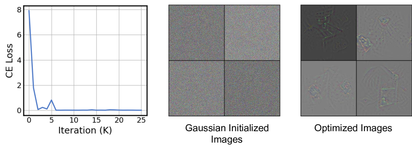
Therefore, finding the exact input is infeasible in such a large space. In fact, almost every CNN has a AvgPool layer before the final fully-connected layer. To visualize this, we optimize 4 images using and and plot the training curve in Fig. 3. It is clear that CE loss is easy to optimize, yet we cannot invert real images that contain rich class information.

4 Methodology
In this section, we introduce the proposed MixMix algorithm, which can improve both the generalizability and the invertibility of the dataset.
4.1 Feature Mixing
Before delving into the proposed algorithm, we would like to discuss the general problem of comparing samples from two probability distributions. This problem is of great interest in many areas such as bioinformatics where two image types are evaluated to determine if they come from the same tissues. In the case of image synthesis, we also need to evaluate if the generated images preserve high fidelity. Formally, given two distributions and with their random variables defined on a topological space and observations () that are independently and identically distributed (i.i.d.) from and , can we find some methods to determine if ? In [dudley2018real, Lemma 9.3.2], this problem is well-defined as
Lemma 4.1 ([dudley2018real]).
Let be a metric space, and let be two Borel probability measures defined on . Then if and only if for all , where is the space of bounded continuous functions on .
However, evaluating all in the finite settings is not practical. Fortunately, Gretton et al. [gretton2012kernel] proposed the maximum mean discrepancy that can be represented by:
| (4) |
where is a class of function which is much smaller than . We will directly give two results that are related to MMD theory and the BN statistics loss. The detailed derivation is located in the appendix.
-
1.
Let be a reproducing kernel Hilbert space (RKHS), and when we set to , the squared MMD is given by.
(5) where is called the mean embedding of . we can use the feature extractor of the CNNs and its feature-map to define a reproducing kernel. Therefore the running mean and variance222The variance can be defined in the kernel’s second-order space. in BN layers can be treat to the mean embedding of . Thus optimizing the is equivalent to minimize the between the real images and the synthesized images.
-
2.
[gretton2012kernel, Theorem 5] states that the kernel for feature extraction must be universal333The universal means that, for any given and there exists a such that the max norm . so that we have if and only if .
These two results indicate that if the neural network is universal and the of synthesized images is 0, we could say the generated images are very close to real images. But it turns out few neural networks are universal and are only possible for extremely deep or wide ones [lin2017does, lu2017expressive]. In Sec. 3.2, we show that different CNN has different feature statistics. And the data generated from one model is hard to be transferred to another one. This empirical evidence further illustrates the lack of universality in one model. We hereby propose Feature Mixing, which gathers the knowledge in the model zoo and aims to average out the feature bias produced by each individual. We expect the aggregation of pre-trained models can improve the universality of their corresponding RKHS. To demonstrate that mixing features can improve the universality, we have the following theorem:
Theorem 4.2.
Assume there are neural networks with ReLU activation function (). Then, the averaged model is universal if , where is the averaged width.
Proof is available in the appendix. Although sufficing the ultimate universality may require a large , we anticipate increasing the number of features mixed can improve the quality as well as the generalizability of the generated data. To this end, we will show how to apply Feature Mixing during synthesis. Consider a pretrained model zoo , the Feature Mixing aims to optimize:
| (6) |
Note that we also add a prior loss on . However, assuming the identical size of each model , the training memory and computation is linearly scaled by the number of features we mix. Therefore, we add a hyper-parameter , which will decide how many models will be sampled from the model zoo for each batch of the data. The effect of will be studied in the experiments. Another problem is how to select model zoo, we expect different architecture families will contain different feature statistics, therefore we choose model families as many as possible in our model zoo.
4.2 Data Mixing
Another problem in image synthesis is that certain layers or blocks in neural network cause inexact inversion, as we described in Sec. 3.3. In this section, we show that we can mitigate this problem through Data Mixing. Denote two image-label pairs as and , we first randomly generate a binary mask . The elements in this mask will be set to 1 if it is located in the bounding box:
| (7) |
where are the left, right, down, up boundaries of the box. The center coordinate of the bounding box can be computed by . With this binary mask, we can mix the feature of data, given by
| (8) |
Here is a linear interpolation function that can resize the images to the same size of the bounding box. The mixed data now contains information from two images, thus we mix the label so that the CE loss becomes
| (9) |
where is computed as the ratio of bounding box area and the image area . Data Mixing is inspired by the success of mixing-based data-augmentations, such as CutMix [yun2019cutmix] and Mixup [zhang2017mixup]. They use mixed data and label to train a model that has stronger discriminative power. Indeed, such augmentation techniques is also helpful in our scope by generating the robust features that remain discriminative when being mixed. Moreover, in this work, data mixing is also used to reduce the inexact inversion solutions of the neural networks. Back to Example 3.1, for each iteration , we must suffice , where the input and output are mixed differently and therefore more restrictions are added when inverting the input. We also give an example to illustrate this:
Example 4.3.
Consider the same AvgPool layer in former discussion. If , then we have
| (10) |
Now assume a mixed input and output where the first two elements in come from another input image. Then we can obtain following relationships:
| (11) |
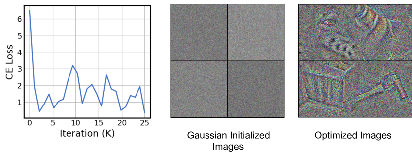
We can see that Data Mixing can help image inversion because the solution space in Eq. (11) is much smaller than Eq. (10). We also visualize the data-feature mixing using only CE and prior loss for image generation. The training curve as well as the optimized images are shown in Fig. 4. Notably, there are some basic shapes or textures in optimized images if we mix the data features.

Together with Feature Mixing, we formalize the MixMix data synthesis procedure in algorithm 1.
5 Experiments
We conduct our experiments on both CIFAR10 and ImageNet dataset. We set the subset size of Feature Mixing as except we mention it. We select 21 models in our pretrained model zoo, including ResNet, RegNet, MobileNetV2, MobileNetV3, MNasNet, VGG, SE-Net, DenseNet, ShuffleNetV2 [he2016resnet, radosavovic2020regnet, sandler2018mobilenetv2, howard2019searching, tan2019mnasnet, simonyan2014vgg, ma2018shufflenet, hu2018senet, huang2017densenet], etc. See detailed descriptions in appendix. The width and the height of the bounding box for data mixing are sampled from a uniform distribution. We use Adam [kingma2014adam] optimizer to optimize the images. Most hyper-parameters and implementation are aligned up with [yin2020deepinverse], such as multi-resolution training pipeline and image clip after the update. We optimize the images for 5k iteration and use a learning rate of 0.25 followed by a cosine decay schedule. To determine , we set it learnable and optimize it by gradient descent, details can be found in the appendix. Training 1024 MixMix images requires approximately 2 hours on 8 1080TIs.
5.1 Analysis of the Synthesized Images
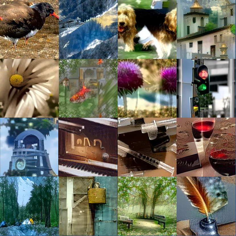
We present some qualitative evaluation in Fig. 5. Notably, MixMix data preserves high fidelity and resembles real images. To test the generalizability of the synthesized images, we report the average classification accuracy (as well as the standard deviation) on 21 different models in the model zoo. We also report the Inception Score (IS) [NIPS2016_8a3363ab] to evaluate the image quality.
Methods Size Average Acc. IS DeepDream-R50 [mordvintsev2015inceptionism] 224 24.98.23 6.2 DeepInversion-R50 [yin2020deepinverse] 224 85.965.80 60.6 BigGAN [brock2018bigGAN] 256 N/A 178.0 SAGAN [zhang2019SAGAN] 128 N/A 52.5 MixMix 224 96.951.53 92.9
It can be noted from Table 2 that model-specific data (from ResNet-50) has lower average accuracy. The proposed MixMix data achieves near 97% average accuracy and the stablest result. This means that our generated images have obvious class characteristics that all models can recognize. As a consequence, we can safely adopt it for all data-free applications and any architecture. We also compare with some GAN-based image synthesis methods where MixMix can achieve a comparable Inception Score.

5.2 Data-Free Quantization
In this section, we utilize the images generated by MixMix to conduct Post-Training Quantization (PTQ) and Quantization-Aware Training (QAT) on ImageNet. Here we adopt two state-of-the-art PTQ and QAT methods, namely BRECQ [li2021brecq] and LSQ [Esser2020LEARNED].
Post-Training Quantization
[li2021brecq] uses the block output reconstruction to optimize the rounding policy of weight quantization and the activation quantization range. We use 1024 images with a batch size of 32 to optimize the quantized model. Each block is optimized by 20k iterations. We compare ZeroQ [cai2020zeroq] and The Knowledge Within [haroush2020knowledge] (abbreviated as KW in the this paper) data on ResNet-50, MobileNet-b (modified version of MobileNetV1 [howard2017mobilenets] without BN and ReLU after the depthwise convolutional layers), MobileNetV2, and MNasNet. To fairly compare results, we implement ZeroQ and KW to the same pre-trained models and apply the same quantization algorithm. Results are demonstrated in Table LABEL:tab_ptq. For ResNet-50 4-bit quantization, MixMix data has comparable results with the real images (only 0.14% accuracy drop). When the bit-width of weight goes down to 2, the quantization becomes more aggressive and requires high-fidelity data for calibration. In that case, MixMix still achieves the lowest degradation among the existing methods. We next verify data-free quantization on three mobile-platform networks, which face a higher risk of performance degeneration in compression. It can be seen that 4-bit quantization on lightweight networks generally will have much higher accuracy loss even using real images. However, MixMix data still reaches close-to-origin results. As an example, ZeroQ and KW only reach 49.83% and 59.81% accuracy on MobileNetV2, respectively. Whereas, MixMix can boost the performance to 64.01%.