Dynamically Consistent Approximate Rational Solutions to the Thomas-Fermi Equation

Abstract.

We construct two rational approximate solutions to the Thomas-Fermi (TF) nonlinear differential equation. These expressions follow from an application of the principle of dynamic consistency. In addition to examining differences in the predicted numerical values of the two approximate solutions, we compare these values with an accurate numerical solution obtained using a fourth-order Runge-Kutta method. We also present several new integral relations satisfied by the bounded solutions of the TF equation

1. Introduction

The major purpose of this paper is to construct a new rational approximation to the Thomas-Fermi equation

(1.1) $$\frac{d^{2}y\left(x\right)}{dx^{2}}=\frac{y\left(x\right)^{\frac{3}{2}}}{x^{\frac{1}{2}}},$$

with boundary conditions

(1.2) $$y\left(0\right)=1,y\left(\infty\right)=0.$$

This equation arises in the modeling of certain phenomena in the atomic structure of matter ([1], [2]).

Since it is expected that no exact analytical solution formula exists for the general solution in terms of a finite combination of elementary functions, a broad range of approximate solutions have been derived ([3], [4], [5], [6], [7], [8]). The mathematical procedures used to obtain these expressions include variational methods ([3], [6]), the use of iteration techniques [4], application of the Adomian decomposition method [5], homotopy analysis [7], and rational approximations [8]. The indicated references ([3], [4], [5], [6], [7], [8]) are but a small subset of the hundreds of publications on this subject. Note that the existence of such a substantial research literature is due, in large part, to the fact that this thorny boundary-value problem has drawn out a significant number of ideas as to how approximations to its solutions should be done.

The purpose of this paper is to use a new methodology to construct approximate solutions to the Thomas-Fermi (TF) equation. We do this within the framework of the concept or principle of dynamic consistency [9] and the restrictions that it imposes on any mathematical representation of the forms used for rational approximations to a TF equation solution. We demonstrate that this is rather easy to do.

In outline, Section 2 provides a summary of several of the general, exact, and for the most part qualitative properties of the TF equation [10]. This section includes several new results of the authors. Section 3 introduces and defines the concept of dynamic consistency [9] and it is used in Section 4 to construct two elementary rational approximations to the TF solution. Finally, in the last section, we provide a summary of our results and discuss possible extensions to this work.

2. Preliminaries: Exact results

It turns out that even in the absence of knowledge of an explicit, exact solution for the TF equation many of the essential properties of such a solution can be derive. Below, we give a concise summary of these items and refer the reader to the paper of Hille [10] for proofs of some of these statements.

a) An exact solution to the TF equation is

(2.1) $$y\left(x\right)\equiv y_{s}\left(x\right)=\frac{144}{x^{3}}.$$

Note that it contains no arbitrary parameters and thus is not a special case of the (unknown) general solution. We denote it as, $y_{s}\left(x\right)$ and call it a singular or asymptotic solution in the sense that given a solution $y\left(x\right)$ then [10],

(2.2) $$\lim_{x\rightarrow\infty}(x^{3}y\left(x\right))=144.$$

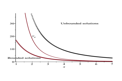
b) The curve $y\left(x\right)\equiv y_{s}\left(x\right)\$separates the bounded and unbounded solutions of the TF equation. This is evident from inspection of the flow-space as indicated in Figure 1.

Figure 1. Singular solution $y_{s}$ separating unbounded and bounded solutions

Note that since $y\left(x\right)\equiv 0$, is a solution, it follows that all solutions below the $y=y_{s}\left(x\right)$ curve are bounded and all solutions above are unbounded. The bounded solutions have a finite value for $y\left(0\right),$ while the unbounded have $y\left(0\right)=+\infty$.

c) The physical phenomena for which the TF equation was constructed requires

(2.3) $$y\left(x\right) >0,y^{\prime}\left(x\right)\equiv\frac{dy\left(x\right)}{dx}<0,0\leq x\,<\infty,$$

(2.4) $$y\left(0\right) =1,\ y\left(\infty\right)=0.$$

Observe that since $y^{\prime\prime}\left(x\right)>0,0<x<\infty,$ then all solutions are concave upward and this is consistent with the trajectory-flow given in Figure 1.

The figure also provides an overview of the bounded and unbounded trajectories of the TF equation.

d) For the bounded solutions

(2.5) $$0<y\left(x\right)<y\left(0\right)<\infty,y^{\prime}\left(0\right)<y^{\prime}\left(x\right)<0,y^{\prime\prime}\left(x\right)>0,0<x\,<\infty.$$

Further we have

(2.6) $$y^{\prime\prime}\left(x\right)=O\left(\frac{1}{\sqrt{x}}\right),x\rightarrow 0^{+}.$$

e) It is remarkable that $y^{\prime}\left(0\right)$ can be calculated to essentially any decimal place of accuracy [11]; defining the constant $B$ as follows,

(2.7) $$y^{\prime}\left(0\right)=-B,$$

we have [11]

(2.8) $$B=1.588071022611375\ldots.$$

f) For small $x$, $y\left(x\right)$ has the representation [4] for $y\left(0\right)=1$ and $y^{\prime}\left(0\right)=-B,$

$$y\left(x\right) =\left[1-Bx+\left(\frac{1}{3}\right)x^{3}-\left(\frac{2B}{15}\right)x^{4}+\cdots\right]$$

(2.9) $$\cdots+x^{3/2}\left[\frac{4}{3}-\left(\frac{2B}{5}\right)x+\left(\frac{3B^{2}}{70}\right)x^{2}\right.+\left.\left(\frac{2}{27}+\frac{B^{3}}{252}\right)x^{3}+\cdots\right].$$

g) The following “sum-rules”, involving integrals of $y\left(x\right),$have been derived by the authors. As far as we are aware, most of these are  new results pertaining to the solution (see Eqs. (1.1) and (1.2)) of the TF equation:

(2.10) $$\int_{0}^{\infty}\sqrt{x}y\left(x\right)^{3/2}dx=1,$$

(was derived in [15])

(2.11) $$\int_{0}^{\infty}y\left(x\right)dx=\frac{1}{2}\int_{0}^{\infty}x^{\frac{3}{2}}y\left(x\right)^{\frac{3}{2}}dx,$$

(2.12) $$B=\int_{0}^{\infty}\left[\left(\frac{dy}{dx}\right)^{2}+\frac{y^{\frac{5}{2}}}{\sqrt{x}}\right]dx$$

(2.13) $$B=\int_{0}^{\infty}\frac{y\left(x\right)^{3/2}}{\sqrt{x}}dx.$$

Let us derive the result in Eq. (2.12). Multiply both sides of the TF equation by $y\left(x\right):$

(2.14) $$yy^{\prime\prime}=\frac{y^{\frac{5}{2}}}{\sqrt{x}}.$$

Integrating once by parts and evaluating at $x=0$ and $x=\infty,$ gives

(2.15) $$y\left(\infty\right)y^{\prime}\left(\infty\right)-y\left(0\right)y^{\prime}\left(0\right)-\int_{0}^{\infty}\left(y^{\prime}\left(x\right)\right)^{2}dx=\int_{0}^{\infty}\frac{y^{\frac{5}{2}}}{\sqrt{x}}dx.$$

But $y\left(0\right)=1,y^{\prime}\left(0\right)=-B$ and $y\left(\infty\right)=y^{\prime}\left(\infty\right)=0;$ therefore, the result listed in Eq. (2.12) is obtained. The other relations can be derived using similar techniques.

Finally, we go back to Eq. (2.9) and demonstrate one possible way to derive it. First, observe that for small $x,$ the TF equation is approximated by the expression

(2.16) $$y^{\prime\prime}\left(x\right)\simeq\frac{1}{\sqrt{x}},$$

where $y\left(0\right)=1$ and $y^{\prime}\left(0\right)=-B.$ Integrating twice and imposing the just stated initial conditions gives

(2.17) $$y\left(x\right)\simeq 1-Bx+\left(\frac{4}{3}\right)x^{\frac{3}{2}},$$

corresponding to the first three terms of (2.9).

Let us now construct an iteration scheme to obtain a small$\ x$ representation for the TF equation. We assume it has the form

(2.18) $$y_{N+1}^{\prime\prime}(x) =\frac{\left[y_{N}\left(x\right)\right]^{\frac{3}{2}}}{\sqrt{x}},\ N=0,1,2,\ldots;$$

(2.19) $$y_{N}\left(0\right) =1,y_{N}^{\prime}\left(0\right)=-B,\$$

(2.20) $$y_{0}\left(x\right) =1.$$

Note that $y_{1}\left(x\right)$ is the result given in Eq. (2.17).

To calculate $y_{2}\left(x\right)$, we start with

$$y_{2}^{\prime\prime}(x) =\frac{\left[y_{1}\left(x\right)\right]^{\frac{3}{2}}}{\sqrt{x}}$$

(2.21) $$=\frac{\left[1-Bx+\left(\frac{4}{3}\right)x^{\frac{3}{2}}\right]^{\frac{3}{2}}}{\sqrt{x}}.$$

Expanding the expression in the brackets and retaining the first two terms gives

(2.22) $$\left[1-Bx+\left(\frac{4}{3}\right)x^{\frac{3}{2}}\right]^{\frac{3}{2}}=1-\left(\frac{3B}{2}\right)x+\cdots\ .$$

Thus it follows that

(2.23) $$y_{2}^{\prime\prime}\left(x\right)=\frac{1}{\sqrt{x}}-\left(\frac{3B}{2}\right)\sqrt{x}.$$

Integrating this equation twice, with the imposition of the initial conditions $y_{2}\left(0\right)=1,y_{2}^{{}^{\prime}}\left(0\right)=-B,$ gives

(2.24) $$y\left(x\right)=1-Bx+\left(\frac{4}{3}\right)x^{\frac{3}{2}}-\left(\frac{2B}{5}\right)x^{\frac{5}{2}}.$$

The result corresponds, respectively, to the first two terms in the brackets of Eq. (2.21).

Finally, with careful attention to which terms to retain, at each step of the iteration given by Eq. (2.18-2.20), the full result presented in Eq. (2.9) can be produced.

3. Dynamic consistency

Consider two systems $A$ and $B.$ Let system $A$ have the property $P.$ If system $B$ also has property $P,$ then $B$ is said to be dynamic consistent to $A$, with respect to property $P\$[9].

Dynamic consistency  (DC) has served as one of the fundamental principles of the nonstandard, finite difference methodology for constructing improved discrete models for the numerical integration of differential equations [9]. It serves as an assessment of the “closeness” or “fidelity” of two systems based on their mutually shared properties. Note that the systems $A$ and $B$ may not be of the same type object, structure or thing. For example, $A$ might be a physical system, while $B$ could be a mathematical model of $A.\$Likewise, $A$ might be a system of differential equations and $B$ a particular discretization of these equations. Thus DC is of general applicability and is available for use in diverse situations.

In the next section, we provide two ansatzes for approximate solutions to the TF equation, Our proposed solutions are to be DC with respect to the following properties of the exact, but unknown, solution to the second-order, nonlinear TF differential equation:

(3.1) $$\text{(i)}\ \ y\left(0\right)=1,y^{\prime}\left(0\right)=-B;$$

(3.2) $$\text{(ii)}\ \ 0<y\left(0\right)\leq 1,-B\leq y^{\prime}\left(x\right)<0,0\leq x<\infty;$$

(3.3) $$\text{(iii)}\ \ \lim_{x\rightarrow\infty}\left(x^{3}y\left(x\right)\right)=144\ ;\$$

(iv) the approximate solutions $y_{a}\left(x\right)$ are to be taken as rational functions of either $x$ or $\sqrt{x}$;

(v) the approximate solutions$,y_{a}\left(x\right)$, are to have one or the other of the following forms for small $x$;

(3.4) $$y_{a}\left(x\right)=\left\{\begin{array}[c]{c}1-Bx,\ \ \text{rational in }x;\\ 1-Bx+\left(\frac{4}{3}\right)x^{3/2},\text{ rational in }\sqrt{x}\end{array}\right.$$

4. Approximate solutions

We take the following two ansatzes to represent approximations to the solution of the TF equation

(4.1) $$y_{a}^{\left(1\right)}(x)=\frac{1}{1+Bx+\left(\frac{1}{144}\right)x^{3}},$$

(4.2) $$y_{a}^{\left(2\right)}\left(x\right) =\frac{1}{1+Bx-\left(\frac{4}{3}\right)x^{3/2}+Cx^{2}+\left(\frac{1}{144}\right)x^{3}},$$

(4.3) $$C =\frac{B^{2}}{2},$$

where $B=1.588071$, and as a consequence of (4.3), $C=1.260985.$

Close inspection of $\ y_{a}^{\left(1\right)}(x)$ and $y_{a}^{\left(2\right)}\left(x\right)$ shows that they are DC with the five conditions listed in section 3. Observe that $y_{a}^{\left(1\right)}\left(x\right)$ is a rational function of $x$, while $y_{a}^{\left(2\right)}\left(x\right)$ is a rational function of $\sqrt{x}.$

Figure 2. Plots of $y_{a}^{\left(1\right)}\left(x\right)$ $\left({}^{\_\_\_\_\_}\right)\$and $y_{a}^{\left(2\right)}\left(x\right)\ \left(\cdot\cdot\cdot\cdot\right)$

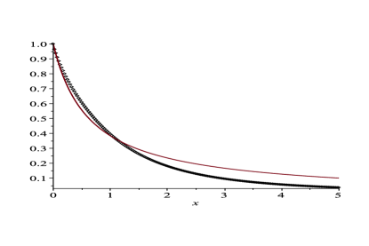
Figure LABEL:fig:2 gives plots of $y_{a}^{\left(1\right)}(x)$ and $y_{a}^{\left(2\right)}(x)$ vs. $x$. The two curves lie close to each other, but do not coincide, i.e.

(4.4) $$\left\{\begin{array}[c]{c}y_{a}^{\left(1\right)}(x)<y_{a}^{\left(2\right)}(x),\ 0<x<x_{0},\\ y_{a}^{\left(1\right)}(x)>y_{a}^{\left(2\right)}(x),\ \ x>x_{0}\end{array}\right.$$

with $x_{0}\approx 1.$

5. Discussion

In summary we have constructed two representations of approximate solutions to the TF equation. However, it must be stated that this equation is itself an approximation to an (unknown) equation describing atomic quantum phenomena ([1], [2]). In addition, all numerical procedures have errors associated with their algorithms and the hardware on which they are implemented.

The methodology used to generate the ansatzes, given in Eqs. (4.1) and (4.2, 4.3), is based on constructing for $y\left(x\right)$, the exact solution, rational functions such that the five conditions listed in section 3 are satisfied. An important benefit of this procedure is that the process is essentially algebraic and requires the introduction of no parameters which must be determined later in the construct. The $y_{a}^{\left(1\right)}(x)$ and $y_{a}^{\left(2\right)}(x)$ are constructed to be consistent with the $x-$small and $x-$large asymptotics. Thus, these representations possess great simplicity both in their manner of construction, as well as the lack of a need to introduce new parameters.

In Table 1 we compare the numerics of a fourth-order Runge-Kutta method and the values of $y\left(x\right)$ as calculated from our formulae for $y_{a}^{\left(1\right)}(x)$ and $y_{a}^{\left(2\right)}(x)$. Clearly, both analytic approximations and the numerical integration results are consistent, and in fact are in very good qualitative agreement with each other.

Table - 1 Numerical values of $y\left(x\right)$ and $y_{a}\left(x\right).$
$x$ $y\left(x\right)$ numerical [12] $y_{a}^{\left(1\right)}\left(x\right)$ $0.0$ $1.0000$ $1.0000$ $0.5$ $0.6070$ $0.5571$ $1.0$ $0.4240$ $0.3853$ $2.0$ $0.2430$ $0.2363$ $4.0$ $0.1840$ $0.1283$ $5.0$ $0.0789$ $0.1020$ $10.0$ $0.0243$ $0.0420$ $25.0$ $0.0035$ $0.0067$ $40.0$ $0.0011$ $0.0020$ $y_{a}^{\left(2\right)}\left(x\right)$ $1.0000$ $0.6102$ $0.3964$ $0.1817$ $0.0578$ $0.0378$ $0.0093$ $0.0013$ $0.0005$

Since the main task has been achieved, i.e., to demonstrate through explicit construction an alternative methodology for finding rational approximations for the solution of the TF equation, we now can proceed to the next stage, namely, determine a restriction or condition allowing us to access the overall validity or accuracy of our solutions. To do this, we consider the integral relations stated in Section 2. For our purposes, we select the sum-rule given in Eq. (2.12), mainly because it takes the form of an energy type integral [13], widely used throughout physics. In fact, inspection of Eq. (2.12) suggests the following correspondence

$$\left(\frac{dy}{dx}\right)^{2}\longrightarrow\text{ kinetic energy,}$$

$$\frac{y^{\frac{5}{2}}}{\sqrt{x}}\longrightarrow\ \text{potential energy.}$$

Note that the result in Eq. (2.12) can be used as a consistency check, since $B$ occurs in $y\left(x\right)$ which appears in the integral. Using $y_{a}^{\left(1\right)}(x)$ and $y_{a}^{\left(2\right)}(x)$ and carrying out the required numerical integration we find, respectively

$$B_{1}=1.584744,\ \ B_{2}=1.592931,$$

which are to be compared to the input value of

$$B=1.588071.$$

The fractional percentage errors are

$$E_{1}=\left(\frac{B-B_{1}}{B}\right)\cdot 100=0.21\%,\ E_{2}=\left(\frac{B-B_{2}}{B}\right)\cdot 100=-0.27\%.$$

Thus, with regard to the sum-rule, stated in Eq. (2.12), both rational approximations are essentially the same in their ability to satisfy the sum-rule.

Eventually, the next step in this research is to construct more complex rational approximations for the solution of the TF equation which incorporate further terms in the known asymptotic expansions for both $x-$small and $x-$large using Padé approximants [14].

References

- [1] E. Fermi, Rend. Acad. Naz. Lincei 6 (1927), 602-607
- [2] L. H. Thomas, Proc. Camb. Phil. Soc. 23 (1927), 452-548.
- [3] N. Anderson, A. M. Arthurs, and P. D. Roninson, Il Nuovo Cimento B Series 10, 57 (1968), 523-526.
- [4] G. I. Plindev and S. K. Pogrebnga, Journal of Physics B: Atomic and Molecular Physics 20, Number 17 (1987), L547.
- [5] G. Adomian, Applied Mathematics Letters 11, No. 3 (1998), 131-133.
- [6] M. Desaix, D. Anderson, and M. Lisak, European Journal of Physics 25, No. 6 (2004), 699-705.
- [7] (A. El-Nahhas, Acta Physica Polonica A 114, No. 4 (2008), 913-918.
- [8] W. Robin, Journal of Innovative Technology and Education 5, No. 1 (2018), 7-13.
- [9] R. E. Mickens, Journal of Difference equations and Applications 11, No.7 (2005), 645-653.
- [10] E. Hille, Proc. Nat. Acad Sci. USA 62, no. 1 (1969), 7-10.
- [11] F. M Fernández, Physics Letters A 365 (2007), 111
- [12] P. S. Lee and T.-Y. Wu, Chinese Journal of Physics 35, No. 6-11 (1997), 737-741.
- [13] J. R. Taylor, Classical Mechanics, University Science Books, Sausalito, CA, 2005.
- [14] M. A. Noor and S. T. Mohyud-Din, International Journal of Nonlinear Science 8, No. 1 (2009), 27-31
- [15] E. B. Baker, Physical Review 16 (1930), 630-647.