DCT-Mask: Discrete Cosine Transform Mask Representation for
Instance Segmentation

Abstract

Binary grid mask representation is broadly used in instance segmentation. A representative instantiation is Mask R-CNN which predicts masks on a $28\times 28$ binary grid. Generally, a low-resolution grid is not sufficient to capture the details, while a high-resolution grid dramatically increases the training complexity. In this paper, we propose a new mask representation by applying the discrete cosine transform(DCT) to encode the high-resolution binary grid mask into a compact vector. Our method, termed DCT-Mask, could be easily integrated into most pixel-based instance segmentation methods. Without any bells and whistles, DCT-Mask yields significant gains on different frameworks, backbones, datasets, and training schedules. It does not require any pre-processing or pre-training, and almost no harm to the running speed. Especially, for higher-quality annotations and more complex backbones, our method has a greater improvement. Moreover, we analyze the performance of our method from the perspective of the quality of mask representation. The main reason why DCT-Mask works well is that it obtains a high-quality mask representation with low complexity. Code is available at https://github.com/aliyun/DCT-Mask.git

1 Introduction

Instance segmentation tasks involve detecting objects and assigning category labels to pixels. It is the cornerstone of many computer vision tasks, such as autonomous driving and robot manipulation. Recently, the application of deep convolutional neural networks(CNNs) has greatly promoted the development of instance segmentation [21, 23, 16, 15, 17]. Pixel-based method is one of the mainstream methods which generates a bounding box by an object detector and performs pixel mask predicting within a low-resolution regular grid. But is the low-resolution grid an ideal choice for mask representation?

As a representative instantiation in instance segmentation, Mask R-CNN [15] first downsamples the binary ground truth to a $28\times 28$ grid and then reconstructs it through upsampling. As shown in Figure 1(a), the binary grid mask representation with low resolution is not sufficient to capture detailed features and causes bias during upsampling. To describe this phenomenon more accurately, we use the metric of Intersection over Union(IoU) between the reconstructed mask and the ground truth to evaluate the quality of mask representation. We find that in the COCO val2017 dataset, the $28\times 28$ binary grid achieves only 93.8% IoU. It means even the prediction of the mask branch is exactly accurate, the reconstructed mask has a 6.2% error.

[Ground Truth] [$28\times 28$] [Reconstructed] [Error]

(a) (a) Binary grid mask representation

[Ground Truth] [$128\times 128$] [Reconstructed] [Error]

(b) (b) DCT mask representation

Figure 1: Binary grid mask representation vs. DCT mask representation. The leftmost sub-graph is the ground truth, the left-middle is the mask representation, the middle right is the reconstructed mask, the rightmost is the error between the reconstructed mask and the ground truth.

A higher-quality mask representation may reduce the reconstruction error. It turns out $128\times 128$ resolution could achieve 98% IoU. But experiments show that the mask average precision(AP) of predicting a higher resolution binary grid is worse than the original $28\times 28$ resolution. (The specific experimental results will be discussed in the Experiments section.) The discriminative pixels of the mask distribute along the object boundaries, while the binary grid mask representation makes excessive predictions over all pixels on the whole large grid. The training complexity will increase sharply as the resolution increases. The improvement in the quality of mask representation can not compensate for its shortcoming.

A better mask representation with high resolution and low complexity is required. In this work, we explore to apply the discrete cosine transform to the mask representation. The discrete cosine transform (DCT) [1] is a widely used transformation technique in signal processing and data compression due to its strong “energy compaction” property [25]. Regarding mask in instance segmentation as a binary image, most information is concentrated in a few low-frequency components. By transforming the high-resolution binary mask into the frequency domain and keeping its low-frequency components, we obtain a high-quality and low-complexity mask representation, termed DCT mask representation. Experiments indicate that it achieves 97% IoU with only a 300-dimensional vector compressed from a $128\times 128$ resolution mask. The information of the discarded high-frequency components is negligible compared with the improvement brought by higher resolution. Consequentially the overall quality of mask representation is improved. Different from dictionary learning compression methods such as principal component analysis(PCA), sparse coding, and autoencoders, DCT does not require any pre-training or preprocessing, and the computational complexity of DCT transformation is $O(nlog(n))$ which could be omitted in the whole framework of instance segmentation.

In this paper, we integrate the DCT mask representation into the Mask R-CNN [15] framework with slight modifications to the model architecture. Our method termed DCT-Mask consistently improves mask AP by about 1.3% on the COCO dataset, 2.1% on the LVIS dataset, and 2.0% on the Cityscapes. Because DCT mask representation raises the upper bound of the mask quality, it tends to obtain more increase for more complex backbones and higher-quality annotations. On the COCO dataset, DCT-Mask achieves 1.3% and 1.7% increase with ResNet-50[16] and ResNeXt-101[34], respectively. On the LVIS^∗ dataset , it achieves 2.1% and 3.1% increase respectively. Besides, we demonstrate the generality of our method on other pixel-based instance segmentation frameworks such as CascadeRCNN [2].

DCT-Mask does not require extra pre-processing or pre-training. Compared to the standard Mask R-CNN with ResNet-50 backbone, the application of our method shows almost no harm to the running speed, which reaches 22 FPS on the V100 GPU. Besides, we analyze the performance of mask prediction from the perspective of the mask quality and reveal that at the same level of complexity, improving the quality of mask representation can effectively improve mask AP.

In summary, this work has the following contributions:

• We propose a high-quality and low-complexity mask representation for instance segmentation, which encodes the high-resolution binary mask into a compact vector with discrete cosine transform.

• With slight modifications, DCT-Mask could be integrated into most pixel-based frameworks, and achieve significant and consistent improvement on different datasets, backbones, and training schedules. Specifically, it obtains more improvements for more complex backbones and higher-quality annotations.

• DCT-Mask does not require extra pre-processing or pre-training. It achieves high-resolution mask prediction at a speed similar to low-resolution.

2 Related Works

Discrete cosine transform in computer vision. Discrete cosine transform is widely used in classic computer vision algorithms [3, 26, 31] which encodes the spatial-domain RGB images into components in the frequency domain. With the development of deep learning, several studies investigate to integrate the DCT into computer vision frameworks based on deep learning. Ulicny et al. [28] used a CNN to classify DCT encoded images. Ehrlich et al. [12] proposed a DCT-domain ResNet. Lo et al. [24] performs semantic segmentation on the DCT representation by feeding the rearranged DCT coefficients to CNNs. Xu et al. [35] explores learning in the frequency domain for object detection and instance segmentation, which uses DCT coefficients as the input of CNN models instead of the RGB input. In these works, DCT is utilized to extract features of the model input. Here, we apply the DCT to represent the ground truth of mask in instance segmentation.

Mask representation in instance segmentation. Mask representation is the cornerstone of instance segmentation. Pixel-based instance segmentation methods [11, 15, 17, 23] represent the mask of objects on the pixel level within a region proposal. A representative instantiation is Mask R-CNN which predicts masks on a $28\times 28$ grid irrespective of object size. As discussed before, the low-resolution grid mask representation is low-quality, and the high-resolution grid suffers from high complexity.

Several studies investigate to improve mask quality. Cheng et al. [9] proposed boundary-preserving mask head which aligns the predicted masks with object boundaries. Mask Scoring R-CNN [17] proposed MaskIoU head to learn the quality of the predicted instance masks. It calibrates the misalignment between mask quality and mask score. PointRend [20] regards image segmentation as a rendering problem, and obtains high-resolution segmentation predictions by iteratively refining the low resolution predicted mask at adaptively selected locations. It achieves $224\times 224$ resolution by 5 iterations starting from $7\times 7$ which yields significantly detailed results. But multiple iterations also increase the inference time.

Other studies investigate to reduce the complexity of mask representation. Jetley et al. [18] uses a denoising convolutional auto-encoder to learn a low-dimensional shape embedding space, and regresses directly to the encoded vector by a deep convolutional network. This shape prediction approach is hard to cope with a larger variety of shapes and object categories. MEInst[36] uses PCA to encode the two-dimensional mask into a compact vector and incorporates it into a single-shot instance segmentation framework. But it only encodes $28\times 28$ resolution mask, and performs poorly on large objects due to the low quality of mask representation. PolarMask [33] represents the mask by its contour in the polar coordinates, and formulates the instance segmentation problem as predicting contour of instance through instance center classification and dense distance regression in a polar coordinate. These studies achieve higher running speed with more compact mask representations. But their mask quality deteriorates, and the performance of instance segmentation is not ideal.

In this paper, we explore to improve mask quality as well as reducing the complexity to achieve a balance between performance and running speed.

Resolution	$AP$	IoU
$28\times 28$	35.2	0.938
$64\times 64$	34.4	0.968
$128\times 128$	32.9	0.98

Table 1: Mask AP of Mask R-CNN with different resolution mask grid. Directly increasing the resolution decreases the mask AP.

3 Method

As shown in Table 1, when the resolution of binary mask representation increases from $28\times 28$ to $128\times 128$, the mask quality is improved, and the output size of mask branch increases from $784$ to 16384. Suffering from the massive increase of training complexity, the mask AP significantly decreases. Here, we propose DCT mask representation to reduce complexity.

Figure 2: The pipeline of DCT mask representation.

3.1 DCT mask representation

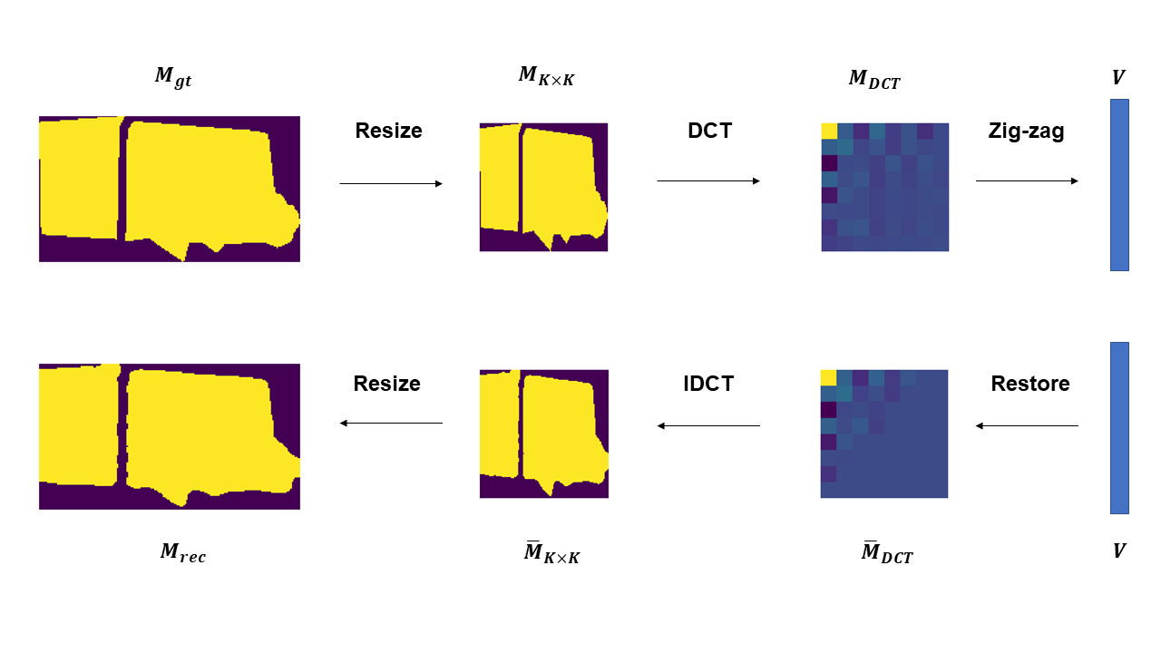
Our method is motivated by the JPEG standard [29], an image file format. The pipeline of DCT mask representation is similar to JPEG which encodes the binary mask into a compact vector. As shown in Figure 2, for binary ground truth mask $M_{gt}\in R^{H\times W}$, where H and W denotes the height and width, respectively. We resize it into $M_{K\times K}\in R^{K\times K}$ with bilinear interpolation where $K\times K$ is the mask size. Throughout this paper, $K=128$. It should be noted that $K=28$ in Mask R-CNN.

Two-dimensional DCT-II transforms $M_{K\times K}$ to the frequency domain $M_{DCT}\in R^{K\times K}$:

$$M {}_{DCT}(u,v)=\frac{2}{K}C(u)C(v)$$

$$\sum_{x=0}^{K-1}\sum_{y=0}^{K-1}M_{K\times K}(x,y)\cos\frac{(2x+1)u\pi}{2K}\cos\frac{(2y+1)v\pi}{2K},$$ (1)

where $C(w)=1/\sqrt{2}$ for $w=0$ and $C(w)=1$ otherwise.

Because of the strong “energy compaction” property of DCT, we select the first N-dimensional vector $V\in R^{N}$ from $M_{DCT}$ in a “zig-zag”. Here the DCT mask vector $V$ is the mask representation we desire.

We restore $\bar{M}_{DCT}\in R^{K\times K}$ from $V$ by filling in the other parts with $0$. The next step is to take the two-dimensional inverse DCT (a 2D type-III DCT):

$$\bar{M}_{K\times K}(x,y)= \frac{2}{K}\sum_{u=0}^{K-1}\sum_{v=0}^{K-1}C(u)C(v)\bar{M}_{DCT}(u,v)$$

$$\cos\frac{(2x+1)u\pi}{2K}\cos\frac{(2y+1)v\pi}{2K},$$ (2)

Finally, the bilinear interpolation is adopted to resize $\bar{M}_{K\times K}$ into $M_{rec}\in R^{H\times W}$.

From the above, we encode the ground truth of mask $M_{gt}$ as a compact vector $V$, then decode $V$ to reconstruct the mask $M_{rec}$. In this way, we use an N-dimensional vector $V$ as mask representation instead of a binary image which significantly reduces the redundancy. From Figure 2, DCT mask representation captures the shape of the object accurately, and the discarded high-frequency component is only a few points from the boundary.

As shown in Table 2, We evaluate the quality of mask representation by the metric of IoU between $M_{gt}$ and $M_{rec}$. DCT mask representation uses 100-dimensional and 700-dimensional vectors to achieve the same IoU as the $28\times 28$ and $128\times 128$ matrices in binary grid mask representation. This shows the efficiency of DCT mask representation. Because the size of most objects is smaller than $256\times 256$ on COCO, the results of $256\times 256$ are close to $128\times 128$. Therefore, $128\times 128$ resolution mask is sufficient for the task of instance segmentation.

Moreover, fast cosine transform (FCT) algorithm [14] computes DCT operations with only $O(nlogn)$ complexity, so the amount of calculation in this part is negligible. DCT can be perfectly integrated into the deep learning framework for training and inference.

In summary, without any pre-processing or pre-training, DCT mask representation effectively captures the details of a mask with low complexity. It casts the task of mask prediction into regressing the DCT vector $V$.

Resolution	Dim	IoU
$28\times 28$	None	0.938
$64\times 64$	None	0.968
$128\times 128$	None	0.980
$128\times 128$	100	0.940
$128\times 128$	300	0.970
$128\times 128$	500	0.976
$128\times 128$	700	0.979
$256\times 256$	100	0.940
$256\times 256$	300	0.970
$256\times 256$	500	0.977
$256\times 256$	700	0.980

Table 2: The quality of DCT mask representation with different dimensions and resolution. “None” stands for the binary grid mask representation.

(a) Mask R-CNN

(b) DCT-Mask R-CNN

Figure 3: The implementation of DCT-Mask on the basis of Mask R-CNN.

3.2 DCT-Mask in Mask R-CNN

We could integrate the DCT-mask into most pixel-based instance segmentation frameworks with slight modifications to the model architecture. In this section, we take Mask R-CNN as an example.

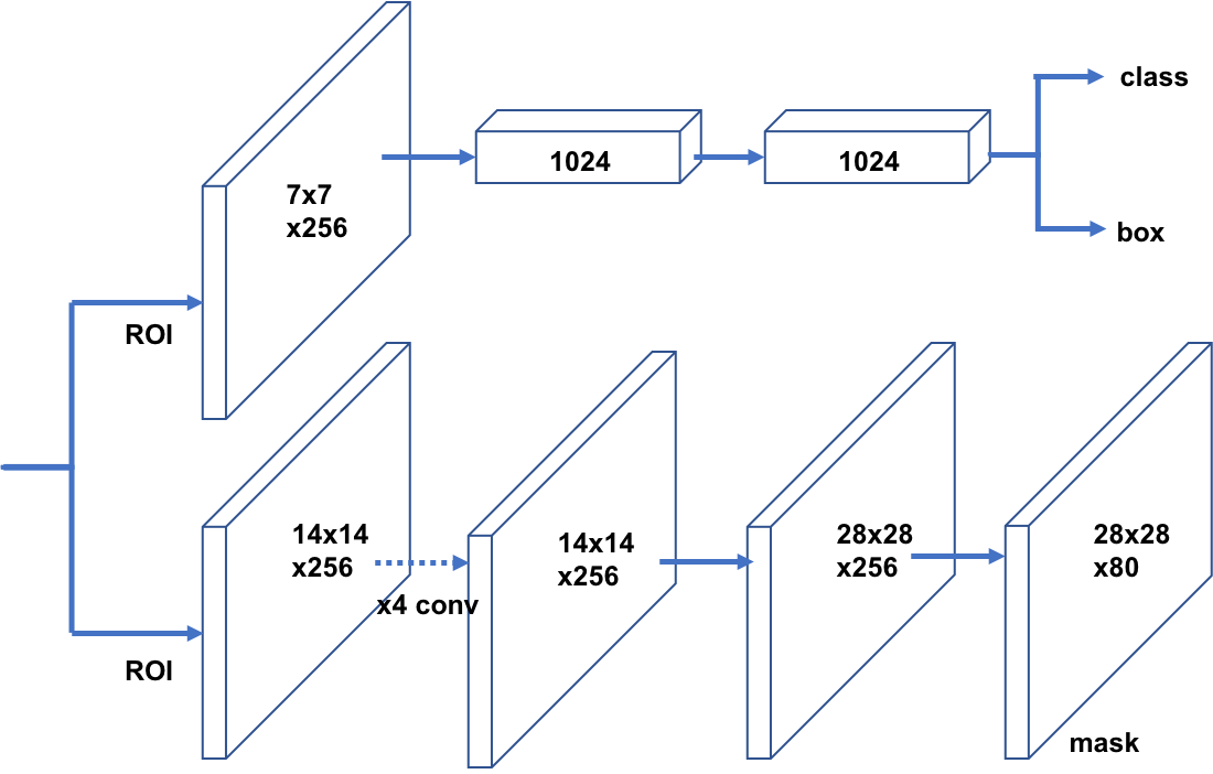
We begin by briefly reviewing the Mask R-CNN [15]. Mask R-CNN is a two-stage instance segmentation method. The first stage generates proposals about the regions by the Region Proposal Network(RPN). The second stage consists of detection branch and mask branch. The detection branch predicts the class of the object and refines the bounding box based on the first stage proposal by R-CNN Head. The mask branch performs pixel classification to generate the mask of the object by mask head.

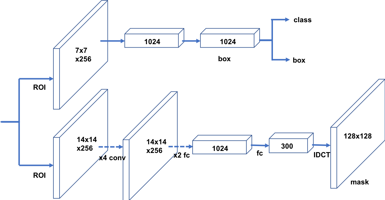
By applying the DCT mask representation, the prediction of the mask branch is a compact vector instead of a binary grid. As shown in Figure 3, we use 4 convolution layers to extract the feature of mask, and 3 fully connected layers to regress the DCT mask vector. The setting of convolution layers is the same as Mask R-CNN where the kernel size and filter number are 3 and 256 respectively. The outputs of the first two fully-connected layers have the size of 1024, and the output size of the last layer is the dimension of the DCT mask vector. Furthermore, the prediction of mask head is class-agnostic which reduces the training complexity by keeping a small output size.

With DCT mask representation, the ground truth of mask branch is a vector encoded by DCT. It leads to a regression problem. Then we define the loss function of mask branch as following:

$$\mathcal{L}_{mask}=\mathtt{1}^{obj}\sum_{i}^{N}D(\hat{V}_{i},V_{i}),$$ (3)

where $V_{i},\hat{V_{i}}$ denotes $i$-th element in ground-truth and prediction vectors, respectively. $\mathtt{1}^{obj}$ is the indicator function for positive samples. $D$ is the distance metric which is $l_{1}$ loss in this article.

We define the loss function of the whole model,

$$\mathcal{L}=\mathcal{L}_{{det}}+\lambda_{{mask}}\cdot\mathcal{L}_{{mask}},$$ (4)

where $\mathcal{L}_{det}$ is the loss for the detection branch. $\lambda_{mask}$ is the corresponding weight.

During inference, we follow the standard Mask R-CNN inference procedure. After NMS, top-k scoring boxes are selected and fed into the Mask branch with RoIAlign. Mask branch predicts a DCT mask vector for each bounding box. The mask within the box is generated by decoding the DCT mask vector.

In summary, keeping the other parts completely unchanged, we only modify the mask branch by replacing the last 2 layers with 3 fully connected layers. Similarly, our method can be easily applied to other pixel-based instance segmentation frameworks

4 Experiments

4.1 Datasets

We evaluate our method on COCO [22] and Cityscapes datasets [10]. We use COCO evaluation metrics AP (averaged over IoU thresholds) to report the results including AP@0.5, AP@0.75, $AP_{S}$, $AP_{M}$, and $AP_{L}$ (AP at different scales).

COCO has 80 categories with instance-level annotation. Following COCO 2017 settings, we train on train2017 (about 118k images) and validate on val2017 (about 5k images). The COCO ground-truth is often too coarse to reflect improvements in mask AP while LVIS [13] re-annotates the COCO dataset with higher quality masks. We use the same models trained on the COCO dataset, and re-evaluate it on the COCO category subset of LVIS, denoted as LVIS^∗.

Cityscapes is a widely used ego-centric street-scene dataset with 2975 training, 500 validation, and 1525 testing images with high-quality annotations. We evaluate the performance in terms of the average precision (AP) metric averaged over 8 semantic classes of the dataset.

4.2 Implementation Details

In this paper, we choose $128\times 128$ mask size and 300-dimensional DCT mask vector as default mask representation. Our method is implemented on both Detectron2 [32] and MMDetection [6], the experimental results of these two toolboxes are consistent. We use the standard $1\times$ training schedule and multi-scale training from Detectron2 by default. On COCO, the experiments adopt 90K iterations, batch size 16 on 8 GPUs, and base learning rate 0.02. The learning rate is reduced by a factor of 10 at iteration 60K and 80K. Multi-scale training is used with shorter side randomly sampled from $[640,800]$. The short side is resized to 800 in inference. On Cityscapes, we use 24K iterations and 0.01 base learning rate, and reduce the learning rate at 18K. Shorter side is randomly sampled from $[800,1024]$ in training, and resized to 1024 in inference.

Loss function and corresponding weight.

(a) Mean

(b) Variance

Figure 4: Mean value and Variance of DCT mask vectors on COCO 2017 val dataset.

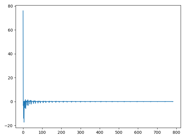
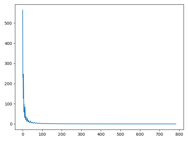
As shown in Figure 4, because of the energy concentration characteristics of DCT, most information concentrates on the previous dimensions. The mean and variance of previous dimensions are much larger than the latter. Hence $l_{2}$ loss would be unstable in the training process. In Table 3, we compare $l_{1}$ loss and smooth $l_{1}$ loss with different corresponding weights $\lambda_{mask}$. It turns out $l_{1}$ and smooth $l_{1}$ have similar performance, and DCT-Mask is robust to the corresponding weight. We choose the best combination of $l_{1}$ loss and $\lambda_{mask}=0.007$ in this paper.

Loss	Weight	COCO AP	LVIS∗ AP
$l_{1}$	0.005	36.2	39.3
	0.006	36.4	39.4
	0.007	36.5	39.6
	0.008	36.2	39.2
smooth $l_{1}$	0.004	36.4	39.1
	0.005	36.4	39.2
	0.006	36.4	39.5
	0.007	36.4	39.3

Table 3: The results of $l_{1}$ loss and smooth $l_{1}$ loss with different corresponding weights. The resolution is $128\times 128$, and the number of dimensions is 300.

Method	COCO						LVIS∗						Cityscapes
	AP	AP@50	AP@75	APS	APM	APL	AP	AP@50	AP@75	APS	APM	APL	AP
Mask R-CNN	35.2	56.3	37.5	17.2	37.7	50.3	37.6	59.2	39.2	21.2	43.7	55.1	33.0
DCT-Mask R-CNN	36.5	56.3	39.6	17.7	38.6	51.9	39.7	59.7	42.1	23.5	46.5	58.5	35.6

Table 4: Mask AP on the validation set of COCO, LVIS^∗ and Cityscapes. ResNet-50 backbone and 1x training schedule are used. The results show that DCT-Mask yields higher AP gains with higher quality annotations.

Method					Backbone	DCT-Mask	COCO		LVIS∗
			AP	AP@50	AP@75	AP	AP@50	AP@75
Mask R-CNN	ResNet-50		35.2	56.3	37.5	37.6	59.2	39.2
		✓	36.5(+1.3)	56.3	39.6	39.7(+2.1)	59.7	42.1
	ResNet-101		38.6	60.4	41.3	41.4	63.0	44.0
		✓	39.9(+1.3)	60.5	43.4	43.7(+2.3)	63.6	46.8
	ResNeXt-101		39.5	61.7	42.6	42.1	63.6	45.0
		✓	41.2(+1.7)	62.4	44.9	45.2(+2.9)	65.7	48.5
Casecade Mask R-CNN	ResNet-50		36.4	56.9	39.2	38.9	59.9	41.2
		✓	37.5(+1.1)	57.0	40.8	40.9(+2.0)	60.1	43.5
	ResNet-101		39.6	60.9	42.9	42.2	63.5	45.3
		✓	40.8(+1.2)	61.5	44.4	44.3(+2.1)	63.8	47.8
	ResNeXt-101		40.2	62.3	43.5	43.2	64.4	46.3
		✓	42.0(+1.8)	63.0	45.8	46.0(+2.8)	66.3	49.5

Table 5: Mask AP on COCO and LVIS^∗ validation dataset with different backbones. The results without ✓are those of standard Mask R-CNN and Cascade Mask R-CNN, while with ✓are those of DCT-Mask. 1x training schedule is used for ResNet-50, 3x training schedule is used for ResNet-101 and ResNeXt-101. The results shows that our method yields higher AP gains with more complex backbones.

4.3 Main Results

We compare DCT-Mask R-CNN to the standard Mask R-CNN with ResNet-50 backbone in Table 4. On the COCO, LVIS^∗, and Cityscapes datasets, mask AP of our method is increased by 1.3%, 2.1%, 2.6% respectively. Especially for AP@75, DCT-Mask outperforms baseline by 2.1% and 2.9% on COCO and LVIS^∗, respectively. Recalling that Cityscapes and LVIS^∗ have higher-quality annotations, which allows them to evaluate mask improvements in more details. DCT-Mask yields more increments in AP_M and AP_L than AP_S, because larger objects need higher-resolution mask representation to capture the details.

DCT mask representation allows our method to yield higher AP with lower FLOPs. As shown in Table 6, compared to Mask R-CNN with $128\times 128$ resolution, our method brings a 3.6% AP gain with more than 20 times less computation (FLOPs). Moreover, DCT-Mask predicts $128\times 128$ resolution masks at 22 FPS which is almost the same as Mask R-CNN with $28\times 28$ resolution.

Theoretically, DCT-Mask can be integrated into most pixel-based instance segmentation frameworks. At Table 5, we show that DCT-Mask achieves consistent performance on Cascade Mask R-CNN[2].

It is worth to mention that our method has a greater improvement for large backbones. We show this property in Table 5. Compared to the standard Mask R-CNN, DCT-Mask respectively increases 1.3% and 1.7% mask AP with ResNet-50 and ResNeXt-101 on COCO 2017 val dataset. On LVIS^∗ dataset, it increases 2.1% and 3.1% mask AP respectively. The same property is also presented on Cascade Mask R-CNN[2]. DCT-Mask respectively increases 1.1% and 1.8% mask AP with ResNet-50 and ResNeXt-101 on COCO, while it increases 2.0% and 2.8% mask AP on LVIS^∗. Because DCT mask representation captures more detailed features and improves the quality of the mask, a larger backbone can make full use of this advantage, thereby further improving the results.

Method	Resolution	AP	FLOPs	FPS
Mask R-CNN	$28\times 28$	35.2	0.5B	23
Mask R-CNN	$64\times 64$	34.4	2.7B	19
Mask R-CNN	$128\times 128$	32.9	11.0B	13
DCT-Mask R-CNN	$128\times 128$	36.5	0.5B	22

Table 6: Mask head FLOPs and FPS for a $128\times 128$ resolution mask. The FPS index is measured on V100. DCT-Mask increases 3.6% AP with 20 times less FLOPs.

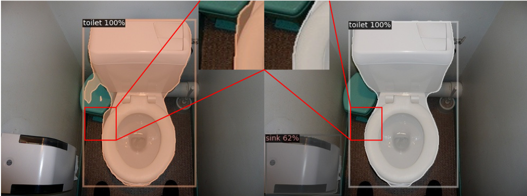
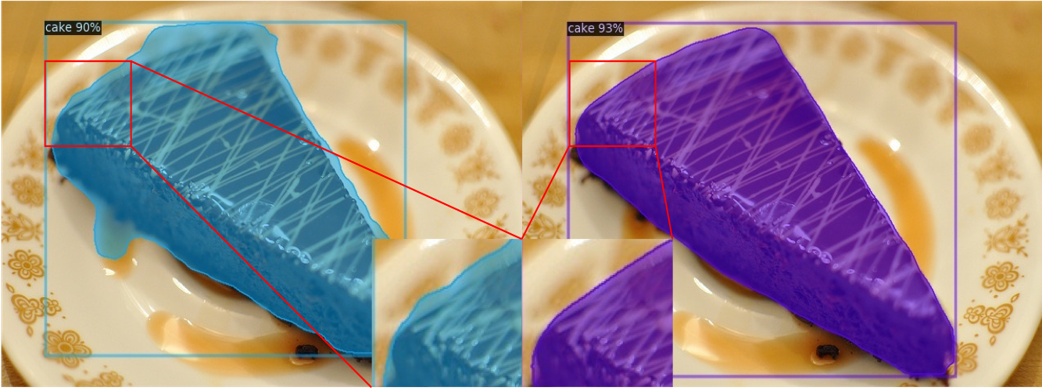
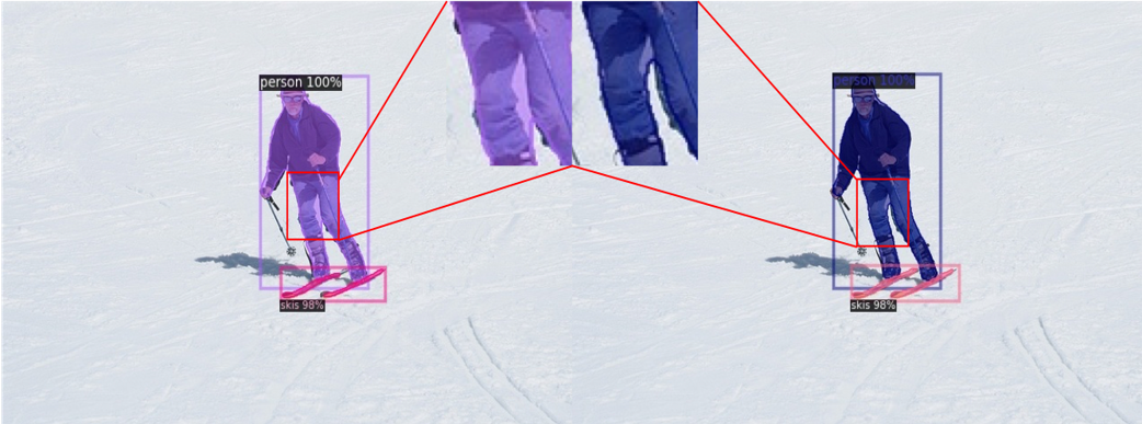
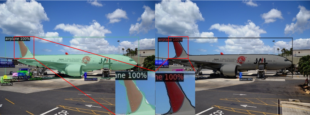
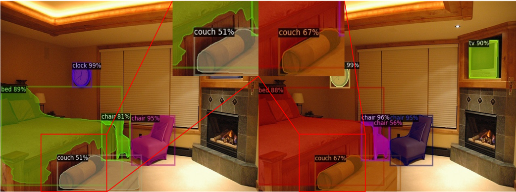
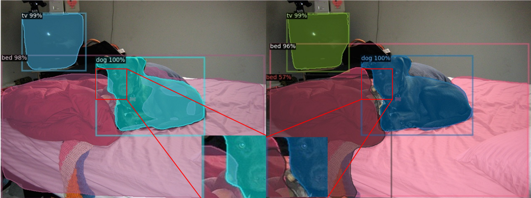
DCT-Mask R-CNN outputs are visualized in Figures 5. Compared to the standard Mask R-CNN, DCT-Mask obtains finer results around object boundaries. Moreover, we compare our method with other instance segmentation methods on COCO test-dev2017 and Cityscapes test at Table 11 and Table 12. Without bells and whistles, DCT-Mask achieves state-of-the-art performances.

4.4 Ablation Study

Resolution	Dim	AP	IoU
$32\times 32$	300	35.4	0.950
$64\times 64$	300	36.4	0.968
$128\times 128$	300	36.5	0.970
$256\times 256$	300	36.5	0.970

Table 7: DCT-Mask with different resolutions. It shows that higher resolution has higher IoU and mask AP.

In this part, we explore the reason why our method increases the mask AP from the perspective of mask quality and model architecture modifications. In these experiments, we use Mask R-CNN framework and ResNet-50 backbone, and evaluate on COCO 2017val dataset.

Resolution of mask representation. DCT mask representation can obtain high-quality mask with low complexity. As shown in Table 7, when the dimension of the DCT vector is the same(Dim=300), as the resolution increases from $32\times 32$ to $128\times 128$, IoU increases from $0.95$ to $0.97$. DCT mask representation captures more information, and mask AP is increased from 35.4 to 36.5. When the resolution increases to $256\times 256$, the mask quality is almost unchanged, mask AP is the same as $128\times 128$.

Dimension of DCT mask vector. Because of the energy concentration characteristics of DCT, the “importance” of the latter dimension is less than the former. This is reflected in the experiments. As illustrated in Table 8, with the same resolution $128\times 128$, as the dimension increases from 100 to 900, the growth of mask quality is gradually slowed. When Dim $>$300, due to the increased training complexity, although the mask quality has improved, mask AP remains basically unchanged.

Resolution	Dim	$AP$	IoU
$128\times 128$	100	35.3	0.940
$128\times 128$	300	36.5	0.970
$128\times 128$	500	36.5	0.976
$128\times 128$	700	36.5	0.979
$128\times 128$	900	36.4	0.980

Table 8: DCT mask vectors with different dimensions. As dimension increases, the growth of IoU is gradually slowed, and mask AP remains basically unchanged when $Dim>300$.

Different representations with the same quality. For a 784-dimensional DCT mask vector of $28\times 28$ resolution, DCT could be regarded as a reversible transformation. It transforms the pixel mask representation into the frequency domain, and the quality of mask representation is the same. Besides, for a 100-dimensional DCT mask vector of $128\times 128$ resolution, the mask quality is $0.94$ which is close to binary mask representation with $28\times 28$ resolution in the standard Mask R-CNN. As shown in Table 9, the performance of these experiments is very close to the Mask R-CNN baseline. This implies that the type of mask representation is not the reason for the increase in mask AP.

In summary of the previous three parts, DCT mask representation of different resolutions with the same mask quality has the same performance. Different types of mask representations with the same mask quality have the same performance. Besides, when mask quality increases as the dimension increases, the mask AP also increases. When mask quality remains basically unchanged as the dimension increases, the mask AP remains unchanged. We can conclude that the increase of mask AP is due to the increase of mask quality, not the type of mask representation. The reason why DCT-Mask works is that it achieves a balance between mask quality and complexity.

Resolution	Dim	AP	IoU
$28\times 28$	None	35.2	0.938
$28\times 28$	784	35.4	0.938
$128\times 128$	100	35.3	0.940

Table 9: Different mask representations with similar mask quality. “None” denotes the binary grid mask representation in standard Mask R-CNN. Mask AP is close with similar mask quality.

The effect of the architecture modifications.

Method				3 FC	L1	AP
Mask R-CNN			34.7
	✓		34.6
	✓	✓	18.5

Table 10: The effect of architecture modifications. The added 3 FC layers shows negligible impact on the results. $l_{1}$ loss is not suitable for Mask R-CNN.

We integrate DCT mask representation into the standard Mask R-CNN with slight modifications to the model architecture. To make sure the improvement of our method is not due to these modifications, we add 3 fully connected(FC) layers and apply $l_{1}$ loss to the standard Mask R-CNN mask branch, respectively. Because the output size of the FC layers is 784, we use the class agnostic mask. As shown in Table 10, the impact of the FC layers could be ignored, and $l_{1}$ loss is not suitable for binary grid mask.

The design of the mask branch. We investigate the impact of the detailed setting of mask branch. As we present before, we use 4 convolution layers and 3 FC layers in mask branch and achieves 36.5 AP on COCO with ResNet-50. We find that adding one more convolution layer or FC layer will achieve 36.4 AP and 36.3 AP respectively. Moreover, when we increase the hidden size of FC layers from 1024 to 2048, it achieves 36.5 AP. It implies that the design of the mask branch is not specific, DCT-Mask is feasible for different setting of mask branch.

Method	Backbone	aug.	sched.	AP	AP@50	AP@75	APS	APM	APL
MEInst[36]	ResNet-101-FPN	✓	3$\times$	33.9	56.2	35.4	19.8	36.1	42.3
TensorMask[8]	ResNet-101-FPN	✓	6$\times$	37.1	59.3	39.4	17.4	39.1	51.6
MaskLab+[7]	ResNet-101-C4	✓	3$\times$	37.3	59.8	39.6	16.9	39.9	53.5
BMask R-CNN [9]	ResNet-101-FPN		1$\times$	37.7	59.3	40.6	16.8	39.9	54.6
MS R-CNN[17]	ResNet-101-FPN		18e	38.3	58.8	41.5	17.8	40.4	54.4
BlendMask[4]	ResNet-101-FPN	✓	3$\times$	38.4	60.7	41.3	18.2	41.5	53.3
Mask R-CNN[15]	ResNet-101-FPN	✓	3$\times$	38.8	60.9	41.9	21.8	41.4	50.5
CondInst[27]	ResNet-101-FPN	✓	3$\times$	39.1	60.9	42.0	21.5	41.7	50.9
SOLOv2[30]	ResNet-101-FPN	✓	6$\times$	39.7	60.7	42.9	17.3	42.9	57.4
HTC[5]	ResNet-101-FPN		20e	39.7	61.8	43.1	21.0	42.2	53.5
HTC	ResNeXt-101-FPN		20e	41.2	63.9	44.7	22.8	43.9	54.6
PointRender[20]	ResNeXt-101-FPN	✓	3$\times$	41.4	63.3	44.8	24.2	43.9	53.2
DCT-Mask R-CNN	ResNet-101-FPN	✓	3$\times$	40.1	61.2	43.6	22.7	42.7	51.8
DCT-Mask R-CNN	ResNeXt-101-FPN	✓	3$\times$	42.0	63.6	45.7	25.1	44.7	53.3
Casecade DCT-Mask R-CNN	ResNet-101-FPN	✓	3$\times$	41.0	61.7	44.7	23.7	43.3	52.6
Casecade DCT-Mask R-CNN	ResNeXt-101-FPN	✓	3$\times$	42.6	64.0	46.4	25.2	45.1	54.3

Table 11: Comparing different instance segmentation methods on COCO 2017 test-dev. “aug.”: using multi-scale data augmentation during training. “sched.”: the used learning rate schedule.

(a)

(b)

Figure 5: Example result pairs from Mask R-CNN vs. with DCT-Mask R-CNN(right image), using ResNet-50 with FPN.

Methods	Backbone	AP	AP50
Mask R-CNN[15]	ResNet-50-FPN	26.2	49.9
BshapeNet+[19]	ResNet-50-FPN	27.3	50.5
BMask R-CNN[9]	ResNet-50-FPN	29.4	54.7
PointRend[20]	ResNet-50-FPN	30.4	55.1
DCT-Mask R-CNN	ResNet-50-FPN	30.6	55.4

Table 12: Comparing different instance segmentation methods on Cityscapes test with only fine annotations.

5 More discussion to prior works

In this section, we investigate relations and differences between DCT-Mask and some prior works.

Comparison with PointRend. PointRend[20] improves the mask representation by iteratively “rendering” the output mask from $7\times 7$ resolution to $224\times 224$, while DCT-Mask directly achieves high resolution by decoding the DCT mask vector. As shown in Table 13, our method achieves slightly better mask AP and outperforms PointRend by lower FLOPs and higher FPS.

Comparison with MEInst. MEInst[36] proposes a one-stage instance segmentation framework based on FCOS, which applies PCA to encode the mask into a compact vector as mask representation. It increases the mask AP by reducing the training complexity with a much smaller compact vector. As we discussed before, mask quality is important to the mask prediction. MEInst only uses a $28\times 28$ resolution mask, and the mask quality drops to 91.5%. We apply PCA to encode the mask with the same setting, which is $128\times 128$ resolution and 300 components. It only achieves 34.8 AP on COCO while DCT achieves 36.5 AP. Moreover, PCA needs extra pre-training. DCT is clearly a better choice for mask encoding.

Method	Resolution	COCO	LVIS∗	FLOPs	FPS
DCT-Mask R-CNN	$128\times 128$	36.5	39.7	0.5B	22
PointRend	$224\times 224$	36.3	39.7	0.9B	16

Table 13: Comparison with PointRend on the COCO 2017val dataset. DCT-Mask outperforms PointRend with lower FLOPs and higher FPS.

6 Conclusion

In this work, we have introduced a simple and effective approach to significantly increase the mask AP of instance segmentation. The increase is due to the high-quality and low-complexity DCT mask representation. DCT-Mask could be easily integrated into most pixel-based methods. We hope our method can serve as a fundamental approach in instance segmentation.

7 Acknowledgements

This work was supported by Alibaba Innovative Research(AIR) Program and Major Scientific Research Project of Zhejiang Lab (No.2019DB0ZX01).

Thank Xue Yang for his insightful help.

References

- [1] Vladimir Britanak, Patrick C Yip, and Kamisetty Ramamohan Rao. Discrete cosine and sine transforms: general properties, fast algorithms and integer approximations. Elsevier, 2010.
- [2] Zhaowei Cai and Nuno Vasconcelos. Cascade r-cnn: Delving into high quality object detection. In Proceedings of the IEEE conference on Computer Vision and Pattern Recognition, pages 6154–6162, 2018.
- [3] Aman R Chadha, Pallavi P Vaidya, and M Mani Roja. Face recognition using discrete cosine transform for global and local features. In 2011 INTERNATIONAL CONFERENCE ON RECENT ADVANCEMENTS IN ELECTRICAL, ELECTRONICS AND CONTROL ENGINEERING, pages 502–505. IEEE, 2011.
- [4] Hao Chen, Kunyang Sun, Zhi Tian, Chunhua Shen, Yongming Huang, and Youliang Yan. Blendmask: Top-down meets bottom-up for instance segmentation. In Proceedings of the IEEE conference on Computer Vision and Pattern Recognition, pages 8573–8581, 2020.
- [5] Kai Chen, Jiangmiao Pang, Jiaqi Wang, Yu Xiong, Xiaoxiao Li, Shuyang Sun, Wansen Feng, Ziwei Liu, Jianping Shi, Wanli Ouyang, et al. Hybrid task cascade for instance segmentation. In Proceedings of the IEEE conference on Computer Vision and Pattern Recognition, pages 4974–4983, 2019.
- [6] Kai Chen, Jiaqi Wang, Jiangmiao Pang, Yuhang Cao, Yu Xiong, Xiaoxiao Li, Shuyang Sun, Wansen Feng, Ziwei Liu, Jiarui Xu, Zheng Zhang, Dazhi Cheng, Chenchen Zhu, Tianheng Cheng, Qijie Zhao, Buyu Li, Xin Lu, Rui Zhu, Yue Wu, Jifeng Dai, Jingdong Wang, Jianping Shi, Wanli Ouyang, Chen Change Loy, and Dahua Lin. MMDetection: Open mmlab detection toolbox and benchmark. arXiv preprint arXiv:1906.07155, 2019.
- [7] Liang-Chieh Chen, Alexander Hermans, George Papandreou, Florian Schroff, Peng Wang, and Hartwig Adam. Masklab: Instance segmentation by refining object detection with semantic and direction features. In Proceedings of the IEEE conference on Computer Vision and Pattern Recognition, pages 4013–4022, 2018.
- [8] Xinlei Chen, Ross Girshick, Kaiming He, and Piotr Dollár. Tensormask: A foundation for dense object segmentation. In Proceedings of the IEEE International Conference on Computer Vision, pages 2061–2069, 2019.
- [9] Tianheng Cheng, Xinggang Wang, Lichao Huang, and Wenyu Liu. Boundary-preserving mask r-cnn. arXiv preprint arXiv:2007.08921, 2020.
- [10] Marius Cordts, Mohamed Omran, Sebastian Ramos, Timo Rehfeld, Markus Enzweiler, Rodrigo Benenson, Uwe Franke, Stefan Roth, and Bernt Schiele. The cityscapes dataset for semantic urban scene understanding. In Proceedings of the IEEE conference on Computer Vision and Pattern Recognition, pages 3213–3223, 2016.
- [11] Jifeng Dai, Kaiming He, and Jian Sun. Instance-aware semantic segmentation via multi-task network cascades. In Proceedings of the IEEE conference on Computer Vision and Pattern Recognition, pages 3150–3158, 2016.
- [12] Max Ehrlich and Larry S Davis. Deep residual learning in the jpeg transform domain. In Proceedings of the IEEE International Conference on Computer Vision, pages 3484–3493, 2019.
- [13] Agrim Gupta, Piotr Dollar, and Ross Girshick. Lvis: A dataset for large vocabulary instance segmentation. In Proceedings of the IEEE conference on Computer Vision and Pattern Recognition, pages 5356–5364, 2019.
- [14] M Haque. A two-dimensional fast cosine transform. IEEE transactions on acoustics, speech, and signal processing, 33(6):1532–1539, 1985.
- [15] Kaiming He, Georgia Gkioxari, Piotr Dollár, and Ross Girshick. Mask r-cnn. In Proceedings of the IEEE international conference on computer vision, pages 2961–2969, 2017.
- [16] Kaiming He, Xiangyu Zhang, Shaoqing Ren, and Jian Sun. Deep residual learning for image recognition. In Proceedings of the IEEE conference on Computer Vision and Pattern Recognition, pages 770–778, 2016.
- [17] Zhaojin Huang, Lichao Huang, Yongchao Gong, Chang Huang, and Xinggang Wang. Mask scoring r-cnn. In Proceedings of the IEEE conference on Computer Vision and Pattern Recognition, pages 6409–6418, 2019.
- [18] Saumya Jetley, Michael Sapienza, Stuart Golodetz, and Philip HS Torr. Straight to shapes: real-time detection of encoded shapes. In Proceedings of the IEEE conference on Computer Vision and Pattern Recognition, pages 6550–6559, 2017.
- [19] Ba Rom Kang, Hyunku Lee, Keunju Park, Hyunsurk Ryu, and Ha Young Kim. Bshapenet: Object detection and instance segmentation with bounding shape masks. Pattern Recognition Letters, 131:449–455, 2020.
- [20] Alexander Kirillov, Yuxin Wu, Kaiming He, and Ross Girshick. Pointrend: Image segmentation as rendering. In Proceedings of the IEEE conference on Computer Vision and Pattern Recognition, pages 9799–9808, 2020.
- [21] Yi Li, Haozhi Qi, Jifeng Dai, Xiangyang Ji, and Yichen Wei. Fully convolutional instance-aware semantic segmentation. In Proceedings of the IEEE conference on Computer Vision and Pattern Recognition, pages 2359–2367, 2017.
- [22] Tsung-Yi Lin, Michael Maire, Serge Belongie, James Hays, Pietro Perona, Deva Ramanan, Piotr Dollár, and C Lawrence Zitnick. Microsoft coco: Common objects in context. In European conference on computer vision, pages 740–755. Springer, 2014.
- [23] Shu Liu, Lu Qi, Haifang Qin, Jianping Shi, and Jiaya Jia. Path aggregation network for instance segmentation. In Proceedings of the IEEE conference on Computer Vision and Pattern Recognition, pages 8759–8768, 2018.
- [24] Shao-Yuan Lo and Hsueh-Ming Hang. Exploring semantic segmentation on the dct representation. In Proceedings of the ACM Multimedia Asia, pages 1–6. 2019.
- [25] K Ramamohan Rao and Ping Yip. Discrete cosine transform: algorithms, advantages, applications. Academic press, 2014.
- [26] Daniele Ravì, Miroslaw Bober, Giovanni Maria Farinella, Mirko Guarnera, and Sebastiano Battiato. Semantic segmentation of images exploiting dct based features and random forest. Pattern Recognition, 52:260–273, 2016.
- [27] Zhi Tian, Chunhua Shen, and Hao Chen. Conditional convolutions for instance segmentation. arXiv preprint arXiv:2003.05664, 2020.
- [28] Matej Ulicny and Rozenn Dahyot. On using cnn with dct based image data. In Proceedings of the 19th Irish Machine Vision and Image Processing conference IMVIP, 2017.
- [29] Gregory K Wallace. The jpeg still picture compression standard. IEEE transactions on consumer electronics, 38(1):xviii–xxxiv, 1992.
- [30] Xinlong Wang, Rufeng Zhang, Tao Kong, Lei Li, and Chunhua Shen. Solov2: Dynamic and fast instance segmentation. Advances in Neural Information Processing Systems, 33, 2020.
- [31] Jie Wei. Image segmentation based on situational dct descriptors. Pattern Recognition Letters, 23(1-3):295–302, 2002.
- [32] Yuxin Wu, Alexander Kirillov, Francisco Massa, Wan-Yen Lo, and Ross Girshick. Detectron2. https://github.com/facebookresearch/detectron2, 2019.
- [33] Enze Xie, Peize Sun, Xiaoge Song, Wenhai Wang, Xuebo Liu, Ding Liang, Chunhua Shen, and Ping Luo. Polarmask: Single shot instance segmentation with polar representation. In Proceedings of the IEEE conference on Computer Vision and Pattern Recognition, pages 12193–12202, 2020.
- [34] Saining Xie, Ross Girshick, Piotr Dollár, Zhuowen Tu, and Kaiming He. Aggregated residual transformations for deep neural networks. In Proceedings of the IEEE conference on Computer Vision and Pattern Recognition, pages 1492–1500, 2017.
- [35] Kai Xu, Minghai Qin, Fei Sun, Yuhao Wang, Yen-Kuang Chen, and Fengbo Ren. Learning in the frequency domain. In Proceedings of the IEEE conference on Computer Vision and Pattern Recognition, pages 1740–1749, 2020.
- [36] Rufeng Zhang, Zhi Tian, Chunhua Shen, Mingyu You, and Youliang Yan. Mask encoding for single shot instance segmentation. In Proceedings of the IEEE conference on Computer Vision and Pattern Recognition, pages 10226–10235, 2020.