Shaping the autocorrelation and photon statistics
Abstract
We propose a method of arbitrarily shaping and scaling the temporal intensity correlations of an optical signal locally, avoiding periodic correlations. We demonstrate our approach experimentally using stochastic intensity modulation. We also analyze and simulate shaping both temporal correlations and photon statistics that are fully specified by the user. We show that within the confines of monotony and convexity, the temporal correlations are independent of photon statistics and can take any shape.
I Introduction
This article focuses on the temporal correlations of optical intensity , conventionally described by the second-order coherence function
| (1) |
which we refer to as intensity autocorrelation. In the quantum realm, it is defined by the means of normally ordered photon-number operators [1]
| (2) |
This article proposes methods of shaping the autocorrelation in an arbitrary way. A straightforward approach would be modulating a pulse train coming from a laser, however pulsed signals have periodic autocorrelation. Our goal is to emulate fluctuating signals exhibiting that approaches unity in the limit of . Any significant deviation from unity is therefore local.
The modulation of optical intensity in time can be used to generate pseudothermal light. A common technique is collecting speckles from light diffused by a rotating ground glass plate [2]. Chaotic light can be also generated by amplified spontaneous emission [3] or direct laser modulation [4]. The resulting photon bunching of can be exploited in classical ghost imaging [5, 6, 7], two-photon-excited fluorescence [8], optical time-domain reflectometry [9], and laser ranging [10].
Shaping the autocorrelation—and thus the spectrum—of a signal is a problem that has been addressed in other fields of signal processing and simulation using various methods [11, 12]. A prominent case is transforming an electronic Gaussian noise by a linear filter and a nonlinear function to obtain a given spectrum and marginal distribution [13]. An alternate solution was proposed in terms of reshuffling of signal samples [14].
In the first part of this article, we present a method of shaping the autocorrelation that exploits stochastic pulse superposition. The spectral properties of such random pulses have been studied in communication theory [15]; we make use of these properties from the perspective of signal generation.
In the second part, we utilize another method of stochastic modulation—random switching of intensity levels that was proposed in Ref. [16]—to shape both temporal correlations and photon statistics. We combine this approach with the photon-statistics-generation algorithm proposed in Ref. [17]. Using numerical simulations, we demonstrate the generation of arbitrarily specified and photon-number distribution. We also analyze the properties and limitations of the method.
II Arbitrary autocorrelation
II.1 Method
The basic premise is that the intensity signal consists of a random Poissonian sequence of non-negative integrable hill functions . Mathematically, the signal is expressed as a sum
| (3) |
The sequence of positions in time follows a homogeneous Poisson point process with a mean rate . This means that every delay is a realization of a random variable with a probability density
| (4) |
The hill function is chosen so that it has a specific cross-correlation , while its norm may be arbitrary. The terms are defined as
| (5) | ||||
| (6) |
where the cross-correlation observes . Then, the intensity autocorrelation of becomes
| (7) |
The proof is given in Appendix A. The autocorrelation shape is therefore given solely by the shape of , the amplitude of which may be arbitrary. The and the scale of the whole autocorrelation can be set by the rate .
Given a specific , one can obtain the hill function using Fourier transforms (see Appendix B),
| (8) | ||||
| (9) |
For any consistent with (1), the function is real and non-negative by virtue of the Wiener-Khinchin theorem. The sign function in (9) is any piecewise function yielding . The constraint of this method is that the needs to be given so that there exists a sign function that results in a non-negative .
Superposition
A generalization of this approach allows generating a superposition of multiple shapes by randomly alternating between hill functions. Suppose a set of hill functions with respective cross-correlations appearing with probabilities , but sharing the same mean frequency . The calculation of is a straightforward extension, yielding
| (10) |
Background
If we consider a background offset so that , the mean value of the signal is and the signal-to-noise ratio between and becomes a factor that scales down the intensity autocorrelation:
| (11) |
The maximum bunching possible is achieved for .
Non-overlapping hills
In a particular experimental realization—such as presented here—it may not be possible to generate a mathematical superposition of the hill functions. For example, a function generator can only produce one pulse at a time and so the hills cannot overlap. In such cases, the hill function is defined on a finite support and the minimum distance between the hills’ peaks is . Consequently, the cross-correlation is only nonzero for , and the unity term in (7) becomes locally distorted. The expression changes to (see Appendix C)
| (12) | ||||
II.2 Results
| Shape | |||||||||||||
|---|---|---|---|---|---|---|---|---|---|---|---|---|---|
| Gauss | 2 | ||||||||||||
| Cauchy–Lorentz | 3 | ||||||||||||
| Hyperb. secant | 5 | ||||||||||||
|
|
|
3 | ||||||||||
| Nonmonotone |
|
|
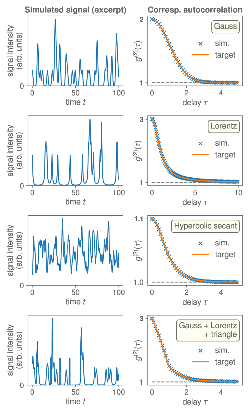
The method of stochastic signal generation is simulated in Fig. 1. For illustrative purposes, the signals are shown for both high and low intensities , respectively corresponding to low and high values of . A mixture of three shapes corresponding to (10) is given in the last row.
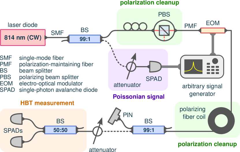
Experimental evidence was obtained using the measurement setup depicted in Fig. 2. The source was a single-mode-fiber-coupled (SMF) continuous-wave laser diode at 814 nm. The optical signal was coupled into a polarization-maintaining fiber (PMF) using a manual polarization controller and a polarizing beam splitter (PBS). The intensity of the signal was modulated by an integrated electro-optical Mach-Zehnder modulator (EOM; EOSpace). The modulator was driven by an arbitrary signal generator (Tektronix) programed to emit a voltage pulse upon each triggering event, which was fed into the fast radio-frequency input of the EOM, having the shape
| (13) |
where the hill is scaled so that , and is the EOM half-wave voltage. The induced transmission modulation is equal to due to the cosine response of the EOM. We assume that the constant bias voltage of the EOM is set precisely to the zero-level transmission. The triggering came from a single-photon avalanche diode (SPAD) illuminated by a constant intensity that was set to a mean count rate . This served as the source of Poissonian events. The output was split between a p-i-n diode and a single-photon Hanbury-Brown–Twiss (HBT) measurement [1]. The p-i-n served for live monitoring of the output and the HBT configuration measured the . For all measurements, the minimum pulse-to-pulse delay was µs. It means that the triggering SPAD dead time of 29 ns could be safely neglected. The data from the SPADs were acquired by a 81-ps time-tagging unit (qutools), the coincidence window for the HBT autocorrelation measurement was 10 ns, and the measurement time was 100 s for each set.
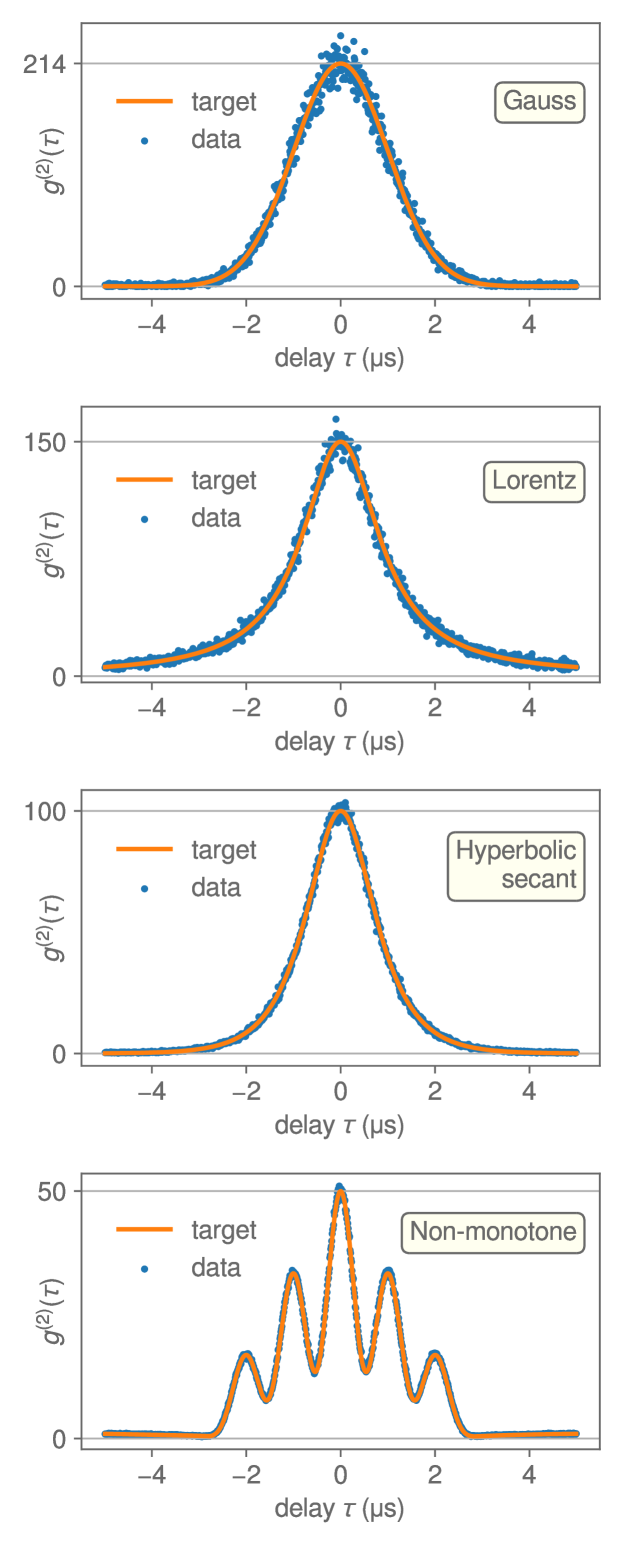
The results of the HBT measurement are shown in Fig. 3. The Gaussian autocorrelation was set to the highest possible amplitude achievable for the Gaussian, , which corresponds to a modulation dynamic range 30.8 dB; the others were set to round values 50, 100, and 150. The modulation scheme corresponds to the non-overlapping scenario with the expected autocorrelation given by (12), where the effect of non-unity background is small compared to the overall amplitude [18].
The limiting factor for autocorrelation speed is the 225-MHz bandwidth of the arbitrary signal generator. The limiting factor for the amplitude is the dynamic range of the modulation. It is reduced by thermally induced phase drifts in the EOM, by the polarization extinction ratio, by the EOM interferometric visibility, and by the detectors’ dark count rate. Consequently, the dynamic range determines the maximum bunching achievable for each autocorrelation shape (Gaussian, Lorentz, etc.), as given by the optimal rate in (11). For a more detailed discussion of the shapes and maximum bunching, see Appendix A.
III Photon statistics and autocorrelation
There is a possibility of tailoring both temporal autocorrelation and photon (intensity) statistics simultaneously and independently. The technique relies on random switching between intensity levels. This approach was proposed by Pandey et al. [16] who demonstrated the generation of gamma-distributed intensity and exponential autocorrelation shapes. In order to reach arbitrary classical photon statistics, we employ an inversion algorithm proposed in our earlier work [17]. We present an analysis of the limitations and possibilities of the resulting approach and we perform numerical simulations [18].
The optical signal consists of a sequence of intensity levels , each being held for a respective time period . Each and is an independent realization of the corresponding random variable, following the probability density functions and .
The autocorrelation is then given as [16] (see Appendix D)
| (14) | ||||
| (15) |
The averaging terms are always taken over the corresponding distributions— or . The bunching factor (15) is solely given by intensity statistics—as it needs to be—while the temporal shape is given by . To establish the set of possible shapes, let us look at the derivatives
| (16) | ||||
| (17) |
The above inequalities follow from and the non-negativity of . Both inequalities mean that the class of practicable autocorrelation functions is restricted to monotonically non-increasing convex functions for which and the limit . As is proven in Appendix E, any such autocorrelation can be generated by this method.
These conditions are more restrictive than the hill-superposition approach above, as for example all functions in Figs. 1 and 3 are nonconvex and therefore inaccessible. However, we gain the possibility to shape the photon statistics independently.
Photon statistics is given by the integrated intensity
| (18) |
taken over a time interval [19]. Let us consider the units of to be the average number of photons per time, meaning that is dimensionless. The number of photons detected inside a time interval follows the probability distribution given by Mandel’s formula [19]
| (19) |
In order to have control over the photon statistics, the distribution needs to follow , ideally when , implying . This can be achieved either in the limit of a short time window , or if the intensity switching is synchronized with the time windows. The latter implies that the window length becomes an elementary time unit of the modulation, and the autocorrelation is restricted to a piecewise linear function with the resolution . This case corresponds to our discrete numerical simulations.
Following the approach presented in Ref. [17], we take a finite set and construct a matrix . Each has a corresponding probability . The Mandel formula (19) then becomes
| (20) |
where the vector needs to be solved for a given photon statistics . Suitable sampling and non-negative least squares were shown to work for classical photon statistics [17, 18]. The solution for is discrete: .
Let us now explicitly outline the problem inversion and generation of the random samples of and . We are given the target and . If is a classical photon statistics, then by definition it is achievable by sampling a certain . If the technical limitations of the experiment only allow discrete intensities , we perform a non-negative least-squares inversion of (20) to obtain . In each modulation step, we can randomly choose the intensity using a uniformly distributed random floating-point number by finding the smallest such that [18]. This way, follows the distribution .
To shape the autocorrelation, we establish a survival function using the first derivative ,
| (21) |
In each step, we obtain the hold-off time from a uniformly distributed number using the inverse function that always exists,
| (22) |
Consequently, follows the probability density . The proof of existence and derivations are given in Appendix E.
| Simulation 1 | ||
|---|---|---|
| Simulation 2 |
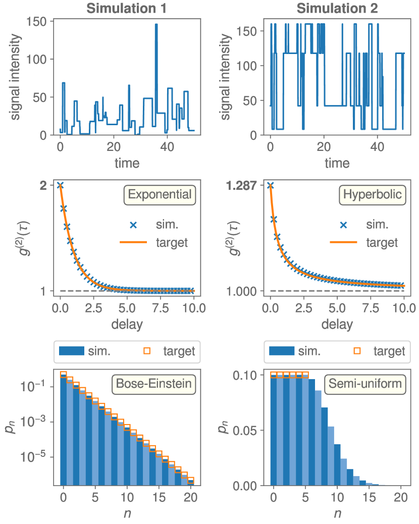
Figure 4 shows two numerically simulated signals that follow certain prescribed autocorrelations and photon statistics. Both signals observe their corresponding , but have different approaches to . Signal 1 takes samples from a continuous exponential distribution, whereas signal 2 follows a discrete solution of (20) for a partially uniform photon statistics . The corresponding prescriptions are given in Table 2.
IV Conclusion
We demonstrated two methods of shaping the autocorrelation of optical intensity. The first allows for more arbitrary shapes; the second is limited to nonincreasing convex functions, but allows tailoring the intensity and photon statistics as well.
Primarily, we consider our contribution to address a fundamental problem in optical signal generation. However, possible practical uses involve exciting or probing systems sensitive to photon correlations [20, 21]. The modulation techniques may also serve to simulate optical fading channels and atmospheric scintillation [22], especially if certain power spectra are required [23, 24, 25]. Atmospheric turbulence has a critical impact on both satellite-based [26, 27] and ground-to-ground [28, 29, 30, 31] quantum communications. Especially, single-mode coupling of atmospheric channels results in significant transmission and phase fluctuations. The proposed methods allow simulation of the channel transmission. The specific properties that can be reproduced are the fading distribution and temporal correlations.
Acknowledgements.
This research has been supported by QuantERA ERA-NET Cofund in Quantum Technologies, EU Horizon 2020, and Ministry of Education, Youth and Sports of the Czech Republic (Project HYPER-U-P-S, No. 8C18002). M. J. also acknowledges the support of the Czech Science Foundation (Grant No. 19-19189S).Appendix A Derivation of autocorrelation of stochastic hill superposition
Let the “hill” function be and its unnormalized cross-correlation function
| (23) |
We are going to consider the intensity of light as a sum of hills randomly distributed in time:
| (24) |
where the peaks follow a homogeneous Poisson point process in time with a mean frequency . This means that peak-to-peak distances follow a negative-exponential probability density distribution . The normalized intensity autocorrelation function is
| (25) |
Let us consider that the intensity signal was generated in a time span and assume the limit of long in our calculations. Then, the number of hills is . We can also denote the integral
| (26) |
which also means . The averaging terms can be calculated simply using the linearity of integration,
| (27) | ||||
| (28) | ||||
where are distances between any two peaks. The sum has terms that can be reduced by considering and :
| (29) | ||||
The peak locations are determined by sampling a random Poisson process and we sum over a large set of samples . We can therefore approximate the above sum by
| (30) |
where the averaging follows a certain probability distribution of distances between any two different peaks. Let us now calculate this distribution. By virtue of the homogeneous Poisson process, we may consider any two different points in time independent with respect to the random occurrence of samples. This allows us to define the average density of peaks per time, which is constant: . Then, the density of peak pairs per distance is
| (31) |
while the corresponding probability density distribution follows by normalizing
| (32) |
Now we can make use of this distribution to calculate (30). Because we assume that time is much longer than both the width of and delay , we can either neglect the linear term in (32) or integrate by parts and approximate the primitive function of by a step function. In any way, we get
| (33) |
Finally, after substituting the rest, we get the final result for the normalized autocorrelation of the randomly generated signal
| (35) |
where is the normalized cross-correlation of . We can see that the shape of does not depend on the amplitude of , only on its shape. The scaling of the is determined solely by the mean frequency .
Factoring in the background is a straightforward extension to the calculations above, yielding (11). After maximizing with respect to , we get the maximum bunching
| (36) |
Let us formulate the dynamic range of the modulation as
| (37) |
which makes sense in the limit of high extinction and , where the hills are far apart and peak value of the hill function effectively represents the maximum intensity that needs to be generated. Then, we can rewrite (36) as
| (38) |
The shape of the autocorrelation is given by , which is given by . Let us define that two autocorrelations and have the same shape if and only if they are identical up to scaling factors and ,
| (39) |
When considering the maximum vertical scale (38), it can be shown that it is invariant under horizontal scaling while keeping the dynamic range constant. One can easily check this by substituting into (5), (6), and (38). Thus we can conclude that the maximum bunching is limited by the modulation dynamic range and by the shape of the autocorrelation. Some examples are given in Table 3.
| Gauss | |
|---|---|
| Cauchy–Lorentz | |
| Hyperb. secant | |
| Triangle |
Appendix B Obtaining the hill shape from autocorrelation
Let us have a given autocorrelation function by specifying (35) numerically or analytically. Our task is to determine and , which together define the desired signal. We use the property of the Fourier transform of a cross-correlation, . Therefore, we can obtain
| (40) |
where the sign function is a piecewise . Because the hill scale is arbitrary, we can simply assign and scale the resulting .
The existence of a precise solution depends on two conditions. The Fourier transform of the cross-correlation and the result must both be non-negative. The non-negativity of is not a restrictive condition, because any legal that can arise from (1) automatically complies due to the Wiener-Khinchin theorem. The positivity of the resulting can sometimes be ensured using a suitable sign-function—a good example is a triangular resulting in a rectangular .
If the autocorrelation is given numerically, we can employ discrete Fourier transform (DFT) defined by relations
| (41) | ||||
| (42) |
Let us consider a given discrete series that defines the autocorrelation symmetrically around zero with a sampling interval ,
| (43) |
Then, we can approximate the Fourier transform
| (44) | ||||
| (45) |
This way, we obtain the discrete Fourier transform with a sampling period . We proceed and get a discrete version of (40),
| (46) |
If we consider the periodicity of DFT, we know that and we can map the implicit range to and obtain the hill function
| (47) |
Appendix C Derivation of nonoverlapping hills
For high bunching, when the mean delay is much greater than the width of the autocorrelation, the signal approaches a sequence of randomly distributed, but disjoint pulses . If a pulse generator is used, it cannot typically generate overlapping signals, which creates a distortion in the . If is defined for , the minimum delay can be . This means that the peaks no longer follow a Poisson process, but a self-excited point process. The limitation of is akin to nonparalyzable dead time of particle detectors.
The distribution of peak pairs becomes more complicated. The term in (29) that sums all the pairs needs to be evaluated separately for immediate neighbors, next-but-one neighbors, and so on. This is because the distribution of must be calculated for each ,
| (48) | ||||
The first step is to consider the sequential delays . By definition, these are independent realizations of a random Poisson process with an addition of . Therefore the probability density function is a shifted negative exponential
| (49) |
Now, considering that , the constituent delays are mutually independent with known distributions. That means that the result has a known distribution. By further induction, as more independent terms are added, we can average over them in each step,
| (50) |
where in means , describing its distribution over all for .
As we assume the limit of long signals, but are interested in finite delays, let us fix and calculate the limit . After substitution of into (48), the averaged terms become
| (51) |
Now let us recall that has a finite support and so for indices , the first term during the whole integration for both plus and minus signs. This means that for each finite , the number of nonzero terms in (48) is finite. As a result, for each . Also note that . The result then is
| (52) |
This result also trivially holds for the case when the minimum delay is , but the support of is narrower. Moreover, the formula can also be adopted for the case of infinite support of and with a minimum delay . In that case, both the sum and the integral would go to infinity; otherwise, the formula would be the same. The only difference in the derivation would be in proving the limit in (48),
| (53) |
As must be integrable, its tail scales faster than . From (51) and the integrability of the gammalike kernel, it follows that from a certain , the term decreases faster than , which means that the limit of the series is zero.
Appendix D Derivation of random switching of intensity levels
The signal is now defined as a step function, where each intensity level is held for a time period . Each of these variables is independently governed by its probability density , . Let us denote averaging over these distributions by unmarked angle brackets , where the distribution is determined by the random variable inside. Averaging over time will be marked by . If we denote the overall number of steps as and the overall time as , we get the mean intensity,
| (54) |
This result easily follows from the uncorrelation of and . However, more discussion is needed for the autocorrelation term.
We express the integral as a sum over the steps again, but the term depends on the delay being greater or smaller than the step width ,
| (55) |
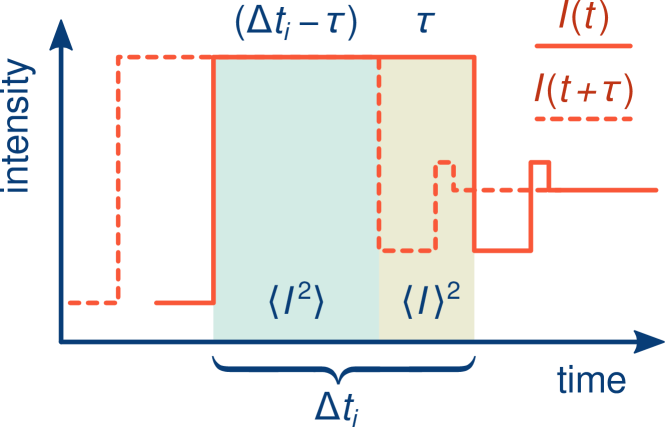
The case of is illustrated in Fig. 5. The area on the left corresponds to the overlap where both signals have the intensity . The area on the right is a product of and the random intensity levels in that follow the th level. We can express this integral overlap as , where is the average intensity of in the area of width . If , the th step has zero overlap with itself and only one term remains.
Now, if we consider the summation over , we may again replace it with averaging over and independently. What is more, the variable gets averaged independently of , because the intensity levels are mutually uncorrelated as well. Therefore , , and . However, the averaging over needs to be split due to the piecewise definition in (55). We obtain
| (56) |
After extending the second integral to infinity to obtain the term and subtracting this extension from the integral on the left, we get
| (57) |
Appendix E Existence of a solution for random intensity levels
The necessary conditions are that the given autocorrelation is continuous, bounded ( and ), monotone, and convex. We claim that these conditions are also sufficient for the existence of a solution. We are going to simplify the notation of the autocorrelation and its derivatives to .
First, we propose that
| (58) |
Because we know that is monotone (convexity of ) and upper bounded (), there must be a limit due to the monotone convergence theorem. We can prove by contradiction that the limit is zero.
Let us assume that , where . Then there exists such that . We can formulate the inequality
| (59) | ||||
| (60) |
This divergence is in conflict with the existence of a converging primitive function , where . Because obviously cannot be positive (), and the limit (58) is proven.
Using Eqs. (16) and (17), we see that the probability density can be expressed as
| (61) |
The initial conditions () mean that is non-negative and owing to (58), it is also normalized,
| (62) |
The only assumption that is left to prove is that the mean value is finite. To this end, we need to establish a survival function as an alternative to the probability density,
| (63) |
A fundamental property of the survival function is
| (64) |
as well as its image . The image is satisfied for all owing to (63) and (58).
The standard formula for the mean value is
| (65) |
However, the survival function offers an alternative [32],
| (66) |
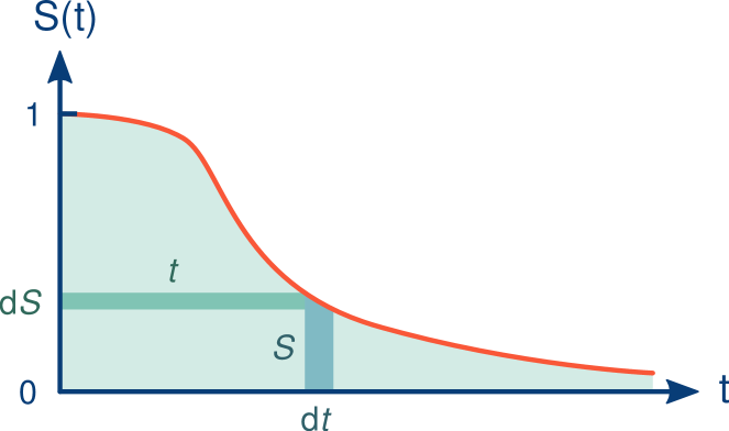
The equivalence of these formulas is illustrated in Fig. 6 and proven by the following:
| (67) | ||||
| (68) |
In the first step, we switch to integration of horizontal slices . Then, we change the integration variable , substitute (64), and arrive at (65). The integrability of follows from (63) and the properties of . We therefore obtain a finite mean value
| (69) |
In conclusion, we have proved the existence of a solution—a valid finite-mean probability distribution of —for every monotone, convex, and appropriately bounded .
References
- Loudon [2000] R. Loudon, The Quantum Theory of Light, 3rd ed. (Oxford University Press, Oxford, U.K., 2000).
- Martienssen and Spiller [2005] W. Martienssen and E. Spiller, Coherence and Fluctuations in Light Beams, American Journal of Physics 32, 919 (2005).
- Boitier et al. [2009] F. Boitier, A. Godard, E. Rosencher, and C. Fabre, Measuring photon bunching at ultrashort timescale by two-photon absorption in semiconductors, Nature Physics 5, 267 (2009).
- Nazarathy et al. [1989] M. Nazarathy, S. A. Newton, R. P. Giffard, D. S. Moberly, F. Sischka, W. R. Trutna, and S. Foster, Real-time long range complementary correlation optical time domain reflectometer, Journal of Lightwave Technology 7, 24 (1989).
- Bennink et al. [2002] R. S. Bennink, S. J. Bentley, and R. W. Boyd, ``Two-Photon” Coincidence Imaging with a Classical Source, Physical Review Letters 89, 113601 (2002).
- Gatti et al. [2004] A. Gatti, E. Brambilla, M. Bache, and L. A. Lugiato, Ghost Imaging with Thermal Light: Comparing Entanglement and ClassicalCorrelation, Physical Review Letters 93, 093602 (2004).
- Zhou et al. [2017] Y. Zhou, F.-l. Li, B. Bai, H. Chen, J. Liu, Z. Xu, and H. Zheng, Superbunching pseudothermal light, Physical Review A 95, 053809 (2017).
- Jechow et al. [2013] A. Jechow, M. Seefeldt, H. Kurzke, A. Heuer, and R. Menzel, Enhanced two-photon excited fluorescence from imaging agents using true thermal light, Nature Photonics 7, 973 (2013).
- Wang et al. [2008] Y. Wang, B. Wang, and A. Wang, Chaotic Correlation Optical Time Domain Reflectometer Utilizing Laser Diode, IEEE Photonics Technology Letters 20, 1636 (2008).
- Lin and Liu [2004] F.-Y. Lin and J.-M. Liu, Chaotic lidar, IEEE Journal of Selected Topics in Quantum Electronics 10, 991 (2004).
- Kim et al. [2010] J. S. Kim, Y. Huh, and M. W. Suh, A method to generate autocorrelated stochastic signals based on the random phase spectrum, Journal of the Textile Institute 101, 471 (2010).
- Müller et al. [2012] C. Müller, C. R. Rojas, and G. C. Goodwin, Generation of amplitude constrained signals with a prescribed spectrum, Automatica 48, 153 (2012).
- Liu and Munson [1982] B. Liu and D. Munson, Generation of a random sequence having a jointly specified marginal distribution and autocovariance, IEEE Transactions on Acoustics, Speech, and Signal Processing 30, 973 (1982).
- Hunter and Kearney [1983] I. W. Hunter and R. E. Kearney, Generation of random sequences with jointly specified probability density and autocorrelation functions, Biological Cybernetics 47, 141 (1983).
- Leneman [1967] O. A. Z. Leneman, Correlation Function and Power Spectrun of Randomly Shaped Pulse Trains, IEEE Transactions on Aerospace and Electronic Systems AES-3, 774 (1967).
- Pandey et al. [2014] D. Pandey, N. Satapathy, B. Suryabrahmam, J. S. Ivan, and H. Ramachandran, Classical light sources with tunable temporal coherence and tailored photon number distributions, European Physical Journal Plus 129, 115 (2014).
- Straka et al. [2018] I. Straka, J. Mika, and M. Ježek, Generator of arbitrary classical photon statistics, Optics Express 26, 8998 (2018).
- Straka and Ježek [2020] I. Straka and M. Ježek, Shaping the autocorrelation and photon statistics, Code Ocean (2020), doi: 10.24433/CO.4221408.v1.
- Mandel and Wolf [1995] L. Mandel and E. Wolf, Optical Coherence and Quantum Optics (Cambridge University Press, Cambridge, U.K., 1995).
- Kazimierczuk et al. [2015] T. Kazimierczuk, J. Schmutzler, M. Aßmann, C. Schneider, M. Kamp, S. Höfling, and M. Bayer, Photon-Statistics Excitation Spectroscopy of a Quantum-Dot Micropillar Laser, Physical Review Letters 115, 027401 (2015).
- Spasibko et al. [2017] K. Yu. Spasibko, D. A. Kopylov, V. L. Krutyanskiy, T. V. Murzina, G. Leuchs, and M. V. Chekhova, Multiphoton Effects Enhanced due to Ultrafast Photon-Number Fluctuations, Physical Review Letters 119, 223603 (2017).
- Vasylyev et al. [2016] D. Vasylyev, A. A. Semenov, and W. Vogel, Atmospheric Quantum Channels with Weak and Strong Turbulence, Physical Review Letters 117, 090501 (2016).
- Dravins et al. [1997] D. Dravins, L. Lindegren, E. Mezey, and A. T. Young, Atmospheric intensity scintillation of stars, i. statistical distributions and temporal properties, Publications of the Astronomical Society of the Pacific 109, 173 (1997).
- Toyoshima et al. [2011] M. Toyoshima, H. Takenaka, and Y. Takayama, Atmospheric turbulence-induced fading channel model for space-to-ground laser communications links, Optics Express 19, 15965 (2011).
- Shen et al. [2014] H. Shen, L. Yu, and C. Fan, Temporal spectrum of atmospheric scintillation and the effects of aperture averaging and time averaging, Optics Communications 330, 160 (2014).
- Liao et al. [2018] S.-K. Liao, W.-Q. Cai, J. Handsteiner, B. Liu, J. Yin, L. Zhang, D. Rauch, M. Fink, J.-G. Ren, W.-Y. Liu, Y. Li, Q. Shen, Y. Cao, F.-Z. Li, J.-F. Wang, Y.-M. Huang, L. Deng, T. Xi, L. Ma, T. Hu, L. Li, N.-L. Liu, F. Koidl, P. Wang, Y.-A. Chen, X.-B. Wang, M. Steindorfer, G. Kirchner, C.-Y. Lu, R. Shu, R. Ursin, T. Scheidl, C.-Z. Peng, J.-Y. Wang, A. Zeilinger, and J.-W. Pan, Satellite-Relayed Intercontinental Quantum Network, Physical Review Letters 120, 030501 (2018).
- Yin et al. [2020] J. Yin, Y.-H. Li, S.-K. Liao, M. Yang, Y. Cao, L. Zhang, J.-G. Ren, W.-Q. Cai, W.-Y. Liu, S.-L. Li, R. Shu, Y.-M. Huang, L. Deng, L. Li, Q. Zhang, N.-L. Liu, Y.-A. Chen, C.-Y. Lu, X.-B. Wang, F. Xu, J.-Y. Wang, C.-Z. Peng, A. K. Ekert, and J.-W. Pan, Entanglement-based secure quantum cryptography over 1,120 kilometres, Nature 582, 501 (2020).
- Usenko et al. [2012] V. C. Usenko, B. Heim, C. Peuntinger, C. Wittmann, C. Marquardt, G. Leuchs, and R. Filip, Entanglement of Gaussian states and the applicability to quantum key distribution over fading channels, New Journal of Physics 14, 093048 (2012).
- Gong et al. [2018] Y.-H. Gong, K.-X. Yang, H.-L. Yong, J.-Y. Guan, G.-L. Shentu, C. Liu, F.-Z. Li, Y. Cao, J. Yin, S.-K. Liao, J.-G. Ren, Q. Zhang, C.-Z. Peng, and J.-W. Pan, Free-space quantum key distribution in urban daylight with the SPGD algorithm control of a deformable mirror, Optics Express 26, 18897 (2018).
- Ruppert et al. [2019] L. Ruppert, C. Peuntinger, B. Heim, K. Günthner, V. C. Usenko, D. Elser, G. Leuchs, R. Filip, and C. Marquardt, Fading channel estimation for free-space continuous-variable secure quantum communication, New Journal of Physics 21, 123036 (2019).
- Cao et al. [2020] Y. Cao, Y.-H. Li, K.-X. Yang, Y.-F. Jiang, S.-L. Li, X.-L. Hu, M. Abulizi, C.-L. Li, W. Zhang, Q.-C. Sun, W.-Y. Liu, X. Jiang, S.-K. Liao, J.-G. Ren, H. Li, L. You, Z. Wang, J. Yin, C.-Y. Lu, X.-B. Wang, Q. Zhang, C.-Z. Peng, and J.-W. Pan, Long-Distance Free-Space Measurement-Device-Independent Quantum Key Distribution, Physical Review Letters 125, 260503 (2020).
- Lo [2018] A. Lo, Demystifying the Integrated Tail Probability Expectation Formula, American Statistician 73, 367 (2018).