Heider balance under disordered triadic interactions

Abstract

The Heider balance addresses three-body interactions with the assumption that triads are equally important in the dynamics of the network. In many networks, the relations do not have the same strength so, triads are differently weighted. Now, the question is how social networks evolve to reduce the number of unbalanced triangles when they are weighted? Are the results foreseeable based on what we have already learned from the unweighted balance? To find the solution, we consider a fully connected network in which triads are assigned with different random weights. Weights are coming from Gaussian probability distribution with mean $\mu$ and variance $\sigma$. We study this system in two regimes: (I) the ratio of $\frac{\mu}{\sigma}\geq 1$ corresponds to weak disorder (small variance) that triads’ weight are approximately the same, (II) $\frac{\mu}{\sigma}<1$ counts for strong disorder (big variance) and weights are remarkably diverse. Investigating the structural evolution of such a network is our intention. We see disorder plays a key role in determining the critical temperature of the system. Using the mean-field method to present an analytic solution for the system represents that the system undergoes a first-order phase transition. For weak disorder, our simulation results display the system reaches the global minimum as temperature decreases whereas for the second regime, due to the diversity of weights, the system does not manage to reach the global minimum.

I Introduction

Balance theory was first introduced by Heider in 1946 as a concept in social psychology heider1 heider2 . Heider dedicated sign positive (negative) to pairwise interactions for friendship (enmity) relations. The theory considers triadic relationships; a group of three persons in which interaction between individuals is friendship or enmity. The sign of the product of links shows whether a triadic relationship is balanced $(+1)$ or unbalanced(frustrated) $(-1)$ states. The balanced states are defined when all persons are friends or two friends have a common enemy(even numbers of negative links). These states are formulated as familiar rules that a friend of a friend will be a friend and an enemy of a friend will be an enemy. The essential idea of balance theory is based on reducing the number of unbalanced(frustrated) triads that cause tension in a network of relations. A network will be balanced if each triad is balanced heider2 faust . Later on, Cartwright and Harary expanded the idea into the graph theory and was termed as structural balance theory cartwright . In a social network, the evolution of relations is a remarkable issue and each link changes its sign in a way to minimize tension which is a natural trend of human beings. The network evolution results in two final states of balance, either heaven or bipolar, however, Davis davis by presenting some theorems goes beyond bipolar and deal with the clustering of incomplete signed graphs into multiple cliques.

Structural balance theory has a vast application and comprehensive literature in different branches of science including social psychology heider1 ; heider2 ; cartwright , mathematical sociology leik , ecology saiz , and studies of international networks hart ; galam ; bramson . A large number of works in physics have looked structural balance through different lenses singh ; altafini ; oloomi ; amir ; sheykhali ; hedayatifar ; hassanibesheli ; saeedian ; fereshteh ; razieh . Belaza et al. proposed a generic Hamiltonian and applied statistical physics to investigate balance theory in political networks belaza1 then, made an extension of signed networks by introducing inactive links belaza2 .

Many studies address how a network undergoes a dynamic transition from an initial state to heaven or bipolar. Antal et al. studied different dynamic rules for achieving balance. They solved discrete-time dynamics to investigate how an initially unbalanced society achieves balanced antal1 ; antal2 . Kułakowski et al. investigated the continuous-time evolution of social relations by considering real values for interaction strengths kulakowski . Thereafter, Marvel et al. also analyzed a continuous-time dynamical system and concluded that the initial amount of friendliness determines the destination of a network whether it reaches a global harmony or splits into two clusters with internal friendly and external hostile relationships marvel2 . Defining an energy landscape, addressing the concept of local minimums so-called jammed states, and their structural dependence on the size of the network is of concern to Ref. marvel1 .

Investigating the meaning of balance in real-world data has attracted some attention. Leskovec et al. analyzed online signed social networks using two different theories. Their results showed how these networks are unbalanced in contrast with the expected view of fully balanced leskovec . Different measures of balance in a signed network are studied in Ref. kirkely . Facchetti et al. computed the global level of balance and confirmed that currently available social networks are extremely balanced facchetti . In contrast, Ref. estrada1 ; estrada2 based on an introduced method to quantify the degree of balance of any social network, show that online social networks are in general very poorly balanced. Although most publications address unweighted social networks to study, several works try to provide a more complete view of networks by considering heterogeneity in the intensity of the interactions between individuals newman4 ; newman5 ; yook ; noh ; barrat1 ; barrat2 . It is worth noting that the pairwise interactions were the center of attention for years and many physics phenomena are explained based on them, while triadic interactions as a specific structure of higher order interactions have been noticed by researchers as well. Topological aspects of higher-order connectivity have been considered in Ref. Tadic1 . This work addresses the expansion of a network by simplexes of different sizes. Also, in Ref. Tadic2 the authors by considering the geometry and dynamics of complex networks focus on triangle-based interactions. Three-body interactions are the first step beyond pairwise interactions that managed to find applications abbas ; zahra . Besides all efforts which are done in studying social network, our mind is still strongly obsessed with the question of what if we consider higher order interactions and assign different weights to triadic relations. Is it plausible to study the statistical properties of such a network theoretically by considering a modified version of structural balance?

Here, we present a new Hamiltonian and study the triadic interaction dynamics in non zero temperature when triangles are randomly weighted and we introduce weights as a disorder. This model is considering the intensity of friendship and enmity relationships since all communities of relations do not have equal priority. In a network of interactions, people tend to reduce tension in their relationships so, a relation with less tension is more popular. We consider temperature as randomness in the social network under which individuals modify their relationships to resolve the tension. Links that belong to triangles with larger weights need more energy to change their signs. We use exponential random graphs holland ; besag ; frank ; strauss ; wasserman ; anderson ; snijders1 ; robins ; cranmer ; snijders2 as our statistical approach to analyze the introduced Hamiltonian. We find the expected value of links, weighted two-stars (two-links connected to a common node), and the energy. In providing a solution for our Hamiltonian we use the mean-field approach newman1 ; newman2 ; newman3 . At last, we compare our results for calculated statistical variables with simulation; we see the agreement between theory and simulation is well when we choose variance to be small in the probability distribution of weights.

II Model

A concept for the energy of a social network proposed by Marvel et al. marvel1 . They presented a potential energy that is proportional to the sum of all triangles of the network. Subsequently, the Hamiltonian of the structural balance is

$$\mathcal{H}(G)=-{\sum_{i>j>k}S_{ij}S_{jk}S_{ki}},$$ (1)

here, we consider a modified version of structural balance which takes into account random weights for the triads. Weights are quenched meaning that they are constant on the time scale over which the links fluctuate. We could consider the case in which links are weighted however, we assign a value to each triad and let links to be signed. The proposed Hamiltonian of our model is

$$\mathcal{H}(G)=-{\sum_{i>j>k}J_{ijk}t_{ijk}(G)}=-{\sum_{i>j>k}J_{ijk}S_{ij}S_{jk}S_{ki}},$$ (2)

where $\mathcal{H}(G)$ is the graph Hamiltonian, $\left\{t_{ijk}\right\}$ is the complete set of triads in the network, and $S_{ij}=S_{ji}$ is an element of the adjacency matrix S which its value can be $\left\{\pm{1}\right\}$. Each element is a link exists between nodes $i$ and $j$ and represents the kind of relationship (friendship or enmity). The conjugate field (so-called weight), $J_{ijk}$, for the triad formed on nodes $i$, $j$, $k$ is a real value coming from a Gaussian probability distribution with a specific mean $(\mu)$ and variance $(\sigma)$

$$P(J_{ijk})=\frac{1}{\sqrt{(2\pi\sigma^{2})}}\exp(\frac{-(J_{ijk}-\mu)^{2}}{2\sigma^{2}}).$$ (3)

In the case of a uniform field with all weights equal to one, Eq. (2) reduces to structural balance Hamiltonian which its dynamic in nonzero temperature is studied in Ref. fereshteh . In the structural balance, there are two types of triads, balanced and unbalanced, and the network reaches its global minimum when all triads are balanced and the energy equals $-1$. The local minimum occurs where the unbalanced triads exist in the network and updating a link results in energy increment. To investigate the energy landscape in the proposed model, let consider two possible situations of weights $J>0$, $J<0$. Based on Fig. 1 in each case balanced and unbalanced states are defined independently. According to the Hamiltonian Eq. (2) balanced states correspond to the positive product of weight and links of a triad $J_{ijk}S_{ij}S_{jk}S_{ki}$, which lessen the energy of the network. The product of weight and links of the unbalanced states is negative and they increase the energy of the network.

Figure 1: Solid line ( dashed line ) represents positive ( negative ) relationship. $J>0$ : $\{+,+,+\}$ , $\{+,-,-\}$ are balanced, and $\{-,-,-\}$ , $\{+,+,-\}$ are unbalanced states. $J<0$ : $\{-,-,-\}$ , $\{+,+,-\}$ are balance, and $\{+,+,+\}$ , $\{+,-,-\}$ are unbalanced states. A triangle is called balanced if the product of its weight and links signs, $J_{ijk}S_{ij}S_{jk}S_{ki}$, is positive and unbalanced if the product is negative.

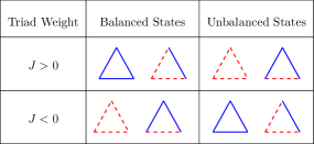
Our model investigates how the network will reach a balanced state as a result of the competition of triads with various weights in each temperature. We show that the temperature has a significant effect on the dynamics of the network. In the proposed model, the minimum of energy is different from $-1$ in structural balance theory and depends on the parameters of the probability distribution of weights ($\mu,\sigma$). The network experiences a balanced state based on the distinct concept of balance in positive and negative weighted triads. Inspired by the exponential random graph, using the Boltzmann distribution gives us the probability of selecting a specific graph configuration at a certain temperature within the set of graphs. The Boltzmann probability in canonical ensemble is, $\mathcal{P}(G)\propto e^{-\beta\mathcal{H}(G)}$, where $\beta=1/T$.

III Analysis

III.1 Mean-field solution

Considering a fully connected network, we study the weighted structural balance Hamiltonian Eq. (2) and present a solution for the model based on the mean-field approach which is exact in the limit of large system size. Let rewrite our Hamiltonian as $\mathcal{H}=\mathcal{H^{\prime}}+\mathcal{H}_{ij}$, $\mathcal{H}_{ij}$ includes all terms in the Hamiltonian that contain $S_{ij}$,

$$\mathcal{H}_{ij}=-S_{ij}{\sum_{k\neq{i,j}}J_{ijk}S_{jk}S_{ki}},$$ (4)

and $\mathcal{H^{\prime}}$ is the rest of the Hamiltonian that relates to other links. The mean value $\langle S_{ij}\rangle$ of $S_{ij}$ can be calculated as

$$\langle{S_{ij}}\rangle =(1)\times P(S_{ij}=1)+(-1)\times P(S_{ij}=-1)$$ (5)

$$=\frac{1}{\mathcal{Z}}\sum_{\{S^{\prime}\}}e^{-\beta\mathcal{H}^{\prime}}\sum_{S_{ij}={\left\{\pm{1}\right\}}}S_{ij}e^{-\beta\mathcal{H}_{ij}}$$

$$=\frac{\sum_{\{S^{\prime}\}}e^{-\beta\mathcal{H}^{\prime}}\left[e^{-\beta\mathcal{H}_{ij}(S_{ij}=+1)}-e^{-\beta\mathcal{H}_{ij}(S_{ij}=-1)}\right]}{\sum_{\{S^{\prime}\}}e^{-\beta\mathcal{H}^{\prime}}\left[e^{-\beta\mathcal{H}_{ij}(S_{ij}=+1)}+e^{-\beta\mathcal{H}_{ij}(S_{ij}=-1)}\right]}$$

$$=\frac{\left\langle e^{-\beta\mathcal{H}_{ij}(S_{ij}=+1)}-e^{-\beta\mathcal{H}_{ij}(S_{ij}=-1)}\right\rangle_{\mathcal{Z^{\prime}}}}{\left\langle e^{-\beta\mathcal{H}_{ij}(S_{ij}=+1)}+e^{-\beta\mathcal{H}_{ij}(S_{ij}=-1)}\right\rangle_{\mathcal{Z^{\prime}}}},$$

where $\mathcal{Z}=\sum_{{}_{\left\{G\right\}}}\exp{(-\beta\mathcal{H}(G))}$ is the partition function and we define: $\mathcal{Z^{\prime}}=\sum_{{}_{\left\{S^{\prime}\right\}}}\exp{(-\beta\mathcal{H^{\prime}})}$. Here, $\langle\cdots\rangle_{\mathcal{Z^{\prime}}}$ indicates average within ensemble of networks over all links except $S_{ij}$. We can expand each of the exponential terms and applying the mean-field approximation term by term. Approximating all correlations of higher order by the correlation between single pairs of links results in, terms like $\langle{(S_{jk}S_{ki})^{m}}\rangle$ can be written as $\langle{S_{jk}S_{ki}}\rangle^{m}$ in the mean-field approximation. Following this approximation and naming $p\equiv\langle{S_{ij}}\rangle$, the mean value of links is

$$p=\tanh(\beta\langle{\sum_{k\neq{i,j}}J_{ijk}S_{jk}S_{ki}}\rangle),$$ (6)

we call the expression within the expectation symbol in Eq. (6) the effective field each link feels and name it as per link field, $Q$,

$$Q\equiv\langle\sum_{k\neq{i,j}}J_{ijk}S_{jk}S_{ki}\rangle.$$ (7)

By analogy to the steps mentioned above, we rewrite our Hamiltonian as $\mathcal{H}=\mathcal{H^{\prime}}+\mathcal{H}_{jk,ki}$

$$\mathcal{H}_{jk,ki} =-S_{jk}(\sum_{l\neq{i,j,k}}J_{jlk}S_{jl}S_{kl})-S_{ki}(\sum_{l\neq{i,j,k}}J_{kil}S_{kl}S_{il})$$ (8)

$$-J_{ijk}S_{ij}S_{jk}S_{ki},$$

we replace $\sum_{l\neq{i,j,k}}$ by $\sum_{l\neq{i,j}}$ in the mean-field approximation. By this estimation we are counting the specific two-star on nodes $i,j,k$ twice but in averaging over the all two-stars on a link, $N-2$, this outnumbering is ignorable. This approximation allows us a convenient use of $Q$ definition. Now, we set up an equation for calculating the mean value of two-stars $q\equiv\langle{S_{jk}S_{ki}}\rangle$,

$$\langle{S_{jk}S_{ki}}\rangle=\frac{\langle e^{-\beta\mathcal{H}_{jk,ki}(S_{jk},S_{ki}=1)}-e^{-\beta\mathcal{H}_{jk,ki}(S_{jk}=1,S_{ki}=-1)}-e^{-\beta\mathcal{H}_{jk,ki}(S_{jk}=-1,S_{ki}=1)}+e^{-\beta\mathcal{H}_{jk,ki}(S_{jk},S_{ki})=-1}\rangle_{\mathcal{Z^{\prime}}}}{\langle e^{-\beta\mathcal{H}_{jk,ki}(S_{jk},S_{ki}=1)}+e^{-\beta\mathcal{H}_{jk,ki}(S_{jk}=1,S_{ki}=-1)}+e^{-\beta\mathcal{H}_{jk,ki}(S_{jk}=-1,S_{ki}=1)}+e^{-\beta\mathcal{H}_{jk,ki}(S_{jk},S_{ki})=-1}\rangle_{\mathcal{Z^{\prime}}}},$$ (9)

the mean-field approximation yields the following relations for the mean value of links and two-stars according to $Q$,

$$p=\tanh(\beta Q),\qquad q(Q,J_{ijk},\beta)=\frac{e^{2\beta Q}-2\,e^{-2\beta J_{ijk}\tanh(\beta Q)}+e^{-2\beta Q}}{e^{2\beta Q}+2\,e^{-2\beta J_{ijk}\tanh(\beta Q)}+e^{-2\beta Q}}.$$ (10)

We can derive a self-consistent equation for $Q$. Let think of a network involves distinct groups of two-stars, each characterized by its number of members $N_{i}$ and weight $J_{i}$; then, we manage to write Eq. (7) in the following form

$$Q =\sum_{i}J_{i}\ q(Q,J_{ijk}=J_{i},\beta)=N_{1}J_{1}q_{1}+N_{2}J_{2}q_{2}+\cdots=(N-2)\sum_{i}P(J_{i})\ J_{i}\ q_{i},$$ (11)

where in the last line we have used $P(J_{i})$ the probability density of having two-stars with weight $J_{i}$. The factor $(N-2)$ indicates the total number of two-stars on a link and $q_{i}$ counts for the average of two-stars with weight $J_{i}$. From Eq. (10) we see the average of two-stars, $q$, depends on the weight of the corresponding triad, $J_{ijk}$.

In the simplest case, we assume that there are two groups of two-stars with the number of members $N_{1}$, $N_{2}$, and weights $J_{1}$, $J_{2}$ on each link. Hence, Eq. (11) is written as

$$Q =N_{1}J_{1}q_{1}+N_{2}J_{2}q_{2}$$ (12)

$$=(N-2)\left\{P(J_{1})J_{1}q_{1}+P(J_{2})J_{2}q_{2}\right\},$$

$q_{1},q_{2}$ indicate the average of two-stars with weights $J_{1},J_{2}$ respectively. Using Eq. (10) to derive the mean value of two-stars of each group

$$\begin{split}&q_{1}=\frac{e^{2\beta Q}-2e^{-2\beta J_{1}\tanh(\beta Q)}+e^{-2\beta Q}}{e^{2\beta Q}+2e^{-2\beta J_{1}\tanh(\beta Q)}+e^{-2\beta Q}},\\ &q_{2}=\frac{e^{2\beta Q}-2e^{-2\beta J_{2}\tanh(\beta Q)}+e^{-2\beta Q}}{e^{2\beta Q}+2e^{-2\beta J_{2}\tanh(\beta Q)}+e^{-2\beta Q}},\\ \end{split}$$ (13)

multiplying $q_{1}$ in $N_{1}J_{1}$ and $q_{2}$ in $N_{2}J_{2}$ and summing them up, will come by a self-consistent equation based on $Q$

$$Q=N_{1}J_{1}q_{1}+N_{2}J_{2}q_{2}\equiv f(Q;\;N_{1},N_{2},J_{1},J_{2},\beta),$$ (14)

Figure 2: Graphical analysis of Eq. (15) for $N=50$, $T_{c}\simeq 28$. For $T_{1}<T_{c}$ the equation has three fixed points which two of them are stable and one is unstable. For $T_{2}>T_{c}$ the equation has only one stable fixed point.

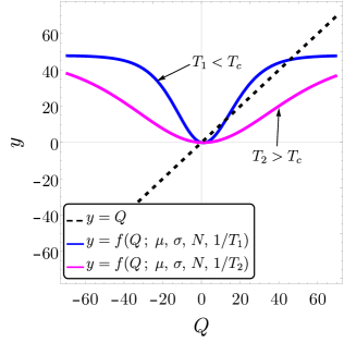
the intersection of the line $y=Q$ and the curve $y=f(Q;\;N_{1},N_{2},J_{1},J_{2},\beta)$ gives the solutions of Eq. (14).

Up to here, we succeed to derive a self-consistent equation by addressing Eq. (7) in discrete manner now let turn into continuous case by converting the summation to integral as

$$Q =(N-2)\int_{-\infty}^{\infty}J^{\prime}\ P(J^{\prime})\ q(Q,J^{\prime},\beta)\ dJ^{\prime}$$ (15)

$$=(N-2)\int_{-\infty}^{\infty}J^{\prime}P(J^{\prime})(\frac{e^{2\beta Q}-2e^{-2\beta J^{\prime}\tanh(\beta Q)}+e^{-2\beta Q}}{e^{2\beta Q}+2e^{-2\beta J^{\prime}\tanh(\beta Q)}+e^{-2\beta Q}})dJ^{\prime}$$

$$\equiv f(Q;\;\mu,\sigma,N,\beta),$$

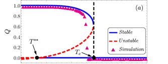
this is the continuous version of the self-consistent equation which we solve numerically. (Fig. 2) shows a plot of the forms $y=Q$ and $y=f(Q;\;\mu,\sigma,N,\beta)$ as a function of $Q$ for $N=50$, $\mu=1$, and $\sigma=0.1$ in two different temperatures. The intersection of line and curve gives the solutions of Eq. (15), which posses a first-order phase transition between states of high and low temperatures. For $T>T_{c}$ the system has only one stable fixed point $Q^{\star}=0$ which means each link feels a zero effective field. This is the consequence of the random distribution of two-stars of different signs and values on each link. For $T<T_{c}$ the system has three fixed points, the middle point is always unstable since the curve lies above $y=Q$ (the derivative of the $f(Q;\;\mu,\sigma,N,\beta)$ respect to $Q$ is bigger than one), the last point which stands for large $Q$ is always stable, and the zero point that switches from a stable (solid line) to an unstable (dashed line) fixed point in $T^{\star\star}$, Fig. 3(a).

The bifurcation diagram displays the kinds of possible solutions of Eq. (15) as a function of temperature [Fig. 3(a)]. We see that by approaching the critical point $T_{c}$ from above two other fixed points will be created as well as $Q^{\star}=0$. The critical temperature, $T_{c}$, indicates the phase transition of the system and the difference in the number of solutions of Eq. (15). $T^{\star\star}$ is the temperature that the zero switches from a stable to an unstable fixed point. The closeness of the stable and unstable line in $T^{\star\star}$ point causes disappearance of stable solutions for $T<T^{\star\star}$. The value of both temperatures $T_{c}$, $T^{\star\star}$ depend on the variance.

In the case of strong disorder (big variance), weights are so diverse and values can be far away from the mean value of probability distribution ($\mu=1$). Therefore, unlike the main idea of the mean-field method, the environment of triads is not homogeneous and each triad is experiencing different fields due to its surroundings. It means we do not expect the mean-field method to works well in this case. The remarkable effect of variance in the stability of the network will be addressed in the proceeding sections where we compare the simulation and analytical results. In the next section, we will see in detail that the variance is playing a crucial role in either achieving a reasonable analytical solution or its agreement with simulation. Finally, we calculate the mean value of triads, $r\equiv\langle S_{ij}S_{jk}S_{ki}\rangle$, by considering the mean-field approximation (see the Appendix)

$$r(Q,J_{ijk},\beta)=$$ (16)

$$\frac{e^{3\beta Q+\beta J_{ijk}}-3e^{\beta Q-\beta J_{ijk}}+3e^{-\beta Q+\beta J_{ijk}}-e^{-3\beta Q-\beta J_{ijk}}}{e^{3\beta Q+\beta J_{ijk}}+3e^{\beta Q-\beta J_{ijk}}+3e^{-\beta Q+\beta J_{ijk}}+e^{-3\beta Q-\beta J_{ijk}}}.$$

Based on the Hamiltonian Eq. (2) the energy is the mean value of weighted triads, $E=-\langle\sum_{i>j>k}J_{ijk}S_{ij}S_{jk}S_{ki}\rangle$, which can be written in the form of

$$E=-\sum_{i}P(J_{i})\ J_{i}\ r(Q,J_{ijk}=J_{i},\beta),$$ (17)

where $P(J_{i})$ is the probability density of finding a triad with weight $J_{i}$ and $r_{i}$ is the average of triads of weight $J_{i}$. Again considering continuous case energy equation can be written in the following form:

$$E=-\int_{-\infty}^{\infty}J^{\prime}\ P(J^{\prime})\ r(Q,J^{\prime},\beta)\ dJ^{\prime},$$ (18)

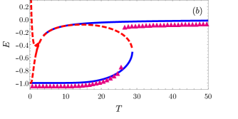
[Fig. 3.(b)] pictures the analytical solution of energy for $\sigma=0.1$ and its simulation result. There is a reasonable agreement between simulation and analytical solutions.

Figure 3: (a) Bifurcation diagram shows whether the normalized solutions of Eq. (15), $Q^{\star}$, are stable or not. The diagram displays $T^{\star\star}$, the temperature that the zero changes from a stable to an unstable fixed point, and $T_{c}$, the critical temperature that indicates the phase transition of the system. The simulation result is also shown to confirm the accuracy of our analytical solution. (b) Bifurcation diagram of Eq. (18) with normalized values and its corresponding simulation result.

III.2 Simulations

We start with a fully connected network. A link between two nodes $i$ and $j$ has the values of $+1$ or $-1$ corresponds to friendly or enmity relationship, respectively. We simulate a system with 50 nodes, $\mu=1$ and two different values of variance $0.1$, $10$. We thermalize our system with a given temperature by the Monte Carlo method. We are using the Metropolis algorithm; in each iteration, for a given temperature a link is selected randomly, and based on our Hamiltonian we calculate the energy difference $\Delta E=E_{2}-E_{1}$ if the energy of configuration after flip $E_{2}$ is less than prior $E_{1}$ ($\Delta E<0$), the selected link is flipped otherwise flip will be accepted with a probability equal to “exp$(-\beta\Delta E)$" where “$\beta$" is equal to the inverse of the temperature. Since we consider triads with different weights, it matters from which triad the random link is. Flipping a link that belongs to a big weighted triad will change the energy of the system significantly. Here, the role of the variance would appear. In weak disorder a large percentage of weights are around the mean value of probability distribution ($\mu=1$), so triads have equal weights approximately, whereas in strong disorder regime, weights are diverse and competition between triads of various weights prevents the network to reach a balanced state.

III.2.1 Weak disorder

In the case of small variance, $\sigma=0.1$, the majority of weights are positive (mean of probability was set to be in positive values $\mu=1$). In high temperatures, fluctuations are high and the total energy of the system is zero. As temperature decreases the links switch and triads change into balance whether they are positively or negatively weighted. Thermal fluctuation can overcome small weighted triads and flip links to satisfy energy minimization. Although triads of different weights compete with each other to determine the network destination, positive triads overcome the contest since they are the majority in terms of numbers and the balanced state of the network occurs as triads are in balanced configurations in the definition of $J>0$. The same will happen if the mean of probability was set to be in negative e.g, $\mu=-1$, with the difference that negative triads win the competition and a balanced state occurs in the definition of $J<0$.

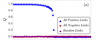
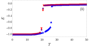
Figure. 4(a) displays the effective field each link feels respect to the temperature. The balanced final state of the system depends on the initial condition. In the case of all positive links, the final state is heaven so the normalized effective field in low temperatures is equal to one. For other initial conditions, the final state is bipolar and each link feels approximately equal pressure from positive and negative fields so the normalized effective field equals zero. Figure. 4(b) shows the energy simulation results versus temperature for different initial states (all links positive, all links negative, random links). The transition between balanced and random states happens in two different temperatures for all positive initial condition and two other conditions. Starting simulation with an all links positive network and decreasing the temperature, the system reaches to the balanced state at higher temperature. We see that the minimum energy of the network occurs in the mean value of the probability distribution which is in agreement with our expectation since the network mostly consists of triads with weights around $\mu=1$. Increasing the variance will increase the ratio of triads of variously weighted. We will address the big variances in the proceeding section.

Figure 4: (a) The effective field (the mean value of weighted two-stars), $Q$, vs. temperature. In high temperatures, each link feels a zero field because we have equal number of positive and negative two-stars. The final state of positive initial condition in low temperature is heaven so, $Q=1$. For other initial conditions, the final state is bipolar and an equal ratio of positive and negative effective field results in $Q=0$. (b) The energy of network vs. temperature for different initial states. In high temperature energy is zero since the system is in the random state and by decreasing temperature system is led to the balanced state.

III.2.2 Strong disorder

For strong disorder, the number of triads of different weights (positive and negative) are comparable to each other, e.g., for $\sigma>4$ the percentage of negative triads is more than $40$ therefore, there is a competition between negatively weighted triads and positive ones. There is no end to this competition even if we increase Monte-Carlo steps by order of magnitude; hence, we see that the system does not reach the global minimum at low temperatures. Generating random weights from a Gaussian distribution with a big variance will result in values that are not necessarily around the mean. Here, the diversity of weights and the comparable number of positive and negative triads cause the network to be unable to reach a balanced state. Notice we do not have such a situation in the weak disorder case since almost all triads have roughly equal weights.

Figure 5: (a) The effective field, Q, vs. temperature. In high temperatures, each link feels a zero field due to the random distribution of two-stars. Because of the diversity of weights in big variance, the behavior of this quantity deviates from the weak disorder case in low temperatures. (b) The energy of the network vs. temperature. The interaction between triads with various weights causes zero energy in high temperatures. In low temperatures, the existence of unbalanced triads causes energy increases so, the system does not reach a balanced state .

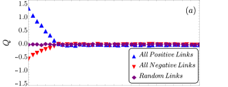
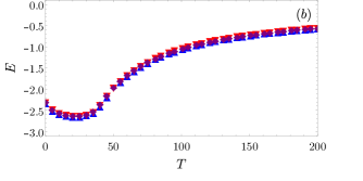
Figure. 5(a) displays the effective field each link feels, depends on the initial condition. The simulation for strong disorder shows in high temperature, $T\gg T_{c}$, the random distribution of positive and negative two-stars results in zero effective field on each link and in $T\ll T_{c}$, the existence of disorder in the network results in a deviation in the behavior of effective field from the weak disorder regime, Fig. 4(a). Beginning with the positive initial condition, in small disorder case the network reaches the heaven state and all triads are of the kind $\{+,+,+\}$, likewise, in big variance case, it is more probable to have balanced triads of a kind $\{+,+,+\}$, $\{-,-,-\}$ for $J>0$ and $J<0$ respectively so the number of positive two-stars overcomes. For the case of the negative initial condition, in the small disorder case, the network has an equal number of positive and negative two-stars since it achieves bipolar state and the balanced triads of kind $\{-,-,+\}$, similarly in strong disorder case the balanced triads are more probable to be of a kind $\{-,-,+\}$, $\{+,+,-\}$ for $J>0$ and $J<0$ respectively. In these mentioned kinds of triads two-stars are averagely negative so we see a negative value of $Q$ in $T\ll T_{c}$. Fig. 5(b) indicates the dynamics of the network with respect to the temperature for $\sigma=10$. It shows, all initial states diagrams overlay, in contrast with the small variance that positive initial state is isolated from two others Fig. 4(b). Our horizon toward the system’s evolution in the strong disorder regime will be opened by Fig. 6.

Figure 6: A sample unbalanced triad, $E_{ijk}=39$, is depicted. Each link shares in several triads (here, we have shown only three of them). The total energy of triangles on each link is shown, e.g., $E_{ij}$ is the sum of the energy of triangles on the link $i,j$. The negative value of energy on each link shows that the majority of triads were balanced.

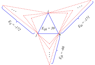
It represents, the only possible situation that the unbalanced triads can survive in the network is to be surrounded by a large number of balanced ones. The general strategy is to update the links in each temperature. If switching a link results in by a negative energy difference $\Delta E<0$, then the flip will be accepted; otherwise, the condition of a link to be flipped is measured by Boltzmann probability $p\propto$ exp$(-\Delta E/T)$ and the temperature gives a chance for the links to be flipped. Investigating the structure of the network in three regimes of temperature yields:

(i) $T\ll T_{c}$, it is more probable that the system getting stuck on the local minimum and links do not have the chance of flip, hence, the system can not escape from the local minimum and unbalanced triads froze in their states. In the Fig. 6, we chose a sample unbalanced triad and calculated the sum of the energy of triads on each edge. The flipping of each link results in a growth in energy $(\Delta E>0)$ and the Boltzmann probability of flipping is about to zero $p\cong 0$ so unbalanced triads would not change. Then the network has more unbalanced triads in these temperatures and we see that the energy increases.

(ii) $T\simeq T_{c}\simeq 28$, with increasing temperature, links have the chance of flipping due to the Boltzmann probability and some of the unbalanced triads change into balanced. The energy minimum occurs in temperatures around $20-30$ where the number of unbalanced triads is the least with respect to the other temperatures.

(iii) $T\gg T_{c}$, when temperature tends to infinity, based on the Boltzmann probability, links have the chance of flipping even if the energy increases. The temperature provides the possibility that unbalanced triads exist in the network. Therefore, the network is a combination of balanced and unbalanced triads which results in zero energy.

From another point of view, the diagram of the energy versus temperature in the strong disorder regime, [Fig. 5(b)] shows, in the case of big variance, energy increases at low temperature, although we expect to see the reduction in the number of unbalanced triads and the minimization of energy as temperature decreases. This figure is schematically similar to the resistivity versus temperature diagram in the Kondo effect, kondo1 ; kondo2 ; we expect to see low resistivity in low temperatures, but the existence of impurity in the lattice which disturbs the periodic layout of the lattice results in an unusual behavior of some metals. We emphasize that we have no claim on the Kondo effect concept in this study; merely there is a similar behavior between these two phenomena. As we mentioned above the mean-field approximation does not work well in this regime due to heterogeneity of weights. Here the difference between our proposed model and structural balance theory emerges. We see the energy will reach zero in temperatures of the order $10^{4}$.

IV CONCLUSIONS

Here, we proposed a model that takes into account weights in the structural balance theory. Results show that it is not a simple modification to unweighted balance theory and our analysis demonstrates the importance of variance in achieving a balanced state. We studied the model theoretically through the mean-field method that suites perfectly the Monte Carlo simulation results in the weak disorder regime. Looking at the dynamics of the system in a completely connected network under two regimes revealed that the system posses a first-order phase transition because of a discontinuous jump in the energy of the system. Since increasing the variance corresponds to the increase in the number of negative triads or more disorder in the network, then it takes longer steps for the system to reaches a balanced state in low temperatures in contrast to small variances hence, the critical temperature depends on the variance. In the process of the evolution, although each kind of triads whether positive or negative wants to make the network balanced in its definition, we see the unbalanced triads still persist in low temperatures in strong disorder, unlike weak disorder and balance theory. This result represents a pseudo-Kondo effect behavior in the energy changes versus temperature which states the remarkable difference between our model and balance theory. Our proposed model goes beyond the equally weighted triads and pays attention to differences of relations so it can serve as a practical tool in dealing with real weighted networks.

Appendix A Calculation of The Mean Values Triads

In this part, we want to calculate the mean value of triads. We write the Hamiltonian as $H=H^{\prime}+H_{\Delta}$, where $H_{\Delta}$

$$H_{\Delta} =-S_{ij}(\sum_{l\neq{i,j,k}}J_{ijl}S_{il}S_{lj})-S_{jk}(\sum_{l\neq{i,j,k}}J_{jkl}S_{kl}S_{lj})$$ (19)

$$-S_{ki}(\sum_{l\neq{i,j,k}}J_{ikl}S_{il}S_{lk})-J_{ijk}S_{ij}S_{jk}S_{ki},$$

consist of terms dedicates to each link $S_{ij}$ , $S_{jk}$ and $S_{ki}$ individually and the last term denotes a triad of all those. We have

$$\langle{S_{ij}S_{jk}S_{ki}}\rangle=\sum_{\{S_{ij},S_{jk},S_{ki}\pm 1\}}P(S_{ij},S_{jk},S_{ki})S_{ij}S_{jk}S_{ki}.\\$$ (20)

Keep all the calculations similar to what has been done for two-stars, again in the mean-field approximation we estimate each of three inequality summations by two inequality, for convenient use of $Q$ definition. Considering all possible configurations of triplet $S_{ij}S_{jk}S_{ki}$, there will be eight different forms, where $H^{abc}_{\Delta}\equiv\ H_{\Delta}(S_{ij}=a,S_{jk}=b,S_{ki}=c)$, and we write it as

$$-\beta H^{+++}_{\Delta} =3\beta Q+\beta J_{ijk},$$ (21)

$$-\beta H^{---}_{\Delta} =-3\beta Q-\beta J_{ijk},$$

$$-\beta H^{++-}_{\Delta} =\beta Q-\beta J_{ijk},$$

$$-\beta H^{+-+}_{\Delta} =\beta Q-\beta J_{ijk},$$

$$-\beta H^{-++}_{\Delta} =\beta Q-\beta J_{ijk},$$

$$-\beta H^{--+}_{\Delta} =-\beta Q+\beta J_{ijk},$$

$$-\beta H^{-+-}_{\Delta} =-\beta Q+\beta J_{ijk},$$

$$-\beta H^{+--}_{\Delta} =-\beta Q+\beta J_{ijk},$$

$$r(Q,J_{ijk},\beta)=\frac{e^{3\beta Q+\beta J_{ijk}}-3e^{\beta Q-\beta J_{ijk}}+3e^{-\beta Q+\beta J_{ijk}}-e^{-3\beta Q-\beta J_{ijk}}}{e^{3\beta Q+\beta J_{ijk}}+3e^{\beta Q-\beta J_{ijk}}+3e^{-\beta Q+\beta J_{ijk}}+e^{-3\beta Q-\beta J_{ijk}}}.$$ (22)

References

- (1) F. Heider, J. Psychol., 21, 107 (1946).
- (2) F. Heider, The Psychology of Interpersonal Relations, Wiley, New York, 1958.
- (3) D. Cartwright , & F. Harary, Psychol. Rev., 63, 277, (1956).
- (4) S. Wasserman and K.Faust, Social Network Analysis: Methods and Applications , Cambridge University Press, 1994.
- (5) James A. Davis, Hum. Relat., 20, 181, (1967).
- (6) Robert K. Leik, B. F. Meeker, Mathematical sociology, Prentice-Hall Englewood Cliffs, N.J, 1975
- (7) H. Saiz, J. Gómez-Gardeñes, P. Nuche, A. Girón, Y. Pueyo, and C. L. Alados, Ecography 40, 733, (2017).
- (8) J. Hart, J. Peace Res., 11, 229, (1974).
- (9) S. Galam, Physica A, 230, 174, (1996).
- (10) A. Bramson, K. Hoefman, M. van den Heuvel, B. Vandermarliere, and K. Schoors, Measuring Propagation with Temporal Webs, N. Masuda, P. Holme, Springer, Singapore, (2017).
- (11) P. Singh, S. Sreenivasan, B. K. Szymanski, & G. Korniss, Phys. Rev. E, 93, 042306, (2016).
- (12) C. Altafini, PloS one 7, e38135, (2012).
- (13) F. Oloomi, R. Masoumi, K. K. Pour, A. Hosseiny, G. R. Jafari, Phys. Rev. E 103, 022307, (2021).
- (14) A. Kargaran, M. Ebrahimi, M. Riazi, A. Hosseiny, and G. R. Jafari, Phys. Rev. E 102, 012310, (2020).
- (15) S. Sheykhali, A. H. Darooneh, G. R. Jafari, Physica A, 123882, (2019)
- (16) L. Hedayatifar, F. Hassanibesheli, A. Shirazi, S. V. Farahani, and G. R. Jafari, Physica A 483, 109, (2017).
- (17) F. Hassanibesheli, L. Hedayatifar, H. Safdari, M. Ausloos, and G. R. Jafari, Entropy, 19, 246, (2017).
- (18) M. Saeedian, N. Azimi-Tafreshi, G. R. Jafari, and J. Kertesz, Phys. Rev. E, 95, 022314, (2017).
- (19) F. Rabbani, Amir H. Shirazi, and G. R. Jafari, Phys. Rev. E, 99, 062302, (2019).
- (20) R. Masoumi, F. Oloomi, A. Kargaran, A. Hosseiny, GR Jafari, arXiv preprint arXiv:2008.00537
- (21) A. M. Belaza, K. Hoefman, J. Ryckebusch, A. Bramson, M. van den Heuvel, and K.Schoors, PLoS ONE, 12, (2017).
- (22) A. M. Belaza, J. Ryckebusch, A. Bramson, C. Casert, K. Hoefman, K. Schoors, M. van den Heuvel, and B. Vandermarliere, Physica A, 518, (2019).
- (23) T. Antal, P. L. Krapivsky, & S. Redner, Phys. Rev. E 72, 036121, (2005).
- (24) T. Antal, P. L. Krapivsky, & S. Redner, Physica D 224, 130, (2006).
- (25) K. Kułakowski, P. Gawroński, and P. Gronek, Int. J. Mod. Phys. C 16, 707, (2005).
- (26) S. A. Marvel, S. H. Strogatz, and J. M. Kleinberg, Phys. Rev. Lett. 103, 198701, (2009).
- (27) S. A. Marvel, J. Kleinberg, R. D. Kleinberg, and S. H. Strogatz, Proc. Natl. Acad. Sci. USA, 108 (5) 1771 (2011).
- (28) J. Leskovec, D. Huttenlocher, and J. Kleinberg, Conference on Human Factors in Computing Systems (Association for Computing Machinery, New York, 2010).
- (29) A. Kirkley, G. T. Cantwell, and M. E. J. Newman Phys. Rev. E, 99, 012320, (2019).
- (30) G. Facchetti, G. Iacono, and C. Altafini, Proc. Natl. Acad. Sci. USA 108, 20953 (2011).
- (31) E. Estrada and M. Benzi, Phys. Rev. E, 90, 042802, (2014).
- (32) E. Estrada, Discrete. Appl. Math, 268, (2019).
- (33) M. E. J. Newman, Phys. Rev. E 70, 056131, (2004).
- (34) M. E. J. Newman, Phys.Rev. E 64, 016132, (2001).
- (35) S. H. Yook, H. Jeong, A.-L. Barab´asi, and Y. Tu, Phys. Rev. Lett. 86, 5835, (2001).
- (36) J. D. Noh and H. Rieger, Phys. Rev. E 66, 066127, (2002).
- (37) A. Barrat, M. Barthelemy, R. Pastor-Satorras, and A. Vespignani, Proc. Natl. Acad. Sci. USA 101, 3747–3752, (2004).
- (38) A. Barrat, M. Barthelemy, and A. Vespignani, Phys. Rev. Lett. 92, 228701, (2004).
- (39) B. Tadic, M. Suvakov, M. Andjelković, and G. J. Rodgers, Phys. Rev. E 102, 032307, (2020).
- (40) B. Tadic, N. Gupte, arXiv preprint arXiv:2012.07506
- (41) A Karimi Rizi, M. Zamani, Amir H. Shirazi, G. R. Jafari, János Kertész, Frontiers in Physiology,11, 1792,(2021).
- (42) Z. Moradimanesh, R. Khosrowabadi, M. Eshaghi Gordji,G. R. Jafari , Sci. Rep.,11, 1966, (2021).
- (43) P. W. Holland and S. Leinhardt, J. Am. Stat. Assoc.. Am. Stat. Assoc., 76, 33, (1981).
- (44) J. Besag, JRSS B,36, 192, (1974).
- (45) O. Frank and D. Strauss, J. Am. Stat. Assoc. 81, 832, (1986).
- (46) D. Strauss, SIAM Rev., 28, 513, (1986).
- (47) S. Wasserman and P. Pattison, Psychometrika 61, 401, (1996).
- (48) C. J. Anderson, S. Wasserman, and B. Crouch, Soc. Netw. 21, 37, (1999).
- (49) T. A. B. Snijders, P. E. Pattison, G. L. Robins, and M. S. Handcock, Sociol. Methodol. 36, 99, (2006).
- (50) G. Robins, P. Pattison, Y. Kalish, and D. Lusher, Soc. Netw. 29, 173, (2007).,
- (51) S. J. Cranmer and B. A. Desmarais, Political Anal., 19, 6686, (2011).
- (52) T. A. B. Snijders, Annu. Rev. Sociol. 37, 131, (2011).
- (53) J. Park and M. E. J. Newman, Phys. Rev. E 70, 066146, (2004).
- (54) J. Park and M. E. J. Newman, Phys. Rev. E 70, 066117, (2004).
- (55) J. Park and M. E. J. Newman, Phys. Rev. E 72, 026136, (2005).
- (56) J. Kondo, Progress of Theoretical Physics 32, 37, (1964).
- (57) A. C. Hewson, J. Kondo, Scholarpedia 4, 7529, (2009).