Learning 3D Dynamic Scene Representations
for Robot Manipulation
Abstract
3D scene representation for robot manipulation should capture three key object properties: permanency – objects that become occluded over time continue to exist; amodal completeness – objects have 3D occupancy, even if only partial observations are available; spatiotemporal continuity – the movement of each object is continuous over space and time. In this paper, we introduce 3D Dynamic Scene Representation (DSR), a 3D volumetric scene representation that simultaneously discovers, tracks, reconstructs objects, and predicts their dynamics while capturing all three properties. We further propose DSR-Net, which learns to aggregate visual observations over multiple interactions to gradually build and refine DSR. Our model achieves state-of-the-art performance in modeling 3D scene dynamics with DSR on both simulated and real data. Combined with model predictive control, DSR-Net enables accurate planning in downstream robotic manipulation tasks such as planar pushing. Code and data are available at dsr-net.cs.columbia.edu.
Keywords: Predictive Model, Manipulation, 3D Vision
1 Introduction
Our physical world is three-dimensional, where the full extent of objects – their shape and motion – exists and persists in 3D space. Despite this, the vast majority of visual predictive models currently used in robotics, which predict the motion of objects under the effect of an applied action, remain limited to only predicting 2D motion (i.e. optical flow) of partial observations, e.g. predicting the 2D flow of pixels [1, 2], or predicting the 3D scene flow of visible points from a partial point cloud [3, 4]. Unfortunately, modeling the motion of only visible surfaces often leads to data degeneration, where objects fade and vanish from the representation as they become occluded. This causes the predictive models to perform poorly in cluttered environments, in which objects frequently appear, disappear, then reappear in view as the robot move them around.
In this work, we investigate the benefits of learning a complete and persistent 3D scene representation for visual predictive modeling. We present 3D Dynamic Scene Representation (DSR): a 3D volumetric scene representation that simultaneously discovers, tracks and reconstructs novel objects and predicts their motion under a robot’s interactions. Specifically, the representation captures three object properties, all of which have long been argued as crucial to human scene understanding [5].
-
•
Permanence: visual information is aggregated into a persistent 3D representation. This means that as objects disappear from view due to occlusion, they remain in the representation. This enables more accurate predictions of object motion when it is moved by other objects in occlusion, or when it gradually reappears in view.
-
•
Amodal completeness: from partial observations of the scene, DSR infers complete 3D occupancy of each object, including regions that are not directly observed. This attribute enables it to predict the rigid body motion of the entire object instead of only visible surfaces.
-
•
Spatiotemporal continuity: the representation recognizes individual object instances and tracks their identity over time.
-
•
Interpretability: DSR explicitly models object instances, geometry, and motion, makes it easy to be used out-of-the-box for high-level reasoning in robotic applications.
To learn this scene representation, we present DSR-Net, a 3D recurrent neural network that consists of two major components: 1) a scene encoder that encodes visual observations (i.e., depth images) into a volumetric 3D scene representation, and 2) a motion prediction network that takes in the 3D scene representation and an action to be performed by the robot and predicts volumetric scene flow. The scene flow is then used to spatially warp the current scene representation before combining it with the 3D scene representation of the next time step. The warping operation allows the network to aggregate information over time in a spatially coherent way. DSR-Net is trained end-to-end in simulation and then tested in the real world with a robotic manipulator on a tabletop setup. Our experiment result shows that our system achieves state-of-the-art performance in predicting the rigid body motion of novel objects under robot interaction in unstructured cluttered environments.
The contributions of our paper are three-fold. First, we introduce a new 3D dynamic scene representation (DSR) that captures object permanence, amodal completeness, and continuity – desirable properties as part of a perception stack for downstream robot manipulation tasks. Second, we propose DSR-Net, an end-to-end framework that learns such 3D representations via 3D convolutions. Third, we build a new benchmark dataset with over 80,000 simulated interactions and 1,500 real-world interactions for learning and evaluating dynamic 3D scene representations. Our experiments in both simulation and in the real-world show that DSR-Net achieves state-of-the-art performance in predicting 3D scene dynamics. Furthermore, it enables more accurate action planning in manipulation tasks such as planar pushing. Please find additional result and videos in supplementary material.

2 Related work
Learning scene (or state) representations from visual data is a long-standing task in vision and robotics. Many different scene representations have been proposed for different environments, types of interaction, and applications. Our method learns an 3D scene representation for dynamic, multi-object environments under robot interactions. Here we summarize most relevant works.
Passive perception.
Most traditional computer vision tasks such as object detection or segmentation can be considered as extracting a high-level scene representation from passive observation, such as a single RGB image. However, these 2D representations cannot be directly applied in robotic applications that need to be operated in 3D. Recently many works have studied the problem of inferring 3D scene representations from partial observations such as a single color image [6, 7] or a depth map [8, 9]. These representations are explicit, often in the form of 3D volumes or polygonal meshes. Latest papers in the field have also explored integrating neural nets for learning implicit 3D representations for objects and scenes [10, 11, 12, 13]. While these scene representations have been used for robotics applications such as object grasping [14, 15], they handle static environments only and cannot be directly applied in dynamic scenes.
Active perception.
Systems that may update the camera viewpoint for exploration and representation building are often referred to as active perception systems [16, 17]. Cheng and Katerina [18] proposed an active vision system that actively selects new camera viewpoints for estimating 3D object geometry and recognizing their identities. The representation learned by this system has been used for reinforcement learning [19]. There are also models that actively learn a 3D scene representation from multi-view images or videos for better 3D geometry [20, 21], shape correspondences [22, 23, 24], motion [25, 26], semantic category [27, 28], or multiple objectives [1]. While active perception systems may collect additional information about object geometry with a moving camera, they still focus on static scenes, where there is no signal about object dynamics or physics. In contrast, our model observes a robot’s active interactions with objects in the scene (e.g., pushing). As a result, the scene representation can model and predict object dynamics under interaction, which is critical for task and action planning.
Interactive perception.
Interactive perception is about perception facilitated by interaction with the environment [29]. An important topic in interactive perception is on learning predictive and dynamic scene representations that are conditioned on current observations and interaction for manipulation[30, 31]. Recently, a few visual predictive models have been proposed to learn an object-centric representation [32, 33, 34], as well as to model 3D motion for rigid shapes [3, 4]. However, all these works predict motion in the form of per-pixel flow, which only considers the partial, observable surface, and does not leverage past interactions and observations. Therefore, the scene representations produced by these methods are often incomplete and inaccurate. The model that is most relevant to ours is DensePhysNet [35], which learns to aggregate multiple interactions for a dense, 2D scene representation. However, it fails to model 3D relations, such as occlusion, and thus cannot provide a scene representation that maintains object permanence when there are occlusions.
3 Dynamic Scene Representation Network (DSR-Net)
In this section, we first provide an overview of DSR-Net’s network design and its advantages, then we provide description on each module and how to use it in robot manipulation. Fig. 2 shows an overview of DSR-Net. At each step, the scene encoder outputs a 3D scene representation that aggregates the new observation (i.e., depth) with the past scene representation . is then used to predict amodal object instance mask . In parallel, the motion predictor infers the object motion given the robot’s action and current scene representation. The predicted motion and object instance mask are combined to compute voxel-level scene flow . Finally, the scene flow is used to warp the scene representation to obtain that is aligned with observation in the next interaction step and used for history aggregation.
Our DSR-Net design provides four advantages compared to existing visual predictive models. First, by using a 3D volumetric representation, DSR-Net naturally models objects’ amodal 3D shape, regardless of occlusion. Second, by warping the previous scene representation using the predicted motion before concatenating it with the new observation, the network manages to aggregate history information in a spatially coherent manner: the same voxel stores information of the same object from past and new observations, regardless of their motion. Third, by leveraging history information the representation is able to capture object permanence and continuity. Finally, all these properties allow the network to predict more accurate object motion and be useful for manipulation tasks.

Scene encoder (Fig. 2a):
Each depth observation is encoded with a truncated signed distance function (TSDF) with voxel size 0.004m. The scene encoder concatenates the current observation (12812848 TSDF volume) and the warped representation from last step (the history aggregation part will includes more details). Twenty-two 3D convolution layers are applied to generate an output scene representation with a size of 812812848.
Action encoder (Fig. 2b):
In our setup, robots interact with the scene via pushing. The action can be discretized and represented by a tuple of integers , where are the start coordinates of the push in Cartesian space, and represents one of pre-defined directions of a push. Inspired by prior work [36], we use the action map for input form in order to provide spatial alignment with scene representation. An action is represented as a one-hot matrix with a size of 8128128, where is and other places are filled with . The action encoder encodes the action as two embeddings with size of 163232 and 86464.
Motion prediction (Fig. 2c):
The motion prediction network estimates transformations for every object based on the aggregated scene representation and action applied to the scene. The motion decoder predicts transforms, one for each of the predicted masks. We fix the last transformation () as an identical transformation since the background is static. A transform describes a rigid body transform , specified by a rotation and a translation . Under this transformation, 3D point moves to . We represent rotations using a Euler transform vector. Given the predicted transforms and masks, the transform layer produces a blended point cloud from the input points: , where is the 3D output point corresponding to voxel . Then the predicted scene flow of voxel is . The motion loss is Mean Square Error (MSE) between the predicted scene flow and ground truth.
Amodal instance mask prediction (Fig. 2d):
The mask predictor outputs a voxel-wise probability distribution over the classes. Following the standard practice as in prior works [3, 37], we use as the maximum number of objects to be handled in our experiment. As shown in supplementary material, the trained model is able to generalize to test cases with fewer objects than the maximum number of objects. During training, we need a specific order to calculate the loss for mask prediction and encourage temporal consistency over time. At each step, we enumerate all the permutations and select the optimal matching and it serves as ground truth for the next step. Specifically, in the first step, its optimal matching is also used as ground truth for training right now. Concretely, given the mask prediction and ground truth for each category, we calculate the negative log-likelihood loss: . The loss of a matching is the summation of each category. The optimal matching means it has the smallest matching loss: Once we find the correct order for the ground truth, the loss between predicted mask and ground truth is computed with Cross Entropy loss.
Forward warping for spatially aligned history aggregation:
To aggregate history, we warp the scene representation with the predicted scene flow and mask prediction to produce features that are spatially aligned across multiple steps. Here we use trilinear interpolation for 3D warping because truncation or direct nearest neighbor wrapping results in more empty holes when several voxels are moving to the same position. Let be the coordinates of voxel in the input representation, be the coordinates of a voxel in the warped representation, and is the predicted scene flow of . The weight contribution of to is computed by:
where is the predicted probability that belongs to any object. The last channel (d=k-1) always represents empty space. Let represent the input feature value at , then output the feature at after warping is computed as: .
Loss function.
The final loss function is , where is the Error of motion prediction and is the loss of mask prediction and is a weighting factor.
3.1 Applying DSR in Robot Manipulation
We now demonstrate how DSR can be used in manipulation. Specifically, the goal of the task is to control a robot arm to push objects in the scene to match a target state. With our learned model, we perform temporally extended planning by choosing a sequence of actions that can be executed in the environment. Among different planning approaches, we choose model-predictive control (MPC) to take advantage of our predictive model.
We apply a simple shooting-based MPC method [38] to generate and plan for a sequence of actions that minimize the cost. First, we sample actions around predicted masks from our DSR model, since only these actions are close to the objects. This allows us to have a much smaller sample size of actions and make our decision making faster. Then, we compute the cost based on the next state predictions, which include the pivot points and masks in the next state. Specifically, we have , where are candidate actions, is the Mean Square Error between target and predicted positions (computed by predicted mask) of each object, is the IoU between the predicted mask and target state, is a weighting factor for each channel. Finally, we choose the sequence of actions that has the lowest cost.
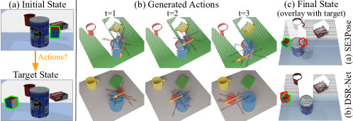
Since DSR maintains object permanence in the representation, it enables the planning algorithm to use the full state information including the occluded objects. For example, in Fig. 3, the robot has to push an occluded cube to a target location. This is impossible with SE3-Pose-Net – since it models only visible surfaces, the object is completely missing due to occlusion (t=3) and therefore a wrong action is selected. With DSR, the control policy is able to sample actions around the occluded object to predict the next state and cost accurately. Quantitative result are shown in Sec. 5.3.
4 Dynamic Scene Representation (DSR) Benchmark
To quantitatively evaluate predictive models, we need a dataset that contains robot interactions and ground object motion. Since there is no existing dataset containing this information (especially with real-world robot interactions), we construct a new dynamic scene representation (DSR) benchmark that contains both simulation and real-world data for training and evaluation.
Simulation data.
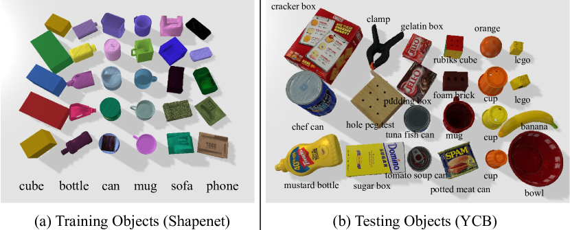
We use two types of objects in simulation training data: (1) cubes with different sizes m, and (2) 44 shapenet objects of 5 categories: mug (5), bottle (14), can (6), phone (10), and sofa (9). For each sequence, we choose 4 objects and randomly drop them on the workspace (m m). Then the robot executes 10 random pushing actions with a simple heuristic-base policy that encourages the change of spatial order and prevents moving objects out of the workspace. Details of the policy are described in the supplementary material. In total, there are 8,000 sequences with 80,000 interactions for training. We also generate a testing dataset using YCB objects [33] with the same interaction policy. This includes 400 sequences with 4,000 interactions.
Real-world data.
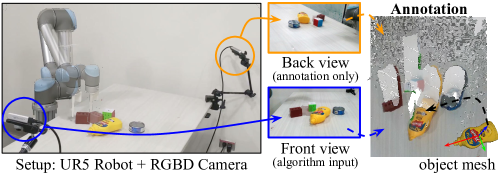
Our real-world setup consists of a UR5 robot with a cylinder pusher tool and two calibrated RGB-D cameras. Fig. 4 shows the setup and YCB objects [33] used in the real-world experiments. To accurately annotate the ground truth object pose under occlusion, we use an additional calibrated RGB-D camera in the setup to provide a backview of the workspace (Fig. 4 left and middle). We use the same discrete action space to collect real data. During annotation, we combine the 3D point clouds from both views to obtain a complete observation for the entire workspace. Fig. 4 right shows our annotation user interface. Users can control the object meshes’ 6DoF poses with keyboard to match the pose in the scene. In total, we collect 90 sequences with 900 interaction steps.
Train/Test split.
In simulation, all models are trained with 8,000 sequences with ShapeNet objects and tested on 400 sequences with novel YCB objects. The real-world dataset is split into 50 finetuning sequences and 100 testing sequences. In the following experiments, models labeled with “ft” are finetuned with the 50 sequences, all the other models are directly tested with realworld data without finetune. All qualitative result (except SE3 and SE3PoseNet) are using model without finetune.
5 Evaluation
We designed a series of experiments in both simulation and the real world using the benchmark data described in Sec. 4 to validate design decisions, and to compare with other models that predict future scene representations. Specifically, we want to see whether DSR-Net is able to
-
(1) Accurately predict object motion under different robot interactions;
-
(2) Aggregate the history and encodes object permanence and continuity; and
-
(3) Improve the performance of down-stream manipulation tasks.
| Simulation | Real | ||||
| visible | full | visible | full | ||
| 2D | 2DFlow ft [3] | 8.24 | - | 7.63 | - |
| SE3-Net ft [3] | 7.84 | - | 6.91 | - | |
| SE3Pose-Net ft [4] | 13.01 | - | 10.49 | - | |
| 3D | 3DFlow | 7.34 | 0.093 | 6.80 | 0.094 |
| SingleStep | 5.94 | 0.086 | 6.64 | 0.093 | |
| DSR-Net | 5.54 | 0.082 | 6.51 | 0.090 | |
| DSR-Net ft | - | - | 3.33 | 0.048 | |
5.1 Motion Prediction
First we want to evaluate the learned scene representation on predicting object motion under robots’ interaction. We use the Mean Squared Error (MSE) to evaluate the predicted 3D scene flow. For image based approaches, the MSE is computed and averaged for pixels of the visible surface, same as in SE3-Net [3]. For voxel-based approaches, the MSE is computed and averaged over the voxels on visible surfaces of the object (visible) and all voxels (full) separately.

Baselines:
In this experiment, we compare our algorithm with the following predictive models:
-
•
2DFlow [3]: it predicts per-pixel scene flow for the visible surface.
-
•
SE3-Net [3]: it predicts per-object masks and SE3 motions
-
•
SE3Pose-Net [4]: it predicts per-object poses, masks, and SE3 motions
-
•
3DFlow: it predicts per-voxel scene flow for the entire 3D volume.
-
•
SingleStep: DSR-Net without history aggregation.
Compared with state-of-the-art predictive models.
Tab. 1 shows quantitative comparisons of predicted motion. Since most voxels are static, the error of full volume is much smaller than the visible surface error. Fig. 5 shows qualitative comparisons among our model, SE3-Net, and SE3Pose-Net. The visualization suggests that the motion estimation in SE3-Net is limited to visible surface and cannot model occluded regions. In addition, the mask prediction in SE3-Net only handles the moving object, treating all other objects as background. This is because SE3-Net predicts masks based on both observation and action, where the network learns to first identify the moving objects and then predict mask and motion for these objects only. The mask prediction of SE3Pose-Net is independent from action; therefore, it has to predict masks for all objects in the scene. However, the motion prediction of SE3Pose-Net is based on object poses without considering their detailed geometry. This fact makes SE3Pose-Net perform worse in motion prediction. In contrast, our model produces 3D amodal masks for all objects in the scene and predicts the object motion more accurately.
5.2 Temporal Information Aggregation
| Simulation | Real | |||
|---|---|---|---|---|
| unordered | ordered | unordered | ordered | |
| GTWarp | 0.807 | 0.807 | 0.646 | 0.645 |
| SingleStep | 0.753 | 0.526 | 0.613 | 0.485 |
| NoWarp | 0.762 | 0.756 | 0.625 | 0.624 |
| DSR-Net | 0.772 | 0.767 | 0.628 | 0.628 |
In this section, we evaluate whether DSR-Net is able to effectively aggregate the history information to capture object permanence and continuity. We use two types of intersection over union (IoU) scores on 3D amodal instance masks as the evaluation metric: unordered and ordered IoU. To compute unordered IoU, we obtain the object order for each step by permuting the objects’ order and use the one that maximizes the average IoU over all objects as the ground truth order. The order of step is calculated by , where is the number of objects. For ordered IoU, we permute the object instance index once and use the order that best matches the entire sequence as the ground truth order: , where is the number of interactions. To achieve a high ordered IoU, the system needs to maintain a consistent order of object instance throughout the interaction steps. Therefore, this metric reflects the continuity of the scene representation over time. Besides, since the 3D IoU is evaluated on all the voxels in the scene regardless of occlusion, this metric also naturally measures the permanence of the scene representation under occlusion.
Baselines.
In this experiment,we compare our aggregation model with following alternatives:
-
•
SingleStep: it does not use any history aggregation.
-
•
NoWarp: it does not warp the representation before aggregation.
-
•
GTWarp: it warps the representation with ground truth motion (i.e., performance oracle).
Does history aggregation help in on amodal shape completion?
The unordered IoU in Tab. 2 measures the quality of 3D amodal shape completion without consider the objects’ identity. The result demonstrates that by effectively aggregate the past observations, our method is able to infer a more accurate scene representation in terms of modeling an object’s complete 3D geometry from partial observations (+1.6% improvement in unordered IoU compare to the single step model). In the following experiments, we will evaluate the object permanence and continuity using “ordered IoU”.
Does DSR encode object permanence?
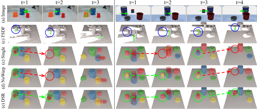
To evaluate the object permanence, we examine the network’s ability to infer an object’s existence during occlusion. Fig. 6 shows amodal mask estimation under occlusion in both real world and simulation cases. There are two static-occlusion cases (t=1-2 in the real and simulation example), where the occluded object is not moving, and one dynamic-occlusion case (t=3-4 in the simulation), where the moving object becomes occluded. The SingleStep model fails in both. The NoWarp model can handle one of static occlusion cases, since the history contains the information of the static object. However, it cannot handle dynamic occlusion due to the lack of historical motion. DSR-Net is able to handle both static and dynamic occlusions.
Does DSR encode object continuity?
A model that captures spatiotemporal continuity should maintain a consistent object identity overtime. We evaluate this and show the results in the ordered IoU in Tab. 2. Fig. 7 presents qualitative results of mask prediction after several interactions. Unlike the SingleStep model, which is sensitive to the spatial order, our model maintains spatiotemporal continuity via consistent labeling of object instances. In the simulation demonstration, DSR-Net can even track visually indistinguishable objects, whose positions are swapped after several interactions. It proves that the continuity owes to history aggregation, instead of visual appearance. Note that this happens to align with classical findings in developmental psychology [5]. The small gap between unordered and ordered IoUs in Tab. 2 demonstrates that our DSR-Net achieves a consistent order of object instances during an interaction sequence; SingleStep has a much bigger gap, indicating that it fails to track object identity without history aggregation.

Does motion prediction help in history aggregation?
To test the effect of motion prediction on history aggregation, we compare our model with NoWarp. The plot in Tab. 2 shows that, with spatial-aligned features, the algorithm produces a more accurate scene representation. In both simulation and real-world test sets, DSR-Net consistently achieves higher order and unordered IoUs. Further, if we warp the scene representation with ground truth motion as in GTWarp, the algorithm achieves even higher performance. Thus, warping features with correct object motion is helpful for aggregating history information. We conjecture that this is because the warping operation provides a spatially aligned feature representation of current and next states, making the information aggregation easier.
5.3 Apply DSR in Robot Manipulation
Finally, we evaluate the performance of using DSR in planer pushing, where the goal is to generate an action plan of a robot arm to push objects in the scene to match a target configuration. We compare the performance of our DSR model with SE3-Net [3] and SE3Pose-Net [4] using 100 target states collected from the simulation environment. We used the planning method described in Sec. 4 to generate action sequences with a length of 3 to match a pre-collected target state. Then, we compute the voxel IoU between the final full states and the groundtruth target states for evaluation. In this task, our model achieves a 0.72 IoU, outperforming SE3-Net and SE3Pose-Net, whose IoU are 0.31 and 0.32 respectively. Thus, using DSR-Net with MPC results in better state matching with target.
6 Conclusions
We have introduced a new 3D dynamic scene representation that, by design, captures object permanence, solidity, and spatio-temporal continuity. We have also proposed DSR-Net, an end-to-end framework that learns to aggregate information over multiple interactions to build such a representation from visual observations. Our experiments in both simulation and real world show that DSR-Net achieves state-of-the-art performance in modeling 3D scene dynamics and enables more accurate action planning in an object pushing task.
Acknowledgments
We would like to thank Google for providing the UR5 robot hardware for our experiments. This work was supported in part by the Amazon Research Award, the Columbia School of Engineering, as well as the National Science Foundation under CMMI-2037101.
References
- Vijayanarasimhan et al. [2017] S. Vijayanarasimhan, S. Ricco, C. Schmid, R. Sukthankar, and K. Fragkiadaki. Sfm-net: Learning of structure and motion from video. arXiv preprint arXiv:1704.07804, 2017.
- Dosovitskiy et al. [2015] A. Dosovitskiy, P. Fischer, E. Ilg, P. Hausser, C. Hazirbas, V. Golkov, P. Van Der Smagt, D. Cremers, and T. Brox. Flownet: Learning optical flow with convolutional networks. In International conference on computer vision, 2015.
- Byravan and Fox [2017] A. Byravan and D. Fox. Se3-nets: Learning rigid body motion using deep neural networks. In 2017 IEEE International Conference on Robotics and Automation (ICRA), pages 173–180. IEEE, 2017.
- Byravan et al. [2018] A. Byravan, F. Leeb, F. Meier, and D. Fox. Se3-pose-nets: Structured deep dynamics models for visuomotor planning and control. In 2018 IEEE International Conference on Robotics and Automation (ICRA), 2018.
- Spelke and Kinzler [2007] E. S. Spelke and K. D. Kinzler. Core knowledge. Developmental Science, 10(1):89–96, 2007.
- Garg et al. [2016] R. Garg, V. K. BG, G. Carneiro, and I. Reid. Unsupervised cnn for single view depth estimation: Geometry to the rescue. In European Conference on Computer Vision. Springer, 2016.
- Zhan et al. [2018] H. Zhan, R. Garg, C. Saroj Weerasekera, K. Li, H. Agarwal, and I. Reid. Unsupervised learning of monocular depth estimation and visual odometry with deep feature reconstruction. In Computer Vision and Pattern Recognition, pages 340–349, 2018.
- Song et al. [2017] S. Song, F. Yu, A. Zeng, A. X. Chang, M. Savva, and T. Funkhouser. Semantic scene completion from a single depth image. In Proceedings of the IEEE Conference on Computer Vision and Pattern Recognition, pages 1746–1754, 2017.
- Prabhudesai et al. [2020] M. Prabhudesai, H.-Y. F. Tung, S. A. Javed, M. Sieb, A. W. Harley, and K. Fragkiadaki. Embodied language grounding with 3d visual feature representations. In Proceedings of the IEEE/CVF Conference on Computer Vision and Pattern Recognition (CVPR), June 2020.
- Mescheder et al. [2019] L. Mescheder, M. Oechsle, M. Niemeyer, S. Nowozin, and A. Geiger. Occupancy networks: Learning 3d reconstruction in function space. In Proceedings of the IEEE Conference on Computer Vision and Pattern Recognition, pages 4460–4470, 2019.
- Chen and Zhang [2019] Z. Chen and H. Zhang. Learning implicit fields for generative shape modeling. In Proceedings of the IEEE Conference on Computer Vision and Pattern Recognition, pages 5939–5948, 2019.
- Liu et al. [2019] S. Liu, S. Saito, W. Chen, and H. Li. Learning to infer implicit surfaces without 3d supervision. In Advances in Neural Information Processing Systems, pages 8293–8304, 2019.
- Jiang et al. [2020] C. M. Jiang, A. Sud, A. Makadia, J. Huang, M. Niessner, and T. Funkhouser. Local implicit grid representations for 3d scenes. In Proceedings of the IEEE/CVF Conference on Computer Vision and Pattern Recognition (CVPR), June 2020.
- Van der Merwe et al. [2020] M. Van der Merwe, Q. Lu, B. Sundaralingam, M. Matak, and T. Hermans. Learning continuous 3d reconstructions for geometrically aware grasping. In 2020 IEEE International Conference on Robotics and Automation (ICRA). IEEE, 2020.
- Varley et al. [2017] J. Varley, C. DeChant, A. Richardson, J. Ruales, and P. Allen. Shape completion enabled robotic grasping. In 2017 IEEE/RSJ International Conference on Intelligent Robots and Systems (IROS). IEEE, 2017.
- Bajcsy [1988] R. Bajcsy. Active perception. Proceedings of the IEEE, 76(8):966–1005, 1988.
- Bajcsy et al. [2018] R. Bajcsy, Y. Aloimonos, and J. K. Tsotsos. Revisiting active perception. Autonomous Robots, 42(2):177–196, 2018.
- Cheng et al. [2018a] R. Cheng, Z. Wang, and K. Fragkiadaki. Geometry-aware recurrent neural networks for active visual recognition. In Advances in Neural Information Processing Systems, pages 5081–5091, 2018a.
- Cheng et al. [2018b] R. Cheng, A. Agarwal, and K. Fragkiadaki. Reinforcement learning of active vision for manipulating objects under occlusions. In Conference on Robot Learning, pages 422–431, 2018b.
- Kar et al. [2017] A. Kar, C. Häne, and J. Malik. Learning a multi-view stereo machine. In Advances in neural information processing systems, pages 365–376, 2017.
- Huang et al. [2018] P.-H. Huang, K. Matzen, J. Kopf, N. Ahuja, and J.-B. Huang. Deepmvs: Learning multi-view stereopsis. In Proceedings of the IEEE Conference on Computer Vision and Pattern Recognition, 2018.
- Schmidt et al. [2016] T. Schmidt, R. Newcombe, and D. Fox. Self-supervised visual descriptor learning for dense correspondence. IEEE Robotics and Automation Letters, 2(2):420–427, 2016.
- Zeng et al. [2017] A. Zeng, S. Song, M. Nießner, M. Fisher, J. Xiao, and T. Funkhouser. 3dmatch: Learning local geometric descriptors from rgb-d reconstructions. In Proceedings of the IEEE Conference on Computer Vision and Pattern Recognition, pages 1802–1811, 2017.
- Florence et al. [2018] P. R. Florence, L. Manuelli, and R. Tedrake. Dense object nets: Learning dense visual object descriptors by and for robotic manipulation. In Conference on Robot Learning, pages 373–385, 2018.
- Harley et al. [2020] A. W. Harley, S. K. Lakshmikanth, F. Li, X. Zhou, H.-Y. F. Tung, and K. Fragkiadaki. Learning from unlabelled videos using contrastive predictive neural 3d mapping. In International Conference on Learning Representations (ICLR), 2020.
- Xie et al. [2019] C. Xie, Y. Xiang, Z. Harchaoui, and D. Fox. Object discovery in videos as foreground motion clustering. In Proceedings of the IEEE Conference on Computer Vision and Pattern Recognition, pages 9994–10003, 2019.
- Dai and Nießner [2018] A. Dai and M. Nießner. 3dmv: Joint 3d-multi-view prediction for 3d semantic scene segmentation. In Proceedings of the European Conference on Computer Vision (ECCV), 2018.
- Dai et al. [2018] A. Dai, D. Ritchie, M. Bokeloh, S. Reed, J. Sturm, and M. Nießner. Scancomplete: Large-scale scene completion and semantic segmentation for 3d scans. In Proceedings of the IEEE Conference on Computer Vision and Pattern Recognition, pages 4578–4587, 2018.
- Bohg et al. [2017] J. Bohg, K. Hausman, B. Sankaran, O. Brock, D. Kragic, S. Schaal, and G. S. Sukhatme. Interactive perception: Leveraging action in perception and perception in action. IEEE Transactions on Robotics, 33(6):1273–1291, 2017.
- Agrawal et al. [2016] P. Agrawal, A. V. Nair, P. Abbeel, J. Malik, and S. Levine. Learning to poke by poking: Experiential learning of intuitive physics. In Advances in neural information processing systems, pages 5074–5082, 2016.
- Ebert et al. [2018] F. Ebert, C. Finn, S. Dasari, A. Xie, A. Lee, and S. Levine. Visual foresight: Model-based deep reinforcement learning for vision-based robotic control. arXiv preprint arXiv:1812.00568, 2018.
- Ferreira et al. [2019] F. Ferreira, L. Shao, T. Asfour, and J. Bohg. Learning visual dynamics models of rigid objects using relational inductive biases. arXiv preprint arXiv:1909.03749, 2019.
- Ye et al. [2019] Y. Ye, D. Gandhi, A. Gupta, and S. Tulsiani. Object-centric forward modeling for model predictive control. 2019.
- Janner et al. [2019] M. Janner, S. Levine, W. T. Freeman, J. B. Tenenbaum, C. Finn, and J. Wu. Reasoning about physical interactions with object-oriented prediction and planning. In International Conference on Learning Representations (ICLR), 2019.
- Xu et al. [2019] Z. Xu, J. Wu, A. Zeng, J. B. Tenenbaum, and S. Song. Densephysnet: Learning dense physical object representations via multi-step dynamic interactions. In Robotics: Science and Systems (RSS), 2019.
- Wu et al. [2020] J. Wu, X. Sun, A. Zeng, S. Song, J. Lee, S. Rusinkiewicz, and T. Funkhouser. Spatial action maps for mobile manipulation. In Proceedings of Robotics: Science and Systems (RSS), 2020. doi:10.15607/RSS.2020.XVI.035.
- Burgess et al. [2019] C. P. Burgess, L. Matthey, N. Watters, R. Kabra, I. Higgins, M. Botvinick, and A. Lerchner. Monet: Unsupervised scene decomposition and representation. arXiv preprint arXiv:1901.11390, 2019.
- Nagabandi et al. [2018] A. Nagabandi, G. Kahn, R. S. Fearing, and S. Levine. Neural network dynamics for model-based deep reinforcement learning with model-free fine-tuning. In 2018 IEEE International Conference on Robotics and Automation (ICRA), pages 7559–7566, 2018.
Appendix A.1 Interaction Policy
We use a heuristic-base policy to encourages the change of spatial order and prevent moving objects out of the workspace. The interaction policy includes two steps: choose an object and choose the direction.
Each object has a score that is initialized as 0. The softmax of the score is considered as the probability to be chosen in each step. In each step, the value of the chosen object increased by one, and if the value is larger than 2, it becomes -2. Locally, this strategy leads to an object being pushed twice consecutively, which encourages to the change of spatial order. Globally, it maintains a balance among all the objects.
After choosing the object, each direction is also assigned a score: , where are the initial, last and current position respectively. This can encourage the object to move away from its initial position and prevent from being pushed back and forth. Also, if the object is object is far away from the workspace center (distance ), those directions making it further away will get a punishment of to prevent the object out of workspace. Again, the probabilities of each direction are the softmax of their score values.
Appendix A.2 Network Structure
The scene encoder concatenates the current observation ( TSDF volume) and the warped representation from last step with a size a . It first applies ten convolution layers with , , , , , , , , , and channels. The strides sizes of the first, second, sixth and tenth layer are . Between convolution layers, there are batch normalizations, Leaky ReLUs with slope 0.2. The outputs of the first, fifth and ninth layer are also reserved for skip connection. After two residual blocks, eight convolution layers are applied with , , , , , , , and channels. The input of the third, fifth, and seventh are concatenated with reserved tensors for skip connections. The output of the first, third, fifth, and ninth layer are upsampled by with trilinear upsampling. Finally, the scene representation will be .
The action encoder takes an action map as input, with a size of . Nine convolution layers are applied with , , , , , , , , and channels. The first and fifth layer’s stride sizes are . Another convolution layer with 8 channels are applied after the fourth layer to generate an embedding with different size. Thus, the action map is encoded as two embeddings with size of and .
The mask predictor consists of a convolution layer and a softmax layer to outputs a per-voxel mask probability distribution.
The motion predictor takes the scene representation and action embedding as input. It first applies eight convolution layers with , , , , , , , and channels, five of which have strides sizes . The input of the first three layers are also concatenated with original action and two action embeddings respectively. The 2D tensor is repeated in the last channel to concatenate with 3D tensor. Then a 3D convolution layer with kernel size is applied to the feature to generate a vector with a length of . After five fully connected layers with hidden units, transforms are output, one for each predicted mask.
Appendix A.3 Training Details.
We implement our model in PyTorch. Optimization is carried out using ADAM with = 0.9 and = 0.95. The model is trained with a minibatch of 48 for 30 epochs in the first stage and 20 epochs for the other two stages. The whole training takes about 20h on 4 NVIDIA 2080Ti GPUs. The inference speed is around 15 fps on a single GPU.
Since the aggregation ability depends on the accuracy of motion prediction, we split the training process into three stages from easy to hard: (1) single-step on cube dataset; (2) multi-step on cube dataset; (3) multi-step on ShapeNet dataset. In the first stage, we use an initial learning rate of and a learning rate decay of after each steps. In the other two stages, we finetune the previous model with an initial learning rate of and a learning rate decay of after each steps.
We also include a table of symbols that is used in our algorithm section:
| volumetric scene representation at step . | |
| volumetric scene representation warped with scene flow prediction at step . | |
| volumetric amodal instance mask prediction / ground truth at step . | |
| volumetric scene flow prediction / ground truth at step | |
| optimal matching between mask prediction as ground truth at step | |
| maximum number of objects (including background) | |
| input action, where and are the start coordinate of the push, and is the direction index. | |
| SE(3) transformation, where R is a rotation matrix, and is a translation vector. | |
| weight contribution of voxel to voxel j in forwarding warping. | |
| motion loss and mask loss used for training. | |
| position error between target and prediction used for planner pushing. |
Appendix A.4 Action Sampling for MPC
We integrate our model with a shooting-based MPC approach for planner pushing. We firstly sample a batch of actions for each for cost calculation. Since DSR-Net and SE3Pose-Net can produce a mask of each object in the scene, we only sample around the masks to reduce sampling size. For SE3-Net, we perform uniformly random sampling under the whole action space. Specifically, we sample 100 actions for DSR-Net and SE3Pose-Net and 200 actions for SE3-Net. We then use this action batch and current observation as input to retrieve outputs from the models mentioned above. Lastly, we calculate the cost of each of the output using the cost function specified in Sec. 3.1 and choose a sequence of actions that has the smallest cost. While we calculate costs with all objects for DSR-Net and SE3Pose-Net, we only calculate the cost between the mask from SE3-Net, and the moving object for SE3-Net only produces masks for moving objects.
Appendix A.5 Dataset Collection
We collected our benchmark data set on a similar real setup as our simulation environment. An action is picked by an in-house human expert to create sequences of object scenes. Specifically, we used the following list of object in YCB dataset: sugar box, tomato soup can, mug, chocolate pudding box, gelatin box, potted meat can, chips can, coffee can, cracker box, bleach cleanser, enamel-coated metal bowl, spring clamps, plastic banana, plastic orange, foam brick, different sizes of cups, Lego Duplo, Rubik’s cube.
Appendix A.6 Generalization to Different Number of Object
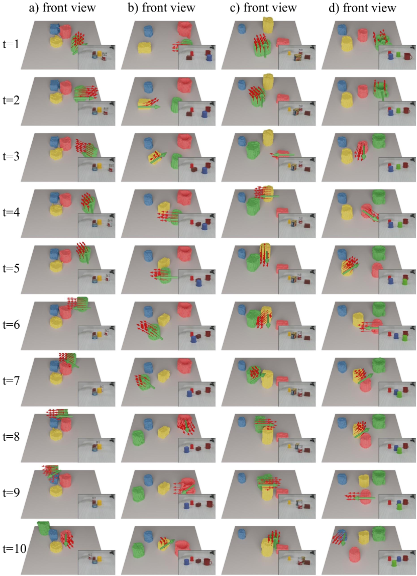
Figure A2 shows additional result for tests cases with different number of objects (two or three object) compare to training cases (four object). While the algorithm is trained only on 4 object cases, it is able handle test case with fewer objects by predicting empty mask for additional object channels.
Appendix A.7 Additional Results and Failure cases
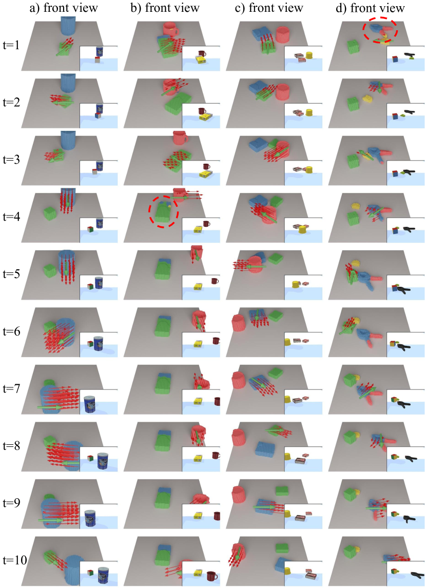
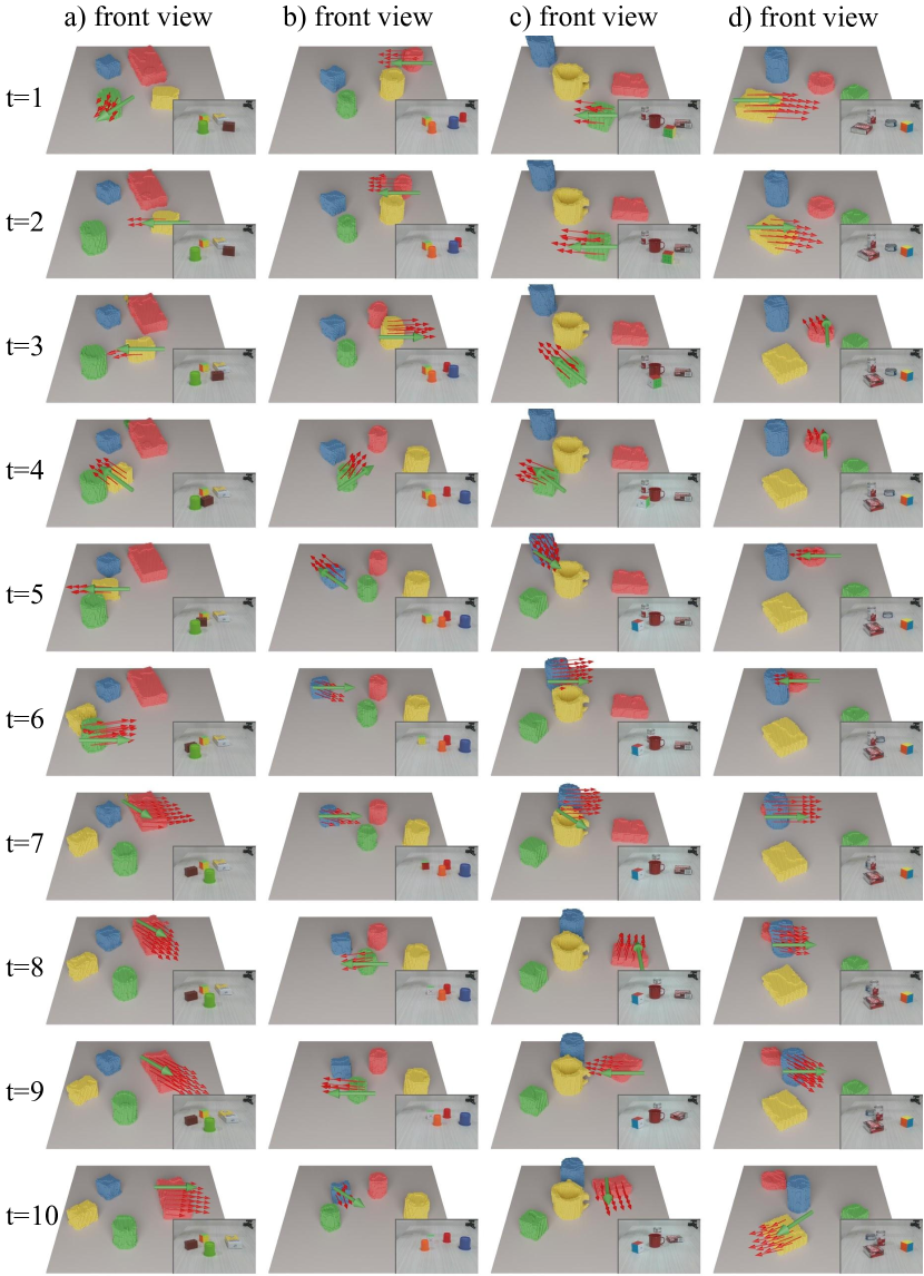
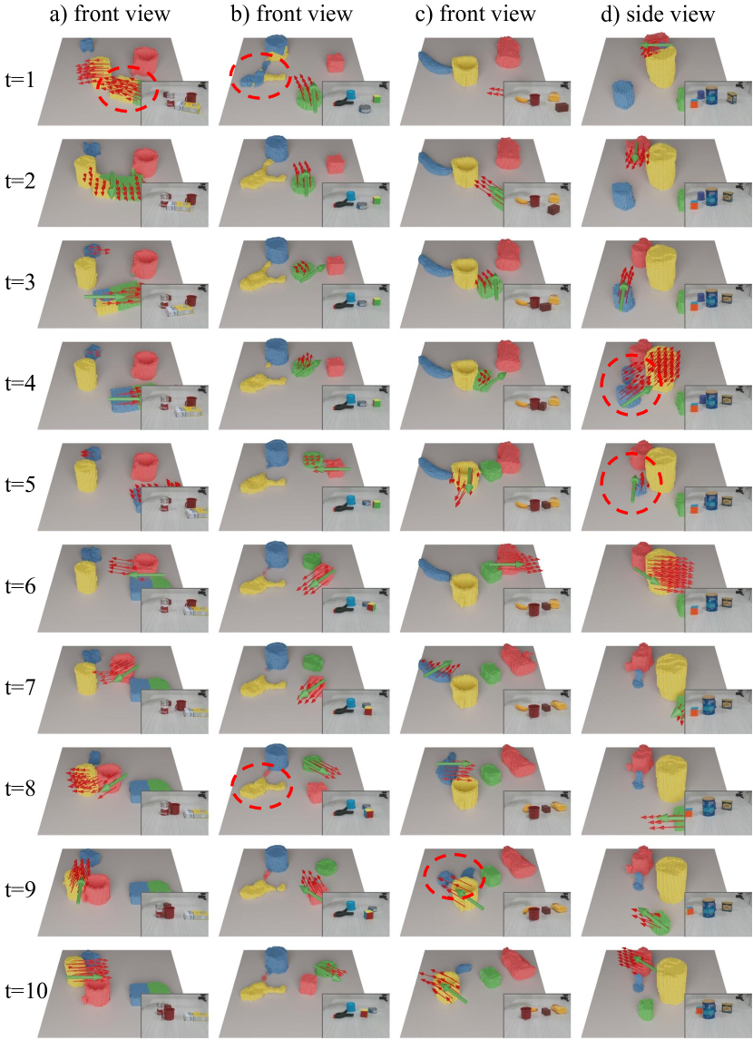
Figure A3 and figure A4 show additional qualitative results on the real-world benchmark. Figure A5 shows some failure cases.
We use simple concatenation for history aggregation, potentially limiting the robustness in the face of incorrect history and long-term history. An interesting future direction might consider using sequences such as LSTM and GRU to handle noises in the history representation. Our algorithm is designed based on the assumption of rigid objects and use SE3 transformations for motion prediction. Future works might consider relaxing this assumption to model deformable or articulated objects. Finally, convolution operations are limited in modeling long-range relationships between objects (e.g., collision), which limits the capacity to model complex interaction and motion, where ideas from graph neural networks may be borrowed to improve this aspect of dynamics modeling.
