Differential Modelling Systematics across the HR Diagram from Asteroseismic Surface Corrections
Abstract
Localised modelling error in the near-surface layers of evolutionary stellar models causes the frequencies of their normal modes of oscillation to differ from those of actual stars with matching interior structures. These frequency differences are referred to as the asteroseismic surface term. Global stellar properties estimated via detailed constraints on individual mode frequencies have previously been shown to be robust with respect to different parameterisations of this surface term. It has also been suggested that this may be true of a broader class of nonparametric treatments. We examine systematic differences in inferred stellar properties with respect to different surface-term treatments, both for a statistically large sample of main-sequence stars, as well as for a sample of red giants, for which no such characterisation has previously been done. For main-sequence stars, we demonstrate that while masses and radii, and hence ages, are indeed robust to the choice of surface term, the inferred initial helium abundance is sensitive to the choice of surface correction. This implies that helium-abundance estimates returned from detailed asteroseismology are methodology-dependent. On the other hand, for our red giant sample, nonparametric surface corrections return dramatically different inferred stellar properties than parametric ones. The nature of these differences suggests that such nonparametric methods should be preferred for evolved stars; this should be verified on a larger sample.
longtable
1 Introduction
Asteroseismology, which has recently become popular owing to the proliferation of high-cadence space photometry, permits precise inference of fundamental properties of field stars, such as their masses and radii. This is in contrast to traditional measurement techniques, which either apply only to special dynamical configurations, such as binary systems, or else operate on stellar populations rather than individual stars. Such inference is predicated on our ability to construct evolutionary models with similar enough structures to the actual stars that their normal modes of oscillation are also similar to the observed normal modes. On the other hand, stellar surfaces are known to be significantly more complicated than we can adequately describe with simple one-dimensional models. In particular, one-dimensional computational treatments of surface magnetic fields and convection cannot be easily reconciled with observational constraints. Consequently, evolutionary models with theoretically identical global properties and interior structures to the observed stars will necessarily yield normal modes that differ slightly from to those that would be measured observationally, owing to modelling error localised to the stellar surface. These frequency differences are generically referred to as the “surface term”, and are predominantly a function of frequency alone; in the Sun, they are known to increase in magnitude with frequency, afflicting high-frequency modes more than low-frequency ones (Brown, 1984; Christensen-Dalsgaard, 1988; Dziembowski et al., 1990).
Ideally, these issues may be ameliorated by explicit hydrodynamical treatments of the stellar surface (e.g. Rosenthal et al., 1999; Sonoi et al., 2015; Mosumgaard et al., 2020), or through detailed analysis of the pulsation eigenfunctions (e.g. Roxburgh, 2015a). However, these prove in many cases to be more computationally expensive than feasible for large-scale modelling. Instead, corrections computed solely from the mode frequencies are much more commonly used. Presently, many approaches to detailed stellar modelling rely on a two-term surface correction proposed in Ball & Gizon (2014, hereafter BG14), of the form
| (1) |
where is the normalisation-independent, dimensionless mode inertia, and the acoustic cutoff frequency may be replaced with up to rescaling of the coefficients and . These are left to vary freely, and are fitted as additional free parameters in determining a best-fitting model. This construction is motivated by the functional analysis of Gough (1990). While the original analysis applied to the Sun (and by extension Sun-like stars), Ball & Gizon (2017) establish the viability of using the BG14 correction for evolved stars as well.
Such a parameterisation of the surface term is not unique, and naturally there exist competing parameterisations (e.g. Kjeldsen et al., 2008; Sonoi et al., 2015). However, the two-term parameterisation of BG14 is more physically motivated than most others, which are instead largely phenomenological in nature, and has been shown empirically to be quite robust. Comparing the performance of different parametric surface corrections (including that of BG14) across the HR diagram in a synthetic test, Schmitt & Basu (2015) concluded that the two-term correction of BG14 yields the most robust agreement with synthetic surface terms generated by perturbing theoretical models. Similarly, Nsamba et al. (2018) and Compton et al. (2018) found the two-term correction of BG14 to be the most likely, in a Bayesian sense, when applied to the Kepler LEGACY sample. Ball & Gizon (2017) arrived at a similar conclusion for a small sample of red giants, as did Ball et al. (2018). Likewise, Jørgensen et al. (2020), who compared seismic masses from various surface corrections with dynamical masses from eclipsing binaries, again concluded that the two-term correction is more robust than other competing parameterisations.
While these works have looked only at various explicit parameterisations of the surface term, there also exist several nonparametric diagnostics. For example, in lieu of the frequencies themselves, Roxburgh & Vorontsov (2003) propose the use of frequency separation ratios as a surface-insensitive set of observational constraints (see also Otí Floranes et al., 2005), although the construction of these quantities introduces correlated errors (Roxburgh, 2018). Roxburgh (2016) also proposes an alternative, less commonly employed phase-matching algorithm. Regarding the use of these various diagnostics and corrections in inferring fundamental stellar properties like masses, radii and compositions, Nsamba et al. (2018) and Basu & Kinnane (2018) demonstrate that such parameter inferences are insensitive to these methodological choices, at least on the main sequence. However, they leave open the question as to whether such robustness continues to obtain for more evolved stars.
Fundamental properties inferred from stellar modelling are known to suffer from various systematic errors owing to both degeneracies in the observational constraints, and uncertainties in the underlying physics. For example, in the absence of a luminosity constraint, posterior distributions returned from grid-based modelling are known to suffer strong correlations between the inferred posterior masses and initial helium abundances, which in turn leads to larger age uncertainties than would be expected from simply propagating the mass uncertainties. Likewise, mixing-length treatments of convective efficiency, which are commonly used in one-dimensional modelling, yield an additional model parameter that is likewise strongly correlated with the inferred masses and radii. In many stellar modelling applications, these parameters are either held fixed (e.g. with a solar-calibrated mixing length) or constrained to reduce the dimensionality of the parameter space Viani et al., 2018, e.g. with a metallicity-mixing length relation,; Moedas et al., 2020, or a metallicity-helium enrichment relation, e.g.; Nsamba et al., 2020.
The imposition of seismic constraints may reduce the overall uncertainties of the inferred quantities, but does not a priori eliminate such degeneracy between model parameters. Rather, seismic constraints may induce new systematic correlations. For example, the large separation is (approximately) a direct constraint on the mean density, and so yields strong degeneracy between the inferred masses and radii. This degeneracy is subtly modified by the surface term; e.g. the use of the BG14 correction is known to modify slightly (Viani et al., 2018). The effects of other surface corrections are less well-studied. In this paper, we investigate the extent and nature of modifications to these systematics introduced by different choices of surface correction.
2 Modelling procedure
The inference of stellar properties from global seismic quantities is known to be affected by a very large number of model parameters, including the initial helium abundance, mixing length parameter, and other choices of model physics — e.g. core or envelope convective overshoot, element diffusion, or the abundance mixture (see e.g. Lebreton et al., 2014; Reese et al., 2016; Silva Aguirre et al., 2017; Nsamba et al., 2018). In this work, we focus largely on the first two parameters. In order to consistently isolate surface-correction-induced systematic effects from those resulting from the underlying stellar models, we adopt a grid-based modelling and Bayesian inference procedure, where likelihoods for all stars in a given sample are inferred from the same set of stellar models. This is as opposed to a sampling scheme dictated by an optimisation-based modelling procedure (e.g. several of the methods in Silva Aguirre et al., 2017) which would have yielded a different set of models for each target, or interpolation-based grid modelling (e.g. Rendle et al., 2019), which is significantly more computationally expensive.
2.1 Cost function
For each star, we should, in principle, compute a log-likelihood function for every model in the grid out of contributions from spectroscopic and seismic inputs, as
| (2) |
This choice of normalisation (in particular, using the reduced instead of total ) was made for consistency with the procedure of McKeever et al. (2019), whose sample of red giants we also use in this work. For the seismic cost term, we choose from one of the following:
However, additional regularisation is necessary when employing the phase-matching or separation-ratio methods, which do not discriminate between stars of different large separations (Roxburgh, 2016). Now, from helioseismology it is known that, at least for the Sun, the surface term decreases with frequency, leaving the lowest-frequency modes least affected (Dziembowski et al., 1990). This is typically also already the case for our best-fitting models using the BG14 surface correction (see e.g. Fig. 1a). Therefore, assuming this to be true for the surface term in general, we include a regularisation term , defined to be the reduced chi-squared associated with the lowest-frequency uncorrected modes:
| (3) |
For our main-sequence sample, we choose , while for our red giants, which have fewer detected modes on average, we choose . This was also done in Basu & Kinnane (2018), who used for all stars.
With the inclusion of this term, our cost function then takes the form
| (4) |
We summarise each of the seismic constraints below. To illustrate these procedures, we show the corresponding quantities associated with one good-fitting stellar model for one of the stars in our sample (KIC 12069449, 16 Cyg B) in Fig. 1.
2.1.1 Parametric surface correction
We adopt the BG14 surface correction, Eq. 1, as our reference parametric surface correction, as it does not require calibration against a reference star, and, as described previously, has been shown to be both more robust and more physically motivated than most other extant parametric surface corrections. In particular, such frequency differences were derived in Gough (1990) from perturbation theory. This does not guarantee the converse — in general, structural differences confined to the near-surface layers may not necessarily result in frequency shifts of these forms. Nonetheless, this is assumed as an ansatz underlying the method.
We construct a reduced- function in the usual manner, as
| (5) |
where the corrected frequencies are as specified in Eq. 1. The parameters and for each stellar model were chosen to minimize this quantity as computed with respect to only radial modes, while the cost functions used in the grid search were computed for each model with respect to those same parameter values, but with all modes included.
2.1.2 Nonparametric surface correction: phase matching
Roxburgh & Vorontsov (2003) constructed a partial-wave eigenvalue equation for stellar p-modes, of the form
| (6) |
with eigenvalues recovered for integer . The quantities and are the partial-wave phase functions of degree associated with the outer and inner boundary, respectively, which may be separately computed by integrating a nonlinear initial value problem from their respective boundaries to a common matching point in the interior.
As per Roxburgh (2016), two stars which differ from each other only in the structure of their outer layers will have identical inner phase functions, and the differences of their outer phase functions , and therefore total phase functions , will be independent of degree (as in Fig. 1b). Again, this does not guarantee the converse: a degree-independent phase-difference function does not in itself guarantee that model differences are localised to the surface. Again, this is nonetheless assumed as part of the method.
Phase functions for modes of each degree are constructed for each model in the grid as
| (7) |
treated as samples of some function of frequency. These are interpolated with a cubic spline, and evaluated at the observed frequencies. For each model we then compute the cost function as the minimum value of
| (8) |
where is is a degree-independent function of frequency with at most parameters. Common choices for such functions include B-splines, or linear combinations of various families of orthogonal polynomials; for our modelling we have opted to follow Roxburgh (2016) in using a linear combination of Chebyshev polynomials.
2.1.3 Nonparametric surface correction: separation ratios
Using Eq. 6, Roxburgh & Vorontsov (2003) further demonstrated that various frequency separation ratios can be related to only the inner partial-wave phase functions of different degrees, evaluated at the same fiducial frequencies. For instance, to leading order,
| (9) |
where the are the inner phase functions of Eq. 6, evaluated at the fiducial frequency . Similar constructions exist for other separation ratios like .
To evaluate the corresponding cost function, we compute these separation ratios separately for the model and observed frequencies. These are to be interpreted as two different functions of frequency (Roxburgh, 2015b). For each model, we interpolate its separation ratio function to the observed fiducial frequencies with a cubic spline (as in Fig. 1c), and evaluate its cost as, e.g.,
| (10) |
We use only and in this manner (as and contain the same information with strongly correlated errors; see Roxburgh, 2018), combining them as . For the dipole separation ratios in particular, we use a three-point rather than five-point construction (see Basu & Kinnane, 2018) to further reduce correlated errors.
2.2 Monte-Carlo recovery of posterior distribution
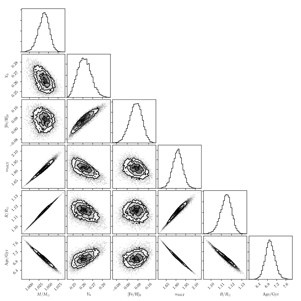
For each star, given a set of spectroscopic constraints and a grid of stellar models, we treat the cost functions computed in the preceding section for each model as a log-likelihood function over the grid: . Given a prior distribution over the parameter space of the grid, this suffices to define a formal posterior distribution
| (11) |
where is inversely proportional to the assumed prior distribution. We may then find weighted averages of, e.g., the stellar mass, by averaging over the grid as e.g.
| (12) |
In principle, this would also permit us to recover higher moments, such as the posterior covariances.
However, depending on the sampling method chosen for the grid, the resulting posterior distribution functions may not be well-behaved; e.g. the model grid may only sample a few discrete values of metallicity, helium abundance, or mixing length. Moreover, strictly speaking the form of Eq. 4, with its various terms normalised differently, cannot be rigorously interpreted as a true log-likelihood function in the usual sense.
To circumvent these difficulties, we estimate the posterior distributions of these parameters using a Monte-Carlo scheme. In particular, we repeat the computation above a large number of times, each time perturbing each of the spectroscopic values from the nominal data by one realisation of independent and identically distributed Gaussian random quantities, with zero mean and with variances given by the nominal measurement errors (as in e.g. Basu et al., 2010). We collect the weighted averages associated with every one of these realisations. Our final estimate of the posterior distribution is then taken to be the distribution of the weighted means returned from all of these realisations. We use realisations for this bootstrapping procedure, which appears to be a good compromise between being large enough to converge to the equlibrium distribution, while also not taking too long to compute for each star. We illustrate the result of this procedure in Fig. 2.
3 Main sequence stars: the LEGACY sample
For studying main-sequence stars, we use the LEGACY sample (Lund et al., 2017), consisting of 66 targets observed with Kepler in short (60 second) cadence. For our modelling, we used spectroscopic constraints derived from high-resolution spectroscopy under the Kepler Follow-up Program (KFOP, Furlan et al., 2018), which was available for 59 out of the 66 stars in the sample. For the remainder, we used the nominal values from the original LEGACY survey (Silva Aguirre et al., 2017). We also use the same detailed mode frequencies as Silva Aguirre et al. (2017).
3.1 Model grid
For the purposes of stellar modelling, we construct a Sobol sequence of elements across a parameter space consisting of the stellar mass , initial helium abundance , initial metallicity , and the mixing length parameter, spaced logarithmically as . For each element in the Sobol sequence we constructed a series of stellar models with mesa r12115, using an Eddington gray atmospheric boundary condition, the mixing-length prescription of Cox & Giuli (1968), the relative heavy-element abundances of Grevesse & Sauval (1998, GS98), with the diffusion and settling of helium and heavy elements as in Burgers (1969), and without any convective overshoot, either in the envelope or core. Performing a solar calibration with these choices of physics yielded a solar-calibrated mixing length of and an initial helium abundance of . A second copy of this Sobol sequence was also constructed with identical values, except for higher metallicities in the range . Only points with were used from this second sequence. Evolutionary tracks were terminated either at a maximum age of 20 Gyr, or 0.5 Gyr after core hydrogen exhaustion, whichever was earlier. Our use of the GS98 solar elemental abundances is motivated by consistency with the community consensus values in the original LEGACY modelling effort (Silva Aguirre et al., 2017), which were also derived with respect to GS98 abundances (except in one case where Grevesse & Noels (1993) abundances were used). These abundances are known to yield better consistency with helioseismic (Antia & Basu, 2006; Basu & Antia, 2008, 2013) and -neutrino (Vinyoles et al., 2017) constraints than do more recent alternatives, such as the abundances of Asplund et al. (2009).
To reduce the computational time required to compute normal mode frequencies, we did the pulsation calculations in a two-step process. Each evolutionary track was run twice: once under default adaptive timestep controls, and a second time with a maximum timestep of 0.03 Gyr. For the first run, the frequencies and inertiae of normal modes within of were computed for using gyre v5.2. The frequencies of the second set of models were then derived by interpolating those of the first set in dimensionless units, as described in Rendle et al. (2019). The mode inertiae were also interpolated logarithmically. In all, the second run yielded a total of about 5 million models.
For a discretely-sampled grid, it is common to check how the inferred parameters change for different values of some model parameters, which are otherwise held fixed. For example, historically could not be observationally constrained, and most isochrone calculations are performed with a fixed value of . On the other hand, seismic radii are known to depend on , and so we might wish to compare the radii obtained from constraining to different values. This is typically done by comparing the properties inferred with respect to only models with , where is a coordinate of the grid. Since doing this with our grid would discard almost all of the Sobol sequence, we cannot apply this procedure directly. Instead, we recognise that such a restriction to the models selected from the grid amounts to constructing means and uncertainties associated with conditional probability distributions. This can otherwise also be effected by applying additional weights to the grid. Selecting a fixed value of with an ordinary grid approximates the analytic expression
| (13) |
so that
| (14) |
For our Sobol-sequence set of evolutionary tracks, we approximate the distribution by using Gaussian weights in Eq. 11 such that
| (15) |
In most of our applications below, the width of the Gaussian is chosen such that the region contains as many sample points as would a slice of a uniformly-sampled discrete grid with the same number of grid points, which works out to about 10% of the Sobol samples in our case.
Parameterising the selection of restricted sets of stellar models as conditional probabilities in this manner also permits more flexible constraints on model selection. For example, since the initial helium abundance is difficult to constrain observationally, it is often determined a priori via a linear enrichment law of the form
| (16) |
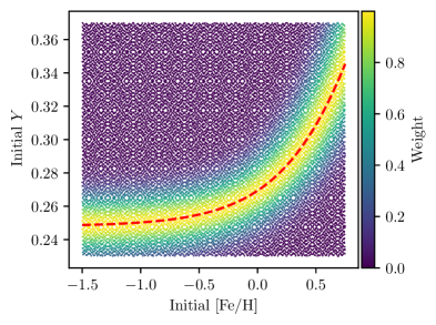
where is set to the primordial value of 0.248, and with the gradient chosen, for example, to yield a star of solar metallicity at the solar age when is at the solar-calibrated value. Comparing the inferred stellar properties returned under such a model selection constraint to those returned where is permitted to vary freely typically necessitates the generation of two different model grids (e.g. Moedas et al., 2020; Nsamba et al., 2020). By contrast, we may instead constrain the initial helium abundance and metallicity to to lie on a hypersurface of constant and (whose projection to the helium-metallicity plane we show in Fig. 3), corresponding to the image of Eq. 16 in the natural coordinates of the Sobol sequence. The distance function used for the Gaussian weights in Eq. 15 is replaced by the minimum Euclidean distance from each grid point to this hypersurface with respect to these coordinates. The resulting weights are also shown in Fig. 3.
3.2 Differences in inferred parameters
We wish to determine if different choices of surface correction impart systematic differences to the resulting estimates of stellar masses, radii, ages, etc. While earlier studies have looked at this in detail on a somewhat ad hoc star-by-star basis (e.g. Nsamba et al., 2018; Compton et al., 2018; Basu & Kinnane, 2018), we opt instead to take a more conservative statistical approach.
Let us consider pairwise differences between the posterior mean masses returned from grid-based modelling with respect to two different surface corrections (e.g. that of BG14 vs. the phase matching method). For each star indexed by , we define a normalised difference in e.g. the stellar mass, as
| (17) |
where and represent the posterior means and standard deviations. If the surface correction does not affect the result of stellar modelling, then in principle this quantity (assembled over all stars in the sample) should be distributed with zero mean. We therefore take this (i.e. the statement that is distributed with zero mean) as our null hypothesis. Our alternate hypothesis is that the population mean is non-zero, so we perform a one-sample two-tailed -test (as done in e.g. Silva Aguirre et al., 2017). As a reminder: the -value returned from such a hypothesis test represents the probability (in a frequentist sense) of making a Type I error — i.e. incorrectly rejecting the null hypothesis. It is customary to define in advance a required level of significance , so as to reject the null hypothesis only for . For the purposes of discussion, we adopt , corresponding to significance on a two-tailed test. However, we will see that many cases are unambiguous.
We show in LABEL:tab:t1 the -values resulting from comparing different surface corrections, including under the effects of different constraints on model selection from the grid (in particular, with a restriction to solar-calibrated mixing length, or a solar-like linear enrichment law). Each entry in the table contains two numbers: the first for a comparison of BG14 vs. phase-matching, and the second for BG14 vs. separation ratios. We do this for the stellar mass, radius, age, and initial helium abundance.
| Quantity | Full Grid | Solar Enrichment (1) | Solar Mixing Length (2) | |
|---|---|---|---|---|
| Mass | ||||
| Radius | ||||
| Age | ||||
We see that most of these -tests do not return significant results by our predetermined criterion, indicating that the relative effects of the three surface terms that we have examined do not matter, on average. Except for the initial helium abundance, even the most significant set of normalised differences (between radii inferred under a solar-like enrichment law) has a distribution whose mean differs from zero only barely discernibly (top panel of Fig. 4). This is consistent with the findings of Compton et al. (2018) and Basu & Kinnane (2018). We have generalised the former by including nonparametric surface corrections in the analysis, and the latter by demonstrating this on a larger, statistical sample.
By contrast, these constraints on model selection are known to significantly affect the estimated stellar properties. To compare the size of these effects, we perform a similar set of tests for systematic differences between inferred parameters returned from each of the above choices of modelling constraints vs. from the full grid, keeping the choice of surface correction consistent. We show the results of these tests in LABEL:tab:t2. Again, each entry in the table consists of two numbers, which are -values for comparisons between a linear enrichment law vs. the full grid, and between a solar-calibrated mixing length vs. the full grid. We see that these differences in model selection contraints yield normalised differences that are clearly nonzero on average (which we illustrate in the middle panel of Fig. 4). The exception to this is the stellar age, which apparently cannot discriminate between these modelling choices. We conclude that the properties of the underlying stellar models have a more significant impact on most inferred global parameters than does the choice of surface correction used when matching them to observations, in agreement with prior work.
| Quantity | BG14 | Phase | Ratios | |
|---|---|---|---|---|
| Mass | ||||
| Radius | ||||
| Age | ||||
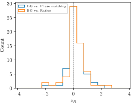
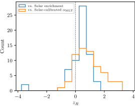
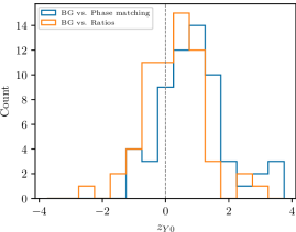
An exception to this is the initial helium abundance, where we find that the method of phase matching yields significantly different values compared to the other two surface corrections, even when the full grid is employed (bottom panel of Fig. 4). Comparing the -values in LABEL:tab:t1 and LABEL:tab:t2, we find that the size of this effect is comparable to that induced by different model selection constraints. Therefore, we conclude that inference of the helium abundance in particular, unlike other model parameters, is sensitive to the choice of surface correction, and therefore methodology-dependent in this respect.
3.3 Differences in correlations between model parameters
As can be seen in Fig. 2, the posterior distributions for various model parameters are correlated with each other (see e.g. Lebreton & Goupil, 2014). We are in particular concerned with the dependences of fundamental stellar properties on the choice of initial helium abundance and the mixing-length parameter , since these model parameters directly affect the other inferred properties, and are also not otherwise well-constrained by direct observations. As the stellar mass is the primary quantity of astrophysical interest in most cases for main-sequence stars, we focus on its correlation with these parameters in particular.
In principle, we could characterise this in terms of the joint second cumulants (i.e. covariances) of the posterior distribution. However, these do not lend themselves easily to physical interpretation. An alternative would be to find the principal axes of the joint posterior distribution (i.e. eigenvectors of the covariance matrix), but this requires that the posterior distributions be symmetric and not curved, which we find to not always be the case.
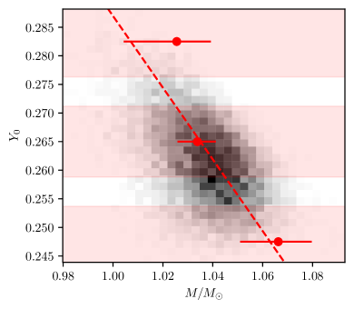
We opt instead to quantify these correlations via the weighted averages of the gradient of the conditional posterior mean of one quantity with respect to another. For example, the conditional posterior mass is in general a function of , and we would like to take the average of the derivative of this function over the values of permitted by the grid. In principle, we should do this by approximating the formal expression
| (18) |
where is the uniform distribution over our input range of, say, the initial helium abundances. Rather than evaluating these derivatives directly, we instead compute using the discretised approximations Eqs. 12 and 13 for several values of , and fit a linear model weighted by the posterior uncertainties. Our final correlation parameter is the gradient of this line. We illustrate this procedure in Fig. 5. We apply the same procedure to find the average derivative of the posterior mass with respect to .
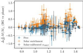
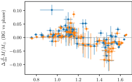
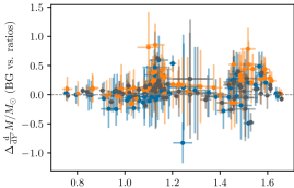
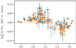
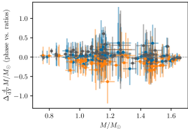
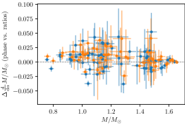
We show these gradients in Fig. 6, as computed with respect to each of the surface corrections we have considered. Broadly speaking, it is difficult to discern any visible structure in the differences between surface corrections, which again suggests that these correlations are a property of the stellar models in the grid rather than on the surface terms used to match them to observational constraints. However, we would like to make this claim more rigorous.
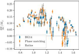
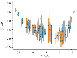
We therefore perform a similar procedure to that in the previous section: for a given pair of surface terms, we construct pairwise differences of the mass-helium correlation parameters for each star, and test the null hypothesis that they are distributed around zero. A significant deviation from this null hypothesis indicate that the two surface corrections result in different systematic correlations. We repeat this procedure for both of the constrained model selection scenarios (solar mixing length and solar enrichment law) as in the previous section.
| Surface corrections | Full Grid | Solar Enrichment | Solar |
|---|---|---|---|
| BG14 vs. phase | |||
| BG14 vs. ratios | |||
| phase vs ratios |
We show these pairwise differences in Fig. 7, colouring points by different model selection constraints. Even visually, it is clear that the imposition of a solar-like linear enrichment law affects each of the surface corrections differently. That is to say, while the correlation between the posterior masses and initial helium abundances depends primarily on the properties of the stellar models, the precise nature of this has a secondary dependence on the choice of surface term. We should qualify that this is in any case a second-order effect: it pertains to the inferred covariances, and not to the global properties per se.
A similar analysis for mass- correlation parameters does not reveal any significant dependence on the surface correction (with a minimum -value of 0.007 among all of the combinations that we examined). However, Fig. 7 suggests that the correlations with respect to returned by the BG14 correction differ from those returned by our other two surface corrections in a mass-dependent manner. Nonetheless, this is once again only a second-order effect. While interesting from a purely statistical perspective, these are likely to be of little consequence for most practical applications. However, in conjunction with our discussion in the previous section, this serves to illustrate again that estimation of the helium abundance in particular, from asteroseismic constraints on evolutionary models, appears to be a highly methodology-dependent affair. While this already known to be the case for other aspects of stellar modelling, we have at least demonstrated that such methodological considerations must also extend to the choice of treatment for the surface term.
3.4 Core diagnostics from separation ratios
One generic problem with all three treatments of the surface term we have considered is that while poor fits (high costs) imply modelling error in the interior structure, the converse may not be true; good fits (low costs) do yield precise estimates of global stellar properties, but they may not necessarily also yield models that match the interior structure of the stars. For instance, structural inversion of the sound speed profiles of 16 Cyg A and B (Bellinger et al., 2017) indicates that stellar models matched to observed frequencies via the BG14 surface correction are known to possess significant internal differences from the structures of the actual stars. On the other hand, Bellinger et al. (2017) also demonstrate that in these cases, the frequency ratios serve as diagnostics of the interior structure, in the sense that for good-fitting models with respect to the BG14 correction, discrepancies with the observed frequency separation ratios still indicate discrepancies in the interior structure.
Given this to be the case, we assume that for otherwise good-fitting models with respect to the BG14 and phase-matching surface corrections, the separation ratios may serve as diagnostics of structural mismatches in the interior. For each of these two methods, let be the value of (Section 2.1.3) associated with the best-fitting model returned by that surface correction. The difference between the two then serves as an informal diagnostic of which method performs better at recovering the internal structure of the actual star; it may be loosely interpreted as a likelihood ratio with respect to being constrained by the separation ratios.
We show these differences on the horizontal axis of Fig. 8a, with the separation-ratio cost function of the best-fitting phase-matching model on the vertical axis. Broadly speaking, most of these values are situated very close to zero, indicating that, as far as the separation-ratio diagnostic is concerned, the best-fitting models selected by both methods are equally good (or equally bad) matches to the interior of the actual star. In Fig. 8(b), we break this down by each of these separation ratios considered separately. This reveals no obvious dependence on degree or on the stellar mass. Since dipole modes probe deeper into the stellar interior than do quadrupole modes, this appears to indicate that any structural mismatches between the best-fitting models selected by the two methods are not preferentially localised.
We also compare the best-fitting model for each method with that selected by using the separation ratios directly; we show the results for the BG14 correction in Fig. 8c, and those for the phase-matching method in Fig. 8d. We see that the phase-matching method returns best-fitting models that uniformly diverge more from the implied interior structure than those selected directly by the separation-ratio constraint. Surprisingly, however, the BG14 correction appears to sacrifice accuracy in matching the dipole mode separation ratios, in exchange for matching the quadrupole mode ratios equally well, on average, as the best-fitting models obtained from fitting the separation ratios directly.
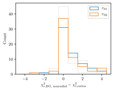
This degree dependence could possibly be a property of our implementation of the BG14 correction, where we have used only radial modes in fitting the free parameters (see Section 2.1.1). To determine if this is the case, we repeated our grid search using radial, dipole, and quadrupole modes to fit the BG14 parameters and , rather than just the radial modes. We show the same log-likelihood-ratios as Fig. 8c in Fig. 9. While including the nonradial modes does appear to alleviate the preference for matching better than , it does so at the expense of overall performance. On average, this procedure appears to select models with internal structures that deviate more from the actual stars than those selected by using only radial modes in fitting the BG14 coefficients, or, for that matter, by using the phase-matching method. We do not have a good explanation for this.
The coefficients of the BG14 parametrisation are found independently for each model by minimising the cost function of Eq. 5. When modelling evolved stars, it often the case that only radial modes are included in this cost function when constraining the BG14 coefficients, since the action of the surface term on mixed modes is nontrivial (see Ball et al., 2018, and Section 4.2), whereas on the main sequence, where all observed modes can be safely assumed to be p-dominated, it is more typical to use modes of all observed degrees to constrain these coefficients. This result suggests that, counterintuitively, the use of only radial modes in this procedure returns better structural matches (as diagnosed by surface-independent separation ratios) even for main-sequence stars, where mode mixing is not ordinarily a concern.
4 Red giants
Unlike the case for main-sequence stars, extant comparisons of surface corrections for red giants have so far investigated only parametric corrections, owing to concerns about the validity of nonparametric methods in the presence of mode mixing (e.g. Ball & Gizon, 2017). We would nonetheless like to investigate how they hold up to parametric methods in any case. We describe rudimentary modifications to mitigate the effects of mode mixing in Section 4.2. Otherwise, we used the same modelling procedure to infer the parameters and posterior distributions of 28 first-ascent red-giant branch (RGB) stars in the open cluster NGC 6791. We use the same spectroscopic properties, measured mode frequencies, stellar model grids, and model frequency calculations as McKeever et al. (2019).
4.1 Model grid
We utilized the pre-existing grid of models from McKeever et al. (2019) to study these relations for red giants. This grid of models was specifically designed to model the open cluster NGC 6791, and is thus more limited in mass range than our main sequence models. The grid was constructed with mesa r10108, using an Eddington gray atmosphere, the mixing-length prescription of Cox & Giuli (1968), the gravitational settling prescription of Thoul et al. (1994), the elemental abundances of Grevesse & Sauval (1998), and with a small amount of convective overshoot (). The grid was discretely sampled at in steps of , in steps of (with two additional intermediate grid points bracketing the central value), in steps of , and in steps of . This discrete sampling meant that we were unfortunately unable to restrict our model selection to e.g. a fixed relation, as we did for our main-sequence stars with Sobol sampling. More details about the grid can be found in the original paper.
4.2 Effects of mixed-mode coupling
The validity of both of the nonparametric methods that we have examined relies on a partial-wave eigenvalue equation depending only on the p-mode radial order . They therefore apply only to uncoupled p-modes, i.e. in the absence of g-mode coupling. In evolved stars, however, this coupling perturbs the frequencies of nonradial p-modes that are close to resonance with internal g-modes of the same degree through the avoided-crossing phenomenon.
The most p-dominated mixed modes returned from observed oscillation power spectra are known to correspond to model mixed modes that achieve maximum visibility, as parameterised by the inverse inertia (e.g. Dupret et al., 2009; Aerts et al., 2010). As demonstrated in Ong & Basu (2020), these occur close to the isolated -mode frequencies (in the sense of Aizenman et al., 1977), which are constructed to yield pure pressure-mode oscillations with no mixing from interior gravity waves. The isolated eigenvalue problem for -modes admits a similar characterisation to uncoupled p-modes in terms of inner and outer partial waves, despite being technically inequivalent. In principle, were these modes observationally accessible, they could be used to construct separations ratios in the same manner, constrained against those constructed from model -modes. However, the measured mode frequencies (which cannot be isolated) will necessarily differ from those of the true -modes owing to mode bumping from the avoided-crossing phenomenon (e.g. Deheuvels & Michel, 2011; Mosser et al., 2012). These deviations are most pronounced with the dipole modes, where the coupling is strongest and the g-mode period spacing is largest (e.g. Pinçon et al., 2020; Jiang et al., 2020); these dipole modes are in turn used in the computatation of all of the standard separation ratios.
As such, we do not use the dipole separation ratios and as a constraint in modelling the red giant sample. On the other hand, frequency separations and separation ratios are known to have been successfully derived from red giants, and employed to obtain good agreement with stellar modelling, where these quantities are computed from the most p-dominated quadrupole mixed modes (cf. Huber et al., 2010; White et al., 2011; Broomhall et al., 2014). This is possible because the - coupling for quadrupole modes is much weaker than for dipole modes; for further discussion of this, see Appendix A. Consequently, we do assume that the observed quadrupole modes are representative of the mode frequencies. Assuming this to be the case, we computed using the modified definition (see Roxburgh, 2016, Eq. 20):
| (19) |
As before, these are treated as functions of frequency, with model quantities interpolated to the observed radial mode frequencies for the purposes of computing cost functions. While isochrones on the - diagram (with this modified definition) have been shown to yield good constraints on main-sequence stellar ages in numerical studies (White et al., 2011), the behaviour of these ratios for evolved stars is largely unexplored. We include it for completeness in comparison with our main-sequence sample.
This issue of mode mixing also afflicts the phase-matching algorithm, where the constructed phase differences collapse to a single function only when comparing two sets of -modes (or uncoupled p-modes). Again, we exclude dipole modes from the phase-matching computation for red giants.
Finally, while mixed-mode resonances resulting in avoided crossings should in principle be determined strictly after the application of the surface correction to the uncoupled -mode frequencies, the BG14 correction is typically applied directly to the model mixed modes instead (i.e. after, and not before, accounting for coupling to g-modes). Ball et al. (2018) demonstrate that these two operations do not commute. Nonetheless, they also show that the parameterisation of BG14 remains sufficiently applicable to the uncoupled -mode frequencies to permit their use in stellar modelling as well, assuming again that these -modes can be accurately estimated. For this reason, and for consistency with both of our nonparametric methods, we again only use quadrupole modes for analysing these red giants.
4.3 Results
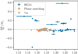
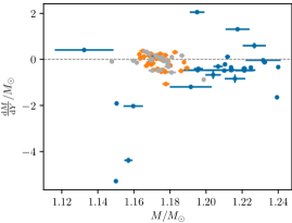
Unlike the case of main-sequence stars, we find that different choices of surface correction yield qualitatively different parameter inferences, even to leading order. We show in Fig. 10 the distribution of inferred masses, and corresponding correlation parameters, as done in Fig. 6. It is clear that both of the nonparametric algorithms return a considerably smaller spread in the inferred stellar masses than does the BG14 correction, although on average the pairwise normalised differences do not differ very significantly from zero (as listed in LABEL:tab:rg). Moreover, the results from both nonparametric surface treatments are highly consistent with each other. This is also the case for other inferred parameters, such as the initial helium abundances and stellar ages.
| Quantity | BG14 vs. phase | BG14 vs. | phase vs. | |
|---|---|---|---|---|
| Mass | ||||
| Radius | ||||
| Age | ||||
In all of these cases, we have modelled each star separately, and so have not constrained the masses to be similar to each other. Nonetheless, seeing as all of these stars are from the same open cluster, all first-ascent red giants should be of essentially the same age and composition, and therefore mass. Consequently, we should prefer a smaller spread in the stellar masses a priori. It is therefore quite astrophysically significant that nonparametric treatments of the surface term should return so much less scatter than the BG14 correction. The most likely reason for this is that the BG14 correction permits far more flexibility than strictly required to describe the surface term in such evolved stars: while the surface properties of main-sequence stars may exhibit significant differences as a matter of mass, age, and composition, all red giants are essentially similar (being almost fully convective).
This result is qualitatively different from that of Jørgensen et al. (2020), who studied different parametric surface corrections for the open clusters NGC 6791 and NGC 6819, where it was found that various parametric surface corrections all yielded comparable scatter in the inferred masses for both clusters. We note that our observed scatter in the inferred masses from the BG14 correction is consistent with previous studies of NGC 6791 (McKeever et al., 2019; Jørgensen et al., 2020) using the same BG14 surface correction. In particular, it is consistent with with results from the grid used in Jørgensen et al. (2020), which was computed over a considerably larger range of stellar masses (0.7 to 2.5 ) and used a different set of physical prescriptions. In our analysis of nonparametric treatments of the surface term, we have taken care to hold constant all other properties of both the grid and the inference methodology. Therefore, we can attribute the markedly reduced scatter in the inferred masses in the other cases solely to the choices of (nonparametric) surface correction. Corollarily, this may suggest that parametric treatments of the surface term, in general, may potentially overfit frequency differences in evolved stars.
Finally, Fig. 10 also shows that the dependence of the inferred masses on the model parameters and is also differently distributed (on the vertical axes) between the three surface corrections we have considered. Unfortunately, as we have noted earlier, the discretised nature of the model grid of McKeever et al. (2019) does not permit us to examine the effects of more sophisticated constraints on model selection, as we did with the LEGACY sample.
5 Discussion and Conclusion
Asteroseismic analysis requires that the surface term be accounted for when using detailed mode frequencies as a modelling constraint; there are many competing proposals for how this is to be done. Previous works have established that the inferred values of many stellar parameters using asteroseismic inputs are robust to different choices of parametric seismic surface corrections, both on the main sequence (Compton et al., 2018; Nsamba et al., 2018) and for evolved stars (Ball & Gizon, 2017; Ball et al., 2018; Jørgensen et al., 2020). On the other hand, there exists a different class of surface corrections, which are nonparametric and motivated from theoretical rather than phenomenological considerations. Nsamba et al. (2018) shows the method of separation ratios, in particular, to be in agreement with other parametric corrections for some Kepler main-sequence stars, while Basu & Kinnane (2018) demonstrated this to also be the case for the phase-matching method as well, albeit on a small sample. We show that these results continue to hold, in a statistical sense, on the full Kepler LEGACY sample. The exception to this is the initial helium abundance, where one of the surface corrections we have examined, the method of phase matching, yields statistically significant differences from the more commonly employed parametric corrections. This suggests that presently ongoing efforts to constrain helium abundances from TESS asteroseismology will be sensitive to the choice of surface correction, which should now be a new methodological consideration for these and future studies (e.g. for the PLATO mission). On the other hand, the phase-matching method in particular is not commonly used for stellar modelling, precisely because of its slightly more computationally expensive nonparametric structure. Further investigation will be necessary to determine if this additional investment will be worth the expense.
Other mixing processes, such as core over/undershoot, are often also invoked as additional free parameters in detailed seismic modelling in order to yield better structural matches, particularly with stars exhibiting convective cores. Although we do not examine the effects of varying these in this work, we are able to demonstrate, in a restricted sense, that their interaction with the surface term is minor, and that the different surface-term prescriptions form behave similarly (see Appendix B).
We have also shown that the situation is drastically different for red giant stars in our NGC 6791 sample, where nonparametric treatments of the surface term yield qualitatively different mass estimates compared to the parametric BG14 correction: inferences for individual stars appear to be more precise, and we also obtain far less statistical scatter when considering the sample of parameters returned from modelling each star in a open cluster separately. To our knowledge, this is the first comparison between parametric and nonparametric treatments of the surface term for evolved stars. It is tempting to conclude from this that such methods should be preferred when modelling these evolved stars. However, this would be a hasty generalisation, given that we have only studied a single open cluster. Further investigation of this nature, repeating this analysis for red giants in other open clusters (e.g. NGC 6819) for which detailed asteroseismology is also available, must be done before any general conclusions about red giants may be drawn.
The phase-matching and separation-ratio methods are not commonly applied to red giants. While we have demonstrated their viability as applied to only quadrupole mixed modes (assumed to be weakly coupled to the inner g-mode cavity), more theoretical work may be required to also include dipole modes in the constraints, where the mixing with the g-mode cavity is known to have a more pronounced effect (see Appendix A).
Appendix A Relative coupling strengths of dipole vs. quadrupole mixed modes
We wish to demonstrate that, at least for our red giant sample, the - coupling for quadrupole modes is sufficiently weak that and may be meaningfully estimated from the observed p-dominated mixed modes. To do this, we will need the following facts:
-
1.
The red giants in our NGC 6791 sample are all close to the RGB bump.
-
2.
Mode coupling between the and cavities admits a functional description with coupling and norm matrices that yield a Hermitian eigenvalue problem, which we write in block matrix form as
(A1) with explicit expressions for these block matrix elements given in Ong & Basu (2020) as integrals against the isolated eigenfunctions. In particular, let us consider the coupling between a single mode and a single mode, so that this eigenvalue problem takes the form
(A2) with eigenvalues , where is the - coupling strength and is the volume overlap integral of their eigenfunctions. Without loss of generality, we choose a normalisation of the eigenfunctions so that both are positive. It can be shown that the perturbation to the eigenvalues with respect to the uncoupled values (e.g. ) is largest at resonance, where , yielding . This is a strict upper bound, so that in general . In turn, this yields an upper bound on the mode bumping as .
-
3.
In practice, the true mode bumping for any given mode will on average also be smaller than this upper bound, since the and modes evolve monotonically in different directions along the RGB, and so do not stay in resonance for long. Only modes whose eigenvalues are sufficiently close, as defined by a characteristic pairwise resonance width (i.e. ), will have their frequencies significantly perturbed through an avoided crossing. This resonance width also scales with .
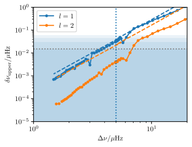
We plot this quantity in Fig. 11 as a function of for the first RGB ascent of a 1.18 MESA evolutionary track below, for the dipole and quadrupole modes closest to . We mark the location of the RGB bump with a vertical dotted line, and we mark out a representative value of the mode frequency measurement error with a horizontal dotted line, with shaded regions for integer multiples thereof to guide the eye. Finally, we mark out the local -mode frequency spacing evaluated at , with dashed lines.
With respect to this diagram, we make the following observations:
-
•
The coupling strength, and so the maximum possible frequency perturbation from mode bumping via the avoided crossing phenomenon, is an order of magnitude weaker for quadrupole modes than dipole modes.
-
•
The resonance widths for dipole modes are comparable to the -mode spacing, but for quadrupole modes they are much smaller than the -mode spacing. Consequently, whereas dipole modes near will be close to resonance with at least one mode at any given time, a quadrupole mode must be fortuitiously in resonance with the underlying -modes, in order for the most p-dominated mixed mode corresponding to it to have its frequency significantly differ from the uncoupled value.
-
•
Even were this to be the case, the magnitude of this frequency perturbation is bounded from above. For the stars in our RGB sample (Hz), the quadrupole upper bound is smaller than, or at most comparable to, the frequency measurement error. That is to say, for the majority of these stars, the observational data cannot distinguish between the uncoupled quadrupole modes and the worst-case bumped frequencies of the most p-dominated quadrupole mixed modes.
Appendix B Sensitivity to overshoot
In this work, we have restricted the choice of physics used in the stellar evolution, since our interest does not lie in accurately estimating stellar properties per se, but rather in isolating the effects of changing the input physics from those of using a different surface correction prescription. For this purpose we have adopted a uniform set of model physics, so that any differences in the inferred properties arise solely from differences in the surface corrections.
Nonetheless, we wish to demonstrate that surface-term-driven systematic effects are largely separable from those arising from different treatments of core overshoot in particular. For this demonstration, we will consider the single star KIC 12258514, which is a LEGACY star that is know to have a convective core. We use the model grid of Viani & Basu (2020), which was constructed with YREC (Demarque et al., 2008). The overshoot parameter was allowed to vary freely in this grid, and was discretely sampled. We apply the modelling procedure of that work — i.e. likelihood-weighted averaging — appropriately modified to include the regularisation term and different surface corrections used in this work, to each of these different subgrids, corresponding to different values of . We show the conditional posterior masses resulting from this procedure in Figure 12. The data points are offset horizontally by surface correction to permit easy visual comparison, and are sized by the maximum of the likelihood function for each subgrid (larger points indicate lower minimum , which are more likely).
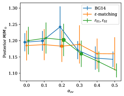
With respect to this figure, we observe the following:
-
•
For each choice of surface correction, the overall variation in the conditional posterior masses (as the overshoot parameter is varied) is in any case comparable to the inferred posterior mass error.
-
•
For each adopted value of the overshoot parameter, the variation in posterior mass between surface corrections is also comparable to the inferred posterior mass error.
Viani & Basu (2020) created independent model grids for each star, making it, unfortunately, difficult to do a population-wide comparison of the kind that we have sought to do in this work. While this result is not necessarily representative of all stars in the sample, it serves to demonstrate that any interaction between surface corrections and overshoot is likely to be small for stars considered individually (as in Compton et al., 2018; Basu & Kinnane, 2018), and hence that these parameter inferences are likely robust to the surface term even when overshoot is varied.
References
- Aerts et al. (2010) Aerts, C., Christensen-Dalsgaard, J., & Kurtz, D. W. 2010, Asteroseismology (Berlin: Springer)
- Aizenman et al. (1977) Aizenman, M., Smeyers, P., & Weigert, A. 1977, A&A, 58, 41
- Antia & Basu (2006) Antia, H. M., & Basu, S. 2006, ApJ, 644, 1292, doi: 10.1086/503707
- Asplund et al. (2009) Asplund, M., Grevesse, N., Sauval, A. J., & Scott, P. 2009, ARA&A, 47, 481, doi: 10.1146/annurev.astro.46.060407.145222
- Astropy Collaboration et al. (2013) Astropy Collaboration, Robitaille, T. P., Tollerud, E. J., et al. 2013, A&A, 558, A33, doi: 10.1051/0004-6361/201322068
- Ball & Gizon (2014) Ball, W. H., & Gizon, L. 2014, A&A, 568, A123, doi: 10.1051/0004-6361/201424325
- Ball & Gizon (2017) —. 2017, A&A, 600, A128, doi: 10.1051/0004-6361/201630260
- Ball et al. (2018) Ball, W. H., Themeßl, N., & Hekker, S. 2018, MNRAS, 478, 4697, doi: 10.1093/mnras/sty1141
- Basu & Antia (2008) Basu, S., & Antia, H. M. 2008, Phys. Rep., 457, 217, doi: 10.1016/j.physrep.2007.12.002
- Basu & Antia (2013) Basu, S., & Antia, H. M. 2013, in Journal of Physics Conference Series, Vol. 440, Journal of Physics Conference Series, 012017
- Basu et al. (2010) Basu, S., Chaplin, W. J., & Elsworth, Y. 2010, ApJ, 710, 1596, doi: 10.1088/0004-637X/710/2/1596
- Basu & Kinnane (2018) Basu, S., & Kinnane, A. 2018, ApJ, 869, 8, doi: 10.3847/1538-4357/aae922
- Bellinger et al. (2017) Bellinger, E. P., Basu, S., Hekker, S., & Ball, W. H. 2017, ApJ, 851, 80, doi: 10.3847/1538-4357/aa9848
- Broomhall et al. (2014) Broomhall, A. M., Miglio, A., Montalbán, J., et al. 2014, MNRAS, 440, 1828, doi: 10.1093/mnras/stu393
- Brown (1984) Brown, T. M. 1984, Science, 226, 687, doi: 10.1126/science.226.4675.687
- Burgers (1969) Burgers, J. M. 1969, Flow Equations for Composite Gases (London: Academic Press)
- Christensen-Dalsgaard (1988) Christensen-Dalsgaard, J. 1988, in Advances in Helio- and Asteroseismology, ed. J. Christensen-Dalsgaard & S. Frandsen, Vol. 123, 3
- Compton et al. (2018) Compton, D. L., Bedding, T. R., Ball, W. H., et al. 2018, MNRAS, 479, 4416, doi: 10.1093/mnras/sty1632
- Cox & Giuli (1968) Cox, J. P., & Giuli, R. T. 1968, Principles of Stellar Structure (Cambridge: Cambridge Scientific Publishers)
- Deheuvels & Michel (2011) Deheuvels, S., & Michel, E. 2011, A&A, 535, A91, doi: 10.1051/0004-6361/201117232
- Demarque et al. (2008) Demarque, P., Guenther, D. B., Li, L. H., Mazumdar, A., & Straka, C. W. 2008, Ap&SS, 316, 31, doi: 10.1007/s10509-007-9698-y
- Dupret et al. (2009) Dupret, M. A., Belkacem, K., Samadi, R., et al. 2009, A&A, 506, 57, doi: 10.1051/0004-6361/200911713
- Dziembowski et al. (1990) Dziembowski, W. A., Pamyatnykh, A. A., & Sienkiewicz, R. 1990, MNRAS, 244, 542
- Foreman-Mackey (2016) Foreman-Mackey, D. 2016, JOSS, 1, 24, doi: 10.21105/joss.00024
- Furlan et al. (2018) Furlan, E., Ciardi, D. R., Cochran, W. D., et al. 2018, ApJ, 861, 149, doi: 10.3847/1538-4357/aaca34
- Gough (1990) Gough, D. 1990, in Progress of Seismology of the Sun and Stars, ed. Y. Osaki & H. Shibahashi (Berlin, Heidelberg: Springer Berlin Heidelberg), 281–318
- Grevesse & Noels (1993) Grevesse, N., & Noels, A. 1993, Physica Scripta Volume T, 47, 133, doi: 10.1088/0031-8949/1993/T47/021
- Grevesse & Sauval (1998) Grevesse, N., & Sauval, A. J. 1998, Space Sci. Rev., 85, 161, doi: 10.1023/A:1005161325181
- Harris et al. (2020) Harris, C. R., Millman, K. J., van der Walt, S. J., et al. 2020, Nature, 585, 357
- Huber et al. (2010) Huber, D., Bedding, T. R., Stello, D., et al. 2010, ApJ, 723, 1607, doi: 10.1088/0004-637X/723/2/1607
- Jiang et al. (2020) Jiang, C., Cunha, M., Christensen-Dalsgaard, J., & Zhang, Q. 2020, MNRAS, doi: 10.1093/mnras/staa1285
- Jones et al. (2001–) Jones, E., Oliphant, T., Peterson, P., et al. 2001–, SciPy: Open source scientific tools for Python. http://www.scipy.org/
- Jørgensen et al. (2020) Jørgensen, A. C. S., Montalbán, J., Miglio, A., et al. 2020, MNRAS, 495, 4965, doi: 10.1093/mnras/staa1480
- Kjeldsen et al. (2008) Kjeldsen, H., Bedding, T. R., & Christensen-Dalsgaard, J. 2008, ApJ, 683, L175, doi: 10.1086/591667
- Lebreton & Goupil (2014) Lebreton, Y., & Goupil, M. J. 2014, A&A, 569, A21, doi: 10.1051/0004-6361/201423797
- Lebreton et al. (2014) Lebreton, Y., Goupil, M. J., & Montalbán, J. 2014, in EAS Publications Series, Vol. 65, EAS Publications Series, 177–223
- Lund et al. (2017) Lund, M. N., Silva Aguirre, V., Davies, G. R., et al. 2017, ApJ, 835, 172, doi: 10.3847/1538-4357/835/2/172
- McKeever et al. (2019) McKeever, J. M., Basu, S., & Corsaro, E. 2019, ApJ, 874, 180, doi: 10.3847/1538-4357/ab0c04
- McKinney (2010) McKinney, W. 2010, in Proceedings of the 9th Python in Science Conference, ed. S. van der Walt & J. Millman, 51 – 56
- Moedas et al. (2020) Moedas, N., Nsamba, B., & Clara, M. T. 2020, arXiv e-prints, arXiv:2007.03362. https://arxiv.org/abs/2007.03362
- Mosser et al. (2012) Mosser, B., Goupil, M. J., Belkacem, K., et al. 2012, A&A, 540, A143, doi: 10.1051/0004-6361/201118519
- Mosumgaard et al. (2020) Mosumgaard, J. R., Jørgensen, A. C. S., Weiss, A., Silva Aguirre, V., & Christensen-Dalsgaard, J. 2020, MNRAS, 491, 1160, doi: 10.1093/mnras/stz2979
- Nsamba et al. (2018) Nsamba, B., Campante, T. L., Monteiro, M. J. P. F. G., et al. 2018, MNRAS, 477, 5052, doi: 10.1093/mnras/sty948
- Nsamba et al. (2020) Nsamba, B., Moedas, N., Campante, T. L., et al. 2020, MNRAS, doi: 10.1093/mnras/staa3228
- Ong & Basu (2020) Ong, J. M. J., & Basu, S. 2020, ApJ, 898, 127, doi: 10.3847/1538-4357/ab9ffb
- Otí Floranes et al. (2005) Otí Floranes, H., Christensen-Dalsgaard, J., & Thompson, M. J. 2005, MNRAS, 356, 671, doi: 10.1111/j.1365-2966.2004.08487.x
- Paxton et al. (2011) Paxton, B., Bildsten, L., Dotter, A., et al. 2011, ApJS, 192, 3, doi: 10.1088/0067-0049/192/1/3
- Paxton et al. (2013) Paxton, B., Cantiello, M., Arras, P., et al. 2013, ApJS, 208, 4, doi: 10.1088/0067-0049/208/1/4
- Paxton et al. (2018) Paxton, B., Schwab, J., Bauer, E. B., et al. 2018, ApJS, 234, 34, doi: 10.3847/1538-4365/aaa5a8
- Pinçon et al. (2020) Pinçon, C., Goupil, M. J., & Belkacem, K. 2020, A&A, 634, A68, doi: 10.1051/0004-6361/201936864
- Price-Whelan et al. (2018) Price-Whelan, A. M., Sipőcz, B. M., Günther, H. M., et al. 2018, AJ, 156, 123, doi: 10.3847/1538-3881/aabc4f
- Reese et al. (2016) Reese, D. R., Chaplin, W. J., Davies, G. R., et al. 2016, A&A, 592, A14, doi: 10.1051/0004-6361/201527987
- Rendle et al. (2019) Rendle, B. M., Buldgen, G., Miglio, A., et al. 2019, MNRAS, 484, 771, doi: 10.1093/mnras/stz031
- Rosenthal et al. (1999) Rosenthal, C. S., Christensen-Dalsgaard, J., Nordlund, Å., Stein, R. F., & Trampedach, R. 1999, A&A, 351, 689. https://arxiv.org/abs/astro-ph/9803206
- Roxburgh (2015a) Roxburgh, I. W. 2015a, A&A, 574, A45, doi: 10.1051/0004-6361/201425289
- Roxburgh (2015b) —. 2015b, A&A, 584, A71, doi: 10.1051/0004-6361/201527447
- Roxburgh (2016) —. 2016, A&A, 585, A63, doi: 10.1051/0004-6361/201526593
- Roxburgh (2018) —. 2018, arXiv e-prints, arXiv:1808.07556. https://arxiv.org/abs/1808.07556
- Roxburgh & Vorontsov (2003) Roxburgh, I. W., & Vorontsov, S. V. 2003, A&A, 411, 215, doi: 10.1051/0004-6361:20031318
- Schmitt & Basu (2015) Schmitt, J. R., & Basu, S. 2015, ApJ, 808, 123, doi: 10.1088/0004-637X/808/2/123
- Silva Aguirre et al. (2017) Silva Aguirre, V., Lund, M. N., Antia, H. M., et al. 2017, ApJ, 835, 173, doi: 10.3847/1538-4357/835/2/173
- Sonoi et al. (2015) Sonoi, T., Samadi, R., Belkacem, K., et al. 2015, A&A, 583, A112, doi: 10.1051/0004-6361/201526838
- Thoul et al. (1994) Thoul, A. A., Bahcall, J. N., & Loeb, A. 1994, ApJ, 421, 828, doi: 10.1086/173695
- Townsend & Teitler (2013) Townsend, R. H. D., & Teitler, S. A. 2013, MNRAS, 435, 3406, doi: 10.1093/mnras/stt1533
- Viani & Basu (2020) Viani, L. S., & Basu, S. 2020, arXiv e-prints, arXiv:2009.09344. https://arxiv.org/abs/2009.09344
- Viani et al. (2018) Viani, L. S., Basu, S., Ong, J. M. J., Bonaca, A., & Chaplin, W. J. 2018, ApJ, 858, 28, doi: 10.3847/1538-4357/aab7eb
- Vinyoles et al. (2017) Vinyoles, N., Serenelli, A. M., Villante, F. L., et al. 2017, ApJ, 835, 202, doi: 10.3847/1538-4357/835/2/202
- White et al. (2011) White, T. R., Bedding, T. R., Stello, D., et al. 2011, ApJ, 743, 161, doi: 10.1088/0004-637X/743/2/161