Directional ASR: A new paradigm for E2E multi-speaker speech recognition with source localization
Abstract
This paper proposes a new paradigm for handling far-field multi-speaker data in an end-to-end neural network manner, called directional automatic speech recognition (D-ASR), which explicitly models source speaker locations. In D-ASR, the azimuth angle of the sources with respect to the microphone array is defined as a latent variable. This angle controls the quality of separation, which in turn determines the ASR performance. All three functionalities of D-ASR: localization, separation, and recognition are connected as a single differentiable neural network and trained solely based on ASR error minimization objectives. The advantages of D-ASR over existing methods are threefold: (1) it provides explicit speaker locations, (2) it improves the explainability factor, and (3) it achieves better ASR performance as the process is more streamlined. In addition, D-ASR does not require explicit direction of arrival (DOA) supervision like existing data-driven localization models, which makes it more appropriate for realistic data. For the case of two source mixtures, D-ASR achieves an average DOA prediction error of less than three degrees. It also outperforms a strong far-field multi-speaker end-to-end system in both separation quality and ASR performance.
Index Terms— source localization, source separation, end-to-end speech recognition
1 Introduction
Source localization methods to estimate the direction of the sound sources with respect to the microphone array is an important front-end for many downstream applications. For example, they are an indispensable part of robot audition systems [1, 2] that facilitates interaction with humans. Source localization is used as a pivotal component in the robot audition pipeline to aid source separation and recognition. Recently far-field systems are being designed to process multi-talker conversations like meeting [3] and smart speaker scenarios [4, 5]. Incorporating source localization functionality can enrich such systems by monitoring the location of speakers and also potentially help improve the performance of the downstream automatic speech recognition (ASR) task. Assuming the direction of arrival (DOA) is known, the effectiveness of using features extracted from the ground-truth location for target speech extraction and recognition was shown in [6, 7].
Similar to other front-end tasks, signal processing has been traditionally used to estimate the DOA [8, 9, 10]. Wideband subspace methods like test of orthogonality of projected subspaces (TOPS) have shown promising improvements over narrowband subspace methods like multiple signal classification (MUSIC) but most existing signal processing approaches are not robust to reverberations [11]. Supervised deep learning methods have been successful in making the DOA estimation more robust [12, 11, 13]. However, for real multi-source data like CHiME-5 [4], it is very difficult to get the parallel ground-truth DOA. In such cases, it might be possible to use labels from a different view that are easier to annotate and use it to indirectly optimize the localization model parameters.
There is growing interest in optimizing the front-end speech processing systems with applications-oriented objectives. For example, speech enhancement and separation systems have been trained based on ASR error minimization [14, 15, 16, 17, 18, 19, 20, 7]. The front-end in such systems was encompassed into the ASR framework to train them without parallel clean speech data by using the text transcription view as the labels. MIMO-Speech [20] is a multichannel end-to-end (ME2E) neural network that defines source-specific time-frequency (T-F) masks as latent variables in the network which in turn are used to transcribe the individual sources.
Although MIMO-Speech might implicitly learn localization information, it might not be consistent across frequencies because of narrowband approximation. We propose to further upgrade the explainability factor of the MIMO-Speech system by realizing an explicit source localization function. We call our novel technique directional ASR (D-ASR), which is a new paradigm of joint separation and recognition explicitly driven by source localization. The masking network in MIMO-Speech is expected to directly predict an information rich T-F mask. It is hard to accurately estimate such a mask without the reference signals. In D-ASR, this masking network is replaced with a simpler component that discretizes the possible DOA azimuth angles and estimates the posterior of these angles for each source. This estimated angle can be in turn converted to steering vectors and T-F masks, thereby making the localization function tightly coupled with the other two functionalities of D-ASR. This streamlining makes this method more effective. The estimated angle is tied across the steering vector for all frequency bands and hence this method also has wideband characteristics.
Although D-ASR is trained with only the ASR objective, its evaluation is performed across all three of its expected functionalities. This is possible as the localization and separation intermediate outputs are interpretable in our formulation. The L1 prediction error is used as the DOA metric with MUSIC and TOPS as baselines for this comparison. Source separation and ASR performance are compared with the MIMO-Speech model [21] with objective signal quality and transcription based metrics, respectively.
2 Directional ASR
A block diagram of the proposed D-ASR architecture is shown in Figure 1. The architecture has five blocks and a detailed formulation of these blocks is given in this section.
2.1 Localization Subnetwork
The first block is the localization subnetwork and its goal is to estimate the azimuth angle of the sources. This block in turn has three components: (1) CNN-based phase feature extraction, (2) phase feature masking and, (3) temporal averaging.
Let be the -channel input signal in the short-time Fourier transform (STFT) domain, with , where is the number of frames and is the number of frequency components. The input signal is reverberated, consisting of speech sources with no noise. We assume that is known. The phase spectrum of the multichannel input signal is represented as . This raw phase is passed through the first component of the localization network based on CNN given by to extract phase feature by pooling the channels as follows:
| (1) |
where is the feature dimension. Phase feature will have DOA information about all the sources in the input signal. This is processed by the next component which is a recurrent layer. This component is used to extract source-specific binary masks as follows,
| (2) |
where is the feature mask for source and is the sigmoid activation. This mask segments into regions that correspond to each source.
In this work, we assume that the DOA does not change for the whole utterance. So in the next step we use the extracted phase mask from Eq. (2) to perform a weighted averaging of the phase feature from Eq. (1) to get source-specific summary vectors. This summary vector should encode the DOA information specific to a source and that is why the mask is used as weights to summarize information only from the corresponding source regions.
| (3) |
where is the summary vector for source at dimension , and are the extracted feature mask (for source ) and the phase feature, respectively, at time and feature dimension .
The summary vector, represented in vector form as is passed through a learnable , which converts the summary vector from dimension to the dimension , where is the angle resolution in degrees to discretize the DOA angle. Based on this discretization, we can predict the DOA angle as a multi-class classifier with the softmax operation. From this, we can get the source-specific posterior probability for the possible angle classes as follows,
| (4) | ||||
| (5) | ||||
| (6) |
where is the DOA estimated for source by performing a weighted sum using the estimated posteriors from Eq. (4) and is the angle in radians corresponding to the class . We define the composite function of Eqs. (1)–(6) with learnable parameter as follows:
| (7) |
Note that all of the functions in this section are differentiable.

2.2 Steering Vector & Localization Mask
In this step, the estimated DOAs from Eq. (7) is converted to a steering vector and also optionally to a time-frequency mask to be used for beamforming. First, the steering vector for source and frequency is calculated from estimated DOA . In this work we have used uniform circular arrays (UCA) and the steering vector is calculated as follows,
| (8) | ||||
| (9) |
where is the signed time delay between the -th microphone and the center for source , is the angular location of microphone , is the radius of the UCA and is the speed of sound (343 m/s).
The estimated steering vectors can be sufficient to separate the signals. However, depending on the beamformer used subsequently, we can also use a time-frequency mask and it is estimated as,
| (10) | ||||
| (11) | ||||
| (12) |
where is a sparsity constant, is conjugate transpose, is the multichannel input at time and frequency . An initial estimate of the mask is extracted by passing the directional power spectrum through a softmax function over the source dimension using Eq. (11). The mask is further refined using Eq. (12) to create sparsity and we define this output as the localization mask. Again, all of the operations in this section are differentiable.
2.3 Differentiable Beamformer
As we have both steering vectors from Eq. (9) and masks from Eq. (12), there are many possible beamformers that could be used. We experimented with three options. First, linearly constrained minimum power (LCMP) beamformer [22] given by for source and frequency , is estimated by solving the following equation which requires only the steering vectors,
| (13) | ||||
| (14) |
where is the input spatial covariance matrix (SCM) at frequency . is the constraint matrix whose columns are the estimated steering vectors at frequency , such that the -th column is . is a one-hot vector with the -th element as 1. Alternative to LCMP, we can use MVDR beamformer. The localization masks from Eq. (12) are used to compute the source specific SCM, as follows:
| (15) |
The interference SCM, for source is approximated as like [20] (we experiment only with , so no summation in that case). From the computed SCMs, the -dimensional complex MVDR beamforming filter for source and frequency , is estimated as,
| (16) |
We can also use the MVDR formulation based on reference selection [23], in which case the steering vectors will not be used explicitly. We refer to this beamformer as MVDR-REF and it is estimated as,
| (17) |
where is a one-hot vector to choose a reference microphone and denotes the trace operation.
Once we obtain the beamforming filters from either Eq. (13), Eq. (16) or Eq. (17), we can perform speech separation to obtain the -th separated STFT signal, as follows:
| (18) |
where can be either of LCMP, MVDR or MVDR-REF beamforming coefficients. Again, all the operations in this section are also differentiable. One added advantage of our approach is that we can use a different beamformer during inference to what was used during training. Irrespective of the beamformer used while training, we found that using MVDR-REF while inference gives better separation and ASR performance.
2.4 Feature Transformation & ASR
| (19) | ||||
| (20) |
The separated signal for source from Eq. (18), represented in matrix form as is transformed to a feature suitable for speech recognition by performing log Mel filterbank transformation and utterance based mean-variance normalization (MVN). The extracted feature for source is passed to the speech recognition subnetwork with learnable parameter to get , the token sequence corresponding to source .
As shown in Figure 1, all the components are connected in a computational graph and trained solely based on the ASR objective to learn both in Eq. (7) and in Eq. (20) with the reference text transcriptions as the target. The joint connectionist temporal classification (CTC)/attention loss [24] is used as the ASR optimization criteria. We use the permutation invariant training (PIT) scheme similar to MIMO-Speech [20, 21] to resolve the prediction-target token sequence assignment problem. Optionally, a regularization cross entropy loss for the posteriors in Eq. (4) with a uniform probability distribution as the target can be added. This is to discourage a very sparse posterior distribution and encourage interpolation in Eq. (5), especially when high values of are used.
3 Experiments
3.1 Data & Setup
We simulated 2-speaker mixture data using clean speech from the subset WSJ0 of the wall street journal (WSJ) corpus [25]. For each utterance, we mixed another utterance from a different speaker within the same set, so the resulting simulated data is the same size as the original clean data with 12,776 (si_tr_s), 1,206 (dt_05), and 651 (et_05) utterances for the training, development, and test set respectively. The SMS-WSJ [26] toolkit was used for creating the simulated data with maximum overlap. Image method [27] was used to create the room impulse responses (RIR). Room configurations with the size (length-width-height) ranging from 5m-5m-2.6m to 11m-11m-3.4m were used. A uniform circular array (UCA) with a radius of 5 cm was used. The reverberation time (T60) was sampled uniformly between 0.15s and 0.5s. The two speech sources were placed randomly at a radius of 1.5-3m around the microphone-array center.
Three CNN layers with rectified linear unit (ReLU) activation followed by a feedforward layer were used as defined in Eq. (1). was fixed as “”. One output gate projected bidirectional long short-term memory (BLSTMP) layer with cells was used as defined in Eq. (2). in Eq. (12) was fixed as “0.5”. The encoder-decoder ASR network was based on the Transformer architecture [28] and it is initialized with a pretrained model that used single speaker training utterances from both WSJ0 and WSJ1. Attention/CTC joint ASR decoding was performed with score combination with a word-level recurrent language model from [29] trained on the text data from WSJ. Our implementation was based on ESPnet [30].
The input signal was preprocessed with weighted prediction error (WPE) [31, 32] based dereverberation with a filter order of “10” and prediction delay “3”, only during inference time . The second channel was fixed as the reference microphone for MVDR-REF in Eq. (17). The recently proposed MIMO-Speech with BLSTM front-end and Transformer back-end [21] was used as the 2-source ASR baseline. We used the same ASR subnetwork architecture as D-ASR in MIMO-Speech for a fair comparison. Signal processing based DOA estimation was performed with “Pyroomacoustics” toolkit [33].
3.2 Multi-Source Localization Performance
The estimated azimuth angles (DOA) from our proposed D-ASR method are extracted as intermediate outputs from Eq. (7). We use two popular subspace-based signal processing methods MUSIC and TOPS as baselines. For both, the spatial response is computed and the top two peaks are detected to estimate the DOA. The average absolute cyclic angle difference between the predicted angle and the ground-truth angle in degrees is used as the metric. The permutation of the prediction with the reference that gives the minimum error is chosen.
The results with and without WPE preprocessing are given in Table 1. Results of the D-ASR method with all three possible beamformers while training and different angle resolutions () are shown. All configurations of D-ASR outperforms the baselines. Specifically, LCMP version is significantly better. In the LCMP version of D-ASR, having a higher of 10 works best and it is also robust without WPE. The results of LCMP D-ASR with is shown with and without the additional regularization loss (cross-entropy with uniform distribution as target). Although this regularization doesn’t change the performance much, it helps in faster convergence during training.
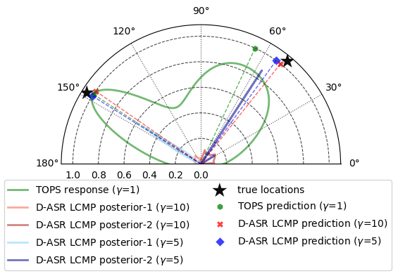
If the posteriors in Eq. (4) were 1-hot vectors, there would have been a discretization error of (for =10) but our prediction error is less than this. This shows that the network uses the posteriors as interpolation weights and hence it is not bounded by the discretization error. Figure 2 shows the localization output for a test example (note that only half of the possible angles are shown as in this case all the predictions were in the top semi-circle). TOPS predicts one of the sources which is at with good precision like the two D-ASR LCMP systems shown but has about a error in predicting the other source at , which the D-ASR systems can estimate again with good precision. The posteriors of D-ASR () trained without the regularization loss predicts a very sparse distribution while for the one with regularization loss and , the distribution is very dense but the prediction with the weighted sum is a bit more accurate.
Method Training Uniform Average L1 Error (degree) Beamformer Regulariza- No WPE WPE tion Dev Test Dev Test MUSIC - 1 - 22.5 24.0 15.6 14.4 MUSIC - 10 - 23.2 21.7 13.5 12.6 TOPS - 1 - 20.0 18.7 11.7 10.1 TOPS - 10 - 20.4 19.4 13.3 10.6 D-ASR LCMP 1 ✓ 20.3 20.8 8.3 7.0 D-ASR LCMP 5 ✓ 3.9 3.6 3.5 3.0 D-ASR LCMP 5 ✗ 8.6 7.7 3.7 3.5 D-ASR LCMP 10 ✓ 3.0 3.0 2.5 2.5 D-ASR MVDR 5 ✓ 11.5 10.4 7.4 7.1 D-ASR MVDR 10 ✓ 20.8 19.9 7.4 6.9 D-ASR MVDR-REF 5 ✓ 14.2 14.5 10.2 10.9
3.3 ASR & Source Separation Performance
Word error rate (WER) is used as the metric for ASR. The signal-to-distortion ratio (SDR) and perceptual evaluation of speech quality (PESQ) scores computed with the dry signal as the reference are used as the metric for source separation. The results are given in Table 2. The LCMP based D-ASR with is used for this evaluation as that performs the best in terms of DOA error. We observed the steering vector based LCMP beamformer to be good at training the D-ASR network as that ensures tighter coupling with the localization subnetwork but once the network parameters are learned it was better to replace the beamformer to be mask-based for inference. So during inference MVDR-REF beamformer was used as mentioned in Section 2.4.
WER (%) SDR (dB) PESQ Dev Test Dev Test Dev Test Clean 2.1 1.6 - - - - Input mixture (ch-1) 105.0 107.1 -0.2 -0.2 1.9 1.9 Oracle binary Mask (IBM) 3.6 3.0 15.7 15.5 2.9 2.9 Oracle DOA Mask (ILM) 4.3 3.7 15.3 15.3 2.9 2.9 MIMO-Speech 6.6 5.1 11.2 11.7 2.6 2.7 D-ASR 5.1 4.1 15.2 15.2 2.9 2.9
The results of the clean single-speaker data with the pretrained ASR model is given in the first row to show a bound for the 2-mix ASR performance. The ASR results of the simulated mixture using the single-speaker model is also shown (WER more than 100% because of too many insertion errors). We perform oracle experiments by directly giving the reference masks to the beamformer. We define an ideal localization mask (ILM) which is basically Eq. (12) calculated by using the ground-truth DOA. The ILM is compared with the ideal binary mask (IBM) that is calculated with the reference clean signal magnitude. The ILM system is slightly worse than IBM but the results show it is a good approximation for IBM, which justifies our approach of obtaining masks from the DOA.
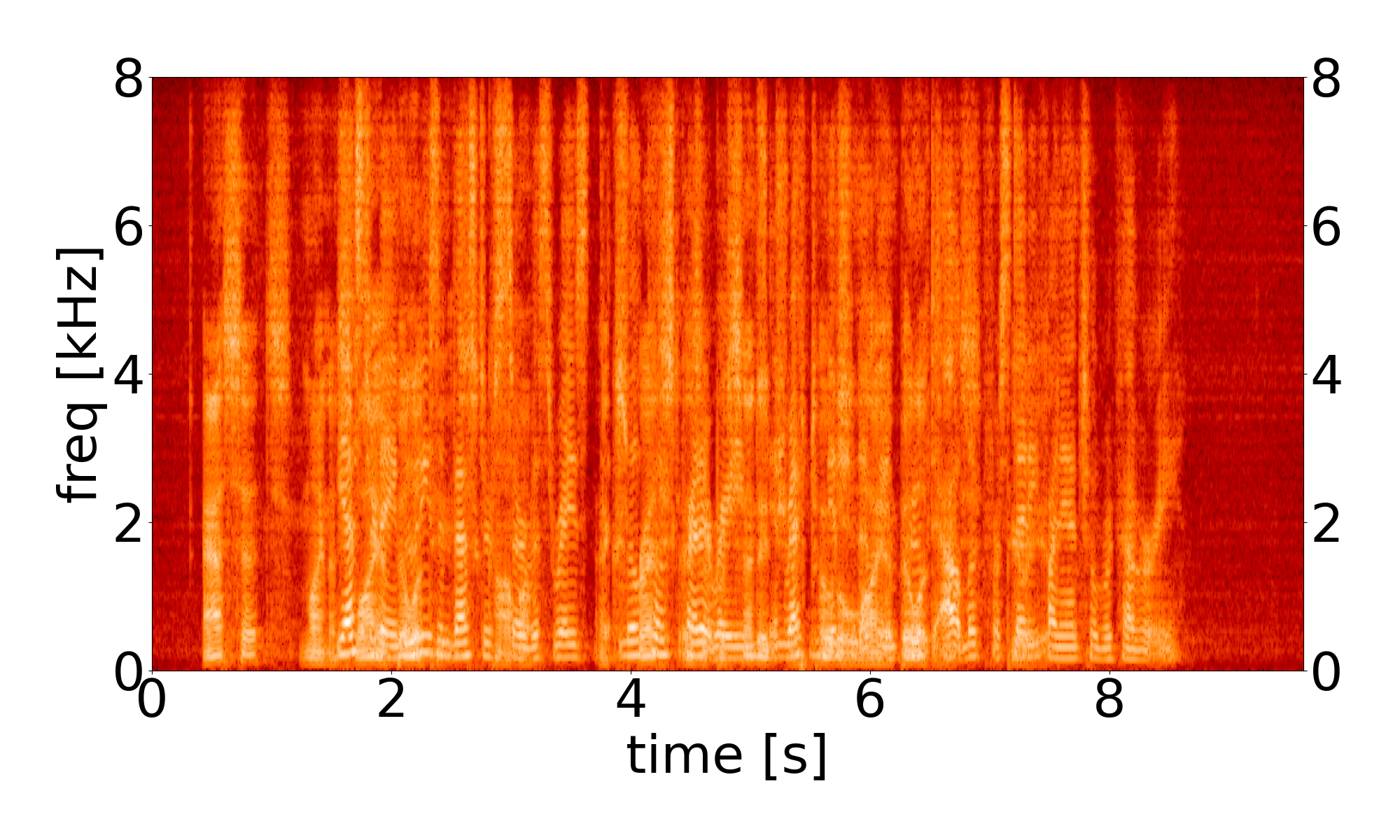
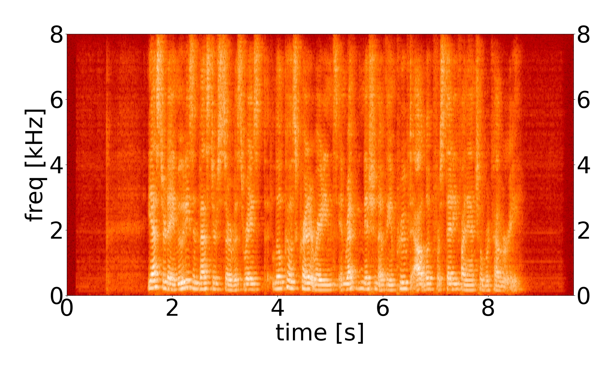
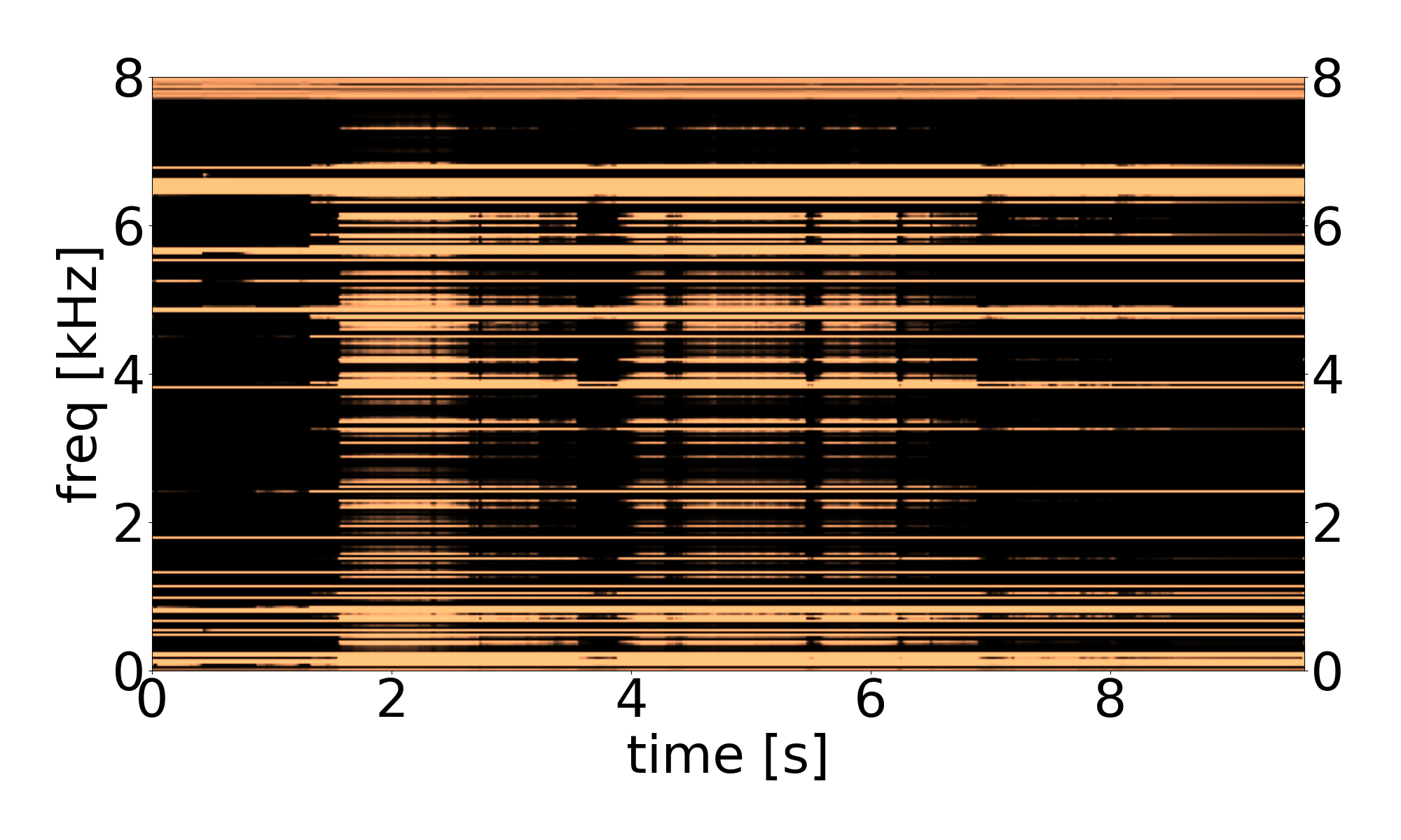
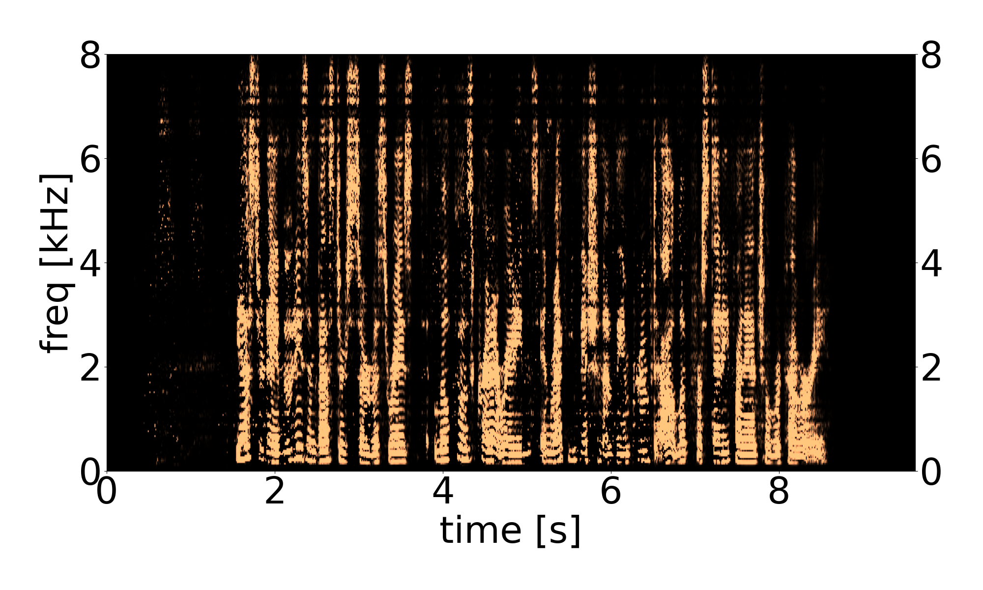
Our proposed D-ASR method outperforms MIMO-Speech with the added advantage of also predicting DOA information. The SDR scores of D-ASR is almost as good as the oracle IBM and it is far superior to MIMO-Speech. An example of the estimated masks comparing D-ASR with MIMO-Speech is shown in Figure 3. In MIMO-Speech as the spectral masks are estimated directly, it is hard for the network to learn this without reference signals. Our approach can provide better masks because we simplify the front-end to just predict angles and then approximate the mask from it. Some audio examples for demonstration are given in https://sas91.github.io/DASR.html
4 CONCLUSION
This paper proposes a novel paradigm to drive far-field speech recognition through source localization. It also serves as a method to learn multi-source DOA from only the corresponding text transcriptions. D-ASR not only makes the existing approaches like MIMO-Speech more interpretable but also performs better in terms of both ASR and speech separation.
References
- [1] K. Nakadai, T. Takahashi, H. Okuno, H. Nakajima, et al., “Design and implementation of robot audition system ‘HARK’ - open source software for listening to three simultaneous speakers,” Advanced Robotics, vol. 24, no. 5-6, pp. 739–761, 2010.
- [2] K. Nakadai, K. Hidai, H. Mizoguchi, H. Okuno, et al., “Real-time auditory and visual multiple-object tracking for humanoids,” in IJCAI, 2001, pp. 1425–1432.
- [3] T. Yoshioka, I. Abramovski, C. Aksoylar, Z. Chen, et al., “Advances in online audio-visual meeting transcription,” in ASRU, 2019, pp. 276–283.
- [4] J. Barker, S. Watanabe, E. Vincent, and J. Trmal, “The fifth CHiME speech separation and recognition challenge: Dataset, task and baselines,” in Interspeech, 2018, pp. 1561–1565.
- [5] R. Haeb-Umbach, S. Watanabe, T. Nakatani, M. Bacchiani, et al., “Speech processing for digital home assistants: Combining signal processing with deep-learning techniques,” IEEE Signal processing magazine, vol. 36, no. 6, pp. 111–124, 2019.
- [6] Z. Chen, X. Xiao, T. Yoshioka, H. Erdogan, et al., “Multi-channel overlapped speech recognition with location guided speech extraction network,” in IEEE SLT Workshop, 2018, pp. 558–565.
- [7] A. S. Subramanian, C. Weng, M. Yu, S. Zhang, et al., “Far-field location guided target speech extraction using end-to-end speech recognition objectives,” in ICASSP, 2020, pp. 7299–7303.
- [8] R. Schmidt, “Multiple emitter location and signal parameter estimation,” IEEE transactions on antennas and propagation, vol. 34, no. 3, pp. 276–280, 1986.
- [9] Yeo-Sun Yoon, L. M. Kaplan, and J. H. McClellan, “TOPS: new doa estimator for wideband signals,” IEEE Transactions on Signal Processing, vol. 54, no. 6, pp. 1977–1989, 2006.
- [10] U. Kim and H. G. Okuno, “Robust localization and tracking of multiple speakers in real environments for binaural robot audition,” in International Workshop on Image Analysis for Multimedia Interactive Services, 2013, pp. 1–4.
- [11] S. Chakrabarty and E. A. Habets, “Multi-speaker DOA estimation using deep convolutional networks trained with noise signals,” IEEE Journal of Selected Topics in Signal Processing, vol. 13, no. 1, pp. 8–21, 2019.
- [12] S. Adavanne, A. Politis, and T. Virtanen, “Direction of arrival estimation for multiple sound sources using convolutional recurrent neural network,” in EUSIPCO, 2018, pp. 1462–1466.
- [13] N. Yalta, K. Nakadai, and T. Ogata, “Sound source localization using deep learning models,” Journal of Robotics and Mechatronics, vol. 29, pp. 37–48, 2017.
- [14] M. L. Seltzer, “Microphone array processing for robust speech recognition,” CMU, Pittsburgh PA, PhD Thesis, 2003.
- [15] A. Narayanan and D. Wang, “Joint noise adaptive training for robust automatic speech recognition,” in ICASSP, 2014, pp. 2504–2508.
- [16] T. Ochiai, S. Watanabe, T. Hori, and J. R. Hershey, “Multichannel end-to-end speech recognition,” in ICML, 2017, pp. 2632–2641.
- [17] J. Heymann, L. Drude, C. Boeddeker, P. Hanebrink, et al., “Beamnet: End-to-end training of a beamformer-supported multi-channel ASR system,” in ICASSP, 2017, pp. 5325–5329.
- [18] S. Settle, J. Le Roux, T. Hori, S. Watanabe, et al., “End-to-end multi-speaker speech recognition,” in ICASSP, 2018, pp. 4819–4823.
- [19] A. S. Subramanian, X. Wang, M. K. Baskar, S. Watanabe, et al., “Speech enhancement using end-to-end speech recognition objectives,” in WASPAA, 2019, pp. 229–233.
- [20] X. Chang, W. Zhang, Y. Qian, J. Le Roux, et al., “MIMO-Speech: End-to-end multi-channel multi-speaker speech recognition,” in ASRU, 2019, pp. 237–244.
- [21] X. Chang, W. Zhang, Y. Qian, J. Le Roux, et al., “End-to-end multi-speaker speech recognition with transformer,” in ICASSP, 2020, pp. 6134–6138.
- [22] S. Gannot, E. Vincent, S. Markovich-Golan, and A. Ozerov, “A consolidated perspective on multimicrophone speech enhancement and source separation,” IEEE/ACM Transactions on ASLP, vol. 25, no. 4, pp. 692–730, 2017.
- [23] M. Souden, J. Benesty, and S. Affes, “On optimal frequency-domain multichannel linear filtering for noise reduction,” IEEE Transactions on ASLP, vol. 18, no. 2, pp. 260–276, 2010.
- [24] S. Kim, T. Hori, and S. Watanabe, “Joint CTC-attention based end-to-end speech recognition using multi-task learning,” in ICASSP, 2017, pp. 4835–4839.
- [25] D. B. Paul and J. M. Baker, “The design for the wall street journal-based CSR corpus,” in Proceedings of the workshop on Speech and Natural Language. Association for Computational Linguistics, 1992, pp. 357–362.
- [26] L. Drude, J. Heitkaemper, C. Boeddeker, and R. Haeb-Umbach, “SMS-WSJ: Database, performance measures, and baseline recipe for multi-channel source separation and recognition,” arXiv preprint arXiv:1910.13934, 2019.
- [27] J. B. Allen and D. A. Berkley, “Image method for efficiently simulating small-room acoustics,” The Journal of the Acoustical Society of America, vol. 65, no. 4, pp. 943–950, 1979.
- [28] S. Karita, N. Chen, T. Hayashi, T. Hori, et al., “A comparative study on Transformer vs RNN in speech applications,” in ASRU, 2019, pp. 449–456.
- [29] T. Hori, J. Cho, and S. Watanabe, “End-to-end speech recognition with word-based RNN language models,” in IEEE SLT Workshop, 2018, pp. 389–396.
- [30] S. Watanabe, T. Hori, S. Karita, T. Hayashi, et al., “ESPnet: End-to-end speech processing toolkit,” in Interspeech, 2018, pp. 2207–2211.
- [31] T. Nakatani, T. Yoshioka, K. Kinoshita, M. Miyoshi, et al., “Speech dereverberation based on variance-normalized delayed linear prediction,” IEEE Transactions on ASLP, vol. 18, no. 7, pp. 1717–1731, 2010.
- [32] L. Drude, J. Heymann, C. Boeddeker, and R. Haeb-Umbach, “NARA-WPE: A Python package for weighted prediction error dereverberation in Numpy and Tensorflow for online and offline processing,” in ITG Fachtagung Sprachkommunikation, 2018.
- [33] R. Scheibler, E. Bezzam, and I. Dokmanić, “Pyroomacoustics: A python package for audio room simulation and array processing algorithms,” in ICASSP, 2018, pp. 351–355.