Inherent Trade-offs in the Fair Allocation of Treatments
Abstract.
Explicit and implicit bias clouds human judgement, leading to discriminatory treatment of minority groups. A fundamental goal of algorithmic fairness is to avoid the pitfalls in human judgement by learning policies that improve the overall outcomes while providing fair treatment to protected classes. In this paper, we propose a causal framework that learns optimal intervention policies from data subject to fairness constraints. We define two measures of treatment bias and infer best treatment assignment that minimizes the bias while optimizing overall outcome. We demonstrate that there is a dilemma of balancing fairness and overall benefit; however, allowing preferential treatment to protected classes in certain circumstances (affirmative action) can dramatically improve the overall benefit while also preserving fairness. We apply our framework to data containing student outcomes on standardized tests and show how it can be used to design real-world policies that fairly improve student test scores. Our framework provides a principled way to learn fair treatment policies in real-world settings.
1. Introduction
Equitable assignment of treatments is a fundamental problem of fairness, especially in cases where treatments are not available to all people and some individuals stand to benefit more from them than others. This problem arises in multiple contexts, including allocating costly medical care to sick patients (rajkomar2018ensuring, ; emanuel2020fair, ), materials following a disaster (wang2019measuring, ), college spots and financial aid in college admissions, extending credit to consumers, and many others. Despite growing interest from the research community (elzayn2019fair, ; nabi2019learning, ; donahue2020fairness, ) and the rise of automated decision support systems in healthcare and college admissions that help make such decisions (obermeyer2019dissecting, ), fair allocation of scarce resources and treatments remains an important open problem.
To motivate the problem, consider an infectious disease, like the COVID-19 pandemic, spreading through the population. The toll of the pandemic varies in different ethnic and racial groups (i.e., protected groups) and also via several comorbidities, such as age, weight, underlying medical conditions, etc. When a vaccine becomes available, who should receive it first? To minimize loss of life, we could reserve the vaccine for high-risk groups with comorbidities, but this does not guarantee protected groups will be treated equitably. Some groups will get preferential treatment, unless—and this is highly unlikely—all groups reside in high-risk categories at equal rates. In comparison, adding fairness constraints to provide more vaccines to protected groups may result in more lives lost overall, in cases where protected groups have lower mortality. This demonstrates the difficult trade-offs policy-makers must consider regardless of the policies they choose.
Similar trade-offs between unbiased and optimal outcomes often appear in automated decisions. This issue received much attention since an investigation by ProPublica found that software used by judges in sentencing decisions was systematically biased (angwin2016machine, ). The software’s algorithm deemed Black defendants to be a higher risk for committing a crime in the future than White defendants with similar profiles. Subsequent studies showed the cost in making the algorithm less biased is a decrease in its accuracy (corbett2017algorithmic, ; menon2018, ). As a result, a fairer algorithm is more likely to incorrectly label violent offenders as low-risk and vice versa. This can jeopardize public safety if high-risk offenders are released, or needlessly keep low-risk individuals in jail.
We will also show that there are multiple ways to define fair policies which do not necessarily overlap. Going back to the vaccine example, selecting individuals from the population at random to receive the limited doses of the vaccine may be considered equitable, but there might be grave differences in mortality rates across protected classes, which this treatment would not overcome. In contrast, preferentially giving vaccines to protected groups may create equitable losses of life between classes, but implies unfair allocation of resources and will not benefit the population the most. Kleinberg et al. made a similar finding for automated decisions (kleinberg2016inherent, ). Except for rare trivial cases, a fair algorithm cannot simultaneously be balanced (conditioned on outcome, predictions are similar across groups) (angwin2016machine, ) and well-calibrated (conditioned on predictions, the outcomes will be similar across groups) (kleinberg2016inherent, ). Decreasing one type of bias necessarily increases the other type. Empirical analysis confirmed these trends in benchmark data sets (he2020geometric, ). More worrisome still, there are dozens of definitions of AI fairness (Verma2018, ), and we suspect there is also no shortage of fair policy definitions, making an unambiguous definition of “fair” a challenge.
In the current paper, we combine causal inference with fairness to learn optimal treatment policies from data that increase the overall outcome for the population. First, we define novel metrics for fairness in causal models that account for the heterogeneous effect a treatment may have on different subgroups within population. These metrics measure inequality of treatment opportunity (who is selected for treatment) and inequality of treatment outcomes (who benefits from treatment). This compliments previous research to maximize utilization of resources, i.e., ensuring that they do not sit idle, while also maximizing fairness (elzayn2019fair, ).
We also show a necessary trade-off between fair policies and those that provide the largest benefit of treatment to the most people. We then show how affirmative action policies that preferentially select individuals from protected subgroups for treatment can improve the overall benefit of the treatment to the population, for a given level of fairness. Thus we find a necessary trade-off between policies that are fair overall with policies that would be fair within subgroups. These results demonstrate novel ways to improve fairness of treatments, as well as the important trade-offs due to distinct definitions of fairness.
Our methods are tested in synthetic and real-world data. Using high school student test scores and school funding in different regions of the US, we devise fair funding policies that reduce discrimination against counties with a high percentage of Black families. Because the protected subgroup is more sensitive to the treatment (school funding), we create an affirmative action policy in which school funding tends to increase in regions with more Black families. This policy could raise test score more fairly than alternative funding policies.
The rest of the paper is organized as follows. We begin by reviewing related work, then we describe the causal inference framework we use to estimate the heterogeneous effect of treatments, define treatment biases, and optimization algorithm that learns fair intervention policies from data. We explore the methods in synthetic data, as well as real-world data.
2. Related Work
Trade-off between fairness and optimal prediction is intuitively unavoidable. We can regard fairness condition as a constraint to the optimization and the optimal solution which satisfies the constraint will be a sub-optimal. In our case, this means that when designing the intervention policy, we have to sacrifice overall benefit in order to make our policy fair.
Fairness is first considered in predictions and representations. Early works include constrained Logistic regressions proposed by Zafar et al. (zafar2017fairness, ; zafar2017fairnessbeyond, ; zafar2017parity, ). Menon et al. (menon2018, ) related two fairness measures, disparate impact (DI) factor and mean difference (MD) score to cost sensitive fairness aware learning. There has also been extensive research on autoencoder based method which produced fair representation (embedding) (moyer2018invariant, ; louizos2015variational, ) and generative models which generates data instances which are fair (xu2019fairgan+, ; grover2019fair, ; kairouz2019censored, ).
Recently, there is a growing literature of fairness in causal inference, decision making and resource allocation. There are case studies on social work and health care policy such as (chouldechova2018case, ; rajkomar2018ensuring, ; emanuel2020fair, ). Corbett-Davies et al. (corbett2017algorithmic, ) formulate the fair decision making as optimization problem under the constraints of fairness. This can be regarded as an easy adaption from fair prediction task such as (zafar2017fairness, ). Kusner et al. (kusner2017counterfactual, ) proposed a new perspective of fairness based on causal inference, counterfactual fairness. The counterfactual fairness requires the outcome be independent of the sensitive feature, or in other words, conditional on confounders, which further differs from equal opportunity (Hardt2016, ), or still other metrics, such as the 80% rule, statistical parity, equalized odds, or differential fairness (Foulds2019, ).
Donahue and Kleinberg (donahue2020fairness, ) studied the problem of fair resource allocation. The goal was maximizing utility under the constrain of fairness, from which theoretical bound for the gap between fairness and unconstrained optimal utility is derived. Elzayn et al. (elzayn2019fair, ) considered a similar case, with potentially more realistic assumptions that the actual demand is unknown and should be inferred. The problem is formulated as constrained optimization, with the help of censored feedback.
Zhang et al. (zhang2016causal, ) modeled direct and indirect discrimination using path specific effect (PSE) and proposed a constrained optimization algorithm to eliminate both direct and indirect discrimination. Also based on the concept of PSE, Nabi et al. (nabi2018fair, ) considered performing fair inference of outcome from the joint distribution of outcomes and features. Chiappa (chiappa2019path, ) also proposed PSE based fair decision making by simply correcting the decision at test time.
Our work, however, differs from this previous work because we create (a) policy-based definitions of fairness, (b) optimize on whow to treat while accounting for fairness trade-offs, and (c) address an under-explored trade-off between equal opportunity and affirmative action to improve policy fairness.
3. Methodology
We briefly review heterogeneous treatment effect estimation, which we use to learn fair treatment policies. We then discuss how we measure biases in treatments, and create optimal intervention strategies.
3.1. Heterogeneous Treatment Effect
Suppose we are given observations indexed with , consisting of tuples of data of the form of . Here denotes features of the observation, is the observed outcome, and binary variable indicates whether the observation came from the treated group () or the control (). We assume that each observation has two potential outcomes: the controlled outcome and the treated outcome , but we only observe one outcome . In addition, we assume that given features , both of the potential outcomes are independent of the treatment assignment .
This condition is called the unconfoundedness assumption.
The heterogeneous treatment effect is defined as
| (1) |
The task of heterogeneous treatment effect (HTE) estimation is to construct an optimal estimator from the observations. A standard model of HTE is a causal tree (athey-pnas16, ). Causal trees are similar to classification and regression trees (CART), as they both rely on recursive splitting of the feature space , but causal trees are designed to give the best estimate of the treatment effect, rather than the outcome. To avoid overfitting, we employ an honest splitting scheme (athey-pnas16, ), in which half of the data is reserved to estimate the treatment effect on leaf nodes. The objective function to be maximized for honest splitting is the negative expected mean squared error of the treatment effect , defined as below.
| (2) |
Here is the training set, and are the size of training and estimation set. is a given splitting, is a given leaf node, is the ratio of data being treated. Terms and are the within-leaf variance calculated for controlled and treated data on training set. Note that we only use the size of the estimation data during splitting. In cross validation, we use the same objective function and plug in validation set instead of .
After a causal tree is learned from data, observations in each leaf node correspond to groups of similar individuals who experience the same effect, in the same way a CART produces leaf nodes grouping similar individuals with similar predicted outcomes.
3.2. Inequalities in Treatment
In many situations of interest, data comes from a heterogeneous population that includes some protected subgroups, for example, racial, gender, age, or income groups. We categorize these subgroups into one of bins, . Even though we do not use as a feature in HTE estimation, the biases present in data may distort learning, and lead to to infer policies that unfairly discriminate against protected subgroups.
An additional challenge in causal inference is that a treatment can affect the subgroups differently. To give an intuitive example, consider a hypothetical scenario where a high school is performing a supplemental instruction program (intervention or treatment) to help students who are struggling academically. Student are described by features , such as age, sex, race, historical performance, average time spent on homework and computer games, etc. We want our intervention to be fair with respect to students with different races (in this case, the sensitive feature is race). That means we may want to both reduce the performance gap between different races and we also want to make sure that the minority race gets ample opportunity to participate in the intervention program. However, we assume that the school district has limited resources for supplemental instruction, which means that not every struggling student can be assigned to the intervention program. To best improve the overall performance, it therefore makes sense to leave more spots in the program to students who are more sensitive to intervention (they have a large treatment effect ). But if the previous pilot programs show that the effect of the intervention is different amount subgroups (e.g., races), with one subgroup more sensitive to the intervention and also having a better average outcome, we have a dilemma between optimal performance and fairness. If we only care about optimal outcome, the intervention will lead to not only larger performance gap between races but also lack of treatment opportunity for minority race. If we assign the intervention randomly, we will not make full use of the limited resource to benefit the population.
Below we discuss our approach to measure bias in treatment or intervention. We learn the effect of the interventions using causal trees. A causal tree learned on some data partitions individual observations among the leaf nodes. A group of observations associated with a leaf node of the causal tree is composed of observations of treated individuals and controls. We can further disaggregate observations in group based on the values of the sensitive attribute . This gives us as the size of subgroup , which has treated individuals and controls. Similarly if and are the estimated outcomes for the control and treated individuals in group , then and as the estimated outcomes for the control and treated subgroup in group . Table 1 lists these definitions.
| number of individuals in leaf node | |
| number of control/treated individuals in group | , |
| number of individuals in subgroup | |
| number of control/treated individuals in subgroup | , |
| outcome in the control/treated group | , |
| outcome for control/treated subgroup | , |
| treatment ratio for leaf node | |
| treatment ratio for subgroup in leaf node | |
| overall outcome | |
| maximum number of treated individuals | |
| maximum ratio of treated individuals | |
| inequality of treatment opportunity | |
| inequality of treatment outcomes |
3.2.1. Measuring Inequality of Treatment Opportunity
To quantify the inequalities of treatment, we first look at the inequality of treatment opportunity, i.e., the disparity of the assignment of individuals from the protected subgroup in leaf node to the treatment condition. To measure the bias, we introduce the treatment ratio as the fraction of treated individuals from subgroup among the group in leaf node :
We define the inequality of treatment opportunity as the maximum difference of the within-leaf treatment ratios taken over all leaf nodes and pairs of subgroups ,
| (3) |
3.2.2. Measuring Inequality of Treatment Outcomes
The second type of bias we measure is the inequality of treatment outcomes. This bias arises because subgroups may differ in their response to treatment and their controlled outcomes. We quantify this disparity as
| (4) |
where the index is for leaf nodes of the causal tree. We define inequality of outcomes as the largest difference of expected outcomes for all pairs of protected subgroups
| (5) |
Note that when there are only two protected groups, it is not necessary to take the maximum.
3.3. Learning Optimal Interventions
A crucial problem in the design of interventions is how to balance between the optimal performance and bias. Below we describe learning optimal interventions that maximize the overall benefit of treatment while properly control the bias of treatment opportunity and the bias of outcome among different subgroups. We can achieve optimality by choosing which individuals to treat. Specifically, given the features , the potential outcomes and are independent of treatment assignment . Therefore, we can vary , while keeping and constant, as part of the optimal policy.
3.3.1. Equal Treatment Opportunity-Constrained Interventions
As a first step, let us consider the case in which , i.e., all subgroups have the same fraction of treated individuals, and the equality of treatment opportunity is strictly satisfied. For every group , we assign the same treatment ratio to all subgroups within defined by . The mean of overall outcome can be written as
| (6) |
Our objective is to maximize by varying , subject to the following constraints:
-
•
First we set an upper bound for the inequality of outcomes, meaning we will not tolerate a disparity in outcomes that is larger than ,
(7) -
•
Practically speaking, the treatment is often bounded by the availability of resources, which usually means that we can treat at most people,
(8) -
•
Finally, treatment ratios have to satisfy a trivial constraint,
(9)
3.3.2. Affirmative Action-Constrained Interventions
Alternatively, we can single out subgroups for preferential treatment, assigning different treatment ratios to subgroups within the leaf node , which may improve the overall outcome for the entire population. We refer to this type of intervention as affirmative action policy. For example, in the context of the school intervention program introduced earlier in the paper, affirmative action means that groups that benefit most from the treatment (have largest effect) should be preferentially assigned to the intervention. As another example, affirmative actions for COVID-19 vaccinations means that minorities who are at high risk for COVID-19 complications should get priority access to early vaccines. To learn affirmative action interventions, we vary treatment ratios to maximize the overall outcome
| (10) |
under the constraints:
-
•
We set an upper bound for the discrepancy of outcomes:
(11) -
•
We set an upper bound for the amount of discrepancy in treatment opportunity we will tolerate as:
(12) -
•
As before, we limit the number of individuals that can be treated
(13) -
•
And finally, all treatment ratios have to satisfy
(14)
3.3.3. Optimizing Fair Treatments
Given the parameter of constrains, or , we can use linear programming to solve for the optimal and corresponding treatment assignment plan or . The policies which are optimal under the constraints can be regarded as efficient policies.
3.3.4. Boosting
The causal tree learned from data depends on the random splitting of data into training, validation and estimation sets. Although this may not be a problem when we have sufficiently large dataset, random splits may cause instabilities when used for smaller datasets. To overcome this problem, we carry out multiple random spits of the data and train a causal tree for each data split. When designing an optimal policy, for every constraint parameter or we perform optimization for each of the causal tree trained and calculate the optimal outcome as the average for all the causal trees. When boosting is involved, the treatment assignment can not be expressed using treatment probability in each leaf node, since we have multiple causal trees. Instead, we denote the optimal treatment assignment for causal tree with index as , where is the index for the leaf node and is the index for values of . Given the features and sensitive attribute , in the case where affirmative action is allowed, we can define the treatment probability for the individual as
| (15) |
Here is the number of causal trees trained and is the leaf node index corresponds to an individual with feature in causal tree . When affirmative action is not allowed, similarly we have
| (16) |
4. Results
4.1. Synthetic data
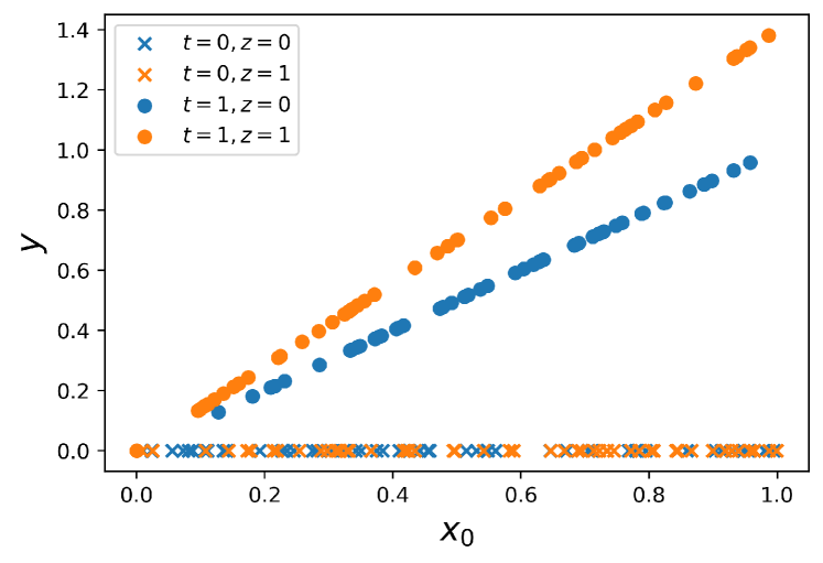
As proof of concept, we demonstrate our approach on synthetic data representing observations from a hypothetical experiment. The individual observations have features, , , drawn independently from a uniform distribution in range . The treatment assignment and sensitive feature are generated independently using Bernoulli distributions: . Finally, the observed outcomes depend on features and treatment as follows:
| (17) |
Note that the feature is designed to not correlate with .
Figure 1 shows the outcomes for the control () and treated () individuals. The two subgroups have the same outcome in the control case, but individuals from the protected subgroup () benefit more from the treatment (), since their outcomes are higher than for individuals from the other group (). Note that the larger the feature , the larger the impact of treatment on the protected subgroup . The disparate response to treatment creates a dilemma for decision makers—if both subgroups receive the same treatment (), then higher population-wide outcome will be associated with a larger discrepancy in the outcomes for the two subgroups, hence, larger bias ().
We train a causal tree to estimate the heterogeneous treatment effect using . Given total observations, we use a third of the data for training the causal tree, a third for validation, and a third for estimation using honest trees (athey-pnas16, ). We estimate biases for the sensitive attribute and learn optimal interventions using data reserved in the estimation set.
Equal Treatment Policy
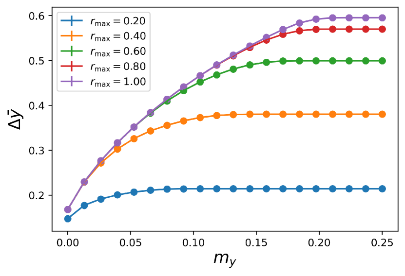
First we consider the equal treatment policy, where individuals from either subgroup are equally likely to be treated. As described in the preceding section, in this case . To model limited resources, such as limited doses of a vaccine or limited number of spots in the academic intervention program, we assume that we can only treat up to individuals. For simplicity, we introduce , which is the maximum treatment ratio as a measure of resource limit. Also we use
as a measure of the improvement of the outcome after treatment. We vary treatment ratio in , and for each value of plot the improvement in overall outcome of the intervention () as a function of , the upper limit of the bias in outcomes (). Figure 2(a) shows that as we treat more individuals (larger ), there is greater benefit from the intervention in terms of larger overall outcome (). Additionally, as we tolerate more bias ( increases), the overall outcome also increases. However, for large enough , there is no more benefit from the intervention. In this case, we have assigned all the necessary treatment and allowing more bias will not further improve the outcome. In other words, when no more people can be treated under the constraint , and is maximized.
Affirmative Action Policy
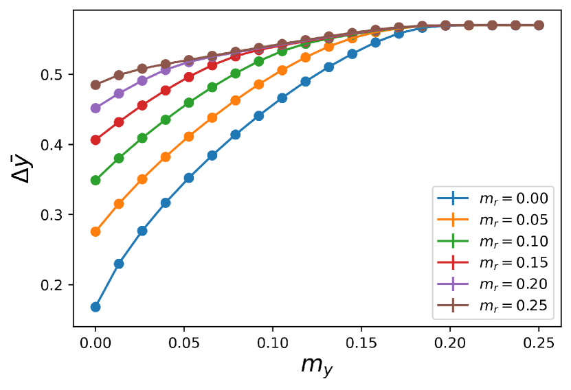
To see how affirmative action could improve the average overall outcome, we fix and vary in . This allows us to prioritize protected subgroups for treatment. As more individuals from protected subgroups are treated, the treatment ratios become different, increasing .
Figure 2(b) shows the overall outcome as a function of maximum bias for different values of . The curve is the degenerate case where the previous policy of equal opportunity holds. We see that at large , different curves of different values of reach the same upper bound of , which is constrained by . For lower values of , affirmative action dramatically increases , i.e., preferentially selecting individuals from protected subgroups for treatment increases the overall benefit of treatment.
Trade-offs between and
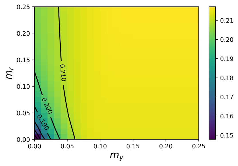
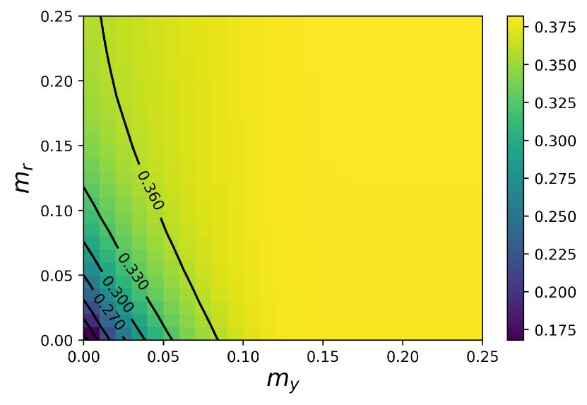
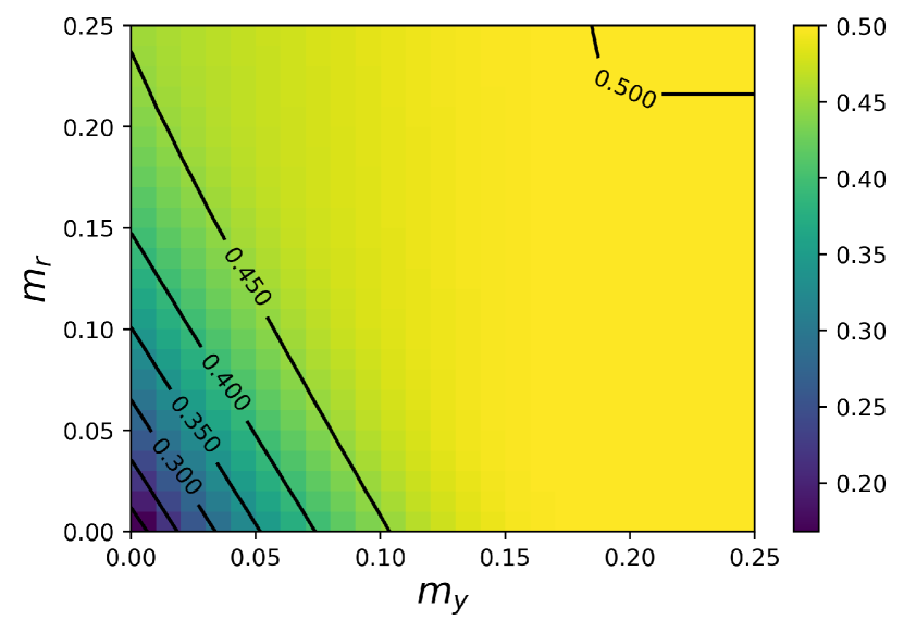
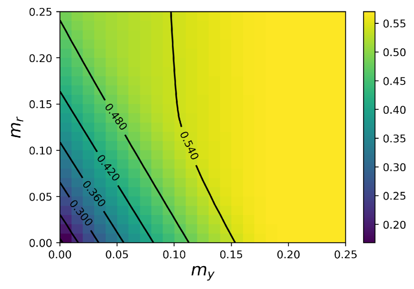
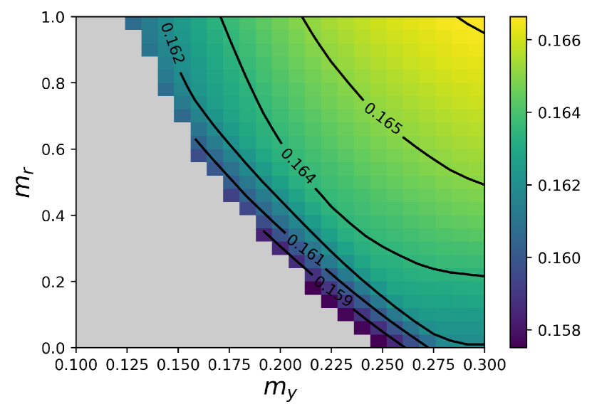
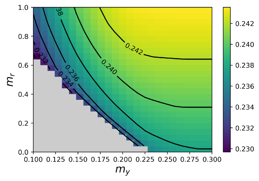
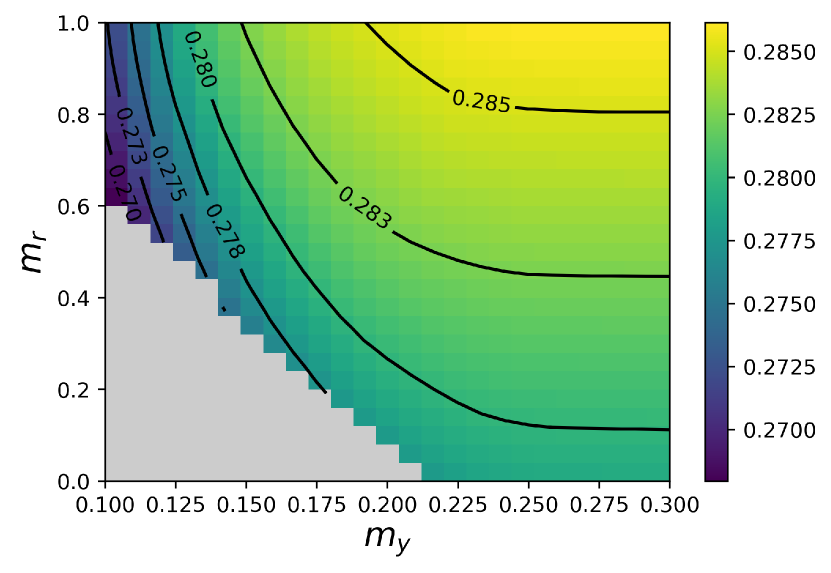
To further illustrate the how and affect the outcome , we plot against and using heat map and contour line, as shown in Fig. 3. The heatmap and contour lines demonstrates the trade-offs between the two biases. In order to maintain the same level of benefit from the intervention (moving along the contour lines) while reducing maximum allowed treatment opportunity bias requires us to tolerate larger treatment outcome bias and vice versa.
4.2. EdGap Data
The EdGap data contains education performance of different counties of United States. The data we used contains around 2000 counties and 19 features. The features include funding, normalized mean test score, average school size, number of magnet schools, number of charter schools, percent of students took standardized tests and average number of students in schools receiving discounted or free lunches. Besides these features, we have census features for each county including household mean income, household marriage ratio, Black household ratio, percent of people who finished high school, percent of people with a bachelor’s degree, employment ratio, and Gini coefficient. We use z-score normalized mean test score as the outcome. We binarize school funding and the county ratio of Black households to be above and below the median values as treatment indicator and sensitive feature, respectively. In summary, we are interested in the heterogeneous effect of funding increase on different counties and we want to design a fair intervention which reduces the education performance difference between Black and non-Black populations.
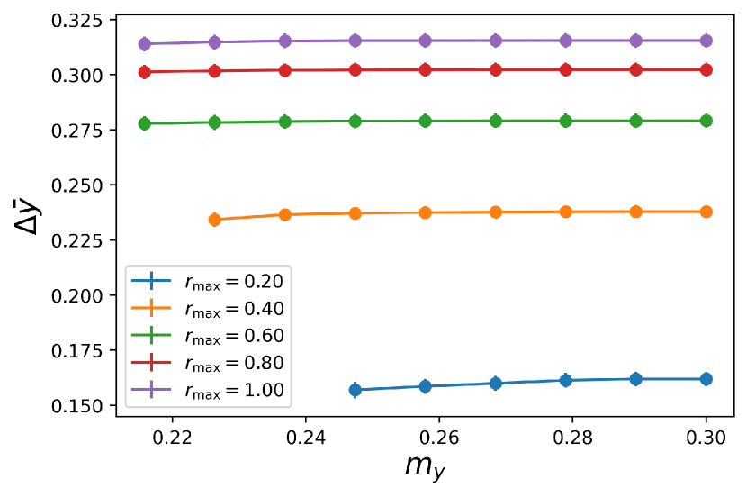
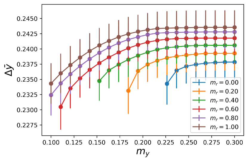
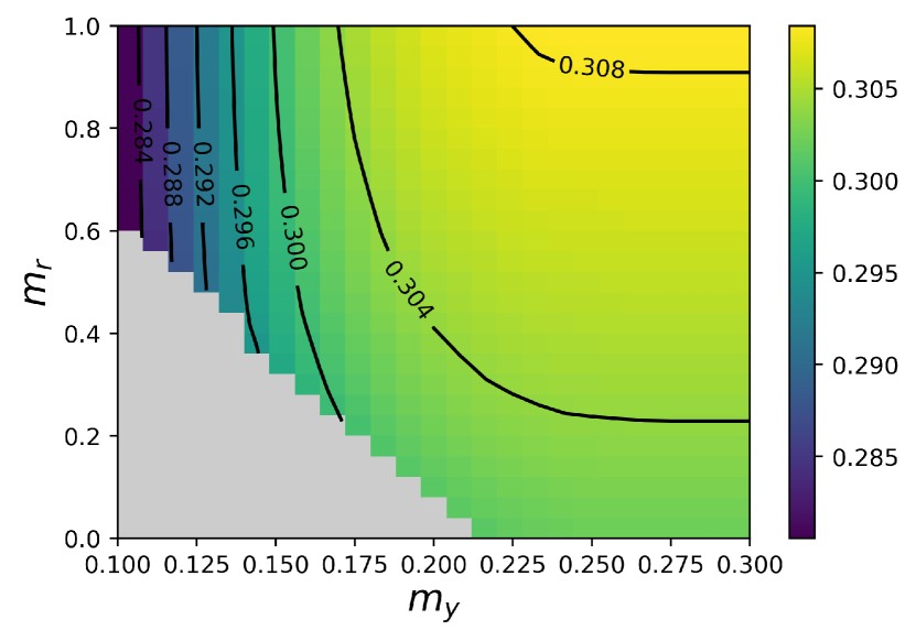
We use one third of data as training, validation and testing, respectively and train forty boosted causal trees and report the average performance. We first show the result where equal treatment opportunity is assumed. We plot the overall mean score after treatment versus in Fig.4(a). Unlike the synthetic data (Fig.2(a)), we find an infeasible region (note that the left bound of curves are different; beyond the left bound is the infeasible region). The lower the maximum allowed treatment ratio, the larger the infeasible region. This is because, without any treatment, there is a difference in the mean of average test scores for county with more Black population and less Black population. If the constrain , score difference between two groups of county, is set to be too low and the maximum allowed treatment ratio is also low, the constraints cannot be satisfied. But on the other hand, we also notice that if affirmative action is allowed, we can assign more counties with high Black ratio to treatment and dramatically improve the mean outcome and also reduce the infeasible region (allow greater fairness), as shown in Fig. 4(b). We also plot versus and for different in heat maps (Fig. 5). We observe that the size of infeasible region (grey region) is reduced as and increase.
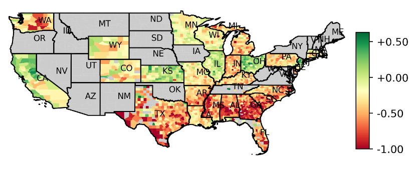
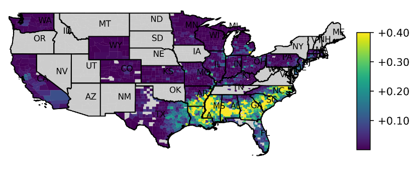
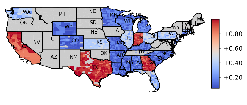
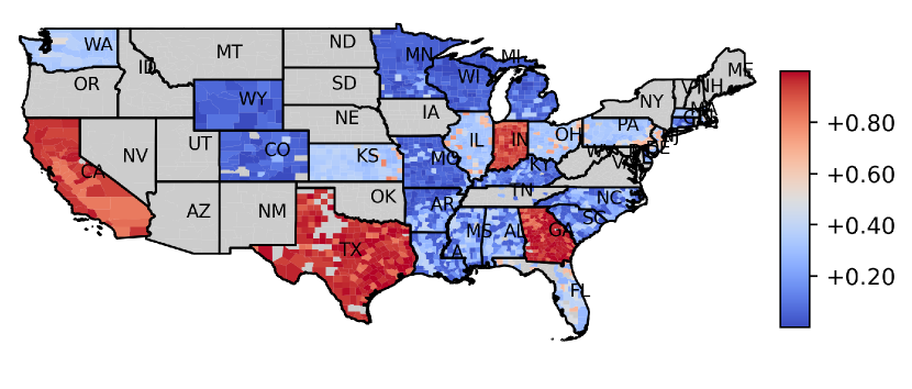
To further understand the bias in the data and the fair intervention we learned, we visualize the geographical distribution of data and the learned treatment assignment in Fig. 6. We first plot the mean test score of counties and the ratio of Black household in Fig. 6(a)–(b), respectively. We see that in the southeast states, from Louisiana to North Carolina, there are counties with high ratio of Black households. Correspondingly, we also see that the mean test scores of those counties are lower than national average due to chronic under-funding and racism. To illustrate the effect of affirmative action, we plot the learned optimal treatment assignments of two sets of parameters. First, we consider the case where we assume equal treatment opportunity. We use parameters , . Then for the case where affirmative action is allowed, we use parameters , . For both plots, we can see that counties in California, Texas, and Georgia have a high probability of being assigned to treatment. This is because the causal tree model predicts that counties in those state have higher treatment effect . Importantly, comparing Fig.6(c) and (d), we see when affirmative action is allowed, the counties in Louisiana, Mississippi, Alabama, South Carolina, and North Carolina have a high probability of being assigned to treatment. The treatment will not only improve the overall performance, but will also reduce performance difference between counties with high and low Black households.
5. Discussion
In this paper, we ask how we can learn intervention policies that both improve desired outcomes and increase equality in treatment across any number of protected classes. To do so, we first create novel metrics to quantify the fairness of any policy, and then create fairer policies based on two complimentary, but distinct, definitions of fairness. These findings demonstrate a trade-off between policies that maximize outcomes and fairness. Increasing the overall outcome can bring unintended unequal treatments between protected classes. That said, the ways to mitigate this unfair treatment has its own trade-off. Policies that provide equal treatment to all classes still provide substantial overall unequal treatment. Affirmative action policies, in contrast, provide greater overall fairness, but imply that subgroups must receive unequal treatment. Finally, we provide an algorithm that offers the best policies, conditional on the trade-offs policy-makers’ desire.
While this methodology offers substantial benefits to policy-makers, our work still has limitations. First, the algorithm and metrics are tailored to causal trees. While trees are highly interpretable, numerous other causal methods exist, and other algorithms need to be tailored to these other methods (wager-jasa17, ; athey-annals19, ; Kunze2019, ). Second, there is an open question of how Bayesian networks (pearl-book09, ), which model the pathways of causality, relate to algorithms that model heterogenous treatment effects. Future work must explore how fair policies created via causal models relate to potentially fair policies created by Bayesian networks.
6. Acknowledgements
This project has been funded, in part, by DARPA under contract HR00111990114.
References
- [1] Julia Angwin, Jeff Larson, Surya Mattu, and Lauren Kirchner. Machine bias. propublica. See https://www. propublica. org/article/machine-bias-risk-assessments-in-criminal-sentencing, 2016.
- [2] Susan Athey and Guido Imbens. Recursive partitioning for heterogeneous causal effects. Proceedings of the National Academy of Sciences, 2016.
- [3] Susan Athey, Julie Tibshirani, Stefan Wager, et al. Generalized random forests. The Annals of Statistics, 47(2):1148–1178, 2019.
- [4] Silvia Chiappa. Path-specific counterfactual fairness. In Proceedings of the AAAI Conference on Artificial Intelligence, volume 33, pages 7801–7808, 2019.
- [5] Alexandra Chouldechova, Diana Benavides-Prado, Oleksandr Fialko, and Rhema Vaithianathan. A case study of algorithm-assisted decision making in child maltreatment hotline screening decisions. In Conference on Fairness, Accountability and Transparency, pages 134–148, 2018.
- [6] Sam Corbett-Davies, Emma Pierson, Avi Feller, Sharad Goel, and Aziz Huq. Algorithmic decision making and the cost of fairness. In Proceedings of the 23rd acm sigkdd international conference on knowledge discovery and data mining, pages 797–806, 2017.
- [7] Kate Donahue and Jon Kleinberg. Fairness and utilization in allocating resources with uncertain demand. In Proceedings of the 2020 Conference on Fairness, Accountability, and Transparency, pages 658–668, 2020.
- [8] Hadi Elzayn, Shahin Jabbari, Christopher Jung, Michael Kearns, Seth Neel, Aaron Roth, and Zachary Schutzman. Fair algorithms for learning in allocation problems. In Proceedings of the Conference on Fairness, Accountability, and Transparency, pages 170–179, 2019.
- [9] Ezekiel J Emanuel, Govind Persad, Ross Upshur, Beatriz Thome, Michael Parker, Aaron Glickman, Cathy Zhang, Connor Boyle, Maxwell Smith, and James P Phillips. Fair allocation of scarce medical resources in the time of covid-19. N Engl J Med, pages 2049–2055, 2020.
- [10] James Foulds, Rashidul Islam, Kamrun Naher Keya, and Shimei Pan. An intersectional definition of fairness. arXiv preprint arXiv:1807.08362, 2019.
- [11] Aditya Grover, Kristy Choi, Rui Shu, and Stefano Ermon. Fair generative modeling via weak supervision. arXiv preprint arXiv:1910.12008, 2019.
- [12] Moritz Hardt, Eric Price, and Nathan Srebro. Equality of opportunity in supervised learning. In 30th Conference on Neural Information Processing Systems (NIPS 2016), Barcelona, Spain., pages 3323–3331, 2016.
- [13] Yuzi He, Keith Burghardt, and Kristina Lerman. A geometric solution to fair representations. In Proceedings of the AAAI/ACM Conference on AI, Ethics, and Society, pages 279–285, 2020.
- [14] Peter Kairouz, Jiachun Liao, Chong Huang, and Lalitha Sankar. Censored and fair universal representations using generative adversarial models. arXiv, pages arXiv–1910, 2019.
- [15] Jon Kleinberg, Sendhil Mullainathan, and Manish Raghavan. Inherent trade-offs in the fair determination of risk scores. arXiv preprint arXiv:1609.05807, 2016.
- [16] Sören R. Künzel, Jasjeet S. Sekhon, Peter J. Bickel, and Bin Yu. Metalearners for estimating heterogeneous treatment effects using machine learning. Proceedings of the National Academy of Sciences, 116(10):4156–4165, 2019.
- [17] Matt J Kusner, Joshua Loftus, Chris Russell, and Ricardo Silva. Counterfactual fairness. In Advances in neural information processing systems, pages 4066–4076, 2017.
- [18] Christos Louizos, Kevin Swersky, Yujia Li, Max Welling, and Richard Zemel. The variational fair autoencoder. arXiv preprint arXiv:1511.00830, 2015.
- [19] Aditya Krishna Menon and Robert C Williamson. The cost of fairness in binary classification. In Conference on Fairness, Accountability and Transparency, pages 107–118, 2018.
- [20] Daniel Moyer, Shuyang Gao, Rob Brekelmans, Aram Galstyan, and Greg Ver Steeg. Invariant representations without adversarial training. In Advances in Neural Information Processing Systems, pages 9084–9093, 2018.
- [21] Razieh Nabi, Daniel Malinsky, and Ilya Shpitser. Learning optimal fair policies. Proceedings of machine learning research, 97:4674, 2019.
- [22] Razieh Nabi and Ilya Shpitser. Fair inference on outcomes. In Proceedings of the AAAI Conference on Artificial Intelligence. AAAI Conference on Artificial Intelligence, volume 2018, page 1931. NIH Public Access, 2018.
- [23] Ziad Obermeyer, Brian Powers, Christine Vogeli, and Sendhil Mullainathan. Dissecting racial bias in an algorithm used to manage the health of populations. Science, 366(6464):447–453, 2019.
- [24] Judea Pearl. Causality. Cambridge university press, 2009.
- [25] Alvin Rajkomar, Michaela Hardt, Michael D Howell, Greg Corrado, and Marshall H Chin. Ensuring fairness in machine learning to advance health equity. Annals of internal medicine, 169(12):866–872, 2018.
- [26] S. Verma and J. Rubin. Fairness definitions explained. In 2018 IEEE/ACM International Workshop on Software Fairness (FairWare), pages 1–7, 2018.
- [27] Stefan Wager and Susan Athey. Estimation and inference of heterogeneous treatment effects using random forests. Journal of the American Statistical Association, 2017.
- [28] Yanyan Wang, Vicki M Bier, and Baiqing Sun. Measuring and achieving equity in multiperiod emergency material allocation. Risk Analysis, 39(11):2408–2426, 2019.
- [29] Depeng Xu, Shuhan Yuan, Lu Zhang, and Xintao Wu. Fairgan+: Achieving fair data generation and classification through generative adversarial nets. In 2019 IEEE International Conference on Big Data (Big Data), pages 1401–1406. IEEE, 2019.
- [30] Muhammad Bilal Zafar, Isabel Valera, Manuel Gomez Rodriguez, and Krishna P Gummadi. Fairness beyond disparate treatment & disparate impact: Learning classification without disparate mistreatment. In Proceedings of the 26th international conference on world wide web, pages 1171–1180, 2017.
- [31] Muhammad Bilal Zafar, Isabel Valera, Manuel Rodriguez, Krishna Gummadi, and Adrian Weller. From parity to preference-based notions of fairness in classification. In Advances in Neural Information Processing Systems, pages 229–239, 2017.
- [32] Muhammad Bilal Zafar, Isabel Valera, Manuel Gomez Rogriguez, and Krishna P Gummadi. Fairness constraints: Mechanisms for fair classification. In Artificial Intelligence and Statistics, pages 962–970. PMLR, 2017.
- [33] Lu Zhang, Yongkai Wu, and Xintao Wu. A causal framework for discovering and removing direct and indirect discrimination. arXiv preprint arXiv:1611.07509, 2016.