Deep Learning Ensemble for Real-time Gravitational Wave Detection
of Spinning Binary Black Hole Mergers

Abstract

We introduce the use of deep learning ensembles for real-time, gravitational wave detection of spinning binary black hole mergers. This analysis consists of training independent neural networks that simultaneously process strain data from multiple detectors. The output of these networks is then combined and processed to identify significant noise triggers. We have applied this methodology in O2 and O3 data finding that deep learning ensembles clearly identify binary black hole mergers in open source data available at the Gravitational-Wave Open Science Center. We have also benchmarked the performance of this new methodology by processing 200 hours of open source, advanced LIGO noise from August 2017. Our findings indicate that our approach identifies real gravitational wave sources in advanced LIGO data with a false positive rate of 1 misclassification for every 2.7 days of searched data. A follow up of these misclassifications identified them as glitches. Our deep learning ensemble represents the first class of neural network classifiers that are trained with millions of modeled waveforms that describe quasi-circular, spinning, non-precessing, binary black hole mergers. Once fully trained, our deep learning ensemble processes advanced LIGO strain data faster than real-time using 4 NVIDIA V100 GPUs.

I Introduction

The advanced LIGO The LIGO Scientific Collaboration et al. (2015) and Virgo Acernese et al. (2015) detectors have reported over fifty gravitational wave observations by the end of their third observing run Abbott et al. (2020a). Gravitational wave detection is now routine. It is then timely and necessary to accelerate the development and adoption of signal processing tools that minimize time-to-insight, and that optimize the use of available, oversubscribed computational resources.

Over the last decade, deep learning has emerged as a go-to tool to address computational grand challenges across disciplines. It is extensively documented that innovative deep learning applications in industry and technology have addressed big data challenges that are remarkably similar to those encountered in gravitational wave astrophysics. It is then worth harnessing these developments to help realize the science goals of gravitational wave astrophysics in the big data era.

The use of deep learning to enable real-time gravitational wave observations was first introduced in George and Huerta (2018a) in the context of simulated advanced LIGO noise, and then extended to real advanced LIGO noise in George et al. (2017); George and Huerta (2018b). Over the last few years this novel approach has been explored in earnest Gabbard et al. (2018); Skliris et al. (2020); Lin and Wu (2020); Wang et al. (2020); Nakano et al. (2019); Fan et al. (2019); Li et al. (2020); Deighan et al. (2020); Miller et al. (2019); Krastev (2020); Schäfer et al. (2020); Dreissigacker and Prix (2020); Khan et al. (2020); Dreissigacker et al. (2019); Beheshtipour and Papa (2020); Skliris et al. (2020); Khan and Green (2020); Chua et al. (2019); Wei and Huerta (2020). However, several challenges remain. To mention a few, deep learning detection algorithms continue to use shallow signal manifolds which typical involve only the masses of the binary components. There is also a pressing need to develop models that process long datasets in real-time while ensuring that they keep the number of misclassifications at a minimum. This article introduces the use of deep learning ensembles to address these specific issues.

We showcase the application of this approach by identifying all binary black hole mergers reported during advanced LIGO’s second and third observing runs. We also demonstrate that when we feed 200 hours of advanced LIGO data into our deep learning ensemble, this method is capable of clearly identifying real events, while also significantly reducing the number of misclassifications to just 1 for every 2.7 days of searched data. When we followed up these misclassifications, we realized that they were loud glitches in Livingston data.

I.1 Executive Summary

At a glance the main results of this article are:

• We introduce the first class of neural network classifiers that sample a 4-D signal manifold that describes quasi-circular, spinning, non-precessing binary black hole mergers.

• We use deep learning ensembles to search for and detect real binary black hole mergers in open source data from the second and third observing runs available at the Gravitational-Wave Open Science Center Vallisneri et al. (2015).

• Our deep learning ensemble is used to process 200 hours of open source advanced LIGO noise, finding that this methodology: (i) processes data faster than real-time using a single GPU; (ii) clearly identifies real events in this benchmark dataset; and (iii) reports only three misclassifications that are associated with loud glitches in Livingstone data.

This paper is organized as follows. Section II describes the architecture of the neural networks used to construct the ensemble. Section III summarizes the modeled waveforms and real advanced LIGO noise used to train the ensemble. We summarize our results in Section IV, and outline future directions of research in Section V.

II Neural Network Architecture

It is now well established that the design of a neural network architecture is as critical as the choice of optimization schemes Raissi et al. (2017a, b). Based on previous studies we have conducted to denoise real gravitational wave signals Wei and Huerta (2020), and to characterize the signal manifold of quasi-circular, spinning, non-precessing, binary black hole mergers Khan Asad, E. A. Huerta and Arnav Das (2020); Khan et al. (2020), we have selected WaveNet van den Oord et al. (2016) as the baseline architecture for gravitational wave detection. As we describe below, we have modified the original architecture with a number of important features tailored for signal detection.

II.1 Primary Architecture

WaveNet van den Oord et al. (2016) has been extensively used to process waveform-type time-series data, such as raw audio waveforms that mimic human speech with high fidelity. It is known to adapt well to time-series of high sample rate, as its dilated convolution layers allows larger reception fields with fewer parameters, and its blocked structure allows response to a combination of frequencies ranges.

Since we are using WaveNet for classification instead of waveform generation, we have removed the causal structure of the network described in van den Oord et al. (2016). The causal structure of WaveNet is modeled with a convolutional layer Krizhevsky et al. (2012) with kernel size 2, and by shifting the output of a normal convolution by a few time steps. However, in this paper we adopt convolutional layers with kernel size 3, so that the neural network will take into consideration both past and future information when deciding on the label at the current time step. We also dilate the convolutional layers to get an exponential increase in the size of the receptive field van den Oord et al. (2016). This is necessary to capture long-range correlations, as well as to increase computational efficiency. By construction, WaveNet utilizes deep residual learning, which is specifically tailored to train deeper neural network models He et al. (2016). The structure of WaveNet is described in detail in van den Oord et al. (2016). Below we describe tailored, WaveNet-based architectures for gravitational wave detection.

II.2 WaveNet Architecture I

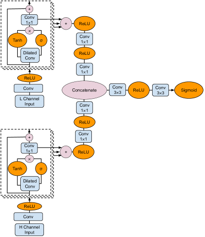
Model I processes Livingston and Hanford strain data using two independent WaveNet models. Then the output of the two WaveNets is concatenated, and fed into the last two convolutional layers. Finally, a sigmoid transformation is applied to ensure that the output values are in the range of $[0,1]$. The network structure is shown in Figure 1.

Figure 1: Architecture of our WaveNet detection algorithm. The input and output are tensors of shape $\textrm{batch\_size}\times 1\times\texttt{model}$, where $\texttt{model}=\{16384,\,4096\}$.

II.3 WaveNet Architecture II

Model II is essentially the same shown in Figure II.2, except that the input now consists of $1$s long strain data sampled at $4096$ Hz. Additionally, we reduce the depth of the model by cutting down to $4$ residual blocks, and reduce the number of filters, and revert back to kernel size $2$.

III Data Curation

In this section we describe the modeled waveforms used for training, and the strategy followed to combine these signals with real advanced LIGO noise.

III.1 Modeled Waveforms

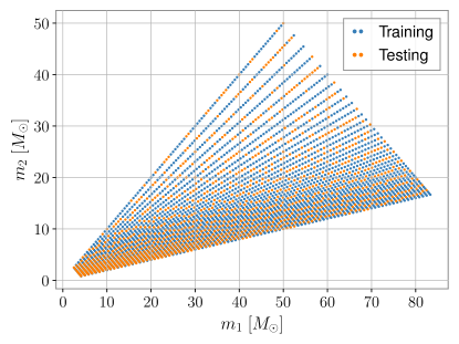
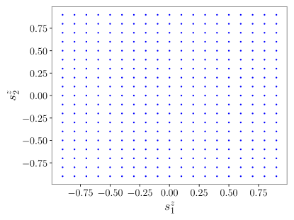
We train our neural networks using SEOBNRv3 waveforms Pan et al. (2014). Our datasets consist of time-series waveforms that describe the last second of evolution that includes the late inspiral, merger and ringdown of quasi-circular, spinning, non-precessing, binary black hole mergers. Each waveform is produced at a sample rate of 16384Hz and 4096Hz. The parameter space covered for training encompasses total masses $M\in[5{\rm M}_{\odot},\,100{\rm M}_{\odot}]$, mass-ratios $q\leq 5$, and individual spins $s^{z}_{\{1,2\}}\in[-0.8,\,0.8]$. The sampling of this 4-D parameter space is shown in Figure 2. It is worth pointing out that even though these models cover a total mass range $M\leq 100{\rm M}_{\odot}$, our models are able to generalize, since they can clearly identify the O3 event GW190521, which has an estimated total mass $M\sim 142{\rm M}_{\odot}$ Abbott et al. (2020b).

We consistently encode ground truth labels for waveforms in a binary manner, where data points before the amplitude peak of every waveform are labeled as 1, while the data points after the merger are labelled as 0. In other words, the change from 1’s to 0’s indicates the location of the merger.

Figure 2: Sampling of the component mass and individual spin parameter space $(m_{1},\,m_{2},\,s_{1}^{z},\,s_{2}^{z})$ for training and testing.

III.2 Advanced LIGO noise for training

We prepare the noise used for training by selecting continuous segments of advanced LIGO noise from the Gravitational Wave Open Science Center Vallisneri et al. (2015), which are typically 4096 seconds long. None of these segments include known gravitational wave detections. These data are used to compute noise power spectral density (PSD) estimates Usman et al. (2016) that are used to whiten both the strain data and the modeled waveforms. Thereafter, the whitened strain data and the whitened modeled waveforms are linearly combined, and a broad range of signal-to-noise ratios are covered to encode scale invariance in the neural network. We then normalize the standard deviation of training data that contain both signals and noise to one.

We also encode time-invariance into our training data, which is critical to correctly detect signals in arbitrarily long data stream irrespective of their locations. For every one second long segments with injections used for training, the injected waveform is located at a random location, with the only constraint that its peak must locate inside the second half of the 1s-long input time series. To improve the robustness of the trained model, only 40% of the samples in the training set contain GW signals, while the rest 60% samples are advanced LIGO noise only.

We present a more detailed description of the training approach for Model I and Model II below.

III.2.1 Training for Model I

Model I is trained on three 4096s-long data segments with starting GPS time $1186725888$, $1187151872$, and $1187569664$. After we whitened the three segments separately with the corresponding PSD, we truncated 122s-long data from each end of the segment to remove edge effects. The neural network trained this way is able to successfully detect the gravitational wave events GW170104, GW170729, GW170809, GW170814, GW170817, GW170818, GW170823, GW190412.

This neural network is also able to detected GW170608 and GW190521 after further trained on advanced LIGO data close to these two events. Specifically, to detect GW170608, the neural network is further trained on two 4096s-long data segments with starting GPS time $1178181632$, and $1180983296$. Similarly, to detect GW190521, the neural network is further trained on the 2048s-long data segments around GW190521.

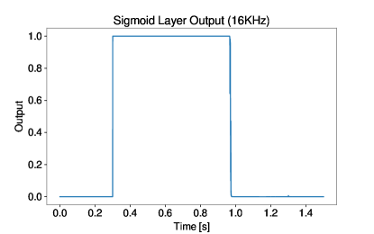
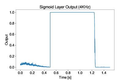
The input to the neural network is a 1s-long $16384$Hz data segment, with two channels from Livingston and Hanford observatories. The output of the neural network has one channel and is of the same length as the input. The output is $1$ when there is signal at the corresponding location in the input, and $0$ otherwise.

To ensure that signals contaminated by advanced LIGO noise generate long enough responses, we make sure that the flat peak of the neural network output is located in the second half of the 1s-long input. In other words, when there is a signal in the second half of the 1s-long input, the ground-truth output would be a peak of width of at least $8192$. Furthermore, to ensure that all possible signal peaks appear in the second half of the input data segment, we feed the test data into the neural network with a step size of $8192$, i.e., we crop out 1s-long data segment of size $16384$ every $8192$ data points.

To constrain the output of the neural network in the range $[0,1]$, we apply the sigmoid function $s(x)=1/(1+\exp(-x))$ element-wise on the final output from neural network, as shown in Figure 1. We use the binary cross entropy loss to evaluate the prediction of the neural network when compared to ground-truth values. Finally, to avoid possible overfitting, we augment the training data by reversing the 1s-long data segments in the time dimension with a probability of $0.5$.

III.2.2 Training for Model II

Model II did not require fine-tuning on advanced LIGO data around any specific events, i.e., it was able to detect all O2 and O3 events after the initial round of training which, as mentioned above, consisted of three 4096s-long data segments with starting GPS time $1186725888$, $1187151872$, and $1187569664$. Furthermore, data augmentation of training data by randomly reversing the 1s long input strains was not employed.

Figure 3: Post-processing output of Model I, left panel, and Model II, right panel, for the event GW170809. Notice that we have zoomed in to show the neural network response in the vicinity of the waveform signal.

III.3 Optimization Methodology

Model I The neural networks are trained on 4 NVIDIA K80 GPUs in the Bridges-AI system XSEDE , and also on 4 NVIDIA V100 GPUs in the Hardware Accelerated Learning (HAL) deep learning cluster NCSA , with PyTorch Paszke et al. (2017). We use ADAM  Kingma and Ba (2014) optimization, and binary cross entropy as the loss function. The weight parameters are initialized randomly. The learning rate is set to $10^{-4}$.

Model II Model II is trained on 8 NVIDIA V100 GPUs in the HAL cluster NCSA with Tensorflow Abadi et al. (2016), once again using ADAM Kingma and Ba (2014) optimizer with binary cross entropy as the loss function. Similarly, the weights are initialized randomly, the initial learning rate is set to $10^{-4}$, and a step-wise learning rate scheduler is employed to attempt a more fine-grained convergence to a minima of the loss function.

III.4 Post-processing

Once the models process advanced LIGO strain data, their outputs are post-processed as follows.

III.4.1 Post-processing for Model I

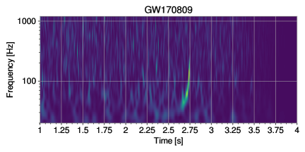
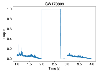
In the training set, for all input samples with gravitational waves, their labels will always have 1’s before the merger and 0’s after the merger, and because we always place the merger in the second half of the input time series, the length of the 1’s will be at least 8192. Therefore, if the input 1s-long data strain contains a gravitational wave, the output of the neural network would be a peak with a height of 1 and a width of at least $8192$. Based on this setup, the output of the neural network will be further fed into the off-the-shelf peak detection algorithm find_peaks provided by SciPy. The algorithm will then output the locations of possible peaks that satisfy the conditions of at least $0.9995$ in height and $8192$ in width. To avoid possible overcounting, we also assume that there is at most one signal in a 5s-long window. Furthermore, since a GW signal will induce a flat (all 1’s) and wide (at least 8192 in length) peak in the neural network output, we also use an additional criterion that 94% of the outputs between the left and right boundaries of the detected peak be greater than 0.99 to further reduce the false alarms. To showcase the application of this approach for real events, the left panel of Figure 3 presents the output of Model I for the event GW170809.

III.4.2 Post-processing for Model II

In the post-processing, the conditions for find_peaks algorithm were changed to $0.99993$ and $2048$ for height and width respectively. Also, the additional criterion was relaxed so that only 95% of the outputs between the left and right boundaries of the detected peak be greater than 0.95. The right panel of Figure 3 presents the post-processing output of Model II for the event GW170809.

III.4.3 Post-processing of deep learning ensemble

Finally, we combine the output of the deep learning models to identify noise triggers that pass a given threshold of detectability for each model. We do this by comparing the GPS times for all triggers between each model. By definition (in the separate post-processing for each model), each model can only produce at most one trigger every 5 seconds. Hence, when combining the triggers from the two models, any triggers more than 5 seconds apart can be dropped as random False Alarms. In fact, since each model is extremely precise at identifying the merger location, we apply a much stricter criterion, namely, i.e., any triggers more than $1/128$ seconds apart between the two models are dropped as False Alarms, whereas triggers within $1/128$ seconds of each other are counted as a single Positive Detection.

In the following section we use this approach to search for gravitational waves in minutes, hours, and hundreds of hours long real advanced LIGO data.

IV Results

Figure 4: Detection output of our deep learning ensemble for GW170104, top left; GW170818, top right; GW190412, bottom left; and GW190521, bottom right. Notice that our ensemble identifies all these events with no false positives in minutes and hour-long datasets.

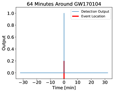
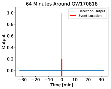
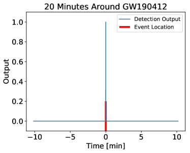
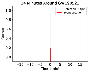
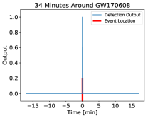
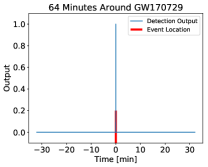
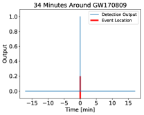
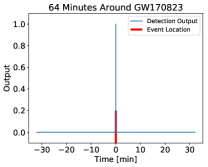
In this section we present results for the performance of our deep learning ensemble to search for and detect binary black hole mergers in O2 and O3 data. These results are summarized in Figures 4, and Figure 7 in Appendix A.

Figure 4 shows that our deep learning ensemble can detect O2 and O3 events without any additional false positives in the minutes or hour-long datasets released at the Gravitational-Wave Open Science Center containing these events. Similar results may be found in Figure 7 in Appendix A. To the best of our knowledge this is the first time deep learning is used to search for and detect real events, while also reducing the number of false positives at this level, in hours-long datasets. Notice also that our method can generalize to detect events that are beyond the parameter space used to train our neural networks. This is confirmed by the detection of GW190521, bottom right panel in Figure 4, which has an estimated total mass $M\sim 142{\rm M}_{\odot}$, whereas our training dataset covered systems with total mass $M\leq 100{\rm M}_{\odot}$.

While this is a significant result, it is also essential to benchmark the performance of our approach using much longer datasets. We have done this by processing 200hrs of advanced LIGO noise from August 2017. We feed these data into our deep learning ensemble to address two issues: (i) the sensitivity of the ensemble to real events in long datasets; and (ii) quantify the number of false positives, and explore the nature of false positives to gain additional insights into the response of our deep learning ensemble to both signals and noise anomalies. The results of this analysis are presented in Figure 5.

Figure 5: Output of our deep learning ensemble upon processing Livingston and Hanford data between August 5-16, 2017. This methodology identifies the two real events contained therein, while also indicating the existence of three false positives, associated to loud glitches in the Livingston channel. Every tick represents a day. These data were processed within 14 hours using 4 NVIDIA V100 GPUs.

At a glance, Figure 5 indicates that our approach identifies two real events contained in this 200hr-long dataset, namely, GW170809 and GW170814. These two events are marked with red lines in Figure 5. We also notice that our ensemble indicates the existence of three additional noise triggers, marked by blue and yellow lines, which are worth following up.

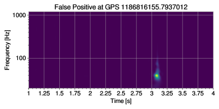
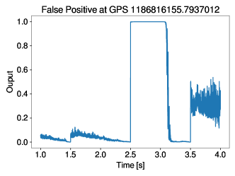
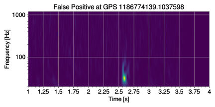
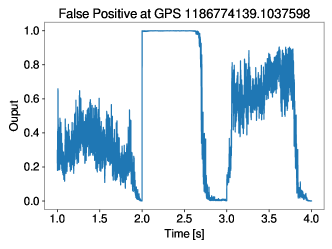
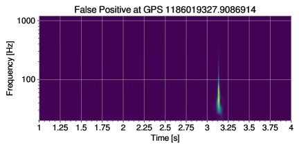
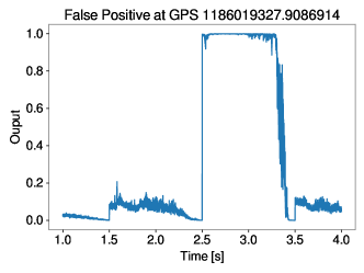
We have looked into these three noise triggers to figure out why they were singled out by our deep learning ensemble. We present spectrograms and the response of Model II to these events in Figure 6. As shown in the left panels of this figure, all three false positives are caused by loud glitches in Livingston data. Another interesting result we observe in these panels is that the response of our deep learning models to these false positives is different to real events, as shown in the bottom panels of Figure 6; see also Figure 3. Note that the response of our neural networks for real events is sharp-edged, whereas the neural networks’ response to noise anomalies is, at best, jagged. This is an additional feature that may be used to tell apart real events from other noise anomalies.

Figure 6: Left panel: normalized L–channel spectrograms around three false positives and GW170809. Right panel: as left panel, but now for the detection output of Model II.

In summary, we have designed a deep learning ensemble that can identify binary black hole mergers in O2 and O3 data. Our benchmark analyses indicate that our ensemble can process 200 hrs of advanced LIGO noise within 14 hours using one node in the HAL cluster, which consists of 4 NVIDIA V100 GPUs. We have found that this approach identifies real events in advanced LIGO data, and produces 1 misclassification for every 2.7 days of searched data. We have also found that our ensemble can generalize to astrophysical signals whose parameters are beyond the parameter space used for training, which furnishes evidence for the ability of our models to generalize to new signals.

This new method lays the foundation for the design of a production scale deep learning pipeline for gravitational wave searches, which we will present in an upcoming publication.

V Conclusions

We have introduced neural networks that cover a 4-D signal manifold that describe quasi-circular, spinning, non-precessing binary black hole mergers. We have shown that the use of deep learning ensembles enables the detection of O2 and O3 binary black hole mergers. We have also demonstrated that when this method is applied to hundreds of hours of advanced LIGO noise, we can identify real events contained in these data nearly ten times faster than real-time, with the additional advantage of reducing the number of false positives to about one for every 2.7 days of searched data.

Future work will build upon this framework, enlarging the parameter space so as to cover a wider range of astrophysical sources that are detectable by advanced ground-based detectors, including binary neutron stars and neutron star-black hole mergers, the latter being enhanced by early warning detection methods Wei and Huerta (2020).

As data associated with new gravitational wave detections become available through the Gravitational-Wave Open Science Center, it will be feasible to better tune detection thresholds in these models, which at this point are experimental in nature. It may also be possible to start using real events for training purposes, which will increase the sensitivity of deep learning searches. In brief, deep learning methods are at a tipping point of enabling accelerated gravitational wave detection searches.

Appendix A Additional O2 and O3 binary black hole mergers

We present the output of our deep learning ensemble for O2 and O3 binary black hole merger detections—see Figure 7. Note that as we discussed in the main body of the article, our approach identifies these events, and produces no false positives over the minutes and hour-long datasets containing these real events.

Figure 7: Detection output of our deep learning ensemble for GW170608, top left; GW170729, top right; GW170809, middle left; GW170814, middle right; and GW170823, bottom panel. Notice that our ensemble identifies all these events with no false positives in minutes and hour-long datasets.

References

- The LIGO Scientific Collaboration et al. (2015) The LIGO Scientific Collaboration, J. Aasi, et al., Classical and Quantum Gravity 32, 074001 (2015), arXiv:1411.4547 [gr-qc] .
- Acernese et al. (2015) F. Acernese et al., Classical and Quantum Gravity 32, 024001 (2015).
- Abbott et al. (2020a) R. Abbott et al., (2020a), arXiv:2010.14527 [gr-qc] .
- George and Huerta (2018a) D. George and E. A. Huerta, Phys. Rev. D 97, 044039 (2018a), arXiv:1701.00008 [astro-ph.IM] .
- George et al. (2017) D. George, H. Shen, and E. Huerta, in NiPS Summer School 2017 (2017) arXiv:1711.07468 [astro-ph.IM] .
- George and Huerta (2018b) D. George and E. Huerta, Physics Letters B 778, 64 (2018b).
- Gabbard et al. (2018) H. Gabbard, M. Williams, F. Hayes, and C. Messenger, Physical Review Letters 120, 141103 (2018), arXiv:1712.06041 [astro-ph.IM] .
- Skliris et al. (2020) V. Skliris, M. R. Norman, and P. J. Sutton, arXiv preprint arXiv:2009.14611 (2020).
- Lin and Wu (2020) Y.-C. Lin and J.-H. P. Wu, arXiv preprint arXiv:2007.04176 (2020).
- Wang et al. (2020) H. Wang, S. Wu, Z. Cao, X. Liu, and J.-Y. Zhu, Phys. Rev. D 101, 104003 (2020), arXiv:1909.13442 [astro-ph.IM] .
- Nakano et al. (2019) H. Nakano, T. Narikawa, K.-i. Oohara, K. Sakai, H.-a. Shinkai, H. Takahashi, T. Tanaka, N. Uchikata, S. Yamamoto, and T. S. Yamamoto, Phys. Rev. D 99, 124032 (2019), arXiv:1811.06443 [gr-qc] .
- Fan et al. (2019) X. Fan, J. Li, X. Li, Y. Zhong, and J. Cao, Sci. China Phys. Mech. Astron. 62, 969512 (2019), arXiv:1811.01380 [astro-ph.IM] .
- Li et al. (2020) X.-R. Li, G. Babu, W.-L. Yu, and X.-L. Fan, Front. Phys. (Beijing) 15, 54501 (2020), arXiv:1712.00356 [astro-ph.IM] .
- Deighan et al. (2020) D. S. Deighan, S. E. Field, C. D. Capano, and G. Khanna, (2020), arXiv:2010.04340 [gr-qc] .
- Miller et al. (2019) A. L. Miller et al., Phys. Rev. D 100, 062005 (2019), arXiv:1909.02262 [astro-ph.IM] .
- Krastev (2020) P. G. Krastev, Phys. Lett. B 803, 135330 (2020), arXiv:1908.03151 [astro-ph.IM] .
- Schäfer et al. (2020) M. B. Schäfer, F. Ohme, and A. H. Nitz, Phys. Rev. D 102, 063015 (2020), arXiv:2006.01509 [astro-ph.HE] .
- Dreissigacker and Prix (2020) C. Dreissigacker and R. Prix, Phys. Rev. D 102, 022005 (2020), arXiv:2005.04140 [gr-qc] .
- Khan et al. (2020) A. Khan, E. Huerta, and A. Das, Phys. Lett. B 808, 0370 (2020), arXiv:2004.09524 [gr-qc] .
- Dreissigacker et al. (2019) C. Dreissigacker, R. Sharma, C. Messenger, R. Zhao, and R. Prix, Phys. Rev. D 100, 044009 (2019), arXiv:1904.13291 [gr-qc] .
- Beheshtipour and Papa (2020) B. Beheshtipour and M. A. Papa, Phys. Rev. D 101, 064009 (2020), arXiv:2001.03116 [gr-qc] .
- Skliris et al. (2020) V. Skliris, M. R. K. Norman, and P. J. Sutton, arXiv e-prints , arXiv:2009.14611 (2020), arXiv:2009.14611 [astro-ph.IM] .
- Khan and Green (2020) S. Khan and R. Green, arXiv preprint arXiv:2008.12932 (2020).
- Chua et al. (2019) A. J. K. Chua, C. R. Galley, and M. Vallisneri, Phys. Rev. Lett. 122, 211101 (2019).
- Wei and Huerta (2020) W. Wei and E. A. Huerta, arXiv e-prints , arXiv:2010.09751 (2020), arXiv:2010.09751 [gr-qc] .
- Vallisneri et al. (2015) M. Vallisneri, J. Kanner, R. Williams, A. Weinstein, and B. Stephens, Proceedings, 10th International LISA Symposium: Gainesville, Florida, USA, May 18-23, 2014, J. Phys. Conf. Ser. 610, 012021 (2015), arXiv:1410.4839 [gr-qc] .
- Raissi et al. (2017a) M. Raissi, P. Perdikaris, and G. E. Karniadakis, arXiv e-prints , arXiv:1711.10561 (2017a), arXiv:1711.10561 [cs.AI] .
- Raissi et al. (2017b) M. Raissi, P. Perdikaris, and G. E. Karniadakis, arXiv e-prints , arXiv:1711.10566 (2017b), arXiv:1711.10566 [cs.AI] .
- Wei and Huerta (2020) W. Wei and E. A. Huerta, Phys. Lett. B800, 135081 (2020), arXiv:1901.00869 [gr-qc] .
- Khan Asad, E. A. Huerta and Arnav Das (2020) Khan Asad, E. A. Huerta and Arnav Das, “A deep learning model to characterize the signal manifold of quasi-circular, spinning, non-precessing binary black hole mergers,” (2020), https://doi.org/10.26311/8wnt-3343.
- van den Oord et al. (2016) A. van den Oord, S. Dieleman, H. Zen, K. Simonyan, O. Vinyals, A. Graves, N. Kalchbrenner, A. Senior, and K. Kavukcuoglu, arXiv e-prints , arXiv:1609.03499 (2016), arXiv:1609.03499 [cs.SD] .
- Krizhevsky et al. (2012) A. Krizhevsky, I. Sutskever, and G. E. Hinton, in Advances in neural information processing systems (2012) pp. 1097–1105.
- van den Oord et al. (2016) A. van den Oord, S. Dieleman, H. Zen, K. Simonyan, O. Vinyals, A. Graves, N. Kalchbrenner, A. Senior, and K. Kavukcuoglu, “Wavenet: A generative model for raw audio,” (2016), arXiv:1609.03499 [cs.SD] .
- He et al. (2016) K. He, X. Zhang, S. Ren, and J. Sun, in Proceedings of the IEEE conference on computer vision and pattern recognition (2016) pp. 770–778.
- Pan et al. (2014) Y. Pan, A. Buonanno, A. Taracchini, L. E. Kidder, A. H. Mroué, H. P. Pfeiffer, M. A. Scheel, and B. Szilágyi, Phys. Rev. D 89, 084006 (2014), arXiv:1307.6232 [gr-qc] .
- Abbott et al. (2020b) R. Abbott et al. (LIGO Scientific, Virgo), Phys. Rev. Lett. 125, 101102 (2020b), arXiv:2009.01075 [gr-qc] .
- Usman et al. (2016) S. A. Usman et al., Classical and Quantum Gravity 33, 215004 (2016), arXiv:1508.02357 [gr-qc] .
- (38) XSEDE, “Bridges-AI,” https://portal.xsede.org/psc-bridges.
- (39) NCSA, “HAL Cluster,” https://wiki.ncsa.illinois.edu/display/ISL20/HAL+cluster.
- Paszke et al. (2017) A. Paszke, S. Gross, S. Chintala, G. Chanan, E. Yang, Z. DeVito, Z. Lin, A. Desmaison, L. Antiga, and A. Lerer, (2017).
- Kingma and Ba (2014) D. P. Kingma and J. Ba, arXiv preprint arXiv:1412.6980 (2014).
- Abadi et al. (2016) M. Abadi, P. Barham, J. Chen, Z. Chen, A. Davis, J. Dean, M. Devin, S. Ghemawat, G. Irving, M. Isard, M. Kudlur, J. Levenberg, R. Monga, S. Moore, D. G. Murray, B. Steiner, P. Tucker, V. Vasudevan, P. Warden, M. Wicke, Y. Yu, and X. Zheng, in Proceedings of the 12th USENIX Conference on Operating Systems Design and Implementation, OSDI’16 (USENIX Association, 2016) pp. 265–283.