Population properties of compact objects from the second LIGO–Virgo Gravitational-Wave Transient Catalog
Abstract
We report on the population of the 47 compact binary mergers detected with a false-alarm rate < in the second LIGO–Virgo Gravitational-Wave Transient Catalog, GWTC-2. We observe several characteristics of the merging binary black hole (BBH) population not discernible until now. First, the primary mass spectrum contains structure beyond a power-law with a sharp high-mass cut-off; it is more consistent with a broken power law with a break at , or a power law with a Gaussian feature peaking at (90% credible interval). While the primary mass distribution must extend to or beyond, only of systems have primary masses greater than . Second, we find that a fraction of BBH systems have component spins misaligned with the orbital angular momentum, giving rise to precession of the orbital plane. Moreover, % to % of BBH systems have spins tilted by more than , giving rise to a negative effective inspiral spin parameter . Third, we estimate merger rates, finding for BBH and for binary neutron stars. We find that the BBH rate likely increases with redshift ( credibility), but not faster than the star-formation rate ( credibility). Additionally, we examine recent exceptional events in the context of our population models, finding that the asymmetric masses of GW190412 and the high component masses of GW190521 are consistent with our models, but the low secondary mass of GW190814 makes it an outlier.
=3000
1 Introduction
We analyze the population properties of black holes (BHs) and neutron stars (NSs) in compact binary systems using data from the LIGO–Virgo Gravitational-wave Transient Catalog 2 (GWTC-2; Abbott et al., 2020c). The GWTC-2 catalog combines observations from the first two observing runs (O1 and O2; Abbott et al., 2019b) and the first half of the third observing run (O3a; Abbott et al., 2020c) of the Advanced LIGO (Aasi et al., 2015) and Advanced Virgo (Acernese et al., 2015) gravitational-wave observatories. With the additional candidates from O3a, we have more than quadrupled the number of events from O1 and O2, published in the first LIGO–Virgo Transient Catalog (GWTC-1; Abbott et al., 2019b). Counting only events with false alarm rate (FAR) (as opposed to the less conservative FAR threshold of in GWTC-2), the new combined catalog includes: two binary NS (BNS) events, 44 confident binary black hole (BBH) events, and one NS–BH (NSBH) candidate, which may be a BBH—a topic we discuss below. These 47 events are listed in Table 1. Our chosen FAR threshold ensures a relatively pure sample with only noise event (see Section 2) and excludes three marginal triggers presented in GWTC-2. Two of these excluded events are BBH candidates (\IfEqCaseGW190719AGW190413AGW190413_052954GW190719AGW190719_215514GW190620AGW190620_030421GW190514AGW190514_065416GW190731AGW190731_140936GW190503AGW190503_185404GW190602AGW190602_175927GW190929AGW190929_012149GW190517AGW190517_055101GW190915AGW190915_235702GW190425AGW190425GW190512AGW190512_180714GW190630AGW190630_185205GW190521AGW190521GW190413BGW190413_134308GW190924AGW190924_021846GW190930AGW190930_133541GW190706AGW190706_222641GW190408AGW190408_181802GW190909AGW190909_114149GW190728AGW190728_064510GW190426AGW190426_152155GW190412AGW190412GW190720AGW190720_000836GW190521BGW190521_074359GW190910AGW190910_112807GW190803AGW190803_022701GW190519AGW190519_153544GW190708AGW190708_232457GW190527AGW190527_092055GW190513AGW190513_205428GW190424AGW190424_180648GW190727AGW190727_060333GW190814AGW190814GW190707AGW190707_093326GW190828AGW190828_063405GW190828BGW190828_065509GW190701AGW190701_203306GW190421AGW190421_213856 and \IfEqCaseGW190909AGW190413AGW190413_052954GW190719AGW190719_215514GW190620AGW190620_030421GW190514AGW190514_065416GW190731AGW190731_140936GW190503AGW190503_185404GW190602AGW190602_175927GW190929AGW190929_012149GW190517AGW190517_055101GW190915AGW190915_235702GW190425AGW190425GW190512AGW190512_180714GW190630AGW190630_185205GW190521AGW190521GW190413BGW190413_134308GW190924AGW190924_021846GW190930AGW190930_133541GW190706AGW190706_222641GW190408AGW190408_181802GW190909AGW190909_114149GW190728AGW190728_064510GW190426AGW190426_152155GW190412AGW190412GW190720AGW190720_000836GW190521BGW190521_074359GW190910AGW190910_112807GW190803AGW190803_022701GW190519AGW190519_153544GW190708AGW190708_232457GW190527AGW190527_092055GW190513AGW190513_205428GW190424AGW190424_180648GW190727AGW190727_060333GW190814AGW190814GW190707AGW190707_093326GW190828AGW190828_063405GW190828BGW190828_065509GW190701AGW190701_203306GW190421AGW190421_213856) and one is an NSBH candidate (\IfEqCaseGW190426AGW190413AGW190413_052954GW190719AGW190719_215514GW190620AGW190620_030421GW190514AGW190514_065416GW190731AGW190731_140936GW190503AGW190503_185404GW190602AGW190602_175927GW190929AGW190929_012149GW190517AGW190517_055101GW190915AGW190915_235702GW190425AGW190425GW190512AGW190512_180714GW190630AGW190630_185205GW190521AGW190521GW190413BGW190413_134308GW190924AGW190924_021846GW190930AGW190930_133541GW190706AGW190706_222641GW190408AGW190408_181802GW190909AGW190909_114149GW190728AGW190728_064510GW190426AGW190426_152155GW190412AGW190412GW190720AGW190720_000836GW190521BGW190521_074359GW190910AGW190910_112807GW190803AGW190803_022701GW190519AGW190519_153544GW190708AGW190708_232457GW190527AGW190527_092055GW190513AGW190513_205428GW190424AGW190424_180648GW190727AGW190727_060333GW190814AGW190814GW190707AGW190707_093326GW190828AGW190828_063405GW190828BGW190828_065509GW190701AGW190701_203306GW190421AGW190421_213856).
The latest observations include a number of individually remarkable events, which invite theoretical speculation while providing challenges to existing models. The observation of high-mass binaries such as \IfEqCaseGW190521AGW190413AGW190413_052954GW190719AGW190719_215514GW190620AGW190620_030421GW190514AGW190514_065416GW190731AGW190731_140936GW190503AGW190503_185404GW190602AGW190602_175927GW190929AGW190929_012149GW190517AGW190517_055101GW190915AGW190915_235702GW190425AGW190425GW190512AGW190512_180714GW190630AGW190630_185205GW190521AGW190521GW190413BGW190413_134308GW190924AGW190924_021846GW190930AGW190930_133541GW190706AGW190706_222641GW190408AGW190408_181802GW190909AGW190909_114149GW190728AGW190728_064510GW190426AGW190426_152155GW190412AGW190412GW190720AGW190720_000836GW190521BGW190521_074359GW190910AGW190910_112807GW190803AGW190803_022701GW190519AGW190519_153544GW190708AGW190708_232457GW190527AGW190527_092055GW190513AGW190513_205428GW190424AGW190424_180648GW190727AGW190727_060333GW190814AGW190814GW190707AGW190707_093326GW190828AGW190828_063405GW190828BGW190828_065509GW190701AGW190701_203306GW190421AGW190421_213856 (Abbott et al., 2020e), which has a primary mass , is in tension with the sharp mass cutoff inferred from the GWTC-1 detections, forcing us to reconsider models for the distribution of black hole (BH) masses in binary systems (Abbott et al., 2020e, f). Here and in the following, the primary mass refers to the bigger of the two component masses in the binary, while the secondary mass refers to the smaller of the two. Along with \IfEqCaseGW190521AGW190413AGW190413_052954GW190719AGW190719_215514GW190620AGW190620_030421GW190514AGW190514_065416GW190731AGW190731_140936GW190503AGW190503_185404GW190602AGW190602_175927GW190929AGW190929_012149GW190517AGW190517_055101GW190915AGW190915_235702GW190425AGW190425GW190512AGW190512_180714GW190630AGW190630_185205GW190521AGW190521GW190413BGW190413_134308GW190924AGW190924_021846GW190930AGW190930_133541GW190706AGW190706_222641GW190408AGW190408_181802GW190909AGW190909_114149GW190728AGW190728_064510GW190426AGW190426_152155GW190412AGW190412GW190720AGW190720_000836GW190521BGW190521_074359GW190910AGW190910_112807GW190803AGW190803_022701GW190519AGW190519_153544GW190708AGW190708_232457GW190527AGW190527_092055GW190513AGW190513_205428GW190424AGW190424_180648GW190727AGW190727_060333GW190814AGW190814GW190707AGW190707_093326GW190828AGW190828_063405GW190828BGW190828_065509GW190701AGW190701_203306GW190421AGW190421_213856, \IfEqCaseGW190602AGW190413AGW190413_052954GW190719AGW190719_215514GW190620AGW190620_030421GW190514AGW190514_065416GW190731AGW190731_140936GW190503AGW190503_185404GW190602AGW190602_175927GW190929AGW190929_012149GW190517AGW190517_055101GW190915AGW190915_235702GW190425AGW190425GW190512AGW190512_180714GW190630AGW190630_185205GW190521AGW190521GW190413BGW190413_134308GW190924AGW190924_021846GW190930AGW190930_133541GW190706AGW190706_222641GW190408AGW190408_181802GW190909AGW190909_114149GW190728AGW190728_064510GW190426AGW190426_152155GW190412AGW190412GW190720AGW190720_000836GW190521BGW190521_074359GW190910AGW190910_112807GW190803AGW190803_022701GW190519AGW190519_153544GW190708AGW190708_232457GW190527AGW190527_092055GW190513AGW190513_205428GW190424AGW190424_180648GW190727AGW190727_060333GW190814AGW190814GW190707AGW190707_093326GW190828AGW190828_063405GW190828BGW190828_065509GW190701AGW190701_203306GW190421AGW190421_213856 and \IfEqCaseGW190519AGW190413AGW190413_052954GW190719AGW190719_215514GW190620AGW190620_030421GW190514AGW190514_065416GW190731AGW190731_140936GW190503AGW190503_185404GW190602AGW190602_175927GW190929AGW190929_012149GW190517AGW190517_055101GW190915AGW190915_235702GW190425AGW190425GW190512AGW190512_180714GW190630AGW190630_185205GW190521AGW190521GW190413BGW190413_134308GW190924AGW190924_021846GW190930AGW190930_133541GW190706AGW190706_222641GW190408AGW190408_181802GW190909AGW190909_114149GW190728AGW190728_064510GW190426AGW190426_152155GW190412AGW190412GW190720AGW190720_000836GW190521BGW190521_074359GW190910AGW190910_112807GW190803AGW190803_022701GW190519AGW190519_153544GW190708AGW190708_232457GW190527AGW190527_092055GW190513AGW190513_205428GW190424AGW190424_180648GW190727AGW190727_060333GW190814AGW190814GW190707AGW190707_093326GW190828AGW190828_063405GW190828BGW190828_065509GW190701AGW190701_203306GW190421AGW190421_213856 also have primary masses above at credibility. These high-mass binaries are interesting from a theoretical perspective since they occur in the predicted pair-instability gap (Barkat et al., 1967; Fowler & Hoyle, 1964; Heger & Woosley, 2002; Heger et al., 2003; Woosley & Heger, 2015; Belczynski et al., 2016). Additionally, GWTC-2 includes the first systems with confidently asymmetric component masses, including \IfEqCaseGW190412AGW190413AGW190413_052954GW190719AGW190719_215514GW190620AGW190620_030421GW190514AGW190514_065416GW190731AGW190731_140936GW190503AGW190503_185404GW190602AGW190602_175927GW190929AGW190929_012149GW190517AGW190517_055101GW190915AGW190915_235702GW190425AGW190425GW190512AGW190512_180714GW190630AGW190630_185205GW190521AGW190521GW190413BGW190413_134308GW190924AGW190924_021846GW190930AGW190930_133541GW190706AGW190706_222641GW190408AGW190408_181802GW190909AGW190909_114149GW190728AGW190728_064510GW190426AGW190426_152155GW190412AGW190412GW190720AGW190720_000836GW190521BGW190521_074359GW190910AGW190910_112807GW190803AGW190803_022701GW190519AGW190519_153544GW190708AGW190708_232457GW190527AGW190527_092055GW190513AGW190513_205428GW190424AGW190424_180648GW190727AGW190727_060333GW190814AGW190814GW190707AGW190707_093326GW190828AGW190828_063405GW190828BGW190828_065509GW190701AGW190701_203306GW190421AGW190421_213856 with mass ratio (Abbott et al., 2020a) and \IfEqCaseGW190814AGW190413AGW190413_052954GW190719AGW190719_215514GW190620AGW190620_030421GW190514AGW190514_065416GW190731AGW190731_140936GW190503AGW190503_185404GW190602AGW190602_175927GW190929AGW190929_012149GW190517AGW190517_055101GW190915AGW190915_235702GW190425AGW190425GW190512AGW190512_180714GW190630AGW190630_185205GW190521AGW190521GW190413BGW190413_134308GW190924AGW190924_021846GW190930AGW190930_133541GW190706AGW190706_222641GW190408AGW190408_181802GW190909AGW190909_114149GW190728AGW190728_064510GW190426AGW190426_152155GW190412AGW190412GW190720AGW190720_000836GW190521BGW190521_074359GW190910AGW190910_112807GW190803AGW190803_022701GW190519AGW190519_153544GW190708AGW190708_232457GW190527AGW190527_092055GW190513AGW190513_205428GW190424AGW190424_180648GW190727AGW190727_060333GW190814AGW190814GW190707AGW190707_093326GW190828AGW190828_063405GW190828BGW190828_065509GW190701AGW190701_203306GW190421AGW190421_213856 (Abbott et al., 2020b), with . Furthermore, the secondary mass of \IfEqCaseGW190814AGW190413AGW190413_052954GW190719AGW190719_215514GW190620AGW190620_030421GW190514AGW190514_065416GW190731AGW190731_140936GW190503AGW190503_185404GW190602AGW190602_175927GW190929AGW190929_012149GW190517AGW190517_055101GW190915AGW190915_235702GW190425AGW190425GW190512AGW190512_180714GW190630AGW190630_185205GW190521AGW190521GW190413BGW190413_134308GW190924AGW190924_021846GW190930AGW190930_133541GW190706AGW190706_222641GW190408AGW190408_181802GW190909AGW190909_114149GW190728AGW190728_064510GW190426AGW190426_152155GW190412AGW190412GW190720AGW190720_000836GW190521BGW190521_074359GW190910AGW190910_112807GW190803AGW190803_022701GW190519AGW190519_153544GW190708AGW190708_232457GW190527AGW190527_092055GW190513AGW190513_205428GW190424AGW190424_180648GW190727AGW190727_060333GW190814AGW190814GW190707AGW190707_093326GW190828AGW190828_063405GW190828BGW190828_065509GW190701AGW190701_203306GW190421AGW190421_213856, , is near the purported NS–BH gap (Bailyn et al., 1998; Özel et al., 2011; Farr et al., 2011), posing a challenge to our understanding of binary formation (Abbott et al., 2020b; Zevin et al., 2020; Mandel et al., 2021). We can gain insight into these exceptional events by studying them in the context of the larger population of compact binaries (Fishbach et al., 2020b).
In particular, studying the enlarged population of BBH events enables us to investigate how compact binaries form.111 Several evolutionary channels have been proposed to explain the origin of the compact binary mergers observed with Advanced LIGO and Advanced Virgo. The isolated binary channel may occur via common envelope evolution (e.g., Bethe & Brown 1998; Portegies Zwart & Yungelson 1998; Belczynski et al. 2002; Dominik et al. 2015), the remnants of Population III stars (e.g., Madau & Rees 2001; Inayoshi et al. 2017), or chemically homogeneous stellar evolution (e.g., Marchant et al. 2016; de Mink & Mandel 2016; Mandel & de Mink 2016). Evolution via common envelope predicts BBH systems with component masses up to M⊙, mass ratios in the range , and nearly aligned spins (Kalogera, 2000; Mandel & O’Shaughnessy, 2010; Dominik et al., 2013; Giacobbo et al., 2017; Eldridge et al., 2017; Olejak et al., 2020).
In the chemically homogeneous scenario, BBH systems are expected to form with nearly equal mass components, in addition to aligned spins and component masses in the range –. In isolated formation scenarios, component BHs form via stellar collapse, and are thus not expected to occur within the pair-instability mass gap, –, but may populate either side of the gap.
Alternatively, BBH mergers could form via dynamical interactions in young stellar clusters, globular clusters, or nuclear star clusters (e.g., Kulkarni et al. 1993; Sigurdsson & Hernquist 1993; Portegies Zwart & McMillan 2000), triple systems (e.g. Antonini et al. 2014; Kimpson et al. 2016; Antonini et al. 2017; Vigna-Gómez et al. 2020) or the disks of active galactic nuclei (e.g. McKernan et al. 2012; Bartos et al. 2017; Stone et al. 2017; Fragione et al. 2019). Dynamical formation in dense stellar clusters typically produces an isotropic distribution of spin directions (e.g. Vitale et al. 2017b; Rodriguez et al. 2016), and may enable hierarchical mergers characterized by relatively high-mass binaries (e.g. Antonini & Rasio 2016; Mapelli 2016; McKernan et al. 2018; Rodriguez et al. 2018; Arca Sedda et al. 2020) and large BH spins (Fishbach et al., 2017; Gerosa & Berti, 2017). Finally, BBH systems might originate as part of a primordial BH population in the early Universe (Carr & Hawking, 1974; Carr et al., 2016). Most primordial BH models predict low spins and isotropic spin orientation (Fernandez & Profumo, 2019).
Before we continue, we summarize key questions addressed in the previous analysis of GWTC-1 data (Abbott et al., 2019a) and how the inclusion of O3a events affects our findings:
-
1.
Are there BBH systems with component masses ? Following O1 and O2, we inferred that 99% of BBH systems have primary mass below . Moreover, this limit was consistent with a sharp cutoff at , hypothesized to correspond to the lower edge of the pair-instability mass gap expected from supernova theory (Woosley & Heger, 2015; Heger & Woosley, 2002; Heger et al., 2003; Fishbach & Holz, 2017; Talbot & Thrane, 2018). While the GWTC-2 events remain consistent with % of BBH systems having primary masses below (inferred using the the Power Law + Peak mass model described in Section 3, or “Model C” from Abbott et al., 2019a), high-mass detections such as \IfEqCaseGW190521AGW190413AGW190413_052954GW190719AGW190719_215514GW190620AGW190620_030421GW190514AGW190514_065416GW190731AGW190731_140936GW190503AGW190503_185404GW190602AGW190602_175927GW190929AGW190929_012149GW190517AGW190517_055101GW190915AGW190915_235702GW190425AGW190425GW190512AGW190512_180714GW190630AGW190630_185205GW190521AGW190521GW190413BGW190413_134308GW190924AGW190924_021846GW190930AGW190930_133541GW190706AGW190706_222641GW190408AGW190408_181802GW190909AGW190909_114149GW190728AGW190728_064510GW190426AGW190426_152155GW190412AGW190412GW190720AGW190720_000836GW190521BGW190521_074359GW190910AGW190910_112807GW190803AGW190803_022701GW190519AGW190519_153544GW190708AGW190708_232457GW190527AGW190527_092055GW190513AGW190513_205428GW190424AGW190424_180648GW190727AGW190727_060333GW190814AGW190814GW190707AGW190707_093326GW190828AGW190828_063405GW190828BGW190828_065509GW190701AGW190701_203306GW190421AGW190421_213856, \IfEqCaseGW190602AGW190413AGW190413_052954GW190719AGW190719_215514GW190620AGW190620_030421GW190514AGW190514_065416GW190731AGW190731_140936GW190503AGW190503_185404GW190602AGW190602_175927GW190929AGW190929_012149GW190517AGW190517_055101GW190915AGW190915_235702GW190425AGW190425GW190512AGW190512_180714GW190630AGW190630_185205GW190521AGW190521GW190413BGW190413_134308GW190924AGW190924_021846GW190930AGW190930_133541GW190706AGW190706_222641GW190408AGW190408_181802GW190909AGW190909_114149GW190728AGW190728_064510GW190426AGW190426_152155GW190412AGW190412GW190720AGW190720_000836GW190521BGW190521_074359GW190910AGW190910_112807GW190803AGW190803_022701GW190519AGW190519_153544GW190708AGW190708_232457GW190527AGW190527_092055GW190513AGW190513_205428GW190424AGW190424_180648GW190727AGW190727_060333GW190814AGW190814GW190707AGW190707_093326GW190828AGW190828_063405GW190828BGW190828_065509GW190701AGW190701_203306GW190421AGW190421_213856 and \IfEqCaseGW190519AGW190413AGW190413_052954GW190719AGW190719_215514GW190620AGW190620_030421GW190514AGW190514_065416GW190731AGW190731_140936GW190503AGW190503_185404GW190602AGW190602_175927GW190929AGW190929_012149GW190517AGW190517_055101GW190915AGW190915_235702GW190425AGW190425GW190512AGW190512_180714GW190630AGW190630_185205GW190521AGW190521GW190413BGW190413_134308GW190924AGW190924_021846GW190930AGW190930_133541GW190706AGW190706_222641GW190408AGW190408_181802GW190909AGW190909_114149GW190728AGW190728_064510GW190426AGW190426_152155GW190412AGW190412GW190720AGW190720_000836GW190521BGW190521_074359GW190910AGW190910_112807GW190803AGW190803_022701GW190519AGW190519_153544GW190708AGW190708_232457GW190527AGW190527_092055GW190513AGW190513_205428GW190424AGW190424_180648GW190727AGW190727_060333GW190814AGW190814GW190707AGW190707_093326GW190828AGW190828_063405GW190828BGW190828_065509GW190701AGW190701_203306GW190421AGW190421_213856 imply a non-zero rate of BBH mergers beyond the mass limit. We infer that the merger rate for systems with primary masses in the range is , consistent with estimates inferred from GWTC-1 (Fishbach et al., 2020b).
-
2.
Is there a preference for nearly equal component masses? All of the GWTC-1 observations are consistent with equal-mass binaries, with mass ratios . In O3a, however, we detected two events with mass ratios bounded confidently away from unity: \IfEqCaseGW190814AGW190413AGW190413_052954GW190719AGW190719_215514GW190620AGW190620_030421GW190514AGW190514_065416GW190731AGW190731_140936GW190503AGW190503_185404GW190602AGW190602_175927GW190929AGW190929_012149GW190517AGW190517_055101GW190915AGW190915_235702GW190425AGW190425GW190512AGW190512_180714GW190630AGW190630_185205GW190521AGW190521GW190413BGW190413_134308GW190924AGW190924_021846GW190930AGW190930_133541GW190706AGW190706_222641GW190408AGW190408_181802GW190909AGW190909_114149GW190728AGW190728_064510GW190426AGW190426_152155GW190412AGW190412GW190720AGW190720_000836GW190521BGW190521_074359GW190910AGW190910_112807GW190803AGW190803_022701GW190519AGW190519_153544GW190708AGW190708_232457GW190527AGW190527_092055GW190513AGW190513_205428GW190424AGW190424_180648GW190727AGW190727_060333GW190814AGW190814GW190707AGW190707_093326GW190828AGW190828_063405GW190828BGW190828_065509GW190701AGW190701_203306GW190421AGW190421_213856 and \IfEqCaseGW190412AGW190413AGW190413_052954GW190719AGW190719_215514GW190620AGW190620_030421GW190514AGW190514_065416GW190731AGW190731_140936GW190503AGW190503_185404GW190602AGW190602_175927GW190929AGW190929_012149GW190517AGW190517_055101GW190915AGW190915_235702GW190425AGW190425GW190512AGW190512_180714GW190630AGW190630_185205GW190521AGW190521GW190413BGW190413_134308GW190924AGW190924_021846GW190930AGW190930_133541GW190706AGW190706_222641GW190408AGW190408_181802GW190909AGW190909_114149GW190728AGW190728_064510GW190426AGW190426_152155GW190412AGW190412GW190720AGW190720_000836GW190521BGW190521_074359GW190910AGW190910_112807GW190803AGW190803_022701GW190519AGW190519_153544GW190708AGW190708_232457GW190527AGW190527_092055GW190513AGW190513_205428GW190424AGW190424_180648GW190727AGW190727_060333GW190814AGW190814GW190707AGW190707_093326GW190828AGW190828_063405GW190828BGW190828_065509GW190701AGW190701_203306GW190421AGW190421_213856, though, most binaries are consistent with equal-mass. The NSBH candidate \IfEqCaseGW190426AGW190413AGW190413_052954GW190719AGW190719_215514GW190620AGW190620_030421GW190514AGW190514_065416GW190731AGW190731_140936GW190503AGW190503_185404GW190602AGW190602_175927GW190929AGW190929_012149GW190517AGW190517_055101GW190915AGW190915_235702GW190425AGW190425GW190512AGW190512_180714GW190630AGW190630_185205GW190521AGW190521GW190413BGW190413_134308GW190924AGW190924_021846GW190930AGW190930_133541GW190706AGW190706_222641GW190408AGW190408_181802GW190909AGW190909_114149GW190728AGW190728_064510GW190426AGW190426_152155GW190412AGW190412GW190720AGW190720_000836GW190521BGW190521_074359GW190910AGW190910_112807GW190803AGW190803_022701GW190519AGW190519_153544GW190708AGW190708_232457GW190527AGW190527_092055GW190513AGW190513_205428GW190424AGW190424_180648GW190727AGW190727_060333GW190814AGW190814GW190707AGW190707_093326GW190828AGW190828_063405GW190828BGW190828_065509GW190701AGW190701_203306GW190421AGW190421_213856, if real, also has unequal component masses , but is above the FAR threshold for this work.
-
3.
Does the merger rate evolve with redshift? From GWTC-1 we inferred that the BBH merger rate is , assuming a rate density that is uniform in comoving volume. Allowing for a rate that evolves with redshift (Fishbach et al., 2018), we found that the local merger rate is , and that, while still consistent with a uniform-in-comoving volume model, the rate density is likely increasing with redshift with 93% credibility (Abbott et al., 2019a). With GWTC-2, we are able to more tightly bound the BBH merger rate at (assuming the Power Law + Peak mass model ), as well as its evolution with redshift. The data remain consistent with a merger rate that does not evolve with redshift, but prefer a rate that increases with redshift (% credibility). Using the Power Law redshift evolution model of Section 3, we find that the merger rate evolves slower than the naive expectation of from the star formation rate (SFR; Madau & Dickinson, 2014) at % credibility.
-
4.
How fast do black holes spin? From GWTC-1, we inferred that the BH spin component aligned with the orbital angular momentum is typically small (Abbott et al., 2016a; Farr et al., 2017, 2018; Tiwari et al., 2018; Abbott et al., 2019a; Wysocki et al., 2019a; Fernandez & Profumo, 2019; Roulet & Zaldarriaga, 2019; Miller et al., 2020; Roulet et al., 2020). Among the GWTC-1 events, GW151226 is the only event to exhibit unambiguous signs of spin (Abbott et al., 2016b; Vitale et al., 2017a; Kimball et al., 2020a), . We were unable to determine if this typical smallness was because the spin vectors are misaligned, because the spin magnitudes are small, or both, although the GWTC-1 data weakly disfavors the scenario in which all spins are perfectly aligned (Farr et al., 2017; Tiwari et al., 2018; Abbott et al., 2019a; Biscoveanu et al., 2020). With additional data, we can now say confidently that some BBH systems have spins misaligned with the orbital angular momentum. A nonzero fraction of systems have measurable in-plane spin components, leading them to undergo precession of the orbital plane. Additionally, % to % of BBH systems merge with a negative effective inspiral spin parameter , see Eq. (5) below, implying that some component spins are tilted by more than relative to the orbital angular momentum axis. We refer to spins tilted more than as anti-aligned spins.222Our definition of anti-aligned does not imply perfect anti-alignment (tilt angles of exactly ) as the phrase is sometimes used to mean in the context of waveform modelling or numerical relativity. While some events identified in O3a have individually measurable nonzero spin, they occur infrequently, consistent with our previous estimates. We identify nine out of 44 BBH events in GWTC-2 with a positive effective inspiral spin parameter that excludes zero at greater than 95% credibility.333This result is obtained using a prior informed by the full population of GWTC-2 events. In particular, we employ the Gaussian model described in Section 3. These nine events include both massive BBH systems like \IfEqCaseGW190519AGW190413AGW190413_052954GW190719AGW190719_215514GW190620AGW190620_030421GW190514AGW190514_065416GW190731AGW190731_140936GW190503AGW190503_185404GW190602AGW190602_175927GW190929AGW190929_012149GW190517AGW190517_055101GW190915AGW190915_235702GW190425AGW190425GW190512AGW190512_180714GW190630AGW190630_185205GW190521AGW190521GW190413BGW190413_134308GW190924AGW190924_021846GW190930AGW190930_133541GW190706AGW190706_222641GW190408AGW190408_181802GW190909AGW190909_114149GW190728AGW190728_064510GW190426AGW190426_152155GW190412AGW190412GW190720AGW190720_000836GW190521BGW190521_074359GW190910AGW190910_112807GW190803AGW190803_022701GW190519AGW190519_153544GW190708AGW190708_232457GW190527AGW190527_092055GW190513AGW190513_205428GW190424AGW190424_180648GW190727AGW190727_060333GW190814AGW190814GW190707AGW190707_093326GW190828AGW190828_063405GW190828BGW190828_065509GW190701AGW190701_203306GW190421AGW190421_213856, with a source primary mass (90% credibility, uniform in redshifted mass prior) and less massive BBH systems like \IfEqCaseGW190728AGW190413AGW190413_052954GW190719AGW190719_215514GW190620AGW190620_030421GW190514AGW190514_065416GW190731AGW190731_140936GW190503AGW190503_185404GW190602AGW190602_175927GW190929AGW190929_012149GW190517AGW190517_055101GW190915AGW190915_235702GW190425AGW190425GW190512AGW190512_180714GW190630AGW190630_185205GW190521AGW190521GW190413BGW190413_134308GW190924AGW190924_021846GW190930AGW190930_133541GW190706AGW190706_222641GW190408AGW190408_181802GW190909AGW190909_114149GW190728AGW190728_064510GW190426AGW190426_152155GW190412AGW190412GW190720AGW190720_000836GW190521BGW190521_074359GW190910AGW190910_112807GW190803AGW190803_022701GW190519AGW190519_153544GW190708AGW190708_232457GW190527AGW190527_092055GW190513AGW190513_205428GW190424AGW190424_180648GW190727AGW190727_060333GW190814AGW190814GW190707AGW190707_093326GW190828AGW190828_063405GW190828BGW190828_065509GW190701AGW190701_203306GW190421AGW190421_213856, with . No individual BBH events are observed with confidently negative effective inspiral spin parameter.
-
5.
What is the minimum black hole mass? Using GWTC-1, we previously inferred that, if there is a low-mass cut-off in the BBH mass spectrum, it is somewhere below (Abbott et al., 2019a). With GWTC-2, we tighten the constraints on the minimum BH mass in a BBH system, finding (90% credibility). Furthermore, we find that if the BH mass spectrum extends down to , it likely turns over at . This suggests that there may be a dearth of systems between NS and BH masses (Fishbach et al., 2020a). However, the O3a observation of GW190814 (Abbott et al., 2020b), with a secondary mass , complicates this picture. If the secondary mass is a BH, it would indicate that the BH mass spectrum extends below , to much lower masses than exhibited by the Galactic population (Bailyn et al. 1998; Özel et al. 2011; Farr et al. 2011, but see also Kreidberg et al. 2012; Thompson et al. 2019; Mandel et al. 2021). Alternatively, the secondary object in GW190814 could be an NS , but it would likely have to be significantly spinning to satisfy constraints on the maximum NS mass (Abbott et al., 2020b; Most et al., 2020; Tan et al., 2020; Essick & Landry, 2020; Tews et al., 2020; Zhang & Li, 2020). Either way, we find that GW190814 is an outlier with respect to the BBH population and the models we consider in this work. Unless stated otherwise, when presenting results on the BBH population, we exclude GW190814.
The remainder of this paper is organized as follows. In Section 2 we describe the data used in this study and detail how we select events for analysis. In Section 3, we provide a high-level overview of our models for the distributions of binary mass, spins, and redshift. In Section 4, we describe the hierarchical method used to fit population models to data. In Section 5, we present key results and discuss the astrophysical implications. Concluding remarks are provided in Section 6. The Appendix provides and descriptions of models (Appendix B, D, E), outlier analyses and model checking (Appendix C), and other supplementary material, including a discussion of gravitational lensing (Appendix F).
2 Data and event selection
Searches for gravitational wave transients in the O3a data identified candidate events with FAR below (Abbott et al., 2020c). The event list was collated by combining results from several pipelines searching for compact binary mergers using archival data. The search pipelines include GstLAL (Sachdev et al., 2019; Hanna et al., 2020; Messick et al., 2017) and PyCBC (Nitz et al., 2019a; Allen et al., 2012; Allen, 2005; Canton et al., 2014; Usman et al., 2016; Nitz et al., 2017), which use template-based matched filtering techniques, and cWB (Klimenko & Mitselmakher, 2004; Klimenko et al., 2016), which uses a wavelet-based search that does not assume a physically parameterized signal model. These pipelines, along with two additional pipelines, MBTA (Adams et al., 2016), and SPIIR (Chu, 2017), recovered most of the event candidates in low-latency.
For the population studies presented here, the event list is further restricted to the 36 events with as a means to increase the purity of the sample. This FAR threshold excludes the lower-significance triggers \IfEqCaseGW190426AGW190413AGW190413_052954GW190719AGW190719_215514GW190620AGW190620_030421GW190514AGW190514_065416GW190731AGW190731_140936GW190503AGW190503_185404GW190602AGW190602_175927GW190929AGW190929_012149GW190517AGW190517_055101GW190915AGW190915_235702GW190425AGW190425GW190512AGW190512_180714GW190630AGW190630_185205GW190521AGW190521GW190413BGW190413_134308GW190924AGW190924_021846GW190930AGW190930_133541GW190706AGW190706_222641GW190408AGW190408_181802GW190909AGW190909_114149GW190728AGW190728_064510GW190426AGW190426_152155GW190412AGW190412GW190720AGW190720_000836GW190521BGW190521_074359GW190910AGW190910_112807GW190803AGW190803_022701GW190519AGW190519_153544GW190708AGW190708_232457GW190527AGW190527_092055GW190513AGW190513_205428GW190424AGW190424_180648GW190727AGW190727_060333GW190814AGW190814GW190707AGW190707_093326GW190828AGW190828_063405GW190828BGW190828_065509GW190701AGW190701_203306GW190421AGW190421_213856 (a potential NSBH or BBH candidate), \IfEqCaseGW190719AGW190413AGW190413_052954GW190719AGW190719_215514GW190620AGW190620_030421GW190514AGW190514_065416GW190731AGW190731_140936GW190503AGW190503_185404GW190602AGW190602_175927GW190929AGW190929_012149GW190517AGW190517_055101GW190915AGW190915_235702GW190425AGW190425GW190512AGW190512_180714GW190630AGW190630_185205GW190521AGW190521GW190413BGW190413_134308GW190924AGW190924_021846GW190930AGW190930_133541GW190706AGW190706_222641GW190408AGW190408_181802GW190909AGW190909_114149GW190728AGW190728_064510GW190426AGW190426_152155GW190412AGW190412GW190720AGW190720_000836GW190521BGW190521_074359GW190910AGW190910_112807GW190803AGW190803_022701GW190519AGW190519_153544GW190708AGW190708_232457GW190527AGW190527_092055GW190513AGW190513_205428GW190424AGW190424_180648GW190727AGW190727_060333GW190814AGW190814GW190707AGW190707_093326GW190828AGW190828_063405GW190828BGW190828_065509GW190701AGW190701_203306GW190421AGW190421_213856 and \IfEqCaseGW190909AGW190413AGW190413_052954GW190719AGW190719_215514GW190620AGW190620_030421GW190514AGW190514_065416GW190731AGW190731_140936GW190503AGW190503_185404GW190602AGW190602_175927GW190929AGW190929_012149GW190517AGW190517_055101GW190915AGW190915_235702GW190425AGW190425GW190512AGW190512_180714GW190630AGW190630_185205GW190521AGW190521GW190413BGW190413_134308GW190924AGW190924_021846GW190930AGW190930_133541GW190706AGW190706_222641GW190408AGW190408_181802GW190909AGW190909_114149GW190728AGW190728_064510GW190426AGW190426_152155GW190412AGW190412GW190720AGW190720_000836GW190521BGW190521_074359GW190910AGW190910_112807GW190803AGW190803_022701GW190519AGW190519_153544GW190708AGW190708_232457GW190527AGW190527_092055GW190513AGW190513_205428GW190424AGW190424_180648GW190727AGW190727_060333GW190814AGW190814GW190707AGW190707_093326GW190828AGW190828_063405GW190828BGW190828_065509GW190701AGW190701_203306GW190421AGW190421_213856 that appear in Abbott et al. (2020c). At this FAR threshold, we expect 1 noise event, and therefore a contamination fraction of .444In this estimate, we do not include a trial factor penalty for the fact that we look for candidates with multiple pipelines. In this work we assume that all of the event candidates that meet this FAR threshold are of astrophysical origin. For the population analysis of the GWTC-1 BBH events, the selection criteria used for inclusion in the study is the FAR and the probability that the source is of astrophysical origin. This value was only computed for BBHs with in Abbott et al. (2020c), so we simplify our criterion to only select on FAR. The set of GWTC-1 events that pass this FAR threshold is identical to the previous set chosen by FAR and . Therefore, while the selection criteria here are different from our GWTC-1 analysis, the analyzed events are consistent.
In addition to the 36 events from O3a which passed the FAR threshold, the 11 detections presented in GWTC-1 (Abbott et al., 2019b) are also included in the event list used here to infer properties of the underlying population. All 47 events used in this analysis are tabulated in Table 1. Of these systems, 44 have both masses confidently in the BH mass range, with . Unless stated otherwise, we restrict BBH population results to these 44 (see also Appendix C.3). Since our statistical framework relies on accurately quantifying the selection effects of our search, we only include events identified in GWTC-2, for which we have measured the search sensitivity; see Appendix A. In particular, the event list does not include candidates identified by independent analyses (Zackay et al., 2020; Venumadhav et al., 2020, 2019; Zackay et al., 2019; Nitz et al., 2019b, 2020; Magee et al., 2019) of the publicly released LIGO and Virgo data (Abbott et al., 2019c; Trovato et al., 2020). Galaudage et al. (2019) and Roulet et al. (2020) suggest that our results are unlikely to change significantly with the inclusion of these events, and in the future it may be possible to include events from independent groups using a unified framework for the calculation of significance (Ashton & Thrane, 2020; Pratten & Vecchio, 2020; Roulet et al., 2020).
Parameter estimation results for each candidate event (Abbott et al., 2020c) were obtained using the LALInference (Veitch et al., 2015; LIGO Scientific Collaboration, 2018), RIFT (Lange et al., 2018; Wysocki et al., 2019b), and Bilby (Ashton et al., 2019; Romero-Shaw et al., 2020b) pipelines, the latter employing the dynesty nested sampling tool (Speagle, 2020). The parameter estimation pipelines use Bayesian sampling methods to produce fair draws from the posterior distribution function of the source parameters, conditioned on the data and given a models for the signal and noise (Abbott et al., 2016c).
For the BBH events previously published in GWTC-1, we use the published posterior samples inferred using the IMRPhenomPv2 (Hannam et al., 2014; Khan et al., 2016; Husa et al., 2016; Bohé et al., 2016) and SEOBNRv3 (Pan et al., 2014; Taracchini et al., 2014; Babak et al., 2017) waveform models. For the new BBH events of GWTC-2, we use waveform approximants that include higher-order multipole content, including the IMRPhenomPv3HM (Khan et al., 2020), NRSur7dq4 (Varma et al., 2019) and SEOBNRv4PHM (Bohé et al., 2017; Ossokine et al., 2020). For all events, we average over these waveform families, in contrast to our previously published parameter estimation results for GW190521, which highlighted results from one waveform, NRSur7dq4 (Abbott et al., 2020e). A more complete description of the parameter estimation methods and waveform models used can be found in Section V of Abbott et al. (2020c).
| Event | FAR [yr-1] | ||
|---|---|---|---|
| GW150914 | |||
| GW151012 | |||
| GW151226 | |||
| GW170104 | |||
| GW170608 | |||
| GW170729 | |||
| GW170809 | |||
| GW170814 | |||
| * GW170817 | |||
| GW170818 | |||
| GW170823 | |||
| \IfEqCaseGW190408AGW190413AGW190413_052954GW190719AGW190719_215514GW190620AGW190620_030421GW190514AGW190514_065416GW190731AGW190731_140936GW190503AGW190503_185404GW190602AGW190602_175927GW190929AGW190929_012149GW190517AGW190517_055101GW190915AGW190915_235702GW190425AGW190425GW190512AGW190512_180714GW190630AGW190630_185205GW190521AGW190521GW190413BGW190413_134308GW190924AGW190924_021846GW190930AGW190930_133541GW190706AGW190706_222641GW190408AGW190408_181802GW190909AGW190909_114149GW190728AGW190728_064510GW190426AGW190426_152155GW190412AGW190412GW190720AGW190720_000836GW190521BGW190521_074359GW190910AGW190910_112807GW190803AGW190803_022701GW190519AGW190519_153544GW190708AGW190708_232457GW190527AGW190527_092055GW190513AGW190513_205428GW190424AGW190424_180648GW190727AGW190727_060333GW190814AGW190814GW190707AGW190707_093326GW190828AGW190828_063405GW190828BGW190828_065509GW190701AGW190701_203306GW190421AGW190421_213856 | \IfEqCaseGW190408AGW190413AGW190719AGW190620AGW190514AGW190731AGW190503AGW190602AGW190929AGW190517AGW190915AGW190425AGW190512AGW190630AGW190521AGW190413BGW190924AGW190930AGW190706AGW190408AGW190909AGW190728AGW190426AGW190412AGW190720AGW190521BGW190910AGW190803AGW190519AGW190708AGW190527AGW190513AGW190424AGW190727AGW190814AGW190707AGW190828AGW190828BGW190701AGW190421A | ||
| \IfEqCaseGW190412AGW190413AGW190413_052954GW190719AGW190719_215514GW190620AGW190620_030421GW190514AGW190514_065416GW190731AGW190731_140936GW190503AGW190503_185404GW190602AGW190602_175927GW190929AGW190929_012149GW190517AGW190517_055101GW190915AGW190915_235702GW190425AGW190425GW190512AGW190512_180714GW190630AGW190630_185205GW190521AGW190521GW190413BGW190413_134308GW190924AGW190924_021846GW190930AGW190930_133541GW190706AGW190706_222641GW190408AGW190408_181802GW190909AGW190909_114149GW190728AGW190728_064510GW190426AGW190426_152155GW190412AGW190412GW190720AGW190720_000836GW190521BGW190521_074359GW190910AGW190910_112807GW190803AGW190803_022701GW190519AGW190519_153544GW190708AGW190708_232457GW190527AGW190527_092055GW190513AGW190513_205428GW190424AGW190424_180648GW190727AGW190727_060333GW190814AGW190814GW190707AGW190707_093326GW190828AGW190828_063405GW190828BGW190828_065509GW190701AGW190701_203306GW190421AGW190421_213856 | \IfEqCaseGW190412AGW190413AGW190719AGW190620AGW190514AGW190731AGW190503AGW190602AGW190929AGW190517AGW190915AGW190425AGW190512AGW190630AGW190521AGW190413BGW190924AGW190930AGW190706AGW190408AGW190909AGW190728AGW190426AGW190412AGW190720AGW190521BGW190910AGW190803AGW190519AGW190708AGW190527AGW190513AGW190424AGW190727AGW190814AGW190707AGW190828AGW190828BGW190701AGW190421A | ||
| \IfEqCaseGW190413AGW190413AGW190413_052954GW190719AGW190719_215514GW190620AGW190620_030421GW190514AGW190514_065416GW190731AGW190731_140936GW190503AGW190503_185404GW190602AGW190602_175927GW190929AGW190929_012149GW190517AGW190517_055101GW190915AGW190915_235702GW190425AGW190425GW190512AGW190512_180714GW190630AGW190630_185205GW190521AGW190521GW190413BGW190413_134308GW190924AGW190924_021846GW190930AGW190930_133541GW190706AGW190706_222641GW190408AGW190408_181802GW190909AGW190909_114149GW190728AGW190728_064510GW190426AGW190426_152155GW190412AGW190412GW190720AGW190720_000836GW190521BGW190521_074359GW190910AGW190910_112807GW190803AGW190803_022701GW190519AGW190519_153544GW190708AGW190708_232457GW190527AGW190527_092055GW190513AGW190513_205428GW190424AGW190424_180648GW190727AGW190727_060333GW190814AGW190814GW190707AGW190707_093326GW190828AGW190828_063405GW190828BGW190828_065509GW190701AGW190701_203306GW190421AGW190421_213856 | \IfEqCaseGW190413AGW190413AGW190719AGW190620AGW190514AGW190731AGW190503AGW190602AGW190929AGW190517AGW190915AGW190425AGW190512AGW190630AGW190521AGW190413BGW190924AGW190930AGW190706AGW190408AGW190909AGW190728AGW190426AGW190412AGW190720AGW190521BGW190910AGW190803AGW190519AGW190708AGW190527AGW190513AGW190424AGW190727AGW190814AGW190707AGW190828AGW190828BGW190701AGW190421A | ||
| \IfEqCaseGW190413BGW190413AGW190413_052954GW190719AGW190719_215514GW190620AGW190620_030421GW190514AGW190514_065416GW190731AGW190731_140936GW190503AGW190503_185404GW190602AGW190602_175927GW190929AGW190929_012149GW190517AGW190517_055101GW190915AGW190915_235702GW190425AGW190425GW190512AGW190512_180714GW190630AGW190630_185205GW190521AGW190521GW190413BGW190413_134308GW190924AGW190924_021846GW190930AGW190930_133541GW190706AGW190706_222641GW190408AGW190408_181802GW190909AGW190909_114149GW190728AGW190728_064510GW190426AGW190426_152155GW190412AGW190412GW190720AGW190720_000836GW190521BGW190521_074359GW190910AGW190910_112807GW190803AGW190803_022701GW190519AGW190519_153544GW190708AGW190708_232457GW190527AGW190527_092055GW190513AGW190513_205428GW190424AGW190424_180648GW190727AGW190727_060333GW190814AGW190814GW190707AGW190707_093326GW190828AGW190828_063405GW190828BGW190828_065509GW190701AGW190701_203306GW190421AGW190421_213856 | \IfEqCaseGW190413BGW190413AGW190719AGW190620AGW190514AGW190731AGW190503AGW190602AGW190929AGW190517AGW190915AGW190425AGW190512AGW190630AGW190521AGW190413BGW190924AGW190930AGW190706AGW190408AGW190909AGW190728AGW190426AGW190412AGW190720AGW190521BGW190910AGW190803AGW190519AGW190708AGW190527AGW190513AGW190424AGW190727AGW190814AGW190707AGW190828AGW190828BGW190701AGW190421A | ||
| \IfEqCaseGW190421AGW190413AGW190413_052954GW190719AGW190719_215514GW190620AGW190620_030421GW190514AGW190514_065416GW190731AGW190731_140936GW190503AGW190503_185404GW190602AGW190602_175927GW190929AGW190929_012149GW190517AGW190517_055101GW190915AGW190915_235702GW190425AGW190425GW190512AGW190512_180714GW190630AGW190630_185205GW190521AGW190521GW190413BGW190413_134308GW190924AGW190924_021846GW190930AGW190930_133541GW190706AGW190706_222641GW190408AGW190408_181802GW190909AGW190909_114149GW190728AGW190728_064510GW190426AGW190426_152155GW190412AGW190412GW190720AGW190720_000836GW190521BGW190521_074359GW190910AGW190910_112807GW190803AGW190803_022701GW190519AGW190519_153544GW190708AGW190708_232457GW190527AGW190527_092055GW190513AGW190513_205428GW190424AGW190424_180648GW190727AGW190727_060333GW190814AGW190814GW190707AGW190707_093326GW190828AGW190828_063405GW190828BGW190828_065509GW190701AGW190701_203306GW190421AGW190421_213856 | \IfEqCaseGW190421AGW190413AGW190719AGW190620AGW190514AGW190731AGW190503AGW190602AGW190929AGW190517AGW190915AGW190425AGW190512AGW190630AGW190521AGW190413BGW190924AGW190930AGW190706AGW190408AGW190909AGW190728AGW190426AGW190412AGW190720AGW190521BGW190910AGW190803AGW190519AGW190708AGW190527AGW190513AGW190424AGW190727AGW190814AGW190707AGW190828AGW190828BGW190701AGW190421A | ||
| \IfEqCaseGW190424AGW190413AGW190413_052954GW190719AGW190719_215514GW190620AGW190620_030421GW190514AGW190514_065416GW190731AGW190731_140936GW190503AGW190503_185404GW190602AGW190602_175927GW190929AGW190929_012149GW190517AGW190517_055101GW190915AGW190915_235702GW190425AGW190425GW190512AGW190512_180714GW190630AGW190630_185205GW190521AGW190521GW190413BGW190413_134308GW190924AGW190924_021846GW190930AGW190930_133541GW190706AGW190706_222641GW190408AGW190408_181802GW190909AGW190909_114149GW190728AGW190728_064510GW190426AGW190426_152155GW190412AGW190412GW190720AGW190720_000836GW190521BGW190521_074359GW190910AGW190910_112807GW190803AGW190803_022701GW190519AGW190519_153544GW190708AGW190708_232457GW190527AGW190527_092055GW190513AGW190513_205428GW190424AGW190424_180648GW190727AGW190727_060333GW190814AGW190814GW190707AGW190707_093326GW190828AGW190828_063405GW190828BGW190828_065509GW190701AGW190701_203306GW190421AGW190421_213856 | \IfEqCaseGW190424AGW190413AGW190719AGW190620AGW190514AGW190731AGW190503AGW190602AGW190929AGW190517AGW190915AGW190425AGW190512AGW190630AGW190521AGW190413BGW190924AGW190930AGW190706AGW190408AGW190909AGW190728AGW190426AGW190412AGW190720AGW190521BGW190910AGW190803AGW190519AGW190708AGW190527AGW190513AGW190424AGW190727AGW190814AGW190707AGW190828AGW190828BGW190701AGW190421A | ||
| * \IfEqCaseGW190425AGW190413AGW190413_052954GW190719AGW190719_215514GW190620AGW190620_030421GW190514AGW190514_065416GW190731AGW190731_140936GW190503AGW190503_185404GW190602AGW190602_175927GW190929AGW190929_012149GW190517AGW190517_055101GW190915AGW190915_235702GW190425AGW190425GW190512AGW190512_180714GW190630AGW190630_185205GW190521AGW190521GW190413BGW190413_134308GW190924AGW190924_021846GW190930AGW190930_133541GW190706AGW190706_222641GW190408AGW190408_181802GW190909AGW190909_114149GW190728AGW190728_064510GW190426AGW190426_152155GW190412AGW190412GW190720AGW190720_000836GW190521BGW190521_074359GW190910AGW190910_112807GW190803AGW190803_022701GW190519AGW190519_153544GW190708AGW190708_232457GW190527AGW190527_092055GW190513AGW190513_205428GW190424AGW190424_180648GW190727AGW190727_060333GW190814AGW190814GW190707AGW190707_093326GW190828AGW190828_063405GW190828BGW190828_065509GW190701AGW190701_203306GW190421AGW190421_213856 | \IfEqCaseGW190425AGW190413AGW190719AGW190620AGW190514AGW190731AGW190503AGW190602AGW190929AGW190517AGW190915AGW190425AGW190512AGW190630AGW190521AGW190413BGW190924AGW190930AGW190706AGW190408AGW190909AGW190728AGW190426AGW190412AGW190720AGW190521BGW190910AGW190803AGW190519AGW190708AGW190527AGW190513AGW190424AGW190727AGW190814AGW190707AGW190828AGW190828BGW190701AGW190421A | ||
| \IfEqCaseGW190503AGW190413AGW190413_052954GW190719AGW190719_215514GW190620AGW190620_030421GW190514AGW190514_065416GW190731AGW190731_140936GW190503AGW190503_185404GW190602AGW190602_175927GW190929AGW190929_012149GW190517AGW190517_055101GW190915AGW190915_235702GW190425AGW190425GW190512AGW190512_180714GW190630AGW190630_185205GW190521AGW190521GW190413BGW190413_134308GW190924AGW190924_021846GW190930AGW190930_133541GW190706AGW190706_222641GW190408AGW190408_181802GW190909AGW190909_114149GW190728AGW190728_064510GW190426AGW190426_152155GW190412AGW190412GW190720AGW190720_000836GW190521BGW190521_074359GW190910AGW190910_112807GW190803AGW190803_022701GW190519AGW190519_153544GW190708AGW190708_232457GW190527AGW190527_092055GW190513AGW190513_205428GW190424AGW190424_180648GW190727AGW190727_060333GW190814AGW190814GW190707AGW190707_093326GW190828AGW190828_063405GW190828BGW190828_065509GW190701AGW190701_203306GW190421AGW190421_213856 | \IfEqCaseGW190503AGW190413AGW190719AGW190620AGW190514AGW190731AGW190503AGW190602AGW190929AGW190517AGW190915AGW190425AGW190512AGW190630AGW190521AGW190413BGW190924AGW190930AGW190706AGW190408AGW190909AGW190728AGW190426AGW190412AGW190720AGW190521BGW190910AGW190803AGW190519AGW190708AGW190527AGW190513AGW190424AGW190727AGW190814AGW190707AGW190828AGW190828BGW190701AGW190421A | ||
| \IfEqCaseGW190512AGW190413AGW190413_052954GW190719AGW190719_215514GW190620AGW190620_030421GW190514AGW190514_065416GW190731AGW190731_140936GW190503AGW190503_185404GW190602AGW190602_175927GW190929AGW190929_012149GW190517AGW190517_055101GW190915AGW190915_235702GW190425AGW190425GW190512AGW190512_180714GW190630AGW190630_185205GW190521AGW190521GW190413BGW190413_134308GW190924AGW190924_021846GW190930AGW190930_133541GW190706AGW190706_222641GW190408AGW190408_181802GW190909AGW190909_114149GW190728AGW190728_064510GW190426AGW190426_152155GW190412AGW190412GW190720AGW190720_000836GW190521BGW190521_074359GW190910AGW190910_112807GW190803AGW190803_022701GW190519AGW190519_153544GW190708AGW190708_232457GW190527AGW190527_092055GW190513AGW190513_205428GW190424AGW190424_180648GW190727AGW190727_060333GW190814AGW190814GW190707AGW190707_093326GW190828AGW190828_063405GW190828BGW190828_065509GW190701AGW190701_203306GW190421AGW190421_213856 | \IfEqCaseGW190512AGW190413AGW190719AGW190620AGW190514AGW190731AGW190503AGW190602AGW190929AGW190517AGW190915AGW190425AGW190512AGW190630AGW190521AGW190413BGW190924AGW190930AGW190706AGW190408AGW190909AGW190728AGW190426AGW190412AGW190720AGW190521BGW190910AGW190803AGW190519AGW190708AGW190527AGW190513AGW190424AGW190727AGW190814AGW190707AGW190828AGW190828BGW190701AGW190421A | ||
| \IfEqCaseGW190513AGW190413AGW190413_052954GW190719AGW190719_215514GW190620AGW190620_030421GW190514AGW190514_065416GW190731AGW190731_140936GW190503AGW190503_185404GW190602AGW190602_175927GW190929AGW190929_012149GW190517AGW190517_055101GW190915AGW190915_235702GW190425AGW190425GW190512AGW190512_180714GW190630AGW190630_185205GW190521AGW190521GW190413BGW190413_134308GW190924AGW190924_021846GW190930AGW190930_133541GW190706AGW190706_222641GW190408AGW190408_181802GW190909AGW190909_114149GW190728AGW190728_064510GW190426AGW190426_152155GW190412AGW190412GW190720AGW190720_000836GW190521BGW190521_074359GW190910AGW190910_112807GW190803AGW190803_022701GW190519AGW190519_153544GW190708AGW190708_232457GW190527AGW190527_092055GW190513AGW190513_205428GW190424AGW190424_180648GW190727AGW190727_060333GW190814AGW190814GW190707AGW190707_093326GW190828AGW190828_063405GW190828BGW190828_065509GW190701AGW190701_203306GW190421AGW190421_213856 | \IfEqCaseGW190513AGW190413AGW190719AGW190620AGW190514AGW190731AGW190503AGW190602AGW190929AGW190517AGW190915AGW190425AGW190512AGW190630AGW190521AGW190413BGW190924AGW190930AGW190706AGW190408AGW190909AGW190728AGW190426AGW190412AGW190720AGW190521BGW190910AGW190803AGW190519AGW190708AGW190527AGW190513AGW190424AGW190727AGW190814AGW190707AGW190828AGW190828BGW190701AGW190421A | ||
| \IfEqCaseGW190514AGW190413AGW190413_052954GW190719AGW190719_215514GW190620AGW190620_030421GW190514AGW190514_065416GW190731AGW190731_140936GW190503AGW190503_185404GW190602AGW190602_175927GW190929AGW190929_012149GW190517AGW190517_055101GW190915AGW190915_235702GW190425AGW190425GW190512AGW190512_180714GW190630AGW190630_185205GW190521AGW190521GW190413BGW190413_134308GW190924AGW190924_021846GW190930AGW190930_133541GW190706AGW190706_222641GW190408AGW190408_181802GW190909AGW190909_114149GW190728AGW190728_064510GW190426AGW190426_152155GW190412AGW190412GW190720AGW190720_000836GW190521BGW190521_074359GW190910AGW190910_112807GW190803AGW190803_022701GW190519AGW190519_153544GW190708AGW190708_232457GW190527AGW190527_092055GW190513AGW190513_205428GW190424AGW190424_180648GW190727AGW190727_060333GW190814AGW190814GW190707AGW190707_093326GW190828AGW190828_063405GW190828BGW190828_065509GW190701AGW190701_203306GW190421AGW190421_213856 | \IfEqCaseGW190514AGW190413AGW190719AGW190620AGW190514AGW190731AGW190503AGW190602AGW190929AGW190517AGW190915AGW190425AGW190512AGW190630AGW190521AGW190413BGW190924AGW190930AGW190706AGW190408AGW190909AGW190728AGW190426AGW190412AGW190720AGW190521BGW190910AGW190803AGW190519AGW190708AGW190527AGW190513AGW190424AGW190727AGW190814AGW190707AGW190828AGW190828BGW190701AGW190421A | ||
| \IfEqCaseGW190517AGW190413AGW190413_052954GW190719AGW190719_215514GW190620AGW190620_030421GW190514AGW190514_065416GW190731AGW190731_140936GW190503AGW190503_185404GW190602AGW190602_175927GW190929AGW190929_012149GW190517AGW190517_055101GW190915AGW190915_235702GW190425AGW190425GW190512AGW190512_180714GW190630AGW190630_185205GW190521AGW190521GW190413BGW190413_134308GW190924AGW190924_021846GW190930AGW190930_133541GW190706AGW190706_222641GW190408AGW190408_181802GW190909AGW190909_114149GW190728AGW190728_064510GW190426AGW190426_152155GW190412AGW190412GW190720AGW190720_000836GW190521BGW190521_074359GW190910AGW190910_112807GW190803AGW190803_022701GW190519AGW190519_153544GW190708AGW190708_232457GW190527AGW190527_092055GW190513AGW190513_205428GW190424AGW190424_180648GW190727AGW190727_060333GW190814AGW190814GW190707AGW190707_093326GW190828AGW190828_063405GW190828BGW190828_065509GW190701AGW190701_203306GW190421AGW190421_213856 | \IfEqCaseGW190517AGW190413AGW190719AGW190620AGW190514AGW190731AGW190503AGW190602AGW190929AGW190517AGW190915AGW190425AGW190512AGW190630AGW190521AGW190413BGW190924AGW190930AGW190706AGW190408AGW190909AGW190728AGW190426AGW190412AGW190720AGW190521BGW190910AGW190803AGW190519AGW190708AGW190527AGW190513AGW190424AGW190727AGW190814AGW190707AGW190828AGW190828BGW190701AGW190421A | ||
| \IfEqCaseGW190519AGW190413AGW190413_052954GW190719AGW190719_215514GW190620AGW190620_030421GW190514AGW190514_065416GW190731AGW190731_140936GW190503AGW190503_185404GW190602AGW190602_175927GW190929AGW190929_012149GW190517AGW190517_055101GW190915AGW190915_235702GW190425AGW190425GW190512AGW190512_180714GW190630AGW190630_185205GW190521AGW190521GW190413BGW190413_134308GW190924AGW190924_021846GW190930AGW190930_133541GW190706AGW190706_222641GW190408AGW190408_181802GW190909AGW190909_114149GW190728AGW190728_064510GW190426AGW190426_152155GW190412AGW190412GW190720AGW190720_000836GW190521BGW190521_074359GW190910AGW190910_112807GW190803AGW190803_022701GW190519AGW190519_153544GW190708AGW190708_232457GW190527AGW190527_092055GW190513AGW190513_205428GW190424AGW190424_180648GW190727AGW190727_060333GW190814AGW190814GW190707AGW190707_093326GW190828AGW190828_063405GW190828BGW190828_065509GW190701AGW190701_203306GW190421AGW190421_213856 | \IfEqCaseGW190519AGW190413AGW190719AGW190620AGW190514AGW190731AGW190503AGW190602AGW190929AGW190517AGW190915AGW190425AGW190512AGW190630AGW190521AGW190413BGW190924AGW190930AGW190706AGW190408AGW190909AGW190728AGW190426AGW190412AGW190720AGW190521BGW190910AGW190803AGW190519AGW190708AGW190527AGW190513AGW190424AGW190727AGW190814AGW190707AGW190828AGW190828BGW190701AGW190421A | ||
| \IfEqCaseGW190521AGW190413AGW190413_052954GW190719AGW190719_215514GW190620AGW190620_030421GW190514AGW190514_065416GW190731AGW190731_140936GW190503AGW190503_185404GW190602AGW190602_175927GW190929AGW190929_012149GW190517AGW190517_055101GW190915AGW190915_235702GW190425AGW190425GW190512AGW190512_180714GW190630AGW190630_185205GW190521AGW190521GW190413BGW190413_134308GW190924AGW190924_021846GW190930AGW190930_133541GW190706AGW190706_222641GW190408AGW190408_181802GW190909AGW190909_114149GW190728AGW190728_064510GW190426AGW190426_152155GW190412AGW190412GW190720AGW190720_000836GW190521BGW190521_074359GW190910AGW190910_112807GW190803AGW190803_022701GW190519AGW190519_153544GW190708AGW190708_232457GW190527AGW190527_092055GW190513AGW190513_205428GW190424AGW190424_180648GW190727AGW190727_060333GW190814AGW190814GW190707AGW190707_093326GW190828AGW190828_063405GW190828BGW190828_065509GW190701AGW190701_203306GW190421AGW190421_213856 | \IfEqCaseGW190521AGW190413AGW190719AGW190620AGW190514AGW190731AGW190503AGW190602AGW190929AGW190517AGW190915AGW190425AGW190512AGW190630AGW190521AGW190413BGW190924AGW190930AGW190706AGW190408AGW190909AGW190728AGW190426AGW190412AGW190720AGW190521BGW190910AGW190803AGW190519AGW190708AGW190527AGW190513AGW190424AGW190727AGW190814AGW190707AGW190828AGW190828BGW190701AGW190421A | ||
| \IfEqCaseGW190521BGW190413AGW190413_052954GW190719AGW190719_215514GW190620AGW190620_030421GW190514AGW190514_065416GW190731AGW190731_140936GW190503AGW190503_185404GW190602AGW190602_175927GW190929AGW190929_012149GW190517AGW190517_055101GW190915AGW190915_235702GW190425AGW190425GW190512AGW190512_180714GW190630AGW190630_185205GW190521AGW190521GW190413BGW190413_134308GW190924AGW190924_021846GW190930AGW190930_133541GW190706AGW190706_222641GW190408AGW190408_181802GW190909AGW190909_114149GW190728AGW190728_064510GW190426AGW190426_152155GW190412AGW190412GW190720AGW190720_000836GW190521BGW190521_074359GW190910AGW190910_112807GW190803AGW190803_022701GW190519AGW190519_153544GW190708AGW190708_232457GW190527AGW190527_092055GW190513AGW190513_205428GW190424AGW190424_180648GW190727AGW190727_060333GW190814AGW190814GW190707AGW190707_093326GW190828AGW190828_063405GW190828BGW190828_065509GW190701AGW190701_203306GW190421AGW190421_213856 | \IfEqCaseGW190521BGW190413AGW190719AGW190620AGW190514AGW190731AGW190503AGW190602AGW190929AGW190517AGW190915AGW190425AGW190512AGW190630AGW190521AGW190413BGW190924AGW190930AGW190706AGW190408AGW190909AGW190728AGW190426AGW190412AGW190720AGW190521BGW190910AGW190803AGW190519AGW190708AGW190527AGW190513AGW190424AGW190727AGW190814AGW190707AGW190828AGW190828BGW190701AGW190421A | ||
| \IfEqCaseGW190527AGW190413AGW190413_052954GW190719AGW190719_215514GW190620AGW190620_030421GW190514AGW190514_065416GW190731AGW190731_140936GW190503AGW190503_185404GW190602AGW190602_175927GW190929AGW190929_012149GW190517AGW190517_055101GW190915AGW190915_235702GW190425AGW190425GW190512AGW190512_180714GW190630AGW190630_185205GW190521AGW190521GW190413BGW190413_134308GW190924AGW190924_021846GW190930AGW190930_133541GW190706AGW190706_222641GW190408AGW190408_181802GW190909AGW190909_114149GW190728AGW190728_064510GW190426AGW190426_152155GW190412AGW190412GW190720AGW190720_000836GW190521BGW190521_074359GW190910AGW190910_112807GW190803AGW190803_022701GW190519AGW190519_153544GW190708AGW190708_232457GW190527AGW190527_092055GW190513AGW190513_205428GW190424AGW190424_180648GW190727AGW190727_060333GW190814AGW190814GW190707AGW190707_093326GW190828AGW190828_063405GW190828BGW190828_065509GW190701AGW190701_203306GW190421AGW190421_213856 | \IfEqCaseGW190527AGW190413AGW190719AGW190620AGW190514AGW190731AGW190503AGW190602AGW190929AGW190517AGW190915AGW190425AGW190512AGW190630AGW190521AGW190413BGW190924AGW190930AGW190706AGW190408AGW190909AGW190728AGW190426AGW190412AGW190720AGW190521BGW190910AGW190803AGW190519AGW190708AGW190527AGW190513AGW190424AGW190727AGW190814AGW190707AGW190828AGW190828BGW190701AGW190421A | ||
| \IfEqCaseGW190602AGW190413AGW190413_052954GW190719AGW190719_215514GW190620AGW190620_030421GW190514AGW190514_065416GW190731AGW190731_140936GW190503AGW190503_185404GW190602AGW190602_175927GW190929AGW190929_012149GW190517AGW190517_055101GW190915AGW190915_235702GW190425AGW190425GW190512AGW190512_180714GW190630AGW190630_185205GW190521AGW190521GW190413BGW190413_134308GW190924AGW190924_021846GW190930AGW190930_133541GW190706AGW190706_222641GW190408AGW190408_181802GW190909AGW190909_114149GW190728AGW190728_064510GW190426AGW190426_152155GW190412AGW190412GW190720AGW190720_000836GW190521BGW190521_074359GW190910AGW190910_112807GW190803AGW190803_022701GW190519AGW190519_153544GW190708AGW190708_232457GW190527AGW190527_092055GW190513AGW190513_205428GW190424AGW190424_180648GW190727AGW190727_060333GW190814AGW190814GW190707AGW190707_093326GW190828AGW190828_063405GW190828BGW190828_065509GW190701AGW190701_203306GW190421AGW190421_213856 | \IfEqCaseGW190602AGW190413AGW190719AGW190620AGW190514AGW190731AGW190503AGW190602AGW190929AGW190517AGW190915AGW190425AGW190512AGW190630AGW190521AGW190413BGW190924AGW190930AGW190706AGW190408AGW190909AGW190728AGW190426AGW190412AGW190720AGW190521BGW190910AGW190803AGW190519AGW190708AGW190527AGW190513AGW190424AGW190727AGW190814AGW190707AGW190828AGW190828BGW190701AGW190421A | ||
| \IfEqCaseGW190620AGW190413AGW190413_052954GW190719AGW190719_215514GW190620AGW190620_030421GW190514AGW190514_065416GW190731AGW190731_140936GW190503AGW190503_185404GW190602AGW190602_175927GW190929AGW190929_012149GW190517AGW190517_055101GW190915AGW190915_235702GW190425AGW190425GW190512AGW190512_180714GW190630AGW190630_185205GW190521AGW190521GW190413BGW190413_134308GW190924AGW190924_021846GW190930AGW190930_133541GW190706AGW190706_222641GW190408AGW190408_181802GW190909AGW190909_114149GW190728AGW190728_064510GW190426AGW190426_152155GW190412AGW190412GW190720AGW190720_000836GW190521BGW190521_074359GW190910AGW190910_112807GW190803AGW190803_022701GW190519AGW190519_153544GW190708AGW190708_232457GW190527AGW190527_092055GW190513AGW190513_205428GW190424AGW190424_180648GW190727AGW190727_060333GW190814AGW190814GW190707AGW190707_093326GW190828AGW190828_063405GW190828BGW190828_065509GW190701AGW190701_203306GW190421AGW190421_213856 | \IfEqCaseGW190620AGW190413AGW190719AGW190620AGW190514AGW190731AGW190503AGW190602AGW190929AGW190517AGW190915AGW190425AGW190512AGW190630AGW190521AGW190413BGW190924AGW190930AGW190706AGW190408AGW190909AGW190728AGW190426AGW190412AGW190720AGW190521BGW190910AGW190803AGW190519AGW190708AGW190527AGW190513AGW190424AGW190727AGW190814AGW190707AGW190828AGW190828BGW190701AGW190421A | ||
| \IfEqCaseGW190630AGW190413AGW190413_052954GW190719AGW190719_215514GW190620AGW190620_030421GW190514AGW190514_065416GW190731AGW190731_140936GW190503AGW190503_185404GW190602AGW190602_175927GW190929AGW190929_012149GW190517AGW190517_055101GW190915AGW190915_235702GW190425AGW190425GW190512AGW190512_180714GW190630AGW190630_185205GW190521AGW190521GW190413BGW190413_134308GW190924AGW190924_021846GW190930AGW190930_133541GW190706AGW190706_222641GW190408AGW190408_181802GW190909AGW190909_114149GW190728AGW190728_064510GW190426AGW190426_152155GW190412AGW190412GW190720AGW190720_000836GW190521BGW190521_074359GW190910AGW190910_112807GW190803AGW190803_022701GW190519AGW190519_153544GW190708AGW190708_232457GW190527AGW190527_092055GW190513AGW190513_205428GW190424AGW190424_180648GW190727AGW190727_060333GW190814AGW190814GW190707AGW190707_093326GW190828AGW190828_063405GW190828BGW190828_065509GW190701AGW190701_203306GW190421AGW190421_213856 | \IfEqCaseGW190630AGW190413AGW190719AGW190620AGW190514AGW190731AGW190503AGW190602AGW190929AGW190517AGW190915AGW190425AGW190512AGW190630AGW190521AGW190413BGW190924AGW190930AGW190706AGW190408AGW190909AGW190728AGW190426AGW190412AGW190720AGW190521BGW190910AGW190803AGW190519AGW190708AGW190527AGW190513AGW190424AGW190727AGW190814AGW190707AGW190828AGW190828BGW190701AGW190421A | ||
| \IfEqCaseGW190701AGW190413AGW190413_052954GW190719AGW190719_215514GW190620AGW190620_030421GW190514AGW190514_065416GW190731AGW190731_140936GW190503AGW190503_185404GW190602AGW190602_175927GW190929AGW190929_012149GW190517AGW190517_055101GW190915AGW190915_235702GW190425AGW190425GW190512AGW190512_180714GW190630AGW190630_185205GW190521AGW190521GW190413BGW190413_134308GW190924AGW190924_021846GW190930AGW190930_133541GW190706AGW190706_222641GW190408AGW190408_181802GW190909AGW190909_114149GW190728AGW190728_064510GW190426AGW190426_152155GW190412AGW190412GW190720AGW190720_000836GW190521BGW190521_074359GW190910AGW190910_112807GW190803AGW190803_022701GW190519AGW190519_153544GW190708AGW190708_232457GW190527AGW190527_092055GW190513AGW190513_205428GW190424AGW190424_180648GW190727AGW190727_060333GW190814AGW190814GW190707AGW190707_093326GW190828AGW190828_063405GW190828BGW190828_065509GW190701AGW190701_203306GW190421AGW190421_213856 | \IfEqCaseGW190701AGW190413AGW190719AGW190620AGW190514AGW190731AGW190503AGW190602AGW190929AGW190517AGW190915AGW190425AGW190512AGW190630AGW190521AGW190413BGW190924AGW190930AGW190706AGW190408AGW190909AGW190728AGW190426AGW190412AGW190720AGW190521BGW190910AGW190803AGW190519AGW190708AGW190527AGW190513AGW190424AGW190727AGW190814AGW190707AGW190828AGW190828BGW190701AGW190421A | ||
| \IfEqCaseGW190706AGW190413AGW190413_052954GW190719AGW190719_215514GW190620AGW190620_030421GW190514AGW190514_065416GW190731AGW190731_140936GW190503AGW190503_185404GW190602AGW190602_175927GW190929AGW190929_012149GW190517AGW190517_055101GW190915AGW190915_235702GW190425AGW190425GW190512AGW190512_180714GW190630AGW190630_185205GW190521AGW190521GW190413BGW190413_134308GW190924AGW190924_021846GW190930AGW190930_133541GW190706AGW190706_222641GW190408AGW190408_181802GW190909AGW190909_114149GW190728AGW190728_064510GW190426AGW190426_152155GW190412AGW190412GW190720AGW190720_000836GW190521BGW190521_074359GW190910AGW190910_112807GW190803AGW190803_022701GW190519AGW190519_153544GW190708AGW190708_232457GW190527AGW190527_092055GW190513AGW190513_205428GW190424AGW190424_180648GW190727AGW190727_060333GW190814AGW190814GW190707AGW190707_093326GW190828AGW190828_063405GW190828BGW190828_065509GW190701AGW190701_203306GW190421AGW190421_213856 | \IfEqCaseGW190706AGW190413AGW190719AGW190620AGW190514AGW190731AGW190503AGW190602AGW190929AGW190517AGW190915AGW190425AGW190512AGW190630AGW190521AGW190413BGW190924AGW190930AGW190706AGW190408AGW190909AGW190728AGW190426AGW190412AGW190720AGW190521BGW190910AGW190803AGW190519AGW190708AGW190527AGW190513AGW190424AGW190727AGW190814AGW190707AGW190828AGW190828BGW190701AGW190421A | ||
| \IfEqCaseGW190707AGW190413AGW190413_052954GW190719AGW190719_215514GW190620AGW190620_030421GW190514AGW190514_065416GW190731AGW190731_140936GW190503AGW190503_185404GW190602AGW190602_175927GW190929AGW190929_012149GW190517AGW190517_055101GW190915AGW190915_235702GW190425AGW190425GW190512AGW190512_180714GW190630AGW190630_185205GW190521AGW190521GW190413BGW190413_134308GW190924AGW190924_021846GW190930AGW190930_133541GW190706AGW190706_222641GW190408AGW190408_181802GW190909AGW190909_114149GW190728AGW190728_064510GW190426AGW190426_152155GW190412AGW190412GW190720AGW190720_000836GW190521BGW190521_074359GW190910AGW190910_112807GW190803AGW190803_022701GW190519AGW190519_153544GW190708AGW190708_232457GW190527AGW190527_092055GW190513AGW190513_205428GW190424AGW190424_180648GW190727AGW190727_060333GW190814AGW190814GW190707AGW190707_093326GW190828AGW190828_063405GW190828BGW190828_065509GW190701AGW190701_203306GW190421AGW190421_213856 | \IfEqCaseGW190707AGW190413AGW190719AGW190620AGW190514AGW190731AGW190503AGW190602AGW190929AGW190517AGW190915AGW190425AGW190512AGW190630AGW190521AGW190413BGW190924AGW190930AGW190706AGW190408AGW190909AGW190728AGW190426AGW190412AGW190720AGW190521BGW190910AGW190803AGW190519AGW190708AGW190527AGW190513AGW190424AGW190727AGW190814AGW190707AGW190828AGW190828BGW190701AGW190421A | ||
| \IfEqCaseGW190708AGW190413AGW190413_052954GW190719AGW190719_215514GW190620AGW190620_030421GW190514AGW190514_065416GW190731AGW190731_140936GW190503AGW190503_185404GW190602AGW190602_175927GW190929AGW190929_012149GW190517AGW190517_055101GW190915AGW190915_235702GW190425AGW190425GW190512AGW190512_180714GW190630AGW190630_185205GW190521AGW190521GW190413BGW190413_134308GW190924AGW190924_021846GW190930AGW190930_133541GW190706AGW190706_222641GW190408AGW190408_181802GW190909AGW190909_114149GW190728AGW190728_064510GW190426AGW190426_152155GW190412AGW190412GW190720AGW190720_000836GW190521BGW190521_074359GW190910AGW190910_112807GW190803AGW190803_022701GW190519AGW190519_153544GW190708AGW190708_232457GW190527AGW190527_092055GW190513AGW190513_205428GW190424AGW190424_180648GW190727AGW190727_060333GW190814AGW190814GW190707AGW190707_093326GW190828AGW190828_063405GW190828BGW190828_065509GW190701AGW190701_203306GW190421AGW190421_213856 | \IfEqCaseGW190708AGW190413AGW190719AGW190620AGW190514AGW190731AGW190503AGW190602AGW190929AGW190517AGW190915AGW190425AGW190512AGW190630AGW190521AGW190413BGW190924AGW190930AGW190706AGW190408AGW190909AGW190728AGW190426AGW190412AGW190720AGW190521BGW190910AGW190803AGW190519AGW190708AGW190527AGW190513AGW190424AGW190727AGW190814AGW190707AGW190828AGW190828BGW190701AGW190421A | ||
| \IfEqCaseGW190720AGW190413AGW190413_052954GW190719AGW190719_215514GW190620AGW190620_030421GW190514AGW190514_065416GW190731AGW190731_140936GW190503AGW190503_185404GW190602AGW190602_175927GW190929AGW190929_012149GW190517AGW190517_055101GW190915AGW190915_235702GW190425AGW190425GW190512AGW190512_180714GW190630AGW190630_185205GW190521AGW190521GW190413BGW190413_134308GW190924AGW190924_021846GW190930AGW190930_133541GW190706AGW190706_222641GW190408AGW190408_181802GW190909AGW190909_114149GW190728AGW190728_064510GW190426AGW190426_152155GW190412AGW190412GW190720AGW190720_000836GW190521BGW190521_074359GW190910AGW190910_112807GW190803AGW190803_022701GW190519AGW190519_153544GW190708AGW190708_232457GW190527AGW190527_092055GW190513AGW190513_205428GW190424AGW190424_180648GW190727AGW190727_060333GW190814AGW190814GW190707AGW190707_093326GW190828AGW190828_063405GW190828BGW190828_065509GW190701AGW190701_203306GW190421AGW190421_213856 | \IfEqCaseGW190720AGW190413AGW190719AGW190620AGW190514AGW190731AGW190503AGW190602AGW190929AGW190517AGW190915AGW190425AGW190512AGW190630AGW190521AGW190413BGW190924AGW190930AGW190706AGW190408AGW190909AGW190728AGW190426AGW190412AGW190720AGW190521BGW190910AGW190803AGW190519AGW190708AGW190527AGW190513AGW190424AGW190727AGW190814AGW190707AGW190828AGW190828BGW190701AGW190421A | ||
| \IfEqCaseGW190727AGW190413AGW190413_052954GW190719AGW190719_215514GW190620AGW190620_030421GW190514AGW190514_065416GW190731AGW190731_140936GW190503AGW190503_185404GW190602AGW190602_175927GW190929AGW190929_012149GW190517AGW190517_055101GW190915AGW190915_235702GW190425AGW190425GW190512AGW190512_180714GW190630AGW190630_185205GW190521AGW190521GW190413BGW190413_134308GW190924AGW190924_021846GW190930AGW190930_133541GW190706AGW190706_222641GW190408AGW190408_181802GW190909AGW190909_114149GW190728AGW190728_064510GW190426AGW190426_152155GW190412AGW190412GW190720AGW190720_000836GW190521BGW190521_074359GW190910AGW190910_112807GW190803AGW190803_022701GW190519AGW190519_153544GW190708AGW190708_232457GW190527AGW190527_092055GW190513AGW190513_205428GW190424AGW190424_180648GW190727AGW190727_060333GW190814AGW190814GW190707AGW190707_093326GW190828AGW190828_063405GW190828BGW190828_065509GW190701AGW190701_203306GW190421AGW190421_213856 | \IfEqCaseGW190727AGW190413AGW190719AGW190620AGW190514AGW190731AGW190503AGW190602AGW190929AGW190517AGW190915AGW190425AGW190512AGW190630AGW190521AGW190413BGW190924AGW190930AGW190706AGW190408AGW190909AGW190728AGW190426AGW190412AGW190720AGW190521BGW190910AGW190803AGW190519AGW190708AGW190527AGW190513AGW190424AGW190727AGW190814AGW190707AGW190828AGW190828BGW190701AGW190421A | ||
| \IfEqCaseGW190728AGW190413AGW190413_052954GW190719AGW190719_215514GW190620AGW190620_030421GW190514AGW190514_065416GW190731AGW190731_140936GW190503AGW190503_185404GW190602AGW190602_175927GW190929AGW190929_012149GW190517AGW190517_055101GW190915AGW190915_235702GW190425AGW190425GW190512AGW190512_180714GW190630AGW190630_185205GW190521AGW190521GW190413BGW190413_134308GW190924AGW190924_021846GW190930AGW190930_133541GW190706AGW190706_222641GW190408AGW190408_181802GW190909AGW190909_114149GW190728AGW190728_064510GW190426AGW190426_152155GW190412AGW190412GW190720AGW190720_000836GW190521BGW190521_074359GW190910AGW190910_112807GW190803AGW190803_022701GW190519AGW190519_153544GW190708AGW190708_232457GW190527AGW190527_092055GW190513AGW190513_205428GW190424AGW190424_180648GW190727AGW190727_060333GW190814AGW190814GW190707AGW190707_093326GW190828AGW190828_063405GW190828BGW190828_065509GW190701AGW190701_203306GW190421AGW190421_213856 | \IfEqCaseGW190728AGW190413AGW190719AGW190620AGW190514AGW190731AGW190503AGW190602AGW190929AGW190517AGW190915AGW190425AGW190512AGW190630AGW190521AGW190413BGW190924AGW190930AGW190706AGW190408AGW190909AGW190728AGW190426AGW190412AGW190720AGW190521BGW190910AGW190803AGW190519AGW190708AGW190527AGW190513AGW190424AGW190727AGW190814AGW190707AGW190828AGW190828BGW190701AGW190421A | ||
| \IfEqCaseGW190731AGW190413AGW190413_052954GW190719AGW190719_215514GW190620AGW190620_030421GW190514AGW190514_065416GW190731AGW190731_140936GW190503AGW190503_185404GW190602AGW190602_175927GW190929AGW190929_012149GW190517AGW190517_055101GW190915AGW190915_235702GW190425AGW190425GW190512AGW190512_180714GW190630AGW190630_185205GW190521AGW190521GW190413BGW190413_134308GW190924AGW190924_021846GW190930AGW190930_133541GW190706AGW190706_222641GW190408AGW190408_181802GW190909AGW190909_114149GW190728AGW190728_064510GW190426AGW190426_152155GW190412AGW190412GW190720AGW190720_000836GW190521BGW190521_074359GW190910AGW190910_112807GW190803AGW190803_022701GW190519AGW190519_153544GW190708AGW190708_232457GW190527AGW190527_092055GW190513AGW190513_205428GW190424AGW190424_180648GW190727AGW190727_060333GW190814AGW190814GW190707AGW190707_093326GW190828AGW190828_063405GW190828BGW190828_065509GW190701AGW190701_203306GW190421AGW190421_213856 | \IfEqCaseGW190731AGW190413AGW190719AGW190620AGW190514AGW190731AGW190503AGW190602AGW190929AGW190517AGW190915AGW190425AGW190512AGW190630AGW190521AGW190413BGW190924AGW190930AGW190706AGW190408AGW190909AGW190728AGW190426AGW190412AGW190720AGW190521BGW190910AGW190803AGW190519AGW190708AGW190527AGW190513AGW190424AGW190727AGW190814AGW190707AGW190828AGW190828BGW190701AGW190421A | ||
| \IfEqCaseGW190803AGW190413AGW190413_052954GW190719AGW190719_215514GW190620AGW190620_030421GW190514AGW190514_065416GW190731AGW190731_140936GW190503AGW190503_185404GW190602AGW190602_175927GW190929AGW190929_012149GW190517AGW190517_055101GW190915AGW190915_235702GW190425AGW190425GW190512AGW190512_180714GW190630AGW190630_185205GW190521AGW190521GW190413BGW190413_134308GW190924AGW190924_021846GW190930AGW190930_133541GW190706AGW190706_222641GW190408AGW190408_181802GW190909AGW190909_114149GW190728AGW190728_064510GW190426AGW190426_152155GW190412AGW190412GW190720AGW190720_000836GW190521BGW190521_074359GW190910AGW190910_112807GW190803AGW190803_022701GW190519AGW190519_153544GW190708AGW190708_232457GW190527AGW190527_092055GW190513AGW190513_205428GW190424AGW190424_180648GW190727AGW190727_060333GW190814AGW190814GW190707AGW190707_093326GW190828AGW190828_063405GW190828BGW190828_065509GW190701AGW190701_203306GW190421AGW190421_213856 | \IfEqCaseGW190803AGW190413AGW190719AGW190620AGW190514AGW190731AGW190503AGW190602AGW190929AGW190517AGW190915AGW190425AGW190512AGW190630AGW190521AGW190413BGW190924AGW190930AGW190706AGW190408AGW190909AGW190728AGW190426AGW190412AGW190720AGW190521BGW190910AGW190803AGW190519AGW190708AGW190527AGW190513AGW190424AGW190727AGW190814AGW190707AGW190828AGW190828BGW190701AGW190421A | ||
| † \IfEqCaseGW190814AGW190413AGW190413_052954GW190719AGW190719_215514GW190620AGW190620_030421GW190514AGW190514_065416GW190731AGW190731_140936GW190503AGW190503_185404GW190602AGW190602_175927GW190929AGW190929_012149GW190517AGW190517_055101GW190915AGW190915_235702GW190425AGW190425GW190512AGW190512_180714GW190630AGW190630_185205GW190521AGW190521GW190413BGW190413_134308GW190924AGW190924_021846GW190930AGW190930_133541GW190706AGW190706_222641GW190408AGW190408_181802GW190909AGW190909_114149GW190728AGW190728_064510GW190426AGW190426_152155GW190412AGW190412GW190720AGW190720_000836GW190521BGW190521_074359GW190910AGW190910_112807GW190803AGW190803_022701GW190519AGW190519_153544GW190708AGW190708_232457GW190527AGW190527_092055GW190513AGW190513_205428GW190424AGW190424_180648GW190727AGW190727_060333GW190814AGW190814GW190707AGW190707_093326GW190828AGW190828_063405GW190828BGW190828_065509GW190701AGW190701_203306GW190421AGW190421_213856 | \IfEqCaseGW190814AGW190413AGW190719AGW190620AGW190514AGW190731AGW190503AGW190602AGW190929AGW190517AGW190915AGW190425AGW190512AGW190630AGW190521AGW190413BGW190924AGW190930AGW190706AGW190408AGW190909AGW190728AGW190426AGW190412AGW190720AGW190521BGW190910AGW190803AGW190519AGW190708AGW190527AGW190513AGW190424AGW190727AGW190814AGW190707AGW190828AGW190828BGW190701AGW190421A | ||
| \IfEqCaseGW190828AGW190413AGW190413_052954GW190719AGW190719_215514GW190620AGW190620_030421GW190514AGW190514_065416GW190731AGW190731_140936GW190503AGW190503_185404GW190602AGW190602_175927GW190929AGW190929_012149GW190517AGW190517_055101GW190915AGW190915_235702GW190425AGW190425GW190512AGW190512_180714GW190630AGW190630_185205GW190521AGW190521GW190413BGW190413_134308GW190924AGW190924_021846GW190930AGW190930_133541GW190706AGW190706_222641GW190408AGW190408_181802GW190909AGW190909_114149GW190728AGW190728_064510GW190426AGW190426_152155GW190412AGW190412GW190720AGW190720_000836GW190521BGW190521_074359GW190910AGW190910_112807GW190803AGW190803_022701GW190519AGW190519_153544GW190708AGW190708_232457GW190527AGW190527_092055GW190513AGW190513_205428GW190424AGW190424_180648GW190727AGW190727_060333GW190814AGW190814GW190707AGW190707_093326GW190828AGW190828_063405GW190828BGW190828_065509GW190701AGW190701_203306GW190421AGW190421_213856 | \IfEqCaseGW190828AGW190413AGW190719AGW190620AGW190514AGW190731AGW190503AGW190602AGW190929AGW190517AGW190915AGW190425AGW190512AGW190630AGW190521AGW190413BGW190924AGW190930AGW190706AGW190408AGW190909AGW190728AGW190426AGW190412AGW190720AGW190521BGW190910AGW190803AGW190519AGW190708AGW190527AGW190513AGW190424AGW190727AGW190814AGW190707AGW190828AGW190828BGW190701AGW190421A | ||
| \IfEqCaseGW190828BGW190413AGW190413_052954GW190719AGW190719_215514GW190620AGW190620_030421GW190514AGW190514_065416GW190731AGW190731_140936GW190503AGW190503_185404GW190602AGW190602_175927GW190929AGW190929_012149GW190517AGW190517_055101GW190915AGW190915_235702GW190425AGW190425GW190512AGW190512_180714GW190630AGW190630_185205GW190521AGW190521GW190413BGW190413_134308GW190924AGW190924_021846GW190930AGW190930_133541GW190706AGW190706_222641GW190408AGW190408_181802GW190909AGW190909_114149GW190728AGW190728_064510GW190426AGW190426_152155GW190412AGW190412GW190720AGW190720_000836GW190521BGW190521_074359GW190910AGW190910_112807GW190803AGW190803_022701GW190519AGW190519_153544GW190708AGW190708_232457GW190527AGW190527_092055GW190513AGW190513_205428GW190424AGW190424_180648GW190727AGW190727_060333GW190814AGW190814GW190707AGW190707_093326GW190828AGW190828_063405GW190828BGW190828_065509GW190701AGW190701_203306GW190421AGW190421_213856 | \IfEqCaseGW190828BGW190413AGW190719AGW190620AGW190514AGW190731AGW190503AGW190602AGW190929AGW190517AGW190915AGW190425AGW190512AGW190630AGW190521AGW190413BGW190924AGW190930AGW190706AGW190408AGW190909AGW190728AGW190426AGW190412AGW190720AGW190521BGW190910AGW190803AGW190519AGW190708AGW190527AGW190513AGW190424AGW190727AGW190814AGW190707AGW190828AGW190828BGW190701AGW190421A | ||
| \IfEqCaseGW190910AGW190413AGW190413_052954GW190719AGW190719_215514GW190620AGW190620_030421GW190514AGW190514_065416GW190731AGW190731_140936GW190503AGW190503_185404GW190602AGW190602_175927GW190929AGW190929_012149GW190517AGW190517_055101GW190915AGW190915_235702GW190425AGW190425GW190512AGW190512_180714GW190630AGW190630_185205GW190521AGW190521GW190413BGW190413_134308GW190924AGW190924_021846GW190930AGW190930_133541GW190706AGW190706_222641GW190408AGW190408_181802GW190909AGW190909_114149GW190728AGW190728_064510GW190426AGW190426_152155GW190412AGW190412GW190720AGW190720_000836GW190521BGW190521_074359GW190910AGW190910_112807GW190803AGW190803_022701GW190519AGW190519_153544GW190708AGW190708_232457GW190527AGW190527_092055GW190513AGW190513_205428GW190424AGW190424_180648GW190727AGW190727_060333GW190814AGW190814GW190707AGW190707_093326GW190828AGW190828_063405GW190828BGW190828_065509GW190701AGW190701_203306GW190421AGW190421_213856 | \IfEqCaseGW190910AGW190413AGW190719AGW190620AGW190514AGW190731AGW190503AGW190602AGW190929AGW190517AGW190915AGW190425AGW190512AGW190630AGW190521AGW190413BGW190924AGW190930AGW190706AGW190408AGW190909AGW190728AGW190426AGW190412AGW190720AGW190521BGW190910AGW190803AGW190519AGW190708AGW190527AGW190513AGW190424AGW190727AGW190814AGW190707AGW190828AGW190828BGW190701AGW190421A | ||
| \IfEqCaseGW190915AGW190413AGW190413_052954GW190719AGW190719_215514GW190620AGW190620_030421GW190514AGW190514_065416GW190731AGW190731_140936GW190503AGW190503_185404GW190602AGW190602_175927GW190929AGW190929_012149GW190517AGW190517_055101GW190915AGW190915_235702GW190425AGW190425GW190512AGW190512_180714GW190630AGW190630_185205GW190521AGW190521GW190413BGW190413_134308GW190924AGW190924_021846GW190930AGW190930_133541GW190706AGW190706_222641GW190408AGW190408_181802GW190909AGW190909_114149GW190728AGW190728_064510GW190426AGW190426_152155GW190412AGW190412GW190720AGW190720_000836GW190521BGW190521_074359GW190910AGW190910_112807GW190803AGW190803_022701GW190519AGW190519_153544GW190708AGW190708_232457GW190527AGW190527_092055GW190513AGW190513_205428GW190424AGW190424_180648GW190727AGW190727_060333GW190814AGW190814GW190707AGW190707_093326GW190828AGW190828_063405GW190828BGW190828_065509GW190701AGW190701_203306GW190421AGW190421_213856 | \IfEqCaseGW190915AGW190413AGW190719AGW190620AGW190514AGW190731AGW190503AGW190602AGW190929AGW190517AGW190915AGW190425AGW190512AGW190630AGW190521AGW190413BGW190924AGW190930AGW190706AGW190408AGW190909AGW190728AGW190426AGW190412AGW190720AGW190521BGW190910AGW190803AGW190519AGW190708AGW190527AGW190513AGW190424AGW190727AGW190814AGW190707AGW190828AGW190828BGW190701AGW190421A | ||
| \IfEqCaseGW190924AGW190413AGW190413_052954GW190719AGW190719_215514GW190620AGW190620_030421GW190514AGW190514_065416GW190731AGW190731_140936GW190503AGW190503_185404GW190602AGW190602_175927GW190929AGW190929_012149GW190517AGW190517_055101GW190915AGW190915_235702GW190425AGW190425GW190512AGW190512_180714GW190630AGW190630_185205GW190521AGW190521GW190413BGW190413_134308GW190924AGW190924_021846GW190930AGW190930_133541GW190706AGW190706_222641GW190408AGW190408_181802GW190909AGW190909_114149GW190728AGW190728_064510GW190426AGW190426_152155GW190412AGW190412GW190720AGW190720_000836GW190521BGW190521_074359GW190910AGW190910_112807GW190803AGW190803_022701GW190519AGW190519_153544GW190708AGW190708_232457GW190527AGW190527_092055GW190513AGW190513_205428GW190424AGW190424_180648GW190727AGW190727_060333GW190814AGW190814GW190707AGW190707_093326GW190828AGW190828_063405GW190828BGW190828_065509GW190701AGW190701_203306GW190421AGW190421_213856 | \IfEqCaseGW190924AGW190413AGW190719AGW190620AGW190514AGW190731AGW190503AGW190602AGW190929AGW190517AGW190915AGW190425AGW190512AGW190630AGW190521AGW190413BGW190924AGW190930AGW190706AGW190408AGW190909AGW190728AGW190426AGW190412AGW190720AGW190521BGW190910AGW190803AGW190519AGW190708AGW190527AGW190513AGW190424AGW190727AGW190814AGW190707AGW190828AGW190828BGW190701AGW190421A | ||
| \IfEqCaseGW190929AGW190413AGW190413_052954GW190719AGW190719_215514GW190620AGW190620_030421GW190514AGW190514_065416GW190731AGW190731_140936GW190503AGW190503_185404GW190602AGW190602_175927GW190929AGW190929_012149GW190517AGW190517_055101GW190915AGW190915_235702GW190425AGW190425GW190512AGW190512_180714GW190630AGW190630_185205GW190521AGW190521GW190413BGW190413_134308GW190924AGW190924_021846GW190930AGW190930_133541GW190706AGW190706_222641GW190408AGW190408_181802GW190909AGW190909_114149GW190728AGW190728_064510GW190426AGW190426_152155GW190412AGW190412GW190720AGW190720_000836GW190521BGW190521_074359GW190910AGW190910_112807GW190803AGW190803_022701GW190519AGW190519_153544GW190708AGW190708_232457GW190527AGW190527_092055GW190513AGW190513_205428GW190424AGW190424_180648GW190727AGW190727_060333GW190814AGW190814GW190707AGW190707_093326GW190828AGW190828_063405GW190828BGW190828_065509GW190701AGW190701_203306GW190421AGW190421_213856 | \IfEqCaseGW190929AGW190413AGW190719AGW190620AGW190514AGW190731AGW190503AGW190602AGW190929AGW190517AGW190915AGW190425AGW190512AGW190630AGW190521AGW190413BGW190924AGW190930AGW190706AGW190408AGW190909AGW190728AGW190426AGW190412AGW190720AGW190521BGW190910AGW190803AGW190519AGW190708AGW190527AGW190513AGW190424AGW190727AGW190814AGW190707AGW190828AGW190828BGW190701AGW190421A | ||
| \IfEqCaseGW190930AGW190413AGW190413_052954GW190719AGW190719_215514GW190620AGW190620_030421GW190514AGW190514_065416GW190731AGW190731_140936GW190503AGW190503_185404GW190602AGW190602_175927GW190929AGW190929_012149GW190517AGW190517_055101GW190915AGW190915_235702GW190425AGW190425GW190512AGW190512_180714GW190630AGW190630_185205GW190521AGW190521GW190413BGW190413_134308GW190924AGW190924_021846GW190930AGW190930_133541GW190706AGW190706_222641GW190408AGW190408_181802GW190909AGW190909_114149GW190728AGW190728_064510GW190426AGW190426_152155GW190412AGW190412GW190720AGW190720_000836GW190521BGW190521_074359GW190910AGW190910_112807GW190803AGW190803_022701GW190519AGW190519_153544GW190708AGW190708_232457GW190527AGW190527_092055GW190513AGW190513_205428GW190424AGW190424_180648GW190727AGW190727_060333GW190814AGW190814GW190707AGW190707_093326GW190828AGW190828_063405GW190828BGW190828_065509GW190701AGW190701_203306GW190421AGW190421_213856 | \IfEqCaseGW190930AGW190413AGW190719AGW190620AGW190514AGW190731AGW190503AGW190602AGW190929AGW190517AGW190915AGW190425AGW190512AGW190630AGW190521AGW190413BGW190924AGW190930AGW190706AGW190408AGW190909AGW190728AGW190426AGW190412AGW190720AGW190521BGW190910AGW190803AGW190519AGW190708AGW190527AGW190513AGW190424AGW190727AGW190814AGW190707AGW190828AGW190828BGW190701AGW190421A |
3 Population Models
In this section, we provide a high-level overview of the different population models used in this paper. Each model is given a nickname indicated in boldface. There are three categories of models: models for the shape of the mass distribution (Section 3.1), models for the spin distribution (Section 3.2), and models for the redshift distribution (Section 3.3). Readers interested in the astrophysical results may wish to skip ahead to Section 5. In Fig. 1, we provide graphical representations of each mass model described below. Additional details about each model are provided in Appendix B, including their mathematical definitions, lists of hyper-parameters, and their associated prior distributions.
3.1 Black hole mass distribution
-
•
Truncated (4 parameters; Appendix B.1). Our simplest mass model, the distribution of primary masses is a power-law with hard cut-offs at both low () and high () masses. The high-mass cut-off corresponds to the lower edge of the theorized pair-instability gap in the BH mass spectrum (Woosley & Heger, 2015; Heger & Woosley, 2002; Heger et al., 2003). The mass ratio distribution is also assumed to be a power law (Kovetz et al., 2017; Fishbach & Holz, 2017). In Abbott et al. (2019a), it is referred to as “Model B.” This model struggles to accommodate high-mass events like \IfEqCaseGW190521AGW190413AGW190413_052954GW190719AGW190719_215514GW190620AGW190620_030421GW190514AGW190514_065416GW190731AGW190731_140936GW190503AGW190503_185404GW190602AGW190602_175927GW190929AGW190929_012149GW190517AGW190517_055101GW190915AGW190915_235702GW190425AGW190425GW190512AGW190512_180714GW190630AGW190630_185205GW190521AGW190521GW190413BGW190413_134308GW190924AGW190924_021846GW190930AGW190930_133541GW190706AGW190706_222641GW190408AGW190408_181802GW190909AGW190909_114149GW190728AGW190728_064510GW190426AGW190426_152155GW190412AGW190412GW190720AGW190720_000836GW190521BGW190521_074359GW190910AGW190910_112807GW190803AGW190803_022701GW190519AGW190519_153544GW190708AGW190708_232457GW190527AGW190527_092055GW190513AGW190513_205428GW190424AGW190424_180648GW190727AGW190727_060333GW190814AGW190814GW190707AGW190707_093326GW190828AGW190828_063405GW190828BGW190828_065509GW190701AGW190701_203306GW190421AGW190421_213856, necessitating more complicated models.
-
•
Power Law + Peak (8 parameters; Appendix B.2). Similar to the Truncated model, but with two modifications. At low masses we implement a smoothing function to avoid a hard cut-off. At high masses, we include a Gaussian peak, initially introduced to model a pile-up from pulsational pair-instability supernovae (Talbot & Thrane, 2018). This model is better able to accommodate the high-mass events that pose a challenge for the Truncated model. In Abbott et al. (2019a), it is referred to as “Model C.”
-
•
Broken Power Law (7 parameters; Appendix B.3). The same as Truncated except, instead of a single power-law between and , the model allows for a break in the power-law at some mass . This model includes the low-mass smoothing function used in the Power Law + Peak model. The high mass feature may correspond to the onset of pair-instability, and the second power-law can be thought of as either a gradual tapering off, or a subpopulation of BHs within the pair-instability mass gap. This model accommodates the high-mass events that pose a challenge for the Truncated while providing an alternative to the Power Law + Peak model.
-
•
Multi Peak (11 parameters; Appendix B.4). This phenomenological model is similar to Power Law + Peak except we allow for two peaks. The resulting mass distribution can accommodate hierarchical BBH mergers (Miller & Hamilton, 2002b; Gültekin et al., 2004; Antonini & Rasio, 2016; Rodriguez et al., 2019), in which second-generation mergers create a second high-mass peak in the BH mass spectrum. We use this model to test if GWTC-2 exhibits evidence for hierarchical mergers.

3.2 Spin Distribution
-
•
Default (4 parameters; Appendix D.1). This parameterization for the component BH spin magnitudes and tilts was previously used to explore the spin distribution of compact binaries in GWTC-1 (Abbott et al., 2019a). The spin of each component BH in a binary is assumed to be independently drawn from the same underlying distribution. The dimensionless spin magnitude is described using a beta distribution as in Wysocki et al. (2019a). The spin tilt distribution from Talbot & Thrane (2017) is a mixture model comprising two components: an isotropic component designed to model dynamically assembled binaries, and a second component in which the spins are preferentially aligned with the orbital angular momentum, as expected for isolated field binaries; .555Throughout the paper, spin tilt is measured at a reference frequency of for all events except \IfEqCaseGW190521AGW190413AGW190413_052954GW190719AGW190719_215514GW190620AGW190620_030421GW190514AGW190514_065416GW190731AGW190731_140936GW190503AGW190503_185404GW190602AGW190602_175927GW190929AGW190929_012149GW190517AGW190517_055101GW190915AGW190915_235702GW190425AGW190425GW190512AGW190512_180714GW190630AGW190630_185205GW190521AGW190521GW190413BGW190413_134308GW190924AGW190924_021846GW190930AGW190930_133541GW190706AGW190706_222641GW190408AGW190408_181802GW190909AGW190909_114149GW190728AGW190728_064510GW190426AGW190426_152155GW190412AGW190412GW190720AGW190720_000836GW190521BGW190521_074359GW190910AGW190910_112807GW190803AGW190803_022701GW190519AGW190519_153544GW190708AGW190708_232457GW190527AGW190527_092055GW190513AGW190513_205428GW190424AGW190424_180648GW190727AGW190727_060333GW190814AGW190814GW190707AGW190707_093326GW190828AGW190828_063405GW190828BGW190828_065509GW190701AGW190701_203306GW190421AGW190421_213856, for which the spin tilt is measured at (see discussion in Abbott et al., 2020c). We verified that for \IfEqCaseGW190521AGW190413AGW190413_052954GW190719AGW190719_215514GW190620AGW190620_030421GW190514AGW190514_065416GW190731AGW190731_140936GW190503AGW190503_185404GW190602AGW190602_175927GW190929AGW190929_012149GW190517AGW190517_055101GW190915AGW190915_235702GW190425AGW190425GW190512AGW190512_180714GW190630AGW190630_185205GW190521AGW190521GW190413BGW190413_134308GW190924AGW190924_021846GW190930AGW190930_133541GW190706AGW190706_222641GW190408AGW190408_181802GW190909AGW190909_114149GW190728AGW190728_064510GW190426AGW190426_152155GW190412AGW190412GW190720AGW190720_000836GW190521BGW190521_074359GW190910AGW190910_112807GW190803AGW190803_022701GW190519AGW190519_153544GW190708AGW190708_232457GW190527AGW190527_092055GW190513AGW190513_205428GW190424AGW190424_180648GW190727AGW190727_060333GW190814AGW190814GW190707AGW190707_093326GW190828AGW190828_063405GW190828BGW190828_065509GW190701AGW190701_203306GW190421AGW190421_213856, the difference between the spin measurements at and are smaller than the systematic uncertainty between the waveform models. For this latter component, the spin tilt angles are distributed as a truncated Gaussian, , that peaks when the BH spin is aligned to the orbital angular momentum. We use this model in concert with the mass models described above.
-
•
Gaussian (5 parameters; Appendix D.2). While the Default spin model is physically inspired, this model, based on that of Miller et al. (2020), allows us to fit the distribution of phenomenological spin parameters (the effective inspiral spin parameter, Eq. 5) and (the effective precession spin parameter, Eq. 6), assuming that their distribution is jointly described as a bivariate Gaussian. The ensemble properties of and allow us to conclude that the BBHs in GWTC-2 exhibit general relativistic spin-induced precession of the orbital plane (), and that some systems have component spins misaligned by more than () relative to the orbital angular momentum.
-
•
Multi Spin (12 spin parameters, 10 mass parameters; Appendix D.3). This model allows for multiple subpopulations of BBH systems with distinct mass and spin distributions. Specifically, this model assumes a Truncated power-law mass distribution with the additional presence of a 2-D Gaussian subpopulation in and , truncated such that . While similar to the Power Law + Peak mass model, there is no smooth turn on and the mass ratio distribution is allowed to differ between each subpopulation. Most importantly, the two subpopulations have independently parameterized Default spin distributions. We use this model to test whether the BBH spin distribution varies as a function of mass as expected if higher-mass systems are the products of hierarchical mergers.
3.3 Redshift evolution
-
•
Non-Evolving (0 parameters). Our default model posits that the merger rate is uniform in comoving volume.
-
•
Power-law Evolution (1 parameter; Appendix E). Following Fishbach et al. (2018), the merger rate density is described by a power-law in where is redshift. Given the finite range of Advanced LIGO and Advanced Virgo to BBH mergers, we only expect to constrain the redshift evolution at redshifts (Abbott et al., 2013). The farthest event in our analysis is likely \IfEqCaseGW190706AGW190413AGW190413_052954GW190719AGW190719_215514GW190620AGW190620_030421GW190514AGW190514_065416GW190731AGW190731_140936GW190503AGW190503_185404GW190602AGW190602_175927GW190929AGW190929_012149GW190517AGW190517_055101GW190915AGW190915_235702GW190425AGW190425GW190512AGW190512_180714GW190630AGW190630_185205GW190521AGW190521GW190413BGW190413_134308GW190924AGW190924_021846GW190930AGW190930_133541GW190706AGW190706_222641GW190408AGW190408_181802GW190909AGW190909_114149GW190728AGW190728_064510GW190426AGW190426_152155GW190412AGW190412GW190720AGW190720_000836GW190521BGW190521_074359GW190910AGW190910_112807GW190803AGW190803_022701GW190519AGW190519_153544GW190708AGW190708_232457GW190527AGW190527_092055GW190513AGW190513_205428GW190424AGW190424_180648GW190727AGW190727_060333GW190814AGW190814GW190707AGW190707_093326GW190828AGW190828_063405GW190828BGW190828_065509GW190701AGW190701_203306GW190421AGW190421_213856, at redshift .
4 Method
We adopt a hierarchical Bayesian approach, marginalizing over the properties of individual events to measure parameters of the population models described above; see, e.g., (Thrane & Talbot, 2019; Mandel et al., 2019; Vitale, 2020). Given data from gravitational-wave detections, the likelihood of the data given population parameters is (Loredo, 2004; Mandel et al., 2019; Thrane & Talbot, 2019)
| (1) |
Here, is the total number of events expected during the observation period (including both resolvable and unresolvable signals). Each event is described by a set of parameters , the likelihood of which is . The conditional prior , meanwhile, is defined by the mass, spin, and redshift models described above in Sec. 3. It serves to quantify the predicted distribution of event parameters given the hyper-parameters of the population model. An example of a hyper-parameter is the power-law index governing primary mass distribution for the Truncated mass model. Finally, is the fraction of binaries that we expect to successfully detect for a population described by hyper-parameters . The procedure for calculating is described in Appendix A. One of our primary goals in this paper is to constrain the population hyper-parameters describing the distribution of gravitational-wave signals. Given a log-uniform prior on , one can marginalize Eq. (1) over to obtain (Fishbach et al., 2018; Mandel et al., 2019; Vitale, 2020)
| (2) |
To evaluate the single-event likelihood , we use posterior samples that are obtained using some default prior . In this case, integrals over the likelihood can be replaced with weighted averages “” over discrete samples. Equation (2), for example, becomes
| (3) |
where the factor of serves to divide out the prior used for initial parameter estimation. We evaluate the likelihoods for population models using the emcee, dynesty, and stan packages (Foreman-Mackey et al., 2013; Speagle, 2020; Carpenter et al., 2017; Riddell et al., 2018). The likelihoods are implemented in a variety of software including GWPopulation (Talbot et al., 2019) and PopModels (Wysocki & O’Shaughnessy, 2017). The priors adopted for each of our hyper-parameters are described in Appendix B.
Throughout this paper, we find it useful to distinguish between the astrophysical distribution of a parameter—the distribution as it is in nature—and the observed distribution of a parameter—the distribution as it appears among detected events due to selection effects. The posterior population distribution for a given model represents our best guess for the astrophysical distribution of some source parameter , averaged over the posterior for population parameters :
| (4) |
The subscript indicates that we have marginalised over population parameters. Meanwhile, the posterior predictive distribution refers to the population-averaged distribution of source parameters conditioned on detection.
5 Results and Discussion
5.1 Mass Distribution
In this subsection we report results obtained using the mass models described in Section 3.1 (see Fig. 1).666 We employ the Default spin model and the Non-Evolving redshift model. The results shown here are marginalized over the hyperparameters of the spin distribution.
A truncated power law fails to fit the high-mass BBH events. The Truncated model applied in Abbott et al. (2019a) measured the sharp high-mass cutoff to be . When we fit this model to GWTC-2 data, we obtain , in significant tension ( credibility) with the GWTC-1 result; see Fig. 2. The Truncated model struggles to accommodate the high-mass systems of GWTC-2. At 99% credibility, three events of GWTC-2 have (regardless of whether we use a population-informed prior; Fishbach et al., 2020b). This tension remains (at the credibility level) even when we exclude the highest-mass event \IfEqCaseGW190521AGW190413AGW190413_052954GW190719AGW190719_215514GW190620AGW190620_030421GW190514AGW190514_065416GW190731AGW190731_140936GW190503AGW190503_185404GW190602AGW190602_175927GW190929AGW190929_012149GW190517AGW190517_055101GW190915AGW190915_235702GW190425AGW190425GW190512AGW190512_180714GW190630AGW190630_185205GW190521AGW190521GW190413BGW190413_134308GW190924AGW190924_021846GW190930AGW190930_133541GW190706AGW190706_222641GW190408AGW190408_181802GW190909AGW190909_114149GW190728AGW190728_064510GW190426AGW190426_152155GW190412AGW190412GW190720AGW190720_000836GW190521BGW190521_074359GW190910AGW190910_112807GW190803AGW190803_022701GW190519AGW190519_153544GW190708AGW190708_232457GW190527AGW190527_092055GW190513AGW190513_205428GW190424AGW190424_180648GW190727AGW190727_060333GW190814AGW190814GW190707AGW190707_093326GW190828AGW190828_063405GW190828BGW190828_065509GW190701AGW190701_203306GW190421AGW190421_213856 (Abbott et al., 2020e, f). The poor fit of the Truncated model is further seen in the posterior predictive check of Fig. 19 in Appendix C, which shows that the Truncated model fails to capture the relative excess of observations with compared to the number of events with .
The Power Law + Peak, Broken Power Law, and Multi Peak models provide better fits to the shape of the mass distribution, particularly at high masses. Although our updated fit to the mass distribution extends to higher masses than the GWTC-1 fit, we find that of BBH systems have primary masses below (Power Law + Peak model), consistent with the GWTC-1 estimate that 99% of primary masses lie below (Abbott et al., 2019a; Kimball et al., 2020a). In Table 2, we provide log Bayes factors () comparing the mass models; each Bayes factor is measured relative to the model with the highest Bayesian evidence: Power Law + Peak. In each case we use the Default spin model. For context, is often interpreted as a strong preference for one model over another, and as decisive evidence (Jeffreys, 1961).
While Bayes factors depend on the choice of hyper-parameter priors, it is nonetheless possible to see that the Truncated model is disfavored compared to the more complicated models. Meanwhile, there is not a strong preference for Power Law + Peak over Broken Power Law or Multi Peak. We currently lack the resolving power to determine whether the deviations from Truncated are best modeled as a break, a Gaussian peak, or two Gaussian peaks. As a further check, we carried out a follow-up analysis using a hybrid Broken Power Law + peak model, which indicated only modest support for a peak on top of the Broken Power Law distribution ().
| Mass model | ||
|---|---|---|
| Power Law + Peak | ||
| Multi Peak | ||
| Broken Power Law | ||
| Truncated | ||
| Power Law + Peak () | ||
| Broken Power Law + Peak | ||
| Broken Power Law () | ||
| Power Law + Peak () |
| Events | Mass model | () | () |
|---|---|---|---|
| All confident BBH events - excluding GW190814 | Truncated | ||
| Broken Power Law | |||
| Power Law + Peak | |||
| Multi Peak | |||
| All confident BBH events - including GW190814 | Truncated | ||
| Broken Power Law | |||
| Power Law + Peak | |||
| Multi Peak | |||
| All confident BBH events - excluding \IfEqCaseGW190521AGW190413AGW190413_052954GW190719AGW190719_215514GW190620AGW190620_030421GW190514AGW190514_065416GW190731AGW190731_140936GW190503AGW190503_185404GW190602AGW190602_175927GW190929AGW190929_012149GW190517AGW190517_055101GW190915AGW190915_235702GW190425AGW190425GW190512AGW190512_180714GW190630AGW190630_185205GW190521AGW190521GW190413BGW190413_134308GW190924AGW190924_021846GW190930AGW190930_133541GW190706AGW190706_222641GW190408AGW190408_181802GW190909AGW190909_114149GW190728AGW190728_064510GW190426AGW190426_152155GW190412AGW190412GW190720AGW190720_000836GW190521BGW190521_074359GW190910AGW190910_112807GW190803AGW190803_022701GW190519AGW190519_153544GW190708AGW190708_232457GW190527AGW190527_092055GW190513AGW190513_205428GW190424AGW190424_180648GW190727AGW190727_060333GW190814AGW190814GW190707AGW190707_093326GW190828AGW190828_063405GW190828BGW190828_065509GW190701AGW190701_203306GW190421AGW190421_213856, GW190814 | Truncated | ||
| Broken Power Law | |||
| Power Law + Peak | |||
| Multi Peak |
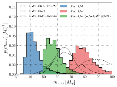
There are features in the black hole mass spectrum beyond a power-law. Figure 3 shows the astrophysical merger rate density as a function of primary BH mass for the Truncated, Power Law + Peak, Multi Peak and Broken Power Law models. Figure 4, meanwhile, shows the posterior predictive distribution for primary masses, including selection effects. Corner plots showing the constraints for the parameters in each model are available in Appendix B; see Figs. 16, 17 and 18. In Appendix C, we show posterior predictive checks for each model (Fig. 19 and Fig. 23), comparing mock observations predicted by the model to the empirical distribution inferred from GWTC-2.
We turn first to the Broken Power Law model (second panel in Fig. 3), which is characterized by two spectral indices, and , with for , and above the break. We find the data prefer a break at ; 90% credible bounds on the location of this break are denoted by the gray vertical band in the second panel of Fig. 3. For masses above the break, the Broken Power Law model prefers a significantly steeper power-law slope, from before to after. Figure 5 shows the joint posterior on and . We infer that at credibility . The break aligns with the cutoff inferred with GWTC-1 data (Abbott et al., 2019a), and we speculate that the steep drop-off in the merger rate that occurs after may be an imprint of PPSN, which are expected to become important for BH masses around (Woosley & Heger, 2015; Heger & Woosley, 2002; Heger et al., 2003).
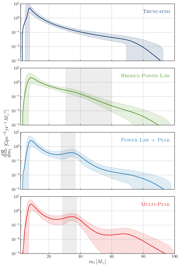
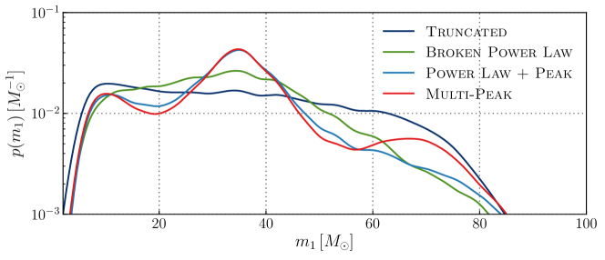
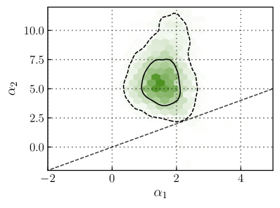
The Power Law + Peak model (third panel of Fig. 3) produces a qualitatively similar fit to the one obtained from the Broken Power Law model. However, a key feature of the Power Law + Peak model is the Gaussian peak at , denoted by the gray vertical band in the third panel of Fig. 3. Evidence for a peak can be seen in Fig. 6, which shows the posterior for , the fraction of systems that belong to the Gaussian component. We see that (pure power law) is disfavored. It was envisioned (Talbot & Thrane, 2018) that the power-law component of the Power Law + Peak model would terminate in the vicinity of this peak to create a high-mass gap. However, in order to accommodate the most massive binaries in GWTC-2, the power-law extends to values of .
While the mass spectrum must extend to these high masses, we find that 99% of primary BH masses lie below ; see Table 3. The astrophysical rate density at (the primary mass of \IfEqCaseGW190521AGW190413AGW190413_052954GW190719AGW190719_215514GW190620AGW190620_030421GW190514AGW190514_065416GW190731AGW190731_140936GW190503AGW190503_185404GW190602AGW190602_175927GW190929AGW190929_012149GW190517AGW190517_055101GW190915AGW190915_235702GW190425AGW190425GW190512AGW190512_180714GW190630AGW190630_185205GW190521AGW190521GW190413BGW190413_134308GW190924AGW190924_021846GW190930AGW190930_133541GW190706AGW190706_222641GW190408AGW190408_181802GW190909AGW190909_114149GW190728AGW190728_064510GW190426AGW190426_152155GW190412AGW190412GW190720AGW190720_000836GW190521BGW190521_074359GW190910AGW190910_112807GW190803AGW190803_022701GW190519AGW190519_153544GW190708AGW190708_232457GW190527AGW190527_092055GW190513AGW190513_205428GW190424AGW190424_180648GW190727AGW190727_060333GW190814AGW190814GW190707AGW190707_093326GW190828AGW190828_063405GW190828BGW190828_065509GW190701AGW190701_203306GW190421AGW190421_213856) is two orders of magnitude lower than the rate density at . However, because of selection effects, the posterior predictive distribution skews to much higher masses, as seen in Fig. 4, so that the probability of detecting at least one event with after observing 44 BBH events drawn from the Power Law + Peak posterior predictive distribution of Fig. 4 is high: .
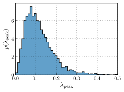
We cannot determine whether the high-mass events of GWTC-2 belong to a distinct subpopulation rather than a high-mass tail of the normal BBH population. An additional subpopulation may be expected if high-mass BHs have a different origin from low mass ones; for example, if they are the products of hierarchical mergers (Fishbach et al., 2017; Gerosa & Berti, 2017; Chatziioannou et al., 2019; Doctor et al., 2019; Kimball et al., 2020a). Using the Multi Peak model (bottom panel in Fig. 3), which allows for a second high-mass Gaussian component at in addition to the Gaussian component at , we find that the addition of a second Gaussian peak is not preferred by the data. The Multi Peak model is mildly disfavored compared to Power Law + Peak, with a (or Bayes factor ) for Multi Peak relative to Power Law + Peak. A similar conclusion is found using the Multi Spin model; as discussed in Section 5.2, we find hints, but no significant evidence for subpopulations with distinct spin distributions.
Within the framework of the Broken Power Law, Power Law + Peak and Multi Peak models, the most massive event, \IfEqCaseGW190521AGW190413AGW190413_052954GW190719AGW190719_215514GW190620AGW190620_030421GW190514AGW190514_065416GW190731AGW190731_140936GW190503AGW190503_185404GW190602AGW190602_175927GW190929AGW190929_012149GW190517AGW190517_055101GW190915AGW190915_235702GW190425AGW190425GW190512AGW190512_180714GW190630AGW190630_185205GW190521AGW190521GW190413BGW190413_134308GW190924AGW190924_021846GW190930AGW190930_133541GW190706AGW190706_222641GW190408AGW190408_181802GW190909AGW190909_114149GW190728AGW190728_064510GW190426AGW190426_152155GW190412AGW190412GW190720AGW190720_000836GW190521BGW190521_074359GW190910AGW190910_112807GW190803AGW190803_022701GW190519AGW190519_153544GW190708AGW190708_232457GW190527AGW190527_092055GW190513AGW190513_205428GW190424AGW190424_180648GW190727AGW190727_060333GW190814AGW190814GW190707AGW190707_093326GW190828AGW190828_063405GW190828BGW190828_065509GW190701AGW190701_203306GW190421AGW190421_213856, appears to be a normal member of the BBH population in the context of the other GWTC-2 events (see Appendix C.2). The event \IfEqCaseGW190521AGW190413AGW190413_052954GW190719AGW190719_215514GW190620AGW190620_030421GW190514AGW190514_065416GW190731AGW190731_140936GW190503AGW190503_185404GW190602AGW190602_175927GW190929AGW190929_012149GW190517AGW190517_055101GW190915AGW190915_235702GW190425AGW190425GW190512AGW190512_180714GW190630AGW190630_185205GW190521AGW190521GW190413BGW190413_134308GW190924AGW190924_021846GW190930AGW190930_133541GW190706AGW190706_222641GW190408AGW190408_181802GW190909AGW190909_114149GW190728AGW190728_064510GW190426AGW190426_152155GW190412AGW190412GW190720AGW190720_000836GW190521BGW190521_074359GW190910AGW190910_112807GW190803AGW190803_022701GW190519AGW190519_153544GW190708AGW190708_232457GW190527AGW190527_092055GW190513AGW190513_205428GW190424AGW190424_180648GW190727AGW190727_060333GW190814AGW190814GW190707AGW190707_093326GW190828AGW190828_063405GW190828BGW190828_065509GW190701AGW190701_203306GW190421AGW190421_213856 is an outlier if we consider it in the context of GWTC-1 with the Truncated model, but we interpret this as a limitation of the Truncated model (see Fig. 2; Abbott et al., 2020f).
The GWTC-1 detections showed that BHs more massive than merge relatively rarely, based on simple extrapolations from below . With GWTC-2, we are beginning to resolve the shape of the primary BH mass spectrum above . The implications are not yet clear, but there are intriguing possibilities. One hypothesis is that the events with are simply the high-mass tail of the ordinary BBH population, and do not form through a distinct channel. For example, if the lower edge of the PPSN gap may be modeled as a smooth tapering rather than a sharp cutoff, the feature at may represent the onset of pair-instability. This explanation may pose challenges to our understanding of stellar evolution since the pair-instability cutoff of BH masses at is thought to be relatively abrupt (Woosley et al., 2002; Woosley, 2017; Farmer et al., 2019), even though its precise location is uncertain (Mapelli et al., 2020; Spera & Mapelli, 2017; Giacobbo et al., 2017; van Son et al., 2020; Farmer et al., 2020; Croon et al., 2020; Marchant & Moriya, 2020). If the PPSN cutoff is indeed sharp and all observed BBH systems lie below the PPSN gap, the cutoff must occur at relatively high masses; in the Truncated model, (or, excluding the most massive event, \IfEqCaseGW190521AGW190413AGW190413_052954GW190719AGW190719_215514GW190620AGW190620_030421GW190514AGW190514_065416GW190731AGW190731_140936GW190503AGW190503_185404GW190602AGW190602_175927GW190929AGW190929_012149GW190517AGW190517_055101GW190915AGW190915_235702GW190425AGW190425GW190512AGW190512_180714GW190630AGW190630_185205GW190521AGW190521GW190413BGW190413_134308GW190924AGW190924_021846GW190930AGW190930_133541GW190706AGW190706_222641GW190408AGW190408_181802GW190909AGW190909_114149GW190728AGW190728_064510GW190426AGW190426_152155GW190412AGW190412GW190720AGW190720_000836GW190521BGW190521_074359GW190910AGW190910_112807GW190803AGW190803_022701GW190519AGW190519_153544GW190708AGW190708_232457GW190527AGW190527_092055GW190513AGW190513_205428GW190424AGW190424_180648GW190727AGW190727_060333GW190814AGW190814GW190707AGW190707_093326GW190828AGW190828_063405GW190828BGW190828_065509GW190701AGW190701_203306GW190421AGW190421_213856, ). This may have significant implications for nuclear (Farmer et al., 2020) and particle (Croon et al., 2020; Ziegler & Freese, 2020) physics.
Another hypothesis is that the events with constitute a distinct population, created, for example, from hierarchical mergers of lower mass binaries in globular clusters or galactic nuclei (Miller & Hamilton, 2002a; Antonini & Rasio, 2016; Kimpson et al., 2016; Rodriguez et al., 2018; Yang et al., 2019; Arca Sedda, 2020a). Alternatively, the high-mass gap might be populated from low-metallicity stellar mergers in young star clusters, the remnants of which can merge dynamically (Carlo et al., 2019a, b), BH growth through accretion (Roupas & Kazanas, 2019; Rice & Zhang, 2020; Natarajan, 2020; Safarzadeh & Haiman, 2020), or Population III stellar remnants with large hydrogen envelopes (Tanikawa et al., 2020; Farrell et al., 2020; Liu & Bromm, 2020).
The BBH primary mass distribution exhibits a global maximum between and . Figure 7 shows the joint posterior for the and parameters inferred using the Power Law + Peak and Broken Power Law mass models, including only BBH events with . Recall that, while the Truncated model has a sharp cutoff at , the remaining models implement a smooth turn-on of width above , causing the mass spectrum to peak and turn over between , and (Talbot & Thrane, 2018). Using both the Broken Power Law model and the Power Law + Peak model, we find that the primary mass spectrum does not decrease monotonically from . Rather, it turns over at (Power Law + Peak model) or (Broken Power Law model). In other words, the mass distribution must turn over at , with credibility (assuming the Power Law + Peak model) or credibility (Broken Power Law model). As seen in Fig. 7, if the BH low-mass cutoff is sharp (), then . Conversely, if the BH mass spectrum extends below , an extended turn-on is required. These results support the existence of a low-mass gap (or dip) between (the secondary mass of \IfEqCaseGW190814AGW190413AGW190413_052954GW190719AGW190719_215514GW190620AGW190620_030421GW190514AGW190514_065416GW190731AGW190731_140936GW190503AGW190503_185404GW190602AGW190602_175927GW190929AGW190929_012149GW190517AGW190517_055101GW190915AGW190915_235702GW190425AGW190425GW190512AGW190512_180714GW190630AGW190630_185205GW190521AGW190521GW190413BGW190413_134308GW190924AGW190924_021846GW190930AGW190930_133541GW190706AGW190706_222641GW190408AGW190408_181802GW190909AGW190909_114149GW190728AGW190728_064510GW190426AGW190426_152155GW190412AGW190412GW190720AGW190720_000836GW190521BGW190521_074359GW190910AGW190910_112807GW190803AGW190803_022701GW190519AGW190519_153544GW190708AGW190708_232457GW190527AGW190527_092055GW190513AGW190513_205428GW190424AGW190424_180648GW190727AGW190727_060333GW190814AGW190814GW190707AGW190707_093326GW190828AGW190828_063405GW190828BGW190828_065509GW190701AGW190701_203306GW190421AGW190421_213856; the most massive component mass observed below ) and , strengthening results from Fishbach et al. (2020a), although we cannot determine whether the low-mass gap is empty.
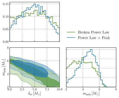
Since our models do not permit additional features beyond a smooth turn on to a power law at low masses, they struggle to accommodate \IfEqCaseGW190814AGW190413AGW190413_052954GW190719AGW190719_215514GW190620AGW190620_030421GW190514AGW190514_065416GW190731AGW190731_140936GW190503AGW190503_185404GW190602AGW190602_175927GW190929AGW190929_012149GW190517AGW190517_055101GW190915AGW190915_235702GW190425AGW190425GW190512AGW190512_180714GW190630AGW190630_185205GW190521AGW190521GW190413BGW190413_134308GW190924AGW190924_021846GW190930AGW190930_133541GW190706AGW190706_222641GW190408AGW190408_181802GW190909AGW190909_114149GW190728AGW190728_064510GW190426AGW190426_152155GW190412AGW190412GW190720AGW190720_000836GW190521BGW190521_074359GW190910AGW190910_112807GW190803AGW190803_022701GW190519AGW190519_153544GW190708AGW190708_232457GW190527AGW190527_092055GW190513AGW190513_205428GW190424AGW190424_180648GW190727AGW190727_060333GW190814AGW190814GW190707AGW190707_093326GW190828AGW190828_063405GW190828BGW190828_065509GW190701AGW190701_203306GW190421AGW190421_213856 (with secondary mass at ). If \IfEqCaseGW190814AGW190413AGW190413_052954GW190719AGW190719_215514GW190620AGW190620_030421GW190514AGW190514_065416GW190731AGW190731_140936GW190503AGW190503_185404GW190602AGW190602_175927GW190929AGW190929_012149GW190517AGW190517_055101GW190915AGW190915_235702GW190425AGW190425GW190512AGW190512_180714GW190630AGW190630_185205GW190521AGW190521GW190413BGW190413_134308GW190924AGW190924_021846GW190930AGW190930_133541GW190706AGW190706_222641GW190408AGW190408_181802GW190909AGW190909_114149GW190728AGW190728_064510GW190426AGW190426_152155GW190412AGW190412GW190720AGW190720_000836GW190521BGW190521_074359GW190910AGW190910_112807GW190803AGW190803_022701GW190519AGW190519_153544GW190708AGW190708_232457GW190527AGW190527_092055GW190513AGW190513_205428GW190424AGW190424_180648GW190727AGW190727_060333GW190814AGW190814GW190707AGW190707_093326GW190828AGW190828_063405GW190828BGW190828_065509GW190701AGW190701_203306GW190421AGW190421_213856 is a BBH system, the minimum BH mass must extend to (see the dashed histograms in Fig. 8a). In Fig. 8b we show how the inclusion/exclusion of \IfEqCaseGW190814AGW190413AGW190413_052954GW190719AGW190719_215514GW190620AGW190620_030421GW190514AGW190514_065416GW190731AGW190731_140936GW190503AGW190503_185404GW190602AGW190602_175927GW190929AGW190929_012149GW190517AGW190517_055101GW190915AGW190915_235702GW190425AGW190425GW190512AGW190512_180714GW190630AGW190630_185205GW190521AGW190521GW190413BGW190413_134308GW190924AGW190924_021846GW190930AGW190930_133541GW190706AGW190706_222641GW190408AGW190408_181802GW190909AGW190909_114149GW190728AGW190728_064510GW190426AGW190426_152155GW190412AGW190412GW190720AGW190720_000836GW190521BGW190521_074359GW190910AGW190910_112807GW190803AGW190803_022701GW190519AGW190519_153544GW190708AGW190708_232457GW190527AGW190527_092055GW190513AGW190513_205428GW190424AGW190424_180648GW190727AGW190727_060333GW190814AGW190814GW190707AGW190707_093326GW190828AGW190828_063405GW190828BGW190828_065509GW190701AGW190701_203306GW190421AGW190421_213856 affects the shape of the primary mass distribution below . This effect can also be seen in the values inferred with/without \IfEqCaseGW190814AGW190413AGW190413_052954GW190719AGW190719_215514GW190620AGW190620_030421GW190514AGW190514_065416GW190731AGW190731_140936GW190503AGW190503_185404GW190602AGW190602_175927GW190929AGW190929_012149GW190517AGW190517_055101GW190915AGW190915_235702GW190425AGW190425GW190512AGW190512_180714GW190630AGW190630_185205GW190521AGW190521GW190413BGW190413_134308GW190924AGW190924_021846GW190930AGW190930_133541GW190706AGW190706_222641GW190408AGW190408_181802GW190909AGW190909_114149GW190728AGW190728_064510GW190426AGW190426_152155GW190412AGW190412GW190720AGW190720_000836GW190521BGW190521_074359GW190910AGW190910_112807GW190803AGW190803_022701GW190519AGW190519_153544GW190708AGW190708_232457GW190527AGW190527_092055GW190513AGW190513_205428GW190424AGW190424_180648GW190727AGW190727_060333GW190814AGW190814GW190707AGW190707_093326GW190828AGW190828_063405GW190828BGW190828_065509GW190701AGW190701_203306GW190421AGW190421_213856, shown in Table 3. Assuming the Truncated and Power Law + Peak models, the posteriors inferred with \IfEqCaseGW190814AGW190413AGW190413_052954GW190719AGW190719_215514GW190620AGW190620_030421GW190514AGW190514_065416GW190731AGW190731_140936GW190503AGW190503_185404GW190602AGW190602_175927GW190929AGW190929_012149GW190517AGW190517_055101GW190915AGW190915_235702GW190425AGW190425GW190512AGW190512_180714GW190630AGW190630_185205GW190521AGW190521GW190413BGW190413_134308GW190924AGW190924_021846GW190930AGW190930_133541GW190706AGW190706_222641GW190408AGW190408_181802GW190909AGW190909_114149GW190728AGW190728_064510GW190426AGW190426_152155GW190412AGW190412GW190720AGW190720_000836GW190521BGW190521_074359GW190910AGW190910_112807GW190803AGW190803_022701GW190519AGW190519_153544GW190708AGW190708_232457GW190527AGW190527_092055GW190513AGW190513_205428GW190424AGW190424_180648GW190727AGW190727_060333GW190814AGW190814GW190707AGW190707_093326GW190828AGW190828_063405GW190828BGW190828_065509GW190701AGW190701_203306GW190421AGW190421_213856 lie at the and percentiles, respectively, of the posteriors obtained without \IfEqCaseGW190814AGW190413AGW190413_052954GW190719AGW190719_215514GW190620AGW190620_030421GW190514AGW190514_065416GW190731AGW190731_140936GW190503AGW190503_185404GW190602AGW190602_175927GW190929AGW190929_012149GW190517AGW190517_055101GW190915AGW190915_235702GW190425AGW190425GW190512AGW190512_180714GW190630AGW190630_185205GW190521AGW190521GW190413BGW190413_134308GW190924AGW190924_021846GW190930AGW190930_133541GW190706AGW190706_222641GW190408AGW190408_181802GW190909AGW190909_114149GW190728AGW190728_064510GW190426AGW190426_152155GW190412AGW190412GW190720AGW190720_000836GW190521BGW190521_074359GW190910AGW190910_112807GW190803AGW190803_022701GW190519AGW190519_153544GW190708AGW190708_232457GW190527AGW190527_092055GW190513AGW190513_205428GW190424AGW190424_180648GW190727AGW190727_060333GW190814AGW190814GW190707AGW190707_093326GW190828AGW190828_063405GW190828BGW190828_065509GW190701AGW190701_203306GW190421AGW190421_213856. Even using the Broken Power Law model, which admits greater overlap in the 1-dimensional posteriors inferred with/without \IfEqCaseGW190814AGW190413AGW190413_052954GW190719AGW190719_215514GW190620AGW190620_030421GW190514AGW190514_065416GW190731AGW190731_140936GW190503AGW190503_185404GW190602AGW190602_175927GW190929AGW190929_012149GW190517AGW190517_055101GW190915AGW190915_235702GW190425AGW190425GW190512AGW190512_180714GW190630AGW190630_185205GW190521AGW190521GW190413BGW190413_134308GW190924AGW190924_021846GW190930AGW190930_133541GW190706AGW190706_222641GW190408AGW190408_181802GW190909AGW190909_114149GW190728AGW190728_064510GW190426AGW190426_152155GW190412AGW190412GW190720AGW190720_000836GW190521BGW190521_074359GW190910AGW190910_112807GW190803AGW190803_022701GW190519AGW190519_153544GW190708AGW190708_232457GW190527AGW190527_092055GW190513AGW190513_205428GW190424AGW190424_180648GW190727AGW190727_060333GW190814AGW190814GW190707AGW190707_093326GW190828AGW190828_063405GW190828BGW190828_065509GW190701AGW190701_203306GW190421AGW190421_213856, the addition of \IfEqCaseGW190814AGW190413AGW190413_052954GW190719AGW190719_215514GW190620AGW190620_030421GW190514AGW190514_065416GW190731AGW190731_140936GW190503AGW190503_185404GW190602AGW190602_175927GW190929AGW190929_012149GW190517AGW190517_055101GW190915AGW190915_235702GW190425AGW190425GW190512AGW190512_180714GW190630AGW190630_185205GW190521AGW190521GW190413BGW190413_134308GW190924AGW190924_021846GW190930AGW190930_133541GW190706AGW190706_222641GW190408AGW190408_181802GW190909AGW190909_114149GW190728AGW190728_064510GW190426AGW190426_152155GW190412AGW190412GW190720AGW190720_000836GW190521BGW190521_074359GW190910AGW190910_112807GW190803AGW190803_022701GW190519AGW190519_153544GW190708AGW190708_232457GW190527AGW190527_092055GW190513AGW190513_205428GW190424AGW190424_180648GW190727AGW190727_060333GW190814AGW190814GW190707AGW190707_093326GW190828AGW190828_063405GW190828BGW190828_065509GW190701AGW190701_203306GW190421AGW190421_213856 significantly shifts the two-dimensional posterior and the inferred mass spectrum. Assuming the Broken Power Law model with \IfEqCaseGW190814AGW190413AGW190413_052954GW190719AGW190719_215514GW190620AGW190620_030421GW190514AGW190514_065416GW190731AGW190731_140936GW190503AGW190503_185404GW190602AGW190602_175927GW190929AGW190929_012149GW190517AGW190517_055101GW190915AGW190915_235702GW190425AGW190425GW190512AGW190512_180714GW190630AGW190630_185205GW190521AGW190521GW190413BGW190413_134308GW190924AGW190924_021846GW190930AGW190930_133541GW190706AGW190706_222641GW190408AGW190408_181802GW190909AGW190909_114149GW190728AGW190728_064510GW190426AGW190426_152155GW190412AGW190412GW190720AGW190720_000836GW190521BGW190521_074359GW190910AGW190910_112807GW190803AGW190803_022701GW190519AGW190519_153544GW190708AGW190708_232457GW190527AGW190527_092055GW190513AGW190513_205428GW190424AGW190424_180648GW190727AGW190727_060333GW190814AGW190814GW190707AGW190707_093326GW190828AGW190828_063405GW190828BGW190828_065509GW190701AGW190701_203306GW190421AGW190421_213856, the mass at which the mass spectrum turns over is shifted down to , which is inconsistent with the turnover mass (the low-mass local maximum) inferred without \IfEqCaseGW190814AGW190413AGW190413_052954GW190719AGW190719_215514GW190620AGW190620_030421GW190514AGW190514_065416GW190731AGW190731_140936GW190503AGW190503_185404GW190602AGW190602_175927GW190929AGW190929_012149GW190517AGW190517_055101GW190915AGW190915_235702GW190425AGW190425GW190512AGW190512_180714GW190630AGW190630_185205GW190521AGW190521GW190413BGW190413_134308GW190924AGW190924_021846GW190930AGW190930_133541GW190706AGW190706_222641GW190408AGW190408_181802GW190909AGW190909_114149GW190728AGW190728_064510GW190426AGW190426_152155GW190412AGW190412GW190720AGW190720_000836GW190521BGW190521_074359GW190910AGW190910_112807GW190803AGW190803_022701GW190519AGW190519_153544GW190708AGW190708_232457GW190527AGW190527_092055GW190513AGW190513_205428GW190424AGW190424_180648GW190727AGW190727_060333GW190814AGW190814GW190707AGW190707_093326GW190828AGW190828_063405GW190828BGW190828_065509GW190701AGW190701_203306GW190421AGW190421_213856, . This indicates a failure of our models to fit \IfEqCaseGW190814AGW190413AGW190413_052954GW190719AGW190719_215514GW190620AGW190620_030421GW190514AGW190514_065416GW190731AGW190731_140936GW190503AGW190503_185404GW190602AGW190602_175927GW190929AGW190929_012149GW190517AGW190517_055101GW190915AGW190915_235702GW190425AGW190425GW190512AGW190512_180714GW190630AGW190630_185205GW190521AGW190521GW190413BGW190413_134308GW190924AGW190924_021846GW190930AGW190930_133541GW190706AGW190706_222641GW190408AGW190408_181802GW190909AGW190909_114149GW190728AGW190728_064510GW190426AGW190426_152155GW190412AGW190412GW190720AGW190720_000836GW190521BGW190521_074359GW190910AGW190910_112807GW190803AGW190803_022701GW190519AGW190519_153544GW190708AGW190708_232457GW190527AGW190527_092055GW190513AGW190513_205428GW190424AGW190424_180648GW190727AGW190727_060333GW190814AGW190814GW190707AGW190707_093326GW190828AGW190828_063405GW190828BGW190828_065509GW190701AGW190701_203306GW190421AGW190421_213856 together with the BBH systems of GWTC-2. This finding is supported by additional studies described in Appendix C.3. Because \IfEqCaseGW190814AGW190413AGW190413_052954GW190719AGW190719_215514GW190620AGW190620_030421GW190514AGW190514_065416GW190731AGW190731_140936GW190503AGW190503_185404GW190602AGW190602_175927GW190929AGW190929_012149GW190517AGW190517_055101GW190915AGW190915_235702GW190425AGW190425GW190512AGW190512_180714GW190630AGW190630_185205GW190521AGW190521GW190413BGW190413_134308GW190924AGW190924_021846GW190930AGW190930_133541GW190706AGW190706_222641GW190408AGW190408_181802GW190909AGW190909_114149GW190728AGW190728_064510GW190426AGW190426_152155GW190412AGW190412GW190720AGW190720_000836GW190521BGW190521_074359GW190910AGW190910_112807GW190803AGW190803_022701GW190519AGW190519_153544GW190708AGW190708_232457GW190527AGW190527_092055GW190513AGW190513_205428GW190424AGW190424_180648GW190727AGW190727_060333GW190814AGW190814GW190707AGW190707_093326GW190828AGW190828_063405GW190828BGW190828_065509GW190701AGW190701_203306GW190421AGW190421_213856 is a population outlier with respect to the BBH events of GWTC-2 , we exclude it from the analyses here unless otherwise indicated.
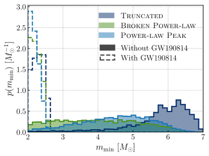
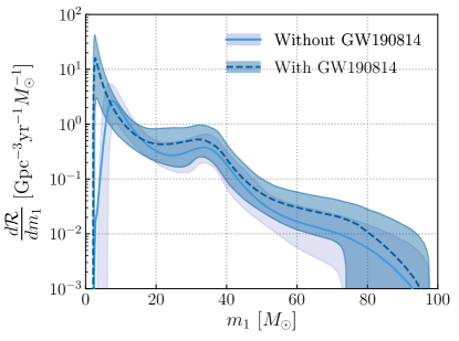
The distribution of mass ratios is broad. The GWTC-1 events are all individually consistent with . Describing the conditional mass-ratio distribution as a power law , a population analysis of GWTC-1 allowed (our maximum prior bound), consistent with a mass-ratio distribution sharply peaked at equal-mass pairings (Abbott et al., 2019a; Roulet & Zaldarriaga, 2019; Fishbach & Holz, 2020b). GWTC-2 saw the first detections of confidently asymmetric systems: \IfEqCaseGW190412AGW190413AGW190413_052954GW190719AGW190719_215514GW190620AGW190620_030421GW190514AGW190514_065416GW190731AGW190731_140936GW190503AGW190503_185404GW190602AGW190602_175927GW190929AGW190929_012149GW190517AGW190517_055101GW190915AGW190915_235702GW190425AGW190425GW190512AGW190512_180714GW190630AGW190630_185205GW190521AGW190521GW190413BGW190413_134308GW190924AGW190924_021846GW190930AGW190930_133541GW190706AGW190706_222641GW190408AGW190408_181802GW190909AGW190909_114149GW190728AGW190728_064510GW190426AGW190426_152155GW190412AGW190412GW190720AGW190720_000836GW190521BGW190521_074359GW190910AGW190910_112807GW190803AGW190803_022701GW190519AGW190519_153544GW190708AGW190708_232457GW190527AGW190527_092055GW190513AGW190513_205428GW190424AGW190424_180648GW190727AGW190727_060333GW190814AGW190814GW190707AGW190707_093326GW190828AGW190828_063405GW190828BGW190828_065509GW190701AGW190701_203306GW190421AGW190421_213856 (Abbott et al., 2020a) and GW190814 (Abbott et al., 2020b). Excluding \IfEqCaseGW190814AGW190413AGW190413_052954GW190719AGW190719_215514GW190620AGW190620_030421GW190514AGW190514_065416GW190731AGW190731_140936GW190503AGW190503_185404GW190602AGW190602_175927GW190929AGW190929_012149GW190517AGW190517_055101GW190915AGW190915_235702GW190425AGW190425GW190512AGW190512_180714GW190630AGW190630_185205GW190521AGW190521GW190413BGW190413_134308GW190924AGW190924_021846GW190930AGW190930_133541GW190706AGW190706_222641GW190408AGW190408_181802GW190909AGW190909_114149GW190728AGW190728_064510GW190426AGW190426_152155GW190412AGW190412GW190720AGW190720_000836GW190521BGW190521_074359GW190910AGW190910_112807GW190803AGW190803_022701GW190519AGW190519_153544GW190708AGW190708_232457GW190527AGW190527_092055GW190513AGW190513_205428GW190424AGW190424_180648GW190727AGW190727_060333GW190814AGW190814GW190707AGW190707_093326GW190828AGW190828_063405GW190828BGW190828_065509GW190701AGW190701_203306GW190421AGW190421_213856, our reconstruction of the mass ratio distribution is consistent with the results published in Abbott et al. (2020a): for the Power Law + Peak model and for the Broken Power Law model. We rule out distributions that are sharply peaked around , with (Power Law + Peak) and (Broken Power Law) at 90% credibility. However, we also disfavor distributions that prefer unequal-mass pairings, with at % (Power Law + Peak) and % (Broken Power Law) credibility. We find that 90% of systems in the underlying population have mass ratios .
5.2 Spin Distribution
In this subsection, we highlight the results from the Gaussian, Default, and Multi Spin models. We fix the redshift distribution to a Non-Evolving merger rate. The Gaussian and Multi Spin models assume the mass distributions described in Appendix D.2 and D.3, respectively. For the Default spin model, we employ the Power Law + Peak mass model, simultaneously fitting the mass and spin distribution as in the previous subsection.
We observe spin-induced general relativistic precession of the orbital plane. As two BHs merge, the morphology of the resulting gravitational waveform depends on their spins. The spin-dependence of a gravitational waveform is determined in part by two phenomenological parameters. First, the effective inspiral spin parameter quantifies the spin components aligned with the orbital angular momentum (Damour, 2001):
| (5) |
Here, and are the dimensionless component spins, defined by where is the spin angular momentum of component , and and are the misalignment angles between the component spins and the orbital angular momentum. Second, spins with components perpendicular to the orbital angular momentum drive relativistic precession of the orbital plane (Apostolatos et al., 1994). The effect is quantified by the effective precession spin parameter (Schmidt et al., 2012; Hannam et al., 2014; Schmidt et al., 2015)
| (6) |
A non-zero value of indicates the presence of relativistic spin-induced precession of the orbital plane. Although the component spin tilts and appearing in Eqs. (5) and (6) generically evolve over the course of a binary inspiral, and are themselves approximately conserved quantities (Kidder, 1995; Schmidt et al., 2015).
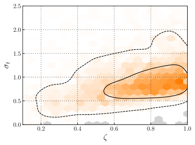
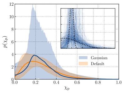
The first unambiguous measurements of BH spin in gravitational-wave astronomy came from analyses of the BBH event GW151226. This system had at 99% credibility, with at least one of its components having spin magnitude , and spin misalignment angles consistent with (Abbott et al., 2016b). While analyses of GWTC-1 found no clear evidence for spin in the other events in GWTC-1 (Miller et al. 2020, but also see Zackay et al. 2019 and Huang et al. 2020), GWTC-1 is collectively inconsistent with a population of non-spinning BHs, if one allows for both spinning and non-spinning subpopulations (Kimball et al., 2020a). Moreover, population analyses of GWTC-1 mildly disfavor the scenario in which all spins are perfectly aligned (), although the degree of misalignment is degenerate with the spin magnitude distribution (Farr et al., 2017, 2018; Tiwari et al., 2018; Abbott et al., 2019a; Wysocki et al., 2019b).
In GWTC-2, additional BBH events are observed with confidently positive effective inspiral spin parameter. No individual event is observed with confidently negative (Abbott et al., 2020c). Several events, including \IfEqCaseGW190521AGW190413AGW190413_052954GW190719AGW190719_215514GW190620AGW190620_030421GW190514AGW190514_065416GW190731AGW190731_140936GW190503AGW190503_185404GW190602AGW190602_175927GW190929AGW190929_012149GW190517AGW190517_055101GW190915AGW190915_235702GW190425AGW190425GW190512AGW190512_180714GW190630AGW190630_185205GW190521AGW190521GW190413BGW190413_134308GW190924AGW190924_021846GW190930AGW190930_133541GW190706AGW190706_222641GW190408AGW190408_181802GW190909AGW190909_114149GW190728AGW190728_064510GW190426AGW190426_152155GW190412AGW190412GW190720AGW190720_000836GW190521BGW190521_074359GW190910AGW190910_112807GW190803AGW190803_022701GW190519AGW190519_153544GW190708AGW190708_232457GW190527AGW190527_092055GW190513AGW190513_205428GW190424AGW190424_180648GW190727AGW190727_060333GW190814AGW190814GW190707AGW190707_093326GW190828AGW190828_063405GW190828BGW190828_065509GW190701AGW190701_203306GW190421AGW190421_213856 (Abbott et al., 2020e, f) and \IfEqCaseGW190412AGW190413AGW190413_052954GW190719AGW190719_215514GW190620AGW190620_030421GW190514AGW190514_065416GW190731AGW190731_140936GW190503AGW190503_185404GW190602AGW190602_175927GW190929AGW190929_012149GW190517AGW190517_055101GW190915AGW190915_235702GW190425AGW190425GW190512AGW190512_180714GW190630AGW190630_185205GW190521AGW190521GW190413BGW190413_134308GW190924AGW190924_021846GW190930AGW190930_133541GW190706AGW190706_222641GW190408AGW190408_181802GW190909AGW190909_114149GW190728AGW190728_064510GW190426AGW190426_152155GW190412AGW190412GW190720AGW190720_000836GW190521BGW190521_074359GW190910AGW190910_112807GW190803AGW190803_022701GW190519AGW190519_153544GW190708AGW190708_232457GW190527AGW190527_092055GW190513AGW190513_205428GW190424AGW190424_180648GW190727AGW190727_060333GW190814AGW190814GW190707AGW190707_093326GW190828AGW190828_063405GW190828BGW190828_065509GW190701AGW190701_203306GW190421AGW190421_213856 (Abbott et al., 2020a), show moderate evidence for non-zero , but no single event unambiguously exhibits spin-induced precession (Abbott et al., 2020c).
the right side of Fig. 9, the dark blue curve and shaded blue region mark the median and 90% credible bound, respectively, on as inferred by the Gaussian model. While the blue region in this figure suggests a distribution that peaks at , there are in fact two morphologies preferred by the data according to the Gaussian model: the recovered distribution is either broad—or narrowly peaked at . This is illustrated by the inset, in which we plot an ensemble of distributions corresponding to individual draws from the posterior; the dashed black curves highlight traces representative of the two permitted morphologies.
As mentioned above, \IfEqCaseGW190521AGW190413AGW190413_052954GW190719AGW190719_215514GW190620AGW190620_030421GW190514AGW190514_065416GW190731AGW190731_140936GW190503AGW190503_185404GW190602AGW190602_175927GW190929AGW190929_012149GW190517AGW190517_055101GW190915AGW190915_235702GW190425AGW190425GW190512AGW190512_180714GW190630AGW190630_185205GW190521AGW190521GW190413BGW190413_134308GW190924AGW190924_021846GW190930AGW190930_133541GW190706AGW190706_222641GW190408AGW190408_181802GW190909AGW190909_114149GW190728AGW190728_064510GW190426AGW190426_152155GW190412AGW190412GW190720AGW190720_000836GW190521BGW190521_074359GW190910AGW190910_112807GW190803AGW190803_022701GW190519AGW190519_153544GW190708AGW190708_232457GW190527AGW190527_092055GW190513AGW190513_205428GW190424AGW190424_180648GW190727AGW190727_060333GW190814AGW190814GW190707AGW190707_093326GW190828AGW190828_063405GW190828BGW190828_065509GW190701AGW190701_203306GW190421AGW190421_213856 and \IfEqCaseGW190412AGW190413AGW190413_052954GW190719AGW190719_215514GW190620AGW190620_030421GW190514AGW190514_065416GW190731AGW190731_140936GW190503AGW190503_185404GW190602AGW190602_175927GW190929AGW190929_012149GW190517AGW190517_055101GW190915AGW190915_235702GW190425AGW190425GW190512AGW190512_180714GW190630AGW190630_185205GW190521AGW190521GW190413BGW190413_134308GW190924AGW190924_021846GW190930AGW190930_133541GW190706AGW190706_222641GW190408AGW190408_181802GW190909AGW190909_114149GW190728AGW190728_064510GW190426AGW190426_152155GW190412AGW190412GW190720AGW190720_000836GW190521BGW190521_074359GW190910AGW190910_112807GW190803AGW190803_022701GW190519AGW190519_153544GW190708AGW190708_232457GW190527AGW190527_092055GW190513AGW190513_205428GW190424AGW190424_180648GW190727AGW190727_060333GW190814AGW190814GW190707AGW190707_093326GW190828AGW190828_063405GW190828BGW190828_065509GW190701AGW190701_203306GW190421AGW190421_213856 individually show mild evidence of precession, with posteriors shifted away from their respective priors (Abbott et al., 2020a, e, f). To verify that our population-level conclusions are not driven primarily by these two events, we have repeated the Gaussian analysis excluding \IfEqCaseGW190521AGW190413AGW190413_052954GW190719AGW190719_215514GW190620AGW190620_030421GW190514AGW190514_065416GW190731AGW190731_140936GW190503AGW190503_185404GW190602AGW190602_175927GW190929AGW190929_012149GW190517AGW190517_055101GW190915AGW190915_235702GW190425AGW190425GW190512AGW190512_180714GW190630AGW190630_185205GW190521AGW190521GW190413BGW190413_134308GW190924AGW190924_021846GW190930AGW190930_133541GW190706AGW190706_222641GW190408AGW190408_181802GW190909AGW190909_114149GW190728AGW190728_064510GW190426AGW190426_152155GW190412AGW190412GW190720AGW190720_000836GW190521BGW190521_074359GW190910AGW190910_112807GW190803AGW190803_022701GW190519AGW190519_153544GW190708AGW190708_232457GW190527AGW190527_092055GW190513AGW190513_205428GW190424AGW190424_180648GW190727AGW190727_060333GW190814AGW190814GW190707AGW190707_093326GW190828AGW190828_063405GW190828BGW190828_065509GW190701AGW190701_203306GW190421AGW190421_213856 and \IfEqCaseGW190412AGW190413AGW190413_052954GW190719AGW190719_215514GW190620AGW190620_030421GW190514AGW190514_065416GW190731AGW190731_140936GW190503AGW190503_185404GW190602AGW190602_175927GW190929AGW190929_012149GW190517AGW190517_055101GW190915AGW190915_235702GW190425AGW190425GW190512AGW190512_180714GW190630AGW190630_185205GW190521AGW190521GW190413BGW190413_134308GW190924AGW190924_021846GW190930AGW190930_133541GW190706AGW190706_222641GW190408AGW190408_181802GW190909AGW190909_114149GW190728AGW190728_064510GW190426AGW190426_152155GW190412AGW190412GW190720AGW190720_000836GW190521BGW190521_074359GW190910AGW190910_112807GW190803AGW190803_022701GW190519AGW190519_153544GW190708AGW190708_232457GW190527AGW190527_092055GW190513AGW190513_205428GW190424AGW190424_180648GW190727AGW190727_060333GW190814AGW190814GW190707AGW190707_093326GW190828AGW190828_063405GW190828BGW190828_065509GW190701AGW190701_203306GW190421AGW190421_213856. Our results again exclude at a similar level of confidence ( credibility). This implies that the signature of precession observed here is due to the combined influence of many systems with only weakly measured , consistent with expectations from simulation studies (Fairhurst et al., 2019; Wysocki et al., 2019b).
The injection sets used to quantify search selection effects (see Appendix A) contain only events whose component spins are perfectly aligned with their orbital angular momenta. The results in Fig. 9 therefore do not account for systematics possibly affecting our ability to detect events with . The matched filter template banks adopted by the GstLAL and PyCBC search pipelines, for instance, are composed of purely aligned-spin waveforms, and so may have reduced sensitivity to events with high (Harry et al., 2016; Calderón Bustillo et al., 2017). Selection effects can, however, only decrease the efficiency with which events with large in-plane spins are detected; incorporating such effects would further shift the posterior in Fig. 9 Thus, the presence of in-plane spin components is robust to selection effects. The specific preference for , though, may not be. In the future, accurately characterizing the effects of in-plane spins on detection efficiency will be crucial in order to robustly determine the shape of the and distributions.
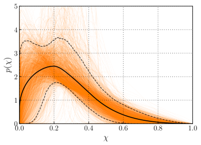
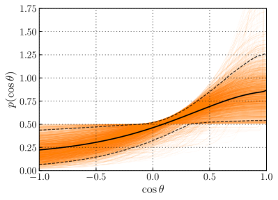
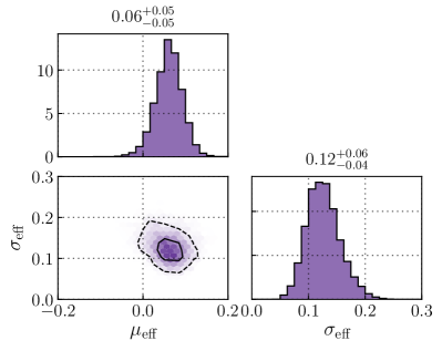
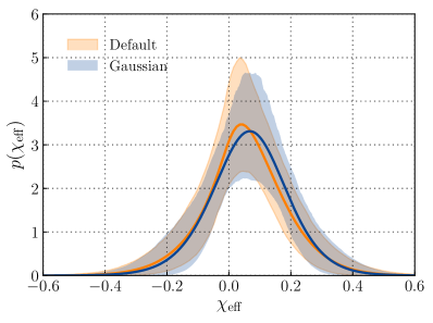
We observe anti-aligned spin, which may suggest the presence of more than one binary formation channel. Using the Gaussian model described in Sec. 3, we infer the presence of systems with negative effective inspiral spin parameter: . Thus, there exist BBH systems with at least one component spin tilted by relative to the orbital angular momenta. Figure 11 shows posteriors for the mean and standard deviation of the distribution, marginalized over , , and the covariance between the effective inspiral spin parameter and the effective precession spin parameter. With a peak at , we find that most systems have small but positive , in agreement with the inference from GWTC-1 (Miller et al., 2020; Roulet & Zaldarriaga, 2019). With GWTC-2, we can now also constrain the width of the distribution. The result, , requires that a nonzero fraction of BBH systems have . Unlike the constraints on the distribution presented above, the results for the presence of negative effective inspiral spin parameter do incorporate selection effects via the prescription described in Sec. 4.
Analysis with the Default spin model is also suggestive of an anisotropic distribution of spin orientations. In Fig. 10, we plot the population distribution of reconstructed using the Default model. While the distribution shows a preference for primarily aligned spins, with , it also exhibits non-vanishing posterior support for , indicating the presence of component spins misaligned by more than . The distribution inferred with the Default model closely matches the distribution inferred using the Gaussian model; compare the orange and blue bands in the right panel of Fig. 11. The two models therefore agree on the fraction of systems with anti-aligned component spins.
To further verify that the apparent presence of events with negative is physical and not an artifact of our choice of models, we repeat our inference of the Gaussian distribution, this time permitting the minimum allowed effective inspiral spin parameter (until now fixed to ) to vary as an additional hyper-parameter to be inferred from the data. When fitting for alongside and , we find that is less than zero at credibility (see Fig. 27 in the Appendix), confirming that the evidence for anti-aligned spin is not an artifact of our parameterization. Allowing to vary yields similar results for the implied distribution, and in particular, the fraction of systems with negative .
The presence of BBH systems with negative effective inspiral spin parameter carries implications for the formation channels that give rise to stellar-mass BBH mergers. BBHs born in the field from isolated stellar progenitors are predicted to contain components whose spins are nearly aligned with their orbital angular momenta, although sufficiently strong supernova kicks might produce modest misalignment (O’Shaughnessy et al., 2017; Stevenson et al., 2017; Gerosa et al., 2018; Rodriguez et al., 2016; Bavera et al., 2019). In contrast, binaries assembled dynamically in dense stellar environments are expected to have randomly oriented component spins, yielding positive or negative with equal probabilities (Kalogera, 2000; Mandel & O’Shaughnessy, 2010; Rodriguez et al., 2016; Zevin et al., 2017; Rodriguez et al., 2018; Doctor et al., 2019).
Using the posteriors for and from Fig. 11, in Fig. 12 we show posteriors for the implied fractions of BBH systems with negative () and positive effective inspiral spin parameter (). Motivated by recent work suggesting that BHs are born with natal spins as small as (Qin et al., 2018; Fuller et al., 2019; Fuller & Ma, 2019; Bavera et al., 2019), as well as the tendency of vanishingly small spins to confound efforts to distinguish between positive and negative (Farr et al., 2018; Abbott et al., 2019a), we include a third bin containing vanishingly small spins between . At 90% credibility, we find that fractions , , and of BBH systems have positive, negative, and vanishing , respectively. All three posterior distributions are peaked away from zero. In particular, at 99% credibility. This result is in contrast to results obtained using GWTC-1 alone, which did not exhibit a confidently non-zero fraction of events with negative (Abbott et al., 2019a; Miller et al., 2020). Additionally, the relatively small fraction of binaries with vanishing spins may provide clues about how BHs gain angular momentum, given recent studies suggesting that most BHs are born slowly rotating (Fuller & Ma, 2019). While we define the vanishing bin to be , the exact choice of width for the vanishing bin does not strongly affect the values of and , relative to one another.
As mentioned above, dynamical formation in dense clusters is not the only astrophysical explanation of negative effective inspiral spin parameter. If stellar progenitors experience both strong natal kicks in supernovae and inefficient spin realignment, of BBH systems formed through isolated binary evolution may have (Rodriguez et al., 2016; O’Shaughnessy et al., 2017; Stevenson et al., 2017; Wysocki et al., 2018), although these results depend on the poorly understood physics of natal kicks and binary interaction via torques and mass transfer. Moreover, we have so far neglected the possibility of other formation channels that may operate in both the field and dynamical regimes. Isolated hierarchical triples, for example, may produce binary mergers with preferentially in-plane component spins (Rodriguez & Antonini, 2018; Antonini et al., 2018; Liu et al., 2019; Fragione & Kocsis, 2020). Mergers in the disks of active galactic nuclei, meanwhile, yield component spins that are preferentially parallel or anti-parallel to a binary’s orbital angular momentum (McKernan et al., 2018; Yang et al., 2019; McKernan et al., 2020).
With these qualifications in mind, if we interpret negative as indicative of dynamical formation in stellar clusters, then our constraints on can be used to infer the fraction of dynamically assembled binaries. We assume that dynamical assembly in dense stellar environments yields a distribution that is symmetric about zero, while isolated binary evolution produces only positive . Among the binaries with non-negligible spin (excluding those in the “vanishing” category above), the fractions and of binaries arising from dynamical and isolated channels are
| (7) | ||||
| (8) |
We find at 90% credibility, suggesting that both the field and the dynamical cluster scenarios contribute to the BBH mergers observed in GWTC-2. Because the relative values of and are not sensitive to the width of the vanishing bin, this conclusion does not depend strongly on the definition of vanishing spin.
At present, we are unable to include a systematic investigation of waveform error in our analysis of anti-aligned spin and orbital precession. However, preliminary studies suggest that waveform error is unlikely to significantly affect this and other results in this paper. For future work, it would be worthwhile to estimate the systematic error using different waveform approximants.
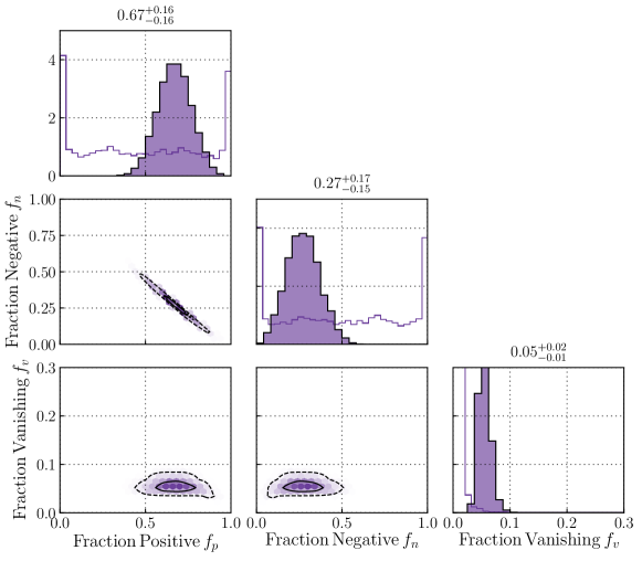
No strong evidence for variation of the spin distribution with mass. BHs born in hierarchical mergers inherit the orbital angular momenta of their progenitor systems, leading to significant spin magnitudes for nearly equal-mass systems (Pretorius, 2005; Berti & Volonteri, 2008; Fishbach et al., 2017; Gerosa et al., 2018; Doctor et al., 2019; Rodriguez et al., 2018, 2019; Kimball et al., 2020a). If hierarchical mergers are present in GWTC-2, then one may expect correlations between the spins and masses of BBH systems, with more massive hierarchical mergers also possessing larger spins. We use the Multi Spin model to explore possible trends in the BBH spin distribution with mass, allowing for a distinct low-mass and high-mass subpopulation (with primary mass distributions parameterized by a power-law and Gaussian, respectively; see Sec. D.3), each with a distinct spin distribution. The low-mass power-law has a weak preference for smaller spins, as compared to the high-mass Gaussian. Both subpopulations disfavor perfectly aligned systems, though the low-mass subpopulation has more support for small misalignments. In spite of these differences, the uncertainties on both of these subpopulations are broad enough that the two are fully consistent with each other, and we cannot confidently claim to detect a mass-dependence to the spin distribution at this stage. This is demonstrated in Fig. 13, which shows the posteriors for the spin distribution hyper-parameters associated with each mass subpopulation. These findings support the results of previous studies on GWTC-1, which could neither exclude nor confidently detect variation of the spin distribution with mass (Safarzadeh et al., 2020; Tiwari, 2020).

5.3 Merger rate and redshift evolution
In this subsection we use the Power Law + Peak and Broken Power Law mass models with the Default spin model, and infer the merger rate using the Non-Evolving redshift model and the Power-law evolution redshift model.
We better constrain the binary black hole merger rate. Assuming a log-uniform prior, we find a BBH merger rate of using the Power Law + Peak mass distribution and the assumption of a non-evolving merger rate density. We find that estimates of the BBH merger rate are robust to our choice of mass model, with excellent agreement between the Power Law + Peak, Broken Power Law, and Multi Peak models. The Truncated model yields a higher merger rate than the other models, but the results agree within statistical uncertainties: .
| Mass model | ||||
|---|---|---|---|---|
| Broken Power Law | ||||
| Power Law + Peak | ||||
| Multi Peak | ||||
Our estimate of the BBH merger rate include only systems with , which notably excludes \IfEqCaseGW190814AGW190413AGW190413_052954GW190719AGW190719_215514GW190620AGW190620_030421GW190514AGW190514_065416GW190731AGW190731_140936GW190503AGW190503_185404GW190602AGW190602_175927GW190929AGW190929_012149GW190517AGW190517_055101GW190915AGW190915_235702GW190425AGW190425GW190512AGW190512_180714GW190630AGW190630_185205GW190521AGW190521GW190413BGW190413_134308GW190924AGW190924_021846GW190930AGW190930_133541GW190706AGW190706_222641GW190408AGW190408_181802GW190909AGW190909_114149GW190728AGW190728_064510GW190426AGW190426_152155GW190412AGW190412GW190720AGW190720_000836GW190521BGW190521_074359GW190910AGW190910_112807GW190803AGW190803_022701GW190519AGW190519_153544GW190708AGW190708_232457GW190527AGW190527_092055GW190513AGW190513_205428GW190424AGW190424_180648GW190727AGW190727_060333GW190814AGW190814GW190707AGW190707_093326GW190828AGW190828_063405GW190828BGW190828_065509GW190701AGW190701_203306GW190421AGW190421_213856. If we calculate the merger rate for all systems down to using our models, thereby including \IfEqCaseGW190814AGW190413AGW190413_052954GW190719AGW190719_215514GW190620AGW190620_030421GW190514AGW190514_065416GW190731AGW190731_140936GW190503AGW190503_185404GW190602AGW190602_175927GW190929AGW190929_012149GW190517AGW190517_055101GW190915AGW190915_235702GW190425AGW190425GW190512AGW190512_180714GW190630AGW190630_185205GW190521AGW190521GW190413BGW190413_134308GW190924AGW190924_021846GW190930AGW190930_133541GW190706AGW190706_222641GW190408AGW190408_181802GW190909AGW190909_114149GW190728AGW190728_064510GW190426AGW190426_152155GW190412AGW190412GW190720AGW190720_000836GW190521BGW190521_074359GW190910AGW190910_112807GW190803AGW190803_022701GW190519AGW190519_153544GW190708AGW190708_232457GW190527AGW190527_092055GW190513AGW190513_205428GW190424AGW190424_180648GW190727AGW190727_060333GW190814AGW190814GW190707AGW190707_093326GW190828AGW190828_063405GW190828BGW190828_065509GW190701AGW190701_203306GW190421AGW190421_213856, we infer a higher merger rate: for the Power Law + Peak model. The reason for this change is that including \IfEqCaseGW190814AGW190413AGW190413_052954GW190719AGW190719_215514GW190620AGW190620_030421GW190514AGW190514_065416GW190731AGW190731_140936GW190503AGW190503_185404GW190602AGW190602_175927GW190929AGW190929_012149GW190517AGW190517_055101GW190915AGW190915_235702GW190425AGW190425GW190512AGW190512_180714GW190630AGW190630_185205GW190521AGW190521GW190413BGW190413_134308GW190924AGW190924_021846GW190930AGW190930_133541GW190706AGW190706_222641GW190408AGW190408_181802GW190909AGW190909_114149GW190728AGW190728_064510GW190426AGW190426_152155GW190412AGW190412GW190720AGW190720_000836GW190521BGW190521_074359GW190910AGW190910_112807GW190803AGW190803_022701GW190519AGW190519_153544GW190708AGW190708_232457GW190527AGW190527_092055GW190513AGW190513_205428GW190424AGW190424_180648GW190727AGW190727_060333GW190814AGW190814GW190707AGW190707_093326GW190828AGW190828_063405GW190828BGW190828_065509GW190701AGW190701_203306GW190421AGW190421_213856 increases the low-mass rate (see Fig. 8b). However, because our mass distribution models do not extrapolate well to (see Section 5.1), the fit with \IfEqCaseGW190814AGW190413AGW190413_052954GW190719AGW190719_215514GW190620AGW190620_030421GW190514AGW190514_065416GW190731AGW190731_140936GW190503AGW190503_185404GW190602AGW190602_175927GW190929AGW190929_012149GW190517AGW190517_055101GW190915AGW190915_235702GW190425AGW190425GW190512AGW190512_180714GW190630AGW190630_185205GW190521AGW190521GW190413BGW190413_134308GW190924AGW190924_021846GW190930AGW190930_133541GW190706AGW190706_222641GW190408AGW190408_181802GW190909AGW190909_114149GW190728AGW190728_064510GW190426AGW190426_152155GW190412AGW190412GW190720AGW190720_000836GW190521BGW190521_074359GW190910AGW190910_112807GW190803AGW190803_022701GW190519AGW190519_153544GW190708AGW190708_232457GW190527AGW190527_092055GW190513AGW190513_205428GW190424AGW190424_180648GW190727AGW190727_060333GW190814AGW190814GW190707AGW190707_093326GW190828AGW190828_063405GW190828BGW190828_065509GW190701AGW190701_203306GW190421AGW190421_213856 likely overestimates the rate of systems with masses between and . Because of the uncertainty regarding the nature of \IfEqCaseGW190814AGW190413AGW190413_052954GW190719AGW190719_215514GW190620AGW190620_030421GW190514AGW190514_065416GW190731AGW190731_140936GW190503AGW190503_185404GW190602AGW190602_175927GW190929AGW190929_012149GW190517AGW190517_055101GW190915AGW190915_235702GW190425AGW190425GW190512AGW190512_180714GW190630AGW190630_185205GW190521AGW190521GW190413BGW190413_134308GW190924AGW190924_021846GW190930AGW190930_133541GW190706AGW190706_222641GW190408AGW190408_181802GW190909AGW190909_114149GW190728AGW190728_064510GW190426AGW190426_152155GW190412AGW190412GW190720AGW190720_000836GW190521BGW190521_074359GW190910AGW190910_112807GW190803AGW190803_022701GW190519AGW190519_153544GW190708AGW190708_232457GW190527AGW190527_092055GW190513AGW190513_205428GW190424AGW190424_180648GW190727AGW190727_060333GW190814AGW190814GW190707AGW190707_093326GW190828AGW190828_063405GW190828BGW190828_065509GW190701AGW190701_203306GW190421AGW190421_213856 and the low significance of \IfEqCaseGW190426AGW190413AGW190413_052954GW190719AGW190719_215514GW190620AGW190620_030421GW190514AGW190514_065416GW190731AGW190731_140936GW190503AGW190503_185404GW190602AGW190602_175927GW190929AGW190929_012149GW190517AGW190517_055101GW190915AGW190915_235702GW190425AGW190425GW190512AGW190512_180714GW190630AGW190630_185205GW190521AGW190521GW190413BGW190413_134308GW190924AGW190924_021846GW190930AGW190930_133541GW190706AGW190706_222641GW190408AGW190408_181802GW190909AGW190909_114149GW190728AGW190728_064510GW190426AGW190426_152155GW190412AGW190412GW190720AGW190720_000836GW190521BGW190521_074359GW190910AGW190910_112807GW190803AGW190803_022701GW190519AGW190519_153544GW190708AGW190708_232457GW190527AGW190527_092055GW190513AGW190513_205428GW190424AGW190424_180648GW190727AGW190727_060333GW190814AGW190814GW190707AGW190707_093326GW190828AGW190828_063405GW190828BGW190828_065509GW190701AGW190701_203306GW190421AGW190421_213856 (the other NSBH candidate in GWTC-2), we do not attempt to model the NSBH mass distribution, and do not calculate an NSBH merger rate. An estimate of the merger rate for \IfEqCaseGW190814AGW190413AGW190413_052954GW190719AGW190719_215514GW190620AGW190620_030421GW190514AGW190514_065416GW190731AGW190731_140936GW190503AGW190503_185404GW190602AGW190602_175927GW190929AGW190929_012149GW190517AGW190517_055101GW190915AGW190915_235702GW190425AGW190425GW190512AGW190512_180714GW190630AGW190630_185205GW190521AGW190521GW190413BGW190413_134308GW190924AGW190924_021846GW190930AGW190930_133541GW190706AGW190706_222641GW190408AGW190408_181802GW190909AGW190909_114149GW190728AGW190728_064510GW190426AGW190426_152155GW190412AGW190412GW190720AGW190720_000836GW190521BGW190521_074359GW190910AGW190910_112807GW190803AGW190803_022701GW190519AGW190519_153544GW190708AGW190708_232457GW190527AGW190527_092055GW190513AGW190513_205428GW190424AGW190424_180648GW190727AGW190727_060333GW190814AGW190814GW190707AGW190707_093326GW190828AGW190828_063405GW190828BGW190828_065509GW190701AGW190701_203306GW190421AGW190421_213856-like systems can be found in Abbott et al. (2020b).
We update the binary neutron star merger rate. We give an update to the BNS rate based on the two confident BNS detections in GWTC-2, GW170817 and \IfEqCaseGW190425AGW190413AGW190413_052954GW190719AGW190719_215514GW190620AGW190620_030421GW190514AGW190514_065416GW190731AGW190731_140936GW190503AGW190503_185404GW190602AGW190602_175927GW190929AGW190929_012149GW190517AGW190517_055101GW190915AGW190915_235702GW190425AGW190425GW190512AGW190512_180714GW190630AGW190630_185205GW190521AGW190521GW190413BGW190413_134308GW190924AGW190924_021846GW190930AGW190930_133541GW190706AGW190706_222641GW190408AGW190408_181802GW190909AGW190909_114149GW190728AGW190728_064510GW190426AGW190426_152155GW190412AGW190412GW190720AGW190720_000836GW190521BGW190521_074359GW190910AGW190910_112807GW190803AGW190803_022701GW190519AGW190519_153544GW190708AGW190708_232457GW190527AGW190527_092055GW190513AGW190513_205428GW190424AGW190424_180648GW190727AGW190727_060333GW190814AGW190814GW190707AGW190707_093326GW190828AGW190828_063405GW190828BGW190828_065509GW190701AGW190701_203306GW190421AGW190421_213856. We estimate a rate by Monte-Carlo sampling from a non-spinning distribution of systems, with component masses uniformly distributed between and ,777See Farrow et al. (2019); Galaudage et al. (2020) for fits to the mass distribution of Galactic BNSs. and uniformly distributed in comoving volume and detector-frame time with isotropic orientations and sky locations. The detectability of each simulated system was approximated by requiring a network signal-to-noise ratio above 10 with signal-to-noise ratios above 5 in at least two detectors. Because of the longer observing time and the lack of additional detections, we find a slightly smaller value for the BNS rate than previously reported: . Assuming that there are Milky Way equivalent galaxies (MWEG) in (Kopparapu et al., 2008), this implies a rate of .
The BBH merger rate probably increases with redshift, but slower than the star-formation rate. Figure 14 shows the merger rate as a function of redshift using the Power law evolution model (see Appendix E for additional details, and Fig. 30 for a posterior predictive check). When we allow the merger rate to evolve with redshift according to , we find that the merger rate is . The posterior for the rate evolution parameter is shown in Fig. 15. Since GWTC-2 includes events with greater redshifts than the events in GWTC-1, we obtain a much tighter constraint on the evolution of the merger rate; compare our updated constraints of (Power Law + Peak model) and (Broken Power Law model) to the GWTC-1 result of . We find that the merger rate is consistent with a non-evolving distribution (), but is more likely to increase with increasing redshift, with at credibility (Power Law + Peak model) or (Broken Power Law model).
Locally (), the Madau–Dickinson star-formation rate (Madau & Dickinson, 2014) corresponds to in our Power-Law Redshift parameterization. We infer at % credibility with the Power Law + Peak mass model (% with Broken Power Law). Another way of comparing our inferred merger rate to the star-formation rate is by looking at the ratio between the rate at and , . For the star-formation rate , while for BBH systems, we infer (Power Law + Peak model). These results are consistent with most astrophysical formation channels, which predict a factor of increase between the merger rate at and (Santoliquido et al., 2020; Dominik et al., 2013; Neijssel et al., 2019; Eldridge et al., 2019; Mapelli et al., 2017; Baibhav et al., 2019; Rodriguez & Loeb, 2018).
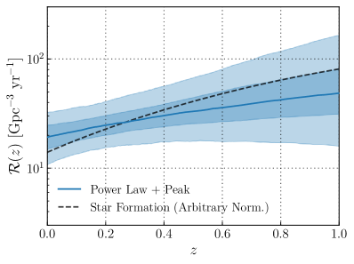
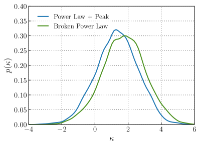
6 Conclusions
The publication of the second LIGO–Virgo gravitational-wave transient catalog has increased the population of BBH events by a factor of more than four. The new catalog has highlighted the limitations of some early population models while yielding remarkable new signatures:
-
1.
We find that the BBH primary mass spectrum is not well-described as a simple power-law with an abrupt cut-off; there is a strong statistical preference for other models with non-trivial features such as a peak or a tapering. These features occur at , where one might expect pair instability supernovae (and pulsational pair-instability supernovae) to shape the mass distribution of BHs.
-
2.
At the opposite end of the spectrum, we observe a dearth of systems between NS and BH masses, suggesting that the BH mass spectrum likely turns over at . We constrain the minimum mass of BHs in BBH systems to be at 90% credibility. This is greater than the mass of BH candidates in Galactic binaries, e.g., Thompson et al. (2019).
-
3.
Meanwhile, we find that our models This may indicate that \IfEqCaseGW190814AGW190413AGW190413_052954GW190719AGW190719_215514GW190620AGW190620_030421GW190514AGW190514_065416GW190731AGW190731_140936GW190503AGW190503_185404GW190602AGW190602_175927GW190929AGW190929_012149GW190517AGW190517_055101GW190915AGW190915_235702GW190425AGW190425GW190512AGW190512_180714GW190630AGW190630_185205GW190521AGW190521GW190413BGW190413_134308GW190924AGW190924_021846GW190930AGW190930_133541GW190706AGW190706_222641GW190408AGW190408_181802GW190909AGW190909_114149GW190728AGW190728_064510GW190426AGW190426_152155GW190412AGW190412GW190720AGW190720_000836GW190521BGW190521_074359GW190910AGW190910_112807GW190803AGW190803_022701GW190519AGW190519_153544GW190708AGW190708_232457GW190527AGW190527_092055GW190513AGW190513_205428GW190424AGW190424_180648GW190727AGW190727_060333GW190814AGW190814GW190707AGW190707_093326GW190828AGW190828_063405GW190828BGW190828_065509GW190701AGW190701_203306GW190421AGW190421_213856 belongs to a distinct population, or that there are additional features at the low mass end of the BBH mass spectrum that are missing in our models. This is perhaps unsurprising as the combination of mass ratio, merger rate, and secondary mass inferred from this system pose a challenge to our current understanding of compact binary formation (Abbott et al., 2020b; Arca Sedda, 2020b; Zevin et al., 2020; Safarzadeh, 2020).
-
4.
We detect clear evidence of spin-induced, general relativistic precession of the orbital plane. We determine that this signature is not due to a single precessing merger, but from the overall preference of the data for precessing waveforms.
-
5.
We observe that some fraction of the BHs in GWTC-2 are spinning with an orientation that is anti-aligned with respect to the orbital angular momentum of the binary. If we plausibly assume that all binaries with anti-aligned spins are assembled dynamically, this may imply that LIGO–Virgo events merge both dynamically and in the field. Based on the inferred mass and spin distributions, we find no clear evidence for or against hierarchical mergers in GWTC-2.
-
6.
We compute the rate of compact binary mergers, finding and . The data are consistent with both a merger rate that is constant in time and one that tracks the SFR in the local universe, though the data prefer a merger rate that is somewhere in between. We find that the merger rate at differs from the merger rate at by a factor of , to be compared with the SFR, .
While a clearer picture is emerging of the population properties of compact binaries, key questions remain. How do we best characterize the deviations from power-law in the primary BH mass spectrum, and what is the physical origin of these new features? What is the origin of BBH mergers in the high-mass gap: hierarchical mergers, stars producing remnants heavier than expected from pair instability supernovae theory, or something else? What is the shape of the mass spectrum between NS and BH masses, and does the current dearth of systems between and represent an empty low-mass gap? If so, do systems like the secondary mass of \IfEqCaseGW190814AGW190413AGW190413_052954GW190719AGW190719_215514GW190620AGW190620_030421GW190514AGW190514_065416GW190731AGW190731_140936GW190503AGW190503_185404GW190602AGW190602_175927GW190929AGW190929_012149GW190517AGW190517_055101GW190915AGW190915_235702GW190425AGW190425GW190512AGW190512_180714GW190630AGW190630_185205GW190521AGW190521GW190413BGW190413_134308GW190924AGW190924_021846GW190930AGW190930_133541GW190706AGW190706_222641GW190408AGW190408_181802GW190909AGW190909_114149GW190728AGW190728_064510GW190426AGW190426_152155GW190412AGW190412GW190720AGW190720_000836GW190521BGW190521_074359GW190910AGW190910_112807GW190803AGW190803_022701GW190519AGW190519_153544GW190708AGW190708_232457GW190527AGW190527_092055GW190513AGW190513_205428GW190424AGW190424_180648GW190727AGW190727_060333GW190814AGW190814GW190707AGW190707_093326GW190828AGW190828_063405GW190828BGW190828_065509GW190701AGW190701_203306GW190421AGW190421_213856 belong to the NS or BH side of the gap? Is the observation of anti-aligned spins indicative of dynamically assembled binaries? As the sensitivity of LIGO, Virgo, and KAGRA improves, and as more gravitational-wave transients are detected, we expect to begin to answer these questions.
References
- Aasi et al. (2015) Aasi, J., et al. 2015, CQGra, 32, 074001
- Abbott et al. (2013) Abbott, B., Abbott, R., Abbott, T., et al. 2013, Prospects for Observing and Localizing Gravitational-Wave Transients with Advanced LIGO, Advanced Virgo and KAGRA, arXiv:1304.0670
- Abbott et al. (2016a) —. 2016a, PhRvD, 94, 064035
- Abbott et al. (2016b) —. 2016b, PhRvL, 116, 241103
- Abbott et al. (2016c) —. 2016c, PhRvL, 116, 241102
- Abbott et al. (2019a) —. 2019a, ApJL, 882, L24
- Abbott et al. (2019b) —. 2019b, PhRvX, 9, 031040
- Abbott et al. (2019c) —. 2019c, arXiv:1912.11716
- Abbott et al. (2020a) Abbott, R., Abbott, T., Abraham, S., et al. 2020a, arXiv:2004.08342
- Abbott et al. (2020b) —. 2020b, ApJL, 896, L44
- Abbott et al. (2020c) —. 2020c, arXiv e-prints, arXiv:2010.14527
- Abbott et al. (2020d) Abbott, R., et al. 2020d
- Abbott et al. (2020e) —. 2020e, PhRvL, 125, 101102
- Abbott et al. (2020f) —. 2020f, ApJL, 900, L13
- Acernese et al. (2015) Acernese, F., et al. 2015, CQGra, 32, 024001
- Adams et al. (2016) Adams, T., Buskulic, D., Germain, V., et al. 2016, Classical and Quantum Gravity, 33, 175012
- Allen (2005) Allen, B. 2005, PhRvD, 71, "062001"
- Allen et al. (2012) Allen, B., Anderson, W. G., Brady, P. R., Brown, D. A., & Creighton, J. D. E. 2012, PhRvD, 85, "122006"
- Antonini & Gieles (2020) Antonini, F., & Gieles, M. 2020, arXiv e-prints, arXiv:2009.01861
- Antonini et al. (2014) Antonini, F., Murray, N., & Mikkola, S. 2014, ApJ, 781, 45
- Antonini & Rasio (2016) Antonini, F., & Rasio, F. A. 2016, ApJ, 831, 187
- Antonini et al. (2018) Antonini, F., Rodriguez, C. L., Petrovich, C., & Fischer, C. L. 2018, Mon. Not. R. Ast. Soc. Lett., 480, L58
- Antonini et al. (2017) Antonini, F., Toonen, S., & Hamers, A. S. 2017, ApJ, 841, 77
- Apostolatos et al. (1994) Apostolatos, T. A., Cutler, C., Sussman, G. J., & Thorne, K. S. 1994, PhRvD, 49, 6274
- Arca Sedda (2020a) Arca Sedda, M. 2020a, ApJ, 891, 47
- Arca Sedda (2020b) —. 2020b, Communications Physics, 3, 43
- Arca Sedda et al. (2020) Arca Sedda, M., Mapelli, M., Spera, M., Benacquista, M., & Giacobbo, N. 2020, ApJ, 894, 133
- Ashton & Thrane (2020) Ashton, G., & Thrane, E. 2020, Mon. Not. Roy. Astron. Soc., 498, 1905
- Ashton et al. (2019) Ashton, G., Hübner, M., Lasky, P. D., et al. 2019, ApJS, 241, 27
- Babak et al. (2017) Babak, S., Taracchini, A., & Buonanno, A. 2017, Phys. Rev. D, 95, 024010
- Baibhav et al. (2019) Baibhav, V., Berti, E., Gerosa, D., et al. 2019, PhRvD, 100, 064060
- Bailyn et al. (1998) Bailyn, C., Jain, R. K., Coppi, P., & Orosz, J. A. 1998, ApJ, 499, 367
- Banerjee et al. (2010) Banerjee, S., Baumgardt, H., & Kroupa, P. 2010, MNRAS, 402, 371
- Barkat et al. (1967) Barkat, Z., Rakavy, G., & Sack, N. 1967, PhRvL, 18, 379
- Bartos et al. (2017) Bartos, I., Kocsis, B., Haiman, Z., & Márka, S. 2017, ApJ, 835, 165
- Bavera et al. (2019) Bavera, S. S., Fragos, T., Qin, Y., et al. 2019, A&A, 635, A97
- Belczynski et al. (2002) Belczynski, K., Kalogera, V., & Bulik, T. 2002, ApJ, 572, 407
- Belczynski et al. (2016) Belczynski, K., Heger, A., Gladysz, W., et al. 2016, A&A, 594, A97
- Belczynski et al. (2020) Belczynski, K., Klencki, J., Fields, C. E., et al. 2020, A&A, 636, A104
- Berti & Volonteri (2008) Berti, E., & Volonteri, M. 2008, ApJ, 684, 822
- Bethe & Brown (1998) Bethe, H. A., & Brown, G. E. 1998, ApJ, 506, 780
- Biscoveanu et al. (2020) Biscoveanu, S., Isi, M., Vitale, S., & Varma, V. 2020, arXiv:2007.09156
- Bohé et al. (2016) Bohé, A., Hannam, M., Husa, S., et al. 2016
- Bohé et al. (2017) Bohé, A., et al. 2017, PhRvD, 95, 044028
- Calderón Bustillo et al. (2020) Calderón Bustillo, J., Sanchis-Gual, N., Torres-Forné, A., & Font, J. A. 2020, arxiv/2009.01066
- Calderón Bustillo et al. (2017) Calderón Bustillo, J., Laguna, P., & Shoemaker, D. 2017, Physical Review D, 95, doi:10.1103/physrevd.95.104038
- Canton et al. (2014) Canton, T. D., et al. 2014, PhRvD, 90, 082004
- Carlo et al. (2019a) Carlo, U. D., et al. 2019a, arxiv/1911.01434
- Carlo et al. (2019b) —. 2019b, MNRAS, 487, 2947
- Carpenter et al. (2017) Carpenter, B., Gelman, A., Hoffman, M. D., et al. 2017, Journal of Statistical Software, 76, doi:10.18637/jss.v076.i01
- Carr et al. (2016) Carr, B., Kühnel, F., & Sandstad, M. 2016, PhRvD, 94, 083504
- Carr & Hawking (1974) Carr, B. J., & Hawking, S. W. 1974, MNRAS, 168, 399
- Chatziioannou et al. (2019) Chatziioannou, K., et al. 2019, PhRvD, 100, 104015
- Chu (2017) Chu, Q. 2017, PhD thesis, The University of Western Australia
- Croon et al. (2020) Croon, D., McDermott, S. D., & Sakstein, J. 2020, arXiv:2007.07889
- Dai et al. (2017) Dai, L., Venumadhav, T., & Sigurdson, K. 2017, PhRvD, D95, 044011
- Damour (2001) Damour, T. 2001, PhRvD, 64, 124013
- de Mink & Mandel (2016) de Mink, S. E., & Mandel, I. 2016, MNRAS, 460, 3545
- Doctor et al. (2019) Doctor, Z., Wysocki, D., O’Shaughnessy, R., Holz, D. E., & Farr, B. 2019, ApJ, 893, 35
- Dominik et al. (2013) Dominik, M., Belczynski, K., Fryer, C., et al. 2013, ApJ, 779, 72
- Dominik et al. (2015) Dominik, M., Berti, E., O’Shaughnessy, R., et al. 2015, apj, 806, 263
- Downing et al. (2011) Downing, J. M. B., Benacquista, M. J., Giersz, M., & Spurzem, R. 2011, MNRAS, 416, 133
- Eldridge et al. (2019) Eldridge, J. J., Stanway, E. R., & Tang, P. N. 2019, MNRAS, 482, 870
- Eldridge et al. (2017) Eldridge, J. J., Stanway, E. R., Xiao, L., et al. 2017, PASA, 34, e058
- Essick & Landry (2020) Essick, R., & Landry, P. 2020, arXiv:2007.01372
- Fairhurst et al. (2019) Fairhurst, S., Green, R., Hannam, M., & Hoy, C. 2019, arXiv:1908.00555
- Farmer et al. (2020) Farmer, R., Renzo, M., de Mink, S., Fishbach, M., & Justham, S. 2020, arXiv e-prints, arXiv:2006.06678
- Farmer et al. (2019) Farmer, R., Renzo, M., de Mink, S. E., Marchant, P., & Justham, S. 2019, ApJ, 887, 53
- Farr et al. (2018) Farr, B., Holz, D. E., & Farr, W. M. 2018, ApJL, 854, L9
- Farr (2019) Farr, W. M. 2019, Research Notes of the American Astronomical Society, 3, 66
- Farr et al. (2011) Farr, W. M., Sravan, N., Cantrell, A., et al. 2011, ApJ, 741, 103
- Farr et al. (2017) Farr, W. M., Stevenson, S., Coleman Miller, M., et al. 2017, Nature, 548, 426
- Farrell et al. (2020) Farrell, E. J., Groh, J. H., Hirschi, R., et al. 2020, arXiv:2009.06585
- Farrow et al. (2019) Farrow, N., Zhu, X.-J., & Thrane, E. 2019, ApJ, 876, 18
- Fernandez & Profumo (2019) Fernandez, N., & Profumo, S. 2019, J. Cosmology Astropart. Phys, 2019, 022
- Fishbach et al. (2020a) Fishbach, M., Essick, R., & Holz, D. E. 2020a, arXiv:2006.13178
- Fishbach et al. (2020b) Fishbach, M., Farr, W. M., & Holz, D. E. 2020b, ApJL, 891, L31
- Fishbach & Holz (2017) Fishbach, M., & Holz, D. E. 2017, ApJL, 851, L25
- Fishbach & Holz (2020a) Fishbach, M., & Holz, D. E. 2020a, ApJ, 904, L26
- Fishbach & Holz (2020b) —. 2020b, ApJL, 891, L27
- Fishbach et al. (2017) Fishbach, M., Holz, D. E., & Farr, B. 2017, ApJL, 840, L24
- Fishbach et al. (2018) Fishbach, M., Holz, D. E., & Farr, W. M. 2018, ApJL, 863, L41
- Foreman-Mackey et al. (2013) Foreman-Mackey, D., Hogg, D. W., Lang, D., & Goodman, J. 2013, Publ. Astron. Soc. Pac, 125, 306
- Fowler & Hoyle (1964) Fowler, W. A., & Hoyle, F. 1964, ApJS, 9, 201
- Fragione et al. (2019) Fragione, G., Grishin, E., Leigh, N. W. C., Perets, H. B., & Perna, R. 2019, MNRAS, 488, 47
- Fragione & Kocsis (2018) Fragione, G., & Kocsis, B. 2018, Phys. Rev. Lett., 121, 161103
- Fragione & Kocsis (2019) —. 2019, MNRAS, 486, 4781
- Fragione & Kocsis (2020) —. 2020, MNRAS, 493, 3920
- Fuller & Ma (2019) Fuller, J., & Ma, L. 2019, ApJL, 881, L1
- Fuller et al. (2019) Fuller, J., Piro, A. L., & Jermyn, A. S. 2019, MNRAS, 485, 3661
- Galaudage et al. (2020) Galaudage, S., Adamcewicz, C., Zhu, X.-J., & Thrane, E. 2020, arxiv/2011.01495
- Galaudage et al. (2019) Galaudage, S., Talbot, C., & Thrane, E. 2019, arxiv/1912.09708
- Gayathri et al. (2020) Gayathri, V., Healy, J., Lange, J., et al. 2020, arxiv/2009.05461
- Gerosa & Berti (2017) Gerosa, D., & Berti, E. 2017, PhRvD, 95, 124046
- Gerosa et al. (2018) Gerosa, D., Berti, E., O’Shaughnessy, R., et al. 2018, PhRvD, 98, 084036
- Giacobbo et al. (2017) Giacobbo, N., Mapelli, M., & Spera, M. 2017, MNRAS, 474, 2959
- Gröbner et al. (2020) Gröbner, M., Ishibashi, W., Tiwari, S., Haney, M., & Jetzer, P. 2020, A&A, 638, A119
- Gültekin et al. (2004) Gültekin, K., Miller, M. C., & Hamilton, D. P. 2004, ApJ, 616, 221
- Hanna et al. (2020) Hanna, C., et al. 2020, PhRvD, 101, 022003
- Hannam et al. (2014) Hannam, M., et al. 2014, PhRvL, 113, 151101
- Hannuksela et al. (2019) Hannuksela, O. A., Haris, K., Ng, K. K. Y., et al. 2019, ApJ, 874, L2
- Harry et al. (2016) Harry, I., Privitera, S., Bohé, A., & Buonanno, A. 2016, Physical Review D, 94, doi:10.1103/physrevd.94.024012
- Heger et al. (2003) Heger, A., Fryer, C. L., Woosley, S. E., Langer, N., & Hartmann, D. H. 2003, ApJ, 591, 288
- Heger & Woosley (2002) Heger, A., & Woosley, S. E. 2002, ApJ, 567, 532
- Huang et al. (2020) Huang, Y., Haster, C.-J., Vitale, S., et al. 2020, arXiv e-prints, arXiv:2003.04513
- Husa et al. (2016) Husa, S., et al. 2016, PhRvD, 93, 044006
- Inayoshi et al. (2017) Inayoshi, K., Hirai, R., Kinugawa, T., & Hotokezaka, K. 2017, Mon. Not. Roy. Astron. Soc., 468, 5020
- Jeffreys (1961) Jeffreys, H. 1961, Theory of Probability, 3rd edn. (Oxford University Press)
- Kalogera (2000) Kalogera, V. 2000, apj, 541, 319
- Khan et al. (2020) Khan, S., Ohme, F., Chatziioannou, K., & Hannam, M. 2020, PhRvD, 101, 024056
- Khan et al. (2016) Khan, S., et al. 2016, PhRvD, 93, 044007
- Kidder (1995) Kidder, L. E. 1995, Phys. Rev. D, 52, 821
- Kimball et al. (2020a) Kimball, C., Talbot, C., Berry, C. P., et al. 2020a, ApJ, 900, 177
- Kimball et al. (2020b) —. 2020b, arxiv/2011.05332
- Kimpson et al. (2016) Kimpson, T. O., Spera, M., Mapelli, M., & Ziosi, B. M. 2016, MNRAS, 463, 2443
- Klimenko & Mitselmakher (2004) Klimenko, S., & Mitselmakher, G. 2004, Class. Quant. Grav., 21, S1819
- Klimenko et al. (2016) Klimenko, S., et al. 2016, PhRvD, 93, 042004
- Kopparapu et al. (2008) Kopparapu, R. K., Hanna, C., Kalogera, V., et al. 2008, apj, 675, 1459
- Kovetz et al. (2017) Kovetz, E. D., Cholis, I., Breysse, P. C., & Kamionkowski, M. 2017, PhRvD, 95, 103010
- Kreidberg et al. (2012) Kreidberg, L., Bailyn, C. D., Farr, W. M., & Kalogera, V. 2012, ApJ, 757, 36
- Kulkarni et al. (1993) Kulkarni, S. R., Hut, P., & McMillan, S. 1993, Nature, 364, 421
- Kushnir et al. (2016) Kushnir, D., Zaldarriaga, M., Kollmeier, J. A., & Waldman, R. 2016, MNRAS, 462, 844
- Lange et al. (2018) Lange, J., O’Shaughnessy, R., & Rizzo, M. 2018, arxiv/1805.10457
- Li et al. (2018) Li, S.-S., Mao, S., Zhao, Y., & Lu, Y. 2018, MNRAS, 476, 2220
- LIGO Scientific Collaboration (2018) LIGO Scientific Collaboration. 2018, LIGO Algorithm Library - LALSuite, Free Software (GPL), doi:10.7935/GT1W-FZ16
- LIGO-Virgo (2020) LIGO-Virgo. 2020, GWTC-2 Data Release: Sensitivity of Matched Filter Searches to Binary Black Hole Merger Populations, doi:https://dcc.ligo.org/LIGO-P2000217/public
- Liu & Bromm (2020) Liu, B., & Bromm, V. 2020, arXiv e-prints, arXiv:2009.11447
- Liu et al. (2019) Liu, B., Lai, D., & Wang, Y.-H. 2019, ApJ, 881, 41
- Loredo (2004) Loredo, T. J. 2004, in American Institute of Physics Conference Series, Vol. 735, 195–206
- Lower et al. (2018) Lower, M. E., Thrane, E., Lasky, P. D., & Smith, R. J. E. 2018, PhRvD, 98, 083028
- Madau & Dickinson (2014) Madau, P., & Dickinson, M. 2014, Annual Review of Astronomy and Astrophysics, 52, 415
- Madau & Rees (2001) Madau, P., & Rees, M. J. 2001, ApJL, 551, L27
- Magee et al. (2019) Magee, R., et al. 2019, ApJ, 878, L17
- Mandel & de Mink (2016) Mandel, I., & de Mink, S. E. 2016, MNRAS, 458, 2634
- Mandel et al. (2019) Mandel, I., Farr, W. M., & Gair, J. R. 2019, MNRAS, 486, 1086
- Mandel et al. (2021) Mandel, I., Müller, B., Riley, J., et al. 2021, MNRAS, 500, 1380
- Mandel & O’Shaughnessy (2010) Mandel, I., & O’Shaughnessy, R. 2010, CQGra, 27, 114007
- Mapelli (2016) Mapelli, M. 2016, MNRAS, 459, 3432
- Mapelli et al. (2017) Mapelli, M., Giacobbo, N., Ripamonti, E., & Spera, M. 2017, MNRAS, 472, 2422
- Mapelli et al. (2020) Mapelli, M., Spera, M., Montanari, E., et al. 2020, ApJ, 888, 76
- Marchant et al. (2016) Marchant, P., Langer, N., Podsiadlowski, P., Tauris, T. M., & Moriya, T. J. 2016, A&A, 588, A50
- Marchant & Moriya (2020) Marchant, P., & Moriya, T. 2020, arXiv:2007.06220
- McKernan et al. (2012) McKernan, B., Ford, K. E. S., Lyra, W., & Perets, H. B. 2012, MNRAS, 425, 460
- McKernan et al. (2020) McKernan, B., Ford, K. E. S., O’Shaughnessy, R., & Wysocki, D. 2020, MNRAS, 494, 1203
- McKernan et al. (2018) McKernan, B., Saavik Ford, K. E., Bellovary, J., et al. 2018, ApJ, 866, 66
- Messick et al. (2017) Messick, C., et al. 2017, PhRvD, 95, 042001
- Miller & Hamilton (2002a) Miller, C. M., & Hamilton, D. P. 2002a, ApJ, 576, 894
- Miller & Hamilton (2002b) Miller, M. C., & Hamilton, D. P. 2002b, MNRAS, 330, 232
- Miller & Lauburg (2009) Miller, M. C., & Lauburg, V. M. 2009, ApJ, 692, 917
- Miller et al. (2020) Miller, S., Callister, T. A., & Farr, W. 2020, ApJ, 895, 128
- Moody & Sigurdsson (2009) Moody, K., & Sigurdsson, S. 2009, ApJ, 690, 1370
- Most et al. (2020) Most, E. R., Papenfort, L. J., Weih, L. R., & Rezzolla, L. 2020, arXiv:2006.14601
- Natarajan (2020) Natarajan, P. 2020, arXiv e-prints, arXiv:2009.09156
- Neijssel et al. (2019) Neijssel, C. J., Vigna-Gómez, A., Stevenson, S., et al. 2019, MNRAS, 490, 3740
- Ng et al. (2018a) Ng, K. K., Vitale, S., Zimmerman, A., et al. 2018a, PhRvD, 98, 083007
- Ng et al. (2018b) Ng, K. K. Y., Wong, K. W. K., Broadhurst, T., & Li, T. G. F. 2018b, PhRvD, 97, 023012
- Nitz et al. (2019a) Nitz, A., et al. 2019a, "gwastro/pycbc: Pycbc release v1.15.0”
- Nitz et al. (2019b) Nitz, A. H., Capano, C., Nielsen, A. B., et al. 2019b, ApJ, 872, 195
- Nitz & Capano (2020) Nitz, A. H., & Capano, C. D. 2020, arxiv/2010.12558
- Nitz et al. (2017) Nitz, A. H., Dent, T., Canton, T. D., Fairhurst, S., & Brown", D. A. 2017, ApJ, 849, 118
- Nitz et al. (2020) Nitz, A. H., Dent, T., Davies, G. S., et al. 2020, ApJ, 891, 123
- Oguri (2018) Oguri, M. 2018, MNRAS, 3842
- O’Leary et al. (2009) O’Leary, R. M., Kocsis, B., & Loeb, A. 2009, MNRAS, 395, 2127
- O’Leary et al. (2006) O’Leary, R. M., Rasio, F. A., Fregeau, J. M., Ivanova, N., & O’Shaughnessy, R. 2006, ApJ, 637, 937
- Olejak et al. (2020) Olejak, A., Fishbach, M., Belczynski, K., et al. 2020, arXiv e-prints, arXiv:2004.11866
- O’Shaughnessy et al. (2017) O’Shaughnessy, R., Gerosa, D., & Wysocki, D. 2017, PhRvL, 119, 011101
- Ossokine et al. (2020) Ossokine, S., et al. 2020, arXiv:2004.09442
- Özel et al. (2011) Özel, F., Psaltis, D., Narayan, R., & McClintock, J. E. 2011, ApJ, 725, 1918
- Pan et al. (2014) Pan, Y., Buonanno, A., Taracchini, A., et al. 2014, Phys. Rev. D, 89, 084006
- Park et al. (2017) Park, D., Kim, C., Lee, H. M., Bae, Y.-B., & Belczynski, K. 2017, MNRAS, 469, 4665
- Portegies Zwart & McMillan (2000) Portegies Zwart, S. F., & McMillan, S. L. W. 2000, ApJ, 528, L17
- Portegies Zwart & Yungelson (1998) Portegies Zwart, S. F., & Yungelson, L. R. 1998, A&A, 332, 173
- Pratten & Vecchio (2020) Pratten, G., & Vecchio, A. 2020, arXiv:2008.00509
- Pretorius (2005) Pretorius, F. 2005, PhRvL, 95, 121101
- Qin et al. (2018) Qin, Y., Fragos, T., Meynet, G., et al. 2018, A&A, 616, A28
- Rice & Zhang (2020) Rice, J. R., & Zhang, B. 2020, arXiv e-prints, arXiv:2009.11326
- Riddell et al. (2018) Riddell, A., Hartikainen, A., Lee, D., Riddell-Stan, et al. 2018, Stan-Dev/Pystan: V2.18.0.0, doi:10.5281/ZENODO.1456206
- Rodriguez et al. (2018) Rodriguez, C. L., Amaro-Seoane, P., Chatterjee, S., & Rasio, F. A. 2018, PhRvL, 120, 151101
- Rodriguez & Antonini (2018) Rodriguez, C. L., & Antonini, F. 2018, ApJ, 863, 7
- Rodriguez & Loeb (2018) Rodriguez, C. L., & Loeb, A. 2018, ApJ, 866, L5
- Rodriguez et al. (2015) Rodriguez, C. L., Morscher, M., Pattabiraman, B., et al. 2015, Phys. Rev. Lett., 115, 051101
- Rodriguez et al. (2019) Rodriguez, C. L., Zevin, M., Amaro-Seoane, P., et al. 2019, PhRvD, 100, 043027
- Rodriguez et al. (2016) Rodriguez, C. L., Zevin, M., Pankow, C., Kalogera, V., & Rasio, F. A. 2016, ApJL, 832, L2
- Romero-Shaw et al. (2019) Romero-Shaw, I. M., Lasky, P. D., & Thrane, E. 2019, MNRAS, 490, 5210
- Romero-Shaw et al. (2020a) Romero-Shaw, I. M., Lasky, P. D., Thrane, E., & Bustillo, J. C. 2020a, ApJL, 903, L5
- Romero-Shaw et al. (2020b) Romero-Shaw, I. M., et al. 2020b, arxiv/2006.00714
- Roulet et al. (2020) Roulet, J., Venumadhav, T., Zackay, B., Dai, L., & Zaldarriaga, M. 2020, arXiv e-prints, arXiv:2008.07014
- Roulet & Zaldarriaga (2019) Roulet, J., & Zaldarriaga, M. 2019, MNRAS, 484, 4216
- Roupas & Kazanas (2019) Roupas, Z., & Kazanas, D. 2019, A&A, 632, L8
- Sachdev et al. (2019) Sachdev, S., et al. 2019, arXiv:1901.08580
- Safarzadeh (2020) Safarzadeh, M. 2020, Nature Astronomy, 4, 735
- Safarzadeh et al. (2020) Safarzadeh, M., Farr, W. M., & Ramirez-Ruiz, E. 2020, ApJ, 894, 129
- Safarzadeh & Haiman (2020) Safarzadeh, M., & Haiman, Z. 2020, arXiv e-prints, arXiv:2009.09320
- Samsing (2018) Samsing, J. 2018, PhRvD, 97, 103014
- Samsing et al. (2014) Samsing, J., MacLeod, M., & Ramirez-Ruiz, E. 2014, ApJ, 784, 71
- Samsing & Ramirez-Ruiz (2017) Samsing, J., & Ramirez-Ruiz, E. 2017, ApJL, 840, L14
- Santoliquido et al. (2020) Santoliquido, F., Mapelli, M., Bouffanais, Y., et al. 2020, arXiv e-prints, arXiv:2004.09533
- Schmidt et al. (2012) Schmidt, P., Hannam, M., & Husa, S. 2012, PhRvD, 86, 104063
- Schmidt et al. (2015) Schmidt, P., Ohme, F., & Hannam, M. 2015, PhRvD, 91, 024043
- Sigurdsson & Hernquist (1993) Sigurdsson, S., & Hernquist, L. 1993, Nature, 364, 423
- Smith et al. (2018) Smith, G. P., Jauzac, M., Veitch, J., et al. 2018, MNRAS, 475, 3823
- Speagle (2020) Speagle, J. S. 2020, MNRAS, 493, 3132
- Spera & Mapelli (2017) Spera, M., & Mapelli, M. 2017, MNRAS, 470, 4739
- Stevenson et al. (2017) Stevenson, S., Berry, C. P. L., & Mandel, I. 2017, MNRAS, 471, 2801
- Stone et al. (2017) Stone, N. C., Metzger, B. D., & Haiman, Z. 2017, MNRAS, 464, 946
- Sun et al. (2020) Sun, L., Goetz, E., Kissel, J. S., et al. 2020, Classical and Quantum Gravity, 37, 225008
- Tagawa et al. (2020) Tagawa, H., Haiman, Z., & Kocsis, B. 2020, The Astrophysical Journal, 898, 25
- Talbot et al. (2019) Talbot, C., Smith, R., Thrane, E., & Poole, G. B. 2019, PhRvD, 100, 043030
- Talbot & Thrane (2017) Talbot, C., & Thrane, E. 2017, PhRvD, 96, 023012
- Talbot & Thrane (2018) —. 2018, ApJ, 856, 173
- Tan et al. (2020) Tan, H., Noronha-Hostler, J., & Yunes, N. 2020, arXiv:2006.16296
- Tanikawa et al. (2020) Tanikawa, A., Susa, H., Yoshida, T., Trani, A. A., & Kinugawa, T. 2020, arXiv e-prints, arXiv:2008.01890
- Taracchini et al. (2014) Taracchini, A., et al. 2014, Phys. Rev. D, 89, 061502
- Tews et al. (2020) Tews, I., Pang, P. T., Dietrich, T., et al. 2020, arXiv:2007.06057
- Thompson et al. (2019) Thompson, T. A., et al. 2019, Science, 366
- Thrane & Talbot (2019) Thrane, E., & Talbot, C. 2019, PASA, 36, E010
- Tiwari (2018) Tiwari, V. 2018, Classical and Quantum Gravity, 35, 145009
- Tiwari (2020) —. 2020, arXiv e-prints, arXiv:2006.15047
- Tiwari et al. (2018) Tiwari, V., Fairhurst, S., & Hannam, M. 2018, ApJ, 868, 140
- Trovato et al. (2020) Trovato, A., et al. 2020, PoS, Asterics2019, 082
- Usman et al. (2016) Usman, S. A., et al. 2016, CQGra, 33, 215004
- van Son et al. (2020) van Son, L. A. C., de Mink, S. E., Broekgaarden, F. S., et al. 2020, arXiv e-prints, arXiv:2004.05187
- Varma et al. (2019) Varma, V., Field, S. E., Scheel, M. A., et al. 2019, Phys. Rev. Research, 1, 033015
- Veitch et al. (2015) Veitch, J., Raymond, V., Farr, B., et al. 2015, PhRvD, 91, 042003
- Venumadhav et al. (2019) Venumadhav, T., Zackay, B., Roulet, J., Dai, L., & Zaldarriaga, M. 2019, PhRvD, 100, 023011
- Venumadhav et al. (2020) —. 2020, PhRvD, 101, 083030
- Vigna-Gómez et al. (2020) Vigna-Gómez, A., Toonen, S., Ramirez-Ruiz, E., et al. 2020, arXiv e-prints, arXiv:2010.13669
- Vitale (2020) Vitale, S. 2020, arXiv:2007.05579
- Vitale et al. (2017a) Vitale, S., Gerosa, D., Haster, C.-J., Chatziioannou, K., & Zimmerman, A. 2017a, PhRvL, 119, 251103
- Vitale et al. (2017b) Vitale, S., Lynch, R., Sturani, R., & Graff, P. 2017b, Class. Quant. Grav., 34, 03LT01
- Woosley (2017) Woosley, S. E. 2017, ApJ, 836, 244
- Woosley & Heger (2015) Woosley, S. E., & Heger, A. 2015, in Very Massive Stars Local Universe (Springer, Cham), 199–225
- Woosley et al. (2002) Woosley, S. E., Heger, A., & Weaver, T. A. 2002, Rev. of Mod. Phys., 74, 1015
- Wysocki (2020) Wysocki, D. 2020
- Wysocki et al. (2019a) Wysocki, D., Lange, J., & O’Shaughnessy, R. 2019a, PhRvD, 100, 043012
- Wysocki & O’Shaughnessy (2017) Wysocki, D., & O’Shaughnessy, R. 2017, Bayesian Parametric Population Models, bayesian-parametric-population-models.readthedocs.io
- Wysocki et al. (2019b) Wysocki, D., O’Shaughnessy, R., Lange, J., & Fang, Y.-L. L. 2019b, PhRvD, 99
- Wysocki et al. (2018) Wysocki, D., et al. 2018, PhRvD, 97, 043014
- Yang et al. (2019) Yang, Y., Bartos, I., Gayathri, V., et al. 2019, PhRvL, 123, 181101
- Zackay et al. (2020) Zackay, B., Dai, L., Venumadhav, T., Roulet, J., & Zaldarriaga, M. 2020, PhRvD, 101, 083030
- Zackay et al. (2019) Zackay, B., Venumadhav, T., Dai, L., Roulet, J., & Zaldarriaga, M. 2019, PhRvD, 100, 023007
- Zaldarriaga et al. (2018) Zaldarriaga, M., Kushnir, D., & Kollmeier, J. A. 2018, MNRAS, 473, 4174
- Zevin et al. (2017) Zevin, M., Pankow, C., Rodriguez, C. L., et al. 2017, ApJ, 846, 82
- Zevin et al. (2019) Zevin, M., Samsing, J., Rodriguez, C., Haster, C.-J., & Ramirez-Ruiz, E. 2019, ApJ, 871, 91
- Zevin et al. (2020) Zevin, M., Spera, M., Berry, C. P., & Kalogera, V. 2020, arXiv:2006.14573
- Zhang & Li (2020) Zhang, N.-B., & Li, B.-A. 2020, arXiv:2007.02513
- Ziegler & Freese (2020) Ziegler, J., & Freese, K. 2020, arXiv e-prints, arXiv:2010.00254
- Ziosi et al. (2014) Ziosi, B. M., Mapelli, M., Branchesi, M., & Tormen, G. 2014, MNRAS, 441, 3703
Appendix A Estimating the detection fraction
A key ingredient in Eqs. (1) and (2) is the detection fraction , the fraction of systems within some prior volume (redshift ) that we expect to successfully detect. The detection fraction quantifies selection biases, and so it is critical to accurately characterize. For a population described by hyper-parameters , the detection fraction is
| (A1) |
Here, is the detection probability: the probability that an event with parameters is detectable. The detection probability depends primarily on the masses and redshift of a system, and, to a lesser degree, on the spins.
We calculate using injections. We simulate compact binary signals from a reference population and record which ones are successfully detected by the PyCBC and GstLAL search pipelines; see Abbott et al. (2020c). Following Tiwari (2018); Farr (2019); Vitale (2020); Loredo (2004), the point estimate for Eq. A1 is calculated using a Monte Carlo integral over found injections:
| (A2) |
where is the total number of injections, are the injections that are successfully detected, and is the probability distribution from which the injections are drawn; see LIGO-Virgo (2020) for additional details. When sampling the population likelihood, we marginalize over the uncertainty in following Farr (2019), and ensure that the effective number of found injections remaining after population re-weighting is sufficiently high ().
For the O3a observing period, we use the injection campaign described in Abbott et al. (2020c) and characterize the found injections as those recovered with a FAR below our threshold of in either PyCBC or GstLAL. For the O1 and O2 observing period, we supplement the O3a pipeline injections with mock injections drawn from the same distribution above. For the mock injections, we calculate according to the semi-analytic approximation described in Abbott et al. (2019a), based on a single-detector signal-to-noise ratio threshold and the Advanced LIGO Early-High Noise PSD (Abbott et al., 2013). We combine O1, O2 and O3 injection sets ensuring a constant rate of injections across the total observing time, yielding injections for O3a and for O1 and O2. To control computational costs, not all of the injections are performed in real data. Before injecting, the expected network signal-to-noise ratio of the injections is computed, and the hopeless injections with signal-to-noise ratio are removed.
Due to the finite number of injections, we approximate Eq. (A1) with a fixed spin distribution instead of the distribution implied by . When combining the Truncated, Power Law + Peak, Broken Power Law and Multi Peak mass models together with the Default spin distribution, we assume that the aligned spin components are independently drawn from a uniform distribution . By making this approximation, we are in effect ignoring selection effects due to spin. Nevertheless, we expect this approximation to have a negligible impact on the inferred spin distribution compared to the statistical uncertainties. For aligned spin components in the range , the detection probability varies by no more than a factor of 2 (Ng et al., 2018a). Furthermore, our main conclusions regarding the spin distribution inferred from the Default model are supported by the Gaussian model, which requires no approximations for spin selection effects. The Multi Spin model calculates Eq. (A1) by calibrating a semi-analytic approximation to the list of found injections (Wysocki, 2020).
Appendix B Details of mass population models
In this section we provide details about the population models described above in Section 3; see also Fig. 1. Each subsection includes a table with a summary of the parameters for that model and the prior distribution used for each parameter. The prior distributions are indicated using abbreviations: for example, translates to uniform on the interval and LU() translates to log-uniform on the interval .
B.1 Truncated mass model
This model is equivalent to “Model B” in Abbott et al. (2019a). The primary mass distribution for this model follows a power-law with spectral index , and with a sharp cut-off at the lower end and the upper end of the distribution :
| (B1) |
Meanwhile, the mass ratio follows a power-law distribution with spectral index
| (B2) |
The hyper-parameters for this model are summarized in Table 5.
| Parameter | Description | Prior | |
|---|---|---|---|
| Spectral index for the power-law of the primary mass distribution. | U(, ) | ||
| Spectral index for the power-law of the mass ratio distribution. | U(, ) | ||
| Minimum mass of the power-law component of the primary mass distribution. | U(, ) | ||
| Maximum mass of the power-law component of the primary mass distribution. | U(, ) |
B.2 Power Law + Peak mass model
This is equivalent to “Model C” from Abbott et al. (2019a). It is motivated by the idea that the mass loss undergone by pulsational pair-instability supernovae could lead to a pile-up of BBH events before the pair-instability gap (Talbot & Thrane, 2018). The primary mass distribution is an extension of Truncated with the addition of tapering at the lower mass end of the distribution and a Gaussian component:
| (B3) |
Here, is a normalized power-law distribution with spectral index and high-mass cut-off . Meanwhile, is a normalized Gaussian distribution with mean and width . The parameter is a mixing fraction determining the relative prevalence of mergers in and . Finally, is a smoothing function, which rises from 0 to 1 over the interval :
| (B4) |
with
| (B5) |
The conditional mass ratio distribution in this model also includes the smoothing term:
| (B6) |
The hyper-parameters for this model are summarized in Table 6.
In Fig. 16, we provide a corner plot representation of the posterior distribution for the Power Law + Peak hyper-parameters. The panel describes the Gaussian component: is the center of the Gaussian while is the fraction of mergers taking place in the Gaussian (as opposed to the power-law distribution). Judging from this panel, it appears at first that peaks close to (corresponding to no Gaussian peak). However, if we zoom in as in Fig. 6, we see that the posterior for is peaked clearly away from zero at . This is consistent with the large Bayes factor indicating preference for Power Law + Peak over Truncated.
| Parameter | Description | Prior | |
|---|---|---|---|
| Spectral index for the power-law of the primary mass distribution. | U(, ) | ||
| Spectral index for the power-law of the mass ratio distribution. | U(, ) | ||
| Minimum mass of the power-law component of the primary mass distribution. | U(, ) | ||
| Maximum mass of the power-law component of the primary mass distribution. | U(, ) | ||
| Fraction of BBH systems in the Gaussian component. | U(0, 1) | ||
| Mean of the Gaussian component in the primary mass distribution. | U(, ) | ||
| Width of the Gaussian component in the primary mass distribution. | U(, ) | ||
| Range of mass tapering at the lower end of the mass distribution. | U(, ) |
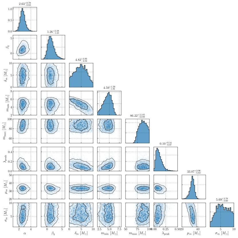
B.3 Broken Power Law mass model
This model is an extension of Truncated. The primary mass distribution consists of a broken power-law. This is motivated by the potential tapering of the primary mass distribution at high masses. Also, the model employs a smoothing function to prevent a sharp cut-off at low masses.
| (B7) |
Here,
| (B8) |
is the mass where there is a break in the spectral index and is the fraction of the way between and at which the primary mass distribution undergoes a break. Meanwhile, is a smoothing function as in Eq. (B4). The conditional mass ratio distribution is the same as in the Power Law + Peak model; see Eq. B6. The hyper-parameters for this model are summarized in Table 7. In Fig. 17 we provide a corner plot for Broken Power Law. In the limit of no low-mass smoothing (), and in the limit of a second power-law with a steep slope that mimics a sharp cutoff (), this model reduces to Truncated. Above, we noted that the Broken Power Law model prefers a break in the primary mass spectrum near . On the other hand, if we believe that the feature represented by should be closer to a sharp cutoff, then the cut-off must occur at higher masses approaching the maximum mass of Truncated at . This can be seen by the correlation between and in Fig. 17.
| Parameter | Description | Prior | |
|---|---|---|---|
| Power-law slope of the primary mass distribution for masses below . | U(, ) | ||
| Power-law slope for the primary mass distribution for masses above . | U(, ) | ||
| Spectral index for the power-law of the mass ratio distribution. | U(, ) | ||
| Minimum mass of the power-law component of the primary mass distribution. | U(, ) | ||
| Maximum mass of the primary mass distribution. | U(, ) | ||
| The fraction of the way between and at which the primary mass distribution breaks, e.g. a break fraction of 0.4 between and means the break occurs at . | U(0, 1) | ||
| Range of mass tapering on the lower end of the mass distribution. | U(, ) |
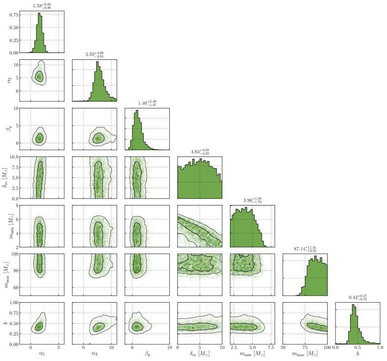
B.4 Multi Peak mass model
This model in an extension of Power Law + Peak, where there is an additional Gaussian component at the upper end of the mass distribution motivated by a possible subpopulation of objects in the upper mass gap:
| (B9) |
Here, the parameters and correspond to the fraction of binaries in any Gaussian component and the fraction of binaries in the lower-mass Gaussian of the Gaussian components, respectively. The distribution is a normalized Gaussian distribution for the lower-mass peak with mean and width and is a normalized Gaussian distribution for the upper-mass peak with mean and width . The hyper-parameters for this model are summarized in Table 8. In Fig. 19, we provide a posterior predictive check for all of the mass models used in this analysis.
| Parameter | Description | Prior | |
|---|---|---|---|
| Spectral index for the power-law of the primary mass distribution. | U(, ) | ||
| Spectral index for the power-law of the mass ratio distribution. | U(, ) | ||
| Minimum mass of the power-law component of the primary mass distribution. | U(, ) | ||
| Maximum mass of the power-law component of the primary mass distribution. | U(, ) | ||
| Fraction of BBH systems in the Gaussian components. | U(0, 1) | ||
| Fraction of BBH systems iin the Gaussian components belonging to the lower-mass component. | U(0, 1) | ||
| Mean of the lower-mass Gaussian component in the primary mass distribution. | U(, ) | ||
| Width of the lower-mass Gaussian component in the primary mass distribution. | U(, ) | ||
| Mean of the upper-mass Gaussian component in the primary mass distribution. | U(, ) | ||
| Width of the upper-mass Gaussian component in the primary mass distribution. | U(, ) | ||
| Range of mass tapering on the lower end of the mass distribution. | U(, ) |
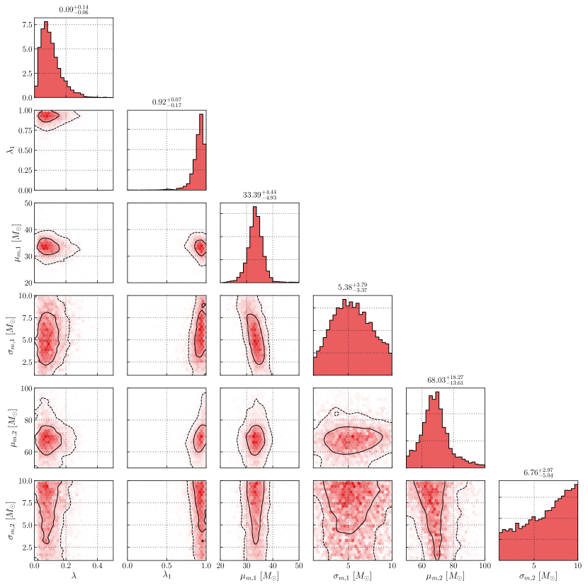
Appendix C Mass Model Checking
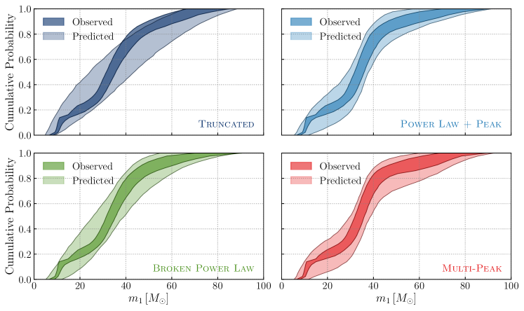
Section 5.1 describes the inferred mass distribution obtained with the Truncated, Broken Power Law, Power Law + Peak, and Multi Peak models, and compares the different models by calculating their Bayes factors. Here we assess the goodness-of-fit of the models using posterior predictive checks, comparing predicted and empirical catalogs of observed distributions in Fig. 19. The light colored bands show the cumulative distribution of as predicted by the model, while the darker bands show the empirical distribution based on the actual events observed in GWTC-2. The bands represent a family of curves, where each curve corresponds to a different draw from the population hyper-posterior. Each draw from the hyper-posterior updates both the predicted distribution (in the lighter color) and the empirical distribution (in the darker color), as the individual event posteriors are updated according to the inferred population distribution (Fishbach et al., 2020b; Galaudage et al., 2019; Miller et al., 2020). If the model is a good fit to the data, the dark colored bands should overlap with the light colored bands. Figure 19 shows the relatively poor fit for the Truncated model, which cannot capture the excess of events at – compared to . The remaining panels show the improved fits with the Power Law + Peak, Broken Power Law and Multi Peak models. These results are consistent with the Bayes factors in Table 2, which conclude that the Truncated model is disfavored by a Bayes factor of 10–80 relative to the other models.
C.1 On GW190412
Other than \IfEqCaseGW190814AGW190413AGW190413_052954GW190719AGW190719_215514GW190620AGW190620_030421GW190514AGW190514_065416GW190731AGW190731_140936GW190503AGW190503_185404GW190602AGW190602_175927GW190929AGW190929_012149GW190517AGW190517_055101GW190915AGW190915_235702GW190425AGW190425GW190512AGW190512_180714GW190630AGW190630_185205GW190521AGW190521GW190413BGW190413_134308GW190924AGW190924_021846GW190930AGW190930_133541GW190706AGW190706_222641GW190408AGW190408_181802GW190909AGW190909_114149GW190728AGW190728_064510GW190426AGW190426_152155GW190412AGW190412GW190720AGW190720_000836GW190521BGW190521_074359GW190910AGW190910_112807GW190803AGW190803_022701GW190519AGW190519_153544GW190708AGW190708_232457GW190527AGW190527_092055GW190513AGW190513_205428GW190424AGW190424_180648GW190727AGW190727_060333GW190814AGW190814GW190707AGW190707_093326GW190828AGW190828_063405GW190828BGW190828_065509GW190701AGW190701_203306GW190421AGW190421_213856, we find that \IfEqCaseGW190412AGW190413AGW190413_052954GW190719AGW190719_215514GW190620AGW190620_030421GW190514AGW190514_065416GW190731AGW190731_140936GW190503AGW190503_185404GW190602AGW190602_175927GW190929AGW190929_012149GW190517AGW190517_055101GW190915AGW190915_235702GW190425AGW190425GW190512AGW190512_180714GW190630AGW190630_185205GW190521AGW190521GW190413BGW190413_134308GW190924AGW190924_021846GW190930AGW190930_133541GW190706AGW190706_222641GW190408AGW190408_181802GW190909AGW190909_114149GW190728AGW190728_064510GW190426AGW190426_152155GW190412AGW190412GW190720AGW190720_000836GW190521BGW190521_074359GW190910AGW190910_112807GW190803AGW190803_022701GW190519AGW190519_153544GW190708AGW190708_232457GW190527AGW190527_092055GW190513AGW190513_205428GW190424AGW190424_180648GW190727AGW190727_060333GW190814AGW190814GW190707AGW190707_093326GW190828AGW190828_063405GW190828BGW190828_065509GW190701AGW190701_203306GW190421AGW190421_213856 (Abbott et al., 2020a), when analyzed with a population informed prior, remains the only system for which we can confidently bound the mass ratio away from unity, yielding at 99% credibility (using the Power Law + Peak mass model). All other events, when analyzed with a population-informed prior, are consistent with at 99% credibility. Repeating the analysis in Abbott et al. (2020a), we perform a leave-one-out analysis without \IfEqCaseGW190412AGW190413AGW190413_052954GW190719AGW190719_215514GW190620AGW190620_030421GW190514AGW190514_065416GW190731AGW190731_140936GW190503AGW190503_185404GW190602AGW190602_175927GW190929AGW190929_012149GW190517AGW190517_055101GW190915AGW190915_235702GW190425AGW190425GW190512AGW190512_180714GW190630AGW190630_185205GW190521AGW190521GW190413BGW190413_134308GW190924AGW190924_021846GW190930AGW190930_133541GW190706AGW190706_222641GW190408AGW190408_181802GW190909AGW190909_114149GW190728AGW190728_064510GW190426AGW190426_152155GW190412AGW190412GW190720AGW190720_000836GW190521BGW190521_074359GW190910AGW190910_112807GW190803AGW190803_022701GW190519AGW190519_153544GW190708AGW190708_232457GW190527AGW190527_092055GW190513AGW190513_205428GW190424AGW190424_180648GW190727AGW190727_060333GW190814AGW190814GW190707AGW190707_093326GW190828AGW190828_063405GW190828BGW190828_065509GW190701AGW190701_203306GW190421AGW190421_213856 and find () for the Power Law + Peak (Broken Power Law) model. The posterior inferred with the inclusion of GW190412 ( for the Power Law + Peak model; for the Broken Power Law model) has moderate () overlap with the leave-one-out posterior, indicating that, consistent with the conclusion in Abbott et al. (2020a), \IfEqCaseGW190412AGW190413AGW190413_052954GW190719AGW190719_215514GW190620AGW190620_030421GW190514AGW190514_065416GW190731AGW190731_140936GW190503AGW190503_185404GW190602AGW190602_175927GW190929AGW190929_012149GW190517AGW190517_055101GW190915AGW190915_235702GW190425AGW190425GW190512AGW190512_180714GW190630AGW190630_185205GW190521AGW190521GW190413BGW190413_134308GW190924AGW190924_021846GW190930AGW190930_133541GW190706AGW190706_222641GW190408AGW190408_181802GW190909AGW190909_114149GW190728AGW190728_064510GW190426AGW190426_152155GW190412AGW190412GW190720AGW190720_000836GW190521BGW190521_074359GW190910AGW190910_112807GW190803AGW190803_022701GW190519AGW190519_153544GW190708AGW190708_232457GW190527AGW190527_092055GW190513AGW190513_205428GW190424AGW190424_180648GW190727AGW190727_060333GW190814AGW190814GW190707AGW190707_093326GW190828AGW190828_063405GW190828BGW190828_065509GW190701AGW190701_203306GW190421AGW190421_213856 likely belongs to the low mass ratio tail of the distribution rather than a distinct subpopulation of asymmetric systems.
C.2 On GW190521
As discussed in Section 5.1, the most massive event, \IfEqCaseGW190521AGW190413AGW190413_052954GW190719AGW190719_215514GW190620AGW190620_030421GW190514AGW190514_065416GW190731AGW190731_140936GW190503AGW190503_185404GW190602AGW190602_175927GW190929AGW190929_012149GW190517AGW190517_055101GW190915AGW190915_235702GW190425AGW190425GW190512AGW190512_180714GW190630AGW190630_185205GW190521AGW190521GW190413BGW190413_134308GW190924AGW190924_021846GW190930AGW190930_133541GW190706AGW190706_222641GW190408AGW190408_181802GW190909AGW190909_114149GW190728AGW190728_064510GW190426AGW190426_152155GW190412AGW190412GW190720AGW190720_000836GW190521BGW190521_074359GW190910AGW190910_112807GW190803AGW190803_022701GW190519AGW190519_153544GW190708AGW190708_232457GW190527AGW190527_092055GW190513AGW190513_205428GW190424AGW190424_180648GW190727AGW190727_060333GW190814AGW190814GW190707AGW190707_093326GW190828AGW190828_063405GW190828BGW190828_065509GW190701AGW190701_203306GW190421AGW190421_213856 (Abbott et al., 2020e), is an outlier with respect to the Truncated model (see Fig. 2), but fits well within the mass distributions inferred from the other models. In Fig. 20, we show the effect of \IfEqCaseGW190521AGW190413AGW190413_052954GW190719AGW190719_215514GW190620AGW190620_030421GW190514AGW190514_065416GW190731AGW190731_140936GW190503AGW190503_185404GW190602AGW190602_175927GW190929AGW190929_012149GW190517AGW190517_055101GW190915AGW190915_235702GW190425AGW190425GW190512AGW190512_180714GW190630AGW190630_185205GW190521AGW190521GW190413BGW190413_134308GW190924AGW190924_021846GW190930AGW190930_133541GW190706AGW190706_222641GW190408AGW190408_181802GW190909AGW190909_114149GW190728AGW190728_064510GW190426AGW190426_152155GW190412AGW190412GW190720AGW190720_000836GW190521BGW190521_074359GW190910AGW190910_112807GW190803AGW190803_022701GW190519AGW190519_153544GW190708AGW190708_232457GW190527AGW190527_092055GW190513AGW190513_205428GW190424AGW190424_180648GW190727AGW190727_060333GW190814AGW190814GW190707AGW190707_093326GW190828AGW190828_063405GW190828BGW190828_065509GW190701AGW190701_203306GW190421AGW190421_213856 on the primary mass distribution. This event shifts the best-fit mass distribution, but this shift is within the statistical uncertainties. Thus, we find no evidence that \IfEqCaseGW190521AGW190413AGW190413_052954GW190719AGW190719_215514GW190620AGW190620_030421GW190514AGW190514_065416GW190731AGW190731_140936GW190503AGW190503_185404GW190602AGW190602_175927GW190929AGW190929_012149GW190517AGW190517_055101GW190915AGW190915_235702GW190425AGW190425GW190512AGW190512_180714GW190630AGW190630_185205GW190521AGW190521GW190413BGW190413_134308GW190924AGW190924_021846GW190930AGW190930_133541GW190706AGW190706_222641GW190408AGW190408_181802GW190909AGW190909_114149GW190728AGW190728_064510GW190426AGW190426_152155GW190412AGW190412GW190720AGW190720_000836GW190521BGW190521_074359GW190910AGW190910_112807GW190803AGW190803_022701GW190519AGW190519_153544GW190708AGW190708_232457GW190527AGW190527_092055GW190513AGW190513_205428GW190424AGW190424_180648GW190727AGW190727_060333GW190814AGW190814GW190707AGW190707_093326GW190828AGW190828_063405GW190828BGW190828_065509GW190701AGW190701_203306GW190421AGW190421_213856 is an outlier within the framework of the Power Law + Peak and Broken Power Law mass models. This finding is supported by the posterior predictive check in subsection C.4. In Fig. 21, we show how the primary mass posterior distribution for \IfEqCaseGW190521AGW190413AGW190413_052954GW190719AGW190719_215514GW190620AGW190620_030421GW190514AGW190514_065416GW190731AGW190731_140936GW190503AGW190503_185404GW190602AGW190602_175927GW190929AGW190929_012149GW190517AGW190517_055101GW190915AGW190915_235702GW190425AGW190425GW190512AGW190512_180714GW190630AGW190630_185205GW190521AGW190521GW190413BGW190413_134308GW190924AGW190924_021846GW190930AGW190930_133541GW190706AGW190706_222641GW190408AGW190408_181802GW190909AGW190909_114149GW190728AGW190728_064510GW190426AGW190426_152155GW190412AGW190412GW190720AGW190720_000836GW190521BGW190521_074359GW190910AGW190910_112807GW190803AGW190803_022701GW190519AGW190519_153544GW190708AGW190708_232457GW190527AGW190527_092055GW190513AGW190513_205428GW190424AGW190424_180648GW190727AGW190727_060333GW190814AGW190814GW190707AGW190707_093326GW190828AGW190828_063405GW190828BGW190828_065509GW190701AGW190701_203306GW190421AGW190421_213856 changes when we use the Power Law + Peak model to inform our prior. While the population-informed posterior on the primary mass prefers smaller masses (Fishbach et al., 2020b), the conclusion that the primary mass of GW190521 is above (99% credibility) is robust to the choice of prior, consistent with the claims in Abbott et al. (2020e).
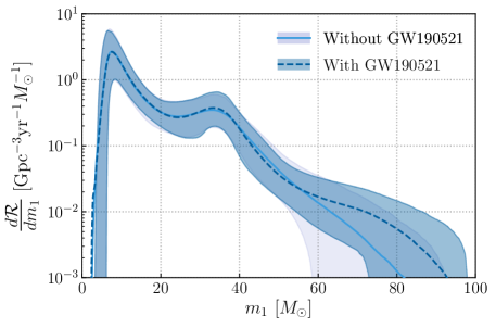
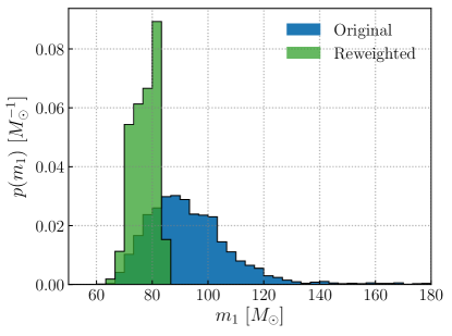
C.3 On GW190814
On the other hand, we see clear indication that \IfEqCaseGW190814AGW190413AGW190413_052954GW190719AGW190719_215514GW190620AGW190620_030421GW190514AGW190514_065416GW190731AGW190731_140936GW190503AGW190503_185404GW190602AGW190602_175927GW190929AGW190929_012149GW190517AGW190517_055101GW190915AGW190915_235702GW190425AGW190425GW190512AGW190512_180714GW190630AGW190630_185205GW190521AGW190521GW190413BGW190413_134308GW190924AGW190924_021846GW190930AGW190930_133541GW190706AGW190706_222641GW190408AGW190408_181802GW190909AGW190909_114149GW190728AGW190728_064510GW190426AGW190426_152155GW190412AGW190412GW190720AGW190720_000836GW190521BGW190521_074359GW190910AGW190910_112807GW190803AGW190803_022701GW190519AGW190519_153544GW190708AGW190708_232457GW190527AGW190527_092055GW190513AGW190513_205428GW190424AGW190424_180648GW190727AGW190727_060333GW190814AGW190814GW190707AGW190707_093326GW190828AGW190828_063405GW190828BGW190828_065509GW190701AGW190701_203306GW190421AGW190421_213856 is an outlier with respect to the BBH population within the framework of the Power Law + Peak and Broken Power Law mass models, as discussed in Section 5.1. As an additional posterior predictive check, following the analysis described in Fishbach et al. (2020b) and Abbott et al. (2020a), we use the posterior predictive distribution, inferred without \IfEqCaseGW190814AGW190413AGW190413_052954GW190719AGW190719_215514GW190620AGW190620_030421GW190514AGW190514_065416GW190731AGW190731_140936GW190503AGW190503_185404GW190602AGW190602_175927GW190929AGW190929_012149GW190517AGW190517_055101GW190915AGW190915_235702GW190425AGW190425GW190512AGW190512_180714GW190630AGW190630_185205GW190521AGW190521GW190413BGW190413_134308GW190924AGW190924_021846GW190930AGW190930_133541GW190706AGW190706_222641GW190408AGW190408_181802GW190909AGW190909_114149GW190728AGW190728_064510GW190426AGW190426_152155GW190412AGW190412GW190720AGW190720_000836GW190521BGW190521_074359GW190910AGW190910_112807GW190803AGW190803_022701GW190519AGW190519_153544GW190708AGW190708_232457GW190527AGW190527_092055GW190513AGW190513_205428GW190424AGW190424_180648GW190727AGW190727_060333GW190814AGW190814GW190707AGW190707_093326GW190828AGW190828_063405GW190828BGW190828_065509GW190701AGW190701_203306GW190421AGW190421_213856, to construct a distribution for the minimum detected in a sample of 45 events. When using both the Power Law + Peak and Broken Power Law models, we find that the observation of a system with a secondary mass equal to or smaller than the that of \IfEqCaseGW190814AGW190413AGW190413_052954GW190719AGW190719_215514GW190620AGW190620_030421GW190514AGW190514_065416GW190731AGW190731_140936GW190503AGW190503_185404GW190602AGW190602_175927GW190929AGW190929_012149GW190517AGW190517_055101GW190915AGW190915_235702GW190425AGW190425GW190512AGW190512_180714GW190630AGW190630_185205GW190521AGW190521GW190413BGW190413_134308GW190924AGW190924_021846GW190930AGW190930_133541GW190706AGW190706_222641GW190408AGW190408_181802GW190909AGW190909_114149GW190728AGW190728_064510GW190426AGW190426_152155GW190412AGW190412GW190720AGW190720_000836GW190521BGW190521_074359GW190910AGW190910_112807GW190803AGW190803_022701GW190519AGW190519_153544GW190708AGW190708_232457GW190527AGW190527_092055GW190513AGW190513_205428GW190424AGW190424_180648GW190727AGW190727_060333GW190814AGW190814GW190707AGW190707_093326GW190828AGW190828_063405GW190828BGW190828_065509GW190701AGW190701_203306GW190421AGW190421_213856 () is highly improbable, with probability for both Power Law + Peak and Broken Power Law; see Fig. 22b for the distribution of the minimum observed secondary mass in a sample of 45 events predicted by the Power Law + Peak model. The distribution for Broken Power Law is qualitatively similar. The mass ratio of \IfEqCaseGW190814AGW190413AGW190413_052954GW190719AGW190719_215514GW190620AGW190620_030421GW190514AGW190514_065416GW190731AGW190731_140936GW190503AGW190503_185404GW190602AGW190602_175927GW190929AGW190929_012149GW190517AGW190517_055101GW190915AGW190915_235702GW190425AGW190425GW190512AGW190512_180714GW190630AGW190630_185205GW190521AGW190521GW190413BGW190413_134308GW190924AGW190924_021846GW190930AGW190930_133541GW190706AGW190706_222641GW190408AGW190408_181802GW190909AGW190909_114149GW190728AGW190728_064510GW190426AGW190426_152155GW190412AGW190412GW190720AGW190720_000836GW190521BGW190521_074359GW190910AGW190910_112807GW190803AGW190803_022701GW190519AGW190519_153544GW190708AGW190708_232457GW190527AGW190527_092055GW190513AGW190513_205428GW190424AGW190424_180648GW190727AGW190727_060333GW190814AGW190814GW190707AGW190707_093326GW190828AGW190828_063405GW190828BGW190828_065509GW190701AGW190701_203306GW190421AGW190421_213856 is also somewhat unusual according to this posterior predictive check; see Fig. 22a. Observing an event with the mass ratio of \IfEqCaseGW190814AGW190413AGW190413_052954GW190719AGW190719_215514GW190620AGW190620_030421GW190514AGW190514_065416GW190731AGW190731_140936GW190503AGW190503_185404GW190602AGW190602_175927GW190929AGW190929_012149GW190517AGW190517_055101GW190915AGW190915_235702GW190425AGW190425GW190512AGW190512_180714GW190630AGW190630_185205GW190521AGW190521GW190413BGW190413_134308GW190924AGW190924_021846GW190930AGW190930_133541GW190706AGW190706_222641GW190408AGW190408_181802GW190909AGW190909_114149GW190728AGW190728_064510GW190426AGW190426_152155GW190412AGW190412GW190720AGW190720_000836GW190521BGW190521_074359GW190910AGW190910_112807GW190803AGW190803_022701GW190519AGW190519_153544GW190708AGW190708_232457GW190527AGW190527_092055GW190513AGW190513_205428GW190424AGW190424_180648GW190727AGW190727_060333GW190814AGW190814GW190707AGW190707_093326GW190828AGW190828_063405GW190828BGW190828_065509GW190701AGW190701_203306GW190421AGW190421_213856 or smaller, based on the fit to the other 44 BBH events, has probability in both the Power Law + Peak and Broken Power Law models. These posterior predictive checks suggest that \IfEqCaseGW190814AGW190413AGW190413_052954GW190719AGW190719_215514GW190620AGW190620_030421GW190514AGW190514_065416GW190731AGW190731_140936GW190503AGW190503_185404GW190602AGW190602_175927GW190929AGW190929_012149GW190517AGW190517_055101GW190915AGW190915_235702GW190425AGW190425GW190512AGW190512_180714GW190630AGW190630_185205GW190521AGW190521GW190413BGW190413_134308GW190924AGW190924_021846GW190930AGW190930_133541GW190706AGW190706_222641GW190408AGW190408_181802GW190909AGW190909_114149GW190728AGW190728_064510GW190426AGW190426_152155GW190412AGW190412GW190720AGW190720_000836GW190521BGW190521_074359GW190910AGW190910_112807GW190803AGW190803_022701GW190519AGW190519_153544GW190708AGW190708_232457GW190527AGW190527_092055GW190513AGW190513_205428GW190424AGW190424_180648GW190727AGW190727_060333GW190814AGW190814GW190707AGW190707_093326GW190828AGW190828_063405GW190828BGW190828_065509GW190701AGW190701_203306GW190421AGW190421_213856 is not a typical BBH, and support the conclusion that there may be a dearth of systems between and . Future observations will reveal the precise shape of the mass distribution at low masses and extreme mass ratios, and better determine the nature of \IfEqCaseGW190814AGW190413AGW190413_052954GW190719AGW190719_215514GW190620AGW190620_030421GW190514AGW190514_065416GW190731AGW190731_140936GW190503AGW190503_185404GW190602AGW190602_175927GW190929AGW190929_012149GW190517AGW190517_055101GW190915AGW190915_235702GW190425AGW190425GW190512AGW190512_180714GW190630AGW190630_185205GW190521AGW190521GW190413BGW190413_134308GW190924AGW190924_021846GW190930AGW190930_133541GW190706AGW190706_222641GW190408AGW190408_181802GW190909AGW190909_114149GW190728AGW190728_064510GW190426AGW190426_152155GW190412AGW190412GW190720AGW190720_000836GW190521BGW190521_074359GW190910AGW190910_112807GW190803AGW190803_022701GW190519AGW190519_153544GW190708AGW190708_232457GW190527AGW190527_092055GW190513AGW190513_205428GW190424AGW190424_180648GW190727AGW190727_060333GW190814AGW190814GW190707AGW190707_093326GW190828AGW190828_063405GW190828BGW190828_065509GW190701AGW190701_203306GW190421AGW190421_213856.
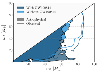
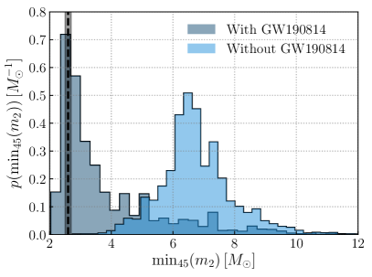
C.4 Mass and distance checks with a burst analysis
The cWB analysis resulted in the detection of 22 BBH events in GWTC-2. We investigate whether the set of cWB observations is consistent with the model predictions. In particular, we examine whether \IfEqCaseGW190521AGW190413AGW190413_052954GW190719AGW190719_215514GW190620AGW190620_030421GW190514AGW190514_065416GW190731AGW190731_140936GW190503AGW190503_185404GW190602AGW190602_175927GW190929AGW190929_012149GW190517AGW190517_055101GW190915AGW190915_235702GW190425AGW190425GW190512AGW190512_180714GW190630AGW190630_185205GW190521AGW190521GW190413BGW190413_134308GW190924AGW190924_021846GW190930AGW190930_133541GW190706AGW190706_222641GW190408AGW190408_181802GW190909AGW190909_114149GW190728AGW190728_064510GW190426AGW190426_152155GW190412AGW190412GW190720AGW190720_000836GW190521BGW190521_074359GW190910AGW190910_112807GW190803AGW190803_022701GW190519AGW190519_153544GW190708AGW190708_232457GW190527AGW190527_092055GW190513AGW190513_205428GW190424AGW190424_180648GW190727AGW190727_060333GW190814AGW190814GW190707AGW190707_093326GW190828AGW190828_063405GW190828BGW190828_065509GW190701AGW190701_203306GW190421AGW190421_213856 is an outlier in the context of our mass and redshift models. Following Klimenko et al. (2016), we calculate the expected distribution of the central frequency and coherent signal-to-noise ratio for two different population models: Power Law + Peak and Broken Power Law, using the Non-Evolving redshift model. We then compare the empirical distribution of , as recovered by the cWB pipeline to the distribution predicted by the population model. We quantify the comparison by calculating a -value for each event , which measures how unusual its observed is, given the distribution of predicted . The central frequency is a proxy for the redshifted mass while the signal-to-noise ratio is a proxy for the distance.
To compute the predicted distribution of , we inject simulated waveforms drawn from the Power Law + Peak and Broken Power Law distributions into the O1, O2 and O3a data and compile injections recovered by cWB with a . The central frequencies and coherent signal-to-noise ratios of the recovered injections generated according to Power Law + Peak are plotted in Fig. 23. The results for Broken Power Law are similar. The locations of the 22 detections on this plane are visually consistent with the model predictions, indicating that the model is a reasonably good fit to the data. The event with the lowest -value (least consistent with predictions) is \IfEqCaseGW190521AGW190413AGW190413_052954GW190719AGW190719_215514GW190620AGW190620_030421GW190514AGW190514_065416GW190731AGW190731_140936GW190503AGW190503_185404GW190602AGW190602_175927GW190929AGW190929_012149GW190517AGW190517_055101GW190915AGW190915_235702GW190425AGW190425GW190512AGW190512_180714GW190630AGW190630_185205GW190521AGW190521GW190413BGW190413_134308GW190924AGW190924_021846GW190930AGW190930_133541GW190706AGW190706_222641GW190408AGW190408_181802GW190909AGW190909_114149GW190728AGW190728_064510GW190426AGW190426_152155GW190412AGW190412GW190720AGW190720_000836GW190521BGW190521_074359GW190910AGW190910_112807GW190803AGW190803_022701GW190519AGW190519_153544GW190708AGW190708_232457GW190527AGW190527_092055GW190513AGW190513_205428GW190424AGW190424_180648GW190727AGW190727_060333GW190814AGW190814GW190707AGW190707_093326GW190828AGW190828_063405GW190828BGW190828_065509GW190701AGW190701_203306GW190421AGW190421_213856, with -values of 0.053 and 0.077 for the Broken Power Law model and the Power Law + Peak model respectively. These -values indicate that \IfEqCaseGW190521AGW190413AGW190413_052954GW190719AGW190719_215514GW190620AGW190620_030421GW190514AGW190514_065416GW190731AGW190731_140936GW190503AGW190503_185404GW190602AGW190602_175927GW190929AGW190929_012149GW190517AGW190517_055101GW190915AGW190915_235702GW190425AGW190425GW190512AGW190512_180714GW190630AGW190630_185205GW190521AGW190521GW190413BGW190413_134308GW190924AGW190924_021846GW190930AGW190930_133541GW190706AGW190706_222641GW190408AGW190408_181802GW190909AGW190909_114149GW190728AGW190728_064510GW190426AGW190426_152155GW190412AGW190412GW190720AGW190720_000836GW190521BGW190521_074359GW190910AGW190910_112807GW190803AGW190803_022701GW190519AGW190519_153544GW190708AGW190708_232457GW190527AGW190527_092055GW190513AGW190513_205428GW190424AGW190424_180648GW190727AGW190727_060333GW190814AGW190814GW190707AGW190707_093326GW190828AGW190828_063405GW190828BGW190828_065509GW190701AGW190701_203306GW190421AGW190421_213856 is a moderately unusual detection, but it is consistent with the population models.
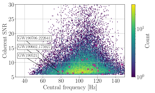
Appendix D Details of spin population models
D.1 Default spin model
This model was introduced in Abbott et al. (2019a). Following Wysocki et al. (2019a), the dimensionless spin magnitude distribution is taken to be a Beta distribution,
| (D1) |
where and are the standard shape parameters that determine the distribution’s mean and variance. The Beta distribution is convenient because it is bounded on (0,1). The distributions for and are assumed to be the same. Following Talbot & Thrane (2017), we define as the cosine of the tilt angle between component spin and a binary’s orbital angular momentum, and assume that is distributed as a mixture of two populations:
| (D2) |
Here, is an isotropic distribution, while is a truncated Gaussian, peaking at (perfect alignment) with width . The mixing parameter controls the relative fraction of mergers drawn from the isotropic distribution and Gaussian subpopulations. The isotropic subpopulation is intended to accommodate dynamically assembled binaries, while is a model for field mergers. The hyper-parameters for this model and their priors are summarized in Table 9. Additional constraints to the priors on and are applied by setting , .
In Fig. 24 we provide a corner plot for the Default spin model. This model prefers modest spin magnitudes. It favors the hypothesis that binaries are preferentially aligned ( and ), albeit with potentially large misalignment angles (). The case of perfect alignment, which would correspond to and , is disfavored, lying outside the 99% credible bound on and . Within the main text, Fig. 10 shows the implied distributions of component spin magnitudes and tilt angles. The implied distributions of the effective precession spin parameter () and the effective inspiral spin parameter () are shown in Figs. 9 and 11, respectively; these distributions are in good agreement with the results obtained using the Gaussian model described below. In particular, both models predict the existence of systems with anti-aligned spins (negative ), and in-plane spin components (non-zero ).
| Parameter | Description | Prior | |
|---|---|---|---|
| Mean of the Beta distribution of spin magnitudes. | U(0,1) | ||
| Variance of the Beta distribution of spin magnitudes. | U(0,0.25) | ||
| Mixing fraction of mergers from truncated Gaussian distribution. | U(0,1) | ||
| Width of truncated Gaussian, determining typical spin misalignment. | U(0.01,4) |
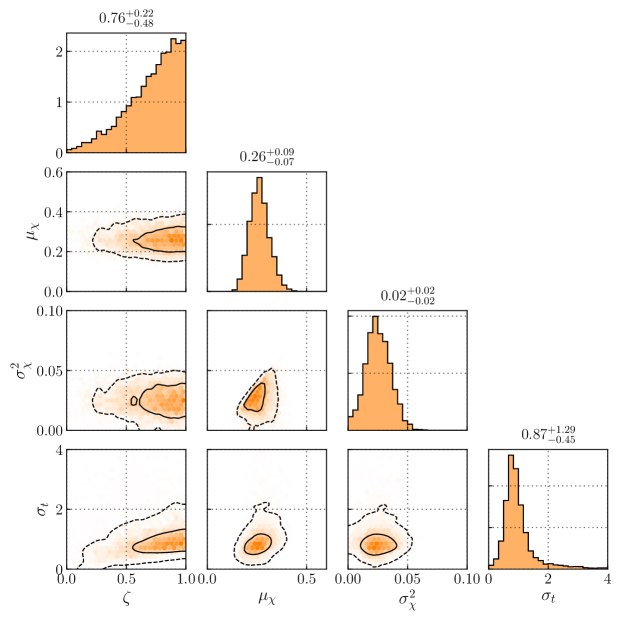
D.2 Gaussian spin model
The Gaussian spin model offers an alternative description of BBH spins. It is convenient to measure the distribution of the effective inspiral spin parameter () and the effective precession spin parameter (), which are better constrained than individual component spin magnitudes or tilts. We parameterize the distributions of and , using a bivariate Gaussian:
| (D3) |
The distribution has a mean and a covariance matrix
| (D4) |
The population parameters appearing in Eqs. (D3) and (D4) and their associated priors are summarized in Table 10. We truncate and normalize Eq. (D3) based on the allowed regions of the effective inspiral spin parameter: and . The results from the Gaussian model are obtained assuming a Truncated mass model with , , , and , consistent with the median values obtained when fitting the Truncated model to GWTC-2. We additionally assume a comoving merger rate density that grows as . Although the Truncated model is disfavored relative to the more complex mass models discussed above, it is sufficient for purposes of constructing an informed mass ratio distribution, the primary confounding factor in efforts to measure and (Ng et al., 2018a).
| Parameter | Description | Prior | |
|---|---|---|---|
| Mean of the distribution. | U(, ) | ||
| Standard deviation of the distribution. | U(0.01,1) | ||
| Mean of the distribution. | U(, ) | ||
| Standard deviation of the distribution. | U(, ) | ||
| Degree of correlation between and . | U(, ) |
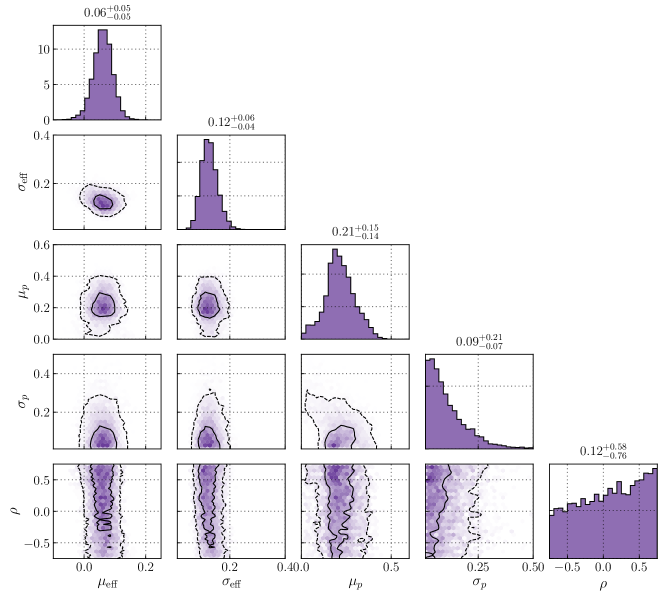
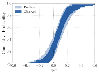
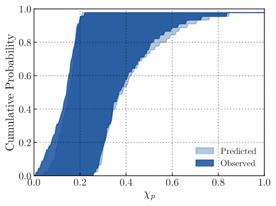
We find no correlation between the parameters of the and distributions, nor do we obtain any information regarding the degree of correlation between the effective inspiral spin parameter and the effective precession spin parameter. As discussed in Sec. 5.2, analysis with the Gaussian spin model
With the Gaussian model, we also find evidence that at least some BHs have anti-aligned spins, with , such that . To further evaluate the robustness of our Gaussian model fits, in Fig. 26 we show posterior predictive comparisons between predicted and empirical catalogs of and measurements. The light blue bands mark 90% credible bounds on the predicted cumulative distribution of observed effective inspiral spin parameter values, given our posterior on the Gaussian model parameters. The dark shaded regions, meanwhile, show 90% credible bounds on the true distribution observed within GWTC-2, achieved by reweighting single event and by repeated random draws from the Gaussian hyper-posterior.
There are several sources of possible bias that might influence our Gaussian model conclusions. One possible source of bias is the mass model presumed for the Gaussian spin analysis. As noted above, measurements of a binary’s and mass ratio are generally anti-correlated (Ng et al., 2018a). Therefore, our particular choice of could conceivably affect conclusions regarding the distribution. We have directly verified that the results in Fig. 27 remain robust under different fiducial choices of between and .
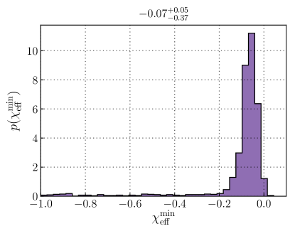
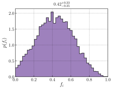
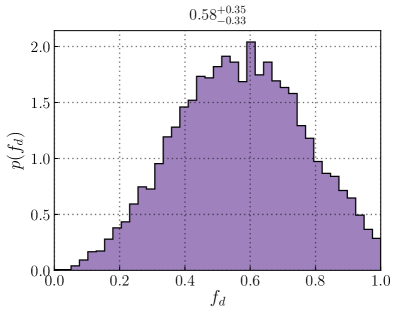
Another source of bias may be the Gaussian functional form we impose on the and distributions, enforcing a unimodal distribution with smooth tails. As discussed in Sec. 5.2, though, the Default spin model yields near-identical and distributions, despite its different parametrization and different physical assumptions. As an additional check, we repeat the Gaussian spin analysis on our data, truncating the distribution not on , but on , where is inferred from the data. Figure 27 shows the marginal posterior for . We find that is constrained to be negative at credibility, confirming that support for negative effective inspiral spin parameter is a feature of the data and not simply an artifact of the Gaussian model.
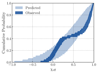
D.3 Multi Spin model
This model is an extension of the Truncated mass model with an additional Gaussian component. It is similar to the Power Law + Peak model, but there are several differences. First, the high-mass subpopulation in Multi Spin is described by a Gaussian in both and (up to the truncation) while Power Law + Peak only models as a Gaussian, and assumes that all BBH systems are described by a power-law distribution in mass ratio . Most importantly, as its name suggests, Multi Spin allows each subpopulation to have its own independent spin distribution, each of which follows the Default model, with . This allows us to probe whether the spin distribution varies with mass. The parameters for Multi Spin are summarized in Table 11.
| Parameter | Description | Prior | |
|---|---|---|---|
| Local merger rate for the low-mass power-law subpopulation. | U() | ||
| Local merger rate for the high-mass Gaussian subpopulation. | U() | ||
| Power-law slope of the primary mass distribution for the low-mass subpopulation. | U() | ||
| Power-law slope of the mass ratio distribution for the low-mass subpopulation | U() | ||
| Minimum mass of the primary mass distribution for the low-mass subpopulation. | U() | ||
| Maximum mass of the primary mass distribution for the low-mass subpopulation. | U() | ||
| Centroid of the primary mass distribution for the high-mass subpopulation | U() | ||
| Width of the primary mass distribution for the high-mass subpopulation | U() | ||
| Centroid of the secondary mass distribution for the high-mass subpopulation | U() | ||
| Width of the secondary mass distribution for the high-mass subpopulation | U() | ||
| Mean of the beta distribution of primary spin magnitudes for the low-mass subpopulation. | U() | ||
| Variance of the beta distribution of primary spin magnitudes for the low-mass subpopulation. | U() | ||
| Width of the truncated Gaussian distribution of (primary spin tilt angle) for the low-mass subpopulation. | U() | ||
| Mean of the beta distribution of secondary spin magnitudes for the low-mass subpopulation. | U() | ||
| Variance of the beta distribution of secondary spin magnitudes for the low-mass subpopulation. | U() | ||
| Width of the truncated Gaussian distribution of (secondary spin tilt angle) for the low-mass subpopulation. | U() | ||
| Mean of the beta distribution of primary spin magnitudes for the high-mass subpopulation. | U() | ||
| Variance of the beta distribution of primary spin magnitudes for the high-mass subpopulation. | U() | ||
| Width of the truncated Gaussian distribution of (primary spin tilt angle) for the high-mass subpopulation. | U() | ||
| Mean of the beta distribution of secondary spin magnitudes for the high-mass subpopulation. | U() | ||
| Variance of the beta distribution of secondary spin magnitudes for the high-mass subpopulation. | U() | ||
| Width of the truncated Gaussian distribution of (secondary spin tilt angle) for the high-mass subpopulation. | U() |
Appendix E Redshift Evolution Models
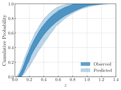
The power-law redshift evolution model parameterizes the merger rate density as
| (E1) |
where denotes the merger rate density at . This implies that the redshift distribution is
| (E2) |
where is the differential comoving volume, and is related to by
| (E3) |
We take in the analysis, as this is a conservative upper bound on the redshift at which we could detect BBH systems during O3a within the mass range considered here. When fitting this model, we employ a uniform prior on centered at . The value corresponds to no evolution; i.e., a merger rate that is uniform-in-comoving volume and source-frame time. We take a sufficiently wide prior so that the likelihood is entirely within the prior range, .
Appendix F Gravitational-wave lensing
It has been suggested that gravitational-wave lensing could bias the estimate of binary masses (Dai et al., 2017; Ng et al., 2018b; Li et al., 2018; Oguri, 2018; Hannuksela et al., 2019), which could lead to a biased population inference. However, based on the predictions on the number of expected gravitational-wave sources and the distribution of galaxy lenses in the Universe, Li et al. (2018); Oguri (2018) predict that only around one in a thousand observed events are lensed, although this estimate can vary depending on the redshift evolution of the merger-rate density. The lensing rate is expected to be similarly rare for galaxy clusters (Smith et al., 2018). As the expected lensing rate is low compared to the number of events in GWTC-2, we assume that all events in our sample are unlensed.