Self-learning Monte-Carlo for non-abelian gauge theory with dynamical fermions

Abstract

In this paper, we develop the self-learning Monte-Carlo (SLMC) algorithm for non-abelian gauge theory with dynamical fermions in four dimensions to resolve the autocorrelation problem in lattice QCD. We perform simulations with the dynamical staggered fermions and plaquette gauge action by both in HMC and SLMC for zero and finite temperature to examine the validity of SLMC. We confirm that SLMC can reduce autocorrelation time in non-abelian gauge theory and reproduces results from HMC. For finite temperature runs, we confirm that SLMC reproduces correct results with HMC, including higher-order moments of the Polyakov loop and the chiral condensate. Besides, our finite temperature calculations indicate that four flavor QC₂D with $\hat{m}=0.5$ is likely in the crossover regime in the Colombia plot.

I Introduction

For more than 40 years, numerical calculations of lattice QCD have been an established technique to calculate QCD observables including non-perturbative effects [1]. Lattice QCD is based on the Markov chain Monte-Carlo (MCMC) algorithms with the detailed balance condition, which guarantees the MCMC process’s convergence, and it is crucial for dealing with the dimensionality of the path integral for lattice QCD. From a practical point of view, guaranteeing the convergence is inevitable because it allows for uses of the computational result in precise phenomenology. (See [2, 3] and references therein, for example).

A MCMC algorithm for lattice QCD is required following three conditions. The first condition is, convergence of the Markov chain update. Typically, one requires the detailed balance condition because it is a sufficient condition for the convergence. The second condition is applicability for a non-abelian gauge system with dynamical fermions because QCD consists of gluons and quarks, and we must guarantee the gauge invariance. The third condition is no-bias in calculations. For example, the hybrid algorithm or R algorithm can deal with dynamical fermions, but it has a bias [4], and it is not favored. Another example is the molecular dynamics, which can generate configurations for lattice QCD by itself, but its ergodicity is not guaranteed.

De facto standard algorithms for gauge theories with dynamical fermions are the hybrid Monte-Carlo (HMC) [5] and its variant rational hybrid Monte-Carlo (RHMC) [6] because they satisfy the three conditions above. The basic idea of (R)HMC is based on the Metropolis algorithm with fictitious hamiltonian dynamics, including Gaussian momentum, along with a fictitious time. Generally speaking, a Metropolis algorithm enjoys high efficiency if the theory’s energy function does not change so much during the update process. (R)HMC uses the molecular dynamics with a reversible symplectic integrator, and it preserves the energy function mostly. The Gaussian momentum guarantees ergodicity of the algorithm. In addition to this update process allows us to include fermions through the pseudofermion trick. Despite these advantages, (R)HMC suffers from unavoidable critical slowing down problem with several parameter regimes [7, 8, 9], and thus to resolve the problem, a new algorithm is demanded.

On the other hand, recent progress of machine (ML) learning drives application it to lattice field theory [10, 11, 12, 13, 14, 15, 16, 17, 18, 19, 20, 21, 22, 23, 24, 25, 26, 27, 28, 29, 30]. There are three typical usages of machine learning in this context. The first is making a detector of phase boundaries [11, 31, 12]. The second is calculation for observable to reduce numerical cost [13, 14, 15, 16]. The third is configuration generation for field theory [17, 18, 19, 20, 21, 22]. These applications are inspired by similarities between configuration generation and image generation but except for flow-based algorithm [20, 21, 22], they do not enjoy the convergence theorem. This means that one has to compare observables one by one with observables generated by a “legal algorithm” like HMC.

Self-learning Monte-Carlo(SLMC) is a machine-learning based configuration generation algorithm [32, 33, 34, 35, 36, 37, 38]. Originally it has been developed for a classical spin model [32] but it works widely among quantum model in condensed matter physics and quantum chemistry [33, 36]. SLMC employs updates using a tunable action with an efficient update algorithm and the Metropolis – Hastings test, and then, it becomes an exact algorithm. One of the advantages of SLMC is interpretability; we can use our insight of the original theory to construct the tunable action. Besides, one can also use neural networks to evaluate the tunable action in the algorithm [34, 36] by giving up interpretability in order to achieve better acceptance. We develop SLMC for non-abelian gauge field with dynamical fermions.

From 90s, systems with dynamical fermions using hopping parameter expanded action have been investigated [39, 40, 41, 42, 43, 44]. They used truncated determinant to perform simulations for the Schwinger model and zero temperature QCD. Here we clarify the difference between the present work and these studies. First, we perform an extensive study for volume dependence and action dependence, and we find that the Polyakov loop in the effective action improves acceptance. Second, we (re-)formulated the algorithm in the context of ML application. It clarifies the meanings and possible extension of the algorithm. Thirds, we confirm our algorithm reduce autocorrelation for a finite temperature system. As an similar idea, the multi-boson algorithm [45, 46] is known. It uses the Metropolis algorithm with polynomially expanded fermion action. But we do not use pseudofermion field to update the gauge field in the present work. We leave that idea for future study.

In this work, we perform simulations with two-color QCD with dynamical fermions in four dimensions (QC₂D) using HMC and SLMC. Besides, we apply our algorithm to investigate QC₂D with 4 flavors phase diagram associated the Polyakov loop in heavy mass regime at finite temperature. In that regime, HMC is suffered from long autocorrelation problem of the Polyakov loop. We find that, both in zero and finite temperature, SLMC has smaller autocorrelation time than HMC and gives consistent results with correct cumulants.

This paper is organized as follows. In section 2, we review self-learning Monte-Carlo from Metropolis – Hasting algorithm. In section 3, we explain our target system and our effective action in our calculations. In section 4, we introduce our results at zero temperature runs. In section 5, we show results for an application of SLMC to a finite temperature system. In section 6, we summarize our results.

II Self-learning Monte-Carlo

Here we briefly derive the self-learning Monte-Carlo algorithm from the Metropolis–Hasting algorithm for gauge theories to be self-contained.

II.1 Metropolis-Hasting algorithm

To generate configurations with a Markov-chain, we need to design a conditioned probability $P(B|A)$, where $A$ is a seed configuration and $B$ is a generated configuration. The Metropolis–Hasting algorithm is based on the detailed balance condition,

$$W_{A}P(B|A)={W_{B}}P(A|B),$$ (1)

where $A$ and $B$ are a label for configurations and $W_{A}$ is the Boltzmann weight proportional to $\text{e}^{-S[U_{A}]}$ for a configuration $U_{A}$ with action $S\in\mathbb{R}$. This guarantees configurations which are generated by the algorithm are distributed with the desired distribution associated with $W\propto\text{e}^{-S}$. The Metropolis–Hasting algorithm is defined by following update rule,

$$P_{\text{MH}}(B|A)\equiv\min\left(1,\frac{W_{B}T(A|B)}{W_{A}T(B|A)}\right)T(B|A),$$ (2)

where $T(B|A)$ represents a proposing process, which makes a candidate configuration $B$ from $A$ and $\min(\cdots)$ denotes the Metropolis test. Note that the process $T(B|A)$ does not have to be reversible in spite of the molecular dynamics in HMC has to be reversible. If one requires the reversibility to $T(B|A)$, it is reduced to the simplest Metropolis algorithm. The detailed balance condition can be reproduced from the update algorithm:

$$P_{\text{MH}}(B|A) =\frac{W_{B}T(A|B)}{W_{A}T(B|A)}\min\left(1,\frac{W_{A}T(B|A)}{W_{B}T(A|B)}\right)T(B|A),$$ (3)

$$=\frac{W_{B}}{W_{A}}P_{\text{MH}}(A|B).$$ (4)

In the first line we used an identity $\min(1,c)=c\min(1,1/c)$ and $c$ is a non-negative real number. In this manner, we can reproduce the detailed balance condition from the Metropolis-Hasting update rule.

II.2 Self-learning Monte-Carlo

Self-learning Monte Carlo (SLMC) is one of the Metropolis-Hasting algorithms. It is obtained by regarding $T(B|A)=P^{\text{eff}}_{\theta}(B|A)$, which is an update algorithm associated with an effective action with a set of parameters $\theta$ like couplings in the effective model. The parameter set $\theta$ is determined by a machine learning estimator, and we use the linear regression in this work. In the framework of SLMC, the effective action has to have an efficient update algorithm with the detailed balance for the effective action,

$$\frac{W_{A}^{\text{eff,$\theta$}}}{W_{B}^{\text{eff,$\theta$}}}=\frac{P^{\text{eff}}_{\theta}(A|B)}{P^{\text{eff}}_{\theta}(B|A)}.$$ (5)

Let us regard $T(B|A)$ as $P^{\text{eff}}_{\theta}(B|A)$ in the Metropolis Hasting algorithm,

$$P_{\text{SLMC}}(B|A) \equiv\min\left(1,\frac{W_{B}P^{\text{eff}}_{\theta}(A|B)}{W_{A}P^{\text{eff}}_{\theta}(B|A)}\right)P^{\text{eff}}_{\theta}(B|A),$$ (6)

and this is the update rule for the self-learning Monte-Carlo. The detailed balance can be derived from this update,

$$P_{\text{SLMC}}(B|A) =\frac{W_{B}P^{\text{eff}}_{\theta}(A|B)}{W_{A}P^{\text{eff}}_{\theta}(B|A)}\min\left(1,\frac{W_{A}P^{\text{eff}}_{\theta}(B|A)}{W_{B}P^{\text{eff}}_{\theta}(A|B)}\right)P^{\text{eff}}_{\theta}(B|A),$$ (7)

$$=\frac{W_{B}}{W_{A}}\min\left(1,\frac{W_{A}P^{\text{eff}}_{\theta}(B|A)}{W_{B}P^{\text{eff}}_{\theta}(A|B)}\right)P^{\text{eff}}_{\theta}(A|B),$$ (8)

$$=\frac{W_{B}}{W_{A}}P_{\text{SLMC}}(A|B).$$ (9)

The self-learning update satisfies the detailed balance and it will converge. The modified Metropolis test can be evaluated with the effective action because of (5) and,

$$\min\left(1,\frac{W_{B}P^{\text{eff}}_{\theta}(A|B)}{W_{A}P^{\text{eff}}_{\theta}(B|A)}\right) =\min\left(1,\frac{W_{B}}{W_{A}}\frac{W_{A}^{\text{eff,$\theta$}}}{W_{B}^{\text{eff,$\theta$}}}\right)=\min\left(1,\frac{W_{B}/W_{B}^{\text{eff,$\theta$}}}{W_{A}/W_{A}^{\text{eff,$\theta$}}}\right).$$ (10)

Here we do not have to assume reversibility for $T=P^{\text{eff}}_{\theta}$ again but it requires the detailed balance for the effective action instead. Note that, if one uses an effective action which differs from the target system’s one, the acceptance rate could be low but even such case the expectation values still converge into the exact values with long autocorrelation (i.e., large statistical error) because this is an exact algorithm.

III Numerical setup

In this section, we introduce our numerical setup. Though out this paper, we show every quantity in lattice unit. We perform simulations with $SU(2)$ plaquette action with 4 tastes standard staggered fermions for implementational simplicity. Our target system is described by the action $S[U,\overline{\chi},\chi]$,

$$S[U,\overline{\chi},\chi] =S_{g}[U]+\sum_{n}(\overline{\chi}M[U]\chi)_{n},$$ (11)

where $S_{g}[U]$ is the Wilson plaquette action,

$$S_{g}[U] =\beta\sum_{n}\sum_{\mu=1}^{4}\sum_{\nu>\mu}\left(1-\frac{1}{2}\mathrm{tr}\,U_{\mu\nu}(n)\right),$$ (12)

$$U_{\mu\nu}(n) =U_{\mu}(n)U_{\nu}(n+\hat{\mu})U_{\mu}^{\dagger}(n+\hat{\nu})U_{\nu}^{\dagger}(n),$$ (13)

and $M[U]$ is a massive staggered Dirac operator,

$$M[U]\chi =\frac{1}{2}\sum_{\mu=1}^{4}\eta_{\mu}(n)\left[U_{\mu}(n)\chi(n+\hat{\mu})-U_{\mu}^{\dagger}(n-\hat{\mu})\chi(n-\hat{\mu})\right]+\hat{m}\chi(n),$$ (14)

and $\eta_{\mu}(n)$ is the staggered factor. $U_{\mu}(n)$ is a link variable for $SU(2)$ gauge field, and $\chi(n)$ is a single component spinor field. $\hat{m}$ is a quark mass in the lattice unit.

All numerical calculations for HMC and SLMC are performed by Julia [48] and the code is developed by ourselves. In addition, we implement automatic generation of heatbath code which generates staples from given loop operators [49]. This enables us to investigate effective action with various types of extended loops. However, in present work, we employ the effective action (18) for simplicity and study with complicated loops leave it as a future work.

III.1 SLMC setup

SLMC update probability for the lattice gauge theory is written as,

$$P_{\text{SLMC}}(U^{\prime}|U)=\min\left(1,\frac{e^{-(S[U^{\prime}]-S^{\theta}_{\text{eff}}[U^{\prime}])}}{e^{-(S[U]-S^{\theta}_{\text{eff}}[U])}}\right)P^{\theta}_{\text{eff}}(U^{\prime}|U),$$ (15)

where our target action in bosonic language is given by,

$$S[U]=S_{g}[U]+S_{f}[U],$$ (16)

where $S_{g}[U]$ is the plaquette gauge action and,

$$S_{f}[U]=-\log\det M^{\dagger}M,$$ (17)

and $S^{\theta}_{\text{eff}}[U]$ is an effective action with tunable parameters, which is only consisted by loop operators e.g., plaquette and rectangular and so on. We use exact diagonalization to evaluate the Dirac operator in this paper for simplicity and this can be improved by using stochastic estimator in the reweighting technique [50, 51]. We call this algorithm as self-learning Monte-Carlo (SLMC) hereafter.

In practice, we employ heavy mass expanded fermion action with truncation [52] for updates in SLMC. Our effective action is consisted by the plaquette, rectangular loops and the Polyakov loop for $\mu=1,2,3,4$ directions. Let us denote $\vec{n}=(n_{1},n_{2},n_{3})$ is spatial coordinate and $n_{4}$ is the temporal direction and let lattice size be $N_{1},N_{2},N_{3}$ and $N_{4}$ for spatial and temporal extent, respectively. The effective action is,

$$S^{\theta}_{\text{eff}}[U] =\sum_{n}\left[\beta_{\text{plaq}}\sum_{\mu=1}^{4}\sum_{\nu>\mu}\left(1-\frac{1}{2}\mathrm{tr}\,U_{\mu\nu}(n)\right)+\beta_{\text{rect}}\sum_{\mu=1}^{4}\sum_{\nu\neq\mu}\left(1-\frac{1}{2}\mathrm{tr}\,R_{\mu\nu}(n)\right)\right]$$

$$\;\;\;\;\;\;+\beta^{\mu=1}_{\text{Pol}}\sum_{n_{2},n_{3},n_{4}}\mathrm{tr}\,\big{[}\prod_{n_{1}=0}^{N_{1}-1}U_{1}(\vec{n},n_{4})\big{]}+\beta^{\mu=2}_{\text{Pol}}\sum_{n_{1},n_{3},n_{4}}\mathrm{tr}\,\big{[}\prod_{n_{2}=0}^{N_{2}-1}U_{2}(\vec{n},n_{4})\big{]}$$

$$\;\;\;\;\;\;+\beta^{\mu=3}_{\text{Pol}}\sum_{n_{1},n_{2},n_{4}}\mathrm{tr}\,\big{[}\prod_{n_{3}=0}^{N_{3}-1}U_{3}(\vec{n},n_{4})\big{]}+\beta^{\mu=4}_{\text{Pol}}\sum_{n_{1},n_{2},n_{3}}\mathrm{tr}\,\big{[}\prod_{n_{4}=0}^{N_{4}-1}U_{4}(\vec{n},n_{4})\big{]},$$ (18)

where $n=(\vec{n},n_{4})$ and $\vec{n}=(n_{1},n_{2},n_{3})$ and $R_{\mu\nu}(n)$ is a rectangular Wilson loop,

$$R_{\mu\nu}(n) =U_{\mu}(n)U_{\mu}(n+\hat{\mu})U_{\nu}(n+2\hat{\mu})U_{\mu}^{\dagger}(n+\hat{\mu}+\hat{\nu})U_{\mu}^{\dagger}(n+\hat{\nu})U_{\nu}^{\dagger}(n),$$ (19)

and $\theta=\{\beta_{\text{plaq}},\beta_{\text{rect}},\beta^{\mu=1}_{\text{Pol}},\beta^{\mu=2}_{\text{Pol}},\beta^{\mu=3}_{\text{Pol}},\beta^{\mu=4}_{\text{Pol}}\}$ are determined by a linear regression with prior HMC run. In general cases, one can include more and more extended loops to improve the acceptance rate. This algorithm is based on ML but has interpretability. Namely, coefficients in the effective action have physical meaning. Note that this effective action for SLMC does not require systematic expansion so that we can drop several terms. This operation does not bring any bias but causes inefficiency of simulation.

We choose $P^{\theta}_{\text{eff}}(U^{\prime}|U)$ as the heatbath algorithm with whole extended loops in $S^{\theta}_{\text{eff}}[U]$. Our strategy in the present work to overcome the critical slowing down is to increase the number of heatbath updates or overrelaxation in the SLMC update process. The critical slowing down depends on both of the update algorithm and the criticality of the system, and criticality is unavoidable. We overcome the critical slowing down by somewhat brute force way; repeating cheap updates.

The acceptance rate can be estimated a priori by a loss of the regression and,

$$\text{Acceptance rate}\sim\exp(-\sqrt{L_{2}})$$ (20)

and $L_{2}$ is a loss of the regression for the effective action [34], which is similar to Karsch formula [54, 39]. Namely, the acceptance rate can be reduced controlled by adding more and more extended loops as improving the linear regression.

Here we note how we can compare different algorithms. Generally, it is not fair to compare two different algorithms in terms of the elapsed time since the elapsed time depends on the architecture of machines and technical details of implementations. In this paper, we count the number of most costly expensive parts in each algorithm. In HMC case, the number of inversion of the Dirac operator, which occurs each molecular dynamics step and the Metropolis step is the expensive part. The conjugation gradient (CG) method is usually used to calculate the inversion of the Dirac operator, which has many matrix-vector operations. On the other hand, in our SLMC case, we count the number of the Metropolis test, which contains determinant calculation for the action of fermions. As we mentioned before, this can be replaced by a stochastic estimator and it reduces numerical cost, but it still has the highest cost. A stochastic estimator includes the calculation of the inversion of the Dirac operator, which is similar to the CG method. In this work, however, we count the number of Metropolis test both in HMC and SLMC for simplicity. This comparison is not fair for SLMC, but still, it gives better results than HMC in terms of the autocorrelation.

III.2 Observables

In the present work, we measure plaquette, rectangular Wilson loop, and the Polyakov loop to check the consistency of the algorithm. In our finite temperature application, we calculate a susceptibility (second-order cumulant) and the Binder cumulant, which is a fourth order moment, for the plaquette, rectangular Wilson loop, Polyakov loop, and chiral condensates as a function of $\beta$ to check the consistency of the algorithm for possible biases in higher moments in addition to the mean values.

The Polyakov loop along with the temporal direction is a good indicator of the confinement-deconfinement transition,

$$\left\langle L\right\rangle=\frac{1}{N_{\sigma}^{3}}\left\langle\sum_{\vec{n}}\mathrm{Tr}\prod_{n_{4}}U_{4}(n_{4},\vec{n})\right\rangle,$$ (21)

where $N_{\sigma}$ is the spatial size of the lattice. The Polyakov loop susceptibility is,

$$\chi_{L}=\left\langle L^{2}\right\rangle-\left\langle L\right\rangle^{2}.$$ (22)

We also analyze the Binder cumulant $B^{4}_{L}$ [55], which is defined by,

$$B^{4}_{L}(\beta)=\frac{\langle(\delta L)^{4}\rangle}{\langle(\delta L)^{2}\rangle^{2}},$$ (23)

where $\delta L=L-\langle L\rangle$. Binder cumulant is an indicator of the order of phase transition. If it takes $B^{4}=3.0$, that point does not have any singularity (crossover). If it takes $1<B^{4}<3.0$, that point is the second-order phase transition, and the value is related to the universality class. If it takes $B^{4}=1.0$, that point is the first-order phase transition. In addition to the Polyakov loop, we calculate four tastes chiral condensate,

$$\left\langle\overline{\psi}\psi\right\rangle=\frac{1}{N_{\sigma}^{3}N_{\tau}}\left\langle\mathrm{Tr}\,\frac{1}{D+m}\right\rangle,$$ (24)

where $\mathrm{Tr}\,$ indicates trace over all index in the Dirac operator, and its higher order moments as well as for the Polyakov loop.

Autocorrelation time is a measure of correlations between configurations, which quantifies the inefficiency of an MCMC algorithm. The decay of the autocorrelation function gives autocorrelation time, but the autocorrelation function itself is a statistical object, so we cannot determine the autocorrelation exactly. Instead, we calculate the approximated autocorrelation function [56, 57] defined by,

$$\overline{\Gamma}(\tau)=\frac{1}{{N_{\text{trj}}}-\tau}\sum_{c}^{N_{\text{trj}}}(O_{c}-\overline{O})(O_{c+\tau}-\overline{O}),$$ (25)

where $O_{c}=O[U^{(c)}]$ is the value of operator $O$ for the $c$-th configuration $U^{(c)}$ and $\tau$ is the fictitious time of HMC. ${N_{\text{trj}}}$ is the number of trajectories. Conventionally, the normalized autocorrelation function $\overline{\rho}(\tau)=\overline{\Gamma}(\tau)/\overline{\Gamma}(0)$ is used.

The integrated autocorrelation time $\tau_{\text{int}}$ approximately quantifies effects of autocorrelation. This is given by,

$$\tau_{\text{int}}=\frac{1}{2}+\sum^{W}_{\tau=1}\overline{\rho}(\tau).$$ (26)

We regard two configurations separated by $2\tau_{\text{int}}$ as independent ones. In practice, we determine a window size $W$ as a first point $W=\tau$ where $\overline{\Gamma}(\tau)<0$ for the smallest $\tau$. The statistical error of integrated autocorrelation time is estimated by the Madras–Sokal formula [57, 58],

$$\left\langle\delta\tau_{\text{int}}^{2}\right\rangle\simeq\frac{4W+2}{{N_{\text{trj}}}}\tau_{\text{int}}^{2},$$ (27)

We use the square root of (27) to estimate the error on the autocorrelation time. It is obvious that the autocorrelation is observable dependent, and we focus on the autocorrelation from the Polyakov loop since we perform simulations with lattice with rather coarse lattices.

IV Algorithm analysis

We compare results from SLMC and HMC with a base-line parameter set: $N_{\sigma}^{3}\times N_{\tau}=6^{3}\times 6$, $\hat{m}=0.5$, $\beta=2.5$. Our effective action contains plaquette, rectangular, Polyakov loops for every direction as we explained (18). We discard $O(100)$ trajectory from the analysis for thermalization, and the number of analyzed configurations is $O(1000)$-$O(10000)$. We estimate statistical error using the Jackknife method. The bin size of the Jackknife method is taken to be the number of Jackknife samples 10 in the histogram, and others are taken to be larger than the autocorrelation time for each observable.

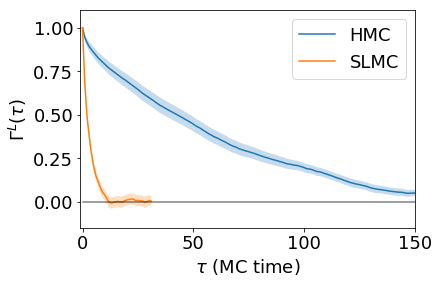
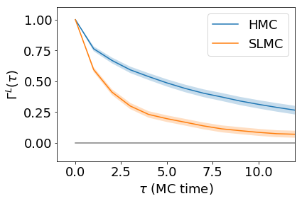
Before detail comparison, we compare HMC and SLMC for $\beta=2.5$, $N_{\sigma}^{3}\times N_{\tau}=6^{4}$, $\hat{m}=0.5$ (Fig.1). The horizontal axis (MC time) is counted as the number of the Metropolis test as we explained above. The integrated autocorrelation time for HMC and SLMC are $\tau^{\text{HMC}}=62(24)$ and $\tau^{\text{SLMC}}=4.0(4)$, respectively. We choose the number of overrelaxation as 10 and the number of heatbath as 100 in this case.

Figure 1: Autocorrelation function for the Polyakov loop for $\beta=2.5$, $N_{\sigma}^{3}\times N_{\tau}=6^{4}$, $\hat{m}=0.5$. We measure the Monte-Carlo time $\tau$ as a unit of the Metropolis test. The bands indicate one sigma error bar. Please see main text for meaning of the horizontal axis.

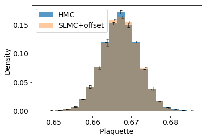
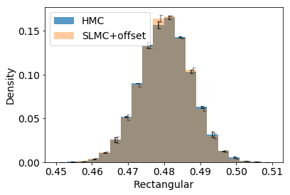
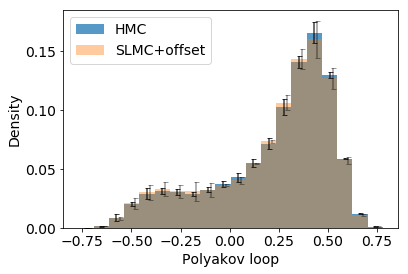
We show results from HMC and SLMC for plaquette, rectangular Wilson loop, and Polyakov loop in histogram with statistical error in Fig.2. One can see that all quantities from SLMC are consistent with ones from HMC. The shape of the histogram for the Polyakov loop indicates the effects of dynamical fermions because if it is quenched, the Polyakov loop is symmetric under $\mathbb{Z}_{2}$ reflection if the statistics are large enough.

Figure 2: Histogram of results from HMC and SLMC for $\beta=2.5$, $N_{\sigma}^{3}\times N_{\tau}=6^{4}$, $\hat{m}=0.5$. To distinguish these results, we shift results for SLMC to the right. Error bar is estimated by the Jackknife method. (Left) Plaquette. (Middle) Rectangular Wilson loop. (Right) Polyakov loop.

Other quantities and setups are summarized the results in Tab.1. ID 0–7 in the table are results from HMC and various SLMC with $N_{\sigma}^{3}\times N_{\tau}=6^{4}$, $\beta=2.5$, and $\hat{m}=0.5$. SLMC_nup100 means SLMC with 100 times heatbath update. SLMC_all means that SLMC with effective action, including $3\times 1$-rectangular, chair, and crown operators. SLMCnor01 and SLMCnor20 mean SLMC with 1 and 20 time overrelaxation after the heatbath update, respectively. SLMCplq means SLMC with an effective action, which includes only plaquette term. SLMCplqrct means SLMC with an effective action, which includes plaquette and the rectangular term. All of the results from various SLMC are consistent with ones from HMC, as expected. Besides, SLMCplq contains only one term, but it achieves roughly 60 % acceptance and with consistent results. Comparing to the acceptance rate for SLMCplqrct and SLMC_all, improvement of effective action, namely adding more loop operators, the data shows that adding loops improves the acceptance rate.

Beta dependence are summarized in ID 8–13 in Tab.1. We vary $\beta$ as $0.8,1.2,4.0$ both in HMC and SLMC. The acceptance rate in SLMC for $\beta=0.8$ is slightly low, but it gives consistent results. $\beta$ dependence is correctly reproduced.

Results from lighter mass $\hat{m}=0.05$ are summarized in ID 14–16 in Tab.1. In this case, for SLMC, acceptance is low (30-40%), but it still gives consistent results to the ones in HMC. The acceptance rate for SLMC_polys (effective action with char, crown, and $3\times 1$ Wilson loop) is improved from SLMC. ID 17–18 in the table are results for $\hat{m}=0.1$. The tendency of acceptance rate is the same to $\hat{m}=0.05$ but slightly better as expected.

We examine volume dependence in the table (ID 19–21) and the volume is taken to $N_{\sigma}^{3}\times N_{\tau}=8^{4}$. Acceptance rate is lower than the SLMC with $N_{\sigma}^{3}\times N_{\tau}=6^{4}$. This is similar to what happens for the reweighting, but in our case, thanks to the tunable parameters, inefficiency is not drastic. Examinations for smaller volume $N_{\sigma}^{3}\times N_{\tau}=4^{4}$ are summarized in ID 22–23. The acceptance rate reaches to 80% for SLMC, and this is also expected.

In summary, SLMC can reproduce results from HMC even with plaquette effective action. The number of terms in the effective action affects to acceptance rate. For larger volumes and small mass, the acceptance rate becomes small. This can be improved by adding more and more terms to the effective action.

ID	ALG	$N_{\sigma}$	$N_{\tau}$	$\beta$	$m$	Acceptance	$N_{\text{trj}}$	$\left\langle P\right\rangle$	$\left\langle R\right\rangle$	$\left\langle L\right\rangle$
0	HMC	6	6	2.5	0.50	0.65	50000	0.66718(5)	0.48037(9)	0.23(1)
1	SLMC_nup100	6	6	2.5	0.50	0.72	48850	0.66711(1)	0.48021(3)	0.197(3)
2	SLMC	6	6	2.5	0.50	0.73	50000	0.66718(3)	0.48031(5)	0.22(1)
3	SLMC_all	6	6	2.5	0.50	0.77	50000	0.66719(3)	0.48034(5)	0.19(1)
4	SLMCnor01	6	6	2.5	0.50	0.74	50000	0.66717(3)	0.48032(5)	0.23(2)
5	SLMCnor20	6	6	2.5	0.50	0.73	50000	0.66731(3)	0.48054(4)	0.191(9)
6	SLMCplq	6	6	2.5	0.50	0.57	50000	0.66746(4)	0.48074(5)	0.18(1)
7	SLMCplqrct	6	6	2.5	0.50	0.69	50000	0.66727(5)	0.48046(7)	0.211(8)
8	HMC	6	6	0.8	0.50	0.85	50000	0.20764(4)	0.04444(3)	0.0025(3)
9	HMC	6	6	1.2	0.50	0.84	50000	0.30356(4)	0.09382(3)	0.0034(2)
10	HMC	6	6	4.0	0.50	0.73	50000	0.80346(3)	0.68011(4)	0.65(1)
11	SLMC	6	6	0.8	0.50	0.58	50000	0.20781(5)	0.04454(5)	0.0032(4)
12	SLMC	6	6	1.2	0.50	0.59	50000	0.30365(4)	0.09387(3)	0.0033(7)
13	SLMC	6	6	4.0	0.50	0.87	50000	0.8035(2)	0.68016(3)	0.58(4)
14	HMC	6	6	2.5	0.05	0.82	50000	0.67774(4)	0.49772(5)	0.437(6)
15	SLMC	6	6	2.5	0.05	0.34	50000	0.67813(8)	0.4982(1)	0.436(7)
16	SLMC_polys	6	6	2.5	0.05	0.43	36350	0.67793(4)	0.49798(5)	0.446(7)
17	HMC	6	6	2.5	0.10	0.73	50000	0.6771(4)	0.49666(5)	0.428(6)
18	SLMC	6	6	2.5	0.10	0.37	50000	0.67749(7)	0.49732(9)	0.438(5)
19	HMC	8	8	2.5	0.50	0.77	50000	0.66659(2)	0.47916(2)	0.01(1)
20	SLMC	8	8	2.5	0.50	0.54	6630	0.66682(10)	0.4795(2)	-0.03(4)
21	SLMC_all	8	8	2.5	0.50	0.62	5300	0.66678(9)	0.4794(1)	0.04(3)
22	HMC	4	4	2.5	0.50	0.66	50000	0.6706(1)	0.4878(2)	0.64(2)
23	SLMC	4	4	2.5	0.50	0.84	50000	0.67073(7)	0.48792(9)	0.656(7)

Table 1: Simulation results for zero temperature with HMC and SLMC. ALG indicates different algorithms, and please see the main text for details. $\hat{m}$ indicates dimensionless quark mass. Acceptance means the acceptance rate. $N_{\text{trj}}$ is the number of trajectories except for the thermalization. $\left\langle P\right\rangle$, $\left\langle R\right\rangle$, and $\left\langle L\right\rangle$ mean expectation value of plaquette, rectangular Wilson loop, and the Polyakov loop, respectively.

V Application to finite temperature

V.1 Simulation setup

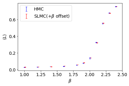
Here we present an application of SLMC algorithm to a finite temperature system. We perform simulation for four flavor QC₂D with $\hat{m}=0.5$ in $N_{\sigma}^{3}\times N_{\tau}=8^{3}\times 4$ lattice. As we will mention later, quarks are not decoupled from the theory. Our $\beta$ range is $\beta=1$ – $2.4$, which contains a transition (crossover) point $\beta_{c}\sim 2.1$. We employ the Wilson plaquette gauge action and the standard staggered fermion. In SLMC update, 20 times heatbath updates are used except for $\beta=2.1$ while 100 times heatbath for $\beta=2.1$. The number of trajectory for HMC are 1000 for $\beta\neq 2.1$ and 20000 for $\beta=2.1$ to see behavior of the Binder cumulant in detail. The number of trajectory for SLMC are O(5000)–O(40000) and please find details in Tab.2.

At the heavy quark mass regime, the system expected to show confinement/deconfinement transition (or crossover) associated with the Polyakov loop. The Polyakov loop operator, along with the imaginary time direction, has the center symmetry, but it is broken at high temperatures. It means that the system around or above the (pseudo-)critical temperature, the system could be affected by long autocorrelation for the Polyakov loop. We attempt to solve this autocorrelation by employing SLMC. Meanwhile, we show that SLMC with effective action can treat detail of phase transition without bias.

V.2 Simulation results

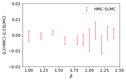
Here we show results at finite temperature. At the heavy mass regime, Polyakov loop is a central observable. Polyakov loop as a function of $\beta$ is shown in left panel of Fig.3 One can see that a transition point is around $\beta\sim 2.1$. Right panel of Fig.3 is difference of results for the Polyakov loop from HMC and SLMC and the values are consistent with 0. Central values for other gluonic observables can be found in Tab.2.

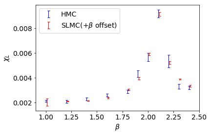
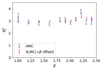
Next, we show results for the susceptibility for Polyakov loop (left panel of Fig.4). One can find a peak of around $\beta\sim 2.1$. Besides, results from HMC and SLMC are consistent with each other. Right panel of Fig.4 is the Binder cumulant for Polyakov loop. Results from HMC and SLMC are consistent with each other. Besides, the Binder cumulant suggest that our quark mass $\hat{m}=0.5$ is not in the quenched regime because in the quenched case, it takes a value for the second-order phase transition $B^{4}_{L}\approx 1.6$ [59, 60].

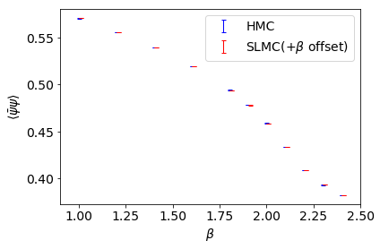
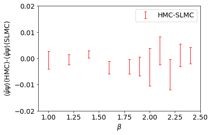
Next, we show results for the chiral condensates as a function of $\beta$ (Left panel of Fig.5). The transition point is located $\beta\sim 2.1$. Right panel of Fig.5 is difference of results for the chiral condensates from HMC and SLMC. Results show that central values are consistent with each other.

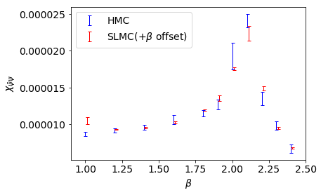
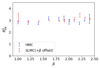
Results of higher cumulants can be found in Fig.6. Left panel of Fig.6 shows the susceptibility for the chiral condensates while the right panel is Binder cumulant for the chiral condensates. Results from HMC and SLMC are consistent with each other.

Our results of the Binder cumulant for the Polyakov loop and chiral condensates (Fig.4 and Fig.6) at $\hat{m}=0.5$ do not show any indication of the second order (with three-dimensional Ising universality class). This can be confirmed by performing a systematic study for large volumes, a finer scan of beta, and increasing statistics, but we leave this issue for a future study.

ID	ALG	$N_{\sigma}$	$N_{\tau}$	$\beta$	$m$	Acceptance	$N_{\text{trj}}$	$\left\langle P\right\rangle$	$\left\langle R\right\rangle$	$\left\langle L\right\rangle$
0	HMC	8	4	1.0	0.5	0.88	1000	0.256(2)	0.067(1)	0.028(2)
1	HMC	8	4	1.2	0.5	0.89	1000	0.3037(2)	0.0939(1)	0.031(2)
2	HMC	8	4	1.4	0.5	0.87	1000	0.353(2)	0.1269(2)	0.036(1)
3	HMC	8	4	1.6	0.5	0.87	1000	0.4048(3)	0.1674(3)	0.039(2)
4	HMC	8	4	1.8	0.5	0.85	1000	0.4625(3)	0.2204(3)	0.055(3)
5	HMC	8	4	1.9	0.5	0.85	1000	0.4948(3)	0.2541(4)	0.078(3)
6	HMC	8	4	2.0	0.5	0.85	1000	0.5297(5)	0.2942(7)	0.137(7)
7	HMC	8	4	2.1	0.5	0.85	20200	0.5684(2)	0.3439(3)	0.327(4)
8	HMC	8	4	2.2	0.5	0.84	1000	0.6041(5)	0.3932(8)	0.553(6)
9	HMC	8	4	2.3	0.5	0.85	1000	0.6302(4)	0.4296(6)	0.679(4)
10	HMC	8	4	2.4	0.5	0.85	1000	0.6507(4)	0.4579(6)	0.757(3)
11	SLMC	8	4	1.0	0.5	0.44	990	0.2559(3)	0.0671(3)	0.028(3)
12	SLMC	8	4	1.2	0.5	0.47	41020	0.30368(6)	0.09393(7)	0.0319(5)
13	SLMC	8	4	1.4	0.5	0.48	41930	0.35296(7)	0.12676(7)	0.0347(5)
14	SLMC	8	4	1.6	0.5	0.46	41970	0.40492(5)	0.16744(6)	0.0424(5)
15	SLMC	8	4	1.8	0.5	0.47	41570	0.46257(7)	0.2205(8)	0.0578(7)
16	SLMC	8	4	1.9	0.5	0.47	5590	0.4949(3)	0.2544(4)	0.081(2)
17	SLMC	8	4	2.0	0.5	0.46	41200	0.53001(7)	0.2947(1)	0.14(1)
18	SLMCup100	8	4	2.1	0.5	0.41	11920	0.5682(2)	0.3437(3)	0.324(3)
19	SLMC	8	4	2.2	0.5	0.50	41180	0.6049(8)	0.3944(1)	0.559(1)
20	SLMC	8	4	2.3	0.5	0.55	34670	0.63037(4)	0.42958(6)	0.6775(6)
21	SLMC	8	4	2.4	0.5	0.60	34550	0.65066(3)	0.45782(4)	0.7558(5)

Table 2: Same table with Tab.1 but for finite temperature with HMC and SLMC.

Figure 3: Polyakov loop as a function of $\beta$. To avoid overlapping of symbols, we slightly shift in $\beta$ for SLMC to the right in plots. (Left) Comparison plot for HMC and SLMC. (Right) Difference between Polyakov loop by HMC and SLMC.

Figure 4: Susceptibility and the Binder cumulant for Polyakov loop as a function of $\beta$. To avoid overlapping symbols, we shift $\beta$ for SLMC in plots. (Left) Polyakov loop susceptibility. It has a peak $\beta\sim 2.1$. (Right) The Binder cumulant. It takes values about $3$ for all $\beta$ regime.

Figure 5: Same plots of Fig.3 but for the chiral condensate.

Figure 6: Same plots of Fig.4 but for the chiral condensate.

As we have seen, $\beta=2.1$ is closes coupling to the critical (crossover) point. Fig.7. We choose the number of heatbath update as 100 in this case.

Figure 7: Autocorrelation function for the Polyakov loop for $\beta=2.1$, $N_{\sigma}^{3}\times N_{\tau}=8^{3}\times 4$, $\hat{m}=0.5$. the number of the heatbath is 100 in SLMC.

VI Conclusion

In this work, we develop self-learning Monte-Carlo algorithm for lattice Yang-Mills theory with dynamical fermions in four dimensions. We work with QC₂D with $n_{f}=4$ as an example with zero and finite temperature.

We confirm that SLMC works for zero temperature runs even for the out of expansion radius of the hopping parameter expansion because of the exactness. This is expected since SLMC itself is free from the choice of effective action. The acceptance rate becomes low for small $\beta$ and large volume, but it can be fixed by adding more extended loops. Our code for automatic generation of heatbath code will be published in another paper.

For finite temperature runs, we confirm that SLMC reproduces correct results with HMC, including higher-order moments of the Polyakov loop and the chiral condensate. Our calculations indicate that QC₂D with $\hat{m}=0.5$ is in the crossover regime, and we leave the precise determination of the order of phase transition to future study.

Our current algorithm uses heavy mass expanded effective action with the linear regression, which induces low efficiency of simulation for lighter mass. This would be fixed by employing a neural network like [34].

References

- [1] M. Creutz. Monte Carlo Study of Quantized SU(2) Gauge Theory. Phys. Rev. D, 21:2308–2315, 1980.
- [2] S. Aoki et al. FLAG Review 2019: Flavour Lattice Averaging Group (FLAG). Eur. Phys. J. C, 80(2):113, 2020.
- [3] Kohtaroh Miura. Review of Lattice QCD Studies of Hadronic Vacuum Polarization Contribution to Muon . PoS, LATTICE2018:010, 2019.
- [4] A.D. Kennedy. Algorithms for dynamical fermions. 7 2006.
- [5] Simon Duane, A.D. Kennedy, Brian J. Pendleton, and Duncan Roweth. Hybrid monte carlo. Physics Letters B, 195(2):216 – 222, 1987.
- [6] M.A. Clark. The Rational Hybrid Monte Carlo Algorithm. PoS, LAT2006:004, 2006.
- [7] Stefan Schaefer, Rainer Sommer, and Francesco Virotta. Critical slowing down and error analysis in lattice QCD simulations. Nucl. Phys. B, 845:93–119, 2011.
- [8] B.A. Berg and T. Neuhaus. Multicanonical ensemble: A New approach to simulate first order phase transitions. Phys. Rev. Lett., 68:9–12, 1992.
- [9] Heng-Tong Ding, Christian Schmidt, Akio Tomiya, and Xiao-Dan Wang. Chiral phase structure of three flavor QCD in a background magnetic field. Phys. Rev. D, 102(5):054505, 2020.
- [10] Pankaj Mehta, Marin Bukov, Ching-Hao Wang, Alexandre G.R. Day, Clint Richardson, Charles K. Fisher, and David J. Schwab. A high-bias, low-variance introduction to machine learning for physicists. Physics Reports, 810:1–124, May 2019.
- [11] Akinori Tanaka and Akio Tomiya. Detection of phase transition via convolutional neural networks. Journal of the Physical Society of Japan, 86(6):063001, Jun 2017.
- [12] Stefan Blücher, Lukas Kades, Jan M. Pawlowski, Nils Strodthoff, and Julian M. Urban. Towards novel insights in lattice field theory with explainable machine learning. Phys. Rev. D, 101(9):094507, 2020.
- [13] Boram Yoon. Estimation of matrix trace using machine learning, 2016.
- [14] Boram Yoon, Tanmoy Bhattacharya, and Rajan Gupta. Machine learning estimators for lattice qcd observables. Physical Review D, 100(1), Jul 2019.
- [15] Rui Zhang, Zhouyou Fan, Ruizi Li, Huey-Wen Lin, and Boram Yoon. Machine-learning prediction for quasiparton distribution function matrix elements. Physical Review D, 101(3), Feb 2020.
- [16] Kim A. Nicoli, Christopher J. Anders, Lena Funcke, Tobias Hartung, Karl Jansen, Pan Kessel, Shinichi Nakajima, and Paolo Stornati. On estimation of thermodynamic observables in lattice field theories with deep generative models, 2020.
- [17] Akinori Tanaka and Akio Tomiya. Towards reduction of autocorrelation in hmc by machine learning, 2017.
- [18] Jan M Pawlowski and Julian M Urban. Reducing autocorrelation times in lattice simulations with generative adversarial networks. Machine Learning: Science and Technology, 1(4):045011, Oct 2020.
- [19] Kai Zhou, Gergely Endrodi, Long-Gang Pang, and Horst Stocker. Regressive and generative neural networks for scalar field theory. Physical Review D, 100(1), Jul 2019.
- [20] M. S. Albergo, G. Kanwar, and P. E. Shanahan. Flow-based generative models for markov chain monte carlo in lattice field theory. Physical Review D, 100(3), Aug 2019.
- [21] Gurtej Kanwar, Michael S. Albergo, Denis Boyda, Kyle Cranmer, Daniel C. Hackett, Sebastien Racaniere, Danilo Jimenez Rezende, and Phiala E. Shanahan. Equivariant flow-based sampling for lattice gauge theory. Physical Review Letters, 125(12), Sep 2020.
- [22] Denis Boyda, Gurtej Kanwar, Sebastien Racaniere, Danilo Jimenez Rezende, Michael S. Albergo, Kyle Cranmer, Daniel C. Hackett, and Phiala E. Shanahan. Sampling using gauge equivariant flows, 2020.
- [23] Andrei Alexandru, Paulo F. Bedaque, Henry Lamm, and Scott Lawrence. Deep learning beyond lefschetz thimbles. Physical Review D, 96(9), Nov 2017.
- [24] Phiala E. Shanahan, Daniel Trewartha, and William Detmold. Machine learning action parameters in lattice quantum chromodynamics. Physical Review D, 97(9), May 2018.
- [25] Lukas Kades, Jan M. Pawlowski, Alexander Rothkopf, Manuel Scherzer, Julian M. Urban, Sebastian J. Wetzel, Nicolas Wink, and Felix Ziegler. Spectral reconstruction with deep neural networks, 2019.
- [26] Boram Yoon, Tanmoy Bhattacharya, and Rajan Gupta. Machine learning estimators for lattice qcd observables, 2019.
- [27] Sam Offler, Gert Aarts, Chris Allton, Jonas Glesaaen, Benjamin Jager, Seyong Kim, Maria Paola Lombardo, Sinead M. Ryan, and Jon-Ivar Skullerud. News from bottomonium spectral functions in thermal qcd, 2019.
- [28] Rui Zhang, Carson Honkala, Huey-Wen Lin, and Jiunn-Wei Chen. Pion and kaon distribution amplitudes in the continuum limit, 2020.
- [29] D. L. Boyda, M. N. Chernodub, N. V. Gerasimeniuk, V. A. Goy, S. D. Liubimov, and A. V. Molochkov. Machine-learning physics from unphysics: Finding deconfinement temperature in lattice yang-mills theories from outside the scaling window, 2020.
- [30] Yarin Gal, Vishnu Jejjala, Damian Kaloni Mayorga Pena, and Challenger Mishra. Baryons from mesons: A machine learning perspective, 2020.
- [31] Sebastian Johann Wetzel and Manuel Scherzer. Machine Learning of Explicit Order Parameters: From the Ising Model to SU(2) Lattice Gauge Theory. Phys. Rev. B, 96(18):184410, 2017.
- [32] Junwei Liu, Yang Qi, Zi Yang Meng, and Liang Fu. Self-learning monte carlo method. Physical Review B, 95(4), Jan 2017.
- [33] Yuki Nagai, Huitao Shen, Yang Qi, Junwei Liu, and Liang Fu. Self-learning Monte Carlo method: Continuous-time algorithm. Physical Review B, 96(16):161102, oct 2017.
- [34] Huitao Shen, Junwei Liu, and Liang Fu. Self-learning monte carlo with deep neural networks. Physical Review B, 97(20), May 2018.
- [35] Chuang Chen, Xiao Yan Xu, Junwei Liu, George Batrouni, Richard Scalettar, and Zi Yang Meng. Symmetry-enforced self-learning Monte Carlo method applied to the Holstein model. Physical Review B, 98(4):1–6, 2018.
- [36] Yuki Nagai, Masahiko Okumura, Keita Kobayashi, and Motoyuki Shiga. Self-learning hybrid monte carlo: A first-principles approach. Physical Review B, 102(4), Jul 2020.
- [37] Junwei Liu, Huitao Shen, Yang Qi, Zi Yang Meng, and Liang Fu. Self-Learning Monte Carlo Method in Fermion Systems. (1):1–5, 2016.
- [38] Yuki Nagai, Masahiko Okumura, Keita Kobayashi, and Motoyuki Shiga. Self-learning hybrid Monte Carlo: A first-principles approach. Physical Review B, 102(4):41124, 2020.
- [39] Alan C. Irving and James C. Sexton. Approximate actions for lattice qcd simulation. Physical Review D, 55(9):5456–5473, May 1997.
- [40] Alan C. Irving, James C. Sexton, and Eamonn Cahill. Approximate actions for dynamical fermions. Nuclear Physics B - Proceedings Supplements, 63(1-3):967–969, Apr 1998.
- [41] A. Duncan, E. Eichten, and H. Thacker. Efficient algorithm for qcd with light dynamical quarks. Physical Review D, 59(1), Nov 1998.
- [42] A. Duncan, E. Eichten, and H. Thacker. Truncated determinant approach to light dynamical quarks. Nuclear Physics B - Proceedings Supplements, 73(1-3):837–839, Mar 1999.
- [43] A. Duncan, E. Eichten, R. Roskies, and H. Thacker. Loop representations of the quark determinant in lattice qcd. Physical Review D, 60(5), Jul 1999.
- [44] Martin Hasenbusch. Exploiting the hopping parameter expansion in the hybrid monte carlo simulation of lattice qcd with two degenerate flavors of wilson fermions. Physical Review D, 97(11), Jun 2018.
- [45] A. Borrelli, Ph. de Forcrand, and A. Galli. Non-hermitian exact local bosonic algorithm for dynamical quarks. Nuclear Physics B, 477(3):809– 832, Oct 1996.
- [46] C. Alexandrou, Ph. de Forcrand, M. D’Elia, and H. Panagopoulos. Improved multiboson algorithm. Nuclear Physics B - Proceedings Supplements, 83-84:765–767, Apr 2000.
- [47] O. Kaczmarek, F. Karsch, and E. Laermann. Thermodynamics of two-colour qcd. Nuclear Physics B - Proceedings Supplements, 73(1-3):441–443, Mar 1999.
- [48] Jeff Bezanson, Alan Edelman, Stefan Karpinski, and Viral B Shah. Julia: A fresh approach to numerical computing. SIAM review, 59(1):65–98, 2017.
- [49] A. Tomiya Y. Nagai, A. Tanaka. Julia code for lqcd. In preparation.
- [50] Anna Hasenfratz, Roland Hoffmann, and Stefan Schaefer. Reweighting towards the chiral limit. Physical Review D, 78(1), Jul 2008.
- [51] Thomas DeGrand. Reweighting qcd simulations with dynamical overlap fermions. Physical Review D, 78(11), Dec 2008.
- [52] H. Saito, S. Ejiri, S. Aoki, T. Hatsuda, K. Kanaya, Y. Maezawa, H. Ohno, and T. Umeda. Phase structure of finite temperature qcd in the heavy quark region. Physical Review D, 84(5), Sep 2011.
- [53] Thomas Blum, Taku Izubuchi, and Eigo Shintani. New class of variance-reduction techniques using lattice symmetries. Physical Review D, 88(9), Nov 2013.
- [54] Sourendu Gupta, A. Irback, F. Karsch, and B. Petersson. The Acceptance Probability in the Hybrid Monte Carlo Method. Phys. Lett. B, 242:437–443, 1990.
- [55] Kurt Binder. Critical properties from monte carlo coarse graining and renormalization. Physical Review Letters, 47(9):693, 1981.
- [56] Ulli Wolff. Monte Carlo errors with less errors. Comput. Phys. Commun., 156:143–153, 2004. [Erratum: Comput. Phys. Commun.176,383(2007)].
- [57] Neal Madras and Alan D. Sokal. The Pivot algorithm: a highly efficient Monte Carlo method for selfavoiding walk. J. Statist. Phys., 50:109–186, 1988.
- [58] Martin Luscher. Schwarz-preconditioned HMC algorithm for two-flavour lattice QCD. Comput. Phys. Commun., 165:199–220, 2005.
- [59] J. Engels, J. Fingberg, and M. Weber. Finite Size Scaling Analysis of SU(2) Lattice Gauge Theory in (3+1)-dimensions. Nucl. Phys. B, 332:737–759, 1990.
- [60] A. Denbleyker, Yuzhi Liu, Y. Meurice, and A. Velytsky. Finite size scaling and universality in su(2) at finite temperature, 2009.
- [61] Benjamin Svetitsky and Laurence G. Yaffe. Critical Behavior at Finite Temperature Confinement Transitions. Nucl. Phys. B, 210:423–447, 1982.
- [62] Robert D. Pisarski and Frank Wilczek. Remarks on the Chiral Phase Transition in Chromodynamics. Phys. Rev. D, 29:338–341, 1984.