Solving Trust Region Subproblems Using Riemannian Optimization

Abstract

The Trust Region Subproblem is a fundamental optimization problem that takes a pivotal role in Trust Region Methods. However, the problem, and variants of it, also arise in quite a few other applications. In this article, we present a family of iterative Riemannian optimization algorithms for a variant of the Trust Region Subproblem that replaces the inequality constraint with an equality constraint, and converge to a global optimum. Our approach uses either a trivial or a non-trivial Riemannian geometry of the search-space, and requires only minimal spectral information about the quadratic component of the objective function. We further show how the theory of Riemannian optimization promotes a deeper understanding of the Trust Region Subproblem and its difficulties, e.g., a deep connection between the Trust Region Subproblem and the problem of finding affine eigenvectors, and a new examination of the so-called hard case in light of the condition number of the Riemannian Hessian operator at a global optimum. Finally, we propose to incorporate preconditioning via a careful selection of a variable Riemannian metric, and establish bounds on the asymptotic convergence rate in terms of how well the preconditioner approximates the input matrix.

1 Introduction

In this paper, we consider the solution of the following problem, which we term as the Boundary Trust Region Subproblem (btrs):

(1) $$\min q\left({\mathbf{x}}\right)\coloneqq\frac{1}{2}{\mathbf{x}}^{\textsc{T}}{\bm{\mathrm{A}}}{\mathbf{x}}+{\mathbf{b}}^{\textsc{T}}{\mathbf{x}}\,\,\,\text{s.t.}\,\,\,\|{\mathbf{x}}\|_{2}=1,$$

where ${\bm{\mathrm{A}}}\in\mathbb{R}^{n\times n}$ is symmetric and ${\mathbf{b}}\in\mathbb{R}^{n}$. btrs is closely related to the well known Trust Region Subproblem (trs), which arises in Trust Region Methods:

(2) $$\min q\left({\mathbf{x}}\right)\,\,\,\text{s.t.}\,\,\,\|{\mathbf{x}}\|_{2}\leq 1.$$

Indeed, btrs (Eq. 1) simply replaces the inequality constraints $\|{\mathbf{x}}\|_{2}\leq 1$ with the equality constraints $\|{\mathbf{x}}\|_{2}=1$. Clearly, these problems coincide whenever a solution for trs can be found on the boundary. Furthermore, an algorithm for solving btrs can be used as a component in an algorithm to solve trs, e.g., in [2]. Alternatively, a simple augmentation trick can be used to translate an $n$ dimensional trs to an equivalent $n+1$ dimensional btrs [24].

While the solution of trs was the initial motivation for our study, our study is also well motivated by the fact that btrs arises in quite a few applications. Indeed, btrs is a form of a constrained eigenvalue problem [12] that, in turn, arises in machine learning applications such as transductive learning [17], semi-supervised support vector machines [9], etc. It also arises when solving quadratically constrained least squares problems [13], which are closely related to ridge regression. Phan et al. discussed applications of btrs in the context of constrained linear regression and tensor decomposition [24]. Finally, we mention recent work on robust function estimation with applications to phase unwrapping [10].

In many applications, there is a need to solve large-scale instances of btrs or trs, so even if the matrix ${\bm{\mathrm{A}}}$ is accessible and stored in-memory, direct operations such as matrix factorizations are not realistic in terms of running times and/or memory requirements. For this reason, methods that rely solely on matrix-vector products, i.e matrix-free iterative algorithms, are of great interest and appeal when approaching these problems. In this paper we focus on developing matrix-free iterative algorithms for btrs (and trs). We also propose a family of preconditioned iterative algorithms for solving btrs and trs.

The proposed algorithms are based on Riemannian optimization [1], that is, constrained optimization algorithms that utilize smooth manifold structures of constraint sets. Although btrs is a non-convex problem which can have non-global local minimizers, we show that it is possible to find a global solution using an almost trivial modification of standard Riemannian Gradient Descent without any spectral information about the matrix ${\bm{\mathrm{A}}}$ (Section 4). Next, we show that this can be taken one step further, and find a global solution of a btrs with first-order Riemannian algorithms and/or other choices of retraction and/or non-standard Riemannian metric, as long as we have access to the eigenvectors of ${\bm{\mathrm{A}}}$ associated with its smallest eigenvalue (Section 5); a requirement that is computationally feasible.

It is well known that matrix-free iterative methods may suffer from slow convergence rates, and that preconditioning can be effective in improving convergence rates of iterative solvers. Using Riemannian optimization, we are able to perform Riemannian preconditioning [21, 25] by choosing a non-standard [11, Eq. 2.2] metric. Indeed, Riemannian preconditioning introduces a preconditioner by changing the Riemannian metric. We show how to precondition our proposed Riemannian algorithms using an easy-to-factorize approximation ${\bm{\mathrm{M}}}$ of ${\bm{\mathrm{A}}}$. To justify the use of the preconditioner, we present a theoretical analysis that bounds the condition number of the Hessian at the optimum (a useful proxy for assessing convergence rate of Riemannian solvers) in terms of how well ${\bm{\mathrm{M}}}$ approximates ${\bm{\mathrm{A}}}$ (Section 6).

As with any preprocessing, the construction of a preconditioner is expected to have additional computational costs. Our theoretical results are supported by numerical illustrations showing that our preconditioning scheme introduces a speedup large enough in order to result in overall computational costs that are reduced in comparison with iterative schemes based on the standard geometry (Section 8).

1.1 Contributions and organization

Our work is the first to tackle btrs directly using Riemannian optimization, without re-formulating the problem (see Section 2.2). The main contributions established by viewing this problem from the lens of Riemannian optimization are:

• Theoretically, we analyze the possible critical points and their stability, and we explore connections between trs and finding affine eigenvectors using Riemannian optimization theory (Section 3). In addition, we analyze the easy and hard cases (Section 4), and show a theoretical relation between the hard case of btrs and the condition number of the Riemannian Hessian at the optimum (Section 6).

• Algorithmically, we propose to find a global solution of a btrs via a Riemannian optimization algorithm (Section 4). Furthermore, we utilize the technique of Riemannian preconditioning [21], and incorporate preconditioning using a variable Riemannian metric in order to improve the convergence rates of our Riemannian optimization btrs solver (Section 6). Similarly to  [25], we analyze the effect of preconditioning on the asymptotic convergence by establishing bounds on the condition number of the Riemannian Hessian at the optimum. However, unlike in  [25], we propose a variable Riemannian metric which adapts itself as iterations progress. Moreover, we design our preconditioner using minimal spectral information about the quadratic term of the objective function, ${\bm{\mathrm{A}}}$, and using matrix sketching techniques which provide efficient computational costs per iteration compared with the use of the exact matrices. In Section 8, we demonstrate the improvement obtained using our Riemannian preconditioning scheme in comparison with naive Riemannian optimization methods without preconditioning.

From here on, our text is organized as follows: Section 2 contains the related work and preliminaries on Riemannian optimization and preconditioning, in Section 3 we study the stationary points of btrs in the Riemannian optimization framework, in Section 4 we propose an adaptation of Riemannian gradient descent which solves btrs globally, and is suitable both for the easy and hard case of btrs, in Section 5 we widen the class of Riemannian solvers which solve globally btrs and utilize it in Section 6 to construct and analyze a specific preconditioning scheme, in Section 7 we show how to utilize our solution for btrs for achieving a solution for trs, finally in Section 8 we illustrate our algorithms for the easy, "almost hard" and hard cases and demonstrate the effect of preconditioning empirically.

2 Preliminaries

2.1 Notation

We denote scalars by lower case Greek letters without subscripts or using $x,y,z\dots$. Vectors in $\mathbb{R}^{n}$ are denoted by bold lowercase English letters, e.g., ${\mathbf{x}},{\mathbf{y}},{\mathbf{z}}\dots$ and matrices by ${\bm{\mathrm{A}}},{\bm{\mathrm{B}}},{\bm{\mathrm{C}}}\dots$. The $n\times n$ identity matrix will be denoted by ${\bm{\mathrm{I}}}_{n}$ while the subscript is omitted in cases where the dimension is clear from context.

Let ${\bm{\mathrm{A}}}\in\mathbb{R}^{n\times n}$ be a symmetric matrix. We denote its eigenvalues by $\lambda_{1}\left({\bm{\mathrm{A}}}\right)\leq\lambda_{2}\left({\bm{\mathrm{A}}}\right)\leq\dots\leq\lambda_{n}\left({\bm{\mathrm{A}}}\right)$ or simply $\lambda_{i}\leq\lambda_{i+1}$ where the matrix is clear from the context. We also use $\lambda_{\min}$ and $\lambda_{\max}$ to denote the minimal and maximal eigenvalue. For any matrix ${\bm{\mathrm{B}}}\in\mathbb{R}^{n\times n}$, the condition number of ${\bm{\mathrm{B}}}$, denoted by $\kappa({\bm{\mathrm{B}}})$, is defined as the ratio between the largest and smallest singular values of ${\bm{\mathrm{B}}}$. We say that ${\bm{\mathrm{A}}}\in\mathbb{R}^{n\times n}$ is symmetric positive definite matrix (SPD) if ${\bm{\mathrm{A}}}$ is symmetric and all its eigenvalues are strictly positive. In particular, for an SPD matrix, the condition number becomes the ratio between the largest and smallest eigenvalue.

We denote the $n-1$ dimensional sphere in $\mathbb{R}^{n}$ by $\mathbb{S}^{n-1}\coloneqq\{{\mathbf{x}}\in\mathbb{R}^{n}~{}|~{}{\mathbf{x}}^{\textsc{T}}{\mathbf{x}}=1\}$. Recall that $\mathbb{S}^{n-1}$ is a $n-1$ dimensional submanifold of $\mathbb{R}^{n}$. Given a smooth function $f:\mathbb{S}^{n-1}\to\mathbb{R}$, we use the notation $\bar{f}$ to present some smooth extension of $f$ to the entire ambient space of $\mathbb{R}^{n}$, that is, $\bar{f}$ refers to any member of the equivalence class of smooth functions $g:\mathbb{R}^{n}\to\mathbb{R}$ such that $g({\mathbf{x}})=f({\mathbf{x}})$ for all ${\mathbf{x}}\in\mathbb{S}^{n-1}$. We denote the unit norm ball (with respect to the Euclidean norm) in $\mathbb{R}^{n}$ by $\mathbb{B}^{n}$.

Notation within the domain of optimization algorithms on Riemannian manifolds are consistent with the ones in [1], e.g., general manifolds are denoted using calligraphic uppercase English letters $\mathcal{M},\mathcal{N},\dots$. Similarly, for ${\mathbf{x}}\in\mathcal{M}$, the tangent space to $\mathcal{M}$ at ${\mathbf{x}}$ is denoted by $T_{{\mathbf{x}}}{\mathcal{M}}$, and tangent vectors are denoted by lowercase greek letters with a subscript referring the point for which they correspond, e.g., $\eta_{{\mathbf{x}}}\in T_{{\mathbf{x}}}{\mathcal{M}}$.

2.2 Related work

Due to its pivotal role in Trust Region Methods, there has been extensive work on solving trs. There is a variety of classical algorithms to approximate trs solution such as the Cauchy-point algorithm, the dogleg method, two-dimensional subspace minimization and Steihaug’s CG algorithm (see [23, Chapter 4.1] and citations therein). Worth nothing is the seminal work of Moré and Sorensen [22], relating solutions of trs to roots of a secular equation. Another classical algorithm for solving trs at large-scale is based on the Lanczos method [14].

Recent work by Carmon and Duchi on trs include an analysis of the convergence rate of the Lanczos method  [7]. They also prove lower bounds on the computational cost for any deterministic iterative method, accessing ${\bm{\mathrm{A}}}$ only through matrix-vector products and for which each iteration involves only a single product (i.e., matrix-free algorithms). Beck and Vaisbourd proposed to find global solutions of trss by means of first order conic methods (focm) [4], and formulated sufficient conditions for such schemes to converge to the global trs minimizer both in easy and hard cases.

Most previous work on btrs was motivated by trs. Such works addresses btrs only for the special case where the solutions for both problems coincide. However, there are a few exceptions. Martínez characterized local minimizers of btrs and trs [20] and proposed an algorithm for finding a local but non-global minimizer for btrs, when it exists. This characterization is of importance when discussing first-order iterative methods as they usually guarantee convergence to a stationary point without any way to distinguish global from local non-global minimizers. Given a stationary point of btrs other than its global solution, Lucidi et al. presented a transformation (mapping from a vector to another) for finding a point on the sphere for which the objective value is lower [18]. If we use a descent algorithm, Lucidi et al.’s transformation allows us to continue the iteration after converging to a local non-global minimizer (or to any other stationary point). Hager presented an algorithm for solving btrs using a method based on a combination of Newton and Lanczos iterations for Krylov subspace minimization [15]. Adachi et al. proposed to solve btrs by solving a Generalized Eigenvalue Problem of dimension $2n\times 2n$  [2]. Phan et al. proposed an algorithm for solving btrs, however their algorithm requires a full eigendecomposition of ${\bm{\mathrm{A}}}$ [24].

Our proposed algorithm differs from the aforementioned works in three fundamental ways: 1) We consider the use of Riemannian optimization for trs. The only previous work that considered Riemannian optimization for btrs is a recent work by Boumal et al. [5], which considers a semidefinite program relaxation which is followed by a Burer-Monteiro relaxation. Their reformulated problem is an optimization problem constrained on two spheres, an $n\times p$ dimensional sphere and a $p$ dimensional sphere, where $p\geq 2$ is a rank parameter [5, Section 5.2]. Unlike [5], we solve btrs directly via Riemannian optimization. 2) Consequently, for trs, our algorithm seeks the solution of an equivalent $n+1$ dimensional btrs, from which it is trivial to extract the solution for the original trs. 3) We incorporate a preconditioner through the approach of Riemannian preconditioning [21], and not via change-of-variables or preconditioning the solution of linear systems encountered during the optimization (e.g., [27]). Unlike [21], we motivate the design of our preconditioner via the condition number of the Riemannian Hessian at the optimum.

2.3 Riemannian Optimization

Our proposed algorithms use Riemannian optimization for finding the optimal solution of btrs. The framework of Riemannian optimization naturally arises when solving optimization problems in which the search space is a smooth manifold [1, Chapter 3.1]. In this section we recall some basic definitions of Riemannian optimization, and establish corresponding notation. The definitions and notation here are consistent with the ones in [1].

A smooth Riemannian manifold is a differentiable manifold $\mathcal{M}$, equipped with a smoothly varying inner product $g_{{\mathbf{x}}}$ operating on the manifold’s tangent bundle $T\mathcal{M}$, i.e., for any ${\mathbf{x}}\in\mathcal{M}$ the function $g_{{\mathbf{x}}}:T_{{\mathbf{x}}}{\mathcal{M}}\times T_{{\mathbf{x}}}{\mathcal{M}}\rightarrow\mathbb{R}$ is a bilinear function on the tangent space to the manifold $\mathcal{M}$ at point ${\mathbf{x}}$. In turn, this inner product endows a metric function over the tangent space at each point. This inner product is termed the Riemannian metric.

Riemannian optimization algorithms are derived by generalizing various algorithmic components used in non-Riemannian optimization, and as such are naturally defined on $\mathbb{R}^{n}$, to the case of optimization on Riemannian manifolds. For example, a retraction [1, Section 4.1], which is a map $R_{{\mathbf{x}}}:T_{{\mathbf{x}}}{\cal M}\to{\cal M}$, allows Riemannian optimization algorithms to take a step at point ${\mathbf{x}}\in{\cal M}$ in a direction $\xi_{{\mathbf{x}}}\in T_{{\mathbf{x}}}{\cal M}$. Two mathematical objects that are important for our discussion are the Riemannian gradient and the Riemannian Hessian [1, Section 3.6 and 5.5].

Once these various components are generalized, many optimization algorithms for smooth problems are naturally generalized as well. In [1], Riemannian gradient, line-search, Newton method, trust region, and conjugate gradient (CG) methods are presented. An important example is Riemannian gradient descent, which is given by the following formula:

(3) $$\mathbf{x}_{k+1}=R_{\mathbf{x}_{k}}(-t^{(k)}{\bf grad}f(\mathbf{x}_{k})),$$

where $t^{(k)}$ denotes the $k$’th step size. In the above, ${\bf grad}f(\mathbf{x}_{k})$ is the Riemannian gradient of $f$ at $\mathbf{x}_{k}$. When the step size is chosen via Armijo’s backtracking procedure, it is guaranteed that all the accumulation points of a sequence generated by Riemannian Gradient Descent are stationary points of $f$ on $\mathcal{M}$ (vanishing points of the Riemannian gradient), provided $f$ is at least continuously differentiable [1, Theorem 4.3.1]. In general, henceforth, when we discuss Riemannian Gradient Descent we assume that step sizes are chosen so as to assure that all accumulation points are stationary points (e.g., using Armijo’s backtracking procedure).

2.4 Riemannian Preconditioning on the Sphere

The natural way to define a metric on the sphere $\mathbb{S}^{n-1}$ is by using the standard inner product of its ambient space $\mathbb{R}^{n}$: $\bar{g}_{{\mathbf{x}}}(\eta_{\mathbf{x}},\xi_{\mathbf{x}})\coloneqq\eta^{\textsc{T}}_{\mathbf{x}}\xi_{\mathbf{x}}$. The sphere $\mathbb{S}^{n-1}$, as a Riemannian submanifold of $\mathbb{R}^{n}$, then inherits the metric in a natural way. With this metric, we have $g_{{\mathbf{x}}}(\eta_{\mathbf{x}},\xi_{\mathbf{x}})\coloneqq\eta^{\textsc{T}}_{\mathbf{x}}\xi_{\mathbf{x}}$ where $\eta_{\mathbf{x}},\xi_{\mathbf{x}}\in T_{{\mathbf{x}}}\mathbb{S}^{n-1}$ are given in ambient coordinates.

However, Shustin and Avron noticed that in some cases this particular choice of metric may lead to suboptimal performance of iterative algorithms [25]. For example, when minimizing the Rayleigh quotient defined by an SPD ${\bm{\mathrm{A}}}$, the metric defined by ${\bm{\mathrm{A}}}$ , i.e., $g_{{\mathbf{x}}}(\eta_{\mathbf{x}},\xi_{\mathbf{x}})=\eta^{\textsc{T}}_{\mathbf{x}}{\bm{\mathrm{A}}}\xi_{\mathbf{x}}$, was shown to be advantageous [25, Section 4]. In general, different problems call for the use of metrics for the form $g_{{\mathbf{x}}}(\eta_{\mathbf{x}},\xi_{\mathbf{x}})=\eta^{\textsc{T}}_{\mathbf{x}}{\bm{\mathrm{M}}}\xi_{\mathbf{x}}$ with different ${\bm{\mathrm{M}}}$. As the usage of this metric in Riemannian optimization algorithms requires the ability to solve linear systems involving ${\bm{\mathrm{M}}}$, one often wants an ${\bm{\mathrm{M}}}$ that is both easy to invert and closely approximates some optimal (but computationally expensive) metric, e.g., for minimizing $\min_{{\mathbf{x}}\in\mathbb{S}^{n-1}}{\mathbf{x}}^{\textsc{T}}{\bm{\mathrm{A}}}{\mathbf{x}}$ we want an easy-to-invert ${\bm{\mathrm{M}}}\approx{\bm{\mathrm{A}}}$.

Defining the metric on $\mathbb{S}^{n-1}$ via ${\bm{\mathrm{M}}}$ is an instance of so-called Riemannian Preconditioning [21]. In our preconditioned iterative algorithms for btrs, a preconditioner is incorporated using Riemannian preconditioning, that is, we use Riemannian optimization on $\mathbb{S}^{n-1}$ with a non-standard metric. However, in contrast to the work by Shustin and Avron [25], where the metric is defined by a constant preconditioner ${\bm{\mathrm{M}}}$, our algorithm uses a metric that varies on $\mathbb{S}^{n-1}$, i.e, a function $g_{{\mathbf{x}}}(\eta_{\mathbf{x}},\xi_{\mathbf{x}})=\eta^{\textsc{T}}_{\mathbf{x}}{\bm{\mathrm{M}}}_{\mathbf{x}}\xi_{\mathbf{x}}$, where for each ${\mathbf{x}}\in\mathbb{S}^{n-1}$ the matrix ${\bm{\mathrm{M}}}_{{\mathbf{x}}}$ is an SPD, and as such it defines a valid inner product on the tangent space to $\mathbb{S}^{n-1}$ at ${\mathbf{x}}$, and the mapping ${\mathbf{x}}\mapsto{\bm{\mathrm{M}}}_{{\mathbf{x}}}$ is smooth on the sphere (smoothness is required in order for $(\mathbb{S}^{n-1},g)$ to be a Riemannian manifold).

A summary of Riemannian optimization related objects and their expressions in ambient coordinates is given below in Table 1.

Table 1: Riemannian optimization related ingredients for optimizing on $\mathbb{S}^{n-1}$ with varying metric. Based on [25]. Formulas are given in terms of ambient coordinates. Note that ${\mathbf{x}}\in\mathbb{S}^{n-1}\mapsto{\bm{\mathrm{M}}}_{{\mathbf{x}}}$ is a smooth SPD-valued function. The construction of the objects in the btrs column are given in Section 6

	$\min_{{\mathbf{x}}\in\mathbb{S}^{n-1}}f\left({\mathbf{x}}\right)$	btrs
Tangent space to a point ${\mathbf{x}}\in\mathbb{S}^{n-1}$	$T_{{\mathbf{x}}}\mathbb{S}^{n-1}=\left\{{\mathbf{z}}\in\mathbb{R}^{n}\,:\,{\mathbf{z}}^{\textsc{T}}{\mathbf{x}}=0\right\}$
Retraction	$R_{{\mathbf{x}}}(\xi_{{\mathbf{x}}})\coloneqq\frac{{\mathbf{x}}+\xi_{{\mathbf{x}}}}{\|{\mathbf{x}}+\xi_{{\mathbf{x}}}\|_{2}}$
Riemannian metric	$g_{{\mathbf{x}}}\left(\eta_{\mathbf{x}},\xi_{\mathbf{x}}\right)\coloneqq\eta^{\textsc{T}}_{\mathbf{x}}{\bm{\mathrm{M}}}_{{\mathbf{x}}}\xi_{\mathbf{x}}$
Orthogonal projector on $T_{{\mathbf{x}}}\mathbb{S}^{n-1}$	${\bm{\mathrm{P}}}_{{\mathbf{x}}}\coloneqq\left({\bm{\mathrm{I}}}_{n}-1/({\mathbf{x}}^{\textsc{T}}{\bm{\mathrm{M}}}_{{\mathbf{x}}}^{-1}{\mathbf{x}}){\bm{\mathrm{M}}}_{{\mathbf{x}}}^{-1}{\mathbf{x}}{\mathbf{x}}^{\textsc{T}}\right)$
Vector transport	${\cal T}_{\eta_{{\mathbf{x}}}}(\xi_{{\mathbf{x}}})\coloneqq{\bm{\mathrm{P}}}_{R_{{\mathbf{x}}}(\eta_{{\mathbf{x}}})}(\xi_{{\mathbf{x}}})$
Riemannian gradient	${\bf grad}f({\mathbf{x}})={\bm{\mathrm{P}}}_{{\mathbf{x}}}{\bm{\mathrm{M}}}_{{\mathbf{x}}}^{-1}\nabla\bar{f}\left({\mathbf{x}}\right)$	${\bm{\mathrm{P}}}_{{\mathbf{x}}}{\bm{\mathrm{M}}}_{{\mathbf{x}}}^{-1}({\bm{\mathrm{A}}}{\mathbf{x}}+{\mathbf{b}})$
Riemannian Hessian at stationary $\bar{{\mathbf{x}}}$ (i.e., ${\bf grad}f(\bar{{\mathbf{x}}})=0)$	${\text{{Hess}}\nobreak\hskip 0.35002pt}f(\bar{{\mathbf{x}}})[\eta_{\bar{{\mathbf{x}}}}]={\bm{\mathrm{P}}}_{\bar{{\mathbf{x}}}}{\bm{\mathrm{M}}}_{\bar{{\mathbf{x}}}}^{-1}\left[\nabla^{2}\bar{f}\left(\bar{{\mathbf{x}}}\right)-\bar{{\mathbf{x}}}^{\textsc{T}}\nabla\bar{f}\left(\bar{{\mathbf{x}}}\right)){\bm{\mathrm{I}}}_{n}\right]\eta_{\bar{{\mathbf{x}}}}$	${\bm{\mathrm{P}}}_{\bar{{\mathbf{x}}}}{\bm{\mathrm{M}}}_{\bar{{\mathbf{x}}}}^{-1}\left[{\bm{\mathrm{A}}}-\mu_{\bar{{\mathbf{x}}}}{\bm{\mathrm{I}}}_{n}\right]\eta_{\bar{{\mathbf{x}}}}$

3 Stationarity in the btrs and Riemannian Optimization

Our goal in this section is to understand the set of stationary points of btrs, discuss optimality conditions, and understand how this pertains to solving btrs using plain Riemanniann optimization. Some of the results are closely related to similar results for trs [4], but there are subtle differences.

Recall, that for a Riemannian manifold $\mathcal{M}$, a stationary point ${\mathbf{x}}\in\mathcal{M}$ of a smooth scalar function $f:\mathcal{M}\rightarrow\mathbb{R}$ is a point for which the Riemannian gradient vanishes (${\bf grad}f({\mathbf{x}})=0$) [1]. In this section we analyze stationarity of ${\mathbf{x}}\in\mathbb{S}^{n-1}$ for $q$. Since vanishing points of the Riemanninan gradient are invariant to the choice of the metric (as locally, the Riemannian metric is an inner product on the tangent space), we can analyze stationarity with any Riemannian metric of our choice. In this section, we view $\mathbb{S}^{n-1}$ as a Riemannian submanifold of $\mathbb{R}^{n}$ endowed with the dot product as the Riemannian metric.

The following proposition characterizes the stationary points of btrs. The result is already known  [20, 8, 19, 22]. Nevertheless, we provide a new proof, which is based on Riemannian optimization tools.

Proposition 3.1.

A point ${\mathbf{x}}\in\mathbb{S}^{n-1}$ is a stationary point of btrs if and only if there exists $\mu_{\mathbf{x}}\in\mathbb{R}$ such that

(4) $$({\bm{\mathrm{A}}}-\mu_{\mathbf{x}}{\bm{\mathrm{I}}}){\mathbf{x}}=-{\mathbf{b}}.$$

When such is the case, $\mu_{\mathbf{x}}$ is unique, and

(5) $$\mu_{\mathbf{x}}={\mathbf{x}}^{\textsc{T}}{\bm{\mathrm{A}}}{\mathbf{x}}+{\mathbf{b}}^{\textsc{T}}{\mathbf{x}}.$$

Proof 3.2 (Proof of Proposition 3.1).

Since we are viewing $\mathbb{S}^{n-1}$ as a Riemannian submanifold of $\mathbb{R}^{n}$ equipped with usual dot product, we have

$${\bf grad}q({\mathbf{x}})={\bm{\mathrm{P}}}_{{\mathbf{x}}}\nabla\bar{q}({\mathbf{x}})=({\bm{\mathrm{I}}}_{n}-{\mathbf{x}}{\mathbf{x}}^{\textsc{T}})({\bm{\mathrm{A}}}{\mathbf{x}}+{\mathbf{b}})={\bm{\mathrm{A}}}{\mathbf{x}}+{\mathbf{b}}-({\mathbf{x}}^{\textsc{T}}{\bm{\mathrm{A}}}{\mathbf{x}}+{\mathbf{b}}^{\textsc{T}}{\mathbf{x}}){\mathbf{x}}~{}~{}.$$

In the above, $\nabla\bar{q}({\mathbf{x}})$ is the Euclidean gradient of $\bar{q}$ at ${\mathbf{x}}$, and ${\bm{\mathrm{P}}}_{\mathbf{x}}\coloneqq{\bm{\mathrm{I}}}_{n}-{\mathbf{x}}{\mathbf{x}}^{\textsc{T}}$ is the projection matrix on $T_{{\mathbf{x}}}\mathbb{S}^{n-1}$ with respect to the Euclidean inner product (the dot product). The fact that ${\bf grad}q({\mathbf{x}})={\bm{\mathrm{P}}}_{{\mathbf{x}}}\nabla\bar{q}({\mathbf{x}})$ is due to a generic result on the Riemannian gradient of a function on a Riemannian submanifold [1]. Existence of $\mu_{\mathbf{x}}$ and the formula given for it (Equation 5) now follows by equating ${\bf grad}q({\mathbf{x}})=0$. The converse follows from substituting Equation 5 in Equation 4.

As for uniqueness, if there were two $\mu_{{\mathbf{x}},1}$ and $\mu_{{\mathbf{x}},2}$ for which Equation 4 holds, then obviously $\mu_{{\mathbf{x}},1}{\mathbf{x}}=\mu_{{\mathbf{x}},2}{\mathbf{x}}$. Since ${\mathbf{x}}\in\mathbb{S}^{n-1}$ we have $\mu_{{\mathbf{x}},1}=\mu_{{\mathbf{x}},2}$.

A similar claim holds for trs [4], however for trs we always have $\mu_{\mathbf{x}}\leq 0$ while for btrs it is possible that $\mu_{\mathbf{x}}>0$ (however, this may happen only if ${\bm{\mathrm{A}}}$ is positive definite). The set of pairs $(\mu_{{\mathbf{x}}},{\mathbf{x}})$ where ${\mathbf{x}}$ is stationary point of btrs is exactly the set of KKT pairs for btrs [18]. It is also the case that any stationary point on $\mathbb{S}^{n-1}$ of the associated trs is also a stationary point of btrs, but the converse does not always hold.

In the special case where ${\mathbf{b}}=0$, the btrs’s objective function $q({\mathbf{x}})$ is the Rayleigh quotient, and the stationary points are the eigenvectors. In this case, the stationarity conditions reduce to ${\bm{\mathrm{A}}}{\mathbf{x}}=\mu_{\mathbf{x}}{\mathbf{x}}$, so $\mu_{\mathbf{x}}$ is the corresponding eigenvalue. When ${\mathbf{b}}\neq 0$, we can still view a stationary ${\mathbf{x}}$ as an eigenvector, but of an affine transformation instead of a linear one. Indeed, consider the affine transformation ${\bm{\mathrm{T}}}({\mathbf{v}})={\bm{\mathrm{A}}}{\mathbf{v}}+{\mathbf{b}}$. We have that ${\bm{\mathrm{T}}}({\mathbf{x}})=\mu_{\mathbf{x}}{\mathbf{x}}$, i.e., $(\mu_{\mathbf{x}},{\mathbf{x}})$ behaves like an eigenpair of ${\bm{\mathrm{T}}}$. Furthermore, any affine transformation ${\bm{\mathrm{S}}}:\mathbb{R}^{n}\rightarrow\mathbb{R}^{n}$ can be written as ${\bm{\mathrm{S}}}({\mathbf{v}})={\bm{\mathrm{A}}}_{{\bm{\mathrm{S}}}}{\mathbf{v}}+{\mathbf{b}}_{{\bm{\mathrm{S}}}}$ for some $({\bm{\mathrm{A}}}_{{\bm{\mathrm{S}}}},{\mathbf{b}}_{{\bm{\mathrm{S}}}})$. This motivates the following definition which echoes previous observations, e.g. see [12], regarding the stationary points of btrs.

Definition 3.3 (Affine Eigenpairs).

Let ${\bm{\mathrm{A}}}\in\mathbb{R}^{n\times n}$ and ${\mathbf{b}}\in\mathbb{R}^{n}$. We say that $\mu\in\mathbb{R}$ is an affine eigenvalue of $({\bm{\mathrm{A}}},{\mathbf{b}})$ if there exists an ${\mathbf{x}}\in\mathbb{S}^{n-1}$ such that ${\bm{\mathrm{A}}}{\mathbf{x}}+{\mathbf{b}}=\mu{\mathbf{x}}$. Such ${\mathbf{x}}\in\mathbb{S}^{n-1}$ is the affine eigenvector associated with $\mu$. We call the pair $(\mu,{\mathbf{x}})$ an affine eigenpair.

Let us define $\mu_{\mathbf{x}}\coloneqq{\mathbf{x}}^{\textsc{T}}{\bm{\mathrm{A}}}{\mathbf{x}}+{\mathbf{b}}^{\textsc{T}}{\mathbf{x}}$ for any ${\mathbf{x}}$ (not just stationary ${\mathbf{x}}$). If ${\mathbf{b}}=0$, for any ${\mathbf{x}}\in\mathbb{S}^{n-1}$ the quantity $\mu_{\mathbf{x}}$ is a Rayleigh quotient of ${\bm{\mathrm{A}}}$. Since $\mu_{\mathbf{x}}$ plays a similar role for the affine eigenvalues as the Rayleigh quotient plays for the (regular) eigenvalues, we refer to $\mu_{\mathbf{x}}$ the affine Rayleigh quotient of ${\mathbf{x}}$ with respect to $({\bm{\mathrm{A}}},{\mathbf{b}})$. Like the standard Rayleigh quotient, $\mu_{\mathbf{x}}$ provides the "best guess" for the affine eigenvalue, given an approximate affine eigenvector ${\mathbf{x}}$ since $\mu_{\mathbf{x}}=\arg\min_{\mu}\|{\bm{\mathrm{A}}}{\mathbf{x}}+{\mathbf{b}}-\mu{\mathbf{x}}\|_{2}$.

Corollary 3.4.

A point ${\mathbf{x}}\in\mathbb{S}^{n-1}$ is a stationary btrs point if and only if ${\mathbf{x}}$ is an affine eigenvector of $({\bm{\mathrm{A}}},{\mathbf{b}})$, and its associated affine eigenvalue is the affine Rayleigh quotient $\mu_{{\mathbf{x}}}$.

In their work, Moré and Sorensen have shown that when ${\mathbf{b}}\neq 0$ the affine eigenvalues of $({\bm{\mathrm{A}}},{\mathbf{b}})$ are the roots of a secular equation [22]. As Lucidi et al. later noted, this implies that there is at most one affine eigenvalue smaller or equal to the minimal eigenvalue $\lambda_{1}$ of ${\bm{\mathrm{A}}}$, at most two affine eigenvalues between each two distinct eigenvalues, and exactly one affine eigenvalue larger or equal to the largest eigenvalue $\lambda_{n}$ of ${\bm{\mathrm{A}}}$ [18]. In a sense, when ${\bm{\mathrm{A}}}$ is symmetric there are at most two affine eigenvalues per each regular eigenvalue, one smaller than it and one larger than it. When ${\mathbf{b}}=0$, these two affine eigenvalues coincide and have two different eigenvectors, which are the reflection of each other. When ${\mathbf{b}}$ is perturbed, the affine eigenvectors bifurcate, and when ${\mathbf{b}}$ is large enough there might fail to be a root of the secular equation (and the affine eigenvalue disappears).

The following lemma is a compilation of multiple results from [20, 18] and relates affine eigenpairs to local and global btrs minimizers. Right afterwards we state and prove a refinement of the first clause of the lemma.

Lemma 3.5 (Combining multiple results from [20, 18]).

Let ${\bm{\mathrm{A}}}\in\mathbb{R}^{n\times n}$ be a symmetric matrix and ${\mathbf{b}}\in\mathbb{R}^{n}$. The following statements hold:

1. Any global btrs solution is an affine eigenvector $\mathbf{x_{\star}}$ associated with the smallest affine eigenvalue $\mu_{\star}$ and vice versa. We also have $\mu_{\star}\leq\lambda_{1}({\bm{\mathrm{A}}})$.

2. Any stationary point which is not a global solution is an affine eigenvector $\bar{{\mathbf{x}}}$ associated with an affine eigenvalue $\bar{\mu}$ for which $\bar{\mu}>\lambda_{1}({\bm{\mathrm{A}}})$ .

3. If the minimal eigenvalue of ${\bm{\mathrm{A}}}$ is simple, there are at most two distinct local btrs minimizers [18], otherwise, any local btrs minimizer is a global solution [20, Lemma 2.2].

4. In case ${\mathbf{b}}\perp{\mathbf{u}}$ for some ${\mathbf{u}}\in\mathbb{S}^{n-1}$ such that ${\bm{\mathrm{A}}}{\mathbf{u}}=\lambda_{1}({\bm{\mathrm{A}}}){\mathbf{u}}$, any local btrs minimizer is a global one.

5. Let $\bar{{\mathbf{x}}}\in\mathbb{S}^{n-1}$ be a local but non-global btrs minimizer, then the affine eigenvalue $\bar{\mu}$ associated with $\bar{{\mathbf{x}}}$ is the second smallest affine eigenvalue, with $\lambda_{1}({\bm{\mathrm{A}}})<\bar{\mu}<\lambda_{2}({\bm{\mathrm{A}}})$.

Proposition 3.6.

Suppose that ${{\mathbf{u}}}^{\textsc{T}}{\mathbf{b}}\neq 0$ for some ${\mathbf{u}}\in\mathbb{S}^{n-1}$ such that ${\bm{\mathrm{A}}}{\mathbf{u}}=\lambda_{1}({\bm{\mathrm{A}}}){\mathbf{u}}$. Let $\mu_{\star}$ be the smallest affine eigenvalue. Then, $\mu_{\star}<\lambda_{1}({\bm{\mathrm{A}}})$.

Proof 3.7.

Let $\mathbf{x_{\star}}$ be an affine eigenvector associated with $\mu_{\star}$ (i.e., a global minimizer). By Eq. 4, for any eigenvector ${\mathbf{v}}$ of ${\bm{\mathrm{A}}}$ such that ${\bm{\mathrm{A}}}{\mathbf{v}}=\lambda{\mathbf{v}}$, it holds that

$${{\mathbf{v}}}^{\textsc{T}}{\mathbf{b}} =-{{\mathbf{v}}}^{\textsc{T}}({\bm{\mathrm{A}}}-\mu_{\star}{\bm{\mathrm{I}}}_{n})\mathbf{x_{\star}}$$

$$=-(\lambda-\mu_{\star}){{\mathbf{v}}}^{\textsc{T}}\mathbf{x_{\star}}\ ,$$

and in particular we have that $(\lambda_{1}({\bm{\mathrm{A}}})-\mu_{\star}){{\mathbf{u}}}^{\textsc{T}}\mathbf{x_{\star}}=-{{\mathbf{u}}}^{\textsc{T}}{\mathbf{b}}\neq 0$, so $\lambda_{1}({\bm{\mathrm{A}}})\neq\mu_{\star}$. Since we already know from Lemma 3.5.(i) that $\mu_{\star}\leq\lambda_{1}({\bm{\mathrm{A}}})$, we conclude that $\mu_{\star}<\lambda_{1}({\bm{\mathrm{A}}})$.

In general, we can expect a first order Riemannian optimization method to converge to a stationary point, as it is the case with Riemannian Gradient Descent. The upshot of Lemma 3.5 is that we want it to converge to a stationary point whose corresponding affine eigenvalue $\mu_{{\mathbf{x}}}$ is small, and in particular we want it to converge to the vector associated with the smallest affine Rayleigh quotient. A key property of first order optimization methods in general, is that given reasonable initialization point and choice of step size the iterations will converge to a stable stationary point; see [1, Theorem 4.3.1] and [6, Chapter 4]. This motivates a study of which affine eigenvectors are stable stationary points.

The following theorem classifies the stationary points of btrs according to their stability or instability with respect to Riemannian Gradient Descent [6, Algorithm 4.1]. We follow the definitions of [1, Section 4.4] for stable, asymptotically stable, and unstable fixed points. In other words, fixed points for which iterations in a neighborhood of it stay in some neighborhood, converge to the fixed point, or leave the neighborhood correspondingly. This result helps us understand how plain Riemannian optimization for btrs behaves, and which among the stationary points of btrs are unstable, thus reducing the number of probable outcomes of the algorithm. Although it formally applies only to a specific algorithm, we believe it is indicative for the behavior of other Riemannian first order methods (e.g., Riemannian CG).

Theorem 1.

Let $\{{\mathbf{x}}_{k}\}$, be an infinite sequence of iterates generated by Riemanninan Gradient Descent as described in [6, Algorithm 4.1] on $q({\mathbf{x}})$. Then the following holds:

1. Every accumulation point of $\{{\mathbf{x}}_{k}\}$ is an affine eigenvector of $({\bm{\mathrm{A}}},{\mathbf{b}})$.

2. The set of affine eigenvectors associated with the minimal affine eigenvalue $\mu_{\star}$ is comprised of stable fixed points of that iteration.

3. In the case $\mu_{\star}<\lambda_{1}({\bm{\mathrm{A}}})$, then the affine eigenvector associated with $\mu_{\star}$ is unique, and is an asymptotically stable fixed point. In particular, this occurs when there exists an eigenvector ${\mathbf{u}}$ of ${\bm{\mathrm{A}}}$ such that ${\bm{\mathrm{A}}}{\mathbf{u}}=\lambda_{1}({\bm{\mathrm{A}}}){\mathbf{u}}$ for which ${{\mathbf{u}}}^{\textsc{T}}{\mathbf{b}}\neq 0$.

4. Any affine eigenvector associated with an affine eigenvalue $\bar{\mu}$ greater than the second smallest affine eigenvalue $\mu_{2}$, i.e., $\bar{\mu}>\mu_{2}$, is an unstable fixed point.

Before proving the theorem, we first prove a couple of auxiliary results.

Lemma 3.8 (Expansion of [18, Lemma 3.1]).

Let $(\bar{\mu},\bar{{\mathbf{x}}})$ and $(\hat{\mu},\hat{{\mathbf{x}}})$ be two affine eigenpairs, then $\bar{\mu}=\hat{\mu}$ if and only if $q(\bar{{\mathbf{x}}})=q(\hat{{\mathbf{x}}})$.

Proof 3.9.

The fact that $\bar{\mu}=\hat{\mu}$ implies that $q(\bar{{\mathbf{x}}})=q(\hat{{\mathbf{x}}})$ is proved in [18, Lemma 3.1].

For the other direction, assume $q(\hat{{\mathbf{x}}})=q(\bar{{\mathbf{x}}})$. Notice it is always the case that $2q({\mathbf{x}})=\mu_{\mathbf{x}}+{\mathbf{b}}^{\textsc{T}}{\mathbf{x}}$ so we have

(6) $$\bar{\mu}+{\mathbf{b}}^{\textsc{T}}\bar{{\mathbf{x}}}=\hat{\mu}+{\mathbf{b}}^{\textsc{T}}\hat{{\mathbf{x}}}.$$

Since both $\bar{{\mathbf{x}}}$ and $\hat{{\mathbf{x}}}$ are affine eigenpairs, we have ${\mathbf{b}}=-({\bm{\mathrm{A}}}-\hat{\mu}{\bm{\mathrm{I}}}_{n})\hat{{\mathbf{x}}}=-({\bm{\mathrm{A}}}-\bar{\mu}{\bm{\mathrm{I}}}_{n})\bar{{\mathbf{x}}}$ and we can re-write Equation 6 as

$$\bar{\mu}-\hat{{\mathbf{x}}}^{\textsc{T}}({\bm{\mathrm{A}}}-\hat{\mu}{\bm{\mathrm{I}}}_{n})\bar{{\mathbf{x}}}=\hat{\mu}-\bar{{\mathbf{x}}}^{\textsc{T}}({\bm{\mathrm{A}}}-\bar{\mu}{\bm{\mathrm{I}}}_{n})\hat{{\mathbf{x}}},$$

which can be reduced to

$$\bar{\mu}-\hat{\mu}=(\bar{\mu}-\hat{\mu})\hat{{\mathbf{x}}}^{\textsc{T}}\bar{{\mathbf{x}}}.$$

Now, for this equation to hold we either have $\bar{\mu}=\hat{\mu}$ (in which case we are done) or $\hat{{\mathbf{x}}}^{\textsc{T}}\bar{{\mathbf{x}}}=1$. For the latter, since both $\hat{{\mathbf{x}}}$ and $\bar{{\mathbf{x}}}$ have unit norm, we must have $\hat{{\mathbf{x}}}=\bar{{\mathbf{x}}}$ and again we have $\bar{\mu}=\hat{\mu}$ (the affine eigenvalue corresponding to an affine eigenvector is unique).

Lemma 3.10.

For an affine eigenvalue $\mu$ denote

$$\mathcal{L}_{\mu}\coloneqq\{{\mathbf{x}}\in\mathbb{S}^{n-1}\,|\,{\bm{\mathrm{A}}}{\mathbf{x}}+{\mathbf{b}}=\mu{\mathbf{x}}\},$$

(i.e., $\mathcal{L}_{\mu}$ is the set of affine eigenvectors corresponding to $\mu$). We have ${\text{dist}\nobreak\hskip 0.50003pt}(\mathcal{L}_{\xi},\mathcal{L}_{\nu})=0$ if and only if $\xi=\nu$, where

$${\text{dist}\nobreak\hskip 0.50003pt}(\mathcal{L}_{\xi},\mathcal{L}_{\nu})\coloneqq\inf\{\|{\mathbf{x}}_{\xi}-{\mathbf{x}}_{\nu}\|_{2}~{}|~{}{\mathbf{x}}_{\xi}\in\mathcal{L}_{\xi},{\mathbf{x}}_{\nu}\in\mathcal{L}_{\nu}\}.$$

Remark 2.

If ${\bm{\mathrm{A}}}$ is symmetric and $\mu$ is an affine eigenvalue that is not a (standard) eigenvalue, then it is easy to show that the corresponding affine eigenvector is unique, and $\mathcal{L}_{\mu}$ contains a single point. However, if the affine eigenvalue $\mu$ is also an eigenvalue, and that eigenvalue is not simple, then the set $\mathcal{L}_{\mu}$ is not single point.

Proof 3.11 (Proof of Lemma 3.10).

Suppose ${\text{dist}\nobreak\hskip 0.50003pt}(\mathcal{L}_{\xi},\mathcal{L}_{\nu})=0$. So, without loss of generality, there exist a sequence $\{{\mathbf{x}}_{\xi}^{i}\}_{i=1}^{\infty}$ of points in $\mathcal{L}_{\xi}$ such that $\lim_{i\rightarrow\infty}{\mathbf{x}}_{\xi}^{i}={\mathbf{x}}_{\nu}\in\mathcal{L}_{\nu}$ (where we used the fact that $\mathcal{L}_{\nu}$ is closed). Since $q$ is continuous we find that $\lim_{i\rightarrow\infty}q({\mathbf{x}}_{\xi}^{i})=q({\mathbf{x}}_{\nu})$. However, Lemma 3.8 implies that $q({\mathbf{x}}_{\xi}^{i})$ is constant for all $i$ since all ${\mathbf{x}}_{\xi}^{i}$s are affine eigenvectors of the same affine eigenvalue, which in turn implies that $\lim_{i\rightarrow\infty}q({\mathbf{x}}_{\xi}^{i})=q({\mathbf{x}}_{\xi}^{1})$. We found that $q({\mathbf{x}}_{\xi}^{1})=q({\mathbf{x}}_{\nu})$ and Lemma 3.8 now implies that $\xi=\nu$.

Proof 3.12 (Proof of Theorem 1).

Theorem 1.(i) follows directly from the convergence analysis of Riemannian Gradient Descent ( [1, Theorem 4.3.1], [6, Propositions 4.7, Corollary 4.9, and Corollary 4.13]), and Corollary 3.4.

For Theorem 1.(ii), we show that any neighborhood $\mathcal{U}\subset\mathbb{S}^{n-1}$ containing the set of affine eigenvectors associated with the minimal affine eigenvalue, there exists a non-empty level-set contained in $\mathcal{U}$ in which the only stationary points are affine eigenvectors corresponding to the minimal affine eigenvalue.

Let $\mathcal{L}_{\star}$ denote the set of affine eigenvectors associated with the minimal affine eigenvalue $\mu_{\star}$, and let $\Lambda$ be the set of affine eigenvalues $\mu$ with $\mu>\mu_{\star}$. By [18, Proposition 3.2] the set $\Lambda$ is finite, and thus

$$\mathcal{L}_{\Lambda}\coloneqq\bigcup_{\mu\in\Lambda}\mathcal{L}_{\mu},$$

is compact, since it is a finite union of compact sets. For any neighborhood $\mathcal{U}\subset\mathbb{S}^{n-1}$ containing $\mathcal{L}_{\star}$, write

$$l_{1}\coloneqq\inf_{{\mathbf{x}}\in\mathbb{S}^{n-1}\smallsetminus\mathcal{U}}q({\mathbf{x}}),$$

Note that for any $l<l_{1}$, the level set of points ${\mathbf{x}}$ for which $q({\mathbf{x}})\leq l$ is a subset of $\mathcal{U}$.

By Lemma 3.5.(i), it holds that $q({\mathbf{v}})=\min_{{\mathbf{x}}\in\mathbb{S}^{n-1}}q({\mathbf{x}})$ for all ${\mathbf{v}}\in\mathcal{L}_{\star}$. Write $q_{\star}\coloneqq\min_{{\mathbf{x}}\in\mathbb{S}^{n-1}}q({\mathbf{x}})$. Now let $l_{2}\coloneqq\min_{{\mathbf{x}}\in\mathcal{L}_{\Lambda}}q({\mathbf{x}})$, and note that for any $l<l_{2}$ the intersection of $\mathcal{L}_{\Lambda}$ and the level set of points ${\mathbf{x}}$ such that $q({\mathbf{x}})\leq l$ is empty. Define $l\coloneqq\min\left\{l_{1}+q_{\star},l_{2}+q_{\star}\right\}/2$, and observe that $q_{\star}<l<l_{i}$ for both $i=1,2$, and let

$$\mathcal{L}\coloneqq\left\{{\mathbf{x}}\in\mathbb{S}^{n-1}~{}|~{}q({\mathbf{x}})\leq l\right\}.$$

By construction, we have that $\mathcal{L}\subseteq\mathcal{U}\smallsetminus\mathcal{L}_{\Lambda}$. So we showed that any neighborhood $\mathcal{U}$ of $\mathcal{L}_{\star}$ contains a sub-level set $\mathcal{L}\supseteq\mathcal{L}_{\star}$ such that ${\mathbf{x}}\in\mathcal{L}$ is a stationary point if and only if $({\bm{\mathrm{A}}}-\mu_{\star}{\bm{\mathrm{I}}}_{n}){\mathbf{x}}=-{\mathbf{b}}$, which concludes Theorem 1.(ii).

If in addition $\mu_{\star}<\lambda_{1}({\bm{\mathrm{A}}})$ we have that the global minimizer is unique, in which case any descent mapping starting at ${\mathbf{x}}_{0}\in\mathcal{L}$ will surely converge to the only critical point in that level-set, which is the affine eigenvector $\mathbf{x_{\star}}$ associated with $\mu_{\star}$, thus Theorem 1.(iii) holds. Note that in case ${\mathbf{b}}^{\textsc{T}}{\mathbf{u}}\neq 0$ for some ${\mathbf{u}}$ such that ${\bm{\mathrm{A}}}{\mathbf{u}}=\lambda_{1}({\bm{\mathrm{A}}}){\mathbf{u}}$, it is clear that $\mu_{\star}<\lambda_{1}({\bm{\mathrm{A}}})$ by Proposition 3.6.

As for Theorem 1.(iv), we know that in addition to the global minimizer, there is (potentially) only one more local minimizer that is not global, which, if exists, is an affine eigenvector associated with the second smallest affine eigenvalue. As affine eigenvectors corresponding to values $\bar{\mu}>\mu_{2}$ cannot be a local minimizer, and Lemma 3.10 ensures that every such affine eigenvector has a compact neighborhood where every other stationary point in that neighborhood has the same objective value, then according to [1, Theorem 4.4.1] this affine eigenvector must be an unstable fixed points.

Thus, for most initial points, we can expect first order Riemannian optimization methods to converge to one of at most two local minimizers. One of the local minimizers is the global minimizer, but the other one might not be. The local non-global minimizer corresponds to a small affine eigenvalue, and heuristically it should have a not too bad objective value. We see that plain Riemannian optimization is not a bad choice. Nevertheless, we are interested in methods which find a global solution. In subsequent sections we propose Riemannian optimization methods that converge to a global optimum.

4 First-Order Riemannian btrs Solver which Converges to a Global Optimum

In this section we present a solver for btrs that uses Riemannian optimization and finds a global solution of a btrs. Our proposed algorithm is listed in Algorithm 1. Remarkably, our algorithm requires no spectral information on the matrix ${\bm{\mathrm{A}}}$. Similarly to  [4], our analysis identifies sufficient optimality conditions for isolating the global solution for each of the two btrs cases. Hence the double-start strategy employed by Algorithm 1; without any assumptions regarding the current btrs case, the Riemannian optimization is initiated from two distinct starting points (corresponding to each of the optimality conditions). Yet, the underlying idea of Algorithm 1 differs from those presented in [4]: while [4] relies on focm steps (concretely - Projected/Conditional Gradient methods), our proposed algorithm uses Riemannian Gradient Descent. In fact, the use of Projected Gradient Descent for global solution of btrs on the sphere does require knowledge about ${\bm{\mathrm{A}}}$’s spectral properties.

Our algorithm uses Riemannian Gradient Descent, but fixes a specific Riemannian metric and a particular retraction. The Riemannian metric is simply obtained by viewing $\mathbb{S}^{n-1}$ as a submanifold of $\mathbb{R}^{n}$ which, is viewed as an inner product space equipped with the usual dot product. In this context, the Riemannian gradient of the objective $q$  Equation 1 at a point ${\mathbf{x}}\in\mathbb{S}^{n-1}$ is given by

(7) $${\bf grad}q({\mathbf{x}})={\bm{\mathrm{A}}}{\mathbf{x}}+{\mathbf{b}}-({\mathbf{x}}^{\textsc{T}}{\bm{\mathrm{A}}}{\mathbf{x}}){\mathbf{x}}-({\mathbf{x}}^{\textsc{T}}{\mathbf{b}}){\mathbf{x}}.$$

For the retraction, we project to $\mathbb{S}^{n-1}$ by scaling:

$$R_{\mathbf{x}}(\xi_{\mathbf{x}})=\frac{{\mathbf{x}}+\xi_{\mathbf{x}}}{\|{\mathbf{x}}+\xi_{\mathbf{x}}\|_{2}}~{}~{}.$$

Thus, our algorithm employs the following iteration:

(8) $$\mathbf{x}_{k+1}=\frac{\mathbf{x}_{k}-t^{(k)}{\bf grad}q(\mathbf{x}_{k})}{\|\mathbf{x}_{k}-t^{(k)}{\bf grad}q(\mathbf{x}_{k}\|_{2}}\ ,$$

where $t^{(k)}$ is a positive step-size (e.g., chosen by backtracking line search).

As is customary for trs, we can classify instances of btrs into two cases, "easy cases" and the "hard cases", based on the relation between ${\mathbf{b}}$ and ${\bm{\mathrm{A}}}$. The easy case is when there exists an eigenvector ${\mathbf{u}}$ such that ${\bm{\mathrm{A}}}{\mathbf{u}}=\lambda_{1}({\bm{\mathrm{A}}}){\mathbf{u}}$ for which ${{\mathbf{u}}}^{\textsc{T}}{\mathbf{b}}\neq 0$. The hard case is when no such ${\mathbf{u}}$ exists.

The strategy employed by the algorithm is similar to the one in [4]: we identify two sets, $S_{E}$ and $S_{H}$, such that in the easy case (respectively, the hard case) the global solution is the only stationary point in $S_{E}$ (respectively, $S_{H}$). We then derive a condition that ensures that if the iterations starts in $S_{E}$ (respectively, $S_{H}$), then all accumulation points of the generated sequence of iterations are in $S_{E}$ (respectively, $S_{H}$). By executing two iterations, one starting in $S_{E}$ and another starting in $S_{H}$, we cover both cases.

We remark that the definition of $S_{E}$ and $S_{H}$ is the same as the one given in [4] for trs. The proofs in this section are also similar to proofs of analogous claims in [4]. However, nontrivial adjustments for btrs were needed.

We begin with the easy case. Let us define $S_{E}$:

(9) $$S_{E}\coloneqq\{{\mathbf{x}}\in\mathbb{S}^{n-1}~{}|~{}({{\mathbf{v}}}^{\textsc{T}}{\mathbf{b}})({{\mathbf{v}}}^{\textsc{T}}{\mathbf{x}})\leq 0\quad\forall{\mathbf{v}}\,\,\,\text{s.t.}\,\,\,{\bm{\mathrm{A}}}{\mathbf{v}}=\lambda_{1}({\bm{\mathrm{A}}}){\mathbf{v}}\}.$$

The following lemma shows that the global optimum belongs to $S_{E}$, and if we are in the easy case, the global optimum is the only stationary point in $S_{E}$.

Lemma 4.1.

Let $\mathbf{x_{\star}}$ be a global minimum of btrs. Then $\mathbf{x_{\star}}\in S_{E}$. Futhermore, if there exists a ${\mathbf{u}}$ such that ${\bm{\mathrm{A}}}{\mathbf{u}}=\lambda_{1}({\bm{\mathrm{A}}}){\mathbf{u}}$ and ${\mathbf{b}}^{\textsc{T}}{\mathbf{u}}\neq 0$, then $\mathbf{x_{\star}}$ is the only stationary point in $S_{E}$.

Proof 4.2.

First, let us show that $\mathbf{x_{\star}}\in S_{E}$. The characterization of stationary points of btrs enables us to write

$${\mathbf{b}}=-({\bm{\mathrm{A}}}-\mu_{\star}{\bm{\mathrm{I}}})\mathbf{x_{\star}}\ ,$$

where $\mu_{\star}$ is the affine eigenvalue associated with $\mathbf{x_{\star}}$. Consider an eigenvector ${\mathbf{v}}$ corresponding to the smallest eigenvalue of ${\bm{\mathrm{A}}}$. Pre-multiplying by $({{\mathbf{v}}}^{\textsc{T}}\mathbf{x_{\star}}){{\mathbf{v}}}^{\textsc{T}}$ results in

$$({{\mathbf{v}}}^{\textsc{T}}\mathbf{x_{\star}})({{\mathbf{v}}}^{\textsc{T}}{\mathbf{b}})=-(\lambda_{1}-\mu_{\star})({{\mathbf{v}}}^{\textsc{T}}\mathbf{x_{\star}})^{2}.$$

According to Lemma 3.5.(i) we have $\mu_{\star}\leq\lambda_{1}$ and thus $({{\mathbf{v}}}^{\textsc{T}}\mathbf{x_{\star}})({{\mathbf{v}}}^{\textsc{T}}{\mathbf{b}})\leq 0$. This holds for an arbitrary eigenvector ${\mathbf{v}}$ corresponding to the minimal eigenvalue so $\mathbf{x_{\star}}\in S_{E}$.

Next, we show that in the easy case, $\mathbf{x_{\star}}$ is the only stationary point in $S_{E}$. Let $\bar{{\mathbf{x}}}$ be a stationary point that is not a global minimum, and let $\bar{\mu}$ be its associated affine eigenvalue. Let ${\mathbf{u}}$ be an eigenvector corresponding to the smallest eigenvalue for which ${\mathbf{b}}^{\textsc{T}}{\mathbf{u}}\neq 0$ (we assumed that such an eigenvector exists). First, we claim that ${{\mathbf{u}}}^{\textsc{T}}\bar{{\mathbf{x}}}\neq 0$. To see this, recall that

$$({\bm{\mathrm{A}}}-\bar{\mu}{\bm{\mathrm{I}}}_{n})\bar{{\mathbf{x}}}=-{\mathbf{b}},$$

and pre-multiply this equation by ${{\mathbf{u}}}^{\textsc{T}}$ to get

$$(\lambda_{1}-\bar{\mu})({{\mathbf{u}}}^{\textsc{T}}\bar{{\mathbf{x}}})=-{{\mathbf{u}}}^{\textsc{T}}{\mathbf{b}}.$$

Since ${{\mathbf{u}}}^{\textsc{T}}{\mathbf{b}}\neq 0$, both ${{\mathbf{u}}}^{\textsc{T}}\bar{{\mathbf{x}}}\neq 0$ and $\lambda_{1}\neq\bar{\mu}$ must hold. Moreover, due to Lemma 3.5 we have $\bar{\mu}>\lambda_{1}({\bm{\mathrm{A}}})$. Pre-multiply by ${{\mathbf{u}}}^{\textsc{T}}\bar{{\mathbf{x}}}$ to get:

$$-({{\mathbf{u}}}^{\textsc{T}}\bar{{\mathbf{x}}})({{\mathbf{u}}}^{\textsc{T}}{\mathbf{b}})=(\lambda_{1}-\bar{\mu})({{\mathbf{u}}}^{\textsc{T}}\bar{{\mathbf{x}}})^{2}.$$

We have $({{\mathbf{u}}}^{\textsc{T}}\bar{{\mathbf{x}}})^{2}>0$ and $(\lambda_{1}-\bar{\mu})<0$ so $-({{\mathbf{u}}}^{\textsc{T}}\bar{{\mathbf{x}}})({{\mathbf{u}}}^{\textsc{T}}{\mathbf{b}})<0$, violating the definition of $S_{E}$, thus we have $\bar{{\mathbf{x}}}\not\in S_{E}$.

Next, we show that if the step-size is small enough (smaller than $1/\|{\mathbf{b}}\|_{2}$), then if $\mathbf{x}_{k}\in S_{E}$ we also have $\mathbf{x}_{k+1}\in S_{E}$. Thus, iterations that start in $S_{E}$ stay in $S_{E}$. This is obvious in the hard case (where $S_{E}=\mathbb{S}^{n-1}$ ). However, it proves useful in the easy case due to the previous lemma and the fact that $S_{E}$ is closed.

Lemma 4.3.

Consider Equation 8. Provided that $t^{(k)}<1/\|{\mathbf{b}}\|_{2}$, if $\mathbf{x}_{k}\in S_{E}$ then we also have $\mathbf{x}_{k+1}\in S_{E}$.

Proof 4.4.

We can write

(10) $$\mathbf{x}_{k+1}=\theta_{1}\mathbf{x}_{k}+\theta_{2}(-{\bf grad}q(\mathbf{x}_{k})),$$

where

$$\theta_{1}=\|\mathbf{x}_{k}-t^{(k)}{\bf grad}q(\mathbf{x}_{k})\|_{2}^{-1}\quad\theta_{2}=t^{(k)}\|\mathbf{x}_{k}-t^{(k)}{\bf grad}q(\mathbf{x}_{k})\|_{2}^{-1}\ .$$

Now let ${\mathbf{v}}$ be an eigenvector of ${\bm{\mathrm{A}}}$, corresponding to its smallest eigenvalue. By Eq. 7 we have:

$${{\mathbf{v}}}^{\textsc{T}}{\bf grad}q(\mathbf{x}_{k}) ={{\mathbf{v}}}^{\textsc{T}}{\bm{\mathrm{A}}}\mathbf{x}_{k}+{{\mathbf{v}}}^{\textsc{T}}{\mathbf{b}}-(\mathbf{x}_{k}^{\textsc{T}}{\bm{\mathrm{A}}}\mathbf{x}_{k}){{\mathbf{v}}}^{\textsc{T}}\mathbf{x}_{k}-(\mathbf{x}_{k}^{\textsc{T}}{\mathbf{b}}){{\mathbf{v}}}^{\textsc{T}}\mathbf{x}_{k}$$

$$=(\lambda_{1}-\mathbf{x}_{k}^{\textsc{T}}{\bm{\mathrm{A}}}\mathbf{x}_{k}){{\mathbf{v}}}^{\textsc{T}}\mathbf{x}_{k}+{{\mathbf{v}}}^{\textsc{T}}{\mathbf{b}}-(\mathbf{x}_{k}^{\textsc{T}}{\mathbf{b}}){{\mathbf{v}}}^{\textsc{T}}\mathbf{x}_{k}\ ,$$

and hence:

$${{\mathbf{v}}}^{\textsc{T}}{\mathbf{b}}(-{{\mathbf{v}}}^{\textsc{T}}{\bf grad}q(\mathbf{x}_{k})) ={{\mathbf{v}}}^{\textsc{T}}{\mathbf{b}}(-(\lambda_{1}-\mathbf{x}_{k}^{\textsc{T}}{\bm{\mathrm{A}}}\mathbf{x}_{k}){{\mathbf{v}}}^{\textsc{T}}\mathbf{x}_{k}-{{\mathbf{v}}}^{\textsc{T}}{\mathbf{b}}+(\mathbf{x}_{k}^{\textsc{T}}{\mathbf{b}}){{\mathbf{v}}}^{\textsc{T}}\mathbf{x}_{k})$$

(11) $$\leq({{\mathbf{v}}}^{\textsc{T}}{\mathbf{b}})(\mathbf{x}_{k}^{\textsc{T}}{\mathbf{b}})({{\mathbf{v}}}^{\textsc{T}}\mathbf{x}_{k}),$$

where we used the fact that $\mathbf{x}_{k}^{\textsc{T}}{\bm{\mathrm{A}}}\mathbf{x}_{k}\geq\lambda_{1}$ and $({{\mathbf{v}}}^{\textsc{T}}{\mathbf{b}})({{\mathbf{v}}}^{\textsc{T}}\mathbf{x}_{k})\leq 0$ since $\mathbf{x}_{k}\in S_{E}$. Now, further write:

(12) $$({{\mathbf{v}}}^{\textsc{T}}{\mathbf{b}})({{\mathbf{v}}}^{\textsc{T}}\mathbf{x}_{k+1}) =\theta_{1}({{\mathbf{v}}}^{\textsc{T}}{\mathbf{b}})({{\mathbf{v}}}^{\textsc{T}}\mathbf{x}_{k})+\theta_{2}({{\mathbf{v}}}^{\textsc{T}}{\mathbf{b}})(-{{\mathbf{v}}}^{\textsc{T}}{\bf grad}q(\mathbf{x}_{k}))$$

$$\leq\theta_{1}({{\mathbf{v}}}^{\textsc{T}}{\mathbf{b}})({{\mathbf{v}}}^{\textsc{T}}\mathbf{x}_{k})+\theta_{2}({{\mathbf{v}}}^{\textsc{T}}{\mathbf{b}})(\mathbf{x}_{k}^{\textsc{T}}{\mathbf{b}})({{\mathbf{v}}}^{\textsc{T}}\mathbf{x}_{k})$$

$$=(\theta_{1}+\theta_{2}(\mathbf{x}_{k}^{\textsc{T}}{\mathbf{b}}))({{\mathbf{v}}}^{\textsc{T}}{\mathbf{b}})({{\mathbf{v}}}^{\textsc{T}}\mathbf{x}_{k}).$$

Since $\mathbf{x}_{k}\in S_{E}$ we have $({{\mathbf{v}}}^{\textsc{T}}{\mathbf{b}})({{\mathbf{v}}}^{\textsc{T}}\mathbf{x}_{k})\leq 0$, we are left with showing that $\theta_{1}+\theta_{2}(\mathbf{x}_{k}^{\textsc{T}}{\mathbf{b}})\geq 0$, which obviously occurs when $1+t^{(k)}(\mathbf{x}_{k}^{\textsc{T}}{\mathbf{b}})\geq 0$. Since $\|\mathbf{x}_{k}\|_{2}=1$, we have that $\mathbf{x}_{k}^{\textsc{T}}{\mathbf{b}}\geq-\|{\mathbf{b}}\|_{2}$. By assuming that $t^{(k)}<1/\|{\mathbf{b}}\|_{2}^{2}$ we get that

$$1+t^{(k)}(\mathbf{x}_{k}^{\textsc{T}}{\mathbf{b}}) \geq 1-t^{(k)}\|{\mathbf{b}}\|_{2}$$

$$\geq 1-\|{\mathbf{b}}\|_{2}/\|{\mathbf{b}}\|_{2}\geq 0,$$

as a result, we get that $({{\mathbf{v}}}^{\textsc{T}}{\mathbf{b}})({{\mathbf{v}}}^{\textsc{T}}\mathbf{x}_{k+1})\leq 0$. This holds for an arbitrary eigenvector ${\mathbf{v}}$ corresponding to the smallest eigenvalue, so $\mathbf{x}_{k+1}\in S_{E}$.

Thus, in the easy case, it is enough to find some initial vector ${\mathbf{x}}_{0}\in S_{E}$ to ensure that Riemannian Gradient Descent with the standard metric and projection based retraction, along with step size restriction to $1/\|{\mathbf{b}}\|_{2}$, will converge to a global btrs optimum. Such an ${\mathbf{x}}_{0}$ can be trivially found by taking ${\mathbf{x}}_{0}=-{\mathbf{b}}/\|{\mathbf{b}}\|_{2}$ (if ${\mathbf{b}}=0$ we must be in the hard case, and there is no reason to consider $S_{E}$).

Remark 1.

One might be tempted to forgo the use of the Riemannian gradient in favor of the Euclidean gradient, i.e., use the Projected Gradient Descent iteration

(13) $$\mathbf{x}_{k+1}=\frac{\mathbf{x}_{k}-t^{(k)}\nabla q(\mathbf{x}_{k})}{\|\mathbf{x}_{k}-t^{(k)}\nabla q(\mathbf{x}_{k}\|_{2}}\ .$$

Going through the steps of the previous proofs, one can show that this iteration stays in $S_{E}$ for any step size $t^{(k)}$ when ${\bm{\mathrm{A}}}$ is indefinite, but requires the step size restriction $t^{(k)}<1/\lambda_{\min}({\bm{\mathrm{A}}})$ when ${\bm{\mathrm{A}}}$ is positive definite. So using iteration Eq. 13 requires spectral information, while the Riemannian iteration Eq. 8 can be used without any knowledge on the spectrum of ${\bm{\mathrm{A}}}$.

Next, we consider the hard case. According to Lemmas 3.5.(iv) and 1.(ii), in hard cases, the only stable stationary points are global optima. Since we can expect Riemannian Gradient Descent to converge to a stable stationary point for most initial points, we can be tempted to infer that starting the iterations from ${\mathbf{x}}_{0}=-{\mathbf{b}}/\|{\mathbf{b}}\|_{2}$ will work for the hard case as well. It is however possible that given a carefully crafted starting point Riemannian Gradient Descent will converge to a non optimal stationary point, and indeed for hard case btrs starting from ${\mathbf{x}}_{0}=-{\mathbf{b}}/\|{\mathbf{b}}\|_{2}$ this is always the case. Thus, we need a more robust way to select the initial point. One obvious choice is sampling the starting point from uniform distribution on $\mathbb{S}^{n-1}$ (or any other continuous distribution on $\mathbb{S}^{n-1}$). Now we can realistically expect to converge to a stable stationary point. However, we can prove a stronger result.

First let us define $S_{H}$ and show that in the hard case, any stationary point in $S_{H}$ must be a global minimum:

Lemma 4.5.

Consider a hard case btrs defined by ${\bm{\mathrm{A}}}$ and ${\mathbf{b}}$, and let

$$S_{H}\coloneqq\{{\mathbf{x}}\in\mathbb{S}^{n-1}~{}:~{}\exists{\mathbf{u}}\,\,\,\text{s.t.}\,\,\,{\bm{\mathrm{A}}}{\mathbf{u}}=\lambda_{1}({\bm{\mathrm{A}}}){\mathbf{u}},{{\mathbf{u}}}^{\textsc{T}}{\mathbf{x}}\neq 0\}.$$

If $\bar{{\mathbf{x}}}\in S_{H}$ is a stationary point, then it is a global optimizer.

Proof 4.6.

For any eigenvector ${\mathbf{u}}$ associated with $\lambda_{1}({\bm{\mathrm{A}}})$, and for any affine eigenpair $(\bar{\mu},\bar{{\mathbf{x}}})$ we can write:

$$-{{\mathbf{u}}}^{\textsc{T}}{\mathbf{b}}=(\lambda_{1}({\bm{\mathrm{A}}})-\bar{\mu}){{\mathbf{u}}}^{\textsc{T}}\bar{{\mathbf{x}}}~{}~{}.$$

Without loss of generality, assume that ${{\mathbf{u}}}^{\textsc{T}}\bar{{\mathbf{x}}}\neq 0$ (since $\bar{{\mathbf{x}}}\in S_{H}$ ). By our assumption that we are in the hard case, we have that ${{\mathbf{u}}}^{\textsc{T}}{\mathbf{b}}=0$, so it must hold that $\bar{\mu}=\lambda_{1}({\bm{\mathrm{A}}})$. Now, Lemma 3.5 guarantees that $\bar{{\mathbf{x}}}$ is a global optimizer.

Next, we show that if the initial point ${\mathbf{x}}_{0}$ is in $S_{H}$ and the step size is bounded by $1/\|{\mathbf{b}}\|_{2}$, then any accumulation point of the iteration defined by Equation 8 must be a global optimum. An equivalent result was established in [4, Theorem 4.8] for trs (that iteration was guaranteed to converge).

Lemma 4.7.

Assume that ${\mathbf{b}}\neq 0$ and that for all eigenvectors ${\mathbf{u}}$ corresponding to the smallest eigenvalue of ${\bm{\mathrm{A}}}$ we have ${\mathbf{b}}^{\textsc{T}}{\mathbf{u}}=0$. Let $\{\mathbf{x}_{k}\}_{k=0}^{\infty}\subset\mathbb{S}^{n-1}$ a sequence of iterates obtained by Equation 8 with step-size $t^{(k)}<1/\|{\mathbf{b}}\|_{2}$ for all $k\in\mathbb{N}$. Assume that all accumulation points of $\{\mathbf{x}_{k}\}_{k=0}^{\infty}\subset\mathbb{S}^{n-1}$ are stationary points. If ${\mathbf{x}}_{0}\in S_{H}$ then any accumulation point $\bar{{\mathbf{x}}}$ of $\{\mathbf{x}_{k}\}_{k=0}^{\infty}$ is a global minimizer.

The proof of Lemma 4.7 uses the following auxiliary lemma:

Lemma 4.8.

Let $\{\mathbf{x}_{k}\}_{k=0}^{\infty}\subset\mathbb{S}^{n-1}$ a sequence of iterates obtained by Equation 8. Assume that for each $k$ we have $q(\mathbf{x}_{k+1})\leq q(\mathbf{x}_{k})$, and that all accumulation points of $\{\mathbf{x}_{k}\}_{k=0}^{\infty}\subset\mathbb{S}^{n-1}$ are stationary points. Let $\bar{{\mathbf{x}}}\in\mathbb{S}^{n-1}$ an accumulation point of the sequence, then

1. The sequence $\{q(\mathbf{x}_{k})\}_{k=0}^{\infty}$ converges and $\lim_{k\rightarrow\infty}q(\mathbf{x}_{k})=q(\bar{{\mathbf{x}}})$.

2. The sequence $\{\mu_{\mathbf{x}_{k}}\}_{k=0}^{\infty}$ converges and $\lim_{k\rightarrow\infty}\mu_{\mathbf{x}_{k}}=\mu_{\bar{{\mathbf{x}}}}$.

3. Let ${\mathbf{u}}_{i}$ an eigenvector of ${\bm{\mathrm{A}}}$ associated with an eigenvalue $\lambda_{i}$ such that $\lambda_{i}\neq\mu_{\bar{{\mathbf{x}}}}$, then the sequence $\{|{\mathbf{u}}_{i}^{\textsc{T}}\mathbf{x}_{k}|\}_{k=0}^{\infty}$ converge, and its limit is equal to $|{\mathbf{u}}_{i}^{\textsc{T}}{\mathbf{b}}|/|\mu_{\bar{{\mathbf{x}}}}-\lambda_{i}|$.

Proof 4.9.

$\bar{{\mathbf{x}}}$ is an accumulation point, so we have a subsequence $\{{\mathbf{x}}_{k_{i}}\}_{i=0}^{\infty}\subset\{\mathbf{x}_{k}\}_{k=0}^{\infty}$ such that ${\mathbf{x}}_{k_{i}}\rightarrow\bar{{\mathbf{x}}}$. Since $\{q(\mathbf{x}_{k})\}_{k=0}^{\infty}$ is a monotonic and bounded sequence it has a limit. Let us denote the limit $\bar{q}$. Thus any subsequence of $\{q(\mathbf{x}_{k})\}_{k=0}^{\infty}$ must converge to $\bar{q}$, and in particular $\lim_{i\rightarrow\infty}q({\mathbf{x}}_{k_{i}})=\bar{q}$. On the other hand, by continuity it holds that $\lim_{i\rightarrow\infty}q({\mathbf{x}}_{k_{i}})=q(\bar{{\mathbf{x}}})$. Hence $\bar{q}=q(\bar{{\mathbf{x}}})$ (i.e., Clause (i) holds.)

Now suppose in contradiction that $\mu_{\mathbf{x}_{k}}{\not\rightarrow}\mu_{\bar{{\mathbf{x}}}}$. Then there exists $\delta>0$ such that for every $j\in{\mathbb{N}}$ there is a $k_{j}>j$ for which

$$|\mu_{{\mathbf{x}}_{k_{j}}}-\mu_{\bar{{\mathbf{x}}}}|>\delta.$$

Without loss of generality we assume that $\{{\mathbf{x}}_{k_{j}}\}_{j=0}^{\infty}$ is convergent, and denote its limit by $\bar{{\mathbf{y}}}$ (since $\{{\mathbf{x}}_{k_{j}}\}_{j=0}^{\infty}$ is contained within a compact set, it has a convergent subsequence, and we can chose our sequence to be that subsequence). By the lemma’s assumptions, both $\bar{{\mathbf{x}}}$ and $\bar{{\mathbf{y}}}$ are stationary points of $q(\cdot)$. Since the the map ${\mathbf{x}}\mapsto\mu_{\mathbf{x}}$ is continuous we get $|\mu_{\bar{{\mathbf{y}}}}-\mu_{\bar{{\mathbf{x}}}}|\geq\delta$ so clearly $\mu_{\bar{{\mathbf{y}}}}\neq\mu_{\bar{{\mathbf{x}}}}$. On the other hand, from the first clause, we have $q(\bar{{\mathbf{y}}})=q(\bar{{\mathbf{x}}})$, and Lemma 3.8 implies that $\mu_{\bar{{\mathbf{y}}}}=\mu_{\bar{{\mathbf{x}}}}$ arriving at a contradiction, so we must have $\mu_{\mathbf{x}_{k}}\rightarrow\mu_{\bar{{\mathbf{x}}}}$ (i.e., Clause (ii) holds.)

Let ${\cal L}$ be the set of affine eigenvectors corresponding to $\mu_{\bar{{\mathbf{x}}}}$, i.e.,

$${\cal L}\coloneqq\{{\mathbf{z}}\in\mathbb{S}^{n-1}~{}|~{}({\bm{\mathrm{A}}}-\mu_{\bar{{\mathbf{x}}}}{\bm{\mathrm{I}}}_{n}){\mathbf{z}}=-{\mathbf{b}}\}.$$

Since ${\bm{\mathrm{A}}}$ is symmetric, every vector ${\mathbf{z}}\in\mathbb{S}^{n-1}$ can be decomposed as ${\mathbf{z}}={\mathbf{v}}+{\mathbf{w}}$ where ${\mathbf{v}}$ is in the range of ${\bm{\mathrm{A}}}-\mu_{\bar{{\mathbf{x}}}}{\bm{\mathrm{I}}}_{n}$ and ${\mathbf{w}}$ is in the null space of ${\bm{\mathrm{A}}}-\mu_{\bar{{\mathbf{x}}}}{\bm{\mathrm{I}}}_{n}$. This implies that for every ${\mathbf{z}}\in{\cal L}$ we can write ${\mathbf{z}}=-({\bm{\mathrm{A}}}-\mu_{\bar{{\mathbf{x}}}}{\bm{\mathrm{I}}}_{n})^{+}{\mathbf{b}}+{\mathbf{w}}$ where ${\mathbf{w}}$ is orthogonal to ${\mathbf{z}}-{\mathbf{w}}$ and ${\mathbf{z}}$ has unit norm. Let us define the projection on ${\cal L}$

$${\cal P}_{\cal L}({\mathbf{x}})\coloneqq\text{$\arg\min$}_{{\mathbf{z}}\in{\cal L}}\|{\mathbf{z}}-{\mathbf{x}}\|_{2}\ ,$$

where in the above ties are broken arbitrarily. Further define:

$$\rho_{\mathbf{x}}\coloneqq{\mathbf{x}}-{\cal P}_{\cal L}({\mathbf{x}}).$$

Note that $\|\rho_{{\mathbf{x}}}\|_{2}={\text{dist}\nobreak\hskip 0.50003pt}({\mathbf{x}},{\cal L})$.

Considering the above definitions, we write $|{\mathbf{u}}_{i}^{\textsc{T}}\mathbf{x}_{k}|=|{\mathbf{u}}_{i}^{\textsc{T}}(\rho_{\mathbf{x}_{k}}+{\cal P}_{\cal L}(\mathbf{x}_{k}))|$ and get the following inequality:

$$|{\mathbf{u}}_{i}^{\textsc{T}}{\cal P}_{\cal L}(\mathbf{x}_{k})|-|{\mathbf{u}}_{i}^{\textsc{T}}\rho_{\mathbf{x}_{k}}|\leq|{\mathbf{u}}_{i}^{\textsc{T}}\mathbf{x}_{k}|\leq|{\mathbf{u}}_{i}^{\textsc{T}}{\cal P}_{\cal L}(\mathbf{x}_{k})|+|{\mathbf{u}}_{i}^{\textsc{T}}\rho_{\mathbf{x}_{k}}|.$$

By construction, ${\cal P}_{\cal L}(\mathbf{x}_{k})$ is an affine eigenvector corresponding to $\mu_{\bar{{\mathbf{x}}}}$ for any $k\in\mathbb{N}$, so recalling that $\mu_{\bar{{\mathbf{x}}}}\neq\lambda_{i}$ we write:

$${\mathbf{u}}_{i}^{\textsc{T}}{\cal P}_{\cal L}(\mathbf{x}_{k}) =-{\mathbf{u}}_{i}^{\textsc{T}}(({\bm{\mathrm{A}}}-\mu_{\bar{{\mathbf{x}}}}{\bm{\mathrm{I}}}_{n})^{+}{\mathbf{b}}-{\mathbf{w}}),$$

where $\|({\bm{\mathrm{A}}}-\mu_{\bar{{\mathbf{x}}}}{\bm{\mathrm{I}}}_{n})^{+}{\mathbf{b}}-{\mathbf{w}}\|_{2}=1$ (for any matrix ${\bm{\mathrm{X}}}$, ${\bm{\mathrm{X}}}^{+}$ denotes the Moore-Penrose pseudo-inverse of ${\bm{\mathrm{X}}}$) and ${\mathbf{w}}$ is in the null space of ${\bm{\mathrm{A}}}-\mu_{\bar{{\mathbf{x}}}}{\bm{\mathrm{I}}}_{n}$ (if this null-space is empty. Then ${\mathbf{w}}=0$, and $\|({\bm{\mathrm{A}}}-\mu_{\bar{{\mathbf{x}}}}{\bm{\mathrm{I}}}_{n})^{-1}{\mathbf{b}}\|_{2}=1$). The null space is orthogonal to the range so $({\bm{\mathrm{A}}}-\mu_{\bar{{\mathbf{x}}}}{\bm{\mathrm{I}}}_{n}){\mathbf{w}}=0$, which implies that ${\mathbf{w}}$ is an eigenvector of ${\bm{\mathrm{A}}}$ corresponding with the eigenvalue $\mu_{\bar{{\mathbf{x}}}}\neq\lambda_{i}$ thus ${\mathbf{u}}_{i}^{\textsc{T}}{\mathbf{w}}=0$ and we have

$${\mathbf{u}}_{i}^{\textsc{T}}{\cal P}_{\cal L}(\mathbf{x}_{k}) =-{\mathbf{u}}_{i}^{\textsc{T}}({\bm{\mathrm{A}}}-\mu_{\bar{{\mathbf{x}}}}{\bm{\mathrm{I}}}_{n})^{+}{\mathbf{b}}$$

$$=(\mu_{\bar{{\mathbf{x}}}}-\lambda_{i})^{-1}{\mathbf{u}}_{i}^{\textsc{T}}{\mathbf{b}}.$$

Now, for any $\delta>0$ there exists a $K_{\delta}\in\mathbb{N}$ such that $\|\rho_{\mathbf{x}_{k}}\|_{2}<\delta$ for all $k\geq K_{\delta}$, since otherwise we get that there is an accumulation point of $\{\mathbf{x}_{k}\}_{k=0}^{\infty}$ outside of ${\cal L}$, so $\rho_{\mathbf{x}_{k}}\rightarrow 0$. Then, by Cauchy-Schwartz, we have that $|{\mathbf{u}}_{i}^{\textsc{T}}\rho_{\mathbf{x}_{k}}|\rightarrow 0$, and

$$\lim_{k\rightarrow\infty}|{\mathbf{u}}_{i}^{\textsc{T}}\mathbf{x}_{k}|=(\mu_{\bar{{\mathbf{x}}}}-\lambda_{i})^{-1}|{\mathbf{u}}_{i}^{\textsc{T}}{\mathbf{b}}|.$$

Proof 4.10 (Proof of Lemma 4.7).

By Equations 8 and 7, for every $k=0,1,...$ we have:

$$\mathbf{x}_{k+1} =\theta_{k}^{1}\mathbf{x}_{k}-\theta_{k}^{2}{\bf grad}q(\mathbf{x}_{k})$$

$$=\theta_{k}^{1}\mathbf{x}_{k}-t^{(k)}\theta_{k}^{1}{\bf grad}q(\mathbf{x}_{k})$$

$$=\theta_{k}^{1}\mathbf{x}_{k}-t^{(k)}\theta_{k}^{1}(\nabla\bar{q}(\mathbf{x}_{k})-\mu_{\mathbf{x}_{k}}\mathbf{x}_{k})$$

(14) $$=\theta_{k}^{1}(1+t^{(k)}\mu_{\mathbf{x}_{k}})\mathbf{x}_{k}-t^{(k)}\theta_{k}^{1}\nabla\bar{q}(\mathbf{x}_{k}),$$

where $\theta_{k}^{1}\coloneqq\|{\mathbf{x}}_{k}-t^{k}{\bf grad}q({\mathbf{x}}_{k})\|_{2}^{-1}$ and $\theta_{k}^{2}\coloneqq\theta_{k}^{1}t^{(k)}$.

Let $\bar{{\mathbf{x}}}\in\mathbb{S}^{n-1}$ an accumulation point of the sequence (thus, by assumption - a stationary point), and $\bar{\mu}$ the associated affine eigenvalue. So:

(15) $$-{\mathbf{b}}=({\bm{\mathrm{A}}}-\bar{\mu}{\bm{\mathrm{I}}})\bar{{\mathbf{x}}}.$$

Since ${\mathbf{x}}_{0}\in S_{H}$, there exists an eigenvector ${\mathbf{u}}$ of ${\bm{\mathrm{A}}}$ corresponding to $\lambda_{1}$ such that

(16) $${{\mathbf{u}}}^{\textsc{T}}{\mathbf{x}}_{0}\neq 0.$$

Pre-multiply Equation 14 by ${{\mathbf{u}}}^{\textsc{T}}$:

$${{\mathbf{u}}}^{\textsc{T}}\mathbf{x}_{k+1} =\theta_{k}^{1}(1+t^{(k)}\mu_{\mathbf{x}_{k}}){{\mathbf{u}}}^{\textsc{T}}\mathbf{x}_{k}-t^{(k)}\theta_{k}^{1}{{\mathbf{u}}}^{\textsc{T}}\nabla\bar{q}(\mathbf{x}_{k})$$

$$=\theta_{k}^{1}(1+t^{(k)}\mu_{\mathbf{x}_{k}}){{\mathbf{u}}}^{\textsc{T}}\mathbf{x}_{k}-t^{(k)}\theta_{k}^{1}\lambda_{1}{{\mathbf{u}}}^{\textsc{T}}\mathbf{x}_{k}$$

$$=\theta_{k}^{1}(1+t^{(k)}(\mu_{\mathbf{x}_{k}}-\lambda_{1})){{\mathbf{u}}}^{\textsc{T}}\mathbf{x}_{k}$$

$$=\alpha_{k}{{\mathbf{u}}}^{\textsc{T}}\mathbf{x}_{k}\ ,$$

where $\alpha_{k}\coloneqq\theta_{k}^{1}(1+t^{(k)}(\mu_{\mathbf{x}_{k}}-\lambda_{1}))$. Note that since:

$$\mu_{\mathbf{x}_{k}}-\lambda_{1} =\mathbf{x}_{k}^{\textsc{T}}{\bm{\mathrm{A}}}\mathbf{x}_{k}+{\mathbf{b}}^{\textsc{T}}\mathbf{x}_{k}-\lambda_{1}$$

$$\geq\lambda_{1}+{\mathbf{b}}^{\textsc{T}}\mathbf{x}_{k}-\lambda_{1}\geq-\|{\mathbf{b}}\|_{2}\ ,$$

and since $t^{(k)}<\|{\mathbf{b}}\|_{2}^{-1}$, it holds that $1+t^{(k)}(\mu_{\mathbf{x}_{k}}-\lambda_{1})>0$ for all $k$. Combined with the fact that $\theta_{k}^{1}>0$, we conclude that $\alpha_{k}>0$. Moreover, for any $K=1,2,3...$, it holds that $|{{\mathbf{u}}}^{\textsc{T}}{\mathbf{x}}_{K}|=|{{\mathbf{u}}}^{\textsc{T}}{\mathbf{x}}_{0}|\prod_{j=0}^{K-1}\alpha_{j}>0$ by Equation 16 (so all iterates are in $S_{H}$).

Now assume in contradiction that $\bar{{\mathbf{x}}}$ is not a global minimizer. By Lemma 3.5.(ii) we have $\bar{\mu}>\lambda_{1}$. Moreover, since ${\mathbf{b}}\neq 0$, there exists an eigenvector ${\mathbf{v}}$ of ${\bm{\mathrm{A}}}$ associated with an eigenvalue $\lambda>\lambda_{1}$ such that:

(17) $${{\mathbf{v}}}^{\textsc{T}}{\mathbf{b}}\neq 0.$$

Pre-multiplying Eq. 15 by ${{\mathbf{v}}}^{\textsc{T}}$ results in $(\lambda-\bar{\mu}){{\mathbf{v}}}^{\textsc{T}}{\mathbf{x}}\neq 0$ hence ${{\mathbf{v}}}^{\textsc{T}}\bar{{\mathbf{x}}}\neq 0$ and $\lambda\neq\bar{\mu}$. Again, pre-multiply Equation 14 by ${{\mathbf{v}}}^{\textsc{T}}$:

$${{\mathbf{v}}}^{\textsc{T}}\mathbf{x}_{k+1} =\theta_{k}^{1}(1+t^{(k)}\mu_{\mathbf{x}_{k}}){{\mathbf{v}}}^{\textsc{T}}\mathbf{x}_{k}-t^{(k)}\theta_{k}^{1}{{\mathbf{v}}}^{\textsc{T}}\nabla\bar{q}(\mathbf{x}_{k})$$

(18) $$=\theta_{k}^{1}(1+t^{(k)}(\mu_{\mathbf{x}_{k}}-\lambda)){{\mathbf{v}}}^{\textsc{T}}\mathbf{x}_{k}-t^{(k)}\theta_{k}^{1}{{\mathbf{v}}}^{\textsc{T}}{\mathbf{b}}.$$

Since $\lambda\neq\bar{\mu}$ we have by Lemma 4.8.(iii) that

(19) $$\lim_{k\to\infty}|{{\mathbf{v}}}^{\textsc{T}}\mathbf{x}_{k}|=|{{\mathbf{v}}}^{\textsc{T}}{\mathbf{b}}|/|\bar{\mu}-\lambda|>0,$$

so there exists a $K_{1}$ such that $|{{\mathbf{v}}}^{\textsc{T}}\mathbf{x}_{k}|>0$ for all $k\geq K_{1}$. Hence, for $k\geq K_{1}$ we can write:

(20) $${{\mathbf{v}}}^{\textsc{T}}\mathbf{x}_{k+1}=\theta_{k}^{1}\left(1+t^{(k)}\left(\mu_{\mathbf{x}_{k}}-\lambda-\frac{{{\mathbf{v}}}^{\textsc{T}}{\mathbf{b}}}{{{\mathbf{v}}}^{\textsc{T}}\mathbf{x}_{k}}\right)\right){{\mathbf{v}}}^{\textsc{T}}\mathbf{x}_{k}\ .$$

Define $\mathbf{r}_{\mathbf{x}_{k}}\coloneqq-({\bm{\mathrm{A}}}-\mu_{\mathbf{x}_{k}}{\bm{\mathrm{I}}})\mathbf{x}_{k}-{\mathbf{b}}$, and note that $\|\mathbf{r}_{\mathbf{x}_{k}}\|_{2}\to 0$. We have:

$${{\mathbf{v}}}^{\textsc{T}}\mathbf{r}_{\mathbf{x}_{k}} =-{{\mathbf{v}}}^{\textsc{T}}({\bm{\mathrm{A}}}-\mu_{\mathbf{x}_{k}}{\bm{\mathrm{I}}})\mathbf{x}_{k}-{{\mathbf{v}}}^{\textsc{T}}{\mathbf{b}}$$

$$=(\mu_{\mathbf{x}_{k}}-\lambda){{\mathbf{v}}}^{\textsc{T}}\mathbf{x}_{k}-{{\mathbf{v}}}^{\textsc{T}}{\mathbf{b}},$$

so, for $k\geq K_{1}$ it holds that

(21) $$\mu_{\mathbf{x}_{k}}-\lambda=\frac{{{\mathbf{v}}}^{\textsc{T}}{\mathbf{b}}+{{\mathbf{v}}}^{\textsc{T}}\mathbf{r}_{\mathbf{x}_{k}}}{{{\mathbf{v}}}^{\textsc{T}}\mathbf{x}_{k}}\ .$$

Plugging  Equation 21 in Equation 20 we get:

$${{\mathbf{v}}}^{\textsc{T}}\mathbf{x}_{k+1} =\theta_{k}^{1}\left(1+t^{(k)}\frac{{{\mathbf{v}}}^{\textsc{T}}\mathbf{r}_{\mathbf{x}_{k}}}{{{\mathbf{v}}}^{\textsc{T}}\mathbf{x}_{k}}\right){{\mathbf{v}}}^{\textsc{T}}\mathbf{x}_{k}$$

$$=\eta_{k}{{\mathbf{v}}}^{\textsc{T}}\mathbf{x}_{k}\ ,$$

where $\eta_{k}\coloneqq\theta_{k}^{1}(1+t^{(k)}{{\mathbf{v}}}^{\textsc{T}}\mathbf{r}_{\mathbf{x}_{k}}/{{\mathbf{v}}}^{\textsc{T}}\mathbf{x}_{k})$. Since $|{{\mathbf{v}}}^{\textsc{T}}\mathbf{r}_{\mathbf{x}_{k}}|/|{{\mathbf{v}}}^{\textsc{T}}\mathbf{x}_{k}|\to 0$ and $t^{(k)}<\|{\mathbf{b}}\|_{2}^{-1}$, there exists $K_{2}$ such that $1+t^{(k)}{{\mathbf{v}}}^{\textsc{T}}\mathbf{r}_{\mathbf{x}_{k}}/{{\mathbf{v}}}^{\textsc{T}}\mathbf{x}_{k}>0$ for all $k\geq K_{2}$, thus $\eta_{k}>0$ for all $k\geq K_{2}$. Consider now the difference $\alpha_{k}-\eta_{k}$:

$$(\alpha_{k}-\eta_{k})/\theta_{k}^{1}=t^{(k)}\left(\mu_{\mathbf{x}_{k}}-\lambda_{1}-\frac{{{\mathbf{v}}}^{\textsc{T}}\mathbf{r}_{\mathbf{x}_{k}}}{{{\mathbf{v}}}^{\textsc{T}}\mathbf{x}_{k}}\right),$$

and again, since $|{{\mathbf{v}}}^{\textsc{T}}\mathbf{r}_{\mathbf{x}_{k}}|/|{{\mathbf{v}}}^{\textsc{T}}\mathbf{x}_{k}|\to 0$ by construction of $\mathbf{r}_{\mathbf{x}_{k}}$ and Lemma 4.8.(iii), combined with that $\mu_{\mathbf{x}_{k}}-\lambda_{1}\to\bar{\mu}-\lambda_{1}>0$ by Lemmas 4.8.(iii) and 3.5.(iv), there is a $K_{3}$ such that $\alpha_{k}>\eta_{k}$ for all $k\geq K_{3}$.

Let $K\coloneqq\max\{K_{1},K_{2},K_{3}\}$, then for any $k\geq K$ it holds that:

$$0<\eta_{k}\leq\alpha_{k}\ .$$

Moreover, let $k\geq K$ then:

$$|{{\mathbf{v}}}^{\textsc{T}}\mathbf{x}_{k+1}| =|{{\mathbf{v}}}^{\textsc{T}}{\mathbf{x}}_{K}|\prod_{j=K}^{k}\eta_{j}$$

$$\leq|{{\mathbf{v}}}^{\textsc{T}}{\mathbf{x}}_{K}|\prod_{j=K}^{k}\alpha_{j}$$

$$=\frac{|{{\mathbf{v}}}^{\textsc{T}}{\mathbf{x}}_{K}|}{|{{\mathbf{u}}}^{\textsc{T}}{\mathbf{x}}_{K}|}|{{\mathbf{u}}}^{\textsc{T}}{\mathbf{x}}_{K}|\prod_{j=K}^{k}\alpha_{j}$$

$$=\frac{|{{\mathbf{v}}}^{\textsc{T}}{\mathbf{x}}_{K}|}{|{{\mathbf{u}}}^{\textsc{T}}{\mathbf{x}}_{K}|}|{{\mathbf{u}}}^{\textsc{T}}\mathbf{x}_{k+1}|\ ,$$

where we used the fact that $|{{\mathbf{u}}}^{\textsc{T}}{\mathbf{x}}_{K}|\neq 0$ for all $K$. Taking the limit $k\to\infty$, we have that:

$$\lim_{k\to\infty}|{{\mathbf{v}}}^{\textsc{T}}\mathbf{x}_{k}| \leq\frac{|{{\mathbf{v}}}^{\textsc{T}}{\mathbf{x}}_{K}|}{|{{\mathbf{u}}}^{\textsc{T}}{\mathbf{x}}_{K}|}\lim_{k\to\infty}|{{\mathbf{u}}}^{\textsc{T}}\mathbf{x}_{k}|=0.$$

in contradiction to Eq. 19. Thus $\bar{{\mathbf{x}}}$ must be a global minimizer.

We are left with the task of choosing an initial point ${\mathbf{x}}_{0}\in S_{H}$. Unlike the case of choosing a point in $S_{E}$, we cannot devise a deterministic method for choosing ${\mathbf{x}}_{0}\in S_{H}$ without spectral information (the eigenvectors corresponding to the minimal eigenvalues of ${\bm{\mathrm{A}}}$). Nevertheless, it is possible to choose a random initial point which almost surely is in $S_{H}$ as long as ${\bm{\mathrm{A}}}$ is not a scalar-matrix, i.e., a multiple of ${\bm{\mathrm{I}}}_{n}$ (if ${\bm{\mathrm{A}}}$ is a scalar-matrix, solving btrs is trivial). When ${\bm{\mathrm{A}}}$ is not a scalar-matrix, the set $\mathbb{S}^{n-1}\smallsetminus S_{H}$ has measure 0. So choosing an initial point by sampling any continuous distribution on $\mathbb{S}^{n-1}$ (e.g., Haar measure) will almost surely be in $S_{H}$.

Without spectral information, it is impossible to know a priori if we are dealing with the easy or the hard case. So, we employ the double start idea suggested by Beck and Vaisbourd [4]: we execute two iterations, one in $S_{E}$ and the other in $S_{H}$, and on conclusion the solution with minimum objective value is chosen. This summarized in Algorithm 1.

Algorithm 1 Double start, Riemannian optimization algorithm for globally solving btrs.

1:${\bm{\mathrm{A}}}\in\mathbb{R}^{n\times n}$, ${\mathbf{b}}\in\mathbb{R}^{n}$

2:${\mathbf{x}}_{0}\leftarrow-{\mathbf{b}}/\|{\mathbf{b}}\|_{2}$

3:$\bar{{\mathbf{x}}},\bar{\mu}\leftarrow$NaiveRGD(${\bm{\mathrm{A}}}$,${\mathbf{b}}$,${\mathbf{x}}_{0}$) (Algorithm 2)

4:Sample ${\mathbf{x}}_{0}$ from some continuous distribution on $\mathbb{S}^{n-1}$

5:$\tilde{{\mathbf{x}}},\tilde{\mu}\leftarrow$NaiveRGD(${\bm{\mathrm{A}}}$,${\mathbf{b}}$,${\mathbf{x}}_{0}$) (Algorithm 2)

6:$\mathbf{x_{\star}}\leftarrow\text{$\arg\min$}\{q({\mathbf{z}})~{}|~{}{\mathbf{z}}\in\{\tilde{{\mathbf{x}}},\bar{{\mathbf{x}}}\}\}$

7:return $\mathbf{x_{\star}},\mu_{\star}$

Algorithm 2 Riemannian Gradient Descent subroutine for solving btrs using standard geometry.

1:function NaiveRGD(${\bm{\mathrm{A}}}$, ${\mathbf{b}}$, ${\mathbf{x}}_{0}$)

2:     Parameters: $\tau\in(0,1),c\in(0,1)$

3:     for $k=0,1,2,...$ do

4:         $\eta_{k}\leftarrow{\bf grad}q({\mathbf{x}}_{k})={\bm{\mathrm{P}}}_{{\mathbf{x}}_{k}}\nabla\bar{q}({\mathbf{x}}_{k})=({\bm{\mathrm{I}}}_{n}-{\mathbf{x}}_{k}{\mathbf{x}}_{k}^{\textsc{T}})({\bm{\mathrm{A}}}{\mathbf{x}}_{k}+{\mathbf{b}})$

5:         $t^{(k)}\leftarrow 1/\|{\mathbf{b}}\|_{2}$

6:         while $q({\mathbf{x}}_{k})-q(R_{{\mathbf{x}}_{k}}(-t^{(k)}\eta_{k}))<t^{(k)}c\|\eta_{k}\|_{2}^{2}$ do

7:              $t^{(k)}\leftarrow\tau t^{(k)}$

8:         end while

9:         ${\mathbf{x}}_{k+1}\leftarrow R_{{\mathbf{x}}_{k}}(-t^{(k)}\eta_{k})$

10:     end for

11:     return ${\mathbf{x}}_{k},\mu_{({\mathbf{x}}_{k})}$

12:end function

5 Generic Riemannian btrs Solver

In the previous section we presented a method that globally solves btrs and uses Riemannian Gradient Descent with the standard Riemannian metric and projection based retraction. It is desirable to lift these restrictions, and in particular the requirements to use only Riemannian Gradient Descent and the standard Riemannian metric. It is well known that typically Riemannian Conjugate Gradient enjoys faster convergence rates compared to Riemannian Gradient Descent, and that incorporating a non-standard Riemannian metric, a technique termed Riemannian preconditioning in the literature, may introduce considerable acceleration [21, 25]. In this section we propose such an algorithm. However, unlike Algorithm 1, the algorithm presented in this section requires spectral information: an eigenvector corresponding to the minimal eigenvalue of ${\bm{\mathrm{A}}}$.

As already mentioned, while we can expect Riemannian optimization algorithms to converge to a stable stationary point, such points might be local minimizers that are not global. We need to detect whether convergence to such a point has occurred, and somehow handle this. The key observation is the following lemma, which shows that if we have sufficiently converged (see the condition on the residual in Lemma 5.1) to any stationary point other than the global solution we can devise a new iterate which reduces the objective. Furthermore, the reduction in the objective function is bounded from below, and this guarantees that it will be executed a finite number of times. The lemma is useful only to easy case btrs (in hard cases the global minimums are the only stable stationary points).

Lemma 5.1.

Suppose that ${\mathbf{u}}$ is an eigenvector corresponding to the minimal eigenvalue of ${\bm{\mathrm{A}}}$ such that ${{\mathbf{u}}}^{\textsc{T}}{\mathbf{b}}\neq 0$. Let $\alpha=|{\mathbf{b}}^{\textsc{T}}{\mathbf{u}}|$. Consider some candidate approximate affine eigenvector ${\mathbf{x}}\in\mathbb{S}^{n-1}$ and its corresponding affine Rayleigh quotient $\mu_{\mathbf{x}}$, and suppose that $\mu_{\mathbf{x}}>\lambda_{1}({\bm{\mathrm{A}}})$. Let $\mathbf{r}_{\mathbf{x}}=\mu_{\mathbf{x}}{\mathbf{x}}-{\bm{\mathrm{A}}}{\mathbf{x}}-{\mathbf{b}}$ (i.e., $\mathbf{r}_{\mathbf{x}}$ is the residual in upholding the affine eigenvalue equation). Let

$${\mathbf{x}}_{\textsc{LPR}}\coloneqq{\mathbf{x}}-2({{\mathbf{u}}}^{\textsc{T}}{\mathbf{x}}){\mathbf{u}}.$$

If $\|\mathbf{r}_{\mathbf{x}}\|_{2}\leq\alpha/2$ then

$$q({\mathbf{x}})-q({\mathbf{x}}_{\textsc{LPR}})\geq\frac{\alpha^{2}}{(\mu_{\max}-\lambda_{1}({\bm{\mathrm{A}}}))}\ ,$$

where $\mu_{\max}$ is the maximal affine eigenvalue of $({\bm{\mathrm{A}}},{\mathbf{b}})$.

Remark 1.

The transformation ${\mathbf{x}}\mapsto{\mathbf{x}}_{\textsc{LPR}}$ is a special case of a more general transformation suggested in [18], and the initials LPR in the subscript correspond to the authors name.

Proof 5.2.

Note that $q({\mathbf{x}}_{\textsc{LPR}})=q({\mathbf{x}})-2({\mathbf{u}}^{\textsc{T}}{\mathbf{b}})({\mathbf{u}}^{\textsc{T}}{\mathbf{x}})$. Pre-multiplication of $\mu_{\mathbf{x}}{\mathbf{x}}$ by ${{\mathbf{u}}}^{\textsc{T}}$ enables to write

$$\mu_{\mathbf{x}}{\mathbf{u}}^{\textsc{T}}{\mathbf{x}} = {\mathbf{u}}^{\textsc{T}}{\bm{\mathrm{A}}}{\mathbf{x}}+{\mathbf{u}}^{\textsc{T}}{\mathbf{b}}+{\mathbf{u}}^{\textsc{T}}\mathbf{r}_{\mathbf{x}}$$

$$= \lambda_{1}{\mathbf{u}}^{\textsc{T}}{\mathbf{x}}+{\mathbf{u}}^{\textsc{T}}{\mathbf{b}}+{\mathbf{u}}^{\textsc{T}}\mathbf{r}_{\mathbf{x}}\ .$$

And thus

(22) $${\mathbf{u}}^{\textsc{T}}{\mathbf{x}}=\frac{{\mathbf{u}}^{\textsc{T}}{\mathbf{b}}+{\mathbf{u}}^{\textsc{T}}\mathbf{r}_{\mathbf{x}}}{\mu_{\mathbf{x}}-\lambda_{1}}\ ,$$

where we used the fact that $\mu_{\mathbf{x}}\neq\lambda_{1}$. Multiplying by $2({\mathbf{u}}^{\textsc{T}}{\mathbf{b}})$ results in

$$2({\mathbf{u}}^{\textsc{T}}{\mathbf{b}})({\mathbf{u}}^{\textsc{T}}{\mathbf{x}}) = 2\frac{({\mathbf{u}}^{\textsc{T}}{\mathbf{b}})^{2}+({\mathbf{u}}^{\textsc{T}}\mathbf{r}_{\mathbf{x}})({\mathbf{u}}^{\textsc{T}}{\mathbf{b}})}{\mu_{\mathbf{x}}-\lambda_{1}}$$

$$\geq 2\frac{\alpha^{2}-\|\mathbf{r}_{\mathbf{x}}\|_{2}\alpha}{\mu_{\mathbf{x}}-\lambda_{1}}$$

$$\geq 2\frac{\alpha^{2}-\alpha^{2}/2}{\mu-\lambda_{1}}$$

$$\geq \alpha^{2}/(\mu_{\max}-\lambda_{1}),$$

thus $q({\mathbf{x}}_{\textsc{LPR}})=q({\mathbf{x}})-2({\mathbf{u}}^{\textsc{T}}{\mathbf{b}})({\mathbf{u}}^{\textsc{T}}{\mathbf{x}})\leq q({\mathbf{x}})-\alpha^{2}/(\mu_{\max}-\lambda_{1})$.

We can leverage this observation in the following way. First, we use an eigensolver to find an eigenvector ${\mathbf{u}}$ corresponding to the minimal eigenvalue of ${\bm{\mathrm{A}}}$ such that ${{\mathbf{u}}}^{\textsc{T}}{\mathbf{b}}\neq 0$. If no such eigenvector exists, then we are in the hard case, and we use a Riemannian optimization solver with initial point ${\mathbf{x}}_{0}$ sampled from the Haar measure on $\mathbb{S}^{n-1}$. The only stable stationary points are the global optimizers, so we expect the solver to converge to a global optimizer. If, however, we found such a vector ${\mathbf{u}}$, we are in the easy case, and there might be a stable stationary point other than the global minimizer.

Now, we use an underlying Riemannian optimization solver, augmenting its convergence test with the requirement that $\|\mathbf{r}\|_{2}\leq\alpha/2$ where $\alpha=|{{\mathbf{u}}}^{\textsc{T}}{\mathbf{b}}|$. Once the Riemannian optimization solver returns ${\mathbf{x}}$, we check whether $\mu_{\mathbf{x}}<\lambda_{1}({\bm{\mathrm{A}}})$. If it is, then we return ${\mathbf{x}}$. Otherwise, we replace ${\mathbf{x}}$ with ${\mathbf{x}}_{\textsc{LPR}}$ and restart the Riemannian optimization. The algorithm is summarized in Algorithm 3. We have the following theorem:

Theorem 5.3.

Consider executing Algorithm 3 on an easy case btrs. Then:

1. If the algorithm terminates, it returns a point $\bar{{\mathbf{x}}}$ such that $\mu_{\bar{{\mathbf{x}}}}<\lambda_{1}({\bm{\mathrm{A}}})$.

2. If all intermediate Riemannian iterations (line 10) reduce the objective value, then the number of occasions where line 15 is visited is finite, and the algorithm will terminate in finite time.

Algorithm 3 Generic Riemannian solver for btrs.

1:${\bm{\mathrm{A}}}\in\mathbb{R}^{n\times n}$, ${\mathbf{b}}\in\mathbb{R}^{n}$, and underlying Riemannian solver ${\cal R}$.

2:Sample ${\mathbf{x}^{\prime}}$ from $\mathcal{N}(0,1)^{n}$ and set ${\mathbf{x}}\leftarrow{\mathbf{x}^{\prime}}/\|{\mathbf{x}^{\prime}}\|_{2}$.

3: Use an eigensolver to find an eigenvector ${\mathbf{u}}$ corresponding to the minimal eigenvalue of ${\bm{\mathrm{A}}}$ for which ${{\mathbf{u}}}^{\textsc{T}}{\mathbf{b}}\neq 0$.

4:If none such exist: return the result of ${\cal R}$ starting from ${\mathbf{x}}$.

5:if $({\mathbf{u}}^{\textsc{T}}{\mathbf{b}})({\mathbf{u}}^{\textsc{T}}{\mathbf{x}})>0$ then

6:     ${\mathbf{x}}\leftarrow-{\mathbf{x}}$

7:end if

8:$\alpha\leftarrow|{{\mathbf{u}}}^{\textsc{T}}{\mathbf{b}}|$

9:loop

10:      Run ${\cal R}$, augmenting its convergence criteria with the additional criteria that

11:     $\|\mathbf{r}_{\mathbf{x}}\|_{2}\leq\alpha/2$, starting from ${\mathbf{x}}$ to obtain $\bar{{\mathbf{x}}}$.

12:     if $\mu_{\bar{{\mathbf{x}}}}<\lambda_{1}({\bm{\mathrm{A}}})$ then

13:         return $\bar{{\mathbf{x}}}$

14:     else

15:          ${\mathbf{x}}\leftarrow\bar{{\mathbf{x}}}_{\textsc{LPR}}$

16:     end if

17:end loop

Proof 5.4.

Since we are in the easy case, a ${\mathbf{u}}$ will be found in line 3. So the algorithm may return only via line 13. This requires that $\mu_{\bar{{\mathbf{x}}}}<\lambda_{1}({\bm{\mathrm{A}}})$ as required. Since intermediate applications of ${\cal R}$ reduce the objective, and the transformation in line 15 reduces the objective, the objective is always decreased. Furthermore, since line 15 is executed only when $\|\mathbf{r}_{\mathbf{x}}\|_{2}<\alpha/2$, Lemma 5.1 guarantees that the reduction in the objective that occurs in line 15 is lower bounded by a constant, so the amount of such reductions is finite, and so is the number of times line 15 is executed.

Although the algorithm allows for running the underlying solver ${\cal R}$ multiple times, we expect that in non-pathological cases it will execute at most twice. The reason is that there are at most two stable stationary points. If we sufficiently converge to a stable stationary point other than the global solution, we expect line 15 to push the objective below the objective value of the local minimizer, and future descents will be towards to global minimum.

6 Preconditioned Solver

Algorithm 3 uses an underlying Riemannian solver ${\cal R}$. The running time of Algorithm 3 is highly dependent on how fast ${\cal R}$ converges to a stationary point. In this section we propose a framework for incorporating a preconditioner into ${\cal R}$ for the case that ${\cal R}$ is some standard general-purpose Riemannian algorithm (e.g., Riemannian Gradient Descent and Riemannian Conjugate Gradients). The idea is to use Riemannian preconditioning. That is, the preconditioner is incorporated by using a non-standard Riemannian metric on $\mathbb{S}^{n-1}$.

To construct our framework, We first define a smooth mapping ${\mathbf{x}}\mapsto{\bm{\mathrm{M}}}_{\mathbf{x}}$ from the sphere to the set of symmetric positive definite matrices. We now endow $\mathbb{R}^{n}$ with the metric $\bar{g}_{{\mathbf{x}}}(\eta_{\mathbf{x}},\xi_{\mathbf{x}})=\eta^{\textsc{T}}_{\mathbf{x}}{\bm{\mathrm{M}}}_{\mathbf{x}}\xi_{\mathbf{x}}$. We then consider $\mathbb{S}^{n-1}$ as a Riemannian submanifold of $\mathbb{R}^{n}$ endowed with this metric, thus the Riemannian metric on $\mathbb{S}^{n-1}$ is defined by $g_{{\mathbf{x}}}(\eta_{\mathbf{x}},\xi_{\mathbf{x}})=\eta^{\textsc{T}}_{\mathbf{x}}{\bm{\mathrm{M}}}_{\mathbf{x}}\xi_{\mathbf{x}}$ in ambient coordinates. We refer to the mapping ${\mathbf{x}}\mapsto{\bm{\mathrm{M}}}_{\mathbf{x}}$ as the preconditioning scheme.

Recall that the analysis in Section 5 was independent of the choice of metric. In this section we analyze how the preconditioning scheme affects convergence rate, and use these insights to propose a preconditioning scheme based on a constant seed preconditioner ${\bm{\mathrm{M}}}$.

To study the effect of the preconditioning scheme on the rate of convergence, we analyze the spectrum of the Riemannian Hessian at stationary points, when viewed as a linear operator on the tangent space. Such analyses are well motivated by the literature, see [1, Theorem 4.5.6, Theorem 7.4.11 and Equation 7.50], though these results are, unfortunately, only asymptotic. The following theorem provides bounds on the extreme eigenvalues of the Riemannian Hessian at stationary points.

Theorem 6.1.

Suppose that $\bar{{\mathbf{x}}}$ is a stationary point of btrs, and that $\bar{\mu}$ is the corresponding affine eigenvalue. Then, the spectrum of ${\text{{Hess}}\nobreak\hskip 0.50003pt}q(\bar{{\mathbf{x}}})$ is contained in the interval

$$\left[\lambda_{\min}\left({\bm{\mathrm{M}}}_{\bar{{\mathbf{x}}}}^{-1/2}\left[{\bm{\mathrm{A}}}-\bar{\mu}{\bm{\mathrm{I}}}_{n}\right]{\bm{\mathrm{M}}}_{\bar{{\mathbf{x}}}}^{-1/2}\right),\lambda_{\max}\left({\bm{\mathrm{M}}}_{\bar{{\mathbf{x}}}}^{-1/2}\left[{\bm{\mathrm{A}}}-\bar{\mu}{\bm{\mathrm{I}}}_{n}\right]{\bm{\mathrm{M}}}_{\bar{{\mathbf{x}}}}^{-1/2}\right)\right].$$

Furthermore, if ${\mathbf{x}}_{\star}$ is a global optimum, and we are in the easy case, then

$$\kappa({\text{{Hess}}\nobreak\hskip 0.50003pt}q({\mathbf{x}}_{\star}))\leq\kappa\left({\bm{\mathrm{M}}}_{{\mathbf{x}}_{\star}}^{-1/2}\left[{\bm{\mathrm{A}}}-\mu_{\star}{\bm{\mathrm{I}}}_{n}\right]{\bm{\mathrm{M}}}_{{\mathbf{x}}_{\star}}^{-1/2}\right),$$

where $\kappa(\cdot)$ denotes the condition number of a matrix.

Proof 6.2.

Table 1 gives a formula, in ambient coordinates, for the Riemannian Hessian at a stationary $\bar{{\mathbf{x}}}$; for all $\eta_{\bar{{\mathbf{x}}}}\in T_{\bar{{\mathbf{x}}}}\mathbb{S}^{n-1}$ we have

$${\text{{Hess}}\nobreak\hskip 0.50003pt}q(\bar{{\mathbf{x}}})[\eta_{\bar{{\mathbf{x}}}}]={\bm{\mathrm{P}}}_{\bar{{\mathbf{x}}}}{\bm{\mathrm{M}}}_{\bar{{\mathbf{x}}}}^{-1}\left[{\bm{\mathrm{A}}}-\bar{\mu}{\bm{\mathrm{I}}}_{n}\right]\eta_{\bar{{\mathbf{x}}}}\,.$$

As the Riemannian Hessian operator is self-adjoint with respect to the Riemannian metric [1, Proposition 5.5.3], it is possible to use the Courant-Fisher Theorem to get that for every point ${\mathbf{z}}\in\mathbb{S}^{n-1}$

$$\lambda_{\max}({\text{{Hess}}\nobreak\hskip 0.50003pt}q({\mathbf{z}}))=\max_{0\neq\eta_{{\mathbf{z}}}\in T_{{\mathbf{z}}}\mathbb{S}^{n-1}}\frac{g_{{\mathbf{z}}}(\eta_{{\mathbf{z}}},{\text{{Hess}}\nobreak\hskip 0.50003pt}q({\mathbf{z}})[\eta_{{\mathbf{z}}}])}{g_{{\mathbf{z}}}(\eta_{{\mathbf{z}}},\eta_{{\mathbf{z}}})}\ ,$$

$$\lambda_{\min}({\text{{Hess}}\nobreak\hskip 0.50003pt}q({\mathbf{z}}))=\min_{0\neq\eta_{{\mathbf{z}}}\in T_{{\mathbf{z}}}\mathbb{S}^{n-1}}\frac{g_{{\mathbf{z}}}(\eta_{{\mathbf{z}}},{\text{{Hess}}\nobreak\hskip 0.50003pt}q({\mathbf{z}})[\eta_{{\mathbf{z}}}])}{g_{{\mathbf{z}}}(\eta_{{\mathbf{z}}},\eta_{{\mathbf{z}}})}\ .$$

The above is stated in a coordinate-free manner. In ambient coordinates, viewing $T_{\bar{{\mathbf{x}}}}\mathbb{S}^{n-1}$ as a subspace of $\mathbb{R}^{n}$, and using the specific formula for the Hessian at stationary points, we have:

$$\lambda_{\max}({\text{{Hess}}\nobreak\hskip 0.50003pt}q(\bar{{\mathbf{x}}})) =\max_{\eta_{\bar{{\mathbf{x}}}}\neq 0,\,\eta_{\bar{{\mathbf{x}}}}^{\textsc{T}}\bar{{\mathbf{x}}}=0}\frac{\eta_{\bar{{\mathbf{x}}}}^{\textsc{T}}{\bm{\mathrm{M}}}_{\bar{{\mathbf{x}}}}{\bm{\mathrm{P}}}_{\bar{{\mathbf{x}}}}{\bm{\mathrm{M}}}_{\bar{{\mathbf{x}}}}^{-1}\left[{\bm{\mathrm{A}}}-\bar{\mu}{\bm{\mathrm{I}}}_{n}\right]\eta_{\bar{{\mathbf{x}}}}}{\eta_{\bar{{\mathbf{x}}}}^{\textsc{T}}{\bm{\mathrm{M}}}_{\bar{{\mathbf{x}}}}\eta_{\bar{{\mathbf{x}}}}}$$

$$=\max_{\eta_{\bar{{\mathbf{x}}}}\neq 0,\,\eta_{\bar{{\mathbf{x}}}}^{\textsc{T}}\bar{{\mathbf{x}}}=0}\frac{\eta_{\bar{{\mathbf{x}}}}^{\textsc{T}}{\bm{\mathrm{P}}}_{\bar{{\mathbf{x}}}}^{\textsc{T}}\left[{\bm{\mathrm{A}}}-\bar{\mu}{\bm{\mathrm{I}}}_{n}\right]\eta_{\bar{{\mathbf{x}}}}}{\eta_{\bar{{\mathbf{x}}}}^{\textsc{T}}{\bm{\mathrm{M}}}_{\bar{{\mathbf{x}}}}\eta_{\bar{{\mathbf{x}}}}}$$

$$=\max_{\eta_{\bar{{\mathbf{x}}}}\neq 0,\,\eta_{\bar{{\mathbf{x}}}}^{\textsc{T}}\bar{{\mathbf{x}}}=0}\frac{\eta_{\bar{{\mathbf{x}}}}^{\textsc{T}}\left[{\bm{\mathrm{A}}}-\bar{\mu}{\bm{\mathrm{I}}}_{n}\right]\eta_{\bar{{\mathbf{x}}}}}{\eta_{\bar{{\mathbf{x}}}}^{\textsc{T}}{\bm{\mathrm{M}}}_{\bar{{\mathbf{x}}}}\eta_{\bar{{\mathbf{x}}}}}$$

$$=\max_{\xi_{\bar{{\mathbf{x}}}}\neq 0,\,\xi_{\bar{{\mathbf{x}}}}^{\textsc{T}}{\bm{\mathrm{M}}}_{\bar{{\mathbf{x}}}}^{-1/2}\bar{{\mathbf{x}}}=0}\frac{\xi_{\bar{{\mathbf{x}}}}^{\textsc{T}}{\bm{\mathrm{M}}}_{\bar{{\mathbf{x}}}}^{-1/2}\left[{\bm{\mathrm{A}}}-\bar{\mu}{\bm{\mathrm{I}}}_{n}\right]{\bm{\mathrm{M}}}_{\bar{{\mathbf{x}}}}^{-1/2}\xi_{\bar{{\mathbf{x}}}}}{\xi_{\bar{{\mathbf{x}}}}^{\textsc{T}}\xi_{\bar{{\mathbf{x}}}}}$$

$$\leq\lambda_{\max}\left({\bm{\mathrm{M}}}_{\bar{{\mathbf{x}}}}^{-1/2}\left[{\bm{\mathrm{A}}}-\bar{\mu}{\bm{\mathrm{I}}}_{n}\right]{\bm{\mathrm{M}}}_{\bar{{\mathbf{x}}}}^{-1/2}\right).$$

where the second equality we used the fact that ${\bm{\mathrm{M}}}_{{\mathbf{y}}}{\bm{\mathrm{P}}}_{{\mathbf{y}}}{\bm{\mathrm{M}}}_{{\mathbf{y}}}^{-1}={\bm{\mathrm{P}}}_{{\mathbf{y}}}^{\textsc{T}}$ (see [25, Section E.2]). For the third equality we used the fact that ${\bm{\mathrm{P}}}_{\bar{{\mathbf{x}}}}$ is a projector on $T_{\bar{{\mathbf{x}}}}\mathbb{S}^{n-1}$, thus for any $\eta_{\bar{{\mathbf{x}}}}\in T_{\bar{{\mathbf{x}}}}\mathbb{S}^{n-1}$, we have ${\bm{\mathrm{P}}}_{\bar{{\mathbf{x}}}}\eta_{\bar{{\mathbf{x}}}}=\eta_{\bar{{\mathbf{x}}}}$. For the last inequality we used the Courant-Fisher Theorem yet again.

Similarly,

$$\lambda_{\min}({\text{{Hess}}\nobreak\hskip 0.50003pt}q(\bar{{\mathbf{x}}}))\geq\lambda_{\min}\left({\bm{\mathrm{M}}}_{\bar{{\mathbf{x}}}}^{-1/2}\left[{\bm{\mathrm{A}}}-\bar{\mu}{\bm{\mathrm{I}}}_{n}\right]{\bm{\mathrm{M}}}_{\bar{{\mathbf{x}}}}^{-1/2}\right).$$

This proves the first part of the theorem.

As for the second part, since we are in the easy case and ${\mathbf{x}}_{\star}$ is the global btrs minimizer, then $\mu_{{\mathbf{x}}_{\star}}<\lambda_{\min}$. So, ${\bm{\mathrm{A}}}-\mu_{{\mathbf{x}}_{\star}}{\bm{\mathrm{I}}}_{n}$ is positive definite, and

$$\kappa({\text{{Hess}}\nobreak\hskip 0.50003pt}q(\bar{{\mathbf{x}}}))\leq\kappa\left({\bm{\mathrm{M}}}_{{\mathbf{x}}_{\star}}^{-1/2}\left[{\bm{\mathrm{A}}}-\mu_{{\mathbf{x}}_{\star}}{\bm{\mathrm{I}}}_{n}\right]{\bm{\mathrm{M}}}_{{\mathbf{x}}_{\star}}^{-1/2}\right).$$

Theorem 6.1 presents a new perspective on the "hardness" of the hard case: suppose that we are in the hard case, and that $\mathbf{x_{\star}}$ is a global optimum with a corresponding affine eigenvalue $\mu_{\star}$. Then $\mu_{\star}=\lambda_{1}$ and ${\bm{\mathrm{A}}}-\mu_{\star}{\bm{\mathrm{I}}}_{n}$ is singular - a case for which our bounds are meaningless (note that the theorem requires the easy case settings). If, however, we approach the hard case in the limit, then the condition number explodes. This result echoes the analysis of Carmon and Duchi, in that btrs instances can get arbitrarily close to being a hard-case, requiring more iterations in order to find an exact solution [7].

We now leverage Theorem 6.1 to propose a systematic way to build a preconditioning scheme using some seed preconditioner ${\bm{\mathrm{M}}}$. In light of Theorem 6.1, one would want to have ${\bm{\mathrm{M}}}_{\mathbf{x_{\star}}}\approx{\bm{\mathrm{A}}}-\mu_{\star}{\bm{\mathrm{I}}}_{n}$ where $\mathbf{x_{\star}}$ denotes the global optimum. We approximate each term separately. First, we replace ${\bm{\mathrm{A}}}$ with some approximation ${\bm{\mathrm{M}}}$ of ${\bm{\mathrm{A}}}$ forming the seed preconditioner. Next we approximate the second term $-\mu_{\star}{\bm{\mathrm{I}}}_{n}$. Exact calculation of this quantity raises a fundamental problem as it requires us to know $\mathbf{x_{\star}}$, which after all, is the vector we are looking for, so $\mu_{\star}$ remains inaccessible and this is where the varying metric comes into play. Given a good approximation ${\mathbf{x}}\in\mathbb{S}^{n-1}$ of $\mathbf{x_{\star}}$, we know that $\mu_{{\mathbf{x}}}$ is a good guess for $\mu_{\star}$, i.e, $\mu_{{\mathbf{x}}}=\text{$\arg\min$}_{\mu}\|\left({\bm{\mathrm{A}}}-\mu{\bm{\mathrm{I}}}_{n}\right){\mathbf{x}}+{\mathbf{b}}\|_{2}^{2}$. Furthermore, it is easy to see that $\mu_{\mathbf{x}_{k}}\to\mu_{\star}$ when $\mathbf{x}_{k}\to\mathbf{x_{\star}}$. Therefore, we can approximate $-\mu_{\star}{\bm{\mathrm{I}}}_{n}$ with $-\mu_{{\mathbf{x}}}{\bm{\mathrm{I}}}_{n}$. The matrix ${\bm{\mathrm{M}}}_{\mathbf{x}}$ is then formed by adding these two approximations, but with an additional filter applied to $-\mu_{{\mathbf{x}}}$, resulting in:

(23) $${\bm{\mathrm{M}}}_{{\mathbf{x}}}={\bm{\mathrm{M}}}+\phi(-\mu_{{\mathbf{x}}}){\bm{\mathrm{I}}}_{n}\ ,$$

where $\phi(\cdot)$ is a smooth function such that for all $\alpha\in\mathbb{R}$ we have:

1. $\phi(\alpha)>-\lambda_{\min}({\bm{\mathrm{M}}})$ - making sure that ${\bm{\mathrm{M}}}+\phi(\alpha){\bm{\mathrm{I}}}_{n}$ is positive definite.

2. $\phi(\alpha)\approx\max(-\lambda_{\min}({\bm{\mathrm{M}}}),\alpha)$ - so that ${\bm{\mathrm{A}}}-\mu_{\star}{\bm{\mathrm{I}}}_{n}$ is well approximated by ${\bm{\mathrm{M}}}+\phi(-\mu_{\star}){\bm{\mathrm{I}}}_{n}$ for values of ${\mathbf{x}}$ near the global solution $\mathbf{x_{\star}}$.

The filter $\phi(\cdot)$ is designed so that ${\bm{\mathrm{M}}}_{\mathbf{x}}$ is always positive definite and that the mapping ${\mathbf{x}}\mapsto{\bm{\mathrm{M}}}_{\mathbf{x}}$ is smooth. One possible concrete construction of $\phi$ is detailed in Appendix A. Note that the preconditioning scheme shown in Equation 23 is fully defined by ${\bm{\mathrm{M}}}$. Hence, we refer to ${\bm{\mathrm{M}}}$ as the seed preconditioner (or just preconditioner).

Obviously, the incorporation of our preconditioning scheme defined by Equation 23 in Riemannian optimization algorithms requires solving one or more linear equations, whose matrix is ${\bm{\mathrm{M}}}_{{\mathbf{x}}}$ with each iteration in order to compute the Riemannian gradient. Recalling that ${\bm{\mathrm{M}}}_{{\mathbf{x}}}$ is a scalar-matrix shift of the seed-preconditioner ${\bm{\mathrm{M}}}$, we also need ${\bm{\mathrm{M}}}$ that is amenable to the solution of such systems (e.g., ${\bm{\mathrm{M}}}$ is low rank and we use the Woodbury formula).

7 Solving the trs

In previous sections we presented algorithms for finding a global solutino of a btrs by means of Riemannian optimization. We now consider the trs, and show how we can leverage our algorithm for solving btrs to solve trs.

It is quite common to encounter ${\bm{\mathrm{A}}}$ and ${\mathbf{b}}$ such that the global solution of trs and btrs coincide. In fact, they will always coincide if ${\bm{\mathrm{A}}}$ is not positive definite. When ${\bm{\mathrm{A}}}$ is positive definite, the global solution of the trs is equal to ${\bm{\mathrm{A}}}^{-1}{\mathbf{b}}$ if that vector is in the interior of $\mathbb{B}^{n}$ (and so in this case btrs and trs solutions do not coincide). If that vector is not in the interior, there exists a solution on the boundary, and the solution of trs and btrs do coincide. In light of these observations, a trivial algorithm for solving trs via btrs is given in Algorithm 4.

1:${\bm{\mathrm{A}}},{\mathbf{b}}$

2:if $\lambda_{1}({\bm{\mathrm{A}}})>0$ then

3:     $\Delta\leftarrow\|{\bm{\mathrm{A}}}^{-1}{\mathbf{b}}\|_{2}^{2}$

4:     if $\Delta<1$ then

5:         return ${\bm{\mathrm{A}}}^{-1}{\mathbf{b}}$

6:     else

7:         solve btrs

8:     end if

9:else

10:     solve btrs

11:end if

Algorithm 4 Solving trs via btrs

One obvious disadvantage of Algorithm 4 is that it requires us to either have a priori knowledge of whether ${\bm{\mathrm{A}}}$ is positive definite, or to somehow glean whether ${\bm{\mathrm{A}}}$ is positive definite or not (e.g., by testing positive definiteness [16, 3]). This method might also require to compute ${\bm{\mathrm{A}}}^{-1}{\mathbf{b}}$, which can be costly as well. An alternative method, and one that is superior when ${\bm{\mathrm{A}}}$ is positive definite, is to use the augmentation trick suggested by Phan et al. [24]. The augmentation trick is as follows. Given a trs defined by ${\bm{\mathrm{A}}}$ and ${\mathbf{b}}$, construct an augmented btrs by

(24) $$\hat{{\bm{\mathrm{A}}}} =\left[\begin{matrix}0&\\ &{\bm{\mathrm{A}}}\end{matrix}\right]\in\mathbb{R}^{(n+1)\times(n+1)},$$

$$\hat{{\mathbf{b}}} =\left[\begin{matrix}0\\ {\mathbf{b}}\end{matrix}\right]\in\mathbb{R}^{n+1}.$$

One can easily see that a solution of trs can be obtained by discarding the first coordinate of the augmented btrs solution.

If ${\bm{\mathrm{A}}}$ is positive definite, the augmented btrs is necessarily in the hard case. One can see that directly, but is also evident from the fact that there are at least two global solutions, one obtained from the other by flipping the sign of first coordinate (an easy case btrs has only one global solution). If ${\bm{\mathrm{A}}}$ is not positive definite, the augmented btrs is a hard case if and only if trs is a hard case trs.

In case ${\bm{\mathrm{A}}}$ is positive semidefinite, the augmented btrs may be of either the hard or easy case. The next lemma shows that for this specific case, we can deterministically find an initial vector in the intersection of $S_{H}$ and $S_{E}$, thus making the double-start strategy redundant.

Lemma 7.1.

Let $\hat{{\bm{\mathrm{A}}}}$ and $\hat{{\mathbf{b}}}$ be constructed from ${\bm{\mathrm{A}}}$ and ${\mathbf{b}}$ according to Eq. 24. Assume that ${\bm{\mathrm{A}}}$ is symmetric positive semidefinite and define

(25) $${\mathbf{x}}_{0}=\left[\begin{matrix}1/\sqrt{\|{\mathbf{b}}\|_{2}^{2}+1}\\ -{\mathbf{b}}/\sqrt{\|{\mathbf{b}}\|_{2}^{2}+1}\end{matrix}\right]\ ,$$

then ${\mathbf{x}}_{0}\in S_{H}\cap S_{E}$.

Proof 7.2.

First, note that indeed ${\mathbf{x}}_{0}\in\mathbb{S}^{(n+1)-1}$. If ${\bm{\mathrm{A}}}$ is strictly positive definite, then the minimal eigenvalue of $\hat{{\bm{\mathrm{A}}}}$ is $0$, and the only unit-norm eigenvectors corresponding to it are $\pm{\mathbf{e}}_{1}$ where ${\mathbf{e}}_{1}$ is a unit vector with 1 on its first coordinate and the remaining entries are zeros. Since $\hat{{\mathbf{b}}}^{\textsc{T}}{\mathbf{e}}_{1}=0$, we have that $S_{E}=\mathbb{S}^{(n+1)-1}$ and so ${\mathbf{x}}_{0}\in S_{E}$. Since ${\mathbf{x}}^{\textsc{T}}_{0}{\mathbf{e}}_{1}=1/\sqrt{\|{\mathbf{b}}\|_{2}^{2}+1}\neq 0$, we get that ${\mathbf{x}}_{0}\in S_{H}$.

Next, consider the case that ${\bm{\mathrm{A}}}$ is positive semidefinite but not positive definite, i.e., it is singular. Now, in addition to $\pm{\mathbf{e}}_{1}$, there are additional eigenvectors that correspond to the $0$ eigenvalue. The conditions for inclusion in $S_{E}$ and $S_{H}$ based on $\pm{\mathbf{e}}_{1}$ were already verified, so we focus on the rest of the eigenvalues. We need to consider only eigenvectors that are orthogonal to ${\mathbf{e}}_{1}$. Such an eigenvector must have the structure $\hat{{\mathbf{u}}}=[0;{\mathbf{u}}]$ where ${\bm{\mathrm{A}}}{\mathbf{u}}=0$. Then,

$$(\hat{{\mathbf{b}}}^{\textsc{T}}\hat{{\mathbf{u}}})({\mathbf{x}}_{0}^{\textsc{T}}\hat{{\mathbf{u}}})=({\mathbf{b}}^{\textsc{T}}{\mathbf{u}})\left(-{\mathbf{b}}^{\textsc{T}}{\mathbf{u}}/\sqrt{\|{\mathbf{b}}\|_{2}^{2}+1}\right)\leq 0.$$

So ${\mathbf{x}}_{0}\in S_{E}$. In addition, inclusion in $S_{H}$ still holds since ${\mathbf{e}}_{1}$ is still an eigenvector corresponding to the minimal eigenvalue (that is 0), and we already argued that ${\mathbf{x}}^{\textsc{T}}_{0}{\mathbf{e}}_{1}\neq 0$.

8 Numerical Illustrations

We illustrate Algorithms 1 and 3 on three synthetically generated sets of matrices. One corresponds to an easy case btrs, the second to a hard case btrs, and the third, while technically an easy case, is “almost hard".

The method for generating test matrices is based on the method in [4], adding the slight modification of defining the spectrum of ${\bm{\mathrm{A}}}$ as a mixture of equispaced “signal” and random “noise”. Namely, a random symmetric matrix ${\bm{\mathrm{A}}}$ of dimension $n=2000$ is generated, where 75% of ${\bm{\mathrm{A}}}$’s eigenvalues are sampled from a normal distribution with zero mean and standard deviation of $10^{-3}$. The rest of ${\bm{\mathrm{A}}}$’s spectrum is equispaced in [-5,10]. The expected level of difficulty of each problem is determined by the gap between $\mu_{\star}$ and the eigenvalue of ${\bm{\mathrm{A}}}$ that is closest to $\mu_{\star}$, that is $\lambda_{\min}({\bm{\mathrm{A}}})$. The gap is set to $2,~{}10^{-8},~{}0$ to simulate the easy, almost hard, and the hard case respectively. $\mathbf{x_{\star}}$ is sampled at random from $\mathbb{S}^{n-1}$. Once ${\bm{\mathrm{A}}},~{}\mu_{\star}$ and $\mathbf{x_{\star}}$ are set, ${\mathbf{b}}$ is obtained by solving $({\bm{\mathrm{A}}}-\mu_{\star}{\bm{\mathrm{I}}}_{n}){\bm{\mathrm{y}}}=-\mathbf{x_{\star}}$ for ${\bm{\mathrm{y}}}$. For each difficulty level (determined by $\lambda_{\min}({\bm{\mathrm{A}}})-\mu_{\star}$) we produce 20 synthetic instances of the btrs as described above.

We use Algorithm 3 with a preconditioner. To build the seed preconditioner, we use a fixed-rank symmetric sketch similar to the method presented in  [26], to get a symmetric matrix ${\bm{\mathrm{M}}}$ of rank 50 and its spectral decomposition.

Results are reported in Figures 4, 2, 3 and 1. Plain Riemannian optimization is labeled as “RO”, while preconditioned Riemannian optimization is labeled as "PRC". For each approach, we used both Riemannian Steepest Descent (RSD) and Riemannian Conjugated Gradients (RCG) solvers. In general, our limited experiments suggest that RCG does a much better job than RSD. When the problem is very well-conditioned (i.e., it is an easy case), RCG does a much better job than it’s preconditioned counterpart. This is due to the preprocessing cost of the preconditioned approach, and is not uncommon when using preconditioning for well-conditioned problems. In contrast, for the hard case and almost-hard case, we see a clear benefit for preconditioned CG. With respect to RSD, preconditioning almost always help.

When considering the progression in terms of number of iterations, $\|{\mathbf{x}}_{i}-\mathbf{x_{\star}}\|_{2}$ and $|(q({\mathbf{x}}_{i})-q(\mathbf{x_{\star}}))/q(\mathbf{x_{\star}})|$ for the hard and almost hard cases, it is apparent that in the 5000’th iterations, the “RO” run instances suffer a ‘bump’ in their values. This bump caused by line 5 of  Algorithm 1 that forces a re-start of the optimization process from a new, random starting point after the first iteration process in line 3 which is set to finish when convergence criteria $\|{\bf grad}q({\mathbf{x}}_{i})\|_{2}\leq 10^{-12}$ is reached or following 5000 iterations. The phenomena is not observed for the preconditioned Algorithm 3, since re-initialization within the loop specified by line 10 are made from points with values lower than those of previous iteration (hence the objective is ever decreasing).

One final remark is in order. Note that when the problem is hard or almost-hard, even though the algorithms finds a near-minimizer, the argument error, $\|{\mathbf{x}}_{t}-{\mathbf{x}}_{\star}\|$, is large. This is expected given our observation that hardness of btrs translates to ill conditioning (of the Riemannian Hessian).

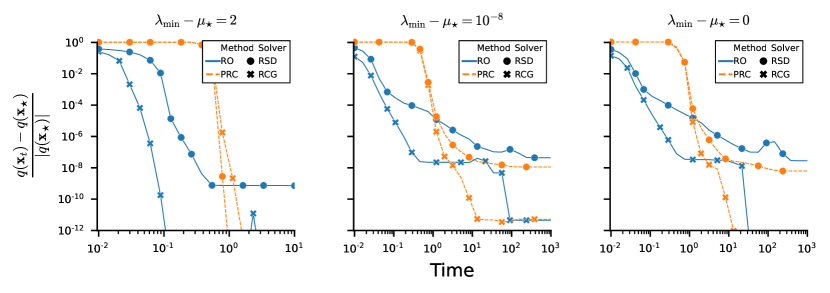
Figure 1: The progression in objective (relative) error where x axis shows the time in seconds.

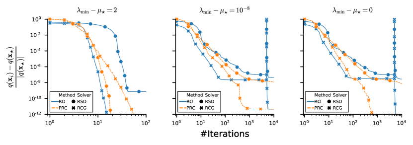
Figure 2: The progression in objective (relative) error where x axis shows the iteration number.

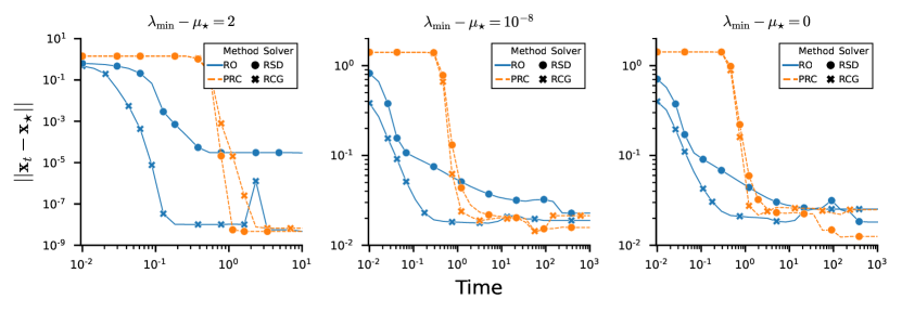
Figure 3: The progression in argument error where x axis shows the time in seconds.

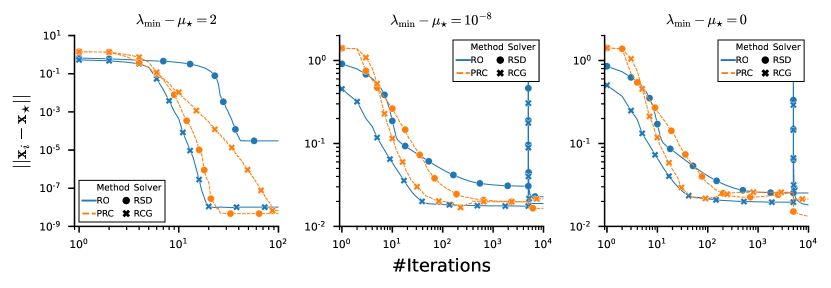
Figure 4: The progression in argument error where x axis shows the iteration number.

Appendix A Constructing $\phi$

We now show a simple way to construct a smooth $\phi(\cdot)$ fulfilling both requirements stated in Items 1 and 2 in Equation 23.

First, we choose some time parameter $\epsilon>0$ and set $d\coloneqq\lambda_{\min}({\bm{\mathrm{M}}})-\epsilon$. We construct $\phi(\alpha)$ to be a smoothed out over-estimation of $\max(\alpha,-d)$. We first construct an under estimation. Let $\gamma>1$ be another parameter, and define

$$\varphi(\alpha)=\frac{\alpha+d}{2}\left(1-\tanh\left(-\gamma\left(\alpha+d\right)\right)\right)-d.$$

Then $\varphi(\alpha)$ is a smooth function that approximates $\max(\alpha,-d)$, but it is an under estimation: $\varphi(\alpha)\leq\max(\alpha,-d)$.

While the difference between $\max(\alpha,-d)$ and $\varphi(\alpha)$ reduces significantly when $\gamma$ grows, we want to make sure that our approximation is greater than or equal to the $\max(\alpha,-d)$. To that end, let

$$\alpha_{0}\coloneqq-\frac{\operatorname{W}\left[0,e^{-1}\right]+1}{2\gamma}-d,$$

where $\operatorname{W}\left[0,\cdot\right]$ is the zero branch of the Lambert-$\operatorname{W}$ function. Now, set:

(26) $$\phi(\alpha)\coloneqq\varphi(\alpha)-\varphi(\alpha_{0})-d.$$

See Figure 5 for a graphical illustration of $\phi$. It is possible to show that

(27) $$0\leq\phi(\alpha)-\max(\alpha,-\lambda_{\min}({\bm{\mathrm{M}}}))\leq\frac{\operatorname{W}\left[0,e^{-1}\right]+1}{2\gamma}(1-\tanh((\operatorname{W}\left[0,e^{-1}\right]+1)/2)))+\epsilon,$$

so Item 1 holds, and the approximation error (Item 2) is small if $\epsilon$ is sufficiently small and $\gamma$ is sufficiently large. The proof of Equation 27 is rather technical and does not convey any additional insight on the btrs and its solution, so we omit it.

Figure 5: Illustration of the approximation’s behavior. Values of the variable $\alpha$ are depicted in the x axis. Note that $\phi(-\alpha)>-\lambda_{\min}({\bm{\mathrm{M}}})$ for all $\alpha$, while in addition $\phi(\alpha)$ well approximates $\alpha$ for values of $\alpha\geq-\lambda_{\min}({\bm{\mathrm{M}}})$.

References

- [1] P.-A. Absil, R. (Robert) Mahony, and R. (Rodolphe) Sepulchre. Optimization algorithms on matrix manifolds. Princeton University Press, 2008.
- [2] Satoru Adachi, Satoru Iwata, Yuji Nakatsukasa, and Akiko Takeda. Solving the Trust-Region Subproblem By a Generalized Eigenvalue Problem. SIAM Journal on Optimization, 27(1):269–291, 2017.
- [3] Ainesh Bakshi, Nadiia Chepurko, and R. Jayaram. Testing positive semi-definiteness via random submatrices. In 61st Annual IEEE Symposium on Foundations of Computer Science, 2020.
- [4] Amir Beck and Yakov Vaisbourd. Globally Solving the Trust Region Subproblem Using Simple First-Order Methods. SIAM Journal on Optimization, 28(3):1951–1967, 2018.
- [5] N. Boumal, V. Voroninski, and A.S. Bandeira. Deterministic guarantees for Burer-Monteiro factorizations of smooth semidefinite programs. Communications on Pure and Applied Mathematics, 73(3):581–608, 2019.
- [6] Nicolas Boumal. An introduction to optimization on smooth manifolds. To appear with Cambridge University Press, Apr 2022.
- [7] Yair Carmon and John C Duchi. Analysis of Krylov subspace solutions of regularized non-convex quadratic problems. In S. Bengio, H. Wallach, H. Larochelle, K. Grauman, N. Cesa-Bianchi, and R. Garnett, editors, Advances in Neural Information Processing Systems 31, pages 10705–10715. Curran Associates, Inc., 2018.
- [8] Ll. G. Chambers and R. Fletcher. Practical Methods of Optimization. The Mathematical Gazette, 85(504):562, 2001.
- [9] Olivier Chapelle, Vikas Sindhwani, and S. Sathiya Keerthi. Branch and bound for semi-supervised support vector machines. In Proceedings of the 19th International Conference on Neural Information Processing Systems, NIPS’06, pages 217–224, Cambridge, MA, USA, 2006. MIT Press.
- [10] Mihai Cucuringu and Hemant Tyagi. Provably robust estimation of modulo 1 samples of a smooth function with applications to phase unwrapping. arXiv e-prints, page arXiv:1803.03669, 2018.
- [11] Alan Edelman, Tomás A Arias, and Steven T Smith. The geometry of algorithms with orthogonality constraints. SIAM journal on Matrix Analysis and Applications, 20(2):303–353, 1998.
- [12] Walter Gander, Gene H. Golub, and Urs von Matt. A constrained eigenvalue problem. Linear Algebra and its Applications, 114-115:815 – 839, 1989. Special Issue Dedicated to Alan J. Hoffman.
- [13] Gene H. Golub and Urs von Matt. Quadratically constrained least squares and quadratic problems. Numerische Mathematik, 59(1):561–580, 1991.
- [14] N. Gould, S. Lucidi, M. Roma, and P. Toint. Solving the trust-region subproblem using the lanczos method. SIAM Journal on Optimization, 9(2):504–525, 1999.
- [15] William W. Hager. Minimizing a quadratic over a sphere. SIAM Journal on Optimization, 12(1):188–208, 2001.
- [16] Insu Han, Dmitry Malioutov, Haim Avron, and Jinwoo Shin. Approximating spectral sums of large-scale matrices using stochastic chebyshev approximations. SIAM Journal on Scientific Computing, 39(4):A1558–A1585, 2017.
- [17] Thorsten Joachims. Transductive learning via spectral graph partitioning. In Proceedings of the Twentieth International Conference on International Conference on Machine Learning, ICML’03, pages 290–297. AAAI Press, 2003.
- [18] Stefano Lucidi, Laura Palagi, and Massimo Roma. On Some Properties of Quadratic Programs with a Convex Quadratic Constraint. SIAM Journal on Optimization, 8(1):105–122, 1998.
- [19] David G. Luenberger. Linear and nonlinear programming. Mathematics and Computers in Simulation, 28(1):78, 1986.
- [20] José Mario Martínez. Local Minimizers of Quadratic Functions on Euclidean Balls and Spheres. SIAM Journal on Optimization, 4(1):159–176, 1994.
- [21] B. Mishra and R. Sepulchre. Riemannian preconditioning. SIAM Journal on Optimization, 26(1):635–660, 2016.
- [22] Jorge J. Moré and D. C. Sorensen. Computing a Trust Region Step. SIAM Journal on Scientific and Statistical Computing, 4(3):553–572, 1983.
- [23] Jorge Nocedal and Stephen J Wright. Numerical optimization(2nd). 2006.
- [24] Anh-Huy Phan, Masao Yamagishi, Danilo Mandic, and Andrzej Cichocki. Quadratic programming over ellipsoids with applications to constrained linear regression and tensor decomposition. Neural Computing and Applications, 32(11):7097–7120, 2020.
- [25] Boris Shustin and Haim Avron. Randomized Riemannian preconditioning for orthogonality constrained problems, 2020.
- [26] Joel A. Tropp, Alp Yurtsever, Madeleine Udell, and Volkan Cevher. Practical sketching algorithms for low-rank matrix approximation. SIAM Journal on Matrix Analysis and Applications, 38(4):1454–1485, 2017.
- [27] Bart Vandereycken and Stefan Vandewalle. A riemannian optimization approach for computing low-rank solutions of lyapunov equations. SIAM Journal on Matrix Analysis and Applications, 31(5):2553–2579, 2010.