Broad-band selection, spectroscopic identification, and physical properties of a population of extreme emission line galaxies at $3<z<3.7$

Abstract

We present the selection, spectroscopic identification, and physical properties of extreme emission line galaxies (EELGs) at $3<z<3.7$ aiming at studying physical properties of an analog population of star-forming galaxies (SFGs) at the epoch of reionization. The sample is selected based on the excess in the observed Ks broad band flux relative to the best-fit stellar continuum model flux. By applying a 0.3 mag excess as a primary criterion, we select 240 EELG candidates with intense emission lines and estimated observed-frame equivalent width (EW) of $\gtrsim 1000$ Å over the UltraVISTA-DR2 ultra-deep stripe in the COSMOS field. We then carried out a HK band follow-up spectroscopy for 23 of the candidates with Subaru/MOIRCS, and find that 19 and two of them are at $z>3$ with intense [O III] emission, and $\text{H}\alpha$ emitters at $z\simeq 2$, respectively. These spectroscopically identified EELGs at $z\simeq 3.3$ show, on average, higher specific star formation rates (sSFR) than the star-forming main sequence, low dust attenuation of $E{(\mathit{B}-\mathit{V})}\lesssim 0.1$ mag, and high $\text{[{O~{}III}]}/\text{[{O~{}II}]}$ ratios of $\gtrsim 3$. We also find that our EELGs at $z\simeq 3.3$ have higher hydrogen ionizing photon production efficiencies ($\xi_{\text{ion}}$) than the canonical value ($\simeq 10^{25.2}\,\text{$\text{erg}^{-1}\,\text{Hz}$}$), indicating that they are efficient in ionizing their surrounding interstellar medium. These physical properties suggest that they are low metallicity galaxies with higher ionization parameters and harder UV spectra than normal SFGs, which is similar to galaxies with Lyman continuum (LyC) leakage. Among our EELGs, those with the largest $\text{[{O~{}III}]}/\text{[{O~{}II}]}$ and $\text{EW}(\text{[{O~{}III}]})$ values would be the most promising candidates to search for LyC leakage.

1 Introduction

Cosmic reionization is one of the most dramatic events in the course of the evolution of the universe. Since star-forming galaxies (SFGs) at early cosmic epochs, $z\gtrsim 6$, appear to dominate the reionization process (e.g., Bouwens et al., 2015; Robertson et al., 2015; Matsuoka et al., 2018), understanding the nature, such as stellar masses ($M_{\star}$), star formation rates (SFRs), metallicities, and ionization parameters of these objects provides important clues on the ionizing sources responsible to reionize the universe as well as the early phase of the galaxy formation and evolution. These high-redshift SFGs have been selected via broad-band dropout or narrow-band excess techniques (e.g., Kashikawa et al., 2006; Bouwens et al., 2008; Ota et al., 2010; Ouchi et al., 2010, 2018; Ellis et al., 2013; Ono et al., 2018), many of which are inferred to be young ($\lesssim 100$ Myr), low-mass ($M_{\star}\lesssim 10^{8\text{--}9}M_{\odot}$), actively star-forming with a specific star formation rate ($\text{sSFR}\equiv\text{SFR}/M_{\star}$) of $\gtrsim 10$ Gyr^-1, and metal-poor ($12+\log(\text{O/H})\lesssim 8$). Due to such physical conditions, their rest-frame optical emission lines such as $\text{[{O~{}III}]}\lambda\lambda 4959,5007$ and $\text{H}\alpha$ are expected to be ubiquitously strong (e.g., Faisst et al., 2016) such that the inferred rest-frame equivalent width (EW) of $\text{H}\beta+\text{[{O~{}III}]}\lambda\lambda 4959,5007$ often exceeds $\gtrsim 1000$ Å (e.g., Smit et al., 2014, 2015; Roberts-Borsani et al., 2016; Stark et al., 2017; De Barros et al., 2019; Endsley et al., 2020). However, currently available facilities both in space and on the ground do not allow spectroscopic access to these emission lines at $z\gtrsim 4$, preventing us from rest-frame optical emission line studies of interstellar medium (ISM) properties as commonly done at $z\lesssim 4$.

Alternatively, lower-redshift analogs which are likely to have the similar characteristics to high redshift galaxies have been sought. In the local universe, these galaxies are called as green peas (GPs; Cardamone et al., 2009; Amorín et al., 2010; Izotov et al., 2011) named after their green colors due to extremely strong [O III] lines (typically rest-frame $\text{EW}\gtrsim 100$ Å and sometimes exceeds $\sim 1000$ Å). At intermediate redshifts of $1\lesssim z\lesssim 3$, the grism spectroscopic capability of HST/WFC3 enables to find so-called “Extreme Emission Line Galaxies” (EELGs), SFGs with similarly large emission line equivalent widths (e.g., Straughn et al., 2008; Atek et al., 2011; van der Wel et al., 2011; Maseda et al., 2014). These studies indeed revealed the physical properties of EELGs to be young, low-mass, low metallicity, and with high sSFR which is $\gtrsim 2\sigma$ above the average $M_{\star}$–SFR relation of SFGs at $z\simeq 2$ (e.g., Whitaker et al., 2014).

Although these previous works at $z<3$ have unveiled various properties of EELGs, a detailed spectroscopic study of them as close redshifts to the epoch of reionization (EoR) as possible is desirable since the physical conditions of the universe can be significantly different at $z\gtrsim 3$. In particular, the gas consumption timescale would become similar or longer than the mass increase timescale at $z\gtrsim 3$ due to the increased matter accretion rate, which likely causes a breakdown of a self-regulation of star formation in galaxies (e.g., Lilly et al., 2013). A steep decline ($\simeq 0.3$ dex) of the gas-phase metallicity of normal SFGs from $z\simeq 2.3$ to $z\simeq 3.3$ presumably reflects the changes in the timescales (Maiolino et al., 2008; Onodera et al., 2016; Wuyts et al., 2016, but see Sanders et al. 2020a). However, only a handful EELGs have spectroscopically confirmed rest-frame emission line strengths at $z>3$ and most of them are gravitationally lensed sources (e.g., Fosbury et al., 2003; Amorín et al., 2014; Bayliss et al., 2014; de Barros et al., 2016; Cohn et al., 2018). Therefore, a systematic study of EELGs at $z\gtrsim 3$ is still required to obtain a comprehensive picture of the population itself and to understand their higher redshift counterparts (see also Tran et al. 2020 for a recent observation of rest-frame optical emission lines of EELGs at $3<z<3.8$).

In this study, we present a systematic search of EELGs at $3\lesssim z\lesssim 3.7$ with observed-frame $\text{EW}(\text{H}\beta+\text{[{O~{}III}]}\lambda\lambda 4959,5007)>1000\,\text{\AA}$ based on photometric data, and their spectroscopic properties from our near-infrared (IR) follow-up observation. The selection method and photometric properties of the sample are presented in Section 2. Spectroscopic follow-up is presented in Section 3, and we derive physical parameters of the spectroscopically confirmed objects in Section 4. In Section 5, we show the results on the physical properties of the identified EELGs at $z\simeq 3.3$ and discuss the implications for the Lyman continuum (LyC) photon escape from these objects and for properties of galaxies in the EoR. We summarize our results in Section 6.

Throughout the paper, we adopt the WMAP 7 cosmology (Komatsu et al., 2011) with $H_{0}=70.4\,\,\text{km}~{}\text{s}^{-1}{\,}\mathrm{Mpc}^{-1}$, $\Omega_{\text{m}}=0.272$, and $\Omega_{\Lambda}=1-\Omega_{\text{m}}$, and AB magnitude system (Oke & Gunn, 1983).

2 Sample selection

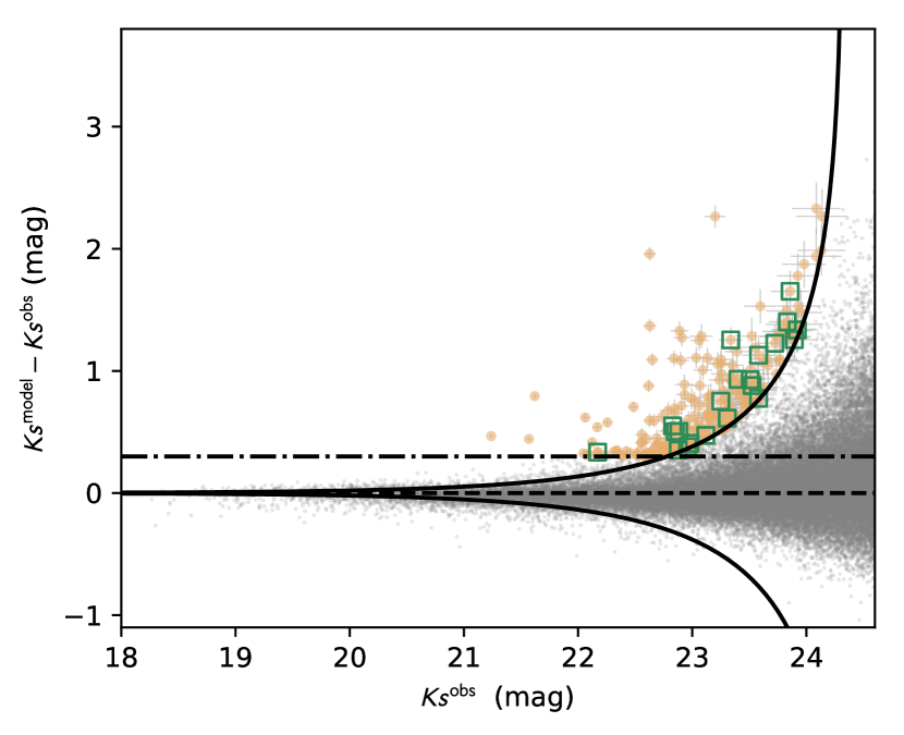
Figure 1: Color excess in Ks band, $\Delta m_{\mathit{Ks}}$, as a function of observed Ks-band magnitude for all galaxies (dots) in the ultra-deep stripes of UltraVISTA-DR2. Beige circles with error bars highlight objects selected as EELG candidates satisfying the criteria $\Delta m_{\mathit{Ks}}>0.3$ (dash-dotted line) and Equation 2 (solid lines) on the positive side. Objects with spectroscopic identification by our Subaru/MOIRCS observation are shown with squares. Dashed line indicates the case of no excess.

We use the COSMOS2015 catalog (Laigle et al., 2016) for the sample selection. The COSMOS2015 catalog contains multiband photometric data in the 2 deg² COSMOS field (Scoville et al., 2007), including Y-band Hyper Suprime-Cam (HSC) image (Tanaka et al., 2017), YJHKs UltraVISTA-DR2 images (McCracken et al., 2012), and $3.6\,\micron$ and $4.5\,\micron$ IR data from the Spitzer Large Area Survey with Hyper Suprime-Cam (SPLASH) project. The goal of our photometric selection is to construct a parent sample of objects at $3\lesssim z\lesssim 3.7$ with excess fluxes in the Ks-band due to intense $\text{H}\beta$ and $\text{[{O~{}III}]}\lambda\lambda 4959,5007$ lines.

In order to estimate the contribution from the emission lines in the Ks-band magnitude, we first estimated stellar continuum by using the best-fit model spectral energy distribution (SED) obtained by EAZY (Brammer et al., 2008). For the EAZY run, we fixed the redshifts to COSMOS2015 photometric redshifts and used $3^{\prime\prime}$ aperture magnitudes in CFHT/MegaCam u-band (Capak et al., 2007), Subaru/Suprime-Cam B-, V-, r-, ip-, and zpp-band (Taniguchi et al., 2007, 2015), VISTA/VIRCAM YJH-band (McCracken et al., 2012), and Spitzer/IRAC $3.6\,\micron$ and $4.5\,\micron$ data (Moneti et al., in preparation). We derived the stellar-only model Ks magnitude, Ks^model, by convolving the best-fit SED with the VISTA/VIRCAM Ks-band transmission. We then computed the difference between Ks^model and the observed Ks magnitudes, Ks^obs, $\Delta m_{\mathit{Ks}}\equiv\mathit{Ks}^{\mathrm{model}}-\mathit{Ks}^{\mathrm{obs}}$. The Ks-band excess magnitude is related to the observed-frame emission line equivalent widths as

$$\Delta m_{\mathit{Ks}}=-2.5\log\frac{\mathrm{FWHM}_{\mathit{Ks}}}{\mathrm{EW}_{\text{obs}}(\text{[{O~{}III}]}+\text{H}\beta)+\mathrm{FWHM}_{\mathit{Ks}}},$$ (1)

where $\text{FWHM}_{\mathit{Ks}}$ is the band width of the VISTA Ks-band filter (3090 Å; Laigle et al., 2016). Our primary selection criterion is $\Delta m_{\mathit{Ks}}>0.3$ corresponding to the observed-frame $\mathrm{EW}>1000\,\mathrm{\AA}$ (Yamada et al., 2005). At fainter magnitudes, one has to take the photometric errors into account. Following Bunker et al. (1995), we use the Ks-band magnitude-dependent criteria,

$$\Delta m_{\mathit{Ks}}=-2.5\log_{10}\left[1-\frac{\Sigma\sqrt{f_{1\sigma_{\mathrm{model}}}^{2}+f_{1\sigma_{\mathrm{obs}}}^{2}}}{f_{\mathrm{obs}}}\right]$$ (2)

where $f_{\mathrm{obs}}$, $f_{1\sigma_{\mathrm{obs}}}$, and $f_{1\sigma_{\mathrm{model}}}$ are an observed flux, $1\sigma$ error in the observed flux, and $1\sigma$ error in the model flux, respectively, and $\Sigma$ sets the significance of the flux excess. Here, we adopt $\Sigma=3$ and $f_{1\sigma_{\mathrm{obs}}}$ converted from the $3\sigma$ depth of the ultra-deep stripes of UltraVISTA-DR2, 24.7 mag, as described in Laigle et al. (2016), while we assume $f_{1\sigma_{\mathrm{model}}}=0$ for the model flux.

Figure 1 shows $\Delta m_{\mathit{Ks}}$ as a function of the observed Ks-band magnitude for all galaxies in the ultra-deep stripes. Objects satisfying $\Delta m_{\mathit{Ks}}>0.3$ and Equation 2 are shown with beige circles. There are 240 such EELG candidates in the ultra-deep stripes of which 142 of them are $3<z_{\text{phot}}<3.7$. Note that we only consider galaxies in a 0.46 deg² area of non-flagged regions both in UltraVISTA-DR2 and in the optical images (Capak et al., 2007).

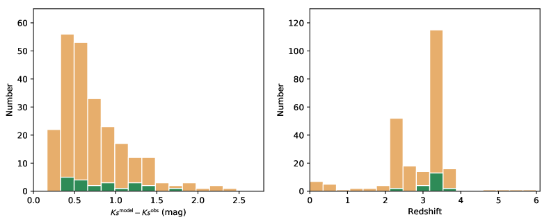
Figure 2: Histograms of $\Delta m_{\mathit{Ks}}$ (Left) and redshift (Right) of 240 EELG candidates selected in Section 2 (beige). The distributions of spectroscopically confirmed objects are overplotted with green histograms.

The left panel of Figure 2 shows the distribution of $\Delta m_{\mathit{Ks}}$ of the EELG candidates as a beige histogram. While the cut at 0.3 mag is our selection criteria, the flux excess distribution shows a long tail reaching to $\sim 2.3$ mag, corresponding to an observed EW of $\simeq 2.3\times 10^{4}\,\mathrm{\AA}$ or a rest-frame $\mathrm{EW}(\text{H}\beta+\text{[{O~{}III}]}\lambda\lambda 4959,5007)\simeq 5300\,\mathrm{\AA}$ at $z\simeq 3.3$, though part of such a large apparent excess can be due to large photometric errors at fainter $\mathit{Ks}^{\text{obs}}$. Most of the objects have $\Delta m_{\mathit{Ks}}<1.5$ corresponding to the rest-frame $\mathrm{EW}(\text{H}\beta+\text{[{O~{}III}]}\lambda\lambda 4959,5007)\lesssim 3000\,\mathrm{\AA}$. This can be translated into $\mathrm{EW}(\text{[{O~{}III}]}\lambda 5007)\lesssim 2000\,\mathrm{\AA}$ (Reddy et al., 2018a).

The redshift distribution of the EELG candidates are shown in the right panel of Figure 2. Here photometric redshifts from the COSMOS2015 catalog are adopted. EELG candidates with Ks-band excess are mostly confined at $2\lesssim z\lesssim 3.7$ with two notable peaks at $z\simeq 2.3$ and $z\simeq 3.4$, corresponding to $\text{H}\alpha$ emitters and [O III] emitters, respectively. A small number of objects (about 10 %) is found outside this confined peaks. Looking at their SEDs, the most likely explanation of these outliers is wrong photometric redshifts and sometimes large photometric uncertainties in optical bands.

We have also carried out the same selection procedure for galaxies in the deep layer of UltraVISTA-DR2 by setting the $3\sigma$ Ks-band magnitude limit as 24.0 and found 318 objects satisfying the aforementioned criteria. However, because of the shallower YJHKs images of UltraVISTA-DR2 up to 0.7 mag, photometric errors in these bands seem too large to robustly constrain the continuum flux in SED fitting and the resulting selection appears to be significantly more uncertain than that in the ultra-deep stripes. In order to keep the purity of the selection as much as possible, we restrict our analysis and subsequent follow-up spectroscopy to the objects in the ultra-deep stripes.

3 Spectroscopic follow-up observation

3.1 Follow-up near-IR spectroscopy

We carried out a spectroscopic follow-up observation for a subset of the Ks-band excess EELG candidates. Spectroscopic targets were selected primarily to maximize the number of observed EELG candidates with $3<z_{\mathrm{phot}}<3.7$. We also supplementarily considered criteria $\mathit{rJL}\equiv(\mathit{J}-[3.6])-1.4(\mathit{r}-\mathit{J})>0$ which was proposed to select objects at $2.5\lesssim z\lesssim 4$ (Daddi et al., 2004), and iJHK colors to remove low redshift ($z\lesssim 0.2$) emission line galaxies (Tadaki et al., 2013).

We used Multi-Object InfraRed Camera and Spectrograph (MOIRCS; Ichikawa et al., 2006; Suzuki et al., 2008) at the Subaru Telescope. The two detectors of MOIRCS have been replaced from Hawaii-2 to Hawaii-2RG in 2015 (Fabricius et al., 2016; Walawender et al., 2016). We used the HK500 grism covering $1.3\,\micron$ to $2.3\,\micron$ with a $0.8$ arcsec slit which provides the spectral resolution of $R\simeq 350$. After the detector upgrade, the lower readout noise allows us to shorten the exposure time to reach the background limited performance, enabling us to better capture the temporal variation of the sky background. Although the throughput in the HK-band improved only by $\lesssim 5$ %, the lower readout noise results in a deeper limiting flux than the previous detectors by cleaner sky subtraction, which is crucial for the relatively low resolution of the HK500 grism used in this study.

The observation was carried out during the first half nights on April 9 and 17, 2017 under clear sky condition with 0.5–0.8 arcsec seeing. Three masks for three pointings (each has a diameter of $\simeq 6$ arcmin) were used to observe in total 23 EELG candidates. We used a modified AB dithering pattern with three dithering widths of 2.8, 3.0, and 3.2 arcsec to increase the signal-to-noise ratio (S/N) and to avoid bad pixels (Kriek et al., 2015), and 180 s on-source exposure per dithering position. Each mask has been integrated $\simeq 40$–$110$ minutes. The detailed observing log is shown in Table 1. We observed A0V-type stars at the beginning of the nights for flux calibration as well as telluric correction using the identical instrument setup to the science exposures.

Data reduction was carried out using the MCSMDP pipeline (Yoshikawa et al., 2010) and custom scripts. Since the original MCSMDP was developed for the previous detectors, we made modifications to properly handle the new Hawaii-2RG detectors. The data were flat-fielded by using dome-flat frames which were taken under the identical instrument setup to the science frames. Bad pixels and cosmic rays were identified by using bad-pixel maps created for the new detectors and by using the pair of images in the dithering, respectively, and linearly interpolated using adjacent pixels along the spatial direction. Background sky was subtracted by taking a difference between A and B positions. The optical distortion was then corrected by applying a polynomial function determined by the MOIRCS imaging reduction pipeline MCSRED.

Individual 2-dimensional (2D) spectra were extracted from each frame and the wavelength calibration was carried out by using OH-airglow lines (Rousselot et al., 2000). The typical uncertainty of the wavelength calibration is $\simeq 3$ Å which is about 40 % of the pixel scale. Based on the wavelength solution, the extracted 2D spectra were rectified so that sky lines are aligned along the spatial direction and the secondary sky subtraction procedure was made in order to remove residual background by fitting a linear function at each wavelength pixel.

Standard star frames of A0V-type stars were processed in the same manner as the science object frames. The 1D spectra of the standard stars were extracted using the apall task in Image Reduction and Analysis Facility (IRAF; Tody, 1986, 1993) and system total response curve was derived by comparing the observed spectra with a theoretical template (Kurucz, 1979). Along with the telluric correction, we have carried out absolute flux calibration for the standard spectra by scaling them to 2MASS magnitudes correcting for the slit loss. Flux calibrated 2D frames of each object are then median stacked after $3\sigma$ clipping with offsets corresponding to the dithering widths. One dimensional noise spectra were calculated using the $1\sigma$ dispersion of the counts along the spatial direction at each wavelength pixel in the non-detected slits for each mask after the stacking procedure.

One dimensional science and corresponding noise spectra were extracted by adopting the optimal extraction algorithm (Horne, 1986). Here, we assume a Gaussian spatial profile at the strongest detected emission line for weighting and a straight trace for extraction. Before the extraction, we confirmed that the trace is straight along the dispersion direction by using bright stars and galaxies put in the science masks as filler targets.

Figure 3 and Figure 4, respectively, shows 2D and 1D spectra of emission line detected EELG candidates. Twenty-one out of 23 observed EELG candidates show detected emission lines and the origin of K-band excesses are confirmed as [O III] and $\text{H}\alpha$ at $z\simeq 3.3$ and $z\simeq 2.2$ for 19 and 2 objects, respectively.

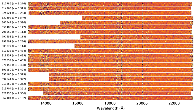
Figure 3: Two-dimensional Subaru/MOIRCS spectra of 21 EELG candidates with detected emission lines. Object IDs and spectroscopic redshifts are indicated on the left side of the spectra.

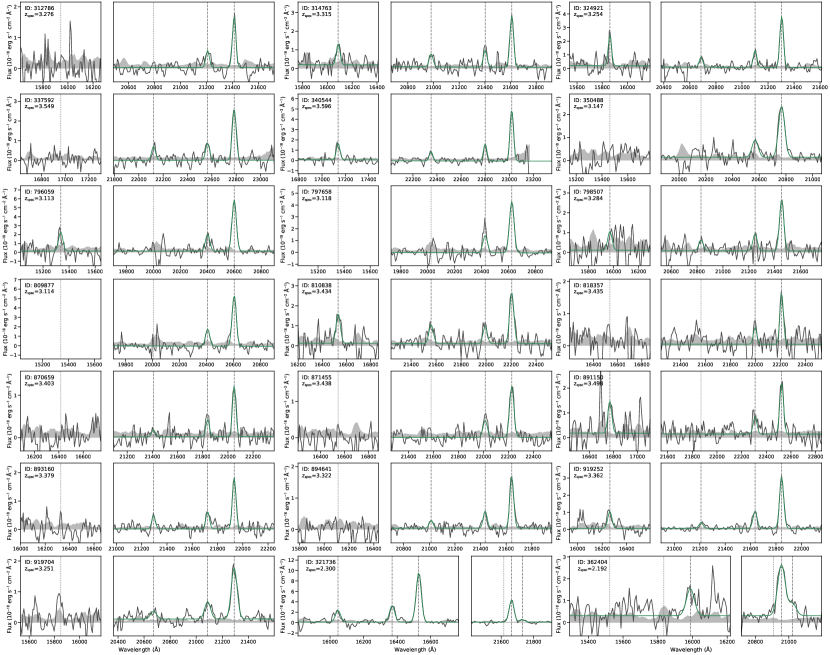
Figure 4: One-dimensional Subaru/MOIRCS spectra of 21 EELG candidates with detected emission lines. Object IDs and spectroscopic redshifts are indicated on the left side of the spectra. Spectra of each object are shown in a pair of panels corresponding to H and K bands. In each panel, object and noise spectra are shown with solid black lines and gray shaded areas, respectively, together with the best-fit Gaussian functions and continuum in green solid lines. Vertical lines show the locations of detected (dashed) and undetected (dotted) emission lines. These emission lines corresponds to $\text{[{O~{}II}]}\lambda 3727$, $\text{H}\beta$, and $\text{[{O~{}III}]}\lambda\lambda 4959,5007$ for the first 19 objects, and $\text{H}\beta$, $\text{[{O~{}III}]}\lambda\lambda 4959,5007$, $\text{[{N~{}II}]}\lambda 6548$, $\text{H}\alpha$, and $\text{[{N~{}II}]}\lambda 6583$ for the last two objects, from left to right.

Table 1: EELG candidates for the near-IR spectroscopic follow-up with Subaru/MOIRCS

ID	R.A.	Decl.	$z_{\mathrm{phot}}$	$\mathit{Ks}_{\mathrm{tot}}$	$\Delta m_{\mathit{Ks}}$	$T_{\mathrm{exp}}$
	(deg)	(deg)		(mag)	(mag)	(minutes)
(1)	(2)	(3)	(4)	(5)	(6)	(7)
312786	149.77668	1.763990	3.326	23.50	0.93	108
314763	149.74508	1.766926	3.520	22.85	0.55	108
324921	149.73393	1.782772	3.464	22.91	0.38	108
337592	149.78500	1.802777	3.555	23.87	1.65	108
340544	149.79346	1.807244	3.524	23.61	0.78	108
350488	149.77386	1.822980	3.422	23.04	0.41	108
796059	150.42306	2.509079	3.316	22.86	0.51	042
797658	150.47565	2.511852	3.320	23.59	1.13	042
798507	150.44682	2.512701	3.374	23.31	0.75	042
809877	150.46558	2.529429	3.166	23.36	1.25	042
810838	150.50135	2.531063	3.500	23.34	0.61	042
818357	150.50653	2.542366	3.402	23.99	1.26	042
870659	149.80901	2.622814	3.416	23.77	1.40	084
871455	149.79484	2.623711	3.407	23.56	0.88	084
891150	149.77483	2.653322	3.541	22.88	0.35	084
893160	149.84076	2.656873	3.316	24.00	1.34	084
894641	149.83600	2.659291	3.354	23.71	1.23	084
919252	149.82153	2.696576	3.292	23.36	0.93	084
919704	149.79926	2.697392	3.249	22.88	0.50	084
321736	149.79515	1.777986	2.300	23.13	0.47	108
362404	149.74646	1.841587	2.199	22.13	0.34	108
348570	149.76113	1.819842	3.774	23.42	0.73	108
815834	150.44337	2.538413	2.476	23.00	0.52	042

Note. — (1) Object ID (Laigle et al., 2016); (2) R.A.; (3) Decl; (4) photometric redshift from Laigle et al. (2016); (5) total Ks magnitude; (6) $\Delta m_{\mathit{Ks}}$; (7) exposure time in Subaru/MOIRCS spectroscopic observation.

3.2 Emission line measurement

As seen in Figure 3 and Figure 4, 21 objects show significant detection of multiple emission lines, which makes the emission line identification and rough redshift estimate straightforward. Then we measured the emission line properties in two fitting processes as explained below.

First, we only fit the primary emission line. The primary emission line here is the strongest emission line, i.e., $\text{[{O~{}III}]}\lambda 5007$ and $\text{H}\alpha$ for $z\simeq 3.3$ and $z\simeq 2.2$, respectively. We assume a Gaussian profile with a flat continuum. Therefore, there are four free parameters, namely, the redshift, line width $\sigma$, total line flux, and constant continuum flux. We used $\pm 500$ Å from the line center for the fitting procedure. When the primary line is $\text{H}\alpha$, adjacent $\text{[{N~{}II}]}\lambda\lambda 6548,6583$ lines are fit simultaneously as they are not fully resolved. In this case, all 3 lines are assumed to have the same redshift, $\sigma$, and continuum flux. Also, $\text{[{N~{}II}]}\lambda 6548$ flux is assumed to be one third of $\text{[{N~{}II}]}\lambda 6583$ flux.

For the fitting, we used emcee, a Python implementation of an affine invariant Markov chain Monte Carlo (MCMC) algorithm (Foreman-Mackey et al., 2013; Goodman & Weare, 2010) through lmfit (Newville et al., 2019). Priors are assumed to be top-hat in all free parameters with only minimal boundaries, namely positivity of the $\sigma$ and line flux. We used 100 walkers and 1000 steps per walker of which 200 steps were used as a burn-in process and discarded from the posterior sampling. Since the S/N ratios are typically high $\gg 10$ for the primary emission lines, the convergence is quickly achieved and all parameters for line profiles are well constrained.

In the second fitting process, we fit the rest of strong emission lines, namely, $\text{[{O~{}II}]}\lambda\lambda 3726,3729$, $\text{[{Ne~{}III}]}\lambda 3869$, $\text{H}\beta$, and $\text{[{S~{}II}]}\lambda\lambda 6717,6731$ within the observed wavelength range. For $z\simeq 2.2$ objects, $\text{[{O~{}III}]}\lambda\lambda 4959,5007$ were also fit in this process. Here, the redshift and line width $\sigma$ was fixed to those determined in the first fitting process, but allowing to be different within $\pm 0.5\sigma$ and $\pm 0.1\sigma$ from those of the primary line, respectively. We also used $\pm 500$ Å from the line centers for the fitting, but continuum was assumed to be a linear function across the spectrum. Because non-primary lines are fainter than the primary and include non-detections, we used 100 walkers with 10000 steps per walker and 2000 burn-in steps to sample the posterior distributions. These numbers are large enough to distinguish between converged and non-converged parameters.

For each parameter, the best fit parameter and the corresponding $1\sigma$ error are defined as the median and the half the interval between 16 and 84 percentiles, respectively, of the posterior distribution. To judge whether the line is detected or not, we compared the best-fit line flux with the $3\sigma$ noise computed from 1D noise spectra integrated with a Gaussian weight corresponding to the primary’s line profile. While continuum fluxes are not well constrained in general for our sample as they are barely detected as seen in Figure 3 and Figure 4, this does not affect the emission line flux measurements. Table 2 shows the measured emission line properties. Here we only list emission line fluxes used in the following discussion, though we also fit $\text{[{Ne~{}III}]}\lambda 3869$ and $\text{[{S~{}II}]}\lambda\lambda 6717,6731$ together in the second fitting process. As a reference, there are 5 out of 19 and 1 of 2 objects at $z\simeq 3.3$ and $z=2.2$ with detected $\text{[{Ne~{}III}]}\lambda 3869$ and $\text{[{S~{}II}]}\lambda 6717$ at $>3\sigma$ significance, respectively.

In the following sections, we focus on 19 spectroscopically confirmed EELGs at $3.1<z<3.6$ unless explicitly mentioned. Their positions are highlighted in Figure 1 and the distributions of $\Delta m_{\mathit{Ks}}$ and spectroscopic redshifts are shown in Figure 2. The median spectroscopic redshift of them is 3.3.

Table 2: Emission line measurements

ID	$z_{\mathrm{moircs}}$	$F(\text{[{O~{}II}]}\lambda 3727)$	$F(\text{H}\beta)$	$F(\text{[{O~{}III}]}\lambda 5007)$	$F(\text{H}\alpha)$	$F(\text{[{N~{}II}]}\lambda 6583)$
(1)	(2)	(3)	(4)	(5)	(6)	(7)
[O III] emitters
312786	$3.2758$	$<1.27$	$<0.69$	$\phantom{0}{}5.59\pm 0.27$	$\cdots$	$\cdots$
314763	$3.3148$	$4.15\pm 0.80$	$2.66\pm 0.27$	$\phantom{0}{}9.83\pm 0.42$	$\cdots$	$\cdots$
324921	$3.2539$	$7.52\pm 1.19$	$2.52\pm 0.35$	$12.81\pm 0.46$	$\cdots$	$\cdots$
337592	$3.5492$	$<1.65$	$2.84\pm 0.48$	$10.41\pm 0.42$	$\cdots$	$\cdots$
340544	$3.5965$	$6.23\pm 0.52$	$3.29\pm 0.35$	$17.95\pm 0.74$	$\cdots$	$\cdots$
350488	$3.1468$	$<2.36$	$<1.89$	$12.76\pm 0.57$	$\cdots$	$\cdots$
796059	$3.1132$	$8.57\pm 1.79$	$<6.23$	$22.75\pm 0.89$	$\cdots$	$\cdots$
797658	$3.1181$	$\cdots$	$<5.76$	$18.49\pm 0.55$	$\cdots$	$\cdots$
798507	$3.2837$	$4.10\pm 0.97$	$2.35\pm 0.51$	$10.89\pm 0.59$	$\cdots$	$\cdots$
809877	$3.1144$	$\cdots$	$<6.45$	$21.12\pm 0.73$	$\cdots$	$\cdots$
810838	$3.4338$	$6.57\pm 0.67$	$4.24\pm 0.64$	$11.06\pm 0.59$	$\cdots$	$\cdots$
818357	$3.4348$	$<1.61$	$<1.52$	$\phantom{0}{}5.53\pm 0.49$	$\cdots$	$\cdots$
870659	$3.4028$	$<1.07$	$0.59\pm 0.18$	$\phantom{0}{}4.17\pm 0.32$	$\cdots$	$\cdots$
871455	$3.4381$	$<1.15$	$<0.89$	$\phantom{0}{}6.09\pm 0.37$	$\cdots$	$\cdots$
891150	$3.4976$	$5.26\pm 0.44$	$<1.62$	$\phantom{0}{}8.01\pm 0.66$	$\cdots$	$\cdots$
893160	$3.3792$	$<1.36$	$1.67\pm 0.18$	$\phantom{0}{}6.38\pm 0.31$	$\cdots$	$\cdots$
894641	$3.3216$	$<1.99$	$0.94\pm 0.15$	$\phantom{0}{}6.20\pm 0.24$	$\cdots$	$\cdots$
919252	$3.3617$	$4.14\pm 0.54$	$1.33\pm 0.25$	$11.93\pm 0.38$	$\cdots$	$\cdots$
919704	$3.2512$	$<2.87$	$1.46\pm 0.25$	$\phantom{0}{}9.41\pm 0.32$	$\cdots$	$\cdots$
$\text{H}\alpha$ emitters
321736	$2.3002$	$\cdots$	$8.60\pm 1.16$	$36.35\pm 0.70$	$15.72\pm 0.39$	$1.69\pm 0.32$
362404	$2.1923$	$\cdots$	$<2.96$	$\phantom{0}{}7.05\pm 1.29$	$13.19\pm 0.47$	$3.07\pm 0.47$
Composite of [O III] emitters
Low-mass composite	$\cdots$	$1.70\pm 0.13$	$1.22\pm 0.06$	$\phantom{0}{}9.01\pm 0.08$	$\cdots$	$\cdots$
High-mass composite	$\cdots$	$3.16\pm 0.17$	$1.46\pm 0.09$	$\phantom{0}{}9.79\pm 0.11$	$\cdots$	$\cdots$

Note. — (1) Object ID; (2) spectroscopic redshift measured from MOIRCS spectra; (3) $\text{[{O~{}II}]}\lambda 3727$ ($\text{[{O~{}II}]}\lambda 3726+\text{[{O~{}II}]}\lambda 3729$) flux; (4) $\text{H}\beta$ flux; (5) $\text{[{O~{}III}]}\lambda 5007$ flux; (6) $\text{H}\alpha$ flux; and (7) $\text{[{N~{}II}]}\lambda 6583$ flux. All fluxes are in units of $10^{-17}\,\text{erg}\,\text{s}^{-1}\,\text{cm}^{-2}$, not corrected for dust extinction and stellar absorption. Quoted upper limits are the $3\sigma$ upper limit.

4 Measurement of physical properties

4.1 Broad-band SED fitting

We carried out a SED fitting to broad-band photometry to obtain primarily stellar masses. Subaru/HSC Y band data are also used in addition to the the photometric bands used to derive $\Delta m_{\mathit{Ks}}$. Photometry is converted to the total magnitudes from 3 arcsec aperture magnitudes following Appendix A.2 in Laigle et al. (2016). Upper limits are assigned when the fluxes are below $3\sigma$ significance.

SED fitting was performed by using the 2018.0 version of Code for Investigating GALaxy Emission (CIGALE ; Burgarella et al., 2005; Noll et al., 2009; Boquien et al., 2019). As SED templates, we used composite stellar population models generated from the simple stellar population models of Bruzual & Charlot (2003, hereafter BC03) with a Chabrier initial mass function (IMF; Chabrier, 2003) with lower and upper mass cutoffs of $0.1\,M_{\odot}$ and $100\,M_{\odot}$, respectively. Stellar population age ranges in $\log\text{age}/\text{yr}=7$–$9.6$ with steps of 0.1 dex. The upper limit of the age is assumed not to exceed the age of the universe at $z=3$. Metallicities are allowed to have $Z=0.004$, $0.008$, and $0.02$.

We consider delayed-$\tau$ models, $\text{SFR}\propto t\exp(-t/\tau)$, for the star formation history (SFH) with $\log\tau/\text{yr}=8$–$10$ with steps of 0.1 dex. Recent studies of SFH of EELGs at low and high redshifts suggest that they are in a starburst phase. Telles & Melnick (2018) studied SFH of local H II galaxies with a three-burst SFH and found that the bulk of stellar mass of them has been formed by the past star formation episode, while they are currently in a maximum starburst phase. At higher redshifts similar to our sample, Cohn et al. (2018) found that EELGs at $2.5<z<4$ show evidence of a starburst in the most recent 50 Myr with rising SFH in the last 1 Gyr. These results suggests that delayed-$\tau$ models are more representative SFH for EELGs than a constant and exponentially declining SFHs. Note that in the later analysis, we will only use the stellar mass from the SED fitting and the stellar mass is a robust parameter against the assumption of SFH.

For intense emission line galaxies like the EELGs studied here, inclusion of emission lines has critical importance (e.g., Schaerer et al., 2013; Stark et al., 2013; Onodera et al., 2016) to extract physical parameters from SED fitting. For example, changes in stellar masses can be $\gtrsim 0.5$ dex when the contribution of $\text{H}\beta+\text{[{O~{}III}]}\lambda\lambda 4959,5007$ fluxes is $\gtrsim 50$ % in the Ks band (Onodera et al., 2016). Instead of subtracting emission line contributions from broad-band photometry (Onodera et al., 2016), we include nebular emissions as supported in CIGALE. We assumed an ionization parameter of $\log U=-2.5$ which is a typical value for star-forming galaxies on the star-forming main sequence (MS) at $z\sim 3.3$ (Onodera et al., 2016). LyC photons are assumed to be entirely absorbed by neutral hydrogen, i.e., zero LyC escape fraction ($f_{\text{esc}}$) and no LyC absorption by dust. As we will discuss later, some of our EELGs at $z\simeq 3.3$ are likely to have non-zero $f_{\text{esc}}$. However, the photometric data from the COSMOS2015 catalog do not allow us to put meaningful constraints on the $f_{\text{esc}}$ with CIGALE. Indeed, the output parameters used in the following discussion are consistent well within the corresponding errors even if we set $f_{\text{esc}}$ as a free parameter. Therefore, we simply adopt the fitting results with $f_{\text{esc}}=0$. Nebular contributions (i.e., emission lines and continuum) are calculated following Inoue (2011) in CIGALE. Although the line width is not important for broad-band data, we set FWHM of emission line as 300 $\,\text{km}~{}\text{s}^{-1}$.

In CIGALE dust attenuation is implemented as a modified starburst law, $k_{\lambda}$, which is based on the Calzetti curve (Calzetti et al., 2000), $k_{\lambda}^{\text{starburst}}$, with flexibilities to add an UV bump and alter the overall slope as follows.

$$k_{\lambda}=D_{\lambda}+k^{\text{starburst}}_{\lambda}\left(\frac{\lambda}{550\,\text{nm}}\right)^{\delta}\frac{E(\mathit{B}-\mathit{V})_{\delta=0}}{E(\mathit{B}-\mathit{V})_{\delta}},$$ (3)

where $D_{\lambda}$ is the Drude profile to express an UV bump and $\delta$ modifies the slope (Noll et al., 2009). We assumed the average SMC Bar extinction curve from Gordon et al. (2003) which can be approximated by setting $D_{\lambda}=0$ and $\delta=-0.62$. The nebular extinction $E{(\mathit{B}-\mathit{V})}_{\text{neb}}$ is allowed to vary between 0 to 0.8 with steps of 0.01 in the fitting. Because nebular emission lines are explicitly taken into account in the fit, one needs to make further assumptions on the attenuation curve and the relation between attenuation affecting stellar continuum and nebular emission. Here we also used the same SMC Bar curve (Gordon et al., 2003) for nebular emission lines and assumed $E{(\mathit{B}-\mathit{V})}_{\text{neb}}=3.06\,E{(\mathit{B}-\mathit{V})}_{\text{star}}$. The latter relationship has been recently obtained by Theios et al. (2019) for the case of the SMC attenuation curve using a sample of star-forming galaxies at $2<z<2.7$ (Steidel et al., 2014; Strom et al., 2017).

At $z\gtrsim 3$, absorption by the intergalactic medium (IGM) in the observed optical bands cannot be ignored (e.g. Madau, 1995; Inoue & Iwata, 2008). When shifting the template SEDs to the observed redshift, CIGALE applies the IGM absorption using the prescription of Meiksin (2006).

The best-fit values and their corresponding standard deviations are computed based on probability distribution functions (PDFs) implemented as the pdf_analysis module (see Noll et al. 2009 and Boquien et al. 2019 for the details). The observed and best-fit SEDs are shown in Figure 5 and the resulting stellar masses, UV spectral slopes (see Section 4.2), attenuation parameters, SFRs, and stellar ages for EELGs at $z>3$ are listed in Table 3.

As seen in Figure 5, most of EELGs show a flat or power-law continuum in the optical to near-IR bands corresponding to young stellar populations with an excess flux in the K band due to the intense $\text{[{O~{}III}]}\lambda 5007$ line. There are a couple objects, namely 350488 and 919704, showing redder SEDs than the others. These two objects indeed have the best-fit age of $\gtrsim 1$ Gyr, indicating a significant contribution of old stellar populations.

It turned out that CIGALE underestimates $\text{[{O~{}III}]}\lambda 5007$ fluxes and equivalent widths of the EELG sample on average by a factor of two in our fitting run. To check this effect on the estimate of the SED properties, especially stellar masses, we ran CIGALE without Ks-band data while keeping other inputs identical, and found that stellar masses from the no-Ks run are larger than those from our fiducial run up to $0.2$ dex with a median of $0.04$ dex. The difference tends to be larger at lower stellar masses ($\log M_{\star}/M_{\odot}\lesssim 9$) with a median of $0.08$ dex. These differences are, however, smaller than the uncertainties of stellar masses and the results and discussion presented later will remain unchanged.

The underestimated best-fit predicions of [O III] fluxes and equivalent widths could be an indication of higher ionization parameters in EELGs at $z\simeq 3.3$ than $\log U=-2.5$ assumed in the CIGALE run. Although $\log U>-2.0$ seems unrealistically high for SFGs (e.g., Yeh & Matzner, 2012; Shirazi et al., 2014; Strom et al., 2018), we carried out a CIGALE run with a fixed $\log U=-1$ which is a theoretical maximum (Yeh & Matzner, 2012). It is found, however, that the predicted $\text{[{O~{}III}]}\lambda 5007$ properties are still underestimated, though the discrepancies become smaller. Therefore, the issue cannot be solved solely by the higher ionization parameter.

The lower limit of the stellar population age in the SED fitting could also limit the $\text{[{O~{}III}]}\lambda 5007$ properties. To check this possibility, we run CIGALE by adding $1$–$10$ Myr stellar populations. We found that the best-fit $\text{EW}(\text{[{O~{}III}]}\lambda 5007)$ does not always become larger by including younger stellar populations, but a clear improvement is seen for those with the highest $\text{EW}(\text{[{O~{}III}]}\lambda 5007)$ and the best-fit ages of $<10$ Myr are often derived for such cases. Similar to other CIGALE runs discussed above, there is only little change in the best-fit stellar mass ($0.01$ dex in median). Trying to find the exact match of the equivalent widths and fluxes of the $\text{[{O~{}III}]}\lambda 5007$ emission line from our EELGs sample is not a focus of this study, but it appears that higher ionization parameters and younger stellar population ages are likely to play key roles to intensify the emission line strength (see also Section 5.6; De Barros et al. 2019).

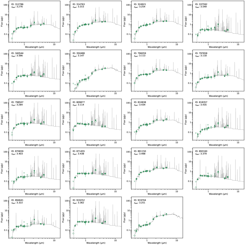
Figure 5: Broad-band SEDs of 19 spectroscopically identified EELG candidates at $z\simeq 3.3$. Filled circles and open triangles show observed fluxes and $3\sigma$ upper limits, respectively. Best-fit SED templates derived by CIGALE are shown as solid lines. Open diamonds are the best-fit SEDs convolved by the filter transmission curves used in the fit. Objects IDs and spectroscopic redshifts are shown at the upper left corner of each panel.

Table 3: Stellar mass, attenuation, star formation rate, and stellar age

ID	$\log M_{\star}$	$\beta_{\mathrm{UV,\texttt{CIGALE}}}$	$\beta_{\mathrm{UV,UV}}$	${E(\mathit{B}-\mathit{V})}_{\mathrm{star,\texttt{CIGALE}}}$	${E(\mathit{B}-\mathit{V})}_{\mathrm{star,UV}}$	$\log\mathrm{SFR}_{\mathtt{CIGALE}}$	$\log\mathrm{SFR}_{\mathrm{UV}}$	$\log\mathrm{Age}_{\mathtt{CIGALE}}$
	($M_{\odot}$)			(mag)	(mag)	($M_{\odot}{\,}\text{yr}^{-1}$)	($M_{\odot}{\,}\text{yr}^{-1}$)	(yr)
(1)	(2)	(3)	(4)	(5)	(6)	(7)	(8)	(9)
312786	$\phantom{0}{}9.58\pm 0.15$	$-1.78\pm 0.17$	$-1.84\pm 0.43$	$0.06\pm 0.02$	$0.07\pm 0.04$	$1.22\pm 0.26$	$1.24\pm 0.09$	$8.79\pm 0.27$
314763	$\phantom{0}{}9.55\pm 0.20$	$-1.17\pm 0.14$	$-1.24\pm 0.22$	$0.14\pm 0.02$	$0.12\pm 0.02$	$1.95\pm 0.25$	$1.70\pm 0.05$	$8.14\pm 0.39$
324921	$\phantom{0}{}9.83\pm 0.14$	$-1.28\pm 0.15$	$-1.41\pm 0.25$	$0.11\pm 0.02$	$0.11\pm 0.02$	$1.66\pm 0.18$	$1.60\pm 0.06$	$8.60\pm 0.27$
337592	$\phantom{0}{}8.29\pm 0.19$	$-2.13\pm 0.13$	$-2.16\pm 0.54$	$0.05\pm 0.02$	$0.04\pm 0.05$	$1.41\pm 0.15$	$0.96\pm 0.12$	$7.34\pm 0.64$
340544	$\phantom{0}{}8.95\pm 0.31$	$-1.89\pm 0.13$	$-1.77\pm 0.33$	$0.07\pm 0.02$	$0.07\pm 0.03$	$1.74\pm 0.22$	$1.38\pm 0.07$	$7.88\pm 0.72$
350488	$10.36\pm 0.08$	$-0.20\pm 0.37$	$-1.16\pm 0.73$	$0.18\pm 0.05$	$0.13\pm 0.06$	$1.23\pm 0.24$	$1.10\pm 0.16$	$9.12\pm 0.16$
796059	$\phantom{0}{}9.99\pm 0.10$	$-1.64\pm 0.13$	$-1.89\pm 0.26$	$0.07\pm 0.02$	$0.06\pm 0.02$	$1.36\pm 0.10$	$1.39\pm 0.06$	$8.97\pm 0.20$
797658	$\phantom{0}{}9.02\pm 0.24$	$-1.46\pm 0.19$	$-1.56\pm 0.51$	$0.11\pm 0.03$	$0.09\pm 0.05$	$1.47\pm 0.31$	$1.17\pm 0.11$	$8.20\pm 0.52$
798507	$\phantom{0}{}8.88\pm 0.14$	$-1.71\pm 0.10$	$-1.58\pm 0.25$	$0.10\pm 0.01$	$0.09\pm 0.02$	$1.90\pm 0.15$	$1.53\pm 0.06$	$7.43\pm 0.43$
809877	$\phantom{0}{}8.46\pm 0.07$	$-2.26\pm 0.07$	$-2.31\pm 0.27$	$0.04\pm 0.01$	$0.03\pm 0.02$	$1.66\pm 0.09$	$1.19\pm 0.06$	$7.15\pm 0.24$
810838	$\phantom{0}{}9.91\pm 0.13$	$-1.37\pm 0.18$	$-1.52\pm 0.35$	$0.10\pm 0.02$	$0.10\pm 0.03$	$1.45\pm 0.16$	$1.46\pm 0.08$	$8.84\pm 0.23$
818357	$\phantom{0}{}8.75\pm 0.32$	$-1.30\pm 0.26$	$-1.40\pm 0.85$	$0.13\pm 0.03$	$0.11\pm 0.08$	$1.56\pm 0.25$	$1.07\pm 0.19$	$7.98\pm 0.87$
870659	$\phantom{0}{}8.53\pm 0.25$	$-1.66\pm 0.17$	$-2.01\pm 0.76$	$0.10\pm 0.02$	$0.05\pm 0.07$	$1.54\pm 0.19$	$0.94\pm 0.16$	$7.61\pm 0.92$
871455	$\phantom{0}{}8.87\pm 0.26$	$-2.14\pm 0.11$	$-2.06\pm 0.30$	$0.05\pm 0.02$	$0.05\pm 0.03$	$1.55\pm 0.21$	$1.27\pm 0.07$	$7.91\pm 0.54$
891150	$\phantom{0}{}9.82\pm 0.16$	$-1.39\pm 0.14$	$-1.34\pm 0.21$	$0.10\pm 0.02$	$0.11\pm 0.02$	$1.79\pm 0.18$	$1.77\pm 0.05$	$8.48\pm 0.29$
893160	$\phantom{0}{}8.30\pm 0.17$	$-2.27\pm 0.10$	$-2.16\pm 0.48$	$0.04\pm 0.01$	$0.04\pm 0.04$	$1.32\pm 0.16$	$1.00\pm 0.10$	$7.45\pm 0.49$
894641	$\phantom{0}{}9.03\pm 0.27$	$-1.86\pm 0.23$	$-1.24\pm 0.76$	$0.06\pm 0.03$	$0.12\pm 0.07$	$1.20\pm 0.39$	$1.23\pm 0.16$	$8.55\pm 0.46$
919252	$\phantom{0}{}8.72\pm 0.15$	$-2.06\pm 0.10$	$-2.17\pm 0.27$	$0.06\pm 0.01$	$0.04\pm 0.02$	$1.75\pm 0.15$	$1.30\pm 0.06$	$7.42\pm 0.46$
919704	$10.57\pm 0.06$	$-1.39\pm 0.18$	$-1.03\pm 0.57$	$0.04\pm 0.03$	$0.14\pm 0.05$	$0.79\pm 0.21$	$1.32\pm 0.13$	$9.16\pm 0.11$
Low-mass composite	$\phantom{0}{}8.74\pm 0.33$	$-1.89\pm 0.37$	$-2.01\pm 0.35$	$0.06\pm 0.03$	$0.05\pm 0.03$	$1.55\pm 0.21$	$1.19\pm 0.18$	$7.61\pm 0.42$
High-mass composite	$\phantom{0}{}9.87\pm 0.31$	$-1.38\pm 0.23$	$-1.37\pm 0.27$	$0.10\pm 0.05$	$0.11\pm 0.02$	$1.40\pm 0.32$	$1.42\pm 0.27$	$8.82\pm 0.31$

Note. — (1) Object ID; (2) stellar mass from SED fitting; (3) UV $\beta$ slope from the best-fit SED; (4) UV $\beta$ slope from broad-band photometry; (5) $E(\mathit{B}-\mathit{V})$ for stellar continuum from SED fitting; (6) $E(\mathit{B}-\mathit{V})$ for stellar continuum from UV $\beta$ slope; (7) SFR from the best-fit SED; (8) attenuation corrected SFR based on UV luminosity; and (9) stellar population age from the best-fit SED.

4.2 UV-based dust attenuation and star formation rate

Measurements of the amount of dust attenuation and SFR are carried out by using UV part of SED, namely the UV spectral slope $\beta_{\text{UV}}$ defined as $f_{\lambda}\propto\lambda^{\beta_{\text{UV}}}$ and attenuation corrected far-UV (FUV) luminosity, respectively. We derived $\beta_{\text{UV}}$ with the identical way as Onodera et al. (2016). Briefly, we fit the total broad-band photometry in $r$, $ip$, $zpp$, $Y$, and $J$ bands with a linear function in the magnitude–$\log\lambda$ space to obtain far-UV (FUV; $\lambda\simeq 1530$Å) and near-UV (NUV; $\lambda\simeq 2300$Å) magnitudes to compute $\beta_{\text{UV}}$ following the prescription presented by Pannella et al. (2015). In the fitting, we put an additional weight of $1+\left|\lambda-\lambda_{\text{FUV}}\right|/\lambda_{\text{FUV}}$ in order to give more weights to filters closer to the rest-frame far-UV band (Nordon et al., 2013). This procedure was repeated 5000 times by artificially perturbing the photometry with the corresponding errors. The median values and standard deviations based on median absolute deviation ($\sigma_{\text{MAD}}$) of the resulting $\beta_{\text{UV}}$ and rest-frame FUV magnitude distributions are considered as the values and associated $1\sigma$ errors, respectively.

The $\beta_{\text{UV}}$ was then transformed into $E{(\mathit{B}-\mathit{V})}_{\text{star}}$ by using a recent calibration by Reddy et al. (2018b) for the SMC extinction curve (Gordon et al., 2003),

$$\beta_{\text{UV}}=-2.616+11.259\,E{(\mathit{B}-\mathit{V})}_{\text{star}}.$$ (4)

The intrinsic slope of $\beta_{\text{UV}}=-2.616$ is derived by assuming a simple stellar population of the Binary Population and Spectral Synthesis (BPASS) models (Eldridge et al., 2017) with a constant star formation with an age of 100 Myr and metallicity of $Z=0.002$, with a two-power-law IMF with $\alpha=2.35$ for $M_{\star}>0.5\,M_{\odot}$ and $\alpha=1.30$ for $0.1<M_{\star}/M_{\odot}<0.5$. The adopted relationship in Equation 4 provides $E{(\mathit{B}-\mathit{V})}_{\text{star}}$ closer to that of the original calibration by Calzetti et al. (2000) with discrepancies within $\simeq 0.1$ mag, while using the relations derived by the same authors (Reddy et al., 2015) for the Calzetti et al. (2000) and Reddy et al. (2015) attenuation curves provides systematically higher $E{(\mathit{B}-\mathit{V})}_{\text{star}}$ than that from the SMC curve by $0.03$–$0.2$ mag.

By using the derived $E{(\mathit{B}-\mathit{V})}_{\text{star}}$, SFRs were computed from attenuation corrected rest-frame FUV (1500 Å) luminosities ($L_{1500}$) using the calibration by Theios et al. (2019),

$$\log\mathrm{SFR}/(M_{\odot}{\,}\text{yr}^{-1})=\log\nu L_{\nu}(1500\,\text{\AA})/(\text{erg}\,\text{s}^{-1})-43.46.$$ (5)

This relation assumes the same intrinsic stellar population model as used to derive $E{(\mathit{B}-\mathit{V})}_{\text{star}}$ from $\beta_{\text{UV}}$, and is slightly different from that of Kennicutt & Evans (2012) where the constant term is 43.35.

The attenuation properties and SFRs derived here are shown in Table 3. These properties are compared with those derived from SED fitting in Figure 6. Both estimates agree well for $\beta_{\text{UV}}$, $E{(\mathit{B}-\mathit{V})}_{\text{star}}$, and $L_{\nu}(1500\,\mathrm{\AA}{})$ with a few outliers which are caused mainly due to large uncertainties in the rest-frame UV photometric data. SFRs derived by CIGALE SED fitting is systematically higher than those based on UV luminosities with a median difference of $0.28$ dex. The systematic difference is likely due to different assumptions in the intrinsic SED and dust attenuation. In the SED fitting, we used Bruzual & Charlot (2003) models, while BPASS models (Eldridge et al., 2017) are used in the calibration by Reddy et al. (2018b) in the UV-based estimate. Moreover, the relation between $E{(\mathit{B}-\mathit{V})}_{\text{star}}$ and $E{(\mathit{B}-\mathit{V})}_{\text{neb}}$ applied for the CIGALE run is derived assuming BPASS models and a revised version of SMC extinction curve (Reddy et al., 2016a; Theios et al., 2019). Reconciling the two estimates is not the scope of this paper, and we will use only stellar masses from the SED fitting and use UV-based estimates for the attenuation and SFR parameters in the following analysis.

Figure 6: Comparison of UV SED properties and SFR derived based on observed UV photometry (horizontal axes) and on SED fitting using CIGALE (vertical axes). (a) UV $\beta$ slope; (b) stellar $E(\mathit{B}-\mathit{V})$ assuming SMC extinction curve; (c) UV luminosity at rest-frame 1500 Å without extinction correction; and (d) extinction-corrected SFR.

4.3 Equivalent width of the $\text{[{O~{}III}]}\lambda 5007$ emission line

Table 4: Ionization properties

ID	$\text{EW}(\text{[{O~{}III}]}\lambda 5007)$	$O_{32}$	$R_{23}$	$\log\xi_{\text{ion,0}}$
	(Å)			($\mathrm{erg}^{-1}\,\mathrm{Hz}$)
(1)	(2)	(3)	(4)	(5)
312786	$\phantom{0}{}223\pm 11$	$>4.5$	$>10.5$	$<25.0$
314763	$\phantom{0}{}217\pm\phantom{0}{}9$	$1.9\pm 0.7$	$\phantom{0}{}6.5\pm 1.7$	$25.30\pm 0.07$
324921	$\phantom{0}{}250\pm\phantom{0}{}9$	$1.5\pm 0.6$	$\phantom{0}{}9.6\pm 2.8$	$25.33\pm 0.08$
337592	$2051\pm 82$	$>7.2$	$\phantom{0}{}4.8\pm 3.1$	$25.86\pm 0.15$
340544	$1391\pm 57$	$2.9\pm 1.3$	$\phantom{0}{}9.4\pm 3.4$	$25.63\pm 0.09$
350488	$\phantom{0}{}233\pm 11$	$>4.3$	$>8.5$	$<25.7$
796059	$\phantom{0}{}407\pm 16$	$2.7\pm 1.2$	$>6.5$	$<25.7$
797658	$1123\pm 33$	$\cdots$	$\cdots$	$<26.0$
798507	$\phantom{0}{}557\pm 30$	$2.5\pm 1.0$	$\phantom{0}{}8.1\pm 2.8$	$25.30\pm 0.11$
809877	$1853\pm 64$	$\cdots$	$\cdots$	$<25.8$
810838	$\phantom{0}{}262\pm 14$	$1.5\pm 0.7$	$\phantom{0}{}5.2\pm 2.0$	$25.70\pm 0.11$
818357	$\phantom{0}{}670\pm 60$	$>3.0$	$>4.6$	$<25.7$
870659	$\phantom{0}{}570\pm 43$	$>4.2$	$\phantom{0}{}8.8\pm 8.1$	$25.21\pm 0.23$
871455	$\phantom{0}{}472\pm 29$	$>5.8$	$>9.0$	$<25.0$
891150	$\phantom{0}{}153\pm 13$	$1.3\pm 0.4$	$>11.2$	$<25.0$
893160	$1171\pm 58$	$>5.3$	$\phantom{0}{}5.0\pm 2.8$	$25.54\pm 0.13$
894641	$\phantom{0}{}572\pm 22$	$>2.6$	$\phantom{0}{}7.7\pm 6.8$	$25.32\pm 0.20$
919252	$\phantom{0}{}860\pm 27$	$3.3\pm 1.3$	$14.7\pm 5.0$	$25.15\pm 0.10$
919704	$\phantom{0}{}133\pm\phantom{0}{}5$	$>2.5$	$\phantom{0}{}5.7\pm 3.8$	$25.58\pm 0.16$
Low-mass composite	$\phantom{0}{}791\pm 360$	$5.7\pm 2.5$	$10.8\pm 3.7$	$25.32\pm 0.18$
High-mass composite	$\phantom{0}{}189\pm\phantom{0}{}30$	$2.7\pm 0.5$	$\phantom{0}{}9.6\pm 1.5$	$25.43\pm 0.27$

Note. — (1) Object ID; (2) rest-frame equivalent width of $\text{[{O~{}III}]}\lambda 5007$; (3) $O_{32}$ as defined in Equation 8; (4) $R_{23}$ as defined in Equation 7; and (5) $\xi_{\text{ion,0}}$ defined in Equation 9 assuming $f_{\text{esc}}=0$.

Because our EELG sample does not show continuum in the MOIRCS spectra in general (Figure 3), emission line equivalent widths cannot be measured directly on the spectra. Furthermore, since Ks broad-band fluxes are dominated by $\text{[{O~{}III}]}+\text{H}\beta$ up to $\simeq 100$ %, estimated continuum levels based on the Ks-band photometry can be comparable to the photometric error. Therefore, we use the best-fit stellar SED derived in Section 4.1 assuming no error in the continuum. The model continuum is derived as the median flux at $4940$–$5028$ Å in the rest-frame wavelength. The derived $\text{EW}(\text{[{O~{}III}]}\lambda 5007)$ is shown in Table 4. It should be noted that the assumption of the error-free continuum is fairly strong. If we assume the same errors as the total Ks-band fluxes for the continuum, the resulting uncertainties of $\text{EW}(\text{[{O~{}III}]}\lambda 5007)$ increase from $\simeq 0.01$–$0.02$ dex to $\simeq 0.04$ dex, which does not change any of our results and conclusions presented in this study.

In Figure 7, we compare $\text{EW}(\text{[{O~{}III}]}\lambda 5007)$ with $\text{EW}(\text{[{O~{}III}]}+\text{H}\beta)$ estimated from $\Delta m_{\mathit{Ks}}$ and that predicted with a conversion derived by Reddy et al. (2018a) for a sample of star-forming galaxies at $z\simeq 3.4$. The former is derived by using Equation 1, while the latter is estimated as

$$\text{EW}(\text{[{O~{}III}]}+\text{H}\beta)=c\,\text{EW}(\text{[{O~{}III}]}).$$ (6)

The correction factor $c$ is defined as $c=0.581-0.0074x+6.322\times 10^{-3}x^{2}$ where $x=\log M_{\star}/M_{\odot}$ (Reddy et al., 2018a). Although about a half of our sample has lower stellar mass than the range of $9.0<\log M/M_{\odot}<11.5$ for which the conversion is derived, difference between two estimates agrees well with a median of 0.06 dex and a standard deviation of 0.13 dex which is smaller than the $\simeq 0.2$–$0.3$ dex scatter of the sample distribution presented in Reddy et al. (2018a).

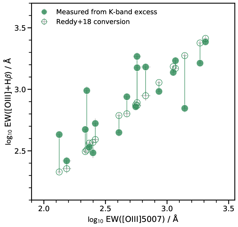
Figure 7: Comparison of $\text{EW}(\text{[{O~{}III}]}\lambda\lambda 4959,5007+\text{H}\beta)$ derived with two different methods with the spectroscopically measured $\text{EW}(\text{[{O~{}III}]}\lambda 5007)$. Filled circles show $\text{EW}(\text{[{O~{}III}]}\lambda\lambda 4959,5007+\text{H}\beta)$ derived from the Ks-band photometric excess, $\Delta m_{\mathit{Ks}}$, while open circles are predictions using a correction factor derived by Reddy et al. (2018a). Vertical lines connect each object.

4.4 $R_{23}$ and $O_{32}$ line ratios

We derived $R_{23}$ and $O_{32}$ indices defined as

$$R_{23}\equiv\frac{\text{[{O~{}II}]}\lambda 3727+\text{[{O~{}III}]}\lambda\lambda 4959,5007}{\text{H}\beta}$$ (7)

and

$$O_{32}\equiv\frac{\text{[{O~{}III}]}\lambda\lambda 4959,5007}{\text{[{O~{}II}]}\lambda 3727},$$ (8)

respectively. All emission line fluxes are corrected for dust extinction using $\beta_{\text{UV}}$-based $E{(\mathit{B}-\mathit{V})}_{\text{neb}}$ (see Section 4.2) with a conversion $E{(\mathit{B}-\mathit{V})}_{\text{neb}}=3.06\,E{(\mathit{B}-\mathit{V})}_{\text{star}}$ for the average SMC Bar extinction curve (Gordon et al., 2003; Theios et al., 2019).

We assumed $\text{[{O~{}III}]}\lambda 5007/\text{[{O~{}III}]}\lambda 4959=3$ to estimate the total [O III] flux. When $\text{[{O~{}II}]}\lambda 3727$ emission lines are not detected, we assign fluxes corresponding to the $3\sigma$ upper limit to derive the lower limit of $O_{32}$, while undetected $\text{[{O~{}II}]}\lambda 3727$ fluxes are assumed to be zero for $R_{23}$ because they are essentially negligible compared to those of $\text{[{O~{}III}]}\lambda 5007$. These upper limits are also corrected for dust extinction as described above.

Detected $\text{H}\beta$ fluxes are also corrected for stellar absorption by using the best-fit SED derived in Section 4.1. The correction factors are $\lesssim 10$ % for less massive galaxies with $\log M_{\star}/M_{\odot}<10$, while one object with $\log M_{\star}/M_{\odot}\simeq 10.5$ has a correction factor of $\simeq 40$ %. The latter value is slightly larger than the prediction using the correction factor–stellar mass relation derived by Zahid et al. (2014) for a sample of star-forming galaxies at $z\simeq 1.6$.

The derived $O_{32}$ and $R_{23}$ values are listed in Table 4.

4.5 Ionizing photon production efficiency $\xi_{\text{ion}}$

The LyC photon production efficiency, $\xi_{\text{ion}}$, is defined as the ratio of the production rate of LyC photons, $N(\mathrm{H}^{0})$ to the attenuation-corrected UV continuum luminosity density, $L_{\mathrm{UV,corr}}$:

$$\xi_{\text{ion}}=\frac{N(\mathrm{H}^{0})}{L_{\mathrm{UV,corr}}}\,\left[\mathrm{s}^{-1}/(\mathrm{erg}\,\mathrm{s}^{-1}\,\mathrm{Hz}^{-1})\right].$$ (9)

The UV luminosity is derived at the rest-frame 1500 Å using broad-band photometry (Section 4.2). For $N(\mathrm{H}^{0})$, we adopt the relation to the intrinsic $\text{H}\alpha$ luminosity, $L(\text{H}\alpha)$, by Leitherer & Heckman (1995),

$$L(\text{H}\alpha)\,\left[\mathrm{erg}\,\mathrm{s}^{-1}\right]=1.36\times 10^{-12}\,N(\mathrm{H}^{0})\,\left[\mathrm{s}^{-1}\right].$$ (10)

Then we assume $L(\text{H}\alpha)/L(\text{H}\beta)=2.86$ assuming the case B recombination with the electron density of 100 $\mathrm{cm}^{-3}$ and temperature of $10^{4}\,\mathrm{K}$ (Osterbrock & Ferland, 2006) to compute $\xi_{\text{ion}}$ for our EELG sample at $z\simeq 3.3$. The $\text{H}\beta$ fluxes are corrected for dust attenuation and stellar absorption as described in Section 4.4. One should keep in mind that the relation above is derived for an ionization-bounded H II region with no LyC escape.

LyC escape fraction is suggested to be correlated with some of galaxy properties such as $\mathit{O}_{32}$ (e.g., Nakajima & Ouchi, 2014; Nakajima et al., 2020; Faisst, 2016; Izotov et al., 2018a), $E{(\mathit{B}-\mathit{V})}$ (e.g., Reddy et al., 2016b), and $\text{Ly}\alpha$ profile (e.g., Dijkstra et al., 2016; Verhamme et al., 2015; Izotov et al., 2020). Although we have measurements of $\mathit{O}_{32}$ and $E{(\mathit{B}-\mathit{V})}$ in hand, we do not correct $f_{\text{esc}}$ here, because the correlations between $f_{\text{esc}}$ and these parameters show large scatters especially at large $\mathit{O}_{32}$ and low $E{(\mathit{B}-\mathit{V})}$ (e.g., Faisst, 2016; Reddy et al., 2016b; Nakajima et al., 2020). Instead, we use $\xi_{\text{ion,0}}$ for the case of zero LyC escape fraction (Bouwens et al., 2016; Nakajima et al., 2016) to explicitly indicate the assumption of no LyC escape from the H II region in Equation 10. The intrinsic $\xi_{\text{ion}}$ then can be derived by $\xi_{\text{ion}}=\xi_{\text{ion,0}}/(1-f_{\text{esc}})$. We will investigate the relationship between $\xi_{\text{ion,0}}$ and other galaxy properties in Section 5.4.3. The derived $\xi_{\text{ion,0}}$ are shown in Table 4.

4.6 Composite spectra

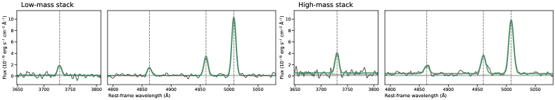
Figure 8: Stacked spectra of our EELGs at $z\simeq 3.3$ for low-mass ($\log M_{\star}/M_{\odot}\lesssim 9$) bin (two leftmost panels) and high-mass ($\log M_{\star}/M_{\odot}\gtrsim 9.5$) bin (two rightmost panels). Contents of each panel are the same as those in Figure 4 except that the horizontal axis shows the rest-frame wavelength.

In order to investigate average spectroscopic properties of EELGs at $z\simeq 3.3$, we create composite Subaru/MOIRCS spectra. We split the sample in the stellar mass at $\log M_{\star}/M_{\odot}\simeq 9.2$. There are 11 and 8 objects in the low-mass and high-mass bins, respectively. Before the stacking, each 1D spectrum is shifted and linearly interpolated to the rest-frame wavelength grid of 1 Å interval, while the corresponding noise spectrum is interpolated to the same wavelength grid in quadrature. Then composite spectra are constructed by taking an average at each wavelength weighted by the inverse variance. The associated noise spectra are derived by the standard error propagation from the individual noise spectra. Emission line fluxes are measured by fitting Gaussian components for emission lines and linear continuum similar to that applied to individual objects (Section 3.2). The resulting stacked spectra are shown in Figure 8 and emission line fluxes are shown in Table 2.

SED properties for the composite spectra are derived by taking the median and $\sigma_{\text{MAD}}$ of the sample in each bin. Equivalent widths of $\text{[{O~{}III}]}\lambda 5007$, emission line ratios, and $\xi_{\text{ion,0}}$ of the composite spectra are derived by using the derived SED properties as described above and emission line fluxes measured on the composite spectra. These parameters are appended in Table 3 and Table 4.

5 Results and discussion

5.1 Testing COSMOS2015 photometric redshifts and SED fitting

The COSMOS2015 catalog provides photometric redshifts with a precision of $\sigma_{\Delta{z/(1+z)}}=0.021$ with a catastrophic failure of $13.2$ % for star-forming galaxies at $z>3$ (Laigle et al., 2016). Although nebular emission line contributions of $\text{Ly}\alpha$, $\text{[{O~{}II}]}\lambda 3727$, $\text{H}\beta$, $\text{[{O~{}III}]}\lambda\lambda 4959,5007$, and $\text{H}\alpha$ have already taken into account when deriving the photometric redshifts, their emission line ratios are fixed to representative values for normal star-forming galaxies. For example, while they fixed $O_{32}=0.36$, our EELG sample at $z\simeq 3.3$ shows a significantly higher $O_{32}$ with the median of $\gtrsim 3$. Therefore, it is worth checking whether the photometric redshift and physical parameters in the COSMOS2015 catalog work for our EELG sample or not.

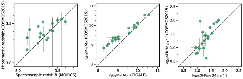
Figure 9: Comparison of photometric redshift (left), stellar mass (middle), and star formation rate (right) between the publicly available COSMOS2015 catalog (Laigle et al., 2016) and this study. Dashed lines indicate 1-to-1 relation for each parameter. Only EELGs at $3<z<3.7$ in our sample are shown.

In the left panel of Figure 9, we compare the COSMOS2015 photometric redshifts with spectroscopic ones for our identified EELG sample at $z>3$. Using the same metric as Laigle et al. (2016), we compute $\sigma_{\Delta_{z/(1+z)}}=0.025$ with a systematic offset of $-0.01$ and no catastrophic failure. Two of our spectroscopic sample are at $z_{\text{phot}}\simeq 2.2$ and their spectroscopic redshifts show almost the exact agreement. There are two objects without emission line detections. Since their COSMOS2015 photometric redshifts are 2.476 and 3.774, respectively, the primary emission lines ($\text{H}\alpha$ and $\text{[{O~{}III}]}\lambda 5007$, respectively) may fall outside of the spectral coverage of MOIRCS. Here, we conclude that the photometric redshift in COSMOS2015 for extreme emission line galaxies at $z\simeq 3.3$ is as precise as those for other galaxies at the similar redshift despite the fact that the emission line ratios assumed in the COSMOS2015 catalog is significantly different from our sample. Note, however, that the spectroscopic follow-up was carried out for a sample with visually reliable SED shapes and no attempt was done to search for EELGs at $z\simeq 3.3$ with $z_{\text{phot}}\lesssim 2$ and $z_{\text{phot}}\gtrsim 4$.

Stellar masses are compared in the middle panel of Figure 9. COSMOS2015 stellar masses are systematically larger than those derived by our SED fitting, especially evident at lower stellar masses of $\log M_{\star}/M_{\odot}\lesssim 9$. We do not find any indications that the difference between two stellar mass estimates correlates with overestimates of photo-z. Rather, this can be understood by a realistic treatment of the emission line strengths and ratios especially of [O III] to the Ks band fluxes in CIGALE using the recipe of Inoue (2011) compared to empirical line ratios in the COSMOS2015 SED fitting. Therefore, in order to estimate more appropriate stellar masses, one may not be able to rely on the catalog values for low-mass ($\log M_{\star,\mathrm{COSMOS2015}}/M_{\odot}\lesssim 9.5$) galaxies at $z\gtrsim 3$ and needs to perform a dedicated SED fitting depending on the sub-population of interest.

On the other hand, SFRs between UV-based and COSMOS2015 estimates agree well. At high SFR of $\log\text{SFR}\gtrsim 1.5$, our UV-based SFRs seems to be slightly smaller than those in the COSMOS2015 catalog. As shown in Figure 6, UV-based SFRs tend to be lower than those derived in the CIGALE SED fitting. Therefore, if $\text{SFR}_{\text{UV}}$ is replaced to $\text{SFR}_{\text{{CIGALE}}}$ in Figure 9, points will move toward right and $\text{SFR}_{\text{{CIGALE}}}$ would be higher than $\text{SFR}_{\mathrm{COSMOS2015}}$ by $\simeq 0.3$ dex.

Note also that the SED fitting in the COSMOS2015 catalog and this study use different assumptions on the set of intrinsic SED templates, dust attenuation recipes, and the explored ranges of age, metallicity, dust attenuation, and ionization parameters, which could introduce systematics for the estimate of physical parameters.

5.2 AGN contamination

Intense [O III] emission with a large EW and large $\text{[{O~{}III}]}/\text{H}\beta$ ratio can originate from AGN as well as star-forming galaxies (e.g. Baskin & Laor, 2005; Kewley et al., 2006; Caccianiga & Severgnini, 2011). Since our primary motivation in this study is to search for a population of EELGs at $z\gtrsim 3$ as an analog of star-forming galaxies in the EoR, we would like to check whether AGN dominate the sample or not.

Among 240 objects in the parent sample, 142 objects have $3<z_{\text{phot}}<3.7$ and none of them show counterparts in X-ray in the Chandra COSMOS Legacy Survey catalog (Civano et al., 2016; Marchesi et al., 2016) and in radio in the public VLA data.

There are 4 EELG candidates showing Spitzer/MIPS $24\,\mu\text{m}$ detections ranging from 70–240 $\mu\text{Jy}$. The $24\,\micron$ fluxes roughly correspond to $\text{SFR}\gtrsim 1000\,M_{\odot}{\,}\text{yr}^{-1}$ using the Dale & Helou (2002) templates to convert $24\,\micron$ fluxes to total IR luminosities and the Kennicutt (1998) relation to convert total IR luminosities to SFRs (e.g., Wuyts et al., 2008; Marchesini et al., 2010). If the $24\,\micron$ fluxes are due to star formation, they are well above the MS at $z\simeq 3.3$ (e.g., Speagle et al., 2014) and they would be detected in far-IR to submillimeter wavelength. However, none of 140 EELG candidates at $3<z_{\text{phot}}<3.7$ are detected in 100–500 µm in the Herschel/PACS PEP survey (Lutz et al., 2011) and Herschel/SPIRE HerMes survey (Oliver et al., 2012). Therefore, these MIPS $24\,\micron$ sources can be hosts of obscured AGN, but they are a rare among the selected EELG candidates, only $\lesssim 5$ %. Although the discussion above does not rule out the presence of low-luminosity or less obscured AGN undetected in $24\,\micron$, based on the available information for emission line properties, it is unlikely that AGN dominate the EELG population at $z\simeq 3.3$ as we discuss below.

The emission line widths of $\text{[{O~{}III}]}\lambda 5007$ of identified EELGs at $z\simeq 3.3$ are $\text{FWHM}\simeq 400$–$500\,\,\text{km}~{}\text{s}^{-1}$, which is actually narrower than the expected resolution of $960\,\,\text{km}~{}\text{s}^{-1}$ of the MOIRCS HK500 grism. This could be due to the combination of better seeing size than the slit width and intrinsically compact nature of the objects. Since none of our EELG sample at $z\simeq 3.3$ shows broad [O III] line exceeding $\text{FWHM}\simeq 1000\,\,\text{km}~{}\text{s}^{-1}$ indicative of AGN-driven outflow (e.g., Holt et al., 2008; Alexander et al., 2010; Genzel et al., 2014), the line widths are rather consistent with star formation.

Emission line ratios can also be used to diagnose the ionization mechanism through, e.g., BPT diagram (Baldwin et al., 1981; Kewley et al., 2001; Kauffmann et al., 2003). However, for our EELGs at $z\simeq 3.3$, only $\text{H}\beta$ and [O III] lines are available. As an alternative to the BPT diagram, Juneau et al. (2011) proposed to use the Mass-Excitation (MEx) diagram by using $\text{[{O~{}III}]}\lambda 5007$/$\text{H}\beta$ and stellar mass. Figure 10 shows MEx diagram for our EELGs at $z\simeq 3.3$ and SDSS DR7 objects taken from the OSSY catalog (Oh et al., 2011) with the revised demarcation lines to classify star formation, composite, and AGN (Juneau et al., 2014). In the MEx diagram, most of the individual EELGs and low-mass composite are in the region of either star-forming or composite galaxies, but a couple of objects as well as the high-mass composite are classified as Seyfert galaxies. These two objects are the most massive ones among the spectroscopically confirmed objects and they show noticiably redder SEDs with old stellar populations of $\gtrsim 1$ Gyr as seen in Figure 5 and Table 3. Moreover, they show significantly lower SFRs relative to the MS of SFGs at $z\simeq 3.3$ (see Section 5.3 and Figure 11). Therefore, they could be obscured AGN despite no indication in the other diagnostics. On the other hand, one MIPS 24 µm source is actually classified as a star-forming galaxy. Note that the demarcation lines of Juneau et al. (2014) are, however, calibrated by using local galaxies from SDSS. Strom et al. (2017) showed that SFGs at $z\simeq 2.3$ from the KBSS-MOSFIRE survey distribute toward higher [O III]/$\text{H}\beta$ ratios up to 0.8 dex at a given stellar mass in the MEx diagram. Our sample classified as AGN by Juneau et al. (2014) lines are indeed consistent with the KBSS-MOSFIRE star-forming sample at $z\simeq 2.3$ as well as AGN when considering the lower limits more conservatively (Strom et al., 2017).

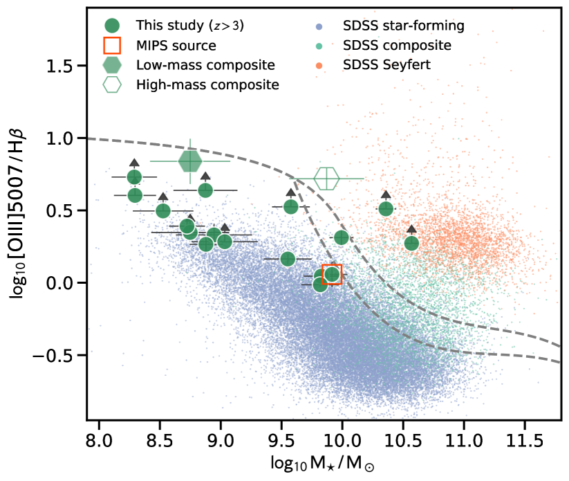
Figure 10: The MEx diagram for spectroscopically identified EELGs at $z\simeq 3.3$ (large circles). The red square indicates a MIPS 24 µm source. Measurements on the low-mass and high-mass composite spectra are shown with filled and open hexagons, respectively. Small dots are galaxies from OSSY SDSS DR7 catalog (Oh et al., 2011) classified as star-forming (blue), composite (green), and Seyfert (orange) galaxies using the BPT diagram (Kauffmann et al., 2003; Kewley et al., 2006). Dashed lines indicate the demarcation lines derived by (Juneau et al., 2014) to separate star-forming, composite, and Seyfert galaxies.

In summary, looking at various possible diagnostics of AGN for our sample, we conclude that EELGs at $z\simeq 3.3$ are most likely to be dominated by star formation, though we cannot completely rule out the presence of AGN at massive end ($M_{\star}\gtrsim 10^{10.5}\,M_{\odot}$). In the following analysis, we consider the all spectroscopically identified EELGs at $z\simeq 3.3$ as SFGs.

5.3 Are EELGs at $z\simeq 3.3$ on the main-sequence of star-forming galaxies?

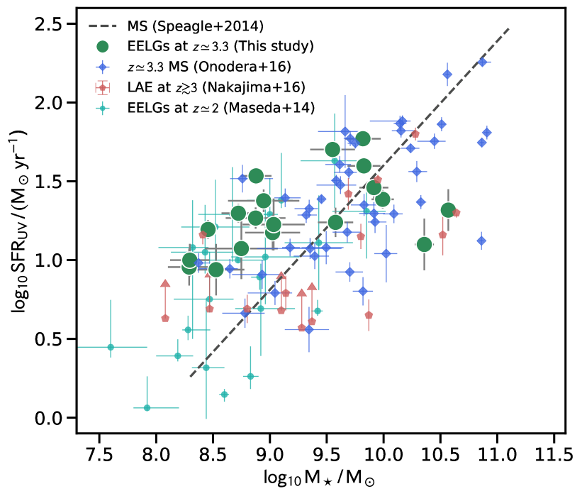
Figure 11: SFR as a function of stellar mass. Green circles show our EELG sample at $z\simeq 3.3$, small light green circles show EELGs at $1.3<z<2.3$ (Maseda et al., 2014), blue diamonds show UV continuum selected SFGs at $z\simeq 3.3$ (Onodera et al., 2016), and red diamonds show $\text{Ly}\alpha$ emitters at $z=3$–$4$ (Nakajima et al., 2016). The dashed line indicates the MS at $z\simeq 3.3$ Speagle et al. (2014).

Figure 11 shows the relation between SFR and stellar mass for our EELG sample at $z\simeq 3.3$ together with normal star-forming galaxies at $z\simeq 3.3$ selected via UV-continuum brightness or expected $\text{H}\beta$ flux (Onodera et al., 2016) and $\text{Ly}\alpha$ emitters (LAEs) at $z=3$–$4$ studied by Nakajima et al. (2016). Objects taken from Nakajima et al. (2016) and Onodera et al. (2016) distribute around the fiducial MS of SFGs at $z\simeq 3.3$ (Speagle et al., 2014). While our spectroscopically identified EELGs at $z\simeq 3.3$ are on the MS at $\log M/M_{\odot}\gtrsim 9.5$, those with $\log M/M_{\odot}\lesssim 9.0$ clearly show higher SFR than the MS by $\gtrsim 0.5$–$1$ dex.

The elevated SFR relative to the MS in less massive galaxies is also seen in EELGs at $1.3<z<2.3$ identified by Maseda et al. (2014) as also shown in Figure 11 with light green circles. They conclude that the star formation in low mass galaxies producing intense [O III] and $\text{H}\alpha$ emission lines is undergoing a burst-like stage with a time scale of $\sim 50$ Myr. The mass-weighted age from the SED fitting with CIGALE for our EELG sample are indeed young, $\simeq 10$–$100$ Myr, at $\log M/M_{\odot}\lesssim 9.0$. Such young stellar population ages for low-mass galaxies are also reported by van der Wel et al. (2011) for a sample of starbursting EELGs at $z\simeq 1.7$ with $\log M/M_{\odot}\simeq 8$. Cohn et al. (2018) carried out an analysis of SFH for EELGs at $2.5<z<4$ and found the evidence of a recent starburst within 50 Myr, which is also a consistent picture with other lower redshift EELGs as well as this study. Therefore, we conclude that low-mass EELGs at $z\simeq 3.3$ are also likely to be in a starburst phase with a short time scale of $\lesssim 100$ Myr.

Although our low-mass EELGs at $z\simeq 3.3$ show similar nature to lower redshift counterparts in the SFR–$M_{\star}$ diagram and stellar ages, one should keep in mind that our EELG selection at a fainter magnitude of $\mathit{Ks}^{\text{obs}}\gtrsim 23$ may fail to select objects located between the EW cut of $\Delta m_{\mathit{Ks}}=0.3$ and the $3\sigma$ cut shown as the dash-dotted and upper solid line, respectively, in Figure 1. This means that the systematic trend of elevated SFR for low-mass EELGs at $z\simeq 3.3$ relative to the MS could be at least partly due to a selection bias. However, it is not straightforward to quantify the bias for [O III] emitters, because translating [O III] flux to SFR (or Balmer line fluxes) is a complex function of various physical parameters such as the gas-phase metallicity, ionization parameter, hardness of UV radiation field, and electron density (Kewley et al., 2013), and also $\mathit{Ks}^{\text{obs}}$ is a combination of emission lines and stellar continuum (i.e., stellar mass). The [O III]/$\text{H}\alpha$ ratios derived by Faisst et al. (2016) using local analogs show a broad distribution of $\log\text{[{O~{}III}]}/\text{H}\alpha\simeq-0.4$–$0.4$ which is also consistent with the range measured for SFGs at $z\simeq 2$ from the literature (e.g., Steidel et al., 2014; Shapley et al., 2015; Suzuki et al., 2016). On the other hand, as we will show in Section 5.4.1, our spectroscopically identified low-mass EELGs follow the $\text{EW}(\text{[{O~{}III}]}\lambda 5007)$–$M_{\star}$ relation defined for more massive normal SFGs at $z\simeq 3.3$ (Reddy et al., 2018a). Therefore, it is not likely that we miss a large amount of low-mass EELGs with significantly lower $\text{EW}(\text{[{O~{}III}]}\lambda 5007)$ because of increasing photometric errors at the fainter magnitude.

5.4 Relation between physical parameters

5.4.1 [O III]$\lambda$5007 equivalent width and SED properties

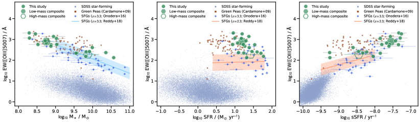
Figure 12: Rest-frame equivalent width of $\text{[{O~{}III}]}\lambda 5007$ as functions of stellar mass (left), SFR (middle), and sSFR (right). Large green filled circles, filled hexagon, and open hexagon show our individual, low-mass composite, and high-mass composite EELGs at $z\simeq 3.3$, respectively. Small dots correspond to local SFGs (Oh et al., 2011), blue diamonds show normal SFGs at $z\simeq 3.3$ taken from Onodera et al. (2016), and filled regions show the relations derived by Reddy et al. (2018a) at $z\simeq 3.3$ in the left panel and at $z\simeq 2.3$ in the middle and right panels.

Figure 12 compares $\text{EW}(\text{[{O~{}III}]}\lambda 5007)$ with SED properties, namely, stellar mass, SFR, and sSFR for our EELGs at $z\simeq 3.3$ (both individual and composite measurements) and other SFGs from the literature, namely local SFGs selected from SDSS (Oh et al., 2011), GPs at $z\simeq 0.2$ (Cardamone et al., 2009), and normal SFGs on the MS at $z\simeq 3.3$ (Onodera et al., 2016). We also compare them with the best-fit relationship derived by Reddy et al. (2018a) for SFGs at $z\simeq 2.3$ and $3.3$.

At a fixed stellar mass, SFGs at $z\simeq 3.3$ from this study, Onodera et al. (2016), and Reddy et al. (2018a) show elevated $\text{EW}(\text{[{O~{}III}]}\lambda 5007)$ by $\simeq 1.5$ dex compared to local SFGs selected from SDSS (Oh et al., 2011) as shown in the left panel of Figure 12. This strong redshift evolution of the $\text{EW}(\text{[{O~{}III}]}\lambda 5007)$–$M_{\star}$ relation for normal SFGs has been reported before (e.g., Khostovan et al., 2016) and the amount of the evolution in our study is similar to their result. The linear relation for a sample of SFGs at $z\simeq 3.4$ is derived at $\log M_{\star}/M_{\odot}\gtrsim 9.5$ by Reddy et al. (2018a). They argued that the evolution of the $\text{EW}(\text{[{O~{}III}]}\lambda 5007)$–$M_{\star}$ relation for the bulk of the SFG population can be explained by the redshift evolution of the SFR–$M_{\star}$ and mass–metallicity relation. Our EELG sample at $z\simeq 3.3$ with $\log M_{\star}/M_{\odot}\lesssim 9$ appears to follow the same relation extrapolated to lower stellar masses, indicating that EELGs may be no longer a rare galaxy population of SFGs at $z\gtrsim 3$, especially at the low stellar masses. On the other hand, EELGs are a rare population in the local universe. Cardamone et al. (2009) estimated the spatial number density of GPs as 2 deg^-2 with $\mathit{r}<20.5$ mag. Only looking at GPs, their $\text{EW}(\text{[{O~{}III}]}\lambda 5007)$–$M_{\star}$ relation is similar to that of EELGs and normal SFGs at $z\simeq 3.3$.

On the other hand, our EELG sample at $z\simeq 3.3$ shows up to $\simeq 3$ dex and $\simeq 1.5$ dex higher $\text{EW}(\text{[{O~{}III}]}\lambda 5007)$ at a fixed SFR compared to those of local and $z\simeq 2.3$ SFGs, respectively (middle panel of Figure 12), while the trend for GPs is quite similar to our EELGs sample showing elevated $\text{EW}(\text{[{O~{}III}]}\lambda 5007)$ at a given SFR. Since Reddy et al. (2018a) used SFR based on $\text{H}\alpha$ luminosity, they did not present the relationship at $z\gtrsim 3$ where $\text{H}\alpha$ falls longer wavelength than the K-band coverage. At $z\simeq 3.3$, the MS does not seem to evolve much since $z\simeq 2.3$. For example, the formula provided by Speagle et al. (2014) suggests a $\simeq 0.1$ dex increase of the normalization of the MS from $z=2.3$ to $z=3.3$. Suzuki et al. (2015) indeed found no difference in the normalization of the MS between narrow-band selected $\text{H}\alpha$ emitters at $z=2.2$ and $2.5$ and [O III] emitters $z=3.2$ and $3.6$, respectively. Note that most of their narrow-band selected objects are normal SFGs at the corresponding redshifts as the narrow-band method selects those with less extreme emission line strengths than the broad-band excess method we applied. This is also confirmed by the distribution of normal SFGs on the MS (Onodera et al., 2016) which is on average consistent with the best-fit relation at $z\simeq 2.3$ by Reddy et al. (2018a). In addition, the average $\text{EW}(\text{[{O~{}III}]}\lambda 5007)$ for SFGs show little evolution at $z\simeq 2$–$3$ (Khostovan et al., 2016). Therefore, the elevated $\text{EW}(\text{[{O~{}III}]}\lambda 5007)$ of our EELG sample as well as GPs can not seem to be explained simply by the evolution of normal SFG population between $z\simeq 3.3$ to $2.3$.

Combining the above two parameters, the right panel of Figure 12 shows the relationship between $\text{EW}(\text{[{O~{}III}]}\lambda 5007)$ and sSFR. EELGs at $z\simeq 3.3$ show elevated $\text{EW}(\text{[{O~{}III}]}\lambda 5007)$ at a fixed sSFR relative to normal SFGs at $z\simeq 3.3$ (Onodera et al., 2016) and those at $z\simeq 2.3$ (Reddy et al., 2018a), while the slope of the relationship does not appear to be very different between two epochs. This trend can also be seen for GPs. Those with lower sSFR of $\lesssim 10^{-8}\,\text{yr}^{-1}$ appear to show more elevation of $\text{EW}(\text{[{O~{}III}]}\lambda 5007)$ at a given sSFR than our EELG sample. More spectroscopic sample of EELGs at $z\simeq 3.3$ would be required for the detailed comparison between high redshift EELGs and local counterparts at this sSFR range. Low-mass objects in our EELG sample with $\log M_{\star}/M_{\odot}<9$ tend to cluster around the upper right part of the figure as also seen from the low-mass composite point. Normal SFGs at $z\simeq 3.3$ presented by Onodera et al. (2016) also contain objects with elevated sSFR of $\log\text{sSFR}/\text{yr}^{-1}\gtrsim-8$ and $\text{EW}(\text{[{O~{}III}]}\lambda 5007)$ of $\gtrsim 500\,\text{\AA}$ similar to our EELGs sample. As seen in the left panel of the figure, most of them are low-mass objects with $\log M_{\star}/M_{\odot}\lesssim 9$.

Sanders et al. (2020b) studied low-mass galaxies with $\log M_{\star}/M_{\odot}\lesssim 9$ at $z=1.5$–$3.5$ with detected auroral $\text{[{O~{}III}]}\lambda 4363$ emission lines to derive robust metallicities via the direct method. Their sample also shows SFR above the MS at $z\simeq 2.3$ and elevated $\text{EW}(\text{[{O~{}III}]}\lambda 5007)$ similar to our EELGs at $z\simeq 3.3$. They concluded that the auroral-line sample is younger and more metal-poor than normal galaxies on the MS. EELGs at $1.3<z<2.4$ presented by Tang et al. (2019) also occupy similar parameter space to the auroral-line sample by Sanders et al. (2020b). Therefore, our EELGs at $z\simeq 3.3$, especially low-mass ones, are also likely to be made of galaxies that are young and low-metallicity and would be promising candidates for a systematic $\text{[{O~{}III}]}\lambda 4363$ follow-up spectroscopic observation. As an example, assuming an electron density of $n_{\text{e}}=500\,\text{cm}^{-3}$ and an electron temperature of $T_{\text{e}}=15000\,\text{K}$ which are reasonable values for high redshift low metallicity SFGs (e.g., Shirazi et al., 2014; Kojima et al., 2017; Sanders et al., 2020b), $\text{[{O~{}III}]}\lambda 4363$ flux is derived as $\simeq 2$ % of the $\text{[{O~{}III}]}\lambda 5007$ flux by using PyNeb (Luridiana et al., 2015). Scaling from a typical $\text{[{O~{}III}]}\lambda 5007$ flux of our EELG sample of $\simeq 10^{-16}\,\text{erg}\,\text{s}^{-1}\,\text{cm}^{-2}$, their $\text{[{O~{}III}]}\lambda 4363$ flux is estimated to be $\simeq 2\times 10^{-18}\,\text{erg}\,\text{s}^{-1}\,\text{cm}^{-2}$. Our Subaru/MOIRCS setup detected the aforementioned $\text{[{O~{}III}]}\lambda 5007$ flux with the $S/N\simeq 20$–$30$ with a $\simeq 1.5$ hr integration. Then it will require $\gtrsim 50$–$100$ hours of telescope time to detect $\text{[{O~{}III}]}\lambda 4363$ with $3\sigma$ significance from individual objects with the same instrument setup. Therefore, the follow-up observation of $\text{[{O~{}III}]}\lambda 4363$ for the EELG sample with Subaru/MOIRCS appears to be impractically expensive, and such observations can be made more efficiently with telescopes with larger apertures on the ground and those in space.

5.4.2 ISM ionization properties

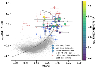
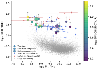
Figure 13: $O_{32}$ as functions of $R_{23}$ (Left) and stellar mass (Right). Our EELGs sample at $z\simeq 3.3$ is shown with large circles color-coded by $\text{EW}(\text{[{O~{}III}]}\lambda 5007)$. The composite values are also shown with a hexagon with a vertex pointing straight across and one with a vertex pointing directly up for the low-mass and high-mass composites, respectively. Local SFGs selected from SDSS (Oh et al., 2011) are shown with small gray dots. Normal continuum-selected SFGs at $z\simeq 3.3$ (Onodera et al., 2016) are shown with small blue diamonds, while LAEs at $z\simeq 3.1$ (Nakajima et al., 2020) are shown with small red pentagons. In the left panel, the solid line indicates the relation between $O_{32}$ and $R_{23}$ presented by Maiolino et al. (2008) with small black squares indicating $12+\log(\text{O/H})=7.5,8.0,8.5,\text{and},9.0$ from top to bottom.

Figure 13 shows $O_{32}$ as functions of $R_{23}$ (left panel) and stellar mass (right panel). $O_{32}$ is an indicator of the ionization parameter (e.g., McGaugh, 1991; Kewley & Dopita, 2002) and $R_{23}$ is a strong-line gas-phase metallicity indicator (e.g., Pagel et al., 1979; Kobulnicky & Phillips, 2003). Compare to local SFGs from SDSS DR7 (Oh et al., 2011), our EELG sample at $z\simeq 3.3$ occupies the upper part of the plot, which means that they are more metal-poor and have higher ionization parameters. The solid line in the left panel of Figure 13 is the locally defined relation of the two line ratios presented by Maiolino et al. (2008) as a function of gas-phase oxygen abundance, $12+\log(\text{O/H})$. Small squares on the line of the local relationship indicate $12+\log(\text{O/H})=7.5,8.0,8.5,\text{and},9.0$. While the majority of local galaxies have $12+\log(\text{O/H})\simeq 8.5$–$9.0$, our EELGs appear to show $R_{23}$ consistent with $12+\log(\text{O/H})=7.5$–$8.5$. EELGs at $z\simeq 3.3$ also show higher ionization parameters compared to those of local SFGs. The observed increase of $\simeq 1$ dex in $O_{32}$ from $z=0$ to $z\simeq 3.3$ can be translated to an increase of $\gtrsim 1.5$ dex in the ionization parameter (e.g., Nakajima & Ouchi, 2014)

In the figure, we also show normal SFGs at $z\simeq 3.3$ (Onodera et al., 2016) and LAEs at $z\simeq 3.1$ (Nakajima et al., 2020). As shown in Nakajima & Ouchi (2014) and seen in the figure, LAEs at $z=2$–$3$ tend to show higher $O_{32}$ indices than normal SFGs at $z\simeq 2$–$3$. The $O_{32}$ of our entire EELGs sample at $z\simeq 3.3$ appears to be distributed between the two populations.

It is also noticeable that EELGs with higher $O_{32}$ values are more likely to show larger $\text{EW}(\text{[{O~{}III}]}\lambda 5007)$. As shown in Figure 12, there is an anti-correlation between $\text{EW}(\text{[{O~{}III}]}\lambda 5007)$ and galaxy stellar mass. Massive EELGs at $z\simeq 3.3$ with $\log M_{\star}/M_{\odot}\gtrsim 9.5$ typically have $\text{EW}(\text{[{O~{}III}]}\lambda 5007)\lesssim 300$ Å, while lower mass ones show $\text{EW}(\text{[{O~{}III}]}\lambda 5007)\gtrsim 500$ Å. From the right panel of Figure 13, it is clearer that at $z\gtrsim 3$ the distribution of the two line ratios considered here for massive EELGs are similar to normal SFGs and that for low-mass ones are closer to LAEs (see also Suzuki et al., 2017). These trends are also seen for the composite measurements.

5.4.3 Ionizing photon production efficiency

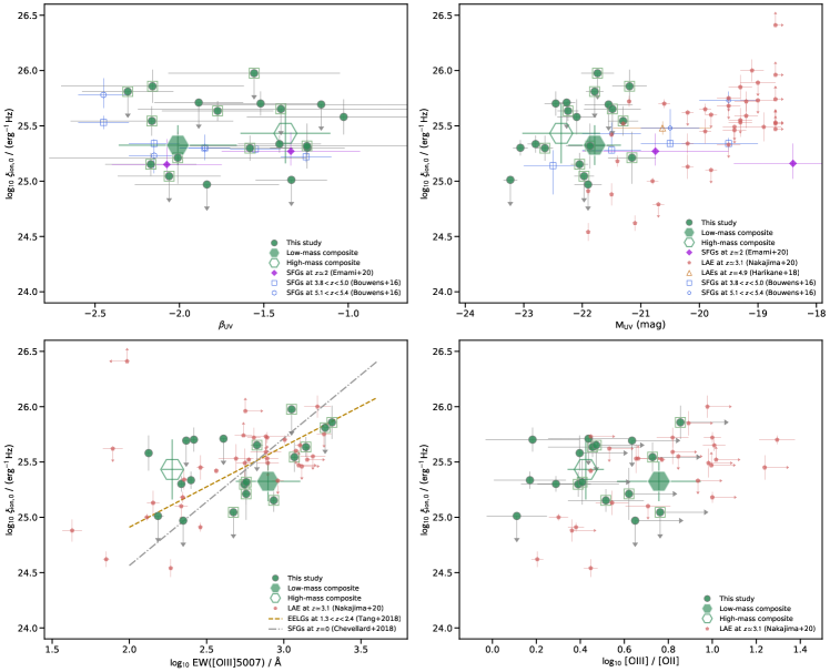
Figure 14: The ionizing photon production efficiency $\xi_{\text{ion,0}}$ as a function of the UV spectral slope $\beta_{\text{UV}}$ (Top Left), the absolute UV magnitude at 1500 Å $M_{\mathrm{UV}}$ (Top Right), $\text{EW}(\text{[{O~{}III}]}\lambda 5007)$ (Bottom Left), and $O_{32}$ (Bottom Right). Our EELGs at $z\simeq 3.3$ are shown with green circles and those with $\log M_{\star}/M_{\odot}\lesssim 9$ are highlighted with squares. Filled and open hexagons represent the low-mass and high-mass composites of the sample, respectively. Filled diamonds show stacked measurements of low-mass SFGs at $1.4<z<2.7$ (Emami et al., 2020). We adopt their Standard stacking, and plot the mid points of each bin along the horizontal axes taken from their Table 1. LAEs at $z=3.1$ taken from Nakajima et al. (2020) are shown with small red pentagons. Measurements for color-selected SFGs at $3.8<z<5.0$ and $5.1<z<5.4$ from Bouwens et al. (2016) are shown with open blue squares and hexagons, respectively. A stacked measurement for LAEs at $z=4.9$ are shown with an open triangle (Harikane et al., 2018). The relationship derived for EELGs at $1.3<z<2.4$ (Tang et al., 2019) is shown with the dashed line. When provided, we consistently used values for the SMC curve for dust correction.

In the upper left panel of Figure 14, we compare $\xi_{\text{ion,0}}$ as a function of $\beta_{\text{UV}}$. Our EELG sample at $z\simeq 3.3$ shows a flat relation between the two parameters with a median value of $\log\xi_{\text{ion,0}}/(\text{erg}^{-1}\,\text{Hz})=25.54$, though 8 out of 19 objects have upper limits for $\xi_{\text{ion,0}}$. This is also the case for the composite spectra. Emami et al. (2020) have found a similar trend, i.e., no $\beta_{\text{UV}}$ dependence of $\xi_{\text{ion,0}}$ for a sample of low-mass ($M_{\star}=10^{7.8}$–$10^{9.8}\,M_{\odot}$) galaxies at $z\simeq 2$ (see also Matthee et al., 2017, for a sample of $\text{H}\alpha$ emitters). They corrected dust attenuation by using the SMC curve for the UV luminosity from SED fitting and the Milky Way (MW) extinction curve (Cardelli et al., 1989) for the $\text{H}\alpha$ luminosity based on the Balmer decrement. On the other hand, different trends have also been reported in the literature. Bouwens et al. (2016) reported a $\simeq 0.3$ dex increase of mean $\xi_{\text{ion,0}}$ for the bluest galaxies ($\beta_{\text{UV}}<-2.3$) for a sample of sub-$L^{*}$ SFGs at $z=4$–$5$, while a constant value of $\log\xi_{\text{ion,0}}/(\text{erg}^{-1}\,\text{Hz})=25.34$ was measured at $\beta_{\text{UV}}>-2.3$. Their conclusion was not affected by the choice of the dust attenuation curve (Calzetti or SMC). Shivaei et al. (2018) found a similar trend to Bouwens et al. (2016) for a sample of SFGs at $z\sim 2$ from the MOSDEF survey (Kriek et al., 2015) using the Calzetti curve for dust correction. When using the SMC curve, their relationship becomes almost flat with a minimum of $\xi_{\text{ion,0}}$ at $\beta_{\text{UV}}\simeq-1.5$ (Shivaei et al., 2018).

To check whether our result changes by using the Calzetti curve instead of the SMC curve, we derived $\xi_{\text{ion,0}}$ assuming the Calzetti curve for stellar continuum following the conversion from $\beta_{\text{UV}}$ to $E{(\mathit{B}-\mathit{V})}_{\text{star}}$ presented in Reddy et al. (2018b), and the MW extinction curve for nebular emission lines with a conversion ${E(\mathit{B}-\mathit{V})}_{\text{neb,MW}}=1.34{E(\mathit{B}-\mathit{V})}_{\text{star,Calz}}$ derived by Theios et al. (2019). Similar to Shivaei et al. (2018), $\xi_{\text{ion,0}}$ becomes $0.1$–$0.4$ dex smaller with the Calzetti curve for dust correction than with the SMC curve with a median difference of $0.28$ dex. The difference appears to become larger for higher $\beta_{\text{UV}}$ objects as also reported by Shivaei et al. (2018), but there seems still no correlation between $\xi_{\text{ion,0}}$ and $\beta_{\text{UV}}$, likely to be partly due to the small number statistics with a large number of upper limits and a relatively large scatter of the distribution of the sample. In addition to the choice of the attenuation curves for dust correction, the conversion factor between the nebular to stellar $E{(\mathit{B}-\mathit{V})}$ could be functions of galaxy properties such as stellar mass, SFR, and hence sSFR as seen in the local universe (Koyama et al., 2019). Although it is not clear whether such relation can be applicable to galaxies at $z\simeq 3.3$ with intense [O III] emission lines, this would potentially introduce an additional uncertainty in $\xi_{\text{ion,0}}$.

The main reason why our EELGs at $z\simeq 3.3$ show no dependence of $\xi_{\text{ion,0}}$ on $\beta_{\text{UV}}$ could be their selection as the most intense $\text{[{O~{}III}]}+\text{H}\beta$ emitting objects. Unlike our selection method, other studies mentioned above did not impose any cuts in emission line strengths. In fact, objects with $\log\xi_{\text{ion,0}}/(\text{erg}^{-1}\,\text{Hz})\simeq 26$ exist at all $\beta_{\text{UV}}$ up to $\beta_{\text{UV}}\simeq-1$ in the tail of the distribution in Shivaei et al. (2018).

The $\xi_{\text{ion,0}}$ of our EELG sample as well as those of SFGs at $z\simeq 2$ (Emami et al., 2020), LAEs at $z\simeq 3.1$ (Nakajima et al., 2020), SFGs at $z\simeq 4$–$5$ (Bouwens et al., 2016), and LAEs at $z=4.9$ (Harikane et al., 2018) are shown as a function of UV absolute magnitude $M_{\text{UV}}$ in the upper right panel of Figure 14. LAEs at $z=4.9$ from Harikane et al. (2018) follow the trend of the $\xi_{\text{ion,0}}$–$M_{\text{UV}}$ relation of SFGs at $z\simeq 4$–$5$ (Bouwens et al., 2016, see also Lam et al. 2019). Our EELGs at $z\simeq 3.3$ show relatively bright $M_{\text{UV}}$ similar to brighter objects of Bouwens et al. (2016), but have on average higher $\xi_{\text{ion,0}}$ by up to $\simeq 0.8$ dex. This may be also an indication of the extreme nature of our sample based on the selection with significant K-band excesses.

Comparing to LAEs at $z\simeq 3.1$ from Nakajima et al. (2020), our EELGs show a similar range of $\xi_{\text{ion,0}}$, but brighter UV luminosities by $2$–$3$ mag despite the similar stellar mass range. A part of the large difference in $M_{\text{UV}}$ could be due to the assumption of a uniform $E{(\mathit{B}-\mathit{V})}_{\text{star}}=0.01$ based on the SED fitting by Fletcher et al. (2019). Note, however, that even a small increase of the dust attenuation parameter can result in a significant increase of the UV luminosity especially when using the SMC extinction curve. If we assume that our EELGs are extinction free, $M_{\text{UV}}$ becomes fainter on average by $\simeq 1.1$ mag. Therefore, the difference in dust correction methods cannot fully explain the difference in UV luminosities between two samples and the reason why the LAE selection can pick up fainter objects with similar stellar masses. Another possible reason of the difference is that Fletcher et al. (2019) performed the SED fitting by using BPASS v2.1 stellar population models (Eldridge et al., 2017), while we adopted BC03 models in the CIGALE framework. Eldridge et al. (2017) pointed out that BC03 models are redder in UV at very young ages of $<10$ Myr and also redder in red-optical to near-IR wavelength at ages more than a few times $100$ Myr. The choice of different population synthesis models can result in a systematic effect in estimating stellar masses. SFGs at $z\simeq 2$ by Emami et al. (2020) include objects with much fainter UV luminosities, $M_{\text{UV}}\gtrsim-18$ and they found no correlation between $\xi_{\text{ion,0}}$ and $M_{\text{UV}}$ in contrast to Nakajima et al. (2020). Note that to derive the UV luminosities Emami et al. (2020) used BC03 templates and the SMC curve for dust correction which are different from those used in Nakajima et al. (2020), and that Emami et al. sample shows on average smaller $\text{EW}(\text{[{O~{}III}]}\lambda 5007)$ of $\simeq 100$ Å than that of Nakajima et al. (2020) of $600$–$1000$ Å, which may be reasons of the discrepancy at the faintest UV magnitude bin.

A strong correlation between $\xi_{\text{ion,0}}$ and $\text{EW}(\text{[{O~{}III}]})$ has been claimed for high redshift EELGs (Emami et al., 2020; Tang et al., 2019; Nakajima et al., 2020) as well as nearby SFGs (Chevallard et al., 2018). The lower left panel of Figure 14 shows the relation between $\xi_{\text{ion,0}}$ and $\text{EW}(\text{[{O~{}III}]}\lambda 5007)$ for our EELG sample at $z\simeq 3.3$ along with that for LAEs at $z\simeq 3.1$ (Nakajima et al., 2020) and the best-fit relations derived for EELGs at $1.3<z<2.4$ (Tang et al., 2019) and for local EELGs (Chevallard et al., 2018). Our EELG sample at $z\simeq 3.3$ follows the similar trend with the relationships in the literature. The correlation between $\xi_{\text{ion,0}}$ and $\text{EW}(\text{[{O~{}III}]})$ appears to be the strongest among four parameters shown in Figure 14. On the other hand, the composite data do not show such correlation. This is probably because we adopted the inverse-variance weighting, which results in putting more weights on objects with the strongest, i.e., the highest S/N, emission line fluxes. As shown in the figure, our EELGs with $\text{EW($\text{[{O~{}III}]}\lambda 5007$)}\gtrsim 300\,\text{\AA}$ are exclusively low-mass galaxies with $\log M_{\star}/M_{\odot}\lesssim 9$, which can also be clearly seen in the composite spectra. Moreover, those with $\text{EW($\text{[{O~{}III}]}\lambda 5007$)}\gtrsim 1000\,\text{\AA}$ show particularly high $\xi_{\text{ion,0}}$ of $\gtrsim 25.5$, suggesting that those with low stellar mass and high $\text{EW}(\text{[{O~{}III}]})$ are very efficient in producing LyC photons.

In the lower right panel of Figure 14, we show the relationship between $\xi_{\text{ion,0}}$ and $O_{32}$. EELGs at $z\simeq 3.3$ do not show an apparent correlation unlike LAEs at $z\simeq 3.1$ (Nakajima et al., 2020) as shown with small red pentagon symbols. Quantitatively, the Spearman’s rank correlation coefficients are 0.05 and 0.48 and the corresponding two-sided p-values are 0.84 and 0.001, for our EELGs at $z\simeq 3.3$ and LAEs at $z\simeq 3.1$, respectively. Shivaei et al. (2018) also found a 0.3 dex enhancement of $\xi_{\text{ion}}$ at large $\log O_{32}\gtrsim 0.5$, while $\xi_{\text{ion}}$ is constant at $\log O_{32}\lesssim 0.5$. They also found that this enhancement can be observed also at low $\log O_{32}$ galaxies when the SMC extinction curve is used for dust correction instead of the Calzetti curve. The systematic effect due to dust correction could be one of the reasons why there is no correlation between $\xi_{\text{ion,0}}$ and $O_{32}$ for our EELG sample. Another reason would be again the biased selection of EELGs as the strongest [O III] emitters. Compared to LAEs at $z\simeq 3.1$, our EELGs show similar $\xi_{\text{ion,0}}$, but systematically lower $O_{32}$ values by $\sim 0.2$ dex, though a relatively large number of objects with only limits hampers a detailed comparison of the distribution of two populations. Because $O_{32}$ can be used as indicators of ionization parameters and gas-phase metallicity (e.g., Maiolino et al., 2008), it is expected that objects with larger $O_{32}$ are efficient hydrogen ionizing photon producers and show elevated $\xi_{\text{ion}}$ values. As seen before, most of the EELGs with larger $\log O_{32}$ of $\gtrsim 0.4$ are low-mass galaxies with $\log M_{\star}/M_{\odot}\lesssim 9$ which follow the distribution of LAEs at a similar redshift well.

In summary, our EELG sample at $z\simeq 3.3$ are efficient hydrogen ionizing photon producers, in particular at lower stellar masses of $\log M_{\star}/M_{\odot}\lesssim 9$. The relationships between $\xi_{\text{ion,0}}$ and various observed properties (Figure 14) suggest that our EELGs have similar properties to luminous SFGs at $z\gtrsim 4$ (Bouwens et al., 2016) and EELGs at $1.4\lesssim z\lesssim 2.5$ (Tang et al., 2019). Comparison with LAEs at $z\simeq 3.1$ indicates that LAEs are systematically less luminous in UV, and more highly ionized objects than the EELGs at $z\simeq 3.3$. Among the investigated parameters, $\xi_{\text{ion,0}}$ of our EELGs show a marginal correlation with $\text{EW}(\text{[{O~{}III}]})$, while other parameters does not impact on the $\xi_{\text{ion,0}}$. This would be mainly due to our biased selection of objects with large $\text{EW}(\text{[{O~{}III}]}+\text{H}\beta)$. Another possible source of systematics is the choice of the attenuation curve for dust correction. If we use the Calzetti curve instead of the SMC curve, $\xi_{\text{ion,0}}$ are reduced by $0.1$–$0.4$ dex. Although the change is more prominent in objects with larger $\beta_{\text{UV}}$, the conclusions of the comparison above are still unchanged. The fact that many of our EELG objects do not have detected $\text{H}\beta$ and $\text{[{O~{}II}]}\lambda 3727$ also dilute correlations if any. A deeper spectroscopic follow-up observation (e.g., Nakajima et al., 2020) is required to make a more detailed comparison.

5.5 Implications for the Lyman continuum escape

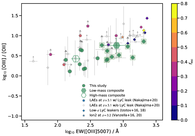
Figure 15: $O_{32}$ as a function of $\text{EW}(\text{[{O~{}III}]}\lambda 5007)$. Our EELGs at $z\simeq 3.3$ are shown as filled green circles of which low mass ($\log M_{\star}/M_{\odot}\lesssim 9$) ones are indicated by open squares. Stacked measurements are shown with open and filled hexagons for low-mass and high-mass composites, respectively. Filled pentagons, diamonds, a small square, and star symbol are previously confirmed from the literature color-coded by LyC escape fraction ($f_{\text{esc}}$); LAEs at $z\simeq 3.1$ (Nakajima et al., 2020),low redshift galaxies at $z\simeq 0.3$ (Izotov et al., 2016, 2018b), and a high redshift LyC leaker at $z=3.2$ (Vanzella et al., 2016, 2020), respectively. Open gray pentagons show LAEs at $z\simeq 3.1$ with no LyC detection (Nakajima et al., 2020).

Our primary motivation to search for EELGs with intense [O III] emission at $z>3$ is to investigate a population of galaxies that can be considered as analogs which contributed to reionize the universe in the EoR as close as possible to the epoch, but not too high redshift where the universe is fully opaque to the LyC emission. Indeed, we have shown that we were able to select such galaxies at $z\simeq 3.3$ with $\text{EW}(\text{[{O~{}III}]}\lambda 5007)$ reaching up to $\simeq 2000\,\text{\AA}$ efficiently by the Ks-band excess method. Such large $\text{EW}(\text{H}\beta+\text{[{O~{}III}]})$ values are comparable to those inferred for SFGs at the EoR (e.g., Smit et al., 2014, 2015; Roberts-Borsani et al., 2016; Stark et al., 2017; De Barros et al., 2019; Endsley et al., 2020).

In addition to such large $\text{EW}(\text{[{O~{}III}]})$, we have shown that the EELG sample at $z\simeq 3.3$ in this study are characterized with enhanced SFR (and sSFR) compared to the MS, large $O_{32}$ values, low level of dust attenuation, bright in UV, and high $\xi_{\text{ion,0}}$, suggesting that they are young, low metallicity galaxies in a bursty phase of star formation with highly ionized ISM. These physical properties are more pronounced in the less massive ones, similar in many aspects to LAEs at a similar redshift and blue SFGs at even higher redshifts as well as EELGs at lower redshifts. Some of these galaxies in the literature are found to show various degrees of LyC escape. Here, we compare observational properties which we have in hand in this study and are considered as indicators of the LyC leakage.

Figure 15 shows the relation between $O_{32}$ and $\text{EW}(\text{[{O~{}III}]}\lambda 5007)$ for our EELG sample at $z\simeq 3.3$ and confirmed LyC leakers at $z\simeq 0.3$ (Izotov et al., 2016, 2018b), and Ion2 at $z=3.2$ (Vanzella et al., 2016, 2020). We also overplot LAEs at $z=3.1$ presented by Nakajima et al. (2020) including those without LyC detection. LyC leakers are color-coded by the LyC escape fraction ($f_{\text{esc}}$). It is notable that there is a large diversity in $f_{\text{esc}}$ among the LyC leakers from a few percent to $>70$ %, and they tend to have large $O_{32}$ values of $\gtrsim 3$–$5$.

Compared to LyC leakers shown in Figure 15, our EELGs follow the similar $O_{32}$–$\text{EW}(\text{[{O~{}III}]}\lambda 5007)$ relationship to confirmed LyC leakers, though many of our EELGs have only lower limits in $O_{32}$ (i.e., non-detection in $\text{[{O~{}II}]}\lambda 3727$). Our EELGs at $z\simeq 3.3$ show large $O_{32}$ values of $\gtrsim 3$ for about a half of the sample and most of them are low-mass galaxies with $\log M_{\star}/M_{\odot}\lesssim 9$ as also seen in the composite measurements. Also, as shown before, these low-mass EELGs show large $\text{EW}(\text{[{O~{}III}]}\lambda 5007)\gtrsim 500$ Å.

The comparison makes it tempting to classify these EELGs at $z\simeq 3.3$ as LyC leakers with large values of $f_{\text{esc}}$. Indeed, photoionization models suggest that $O_{32}$ can be used as an indicator of $f_{\text{esc}}$ (e.g., Jaskot & Oey, 2013; Nakajima & Ouchi, 2014), and observational data also appear to follow the predictions (Faisst et al., 2016, and references therein). However, recent studies suggest that having large $O_{32}$ values is a necessary condition, not a sufficient condition, possibly due to geometrical effects along the line-of-sight (Izotov et al., 2018b; Naidu et al., 2018; Jaskot et al., 2019; Nakajima et al., 2020). Bassett et al. (2019) have made a detailed comparison of the the relation between $f_{\text{esc}}$ and $O_{32}$ with density-bounded models using the MAPPINGS V photoionization code (Allen et al., 2008; Sutherland et al., 2018). They found that $O_{32}$ shows the largest variation at $f_{\text{esc}}<0.1$, while it seems to provide little constraint at larger $f_{\text{esc}}$ than $\simeq 0.1$, especially for low-metallicity cases. The fact that many of LAEs without LyC detections have comparably large $O_{32}$ to LyC leakers also supports these scenarios (Nakajima et al., 2020). Yet, EELGs with very large $O_{32}$ of $\gtrsim 10$ are highly likely to contain LyC leakers, because such high $O_{32}$ ratios can be emerged from a density-bounded nebula (i.e., fully ionized gas cloud) from which LyC emission can escape easily compared to an ionization-bounded nebula where the size of the nebula is determined by the Strömgren sphere (Nakajima & Ouchi, 2014; Jaskot et al., 2019).

Additionally, Bassett et al. (2019) have also discussed that gas-rich galaxy mergers may play a role to break the $O_{32}$–$f_{\text{esc}}$ relation by re-distributing gas in the system. Such mergers of low-mass metal-poor galaxies or inflow of metal-poor gas into the system are suggested to trigger bursty star formation by a sudden change in the gas accretion rate, which could result in breaking the equilibrium of self-regulation of star formation (Lilly et al., 2013; Onodera et al., 2016; Amorín et al., 2017). Alternatively, other mechanisms that are not necessarily classified as mergers but minor interactions and violent disk instabilities, can also produce star-forming clumps and cause mixing of gas in galaxies (Ribeiro et al., 2017). Such clumpy structures are often observed in low-mass metal-poor EELGs at $z<1$ (e.g., Kunth et al., 1988; Lagos et al., 2014; Amorín et al., 2015; Calabrò et al., 2017). Among 11 EELGs in our sample with $\log M_{\star}/M_{\odot}\lesssim 9$, five of them show indications of on-going merger or clumpy structure, while the rest shows compact, point-like morphology in HST/ACS F814W images shown in Figure 16. The apparent diversity of morphology of our EELG sample at $z\simeq 3.3$ could partly reflect different merger stages. Note, however, that these merger- or clumpy-like structures can be due to chance projections along the line-of-sight. In order to fully characterize the nature of individual components of each object, deep high resolution multiband imaging and integral field spectroscopy using currently available facilities such as HST and ground-based 8–10m class telescopes with adaptive optics, and future ones such as James Webb Space Telescope (JWST) and ground-based 30m-class telescopes will be required.

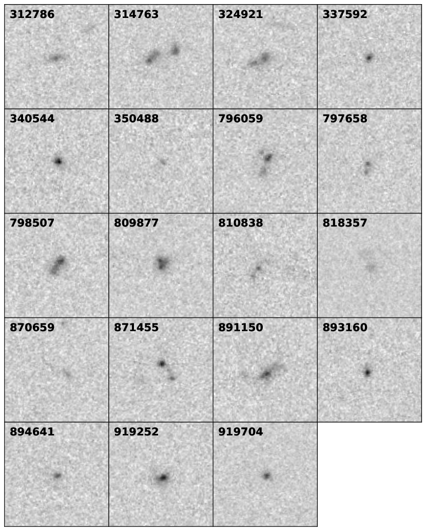
Figure 16: Cutouts of HST/ACS F814W mosaic (Koekemoer et al., 2007; Massey et al., 2010) for the spectroscopically confirmed EELGs at $z\simeq 3.3$. Center of each image corresponds to the coordinate provided in the COSMOS2015 catalog (i.e., measured on the UltraVISTA image), and the size of the image is $3^{\prime}\times 3^{\prime}$. The image is scaled by the arcsinh stretch (Lupton et al., 1999, 2004).

5.6 Implications for galaxies in the epoch of reionization

Whether it is possible for star-forming galaxies in the EoR to provide sufficient hydrogen ionizing photons (i.e., LyC photons) escaped from them is crucial to assess the dominant ionizing population of the reionization. Important parameters here are the hydrogen ionizing photon production efficiency in the case of no LyC escape $\xi_{\text{ion,0}}$ and LyC escape fraction $f_{\text{esc}}$ as the product of the two parameters determines the amount of LyC photons outside of the system. As a canonical value, $\log\xi_{\text{ion,0}}/(\text{erg}^{-1}\,\text{Hz})=25.2$–$25.3$ has been widely used (e.g., Robertson et al., 2013). The value is suggested from BC03 stellar population models at about the solar metallicity with a young stellar population with $\simeq 1$–$10$ Myr old ages for a single burst star formation history. It is also observationally supported by the analysis of $\beta_{\text{UV}}$ slope of galaxies at $z\simeq 7$–$9$ (Dunlop et al., 2013; Robertson et al., 2013).

As seen in Figure 14 and Table 4, the majority of our EELGs at $z\simeq 3.3$ have $\log\xi_{\text{ion,0}}/(\text{erg}^{-1}\,\text{Hz})$ larger than the canonical value, though they include those with upper limits. This means that the majority of our EELGs are more efficiently producing LyC photons than expected by the BC03 models with the aforementioned parameters. Therefore, in order to explain the elevated values of $\xi_{\text{ion,0}}$, different properties of massive stars in galaxies would be needed, such as the IMF, SFH, inclusion of binary populations, and metallicity. Shivaei et al. (2018) have made a detailed investigation on the effect of these parameters using the BPASS and BC03 models. Their fiducial model consists of the Salpeter IMF (Salpeter, 1955) with the lower and upper mass cut of $0.5\,M_{\odot}$ and $100\,M_{\odot}$, respectively, and the slope $\alpha=-2.35$, constant SFH over 300 Myr, $Z=0.15\,Z_{\odot}$, and without binary populations, resulting in $\log\xi_{\text{ion}}/(\text{erg}^{-1}\,\text{Hz})=25.23$. In their analysis, BC03 models with the same parameterization as the fiducial model give $\log\xi_{\text{ion}}/(\text{erg}^{-1}\,\text{Hz})=25.06$, $\sim 0.1$ dex lower than the canonical value mentioned above. Including the binary population, increasing the upper mass cut of IMF to $300\,M_{\odot}$, increasing the IMF slope to $\alpha=-2.00$, and lowering the metallicity to $0.07\,Z_{\odot}$ result in the increase of the $\xi_{\text{ion}}$ by $\sim 0.17$ dex, $\sim 0.16$ dex, $\sim 0.18$ dex, and $0.02$ dex, respectively (see Table 1 in Shivaei et al., 2018). Since our EELGs at $z\simeq 3.3$ typically have $\log\xi_{\text{ion,0}}/(\text{erg}^{-1}\,\text{Hz})\simeq 25.5$ and as large as $\simeq 26.0$, a combination of more than one changes from the fiducial model would be required to explain these values.

In addition to the effects related to their stellar populations as discussed above, the non-zero LyC escape fraction can scale the $\xi_{\text{ion,0}}$ by $1/(1-f_{\text{esc}})$. Statistically speaking, $f_{\text{esc}}=10$–$20$ % is supposed to be necessary for galaxies to fully ionize the universe at $z>6$ (e.g., Ouchi et al., 2009; Robertson et al., 2013), and in this case the intrinsic $\xi_{\text{ion}}$ can be even larger by $\simeq 0.05$–$0.1$ dex. If we simply use the best-fit relation between $O_{32}$ and $f_{\text{esc}}$ derived by Faisst (2016), $f_{\text{esc}}=0.05,0.1$, and $0.45$ correspond to $O_{32}=3,5$, and $10$, respectively, which can be translated to the increase of the intrinsic $\xi_{\text{ion}}$ of 0.02 dex, 0.05 dex, and 0.26 dex, respectively. Therefore, even a moderate escape of LyC from our EELGs can further increase the discrepancy. For those with large values of $O_{32}\simeq 10$ and $\xi_{\text{ion,0}}$, the intrinsic $\xi_{\text{ion}}$ can be as large as $\log\xi_{\text{ion}}/(\text{erg}^{-1}\,\text{Hz})\gtrsim 26$, which cannot be explained even by the most extreme set of parameters for BPASS models considered by Shivaei et al. (2018). As suggested by Figure 11 and Figure 13, even younger stellar population age with a burst-like star formation history, lower metallicity, or a combination of them would be required to explain the most extreme objects in our sample. Note that, as discussed in the previous section, the LyC escape does not seem to be determined solely by the ionization properties inferred by for example $O_{32}$ and $\text{EW}(\text{[{O~{}III}]})$, but the geometry of ionized gas is suggested to be crucial (e.g., Nakajima et al., 2020).

6 Summary

We presented results from a systematic search for EELGs at $z\simeq 3.3$. The selection was done by using the Ks-band excess flux due to intense $\text{H}\beta+\text{[{O~{}III}]}\lambda\lambda 4959,5007$ emission lines relative to the best-fit stellar continuum models. The Ks-excess method was verified successfully by the subsequent near-IR spectroscopic follow-up with Subaru/MOIRCS after the detector upgrade. We observed 23 of 240 Ks-excess objects and identified 21 objects among which 19 galaxies are confirmed to be at $3<z<3.6$ with rest-frame $\text{EW}(\text{[{O~{}III}]}\lambda 5007)>100\,\text{\AA}$ and up to $\simeq 2000\,\text{\AA}$. Focusing on the spectroscopically identified EELGs at $z\simeq 3.3$, we investigated their physical properties derived based both on rich multiband photometry in the COSMOS field and on the MOIRCS near-IR spectra. Our main results can be summarized as follows.

• Photometric redshifts for EELGs at $z\simeq 3.3$ listed in the widely used COSMOS2015 catalog agree with the MOIRCS spectroscopic redshifts, despite the insufficient treatment of nebular emission lines in the catalog. However, stellar masses from the catalog are overestimated for low-mass objects compared to those derived with our dedicated SED fitting including more realistic treatment of the emission line contribution.

• AGN do not seem to dominate the EELG population at $z\simeq 3.3$ judged based on their mid- to far-IR SEDs, emission line widths, and [O III]/$\text{H}\beta$ emission line ratios.

• Our spectroscopically confirmed EELGs at $z\simeq 3.3$ are on the MS at stellar masses of $\gtrsim 10^{9.5}\,M_{\odot}$, while the lower-mass EELGs show elevated SFR than the MS by $\gtrsim 0.5$–$1.0$ dex. This suggests that low-mass EELGs are in a bursty star formation phase with young stellar population age of $\lesssim 100$ Myr.

• EELGs at $z\simeq 3.3$ appear to follow the $M_{\star}$–$\text{EW}(\text{[{O~{}III}]}\lambda 5007)$ relation of normal SFGs at the similar redshift, while at fixed SFR and sSFR they show higher $\text{EW}(\text{[{O~{}III}]}\lambda 5007)$ than normal SFGs at $z\simeq 2.3$ and $3.3$, also supporting the idea that they are young and low metallicity.

• A strong-line metallicity indicator $R_{23}$ indicates that gas-phase metallicity of EELGs at $z\simeq 3.3$ are $12+\log(\text{O/H})=7.5$–$8.5$, while an ionization parameter sensitive index $O_{32}$ shows on average $\sim 1$ dex increase relative to local SFGs, translated to $\gtrsim 1.5$ dex increase of the ionization parameter. Comparison to other galaxy populations at $z\gtrsim 3$, our EELGs show similar ionization properties to normal SFGs at high masses ($\gtrsim 10^{9.5}\,M_{\odot}$) and LAEs at low masses ($\lesssim 10^{9}\,M_{\odot}$).

• The hydrogen ionizing photon production efficiency, $\xi_{\text{ion,0}}$, shows a positive correlation with $\text{EW}(\text{[{O~{}III}]}\lambda\lambda 4959,5007)$. On the other hand, no significant correlation with $\xi_{\text{ion,0}}$ is found for the UV spectral slope, UV luminosity, and $O_{32}$, possibly reflecting the extreme nature of our EELGs compared to objects from the literature with different selections such as LAEs and dropouts.

• Comparison of the $O_{32}$–EW($\text{[{O~{}III}]}\lambda 5007$) relation between our EELG sample and SFGs with measured LyC leakage suggests that our EELGs with the largest $O_{32}$ values of $\gtrsim 10$ and $\text{EW($\text{[{O~{}III}]}\lambda 5007$)}\gtrsim 1000\,\text{\AA}$ likely caused by density-bounded nebulae can be the most promising LyC leaker candidates.

• Our EELGs show $\xi_{\text{ion,0}}$ larger than the commonly used canonical value, suggesting that they are efficient in producing ionizing photons to ionize their surrounding ISM. Considering that $\xi_{\text{ion,0}}$ of our EELG sample at $z\simeq 3.3$ is similar to that of SFGs at higher redshifts of $z>4$–$5$, galaxies at the EoR are likely to have such large values of $\xi_{\text{ion,0}}$ as inferred from the broad-band observations. Assuming an average LyC escape fraction of $\sim 10$ %, intrinsic $\xi_{\text{ion}}$ can become $\log\xi_{\text{ion}}/(\text{erg}^{-1}\,\text{Hz})\gtrsim 26$. In order to reproduce the elevated $\xi_{\text{ion}}$ values, different properties of massive stars in galaxies than the canonical models would be required, including top-heavy IMF, burst-like SFH with younger age, inclusion of binary populations, lower metallicity, or a combination of them.

References

- Alexander et al. (2010) Alexander, D. M., Swinbank, A. M., Smail, I., McDermid, R., & Nesvadba, N. P. H. 2010, MNRAS, 402, 2211, doi: 10.1111/j.1365-2966.2009.16046.x
- Allen et al. (2008) Allen, M. G., Groves, B. A., Dopita, M. A., Sutherland, R. S., & Kewley, L. J. 2008, ApJS, 178, 20, doi: 10.1086/589652
- Amorín et al. (2014) Amorín, R., Grazian, A., Castellano, M., et al. 2014, ApJ, 788, L4, doi: 10.1088/2041-8205/788/1/L4
- Amorín et al. (2015) Amorín, R., Pérez-Montero, E., Contini, T., et al. 2015, A&A, 578, A105, doi: 10.1051/0004-6361/201322786
- Amorín et al. (2017) Amorín, R., Fontana, A., Pérez-Montero, E., et al. 2017, Nature Astronomy, 1, 0052, doi: 10.1038/s41550-017-0052
- Amorín et al. (2010) Amorín, R. O., Pérez-Montero, E., & Vílchez, J. M. 2010, ApJ, 715, L128, doi: 10.1088/2041-8205/715/2/L128
- Astropy Collaboration et al. (2013) Astropy Collaboration, Robitaille, T. P., Tollerud, E. J., et al. 2013, A&A, 558, A33, doi: 10.1051/0004-6361/201322068
- Astropy Collaboration et al. (2018) Astropy Collaboration, Price-Whelan, A. M., Sipőcz, B. M., et al. 2018, AJ, 156, 123, doi: 10.3847/1538-3881/aabc4f
- Atek et al. (2011) Atek, H., Siana, B., Scarlata, C., et al. 2011, ApJ, 743, 121, doi: 10.1088/0004-637X/743/2/121
- Baldwin et al. (1981) Baldwin, J. A., Phillips, M. M., & Terlevich, R. 1981, PASP, 93, 5, doi: 10.1086/130766
- Baskin & Laor (2005) Baskin, A., & Laor, A. 2005, MNRAS, 358, 1043, doi: 10.1111/j.1365-2966.2005.08841.x
- Bassett et al. (2019) Bassett, R., Ryan-Weber, E. V., Cooke, J., et al. 2019, MNRAS, 483, 5223, doi: 10.1093/mnras/sty3320
- Bayliss et al. (2014) Bayliss, M. B., Rigby, J. R., Sharon, K., et al. 2014, ApJ, 790, 144, doi: 10.1088/0004-637X/790/2/144
- Boquien et al. (2019) Boquien, M., Burgarella, D., Roehlly, Y., et al. 2019, A&A, 622, A103, doi: 10.1051/0004-6361/201834156
- Bouwens et al. (2008) Bouwens, R. J., Illingworth, G. D., Franx, M., & Ford, H. 2008, ApJ, 686, 230, doi: 10.1086/590103
- Bouwens et al. (2015) Bouwens, R. J., Illingworth, G. D., Oesch, P. A., et al. 2015, ApJ, 811, 140, doi: 10.1088/0004-637X/811/2/140
- Bouwens et al. (2016) Bouwens, R. J., Smit, R., Labbé, I., et al. 2016, ApJ, 831, 176, doi: 10.3847/0004-637X/831/2/176
- Brammer et al. (2008) Brammer, G. B., van Dokkum, P. G., & Coppi, P. 2008, ApJ, 686, 1503, doi: 10.1086/591786
- Bruzual & Charlot (2003) Bruzual, G., & Charlot, S. 2003, MNRAS, 344, 1000, doi: 10.1046/j.1365-8711.2003.06897.x
- Bunker et al. (1995) Bunker, A. J., Warren, S. J., Hewett, P. C., & Clements, D. L. 1995, MNRAS, 273, 513, doi: 10.1093/mnras/273.2.513
- Burgarella et al. (2005) Burgarella, D., Buat, V., & Iglesias-Páramo, J. 2005, MNRAS, 360, 1413, doi: 10.1111/j.1365-2966.2005.09131.x
- Caccianiga & Severgnini (2011) Caccianiga, A., & Severgnini, P. 2011, MNRAS, 415, 1928, doi: 10.1111/j.1365-2966.2011.18838.x
- Calabrò et al. (2017) Calabrò, A., Amorín, R., Fontana, A., et al. 2017, A&A, 601, A95, doi: 10.1051/0004-6361/201629762
- Calzetti et al. (2000) Calzetti, D., Armus, L., Bohlin, R. C., et al. 2000, ApJ, 533, 682, doi: 10.1086/308692
- Capak et al. (2007) Capak, P., Aussel, H., Ajiki, M., et al. 2007, ApJS, 172, 99, doi: 10.1086/519081
- Cardamone et al. (2009) Cardamone, C., Schawinski, K., Sarzi, M., et al. 2009, MNRAS, 399, 1191, doi: 10.1111/j.1365-2966.2009.15383.x
- Cardelli et al. (1989) Cardelli, J. A., Clayton, G. C., & Mathis, J. S. 1989, ApJ, 345, 245, doi: 10.1086/167900
- Chabrier (2003) Chabrier, G. 2003, PASP, 115, 763, doi: 10.1086/376392
- Chevallard et al. (2018) Chevallard, J., Charlot, S., Senchyna, P., et al. 2018, MNRAS, 479, 3264, doi: 10.1093/mnras/sty1461
- Civano et al. (2016) Civano, F., Marchesi, S., Comastri, A., et al. 2016, ApJ, 819, 62, doi: 10.3847/0004-637X/819/1/62
- Cohn et al. (2018) Cohn, J. H., Leja, J., Tran, K.-V. H., et al. 2018, ApJ, 869, 141, doi: 10.3847/1538-4357/aaed3d
- Daddi et al. (2004) Daddi, E., Cimatti, A., Renzini, A., et al. 2004, ApJ, 617, 746, doi: 10.1086/425569
- Dale & Helou (2002) Dale, D. A., & Helou, G. 2002, ApJ, 576, 159, doi: 10.1086/341632
- De Barros et al. (2019) De Barros, S., Oesch, P. A., Labbé, I., et al. 2019, MNRAS, 489, 2355, doi: 10.1093/mnras/stz940
- de Barros et al. (2016) de Barros, S., Vanzella, E., Amorín, R., et al. 2016, A&A, 585, A51, doi: 10.1051/0004-6361/201527046
- Dijkstra et al. (2016) Dijkstra, M., Gronke, M., & Venkatesan, A. 2016, ApJ, 828, 71, doi: 10.3847/0004-637X/828/2/71
- Dunlop et al. (2013) Dunlop, J. S., Rogers, A. B., McLure, R. J., et al. 2013, MNRAS, 432, 3520, doi: 10.1093/mnras/stt702
- Eldridge et al. (2017) Eldridge, J. J., Stanway, E. R., Xiao, L., et al. 2017, PASA, 34, e058, doi: 10.1017/pasa.2017.51
- Ellis et al. (2013) Ellis, R. S., McLure, R. J., Dunlop, J. S., et al. 2013, ApJ, 763, L7, doi: 10.1088/2041-8205/763/1/L7
- Emami et al. (2020) Emami, N., Siana, B., Alavi, A., et al. 2020, ApJ, 895, 116, doi: 10.3847/1538-4357/ab8f97
- Endsley et al. (2020) Endsley, R., Stark, D. P., Chevallard, J., & Charlot, S. 2020, arXiv e-prints, arXiv:2005.02402. https://arxiv.org/abs/2005.02402
- Fabricius et al. (2016) Fabricius, M., Walawender, J., Arimoto, N., et al. 2016, in Society of Photo-Optical Instrumentation Engineers (SPIE) Conference Series, Vol. 9908, Ground-based and Airborne Instrumentation for Astronomy VI, 990828, doi: 10.1117/12.2231417
- Faisst (2016) Faisst, A. L. 2016, ApJ, 829, 99, doi: 10.3847/0004-637X/829/2/99
- Faisst et al. (2016) Faisst, A. L., Capak, P., Hsieh, B. C., et al. 2016, ApJ, 821, 122, doi: 10.3847/0004-637X/821/2/122
- Fletcher et al. (2019) Fletcher, T. J., Tang, M., Robertson, B. E., et al. 2019, ApJ, 878, 87, doi: 10.3847/1538-4357/ab2045
- Foreman-Mackey et al. (2013) Foreman-Mackey, D., Hogg, D. W., Lang, D., & Goodman, J. 2013, PASP, 125, 306, doi: 10.1086/670067
- Fosbury et al. (2003) Fosbury, R. A. E., Villar-Martín, M., Humphrey, A., et al. 2003, ApJ, 596, 797, doi: 10.1086/378228
- Genzel et al. (2014) Genzel, R., Förster Schreiber, N. M., Rosario, D., et al. 2014, ApJ, 796, 7, doi: 10.1088/0004-637X/796/1/7
- Goodman & Weare (2010) Goodman, J., & Weare, J. 2010, Communications in Applied Mathematics and Computational Science, 5, 65, doi: 10.2140/camcos.2010.5.65
- Gordon et al. (2003) Gordon, K. D., Clayton, G. C., Misselt, K. A., Land olt, A. U., & Wolff, M. J. 2003, ApJ, 594, 279, doi: 10.1086/376774
- Harikane et al. (2018) Harikane, Y., Ouchi, M., Shibuya, T., et al. 2018, ApJ, 859, 84, doi: 10.3847/1538-4357/aabd80
- Harris et al. (2020) Harris, C. R., Millman, K. J., van der Walt, S. J., et al. 2020, Nature, 585, 357, doi: 10.1038/s41586-020-2649-2
- Holt et al. (2008) Holt, J., Tadhunter, C. N., & Morganti, R. 2008, MNRAS, 387, 639, doi: 10.1111/j.1365-2966.2008.13089.x
- Horne (1986) Horne, K. 1986, PASP, 98, 609, doi: 10.1086/131801
- Hunter (2007) Hunter, J. D. 2007, Computing in Science & Engineering, 9, 90, doi: 10.1109/MCSE.2007.55
- Ichikawa et al. (2006) Ichikawa, T., Suzuki, R., Tokoku, C., et al. 2006, in Society of Photo-Optical Instrumentation Engineers (SPIE) Conference Series, Vol. 6269, Society of Photo-Optical Instrumentation Engineers (SPIE) Conference Series, 626916, doi: 10.1117/12.670078
- Inoue (2011) Inoue, A. K. 2011, MNRAS, 415, 2920, doi: 10.1111/j.1365-2966.2011.18906.x
- Inoue & Iwata (2008) Inoue, A. K., & Iwata, I. 2008, MNRAS, 387, 1681, doi: 10.1111/j.1365-2966.2008.13350.x
- Izotov et al. (2011) Izotov, Y. I., Guseva, N. G., & Thuan, T. X. 2011, ApJ, 728, 161, doi: 10.1088/0004-637X/728/2/161
- Izotov et al. (2016) Izotov, Y. I., Orlitová, I., Schaerer, D., et al. 2016, Nature, 529, 178, doi: 10.1038/nature16456
- Izotov et al. (2018a) Izotov, Y. I., Schaerer, D., Worseck, G., et al. 2018a, MNRAS, 474, 4514, doi: 10.1093/mnras/stx3115
- Izotov et al. (2020) —. 2020, MNRAS, 491, 468, doi: 10.1093/mnras/stz3041
- Izotov et al. (2018b) Izotov, Y. I., Worseck, G., Schaerer, D., et al. 2018b, MNRAS, 478, 4851, doi: 10.1093/mnras/sty1378
- Jaskot et al. (2019) Jaskot, A. E., Dowd, T., Oey, M. S., Scarlata, C., & McKinney, J. 2019, ApJ, 885, 96, doi: 10.3847/1538-4357/ab3d3b
- Jaskot & Oey (2013) Jaskot, A. E., & Oey, M. S. 2013, ApJ, 766, 91, doi: 10.1088/0004-637X/766/2/91
- Juneau et al. (2011) Juneau, S., Dickinson, M., Alexander, D. M., & Salim, S. 2011, ApJ, 736, 104, doi: 10.1088/0004-637X/736/2/104
- Juneau et al. (2014) Juneau, S., Bournaud, F., Charlot, S., et al. 2014, ApJ, 788, 88, doi: 10.1088/0004-637X/788/1/88
- Kashikawa et al. (2006) Kashikawa, N., Shimasaku, K., Malkan, M. A., et al. 2006, ApJ, 648, 7, doi: 10.1086/504966
- Kauffmann et al. (2003) Kauffmann, G., Heckman, T. M., White, S. D. M., et al. 2003, MNRAS, 341, 33, doi: 10.1046/j.1365-8711.2003.06291.x
- Kennicutt & Evans (2012) Kennicutt, R. C., & Evans, N. J. 2012, ARA&A, 50, 531, doi: 10.1146/annurev-astro-081811-125610
- Kennicutt (1998) Kennicutt, Jr., R. C. 1998, ARA&A, 36, 189, doi: 10.1146/annurev.astro.36.1.189
- Kewley & Dopita (2002) Kewley, L. J., & Dopita, M. A. 2002, ApJS, 142, 35, doi: 10.1086/341326
- Kewley et al. (2013) Kewley, L. J., Dopita, M. A., Leitherer, C., et al. 2013, ApJ, 774, 100, doi: 10.1088/0004-637X/774/2/100
- Kewley et al. (2001) Kewley, L. J., Dopita, M. A., Sutherland, R. S., Heisler, C. A., & Trevena, J. 2001, ApJ, 556, 121, doi: 10.1086/321545
- Kewley et al. (2006) Kewley, L. J., Groves, B., Kauffmann, G., & Heckman, T. 2006, MNRAS, 372, 961, doi: 10.1111/j.1365-2966.2006.10859.x
- Khostovan et al. (2016) Khostovan, A. A., Sobral, D., Mobasher, B., et al. 2016, MNRAS, 463, 2363, doi: 10.1093/mnras/stw2174
- Kobulnicky & Phillips (2003) Kobulnicky, H. A., & Phillips, A. C. 2003, ApJ, 599, 1031, doi: 10.1086/379361
- Koekemoer et al. (2007) Koekemoer, A. M., Aussel, H., Calzetti, D., et al. 2007, ApJS, 172, 196, doi: 10.1086/520086
- Kojima et al. (2017) Kojima, T., Ouchi, M., Nakajima, K., et al. 2017, PASJ, 69, 44, doi: 10.1093/pasj/psx017
- Komatsu et al. (2011) Komatsu, E., Smith, K. M., Dunkley, J., et al. 2011, ApJS, 192, 18, doi: 10.1088/0067-0049/192/2/18
- Koyama et al. (2019) Koyama, Y., Shimakawa, R., Yamamura, I., Kodama, T., & Hayashi, M. 2019, PASJ, 71, 8, doi: 10.1093/pasj/psy113
- Kriek et al. (2015) Kriek, M., Shapley, A. E., Reddy, N. A., et al. 2015, ApJS, 218, 15, doi: 10.1088/0067-0049/218/2/15
- Kunth et al. (1988) Kunth, D., Maurogordato, S., & Vigroux, L. 1988, A&A, 204, 10
- Kurucz (1979) Kurucz, R. L. 1979, ApJS, 40, 1, doi: 10.1086/190589
- Lagos et al. (2014) Lagos, P., Papaderos, P., Gomes, J. M., Smith Castelli, A. V., & Vega, L. R. 2014, A&A, 569, A110, doi: 10.1051/0004-6361/201323353
- Laigle et al. (2016) Laigle, C., McCracken, H. J., Ilbert, O., et al. 2016, ApJS, 224, 24, doi: 10.3847/0067-0049/224/2/24
- Lam et al. (2019) Lam, D., Bouwens, R. J., Labbé, I., et al. 2019, A&A, 627, A164, doi: 10.1051/0004-6361/201935227
- Leitherer & Heckman (1995) Leitherer, C., & Heckman, T. M. 1995, ApJS, 96, 9, doi: 10.1086/192112
- Lilly et al. (2013) Lilly, S. J., Carollo, C. M., Pipino, A., Renzini, A., & Peng, Y. 2013, ApJ, 772, 119, doi: 10.1088/0004-637X/772/2/119
- Lupton et al. (2004) Lupton, R., Blanton, M. R., Fekete, G., et al. 2004, PASP, 116, 133, doi: 10.1086/382245
- Lupton et al. (1999) Lupton, R. H., Gunn, J. E., & Szalay, A. S. 1999, AJ, 118, 1406, doi: 10.1086/301004
- Luridiana et al. (2015) Luridiana, V., Morisset, C., & Shaw, R. A. 2015, A&A, 573, A42, doi: 10.1051/0004-6361/201323152
- Lutz et al. (2011) Lutz, D., Poglitsch, A., Altieri, B., et al. 2011, A&A, 532, A90, doi: 10.1051/0004-6361/201117107
- Madau (1995) Madau, P. 1995, ApJ, 441, 18, doi: 10.1086/175332
- Maiolino et al. (2008) Maiolino, R., Nagao, T., Grazian, A., et al. 2008, A&A, 488, 463, doi: 10.1051/0004-6361:200809678
- Marchesi et al. (2016) Marchesi, S., Civano, F., Elvis, M., et al. 2016, ApJ, 817, 34, doi: 10.3847/0004-637X/817/1/34
- Marchesini et al. (2010) Marchesini, D., Whitaker, K. E., Brammer, G., et al. 2010, ApJ, 725, 1277, doi: 10.1088/0004-637X/725/1/1277
- Maseda et al. (2014) Maseda, M. V., van der Wel, A., Rix, H.-W., et al. 2014, ApJ, 791, 17, doi: 10.1088/0004-637X/791/1/17
- Massey et al. (2010) Massey, R., Stoughton, C., Leauthaud, A., et al. 2010, MNRAS, 401, 371, doi: 10.1111/j.1365-2966.2009.15638.x
- Matsuoka et al. (2018) Matsuoka, Y., Strauss, M. A., Kashikawa, N., et al. 2018, ApJ, 869, 150, doi: 10.3847/1538-4357/aaee7a
- Matthee et al. (2017) Matthee, J., Sobral, D., Best, P., et al. 2017, MNRAS, 465, 3637, doi: 10.1093/mnras/stw2973
- McCracken et al. (2012) McCracken, H. J., Milvang-Jensen, B., Dunlop, J., et al. 2012, A&A, 544, A156, doi: 10.1051/0004-6361/201219507
- McGaugh (1991) McGaugh, S. S. 1991, ApJ, 380, 140, doi: 10.1086/170569
- Meiksin (2006) Meiksin, A. 2006, MNRAS, 365, 807, doi: 10.1111/j.1365-2966.2005.09756.x
- Naidu et al. (2018) Naidu, R. P., Forrest, B., Oesch, P. A., Tran, K.-V. H., & Holden, B. P. 2018, MNRAS, 478, 791, doi: 10.1093/mnras/sty961
- Nakajima et al. (2016) Nakajima, K., Ellis, R. S., Iwata, I., et al. 2016, ApJ, 831, L9, doi: 10.3847/2041-8205/831/1/L9
- Nakajima et al. (2020) Nakajima, K., Ellis, R. S., Robertson, B. E., Tang, M., & Stark, D. P. 2020, ApJ, 889, 161, doi: 10.3847/1538-4357/ab6604
- Nakajima & Ouchi (2014) Nakajima, K., & Ouchi, M. 2014, MNRAS, 442, 900, doi: 10.1093/mnras/stu902
- Newville et al. (2019) Newville, M., Otten, R., Nelson, A., et al. 2019, lmfit/lmfit-py latest, doi: 0.5281/zenodo.598352
- Noll et al. (2009) Noll, S., Burgarella, D., Giovannoli, E., et al. 2009, A&A, 507, 1793, doi: 10.1051/0004-6361/200912497
- Nordon et al. (2013) Nordon, R., Lutz, D., Saintonge, A., et al. 2013, ApJ, 762, 125, doi: 10.1088/0004-637X/762/2/125
- Oh et al. (2011) Oh, K., Sarzi, M., Schawinski, K., & Yi, S. K. 2011, ApJS, 195, 13, doi: 10.1088/0067-0049/195/2/13
- Oke & Gunn (1983) Oke, J. B., & Gunn, J. E. 1983, ApJ, 266, 713, doi: 10.1086/160817
- Oliver et al. (2012) Oliver, S. J., Bock, J., Altieri, B., et al. 2012, MNRAS, 424, 1614, doi: 10.1111/j.1365-2966.2012.20912.x
- Ono et al. (2018) Ono, Y., Ouchi, M., Harikane, Y., et al. 2018, PASJ, 70, S10, doi: 10.1093/pasj/psx103
- Onodera et al. (2016) Onodera, M., Carollo, C. M., Lilly, S., et al. 2016, ApJ, 822, 42, doi: 10.3847/0004-637X/822/1/42
- Osterbrock & Ferland (2006) Osterbrock, D., & Ferland, G. 2006, Astrophysics Of Gas Nebulae and Active Galactic Nuclei (University Science Books). https://books.google.com/books?id=HgfrkDjBD98C
- Ota et al. (2010) Ota, K., Iye, M., Kashikawa, N., et al. 2010, ApJ, 722, 803, doi: 10.1088/0004-637X/722/1/803
- Ouchi et al. (2009) Ouchi, M., Mobasher, B., Shimasaku, K., et al. 2009, ApJ, 706, 1136, doi: 10.1088/0004-637X/706/2/1136
- Ouchi et al. (2010) Ouchi, M., Shimasaku, K., Furusawa, H., et al. 2010, ApJ, 723, 869, doi: 10.1088/0004-637X/723/1/869
- Ouchi et al. (2018) Ouchi, M., Harikane, Y., Shibuya, T., et al. 2018, PASJ, 70, S13, doi: 10.1093/pasj/psx074
- Pagel et al. (1979) Pagel, B. E. J., Edmunds, M. G., Blackwell, D. E., Chun, M. S., & Smith, G. 1979, MNRAS, 189, 95, doi: 10.1093/mnras/189.1.95
- Pannella et al. (2015) Pannella, M., Elbaz, D., Daddi, E., et al. 2015, ApJ, 807, 141, doi: 10.1088/0004-637X/807/2/141
- Reddy et al. (2016a) Reddy, N. A., Steidel, C. C., Pettini, M., & Bogosavljević, M. 2016a, ApJ, 828, 107, doi: 10.3847/0004-637X/828/2/107
- Reddy et al. (2016b) Reddy, N. A., Steidel, C. C., Pettini, M., Bogosavljević, M., & Shapley, A. E. 2016b, ApJ, 828, 108, doi: 10.3847/0004-637X/828/2/108
- Reddy et al. (2015) Reddy, N. A., Kriek, M., Shapley, A. E., et al. 2015, ApJ, 806, 259, doi: 10.1088/0004-637X/806/2/259
- Reddy et al. (2018a) Reddy, N. A., Shapley, A. E., Sanders, R. L., et al. 2018a, ApJ, 869, 92, doi: 10.3847/1538-4357/aaed1e
- Reddy et al. (2018b) Reddy, N. A., Oesch, P. A., Bouwens, R. J., et al. 2018b, ApJ, 853, 56, doi: 10.3847/1538-4357/aaa3e7
- Ribeiro et al. (2017) Ribeiro, B., Le Fèvre, O., Cassata, P., et al. 2017, A&A, 608, A16, doi: 10.1051/0004-6361/201630057
- Roberts-Borsani et al. (2016) Roberts-Borsani, G. W., Bouwens, R. J., Oesch, P. A., et al. 2016, ApJ, 823, 143, doi: 10.3847/0004-637X/823/2/143
- Robertson et al. (2015) Robertson, B. E., Ellis, R. S., Furlanetto, S. R., & Dunlop, J. S. 2015, ApJ, 802, L19, doi: 10.1088/2041-8205/802/2/L19
- Robertson et al. (2013) Robertson, B. E., Furlanetto, S. R., Schneider, E., et al. 2013, ApJ, 768, 71, doi: 10.1088/0004-637X/768/1/71
- Robitaille (2019) Robitaille, T. 2019, APLpy v2.0: The Astronomical Plotting Library in Python, doi: 10.5281/zenodo.2567476
- Robitaille & Bressert (2012) Robitaille, T., & Bressert, E. 2012, APLpy: Astronomical Plotting Library in Python. http://ascl.net/1208.017
- Rousselot et al. (2000) Rousselot, P., Lidman, C., Cuby, J. G., Moreels, G., & Monnet, G. 2000, A&A, 354, 1134
- Salpeter (1955) Salpeter, E. E. 1955, ApJ, 121, 161, doi: 10.1086/145971
- Sanders et al. (2020a) Sanders, R. L., Shapley, A. E., Jones, T., et al. 2020a, arXiv e-prints, arXiv:2009.07292. https://arxiv.org/abs/2009.07292
- Sanders et al. (2020b) Sanders, R. L., Shapley, A. E., Reddy, N. A., et al. 2020b, MNRAS, 491, 1427, doi: 10.1093/mnras/stz3032
- Schaerer et al. (2013) Schaerer, D., de Barros, S., & Sklias, P. 2013, A&A, 549, A4, doi: 10.1051/0004-6361/201220002
- Scoville et al. (2007) Scoville, N., Aussel, H., Brusa, M., et al. 2007, ApJS, 172, 1, doi: 10.1086/516585
- Shapley et al. (2015) Shapley, A. E., Reddy, N. A., Kriek, M., et al. 2015, ApJ, 801, 88, doi: 10.1088/0004-637X/801/2/88
- Shirazi et al. (2014) Shirazi, M., Brinchmann, J., & Rahmati, A. 2014, ApJ, 787, 120, doi: 10.1088/0004-637X/787/2/120
- Shivaei et al. (2018) Shivaei, I., Reddy, N. A., Siana, B., et al. 2018, ApJ, 855, 42, doi: 10.3847/1538-4357/aaad62
- Smit et al. (2014) Smit, R., Bouwens, R. J., Labbé, I., et al. 2014, ApJ, 784, 58, doi: 10.1088/0004-637X/784/1/58
- Smit et al. (2015) Smit, R., Bouwens, R. J., Franx, M., et al. 2015, ApJ, 801, 122, doi: 10.1088/0004-637X/801/2/122
- Speagle et al. (2014) Speagle, J. S., Steinhardt, C. L., Capak, P. L., & Silverman, J. D. 2014, ApJS, 214, 15, doi: 10.1088/0067-0049/214/2/15
- Stark et al. (2013) Stark, D. P., Schenker, M. A., Ellis, R., et al. 2013, ApJ, 763, 129, doi: 10.1088/0004-637X/763/2/129
- Stark et al. (2017) Stark, D. P., Ellis, R. S., Charlot, S., et al. 2017, MNRAS, 464, 469, doi: 10.1093/mnras/stw2233
- Steidel et al. (2014) Steidel, C. C., Rudie, G. C., Strom, A. L., et al. 2014, ApJ, 795, 165, doi: 10.1088/0004-637X/795/2/165
- Straughn et al. (2008) Straughn, A. N., Meurer, G. R., Pirzkal, N., et al. 2008, AJ, 135, 1624, doi: 10.1088/0004-6256/135/4/1624
- Strom et al. (2018) Strom, A. L., Steidel, C. C., Rudie, G. C., Trainor, R. F., & Pettini, M. 2018, ApJ, 868, 117, doi: 10.3847/1538-4357/aae1a5
- Strom et al. (2017) Strom, A. L., Steidel, C. C., Rudie, G. C., et al. 2017, ApJ, 836, 164, doi: 10.3847/1538-4357/836/2/164
- Sutherland et al. (2018) Sutherland, R., Dopita, M., Binette, L., & Groves, B. 2018, MAPPINGS V: Astrophysical plasma modeling code. http://ascl.net/1807.005
- Suzuki et al. (2008) Suzuki, R., Tokoku, C., Ichikawa, T., et al. 2008, PASJ, 60, 1347, doi: 10.1093/pasj/60.6.1347
- Suzuki et al. (2015) Suzuki, T. L., Kodama, T., Tadaki, K.-i., et al. 2015, ApJ, 806, 208, doi: 10.1088/0004-637X/806/2/208
- Suzuki et al. (2016) Suzuki, T. L., Kodama, T., Sobral, D., et al. 2016, MNRAS, 462, 181, doi: 10.1093/mnras/stw1655
- Suzuki et al. (2017) Suzuki, T. L., Kodama, T., Onodera, M., et al. 2017, ApJ, 849, 39, doi: 10.3847/1538-4357/aa8df3
- Tadaki et al. (2013) Tadaki, K.-i., Kodama, T., Tanaka, I., et al. 2013, ApJ, 778, 114, doi: 10.1088/0004-637X/778/2/114
- Tanaka et al. (2017) Tanaka, M., Hasinger, G., Silverman, J. D., et al. 2017, arXiv e-prints, arXiv:1706.00566. https://arxiv.org/abs/1706.00566
- Tang et al. (2019) Tang, M., Stark, D. P., Chevallard, J., & Charlot, S. 2019, MNRAS, 489, 2572, doi: 10.1093/mnras/stz2236
- Taniguchi et al. (2007) Taniguchi, Y., Scoville, N., Murayama, T., et al. 2007, ApJS, 172, 9, doi: 10.1086/516596
- Taniguchi et al. (2015) Taniguchi, Y., Kajisawa, M., Kobayashi, M. A. R., et al. 2015, PASJ, 67, 104, doi: 10.1093/pasj/psv106
- Taylor (2005) Taylor, M. B. 2005, in Astronomical Society of the Pacific Conference Series, Vol. 347, Astronomical Data Analysis Software and Systems XIV, ed. P. Shopbell, M. Britton, & R. Ebert, 29
- Telles & Melnick (2018) Telles, E., & Melnick, J. 2018, A&A, 615, A55, doi: 10.1051/0004-6361/201732275
- Theios et al. (2019) Theios, R. L., Steidel, C. C., Strom, A. L., et al. 2019, ApJ, 871, 128, doi: 10.3847/1538-4357/aaf386
- Tody (1986) Tody, D. 1986, in Society of Photo-Optical Instrumentation Engineers (SPIE) Conference Series, Vol. 627, Instrumentation in astronomy VI, ed. D. L. Crawford, 733, doi: 10.1117/12.968154
- Tody (1993) Tody, D. 1993, in Astronomical Society of the Pacific Conference Series, Vol. 52, Astronomical Data Analysis Software and Systems II, ed. R. J. Hanisch, R. J. V. Brissenden, & J. Barnes, 173
- Tran et al. (2020) Tran, K.-V. H., Forrest, B., Alcorn, L. Y., et al. 2020, ApJ, 898, 45, doi: 10.3847/1538-4357/ab8cba
- van der Wel et al. (2011) van der Wel, A., Straughn, A. N., Rix, H. W., et al. 2011, ApJ, 742, 111, doi: 10.1088/0004-637X/742/2/111
- Vanzella et al. (2016) Vanzella, E., de Barros, S., Vasei, K., et al. 2016, ApJ, 825, 41, doi: 10.3847/0004-637X/825/1/41
- Vanzella et al. (2020) Vanzella, E., Caminha, G. B., Calura, F., et al. 2020, MNRAS, 491, 1093, doi: 10.1093/mnras/stz2286
- Verhamme et al. (2015) Verhamme, A., Orlitová, I., Schaerer, D., & Hayes, M. 2015, A&A, 578, A7, doi: 10.1051/0004-6361/201423978
- Walawender et al. (2016) Walawender, J., Wung, M., Fabricius, M., et al. 2016, in Society of Photo-Optical Instrumentation Engineers (SPIE) Conference Series, Vol. 9908, Ground-based and Airborne Instrumentation for Astronomy VI, 99082G, doi: 10.1117/12.2231812
- Waskom et al. (2020) Waskom, M., Botvinnik, O., Ostblom, J., et al. 2020, mwaskom/seaborn: latest, latest, Zenodo, doi: 10.5281/zenodo.592845
- Whitaker et al. (2014) Whitaker, K. E., Franx, M., Leja, J., et al. 2014, ApJ, 795, 104, doi: 10.1088/0004-637X/795/2/104
- Wuyts et al. (2016) Wuyts, E., Wisnioski, E., Fossati, M., et al. 2016, ApJ, 827, 74, doi: 10.3847/0004-637X/827/1/74
- Wuyts et al. (2008) Wuyts, S., Labbé, I., Förster Schreiber, N. M., et al. 2008, ApJ, 682, 985, doi: 10.1086/588749
- Yamada et al. (2005) Yamada, S. F., Sasaki, S. S., Sumiya, R., et al. 2005, PASJ, 57, 881, doi: 10.1093/pasj/57.6.881
- Yeh & Matzner (2012) Yeh, S. C. C., & Matzner, C. D. 2012, ApJ, 757, 108, doi: 10.1088/0004-637X/757/2/108
- Yoshikawa et al. (2010) Yoshikawa, T., Akiyama, M., Kajisawa, M., et al. 2010, ApJ, 718, 112, doi: 10.1088/0004-637X/718/1/112
- Zahid et al. (2014) Zahid, H. J., Kashino, D., Silverman, J. D., et al. 2014, ApJ, 792, 75, doi: 10.1088/0004-637X/792/1/75