Motif Learning in Knowledge Graphs
using Trajectories Of Differential Equations

Abstract.

Knowledge Graph Embeddings (KGEs) have shown promising performance on link prediction tasks by mapping the entities and relations from a knowledge graph into a geometric space (usually a vector space). Ultimately, the plausibility of the predicted links is measured by using a scoring function over the learned embeddings (vectors). Therefore, the capability in preserving graph characteristics including structural aspects and semantics, highly depends on the design of the KGE, as well as the inherited abilities from the underlying geometry. Many KGEs use the flat geometry which renders them incapable of preserving complex structures and consequently causes wrong inferences by the models. To address this problem, we propose a neuro differential KGE that embeds nodes of a KG on the trajectories of Ordinary Differential Equations (ODEs). To this end, we represent each relation (edge) in a KG as a vector field on a smooth Riemannian manifold. We specifically parameterize ODEs by a neural network to represent various complex shape manifolds and more importantly complex shape vector fields on the manifold. Therefore, the underlying embedding space is capable of getting various geometric forms to encode complexity in subgraph structures with different motifs. Experiments on synthetic and benchmark dataset as well as social network KGs justify the ODE trajectories as a means to structure preservation and consequently avoiding wrong inferences over state-of-the-art KGE models.

1. Introduction

Knowledge Graphs (KGs) have hugely impacted AI-based applications (on and off the Web) such as question answering, recommendation systems, and prediction services (Wang et al., 2017). A KG represents factual knowledge in triples of form (entity, relation, entity) e.g., (Plato, influences, Kant), in a large-scale multirelational graph where nodes correspond to entities, and typed links represent relationships between nodes. Although quantitatively KGs are often large-scale with millions of triples, this is nowhere near enough to capture the knowledge from real world. To address this problem, various link prediction approaches have been used so far, among which link prediction using KG embedding (KGE) attracted a growing attention. KGEs map entities and relations of a KG from a symbolic domain to a geometric space (e.g. a vector space). KGEs employ a score function to perform the link prediction task which runs over the learned embedding vectors $(\boldsymbol{h,r,t})$ (bold represents a vector) of a triple $(h,r,t)$ and computes its plausibility (defining positive or negative triples).

Figure 1. Heterogeneous motifs by a single relation. Illustration of path and loop generated by “influences” relation in YAGO.

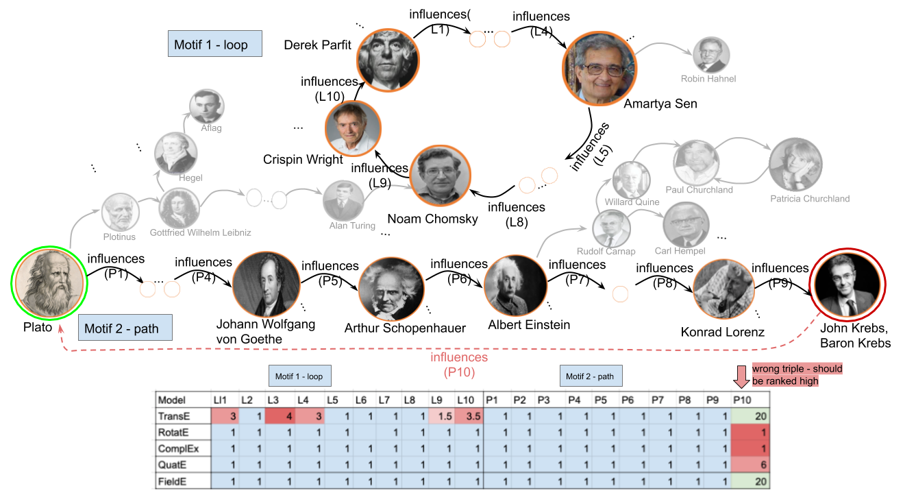
In this way, the major encoding capabilities of KGEs remain focused in the triple level. Therefore, capturing collective knowledge both from the structural and semantical aspects for groups of triples (sungraphs) stays dependent on the inherited characteristics from the underlying geometries. Within each geometry, the mathematical operations used in the score function make individual differences in encoding capability of KGEs. In most of the KGEs, while mapping each triple into a geometric space, naturally the subgraphs are also mapped. However, the extent to which the structure of subgraphs are preserved, remains limited to the characteristics of the considered geometric space, specially when a subgraph form complex and heterogeneous structures and motifs (i.e. statistically significant shapes distributed in the graph). Major part of the state-of-the-art KGEs (Zhang et al., 2019a; Sun et al., 2019; Trouillon et al., 2016; Bordes et al., 2013a) are designed in flat geometries which do not intrinsically support structural preservation. Consequently, the returned scores of certain triples involved in such heterogeneous structures are measured inaccurately. Such heterogeneous structures are not only possible to occur between nodes connected with multiple relations but also can be caused by a single relation. While many KGE models have been proposed, very few work have investigated on KGEs for discovery and encoding of heterogeneous subgraphs and motifs. Here, we focus on the case of complex motifs in multirelational graphs that are caused by one single relation e.g., “follows”, or “influences”. The nature of these relations leads to heterogeneous and completely different shapes in subgraphs, which is a prevailing case in many KGs. In Figure 2, we illustrate two possible subgraphs with different motifs generated by “influences” relation on the YAGO knowledge graph. The first subgraph is captured as a loop structure which is constructed by 10 nodes. The second subgraph forms a path structure which is created by the same relation among another set of 10 nodes.

Let us explore the following link prediction task by RotatE model on a toy KG with such motifs. The assumption is that, the RotatE model returns wrong inferences when two subgraphs are structured in different shapes with a same relation. To show this let us represent the above motifs as $m_{L}$ and $m_{P}$ – each with a set of 10 connected nodes ($e_{1}\dots e_{10}$) with one relation ($r$). Therefore, (${e_{1}}^{m_{L}}\dots e_{10}^{m_{L}}$) represents the nodes of motif ($m_{L}$) where they form a loop, and (${e_{1}}^{m_{P}}\dots e_{10}^{m_{P}}$) correspond to the nodes of another subgraph with the same relation but forming a path. For each triple in this graph e.g. (${e_{i}}^{m_{k}},r,{e_{j}}^{m_{k}}$), $k\in\{L,P\}$, the vector representation using RotatE is $\boldsymbol{e_{i}}^{m_{k}}\circ r\approx\boldsymbol{e_{j}}^{m_{k}}$. A complete representation of the motifs are then as following:

$$m_{L}:\begin{cases}({e_{1}}^{m_{L}},r,{e_{2}}^{m_{L}}),\rightarrow\boldsymbol{e_{1}}^{m_{L}}\circ r\approx\boldsymbol{e_{2}}^{m_{L}},\\ ({e_{2}}^{m_{L}},r,{e_{3}}^{m_{L}}),\rightarrow\boldsymbol{e_{2}}^{m_{L}}\circ r\approx\boldsymbol{e_{3}}^{m_{L}},\\ \vdots\\ ({e_{9}}^{m_{L}},r,{e_{10}}^{m_{L}}),\rightarrow\boldsymbol{e_{9}}^{m_{L}}\circ r\approx\boldsymbol{e_{10}}^{m_{L}},\\ ({e_{10}}^{m_{L}},r,{e_{1}}^{m_{L}}).\rightarrow\boldsymbol{e_{10}}^{m_{L}}\circ r\approx\boldsymbol{e_{1}}^{m_{L}}.\end{cases}$$

$$m_{P}:\begin{cases}({e_{1}}^{m_{P}},r,{e_{2}}^{m_{P}}),\rightarrow\boldsymbol{e_{1}}^{m_{P}}\circ r\approx\boldsymbol{e_{2}}^{m_{P}},\\ ({e_{2}}^{m_{2}},r,{e_{3}}^{m_{P}}),\rightarrow\boldsymbol{e_{2}}^{m_{P}}\circ r\approx\boldsymbol{e_{3}}^{m_{P}},\\ \vdots\\ ({e_{9}}^{m_{P}},r,{e_{10}}^{m_{P}}).\rightarrow\boldsymbol{e_{9}}^{m_{P}}\circ r\approx\boldsymbol{e_{10}}^{m_{P}}.\end{cases}$$

In order to compute the value of relation $r$, we start with the loop structure, by replacing the corresponding vectors of each triple in the following (e.g., by replacing the left side of $\boldsymbol{e_{2}}$ in the second triple equation of $m_{L}$, we get $\boldsymbol{e_{1}}^{m_{L}}\circ r\circ r=\boldsymbol{e_{3}}^{m_{L}}$). By doing this to the end, we conclude that $\boldsymbol{e_{1}}^{m_{L}}\circ r\dots\circ r=\boldsymbol{e_{1}}^{m_{L}}$ which means $r\circ\dots\circ r=1$ where $r$ is a complex number, therefore $\theta_{r}=\frac{2\pi}{10}$. This value is consistent for $r$ in the whole graph, therefore, this can be used to check whether the second motif is preserved. Here we replace the vectors as above and additionally include the value of $r$ driven from the first calculation. After some derivations, we have $\boldsymbol{e_{1}}^{m_{P}}*e^{\frac{20\pi i}{10}}=\boldsymbol{e_{10}}^{m_{P}}*r$. With a simplification steps, this results in $\boldsymbol{e_{1}}^{m_{P}}=\boldsymbol{e_{10}}^{m_{P}}*r$, from which the model infers that the triple (${e_{10}}^{m_{P}},r,{e_{1}}^{m_{P}}$) is positive. However, the actual shape of this motif is a path and this wrong inference shows a loop structure.

The root cause of this problem lies in the entity-dependent nature of this relation. However, most of the KGE models such as RotatE (as well as TransE, ComplEx, QuatE) consider relations independent of entities. This is visible in the heat map illustration in Figure 2. As shown, $P_{10}$ is a wrong triple and should be ideally ranked as high as possible. All the models except TransE do not preserve the path structure and provide a low rank for this triple (infer it as a correct triple). Although TransE preserves the path structure (ranking $P_{10}$ low), it fails in preserving the loop structure as it infers five triples to be wrong ($L_{1}$, $L_{3}$, $L_{4}$, $L_{9}$, and $L_{10}$). This is due to the limitation of their geometry.

In order to tackle this problem, our novel KGE models dubbed FieldE employs DEs for embedding of KGs into a vector space. Differential Equations (DEs) are used as powerful tools with a general framework to accurately define connection between neighboring points laid on trajectories, implying the continuity of changes, and consequently describing the underlying geometry. This is specially important because the success of a KGE model depends on the way it correctly specifies the underlying geometry that describes the natural proximity of data samples in a geometric space (Mathieu and Nickel, 2020). Designing FieldE with a well-specified geometry a) improves generalization, b) increases the interpretability. First-order Ordinary Differential Equations (FO-ODEs) are special class of DEs which represents a vector field on a smooth Riemannian manifold. Therefore, we particularly focus on FO-ODEs in designing our model. FieldE brings the power of DEs, embeddings and Neural Networks together and provides a fully comprehensive model capable of learning different motifs in subgraphs of a KG.

2. Related Work

Here, we collected prior work on the capability of embedding models in preserving subgraph structures, and semantically relational patterns. We also discuss the related work about the motifs and the use of DEs for different encoding purposes.

Learning Relational Motifs. The primary generation of embedding models includes a list of translation-based approaches where the encoding of motifs have only been discussed with the essence simple relational patterns such as 1-1 in TransE (Bordes et al., 2013b) and 1-many, many-1, and many-many in its follow up models (Ji et al., 2015; Lin et al., 2015; Wang et al., 2014). RotatE (Sun et al., 2019) is the first KGE model where rotational transformations have been used for encoding of more complex patterns such as symmetry, transitive, composition, reflexive, and inversion which also create complex subgraphs. Another group of KGEs which are using element-wise multiplication of transformed head and tail namely DisMult (Yang et al., 2015), ComplEx (Trouillon et al., 2016), QuatE (Zhang et al., 2019b), and RESCAL (Nickel et al., 2011), also belong to rotation-based models and some use the angle of transformed head and tail for measuring the correctness of the predicted links. Apart from some partial discussions about the capability of the models in encoding of relational patterns, capturing the motifs have not been directly targeted in any of these models. A recent KGE model named MuRP  (Balazevic et al., 2019) sheds the lights into the capability of embedding models in learning hierarchical relations. It proposes a geometrical approach for multi-relational graphs using Poincaré ball (Ji et al., 2016). However, our work not only covers hierarchical relations but also focuses on different complex motifs (e.g. simultaneous path and loop) constructed by one relation in multi-relational graphs. In (Suzuki et al., 2018), a very specific derivation of TransE model for encoding hierarchical relations have been proposed. The existing embedding models have been compared to the four different versions of the proposed Reimanian TransE namely hyperbolic, spherical, and euclidean geometries. Theses versions are designed for a very specific conditions in different geometries, while our model uses a neural network which generalizes cases beyond these.

Learning with Differential Equations. In (Chen et al., 2018), a family of deep neural network models has been proposed which parameterizes the derivative of a hidden state instead of the usual specification of a discrete sequence of hidden layers. In this approach, ODEs are used in the design of the continuous-depth networks with the purpose of providing an efficient computation of the network output which brings memory efficiency, adaptive computation, parameter efficiency, scalable and invertible normalizing flows, and continuous time-series models. It is applied for supervised learning on an image dataset, and time-series prediction. Few works use Lorenz model in their approaches (Bose et al., 2020; Chamberlain et al., 2017) which are not about knowledge graphs in our context.. This work used ODEs in the proposed approach without considering knowledge graphs and embeddings for link prediction tasks. In another recent work, the continuous normalizing flows have been extended for learning Riemannian manifolds (Mathieu and Nickel, 2020) in natural phenomena such as volcano eruptions. In this work, the manifold flows are introduced as solutions for ODEs which makes the defined neural network independent of the mapping requirements forced by the underlying euclidean space.

3. Preliminaries and Background

This section provides the preliminaries of the Riemannian Geometry and its corresponding key elements as the required background for our model. The aim of this paper is to embed nodes (entities) of a KG on trajectories of vector fields (relation) laid on the surface of a smooth Riemannian manifold. Therefore, we first provide the mathematical definitions (Franciscus, 2011) for manifold, and Tangent Space followed by introducing vector field including differential equations.

Manifold

A $d$-dimensional topological manifold denoted by $\mathcal{M}$ is a Hausdorff space with a countable base which is locally similar to a linear space. More precisely, $\mathcal{M}$ is locally homeomorphic to $\mathbb{R}^{d}$ where:

• For every point $p\in\mathcal{M}$, there is an open neighbourhood $U$ around $p$ and a homomorphism $\phi:U\xrightarrow[]{}V$ which maps $U$ to $V\subset\mathbb{R}^{d}.$ $\phi$ is called chart or the coordinate system. $\phi(p)\in\mathbb{R}^{d}$ is the image of $p\in U$, which is called the coordinates of $p$ in the chart.

• Let $\bigcup\limits_{i=1}^{n}U_{i}=\mathcal{M},\,\,\,i=1,\ldots,n,$ meaning that $\mathcal{M}$ is partitioned into $n$ parts denoted by $U_{i},i=1,\ldots,n.$ The set $\mathcal{P}=\{\phi_{i}|i=1,\ldots,n\},$ with domain $U_{i}$ for each $\phi_{i}$, is called atlas of $\mathcal{M}.$

Tangent Space

If we assume a particle as a moving object on a manifold $\mathcal{M}$, then at each point $p\in\mathcal{M}$, the particle is free to move in various directions with velocity $v$. The set of all the possible directions that a particle goes by passing point $p$ form a space called the Tangent space. Formally, given a point $p$ on a manifold $\mathcal{M}$, the tangent space $\mathcal{T}_{p}\mathcal{M}$ is the set of all the vectors which are tangent to all the curves, passing through point $p$. Let $\gamma:t\xrightarrow[]{}\mathcal{M}$ be a parametric curve on the manifold. $\gamma(t)$ maps $t\in[a,b]$ to $\mathcal{M}$ and passes through point $p$. A curve in the local coordinate is $\phi\circ\gamma:t\xrightarrow[]{}\mathbb{R}^{d}$, from $t$ to manifold and then to the local coordinate $x=\phi\circ\gamma(t)=\phi(\gamma(t))$. $x$ represents the position of a particle on the local coordinate and the rate of the changes for different positions (velocity) on point $p$ is computed by

(1) $$v=\frac{d\phi\circ\gamma(t)}{dt}|_{t=t_{0}}=\big{[}\frac{dx^{1}}{dt},\ldots,\frac{dx^{d}}{dt}\big{]}|_{t=t_{0}},$$

where $p=\gamma(t_{0}),x^{i}(t)$ is i-th component of the curve on the local coordinates. The tangent vector $v$ is velocity at point $p$ in the local coordinate. If we specify every possible curve passing $p$, then all of the velocity vectors form a set called tangent space. In other words, the tangent space represents all possible directions in which one can tangentially pass through $p$. In order to move in a direction with the shortest path, exponential map is used. The exponential map at point $p\in\mathcal{M}$ is denoted by $exp_{p}:\mathcal{T}_{p}\mathcal{M}\xrightarrow[]{}\mathcal{M}$. For a given small $\epsilon$ and $v\in\mathcal{T}_{p}\mathcal{M}$, the map $exp_{p}(\epsilon v)$ shows how a particle moves on $\mathcal{M}$ through the shortest path from $p$ with initial direction $v$ in $\mathbb{R}^{d}.$ A first order approximation of exponential map is given by $exp_{p}(v)=p+v$.

Riemannian Manifold

A tuple $(\mathcal{M},g)$ represents a Reimanian manifold where $\mathcal{M}$ is a real smooth manifold with a Riemannian metric $g$. The function $g_{p}=g(p)=\langle.,.\rangle_{p}:\mathcal{T}_{p}\mathcal{M}\times\mathcal{T}_{p}\mathcal{M}\xrightarrow[]{}\mathbb{R},p\in\mathcal{M}$ defines an inner product on the associated tangent space. The metric tensor is used to measure angle, length of curves, surface area and volume locally, and from which global quantities can be derived by integration of local contribution.

Vector Field

Let $x(t)$ be a temporal evolution of a trajectory on a $d$-dimensional smooth Riemannian manifold $\mathcal{M}$ and $\mathcal{T}\mathcal{M}=\bigcup\limits_{z\in\mathcal{M}}\mathcal{T}_{z}\mathcal{M}$ be a tangent bundle (the set of all tangent spaces on a Manifold). For a given Ordinary Differential Equation (ODE)

(2) $$\frac{dx(t)}{dt}=f_{\theta}(x(t)),$$

$f_{\theta}:\mathcal{M}\xrightarrow[]{}\mathcal{T}\mathcal{M}$ is a vector field on the manifold, which shows the direction and the speed of movements along which the trajectory evolves on the manifold’s surface.

The vector field defines the underlying dynamics of a trajectory on a manifold and can get various shapes with different sparsity/density as well as various flows with different degrees of rotation. In field theory, this is formalized by two concepts of Divergence and Curl. Divergence describes the density of the outgoing flow of a vector field from an infinitesimal volume around a given point $p$ on the manifold, while a Curl represents the infinitesimal rotation of a vector field around the point. Here we present the formal definition of Divergence and Curl. Without loss of generality, let $\boldsymbol{F}=f_{\theta_{x}}i+f_{\theta_{y}}j+f_{\theta_{z}}k$ be a continuously differentiable vector field in the Cartesian coordinates. The divergence of $\boldsymbol{F}$ is defined as follows

(3) $$\begin{split}div\boldsymbol{F}=\bigtriangledown.\boldsymbol{F}=(\frac{\partial}{\partial x},\frac{\partial}{\partial y},\frac{\partial}{\partial z}).(f_{\theta_{x}},f_{\theta_{y}},f_{\theta_{z}})\\ =\frac{\partial f_{\theta_{x}}}{\partial x}i+\frac{\partial f_{\theta_{y}}}{\partial y}j+\frac{\partial f_{\theta_{z}}}{\partial z}k.\end{split}$$

At a given point $p\in\mathcal{M},$ if $div\boldsymbol{F}(p)>0$, then the point is a source, i.e. the outflow on the point is more than the inflow. Conversely, if $div\boldsymbol{F}(p)<0$, then the point $p$ is sink i.e. the inflow on the point is more than the outflow. Given a continuous differentiable vector field $\boldsymbol{F}=f_{\theta_{x}}i+f_{\theta_{y}}j+f_{\theta_{z}}k$, a curl of the vector field is computed as following

(4) $$\begin{split}&curl\boldsymbol{F}=\bigtriangledown\times\boldsymbol{F}=\left|{\begin{array}[]{*{20}c}i&j&k\\ \frac{\partial}{\partial x}&\frac{\partial}{\partial y}&\frac{\partial}{\partial z}\\ f_{\theta_{x}}&f_{\theta_{y}}&f_{\theta_{z}}\\ &\end{array}}\right|=\\ &(\frac{\partial f_{\theta_{z}}}{\partial y}-\frac{\partial f_{\theta_{y}}}{\partial z})i+(\frac{\partial f_{\theta_{x}}}{\partial z}-\frac{\partial f_{\theta_{z}}}{\partial x})j+(\frac{\partial f_{\theta_{y}}}{\partial x}-\frac{\partial f_{\theta_{x}}}{\partial y})k.\end{split}$$

The curl is a vector with a limited length and a direction. The length of the vector shows the extent to which the vector field rotates and its direction specifies if the rotation is clock-wise or counterclockwise around the vector using right-hand rule.

4. Method

Figure 2. The Architecture of FieldE Model. The input to FieldE model is a knowledge graph which is shown in the upper part. A path structure is highlighted in the graph representation. The vector representation part (lower part) illustrates a trajectory of an ODE on a manifold. Nodes of the path are sequentially embedded on the trajectory guided by a neural network.

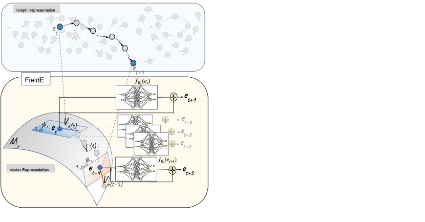
In this section, we propose FieldE, a new KGE model based on Ordinary Differential Equations (ODEs). The formulation of FieldE is presented in five folds: relation formulation, entity representation, triple representation, plausibility measurement, and vector field parameterization which are discussed in the remainder of this section.

Relation Formulation

FieldE represents each relation $r$ in a KG as a vector field ($f_{\theta_{r}}$) on a Riemannian manifold. $\theta_{r}$ denotes the parameters of the $f_{\theta_{r}}$ function and is constant by time. If we assume, $\boldsymbol{x}(t)$ is a parametric trajectory that evolves by the changes of parameter $t\in\mathbb{R}^{+}$, the following ODE can be defined per each relation of the KG:

(5) $$\frac{d\boldsymbol{x}(t)}{dt}=f_{\theta_{r}}(\boldsymbol{x}(t)),\,\,\,\boldsymbol{x}(t)\in\mathbb{R}^{d},$$

Given the above formulation, each relation of a KG forms a relation-specific geometric shape. This is consistent with the nature of KGs where different relations form different motifs and patterns in the graph.

Entity Representation

We represent each entity of a KG as a $d$-dimensional vector i.e. $\boldsymbol{e}\in\mathbb{R}^{d}$. The corresponding vectors are embedded on a trajectory of an ODE with an underlying relation-specific vector field. In other words, a sequence of entities (nodes) which are connected by a specific relation, are embedded sequentially through a trajectory laid on a relation-specific Riemannian surface.

Triple Learning

In order to formulate the steps for learning triples by FieldE, let $e_{t}$ and $e_{t+1}$ be the two subsequent nodes (entities shown in the upper part of the Figure 2) of a graph connected by a relation $r$. This actually forms as a triple $(e_{t},r,e_{t+1})$ in a directed graph for each sequentially connected entities with relation $r$. We consider $\boldsymbol{e}_{t},\boldsymbol{e}_{t+1}\in\mathbb{R}^{d}$ as the embedding vectors for the subsequent entities $e_{t}$ and $e_{t+1}$ (shown in the lower part of the Figure 2). Therefore, a triple in the vetor space can be modeled by time discretization (i.e. $\frac{d\boldsymbol{x}(t)}{dt}\approx\frac{\Delta\boldsymbol{x}}{\Delta t}=\frac{\boldsymbol{x}(t+1)-\boldsymbol{x}(t)}{1}=\boldsymbol{x}(t+1)-\boldsymbol{x}(t)$) over the equation 5 where $\boldsymbol{x}$ is replaced by entity embeddings ($\boldsymbol{e}$). This gives the following equation

(6) $$\Delta\boldsymbol{e}=\boldsymbol{e}(t+1)-\boldsymbol{e}(t)=f_{\theta_{r}}(\boldsymbol{e}(t)),$$

where the time step is set to 1 i.e. $\Delta t=1.$ This is the first order approximation of the exponential map where $\boldsymbol{e}(t+1)=exp_{\boldsymbol{e}(t)}(f_{\theta_{r}}(\boldsymbol{e}(t))$. Therefore, Equation 6 shows how to move on the trajectory of a relation-specific manifold $\mathcal{M}_{r}$ to take the shortest path from the node $e(t)$ with initial direction $f_{\theta_{r}}(\boldsymbol{e}(t))$. Note that the initial direction is dependent on the current node $e(t)$ and the relation $r$.

For a given positive triple $(e_{t},r,e_{t+1})$ in the graph, ($e(t)$ is shown by $e_{t}$ for simplicity from now onward), FieldE learns the triple by optimizing the embedding vectors i.e. $\boldsymbol{e}_{t},\boldsymbol{e}_{t+1}$ as well as the relation-specific vector field function parameters i.e. $\theta_{r}$ to fulfill

(7) $$\boldsymbol{e}_{t+1}\approx\boldsymbol{e}_{t}+v_{e_{t}},\,\,\,v_{e_{t}}=f_{\theta_{r}}(\boldsymbol{e}_{t}).$$

In order to regularize the current point $\boldsymbol{e}_{t}$ and the length of the step (velocity) $f_{\theta_{r}}(\boldsymbol{e}_{t})$, we propose the following formulation instead of the Equation 7. Therefore, for a positive triple $(\boldsymbol{e}_{t},r,\boldsymbol{e}_{t+1}),$ FieldE computes

(8) $$\boldsymbol{e}_{t+1}\approx\eta\boldsymbol{e}_{t}\,+\,(1-\eta)v_{e_{t}},\,\,\,v_{e_{t}}=f_{\theta_{r}}(\boldsymbol{e}_{t}),\eta\in[0,1].$$

Consequently, for a given negative triple $(\boldsymbol{e}^{\prime}_{t},r,\boldsymbol{e}^{\prime}_{t+1}),$ the following inequality should be fulfilled by FieldE

(9) $$\boldsymbol{e}^{\prime}_{t+1}\neq\eta\boldsymbol{e}^{\prime}_{t}+(1-\eta)v_{e_{t}},\,\,\,v_{e_{t}}=f_{\theta_{r}}(\boldsymbol{e}^{\prime}_{t}).$$

The Equations 8 and 9 are the optimal conditions to consider whether a triple is positive or negative. In the next part, we formulate the score function of FieldE to measure the degree to which a triple is plausible.

Plausibility Measurement

Given a triple $(e_{t},r,e_{t+1})$, the plausibility of the triple is measured by

(10) $$f_{r}(\boldsymbol{e}_{t},\boldsymbol{e}_{t+1})=-\|\boldsymbol{e}_{t+1}-\eta\boldsymbol{e}_{t}+(1-\eta)v_{e_{t}}\|,$$

for distance-based version of our model, DFieldE, and by

(11) $$f_{r}(\boldsymbol{e}_{t},\boldsymbol{e}_{t+1})=\langle\boldsymbol{e}_{t+1},\eta\boldsymbol{e}_{t}+(1-\eta)v_{e_{t}}\rangle,$$

for the semantic-matching version of our embedding model, SFieldE where $v_{e_{t}}=f_{\theta_{r}}(\boldsymbol{e}_{t})$.

Vector Field Parameterization

The selection of the function $f_{\theta_{r}}$ is important as it determines the shape of the manifold as well as the shape of the underlying vector field. In this paper, we propose two approaches for determining the vector field: a) we parameterize the vector field function $f_{\theta_{r}}$ by a neural network and propose a neuro-differential KGE models, b) we additionally propose linear version of our model where the vector field is modeled as a linear function. Here we explain the two steps in detail: Neuro-FieldE: Here we parameterize the vector field by a multi-layer feedforward neural network to approximate the underlying vector field

(12) $$f_{\theta_{r}}(\boldsymbol{e}_{t})=\sum w^{o}_{i}g(\sum w_{ij}^{L}g(\sum w_{jk}^{L-1}\ldots\sum w_{pq}^{2}g(w_{qz}^{1}\boldsymbol{e}_{t}+b_{z}^{1})),$$

where L is the number of hidden layer, $w^{o}$ denotes the output weight of the network and $w_{mn}^{l}$ is the weight connecting the $m$th node of the layer $l-1$ to the $n$th node of the $l$-th layer.

Parametrizing the vector field with a neural network gives the model enough flexibility to learn various shape vector fields (representing complex geometry) from complex data. This is due to the advantage neural networks which are universal approximators ((Hornik et al., 1989; Hornik, 1991; Nayyeri et al., 2017)) i.e. neural networks are capable of approximating any continuous function on a compact set. Linear-FieldE: Linear ODEs are a class of differential equations which have been widely used for several applications. Here we model the vector field as a linear function

(13) $$f_{\theta_{r}}(\boldsymbol{e}_{t})=\mathcal{A}_{r}\boldsymbol{e}_{t},$$

where $\mathcal{A}_{r}$ is a $d\times d$ matrix. Depending the eigenvalues of $\mathcal{A}_{r}$, the vector field gets various shapes. Below we present the theoretical analysis of FieldE and its advantage over other state-of-the-art KGE models.

4.1. Theoretical Analysis

In this part, we theoretically analyse the advantages of the core formulation of FieldE over other KGE models. We first show that while other existing models such as RotatE, ComplEx face issues while learning on single-relational complex motifs (such as having path and loop with a single relation), FieldE can easily model such complex structure. Moreover, we show that our model subsumes several popular existing KGEs and consequently inherits their capabilities in learning various well-studied patterns such as symmetry, inversion, etc.

Flexible Relation Embedding

Most of the existing state-of-the-art KGEs such as TransE, RotatE, QuatE, ComplEx etc., consider each relation of the KG as a constant vector to perform an algebraic operation such as translation or rotation. Therefore, the relation is entity-independent with regard to the applied algebraic operation. For example, TransE considers a relation as a constant vector to perform translations as

(14) $$\boldsymbol{e_{t}+r}\approx\boldsymbol{e_{t+1}}.$$

Therefore, a relation-specific transformation (here translation) is performed in the same direction with the same length, regardless of the different entities. This causes an issue on the learning outcome of complex motifs and patterns. To show this, let us consider a loop in a graph with a relation $r$ which connects three entities

(15) $$\begin{split}&\boldsymbol{e_{1}+r}\approx\boldsymbol{e}_{2},\\ &\boldsymbol{e_{2}+r}\approx\boldsymbol{e_{3}},\\ &\boldsymbol{e_{3}+r}\approx\boldsymbol{e_{1}}.\end{split}$$

After substituiting the first equation in the second one and comparing the result with the third equation, we conclude that $\boldsymbol{r}=\boldsymbol{0}$. This is indeed problematic because embedding of all the entities will be the same i.e. different entities are not distinguishable in the geometric space. Now we prove that our model can encode loop without marginal issues.

(16) $$\begin{split}&\boldsymbol{e_{1}+}f_{\theta_{r}}(e_{1})\approx\boldsymbol{e}_{2},\\ &\boldsymbol{e_{2}+}f_{\theta_{r}}(e_{2})\approx\boldsymbol{e_{3}},\\ &\boldsymbol{e_{3}+}f_{\theta_{r}}(e_{3})\approx\boldsymbol{e_{1}}.\end{split}$$

In FieldE, after substituiting the first equation in the second, and again substituting the result in the third equation, we obtain

(17) $$f_{\theta_{r}}(\boldsymbol{e}_{1})+f_{\theta_{r}}(\boldsymbol{e}_{2})+f_{\theta_{r}}(\boldsymbol{e}_{3})=\boldsymbol{0}.$$

The above equation can be satisfied by FieldE because neural networks with bounded continuous activation functions are universal approximators and universal classifiers (Hornik et al., 1989; Hornik, 1991; Nayyeri et al., 2017). Therefore, three points $\boldsymbol{e}_{1},\boldsymbol{e}_{2},\boldsymbol{e}_{3}$ can get the values by a well-specified neural network to hold the equality.

We additionally show that our model can also embed a path structure with other three entities $e_{4},e_{5},e_{6}$ while preserving a loop structure with $e_{1},e_{2},e_{3}.$

(18) $$\begin{split}&\boldsymbol{e_{4}+}f_{\theta_{r}}(\boldsymbol{e}_{4})\approx\boldsymbol{e}_{5},\\ &\boldsymbol{e_{5}+}f_{\theta_{r}}(\boldsymbol{e}_{5})\approx\boldsymbol{e_{6}},\\ &\boldsymbol{e_{6}+}f_{\theta_{r}}(\boldsymbol{e}_{6})\neq\boldsymbol{e_{4}}.\end{split}$$

After substituting the first equation in the second equation, and again substituting the results in the third equation, we have

(19) $$\begin{split}f_{\theta_{r}}(\boldsymbol{e}_{4})+f_{\theta_{r}}(\boldsymbol{e}_{5})+f_{\theta_{r}}(\boldsymbol{e}_{6})\neq\boldsymbol{0}.\end{split}$$

Because $\boldsymbol{e}_{1},\ldots,\boldsymbol{e}_{6}$ are distinct points in the domain of the function fulfilling Equations 17, and 19, there is a neural network that approximates these functions due to the universal approximation ability of the underlying network. Therefore, FieldE can learn two different sub-graph structures with the same relation.

The state-of-the-art KGE models like TransE, RotatE, ComplEx and QuatE are not capable of learning the above structure because they always model the initial direction of relation-specific movement. This is only to be dependent on the relation and ignore the role of entities in moving to the next node of the graph. Such limitation leads to wrong inferences when the graph contains complex motifs and patterns.

Subsumption Of Existing Models

Here, we prove that FieldE subsumes popular KGE models and consequently inherits their learning power.

Definition 4.1 (from (Kazemi and Poole, 2018)).

A model $M_{1}$ subsumes a model $M_{2}$ when any scoring over triples of a KG measured by model $M_{2}$ can also be obtained by model $M_{1}$.

Proposition 4.2.

DFieldE subsumes TransE and RotatE. SFieldE subsumes ComplEx and QuatE.

Because FieldE subsumes existing models, it consequently inherits their advantages in learning various patterns including symmetry, and anti-symmetry, transitivity, inversion and composition. Moreover, because ComplEx is fully expressive and it is subsumed by Neuro-SFieldE, we conclude that Neuro-SFieldE is also fully expressive. Beside modeling common patterns, FieldE is capable of learning more complex patterns and motifs such as having various motifs on a single relation e.g. having loop and path with one relation.

Proof.

Here we prove that DFieldE subsumes TransE. The FieldE assumption is

$$\boldsymbol{e}_{t+1}\approx\boldsymbol{e}_{t}+f_{\theta_{r}}(\boldsymbol{e}_{t}).$$

If we set $f_{\theta_{r}}=\boldsymbol{r}$ (constant vector field), then we have $\boldsymbol{e_{t+1}}\approx\boldsymbol{e}_{t}+\boldsymbol{r}$ which is the assumption of the TransE model for triple learning. ∎

Proof.

We now prove that DFieldE subsumes RotatE. The RotatE assumption is

(20) $$\boldsymbol{e}_{t+1}\approx\boldsymbol{e}_{t}\circ\boldsymbol{r},$$

where entities and relations are complex vectors and the modulus of each dimension of the relation vector is 1 i.e. $|\boldsymbol{r}|=1$. In the vector form, the equation 20 can be written in real (rotation) matrix-vector multiplication as following

$$\boldsymbol{e}_{t+1}^{v}\approx\boldsymbol{R}_{r}\boldsymbol{e}_{t}^{v},$$

where $\boldsymbol{R}_{r}$ is a rotation matrix and $\boldsymbol{e}_{t}^{v}$ represents the vector representation of complex numbers (with two components of real and imaginary). Given the assumption of DFieldE i.e.  $\boldsymbol{e}^{v}_{t+1}\approx\eta\boldsymbol{e}^{v}_{t}+(1-\eta)f_{\theta_{r}}(\boldsymbol{e}^{v}_{t}),$ and setting $\eta=0,$ and $f_{\theta_{r}}(\boldsymbol{e}_{t})=\boldsymbol{R}_{r}\boldsymbol{e}_{t}$, the assumption of RotatE is obtained. We conclude that, the RotatE model is a special case of DFieldE. ∎

Proof.

Here we present the proof of subsumption of ComplEx model. The SFieldE uses the following score function

$$f_{r}(\boldsymbol{e}^{v}_{t},\boldsymbol{e}^{v}_{t+1})=\langle\boldsymbol{e}^{v}_{t+1},\eta\boldsymbol{e}^{v}_{t}+(1-\eta)f_{\theta_{r}}(\boldsymbol{e}^{v}_{t})\rangle.$$

After setting $\eta=0,$ we have

(21) $$f_{r}(\boldsymbol{e}^{v}_{t},\boldsymbol{e}^{v}_{t+1})=\langle\boldsymbol{e}^{v}_{t+1},f_{\theta_{r}}(\boldsymbol{e}^{v}_{t})\rangle.$$

Now let us focus on the score function of ComplEx which is

(22) $$f_{r}(\boldsymbol{e}_{t},\boldsymbol{e}_{t+1})=Re(\langle\bar{\boldsymbol{e}}_{t+1},\boldsymbol{r},\boldsymbol{e}_{t}\rangle).$$

We represent the above equation in vectored version of complex numbers as following

(23) $$f_{r}(\boldsymbol{e}^{v}_{t},\boldsymbol{e}^{v}_{t+1})=\langle\boldsymbol{e}^{v}_{t+1},\alpha_{r}\boldsymbol{R}_{r}\boldsymbol{e}^{v}_{t}\rangle.$$

We can see if $f_{\theta_{r}}(\boldsymbol{e}_{t})=\alpha_{r}\boldsymbol{R}_{r}\boldsymbol{e}^{v}_{t}$ in Equation 21, we obtain the score of the ComplEx model in the vectorized in Equation 23. Therefore, ComplEx is also a special case of SFieldE.

∎

Proof.

Here we show that SFieldE subsumes QuatE. QuatE uses the following formulae for the score function

(24) $$f_{r}(\boldsymbol{e}_{t},\boldsymbol{e}_{t+1})=\boldsymbol{e}_{t+1}.\boldsymbol{r}\otimes\boldsymbol{e}_{t},$$

where $\otimes,.$ show the Hamilton product and element-wise product between two quaternion vectors. Similarly to RotatE, the Equation 24 can be written in matrix vector multiplication as follows

(25) $$f_{r}(\boldsymbol{e}^{v}_{t},\boldsymbol{e}^{v}_{t+1})=\langle\boldsymbol{e}^{v}_{t+1},\boldsymbol{R}_{r}\boldsymbol{e}^{v}_{t}\rangle,$$

where $\boldsymbol{R}_{r}$ is a $4d\times 4d$ matrix and $\boldsymbol{e}^{v}_{t}$ is a vectorized version of quaternion numbers.

Here, we show that the above equation can be constructed by the score function of SFieldE which is

$$f_{r}(\boldsymbol{e}^{v}_{t},\boldsymbol{e}^{v}_{t+1})=\langle\boldsymbol{e}^{v}_{t+1},\eta\boldsymbol{e}^{v}_{t}+(1-\eta)f_{\theta_{r}}(\boldsymbol{e}^{v}_{t})\rangle.$$

After setting $\eta=0,$ we have

(26) $$f_{r}(\boldsymbol{e}^{v}_{t},\boldsymbol{e}^{v}_{t+1})=\langle\boldsymbol{e}^{v}_{t+1},f_{\theta_{r}}(\boldsymbol{e}^{v}_{t})\rangle,$$

which will be same as the score function of QuatE in vectorized form if the vector Field is set to $f_{\theta_{r}}(\boldsymbol{e}^{v}_{t})=\boldsymbol{R}_{r}\boldsymbol{e}^{v}_{t}.$ Therefore, SFieldE subsumes QuatE model, as well. ∎

5. EXPERIMENTS AND RESULTS

In this section, we provide the results of evaluating FieldE ’s performance in comparison to already existing state-of-the-art embedding models. With a systematic analysis, we selected a list of KGEs to compare our model with, the list includes TransE, RotatE, TuckEr, ComplEx, QuatE, Dismult, ConvE, and MuRP.

5.1. Experimental Setup

Evaluation Metrics

We consider the standard metrics for compassion in KGEs namely Mean Reciprocal Rank (MRR), and Hits@n ($n=1,3,10$). MRR is measured by $\sum_{j=1}^{n_{t}}\frac{1}{r_{j}}$, where $r_{j}$ is the rank of the $j$-th test triple and $n_{t}$ - the number of triples in the test set. Hits@n is the number of testing triples which are ranked less than n, where n can be 1, 3, and 10.

Datasets

We run the experiments on two standard datasets namely FB15k-237 (Toutanova and Chen, 2015), and YAGO3-10 (Mahdisoltani et al., 2013). Statistics of these datasets including the number of their entities and relations as well as the split of train, test, and validation sets are shown in Table 1.

Table 1. Dataset Statistics. Number of entities and relations as well as the split of datasets.

Dataset	#Ent.	#Rel.	#Train	#Valid.	#Test
YAGO3-10	123k	37	1m	5k	5k
FB15k-237	15k	237	272k	20k	18k

Hyperparameter Search

We implemented our models in the Python using PyTorch library. We used Adam as the optimizer and tune the hyperparameters based on validation set. The learning rate ($r$) and batch size ($b$) are tuned on the set $r=\{0.0002,0.002,0.02,0,1\}$, $b=\{512,1024\}$ respectively. The embedding dimension $d$ is fixed to $100$ for YAGO3-10 and 1000 for FB15k-237. We set the number of negative sample to $100$ for B15K-237 and $500$ for YAGO3-10, and used adversarial negative sampling for our model as well as the other models we have re-implemented. We presented two versions of FieldE namely DFieldE and SFieldE. DfieldE uses distance function to compute the score of a triple (see equation 10). On the other SfieldE uses inner product for score computation 11. Each of the above version of FieldE can either used Neural Network to approximate the vector field or use an explicit linear function as a vector field. For the neural network based FieldE we add the prefix ”N” to the beginning of the name of our model (either NDFieldE or NSFieldE). For linear version of FieldE, we use ”L” as prefix in the name of the model (either LDFieldE or LSFieldE). For the Neural version of FieldE, we used a neural network with two hidden layers with $500,100$ hidden nodes for YAGO3-10 and $100,100$ for FB15K-237. We fixed the parameter $\eta$ to $1$ in equations 10 and 11. The details of the optimal hyperparameters are reported in the Table 2.

Table 2. The optimal parameter setting for FieldE is given for six different metrics.

Dataset	dimension.	learning rate.	batch size.	hidden nodes.	active function	neg.sample
YAGO3-10	100	0.002	512	(500,100)	tanh	500
FB15k-237	1000	0.1	1024	(100,100)	tanh	100

5.2. Results

The results are shown in Table 3 and the illustrations are depicted in Figure 3, and Figure 4. We first report the performance comparison of FieldE and other models. On both of the datasets, FieldE outperforms all the other models on all the metrics. On the FB15k-237 dataset, except MRR achieved equally by the Tucker model, all the other models fall short in comparison to FieldE. FieldE also outperform all the models in MRR on YAGO3-10.

Table 3. Link prediction results on d FB15k-237, and YAGO3-10. The highlight of performances for different models are marked.

Model	FB15k-237				YAGO3-10
	MRR	Hits@1	Hits@3	Hits@10	MRR	Hits@1	Hits@3	Hits@10
TransE	0.33	0.23	0.37	0.53	0.49	0.39	0.56	0.67
RotatE	0.34	0.24	0.37	0.53	0.49	0.40	0.55	0.67
TuckEr	0.36	0.26	0.39	0.54	-	-	-	-
ComplEx	0.32	-	-	0.51	0.36	0.26	0.40	0.55
QuatE	0.31	0.23	0.34	0.49	-	-	-	-
Dismult	0.24	0.15	0.26	0.42	0.34	0.24	0.28	0.54
ConvE	0.34	0.24	0.37	0.50	0.44	0.35	0.49	0.62
MuRP	0.34	0.25	0.37	0.52	0.35	0.25	0.40	0.57
FieldE	0.36	0.27	0.39	0.55	0.51	0.41	0.58	0.68

(a) some people influencing many (loop and path).

(b) few people influence many (source).

(c) dense influencing of many others (loop and path).

(d) many people influencing each other (loop)

(e) few people being influenced by many (sink).

(f) density in few people influencing others (source).

Figure 3. Illustration of different vector fields for the relation of “influences” from the YAGO3-10 dataset. The X and Y axis correspond to the 2D dimensions of vector fields.

(a) isconnectedto.

(b) isconnectedto.

(c) isconnectedto.

(d) hasGender

(e) hasGender.

(f) hasGender.

(g) owns

(h) owns.

(i) owns.

(j) livesIn

(k) livesIn.

(l) livesIn.

Figure 4. Illustration of vector fields learned for different relations.

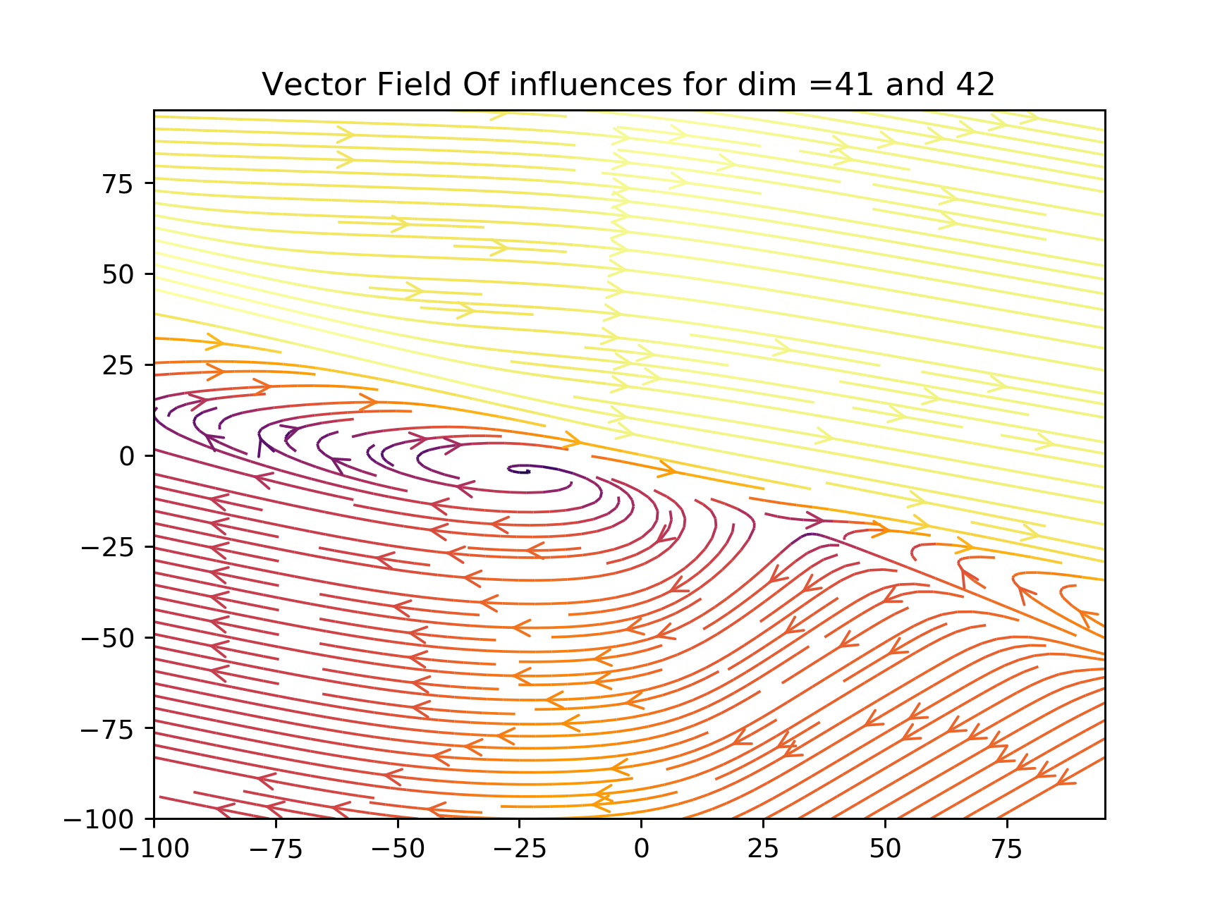
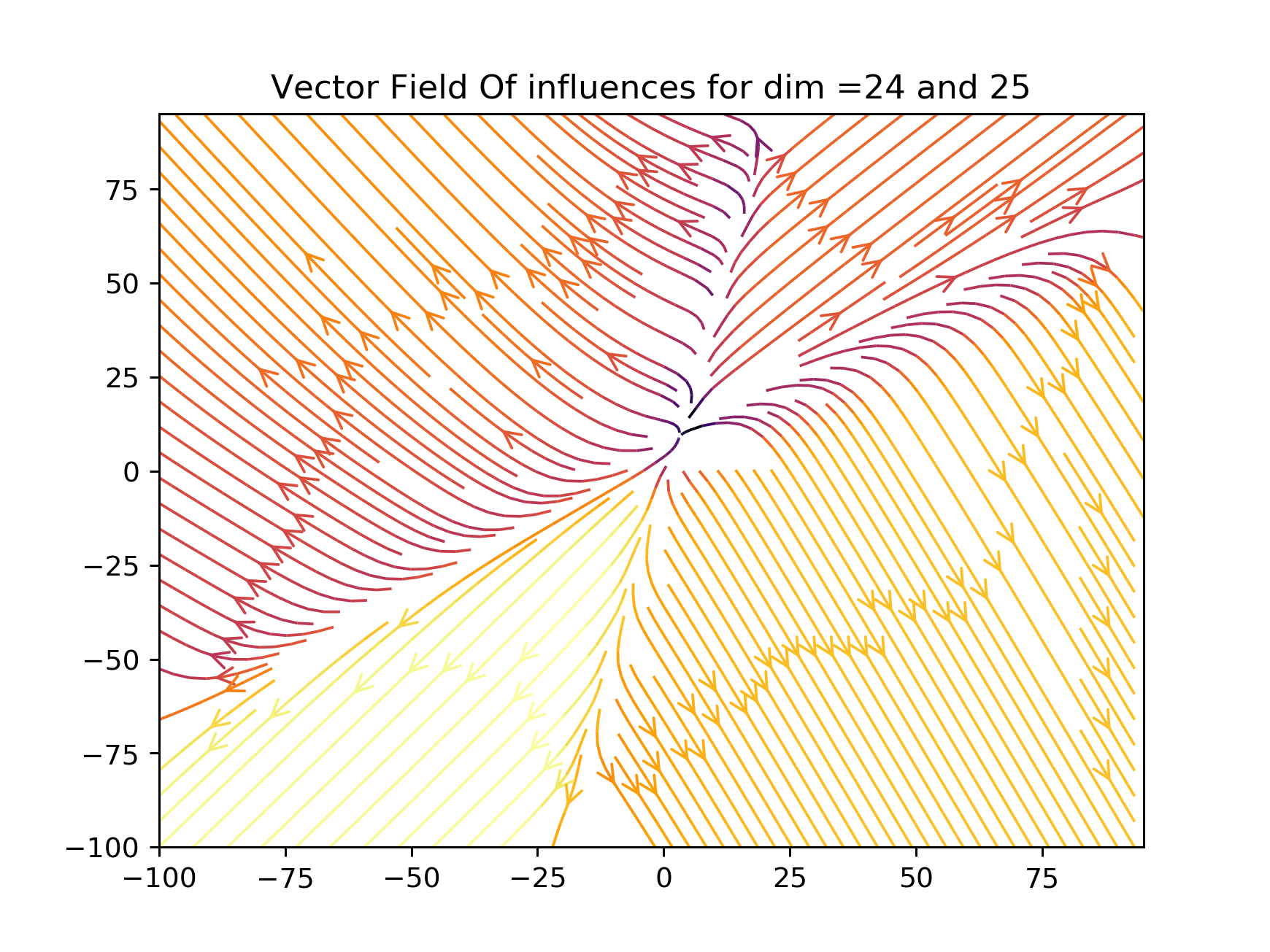
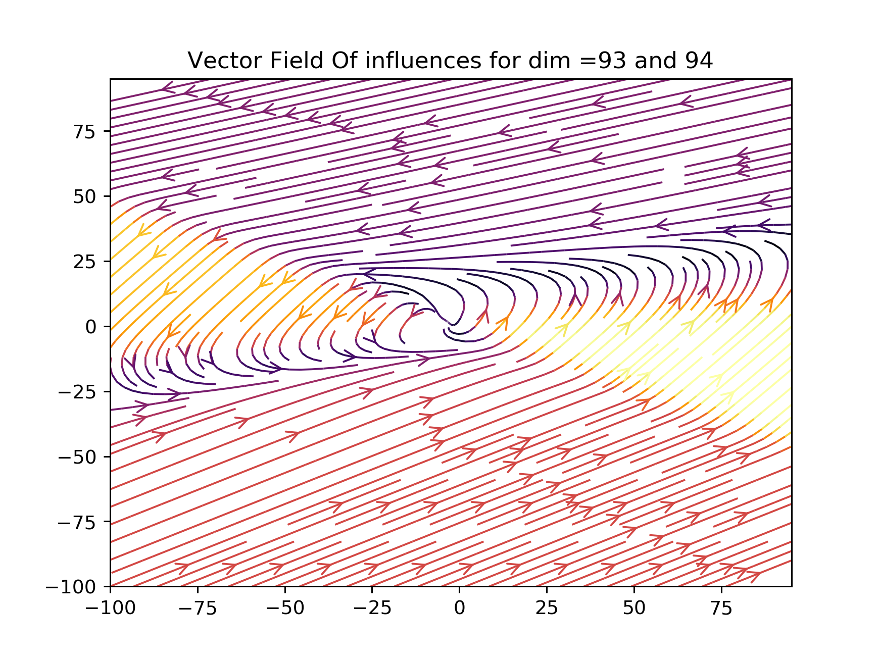
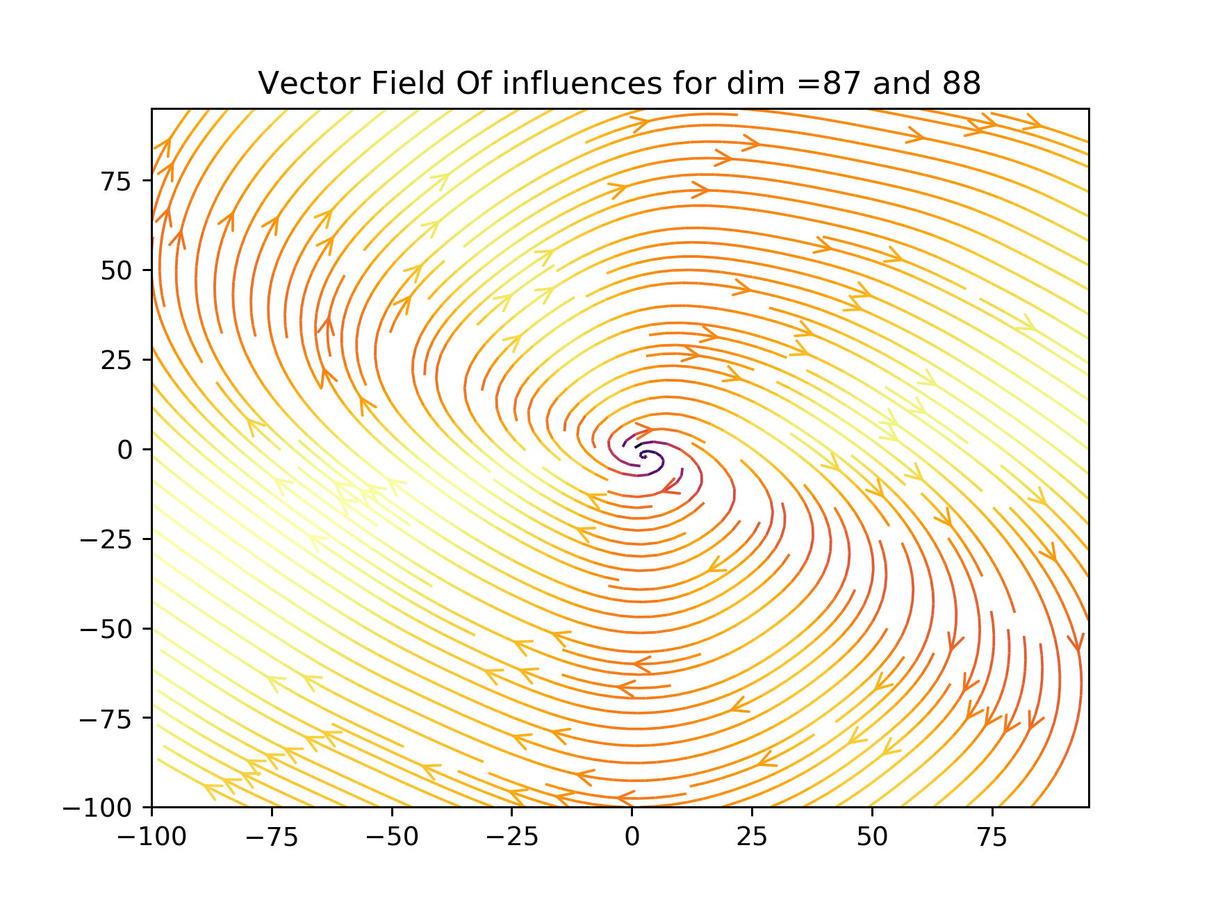
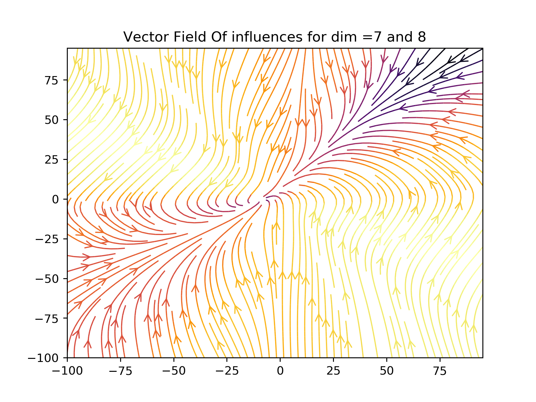
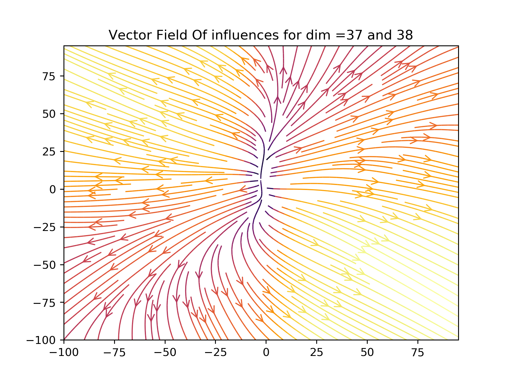
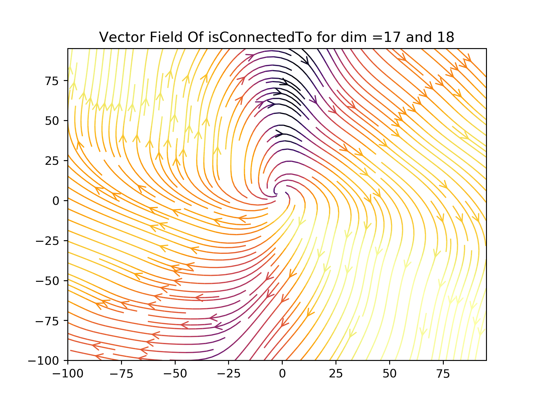
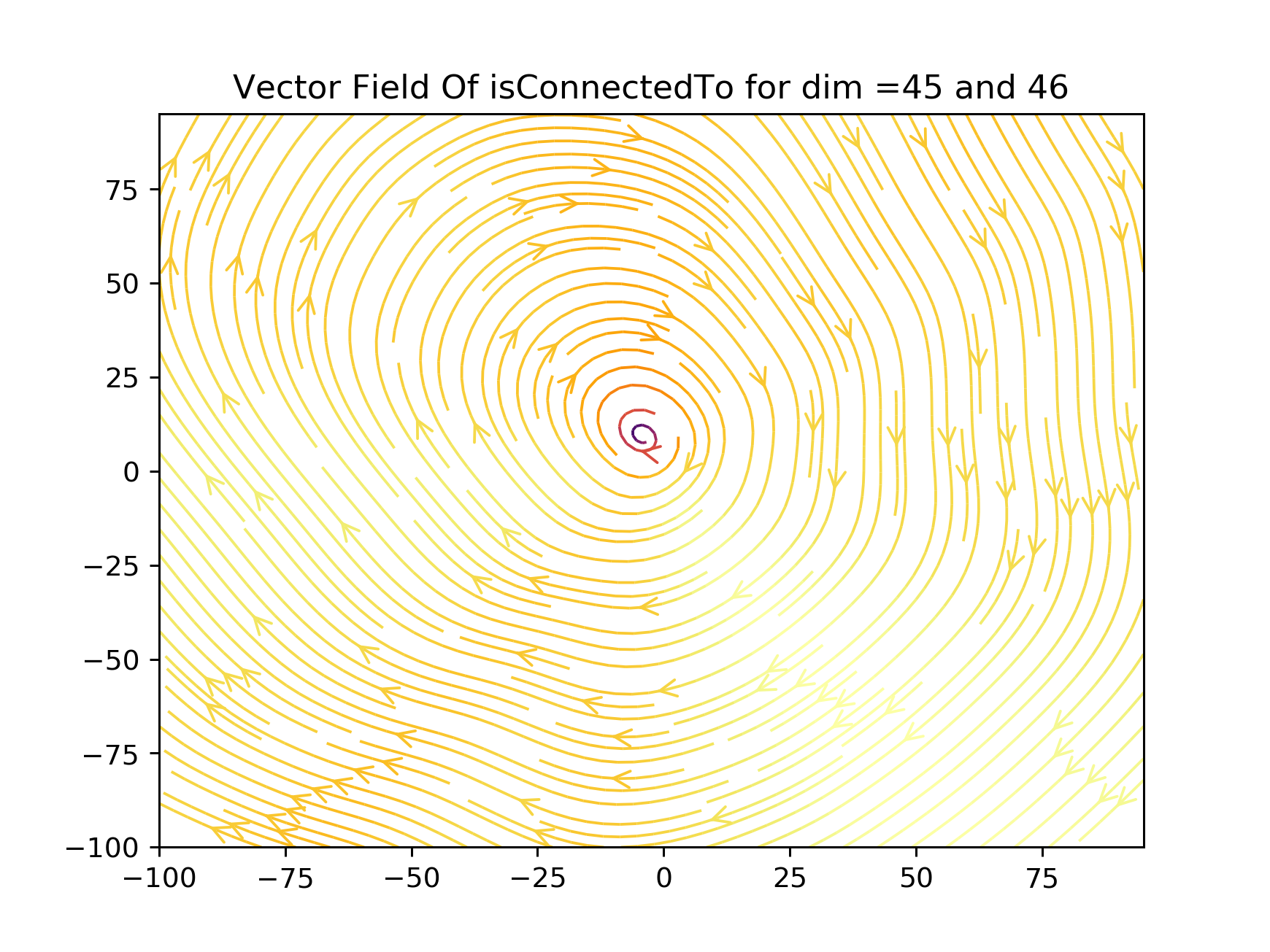
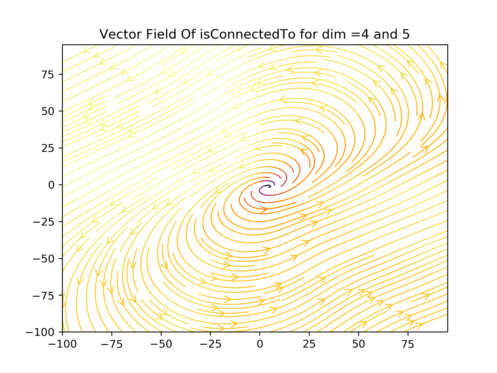
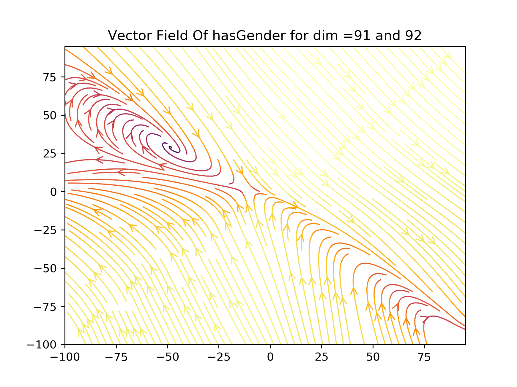
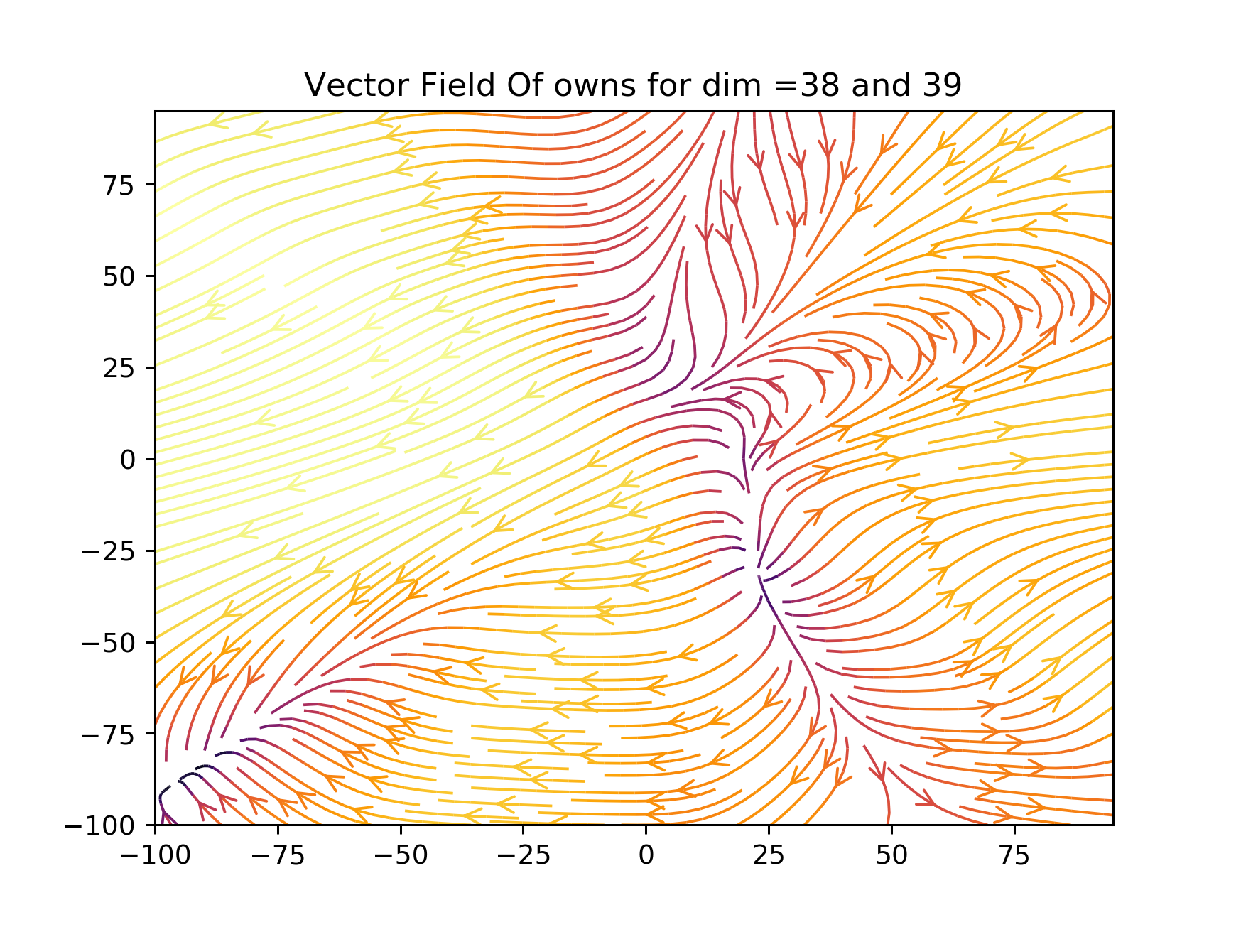
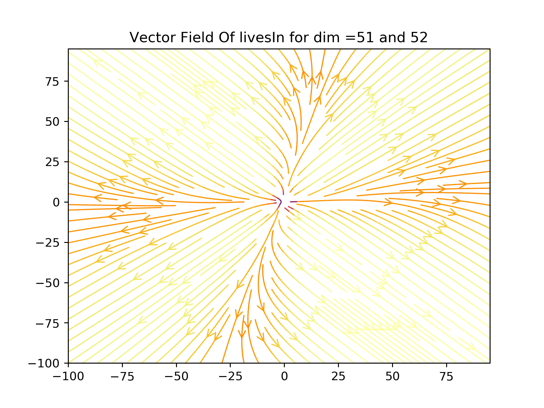
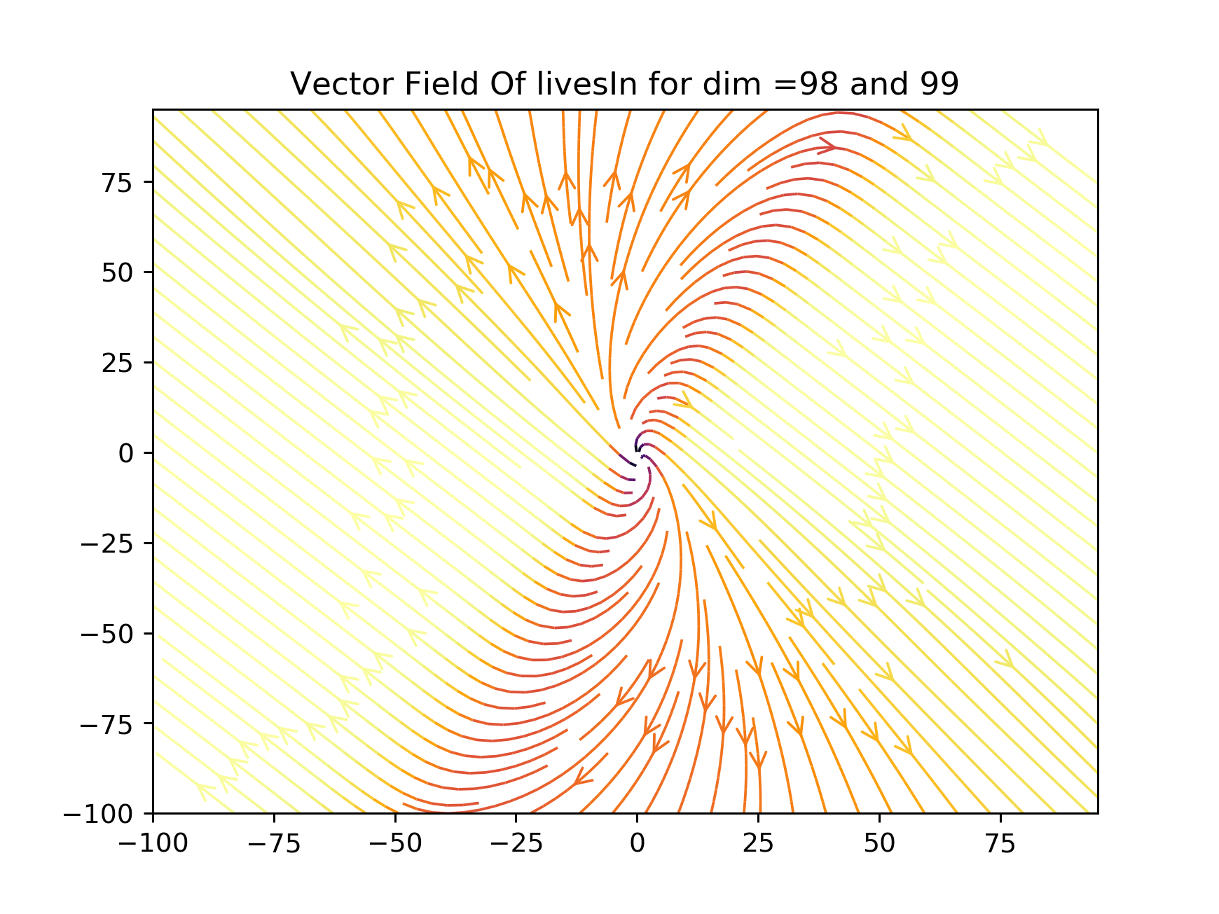
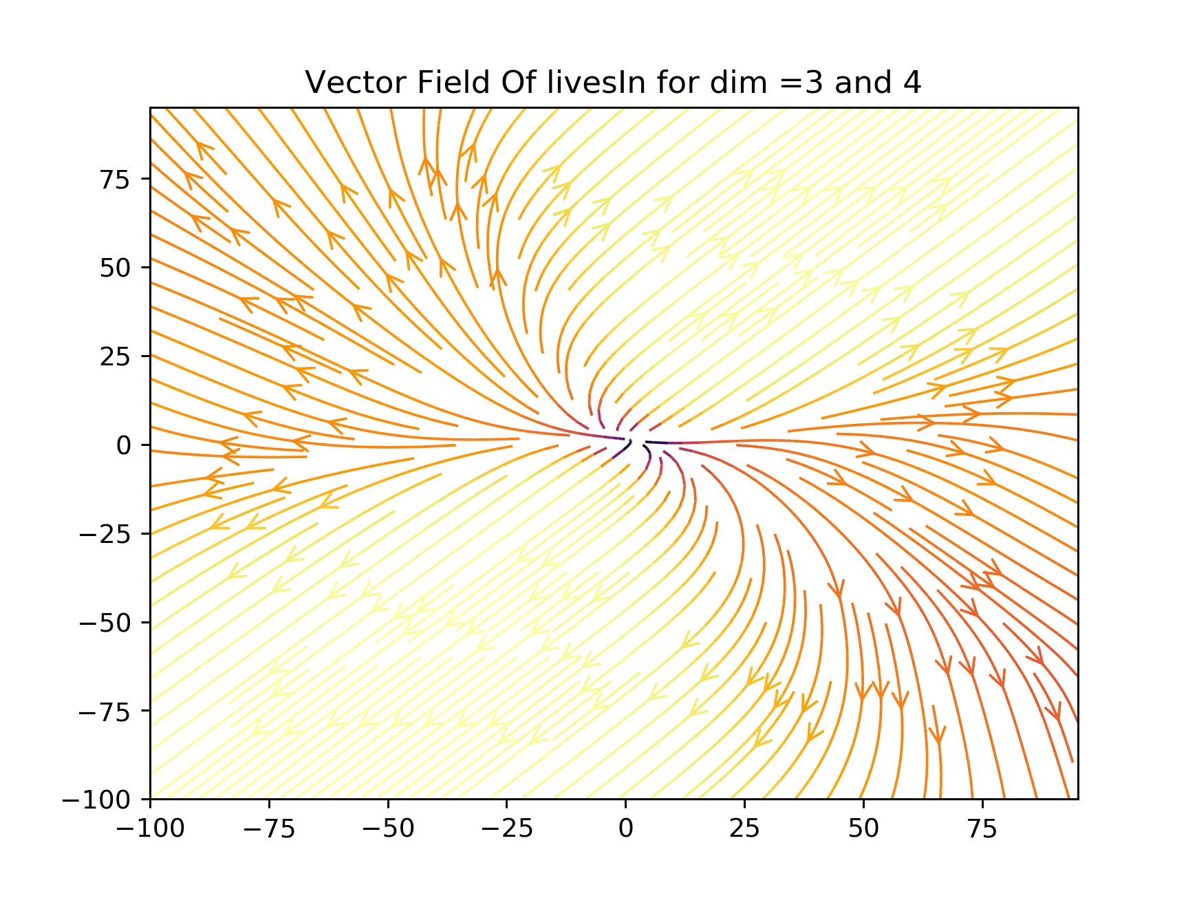
Following our motivating example which was focused with motifs created by the influences relation in the YAGO3-10 knowledge graph, we provide sample visualizations for vector fields of this relation in Figure 3. These visualizations have been selected among hundreds to only give an impression about the capability of FieldE model in motif learning. In order to provide a presentable illustration, we plot each vector fields in pair of dimensions. Therefore, for FieldE with $d=100$, we created $99$ pairs among which we selected six graphs constructed from dimension $\{(\boldsymbol{e}_{7},\boldsymbol{e}_{8}),(\boldsymbol{e}_{24},\boldsymbol{e}_{25}),(\boldsymbol{e}_{37},\boldsymbol{e}_{38}),(\boldsymbol{e}_{41},\boldsymbol{e}_{42}),(\boldsymbol{e}_{87},\boldsymbol{e}_{88}),(\boldsymbol{e}_{93},\boldsymbol{e}_{94})\}$.

In subfigure 3(a), the captured vector fields are shaping both as loop and path motifs simultaneously. It explains exactly the case illustrated in Figure 2 where some people are influencing others in a loop structure, and some people influence others in a path structure (without a return link). This shows a full structure preservation from the graph representation to the vector representation. As discussed before, this capability also avoids wrong inferences. Subgraph 3(b) shows trajectories of some people being a source influencer for many others. The subfigure 3(c) is another loop and path occurrence with more density.

A set of vector fields with a lot of loops is illustrated in subfigure 3(d). The interpretation of this vector field is that, there are a series of different people influencing each other in a loop structure with different number of entities. The subfigure 3(e) shows a set of sink nodes where they have been influenced by many. And finally, the subfigure 3(f) shows some more dense source entities. Overall, these illustrations double-prove the capability of FieldE inherited from ODEs and facilitated by the concept of vector field and trajectories.

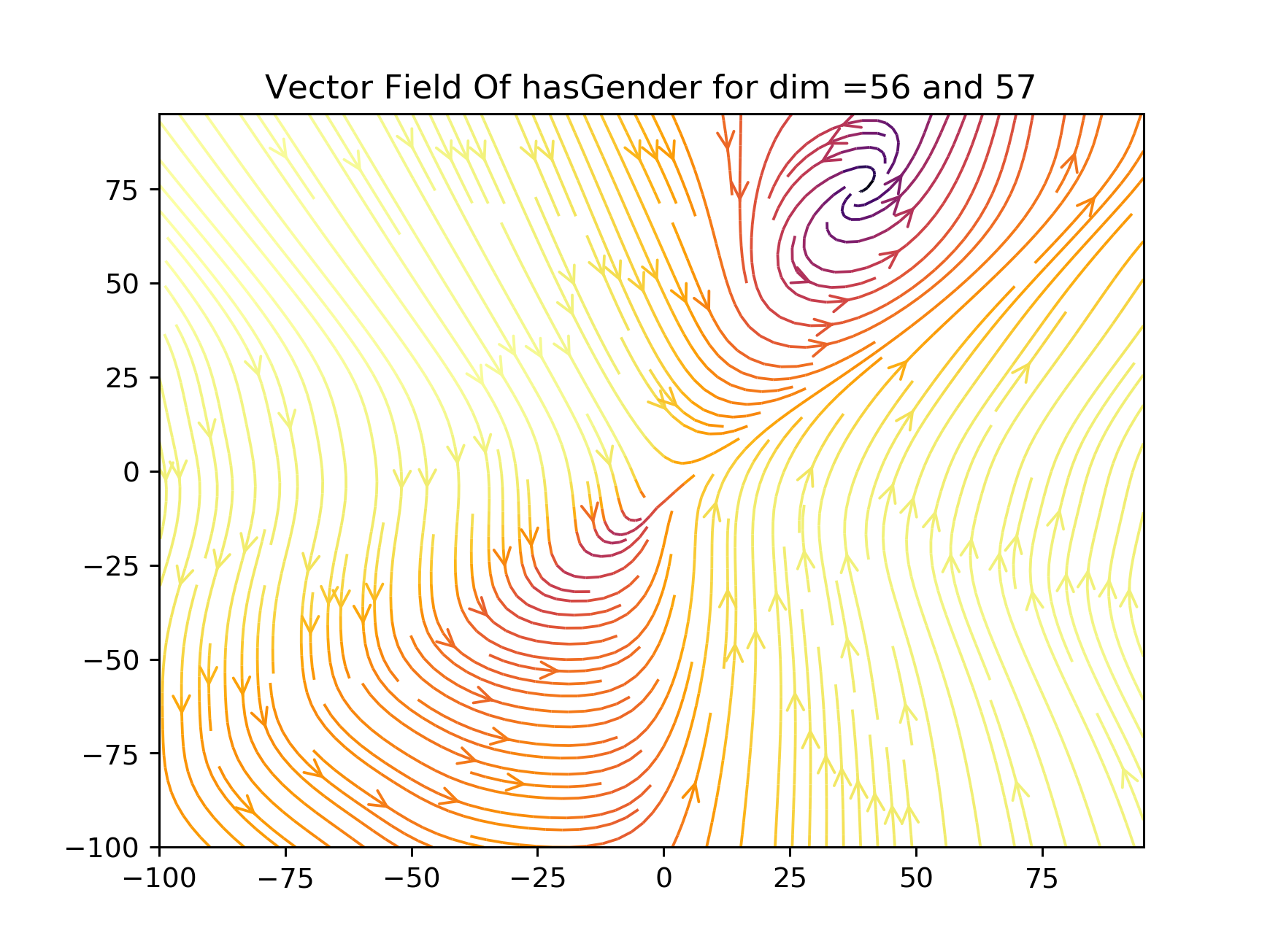
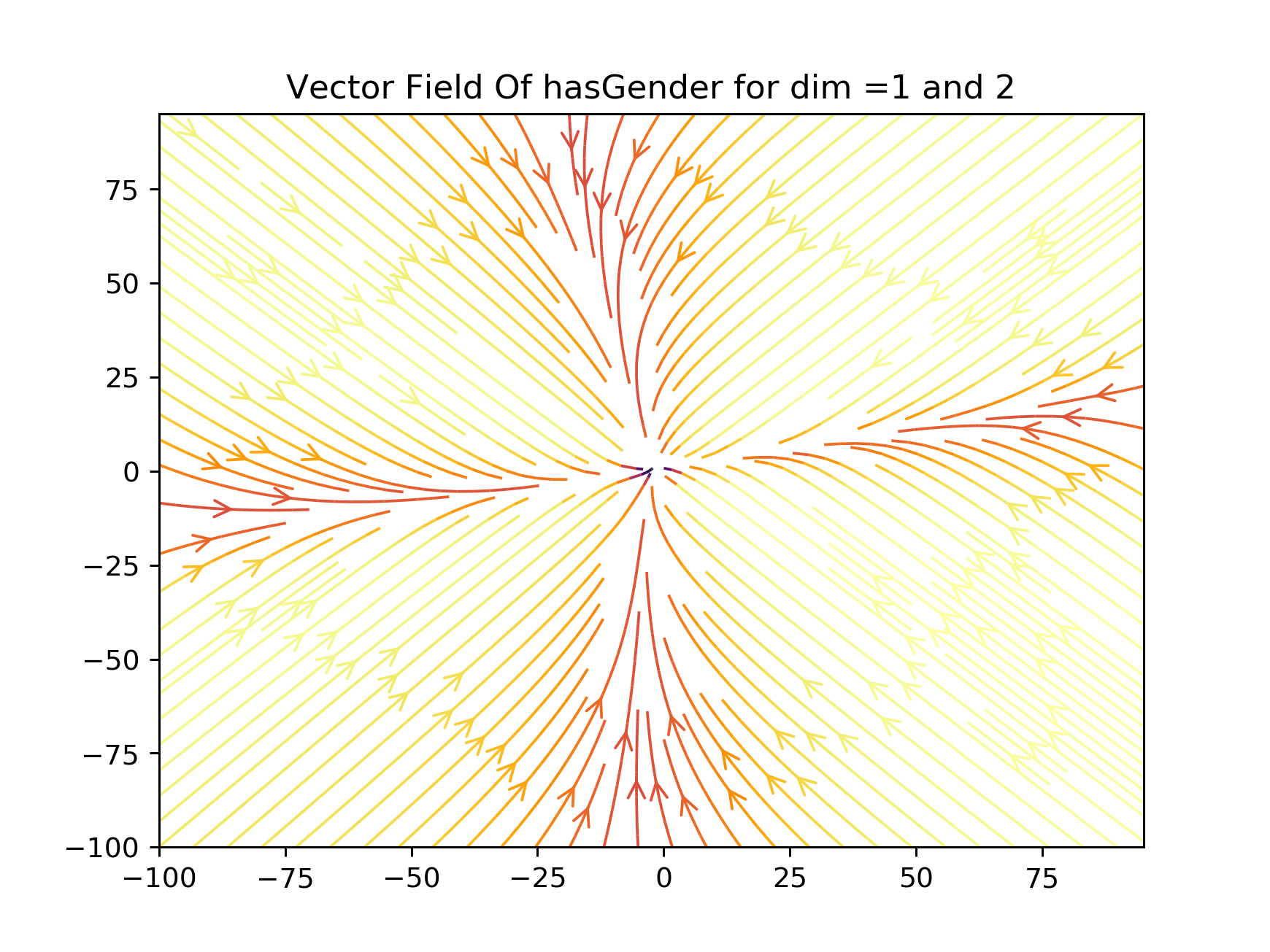
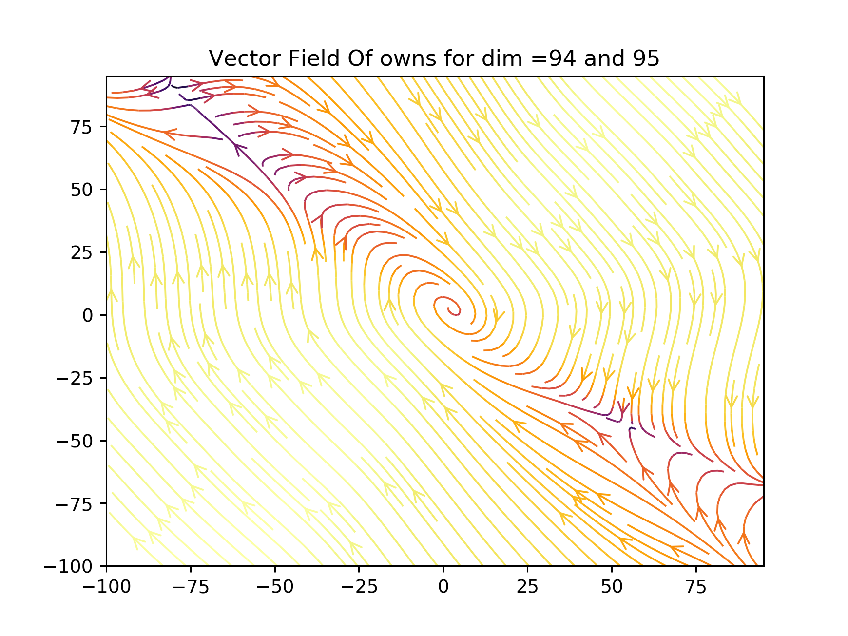
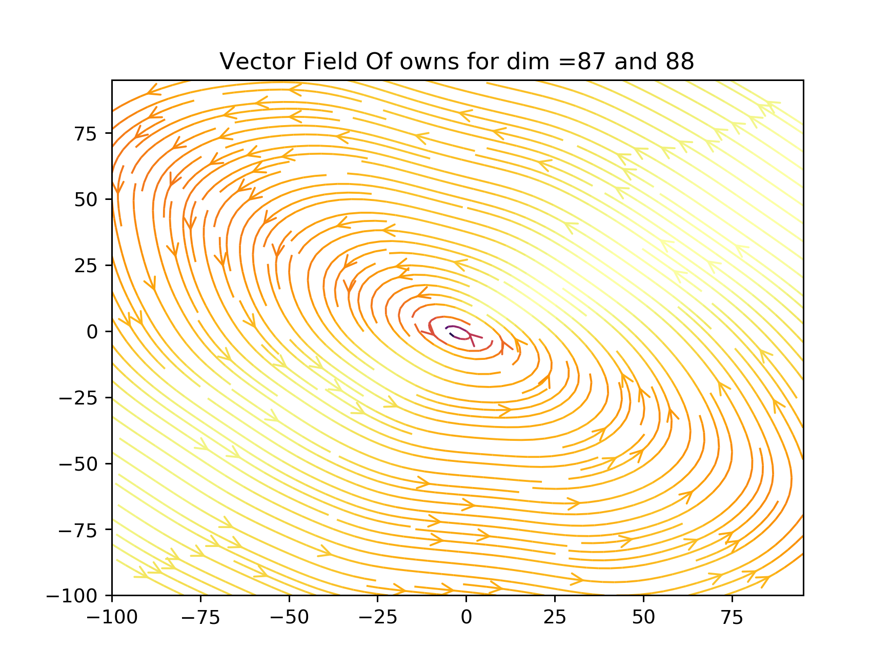
The visualizations in Figure 4 represent the subgraphs with different motifs including path and loop in different relations. Each row corresponds to the illustrations of one relation for which three different learned structures are selected to be shown. For example, subgraphs of 4(a), 4(b), and 4(c) correspond to the “isconnectedto” relation that shows which airports are connected to each other in different structures (loop and path). Our visualizations capture different learned motifs including path, and loop which show some airports are connected in a loop form and some not. In the subgraphs of 4(d), 4(e), 4(f), different motifs of “hasGender” relation are captured. Same for the “livesIn” relation, we show different illustrations of the vector fields in 4(j), 4(k), and 4(l). By all of these illustration, we aim at giving clarity on the effect of ODEs in learning vector fields which avoids wrong inferences. All of these are trajectories lain on relation-specific Reimanian manifold learned by the neural network of our model. The arrows shows the direction of motif evolution in the vector space for each shape.

6. Conclusion

This work presented a novel embedding models FieldE which is designed based on Ordinary Differential Equations. Since it inherits the characteristics of ODEs, it is capable of encoding different semantical and structural complexities in knowledge graphs. We modeled relations as vector fields on a Rimannian manifold and the entities of a knowledge graph which are connected through the considered relation, are taken as points on the trajectories laid on the manifold. We specifically parameterize the vector field by a neural network to learn the underlying geometry from the training graph. We examined FieldE on several datasets and compared it with a selection of best state-of-the-art embedding models. FieldE majorly outperforms all the models in all the metrics. We focused on showing the motif learning for loop and path simultaneously and preserving their structures from the graph representation to the vector representation. We showed that the neural network of FieldE learns various shapes of the vector fields and consequently the underlying geometry. In future versions of this, we plan to apply it on real world knowledge graph beside YAGO and FreeBase and further explore the effect of ODEs in learning process of knowledge graph embedding models.

References

- (1)
- Balazevic et al. (2019) Ivana Balazevic, Carl Allen, and Timothy Hospedales. 2019. Multi-relational Poincaré graph embeddings. In Advances in Neural Information Processing Systems. 4465–4475.
- Bordes et al. (2013a) Antoine Bordes, Nicolas Usunier, Alberto Garcia-Duran, Jason Weston, and Oksana Yakhnenko. 2013a. Translating embeddings for modeling multi-relational data. (2013), 2787–2795.
- Bordes et al. (2013b) Antoine Bordes, Nicolas Usunier, Alberto Garcia-Duran, Jason Weston, and Oksana Yakhnenko. 2013b. Translating embeddings for modeling multi-relational data. In Advances in neural information processing systems. 2787–2795.
- Bose et al. (2020) Avishek Joey Bose, Ariella Smofsky, Renjie Liao, Prakash Panangaden, and William L Hamilton. 2020. Latent Variable Modelling with Hyperbolic Normalizing Flows. arXiv preprint arXiv:2002.06336 (2020).
- Chamberlain et al. (2017) Benjamin Paul Chamberlain, James Clough, and Marc Peter Deisenroth. 2017. Neural embeddings of graphs in hyperbolic space. arXiv preprint arXiv:1705.10359 (2017).
- Chen et al. (2018) Ricky TQ Chen, Yulia Rubanova, Jesse Bettencourt, and David K Duvenaud. 2018. Neural ordinary differential equations. In Advances in neural information processing systems. 6571–6583.
- Franciscus (2011) M.J. Franciscus. 2011. Riemannian Geometry. International Book Market Service Limited. https://books.google.de/books?id=n6U_lwEACAAJ
- Hornik (1991) Kurt Hornik. 1991. Approximation capabilities of multilayer feedforward networks. Neural networks 4, 2 (1991), 251–257.
- Hornik et al. (1989) Kurt Hornik, Maxwell Stinchcombe, Halbert White, et al. 1989. Multilayer feedforward networks are universal approximators. Neural networks 2, 5 (1989), 359–366.
- Ji et al. (2015) Guoliang Ji, Shizhu He, Liheng Xu, Kang Liu, and Jun Zhao. 2015. Knowledge graph embedding via dynamic mapping matrix. In Proceedings of the 53rd Annual Meeting of the Association for Computational Linguistics and the 7th International Joint Conference on Natural Language Processing (Volume 1: Long Papers). 687–696.
- Ji et al. (2016) Guoliang Ji, Kang Liu, Shizhu He, and Jun Zhao. 2016. Knowledge graph completion with adaptive sparse transfer matrix. In Thirtieth AAAI conference on artificial intelligence.
- Kazemi and Poole (2018) Seyed Mehran Kazemi and David Poole. 2018. Simple embedding for link prediction in knowledge graphs. In Advances in neural information processing systems. 4284–4295.
- Lin et al. (2015) Yankai Lin, Zhiyuan Liu, Maosong Sun, Yang Liu, and Xuan Zhu. 2015. Learning entity and relation embeddings for knowledge graph completion. In Twenty-ninth AAAI conference on artificial intelligence.
- Mahdisoltani et al. (2013) Farzaneh Mahdisoltani, Joanna Biega, and Fabian M Suchanek. 2013. Yago3: A knowledge base from multilingual wikipedias.
- Mathieu and Nickel (2020) Emile Mathieu and Maximilian Nickel. 2020. Riemannian Continuous Normalizing Flows. arXiv preprint arXiv:2006.10605 (2020).
- Nayyeri et al. (2017) Mojtaba Nayyeri, Hadi Sadoghi Yazdi, Alaleh Maskooki, and Modjtaba Rouhani. 2017. Universal approximation by using the correntropy objective function. IEEE transactions on neural networks and learning systems 29, 9 (2017), 4515–4521.
- Nickel et al. (2011) Maximilian Nickel, Volker Tresp, and Hans-Peter Kriegel. 2011. A Three-Way Model for Collective Learning on Multi-Relational Data. 11 (2011), 809–816.
- Sun et al. (2019) Zhiqing Sun, Zhi-Hong Deng, Jian-Yun Nie, and Jian Tang. 2019. Rotate: Knowledge graph embedding by relational rotation in complex space. arXiv preprint arXiv:1902.10197 (2019).
- Suzuki et al. (2018) Atsushi Suzuki, Yosuke Enokida, and Kenji Yamanishi. 2018. Riemannian TransE: Multi-relational Graph Embedding in Non-Euclidean Space. (2018).
- Toutanova and Chen (2015) Kristina Toutanova and Danqi Chen. 2015. Observed versus latent features for knowledge base and text inference. In Proceedings of the 3rd Workshop on Continuous Vector Space Models and their Compositionality. 57–66.
- Trouillon et al. (2016) Théo Trouillon, Johannes Welbl, Sebastian Riedel, Éric Gaussier, and Guillaume Bouchard. 2016. Complex embeddings for simple link prediction. In International Conference on Machine Learning. 2071–2080.
- Wang et al. (2017) Quan Wang, Zhendong Mao, Bin Wang, and Li Guo. 2017. Knowledge graph embedding: A survey of approaches and applications. IEEE Transactions on Knowledge and Data Engineering 29, 12 (2017), 2724–2743.
- Wang et al. (2014) Zhen Wang, Jianwen Zhang, Jianlin Feng, and Zheng Chen. 2014. Knowledge graph embedding by translating on hyperplanes. In Twenty-Eighth AAAI conference on artificial intelligence.
- Yang et al. (2015) Bishan Yang, Wen-tau Yih, Xiaodong He, Jianfeng Gao, and Li Deng. 2015. Embedding entities and relations for learning and inference in knowledge bases. In Conference on Learning Representations (ICLR).
- Zhang et al. (2019a) Shuai Zhang, Yi Tay, Lina Yao, and Qi Liu. 2019a. Quaternion Knowledge Graph Embedding. arXiv preprint arXiv:1904.10281 (2019).
- Zhang et al. (2019b) Shuai Zhang, Yi Tay, Lina Yao, and Qi Liu. 2019b. Quaternion knowledge graph embeddings. In Advances in Neural Information Processing Systems. 2731–2741.