\newaliascnt

propthm\aliascntresettheprop \newaliascntcorothm\aliascntresetthecoro \newaliascntlemthm\aliascntresetthelem

Deep generative demixing: Recovering Lipschitz signals from noisy subgaussian mixtures

Aaron Berk University of British Columbia
Department of Mathematics
1984 Mathematics Rd., Vancouver, BC, Canada V6T 1Z2
Abstract

Generative neural networks (GNNs) have gained renown for efficaciously capturing intrinsic low-dimensional structure in natural images. Here, we investigate the subgaussian demixing problem for two Lipschitz signals, with GNN demixing as a special case. In demixing, one seeks identification of two signals given their sum and prior structural information. Here, we assume each signal lies in the range of a Lipschitz function, which includes many popular GNNs as a special case. We prove a sample complexity bound for nearly optimal recovery error that extends a recent result of Bora, et al. (2017) from the compressed sensing setting with gaussian matrices to demixing with subgaussian ones. Under a linear signal model in which the signals lie in convex sets, McCoy & Tropp (2014) have characterized the sample complexity for identification under subgaussian mixing. In the present setting, the signal structure need not be convex. For example, our result applies to a domain that is a non-convex union of convex cones. We support the efficacy of this demixing model with numerical simulations using trained GNNs, suggesting an algorithm that would be an interesting object of further theoretical study.

1 Introduction

Generative neural networks (GNNs) are neural networks that are capable of generating data from a learned distribution. Recently, GNNs have gained popularity for their performance on modelling spaces of natural images [5, 7, 6, 14, 25]. For example, variational autoencoders (VAEs) are composed of a “decoder” and “encoder” network, trained end-to-end to act as an approximate identity on the training distribution. The VAE learns a low-dimensional representation for elements within the data distribution [14] and its decoder is a type of GNN. For a thorough introduction to variational autoencoders, we recommend [5].

Recently, it was shown that some GNNs — including decoders from popular VAE architectures — could be used as structural proxies for generalized compressive sensing problems [1]. Roughly: it is possible to approximately recover a signal from a noisy underdetermined linear system with Gaussian measurements if the signal lies in the range of a Lipschitz function. The work specialized its recovery result from arbitrary Lipschitz functions, to the setting of Lipschitz-continuous neural networks. Many neural networks commonly used in practice are Lipschitz, supporting the relevance of this work to practical settings. For example, see [1, Lemma 4.2].

Several extensions of this work have been examined. In [30], the authors derive an improved sample complexity for compressed sensing-type problems when the underlying signal structure is the range of a ReLU neural network. Another version of this problem has been studied in which the measurements derive from a heavy-tailed, possibly corrupted distribution [11]. A further generalization studies the semi-parametrized single index model with possibly unknown possibly nonlinear link function, and in which the measurement vectors derive from a differentiable probability density function [30]. To our knowledge, a theoretical analysis of the demixing problem for two Lipschitz functions remains open.

The demixing problem refers to the identification of two unknown signals from their sum and given information about their structure. Sharp recovery bounds for convex demixing problems have been thoroughly investigated in [20], where the source signals are each assumed to be well encoded by some convex set. There, the authors show, under an incoherence condition, that recovery error depends on the effective dimension of the cones that govern the complexity of the source signals. Demixing with possibly unknown, possibly nonlinear link functions has been examined [27, 26]; however, the error bounds derived using this form of analysis may be coarse and difficult to analyze in practical settings [23].

The theory developed in [1] and [2] firmly lays the groundwork for the present work. Here, we investigate the demixing problem for two signals x,ysuperscript𝑥superscript𝑦x^{*},y^{*} that each lie in the range of an arbitrary Lipschitz function. We assume that xsuperscript𝑥x^{*} and ysuperscript𝑦y^{*} are combined by a subgaussian random mixing operation that we describe below, and seek approximate recovery of (x,y)superscript𝑥superscript𝑦(x^{*},y^{*}) with high probability on the mixing operation. The assumptions on the signal structure are mild, requiring only that each signal lie in the range of a Lipschitz function. These Lipschitz functions need not be the same, nor even have the same domain or range dimensions.

To specify, let G:kn:𝐺superscript𝑘superscript𝑛G:\mathbb{R}^{k}\to\mathbb{R}^{n} and H:km:𝐻superscriptsuperscript𝑘superscript𝑚H:\mathbb{R}^{k^{\prime}}\to\mathbb{R}^{m} be an LGsubscript𝐿𝐺L_{G}-Lipschitz and LHsubscript𝐿𝐻L_{H}-Lipschitz function. We will be concerned with the setting in which 1k<n<1𝑘𝑛1\leq k<n<\infty and 1k<m<1superscript𝑘𝑚1\leq k^{\prime}<m<\infty. We show that there are matrices Am×n𝐴superscript𝑚𝑛A\in\mathbb{R}^{m\times n} such that, if x:=G(u),y:=H(v)formulae-sequenceassignsuperscript𝑥𝐺superscript𝑢assignsuperscript𝑦𝐻superscript𝑣x^{*}:=G(u^{*}),y^{*}:=H(v^{*}) for points (u,v)k×ksuperscript𝑢superscript𝑣superscript𝑘superscriptsuperscript𝑘(u^{*},v^{*})\in\mathbb{R}^{k}\times\mathbb{R}^{k^{\prime}}, and

b=Ax+my+η𝑏𝐴superscript𝑥𝑚superscript𝑦𝜂\displaystyle b=Ax^{*}+\sqrt{m}y^{*}+\eta (1)

for some corruption ηm𝜂superscript𝑚\eta\in\mathbb{R}^{m}, then (x,y)superscript𝑥superscript𝑦(x^{*},y^{*}) may be approximated using only knowledge of (b,A,G,H)𝑏𝐴𝐺𝐻(b,A,G,H). Note the appearance of m𝑚\sqrt{m} in (1) is for normalization purposes only, due to the definition of A𝐴A below. The main result is stated in Theorem 1.

A key tool in the proof of our results is a modified restricted isometry property (RIP), first presented in [1]. There, the authors proved the condition holds with high probability for matrices with normal random entries. Here, we show that the condition holds with high probability for an expanded class of matrices: namely, matrices A𝐴A with independent isotropic subgaussian rows, as well as such concatenated matrices [IA]delimited-[]𝐼𝐴[I\,A], where I𝐼I is the identity matrix. Furthermore, we improve a result of [2] that establishes a deviation inequality for [IA]delimited-[]𝐼𝐴[I\,A]. We do this by improving the dependence on the subgaussian constant for A𝐴A in the deviation inequality, using an improved Bernstein’s inequality first proved in [12]. This improvement is stated in Theorem 2.

Finally, we support our theoretical results with numerical simulations presented in Numerics. There, we use two trained VAEs to solve a noiseless demixing problem. We visualize the recovery performance of our proposed algorithm, and plot apparent exponential convergence of the objective function vs. iteration number. We include a discussion that highlights potential topics of further interest for empirical investigations.

Motivation

The demixing problem can be viewed both as a tool for signal transmission, and as a tool for signal recovery. For example, the approach may be useful in the lossy transmission of two signals over a channel, where the sender and receiver possess the same Lipschitz continuous encoders G𝐺G and H𝐻H, and where the transmitted representation should use a small number of bits. In this scenario, the mixture may be amenable to further compression or encoding steps — such as that with error-correcting codes, or other sparsifying transforms [1, 19].

In [2], the expression (1) is used to describe the corrupted sensing model in which a ground truth signal xsuperscript𝑥x^{*}, after being encoded by A𝐴A, is corrupted by (possibly unknown) structured noise ysuperscript𝑦y^{*}, and unknown, unstructured noise η𝜂\eta. This interpretation translates to the present setting in the case where the structured noise process giving rise to ysuperscript𝑦y^{*} is well modelled by a Lipschitz function H𝐻H. Of interest to the present setting would be the case where either H𝐻H is a Lipschitz deep neural network that has been trained to model some noise process present in the corrupted measurements b𝑏b.

2 Background

We start by introducing the set-restriced eigenvalue condition that is critical to the results developed in [1] and the present work. This condition is the “modified RIP” hinted at above.

Definition ([1, Definition 1]).

Let Sn𝑆superscript𝑛S\subseteq\mathbb{R}^{n}. For some parameters γ>0,δ0formulae-sequence𝛾0𝛿0\gamma>0,\delta\geq 0, a matrix Am×n𝐴superscript𝑚𝑛A\in\mathbb{R}^{m\times n} is said to satisfy the SREC(S,γ,δ)SREC𝑆𝛾𝛿\operatorname{S-REC}(S,\gamma,\delta) if x1,x2Sfor-allsubscript𝑥1subscript𝑥2𝑆\forall x_{1},x_{2}\in S

A(x1x2)γx1x2δ.norm𝐴subscript𝑥1subscript𝑥2𝛾normsubscript𝑥1subscript𝑥2𝛿\displaystyle\left\|A\left(x_{1}-x_{2}\right)\right\|\geq\gamma\left\|x_{1}-x_{2}\right\|-\delta.

Next, we include for reference the relevant result of [1], which uses SRECSREC\operatorname{S-REC} for normal random matrices with iid entries to establish recovery bounds for compressed sensing (CS) with signals in the range of Lipschitz functions.

Theorem ([1, Theorem 1.2]).

Let G:kn:𝐺superscript𝑘superscript𝑛G:\mathbb{R}^{k}\rightarrow\mathbb{R}^{n} be an L𝐿L-Lipschitz function. Let Φm×NΦsuperscript𝑚𝑁\Phi\in\mathbb{R}^{m\times N} be a random Gaussian matrix for m=𝒪(klogLrδ)𝑚𝒪𝑘𝐿𝑟𝛿m=\mathcal{O}\left(k\log\frac{Lr}{\delta}\right), scaled so Φijiid𝒩(0,m1)subscriptΦ𝑖𝑗iidsimilar-to𝒩0superscript𝑚1\Phi_{ij}\overset{\text{iid}}{\sim}\mathcal{N}(0,m^{-1}). For any xNsuperscript𝑥superscript𝑁x^{*}\in\mathbb{R}^{N} and any observation b=Φx+η𝑏Φsuperscript𝑥𝜂b=\Phi x^{*}+\eta, let u^^𝑢\hat{u} minimize bΦG()2subscriptnorm𝑏Φ𝐺2\|b-\Phi G(\cdot)\|_{2} to within additive ε𝜀\varepsilon of the optimum over vectors with u^2rsubscriptnorm^𝑢2𝑟\|\hat{u}\|_{2}\leq r. Then, with probability 1exp(Ω(m))1Ω𝑚1-\exp(-\Omega(m)),

G(u^)x26minuku2rG(u)x2+3η2+2ε+2δ.subscriptnorm𝐺^𝑢superscript𝑥26subscriptFRACOP𝑢superscript𝑘subscriptnorm𝑢2𝑟subscriptnorm𝐺𝑢superscript𝑥23subscriptnorm𝜂22𝜀2𝛿\displaystyle\left\|G(\hat{u})-x^{*}\right\|_{2}\leq 6\min_{u\in\mathbb{R}^{k}\atop\left\|u\right\|_{2}\leq r}\left\|G(u)-x^{*}\right\|_{2}+3\|\eta\|_{2}+2\varepsilon+2\delta.

In extending  ([1, Theorem 1.2]). to the demixing setting (cfTheorem 1), we allow for a broader class of random matrices A𝐴A appearing in (1). To define this class of matrices, we start by defining a subgaussian random variable and subgaussian random vector.

Definition (Subgaussian).

For a random variable, X𝑋X, say X𝑋X is a subgaussian random variable with subgaussian norm bounded by K𝐾K, Xψ2Ksubscriptnorm𝑋subscript𝜓2𝐾\|X\|_{\psi_{2}}\leq K, if for some K>0𝐾0K>0,

(|X|t)2exp(t2/K2),for all t0.formulae-sequence𝑋𝑡2superscript𝑡2superscript𝐾2for all 𝑡0\displaystyle\mathbb{P}\left(|X|\geq t\right)\leq 2\exp\left(-t^{2}/K^{2}\right),\quad\text{for all }t\geq 0.

For a random vector Xnsuperscript𝑋superscript𝑛X^{\prime}\in\mathbb{R}^{n}, say X𝑋X is a subgaussian random vector with Xψ2Ksubscriptnormsuperscript𝑋subscript𝜓2𝐾\|X^{\prime}\|_{\psi_{2}}\leq K if

supe𝕊n1X,eψ2K.subscriptsupremum𝑒superscript𝕊𝑛1subscriptnorm𝑋𝑒subscript𝜓2𝐾\displaystyle\sup_{e\in\mathbb{S}^{n-1}}\|\langle X,e\rangle\|_{\psi_{2}}\leq K.

Additionally, we say that two random vectors X,Xn𝑋superscript𝑋superscript𝑛X,X^{\prime}\in\mathbb{R}^{n} are isotropic if 𝔼XXT=In𝔼superscript𝑋superscript𝑋𝑇subscript𝐼𝑛\operatorname*{\mathbb{E}}X^{\prime}X^{T}=I_{n}.

Definition (K𝐾K-subgaussian matrix).

If Am×n𝐴superscript𝑚𝑛A\in\mathbb{R}^{m\times n} is a matrix whose rows Ainsubscript𝐴𝑖superscript𝑛A_{i}\in\mathbb{R}^{n} are independent, isotropic subgaussian random vectors with norm at most K𝐾K, we call A𝐴A a K𝐾K-subgaussian matrix.

Two geometric objects of particular importance to CS problems are the Gaussian width and Gaussian complexity, which often appear in deviation inequalities used to control K𝐾K-subgaussian matrices on bounded sets.

Definition (Gaussian width/complexity).

Define the Gaussian width w(𝒯)w𝒯\operatorname{w}(\mathcal{T}) and Gaussian complexity γ(𝒯)𝛾𝒯\gamma(\mathcal{T}) of a set 𝒯n𝒯superscript𝑛\mathcal{T}\subseteq\mathbb{R}^{n} by

w(𝒯)w𝒯\displaystyle\operatorname{w}(\mathcal{T}) :=𝔼supx𝒯x,g,assignabsent𝔼subscriptsupremum𝑥𝒯𝑥𝑔\displaystyle:=\operatorname*{\mathbb{E}}\sup_{x\in\mathcal{T}}\langle x,g\rangle, γ(𝒯)𝛾𝒯\displaystyle\gamma(\mathcal{T}) :=𝔼supx𝒯|x,g|,assignabsent𝔼subscriptsupremum𝑥𝒯𝑥𝑔\displaystyle:=\operatorname*{\mathbb{E}}\sup_{x\in\mathcal{T}}|\langle x,g\rangle|, gisubscript𝑔𝑖\displaystyle g_{i} iid𝒩(0,1).iidsimilar-to𝒩01\displaystyle\overset{\text{iid}}{\sim}\mathcal{N}(0,1).

When A𝐴A is a K𝐾K-subgaussian matrix, we define B=B(A):=[AmI]𝐵𝐵𝐴assigndelimited-[]𝐴𝑚𝐼B=B(A):=\left[\begin{array}[]{rr}A&\sqrt{m}I\end{array}\right] to be the concatenation of A𝐴A with a scaled identity matrix (obtained by appending the columns of the second matrix to the first). We may alternately refer to B𝐵B or A𝐴A as the “subgaussian mixing matrix” or “mixing matrix”; it will be clear from context whether we mean B𝐵B or A𝐴A. To establish recovery bounds for the Lipschitz demixing problem with K𝐾K-subgaussian matrices, we use an improved version of the following deviation inequality for subgaussian mixing matrices B𝐵B.

Theorem ([2, Theorem 1]).

Let Am×n𝐴superscript𝑚𝑛A\in\mathbb{R}^{m\times n} be a K𝐾K-subgaussian matrix and 𝒯n×m𝒯superscript𝑛superscript𝑚\mathcal{T}\subseteq\mathbb{R}^{n}\times\mathbb{R}^{m} be bounded. Then

𝔼(x,y)𝒯|Ax+my2mx22+y22|CK2γ(𝒯)𝑥𝑦𝒯𝔼subscriptnorm𝐴𝑥𝑚𝑦2𝑚superscriptsubscriptnorm𝑥22superscriptsubscriptnorm𝑦22𝐶superscript𝐾2𝛾𝒯\displaystyle\underset{(x,y)\in\mathcal{T}}{\mathbb{E}}\left|\|Ax+\sqrt{m}y\|_{2}-\sqrt{m}\cdot\sqrt{\|x\|_{2}^{2}+\|y\|_{2}^{2}}\right|\leq CK^{2}\cdot\gamma(\mathcal{T})

For any t0𝑡0t\geq 0, the event

sup(x,y)𝒯|Ax+my2mx22+y22|CK2[γ(𝒯)+trad(𝒯)]subscriptsupremum𝑥𝑦𝒯subscriptnorm𝐴𝑥𝑚𝑦2𝑚superscriptsubscriptnorm𝑥22superscriptsubscriptnorm𝑦22𝐶superscript𝐾2delimited-[]𝛾𝒯𝑡rad𝒯\displaystyle\sup_{(x,y)\in\mathcal{T}}\left|\|Ax+\sqrt{m}y\|_{2}-\sqrt{m}\cdot\sqrt{\|x\|_{2}^{2}+\|y\|_{2}^{2}}\right|\leq CK^{2}[\gamma(\mathcal{T})+t\cdot\operatorname{rad}(\mathcal{T})]

holds with probability at least 1exp(t2)1superscript𝑡21-\exp\left(-t^{2}\right).

Above, rad(𝒯):=supx𝒯x2assignrad𝒯subscriptsupremum𝑥𝒯subscriptnorm𝑥2\operatorname{rad}(\mathcal{T}):=\sup_{x\in\mathcal{T}}\|x\|_{2} denotes the radius of the set 𝒯𝒯\mathcal{T}. Our improvement to this result, given in Theorem 2, is to establish an improved dependence on the subgaussian constant K𝐾K, from K2superscript𝐾2K^{2} to KlogK𝐾𝐾K\sqrt{\log{K}}.

Finally, we require  ([1, Lemma 4.3]). to connect the aforementioned pieces. It is worth noting that this lemma essentially requires no modification from its original statement for it to be applicable to the demixing problem.

Lemma ([1, Lemma 4.3]).

Let Am×n𝐴superscript𝑚𝑛A\in\mathbb{R}^{m\times n} be drawn from a distribution such that:

  1. 1.

    SREC(S,γ,δ)SREC𝑆𝛾𝛿\operatorname{S-REC}(S,\gamma,\delta) holds with probability 1p1𝑝1-p;

  2. 2.

    for every fixed xn,Ax22x2formulae-sequence𝑥superscript𝑛subscriptnorm𝐴𝑥22subscriptnorm𝑥2x\in\mathbb{R}^{n},\|Ax\|_{2}\leq 2\|x\|_{2} with probability 1p1𝑝1-p.

For any xnsuperscript𝑥superscript𝑛x^{*}\in\mathbb{R}^{n} and noise ηm𝜂superscript𝑚\eta\in\mathbb{R}^{m}, let y=Ax+η𝑦𝐴superscript𝑥𝜂y=Ax^{*}+\eta. Let x^^𝑥\hat{x} satisfy

yAx^2minxSyAx2+ϵ.subscriptnorm𝑦𝐴^𝑥2subscript𝑥𝑆subscriptnorm𝑦𝐴𝑥2italic-ϵ\displaystyle\|y-A\hat{x}\|_{2}\leq\min_{x\in S}\|y-Ax\|_{2}+\epsilon.

Then, with probability 12p12𝑝1-2p,

x^x2(4γ+1)minxSxx2+1γ(2η2+ϵ+δ).subscriptnorm^𝑥superscript𝑥24𝛾1subscript𝑥𝑆subscriptnormsuperscript𝑥𝑥21𝛾2subscriptnorm𝜂2italic-ϵ𝛿\displaystyle\left\|\hat{x}-x^{*}\right\|_{2}\leq\left(\tfrac{4}{\gamma}+1\right)\min_{x\in S}\left\|x^{*}-x\right\|_{2}+\tfrac{1}{\gamma}(2\|\eta\|_{2}+\epsilon+\delta).

As one final point regarding notation, we shall reserve the letters c,C>0𝑐𝐶0c,C>0 for absolute constants, whose value may change from one appearance to the next.

2.1 Two demixing modifications

Before moving on to the main results of this work, we discuss two modifications of the demixing problem (1), which trivially reduce to an application of ([1, Theorem 1.2])..

2.1.1 One mixing matrix

In the first modification, we assume that (x,y)superscript𝑥superscript𝑦(x^{*},y^{*}) are defined as in (1), and define instead b(1):=Φ(x+y)+ηassignsuperscript𝑏1Φsuperscript𝑥superscript𝑦𝜂b^{(1)}:=\Phi(x^{*}+y^{*})+\eta, where Φijiid𝒩(0,m1)subscriptΦ𝑖𝑗iidsimilar-to𝒩0superscript𝑚1\Phi_{ij}\overset{\text{iid}}{\sim}\mathcal{N}(0,m^{-1}) and ηm𝜂superscript𝑚\eta\in\mathbb{R}^{m} is some unknown fixed corruption. In this setting, we show that the two signals may be recovered but make no guarantee about correctly recovering each ground-truth signal.

For simplicity, assume k=k𝑘superscript𝑘k=k^{\prime}, LG=LH=Lsubscript𝐿𝐺subscript𝐿𝐻𝐿L_{G}=L_{H}=L and define w:=(u,v)2kassignsuperscript𝑤superscript𝑢superscript𝑣superscript2𝑘w^{*}:=(u^{*},v^{*})\in\mathbb{R}^{2k}. Similarly, write w:=(u,v)2kassign𝑤𝑢𝑣superscript2𝑘w:=(u,v)\in\mathbb{R}^{2k} and define the function F:2kn:𝐹superscript2𝑘superscript𝑛F:\mathbb{R}^{2k}\to\mathbb{R}^{n} by F(w):=G(u)+H(v)assign𝐹𝑤𝐺𝑢𝐻𝑣F(w):=G(u)+H(v) so that b(1):=ΦF(w)+ηmassignsuperscript𝑏1Φ𝐹superscript𝑤𝜂superscript𝑚b^{(1)}:=\Phi F(w^{*})+\eta\in\mathbb{R}^{m}. Using ([1, Theorem 1.2])., one may determine some w^2k^𝑤superscript2𝑘\hat{w}\in\mathbb{R}^{2k} that approximates wsuperscript𝑤w^{*} with high probability on the matrix ΦΦ\Phi.

Proposition \theprop.

Suppose mC2klog(2Lwδ)𝑚𝐶2𝑘2𝐿normsuperscript𝑤𝛿m\geq C\cdot 2k\log\left(\frac{2L\|w^{*}\|}{\delta}\right). Let w^:=(u^,v^)2kassign^𝑤^𝑢^𝑣superscript2𝑘\hat{w}:=(\hat{u},\hat{v})\in\mathbb{R}^{2k} minimize yΦF(w)2subscriptnorm𝑦Φ𝐹𝑤2\|y-\Phi F(w)\|_{2} within additive error ε>0𝜀0\varepsilon>0 over vectors w2k𝑤superscript2𝑘w\in\mathbb{R}^{2k} with wwnorm𝑤normsuperscript𝑤\|w\|\leq\|w^{*}\|. With probability at least 1exp(cm)1𝑐𝑚1-\exp(-cm),

F(w^)F(w)2=G(u^)G(u)+H(v^)H(v)23η2+2ε+2δsubscriptnorm𝐹^𝑤𝐹superscript𝑤2subscriptnorm𝐺^𝑢𝐺superscript𝑢𝐻^𝑣𝐻superscript𝑣23subscriptnorm𝜂22𝜀2𝛿\displaystyle\|F(\hat{w})-F(w^{*})\|_{2}=\|G(\hat{u})-G(u^{*})+H(\hat{v})-H(v^{*})\|_{2}\leq 3\|\eta\|_{2}+2\varepsilon+2\delta
Proof.

The proof is a consequence of  ([1, Theorem 1.2]).. Indeed, first notice that F𝐹F is 2L2𝐿\sqrt{2}L Lipschitz, because G𝐺G and H𝐻H are L𝐿L-Lipschitz:

F(w)F(w)2subscriptnorm𝐹𝑤𝐹superscript𝑤2\displaystyle\|F(w)-F(w^{\prime})\|_{2} G(u)G(u)+H(v)H(v)Luu+Lvvabsentnorm𝐺𝑢𝐺superscript𝑢norm𝐻𝑣𝐻superscript𝑣𝐿norm𝑢superscript𝑢𝐿norm𝑣superscript𝑣\displaystyle\leq\|G(u)-G(u^{\prime})\|+\|H(v)-H(v^{\prime})\|\leq L\|u-u^{\prime}\|+L\|v-v^{\prime}\|
2Luu2+vv2=2Lww2.absent2𝐿superscriptnorm𝑢superscript𝑢2superscriptnorm𝑣superscript𝑣22𝐿subscriptnorm𝑤superscript𝑤2\displaystyle\leq\sqrt{2}L\sqrt{\|u-u^{\prime}\|^{2}+\|v-v^{\prime}\|^{2}}=\sqrt{2}L\|w-w^{\prime}\|_{2}.

Next observe that F𝐹F is a d𝑑d-layer ReLU network because G𝐺G and H𝐻H are. Indeed, the linear transformations WiGki×ki1,WiHki×ki1formulae-sequencesuperscriptsubscript𝑊𝑖𝐺superscriptsubscript𝑘𝑖subscript𝑘𝑖1superscriptsubscript𝑊𝑖𝐻superscriptsuperscriptsubscript𝑘𝑖superscriptsubscript𝑘𝑖1W_{i}^{G}\in\mathbb{R}^{k_{i}\times k_{i-1}},W_{i}^{H}\in\mathbb{R}^{k_{i}^{\prime}\times k_{i-1}^{\prime}} used in defining G𝐺G and H𝐻H can, at each layer, be merged into block-diagonal transformations

Wi:=[WiG𝟎𝟎WiH](ki+ki)×(ki1+ki1),i1,,d.formulae-sequenceassignsubscript𝑊𝑖delimited-[]superscriptsubscript𝑊𝑖𝐺00superscriptsubscript𝑊𝑖𝐻superscriptsubscript𝑘𝑖superscriptsubscript𝑘𝑖subscript𝑘𝑖1superscriptsubscript𝑘𝑖1𝑖1𝑑\displaystyle W_{i}:=\left[\begin{array}[]{cc}W_{i}^{G}&\mathbf{0}\\ \mathbf{0}&W_{i}^{H}\end{array}\right]\in\mathbb{R}^{(k_{i}+k_{i}^{\prime})\times(k_{i-1}+k_{i-1}^{\prime})},i\in 1,\ldots,d.

to obtain

F(w)=[IdnIdn]σWdσWd1σW1(w).𝐹𝑤delimited-[]subscriptId𝑛subscriptId𝑛𝜎subscript𝑊𝑑𝜎subscript𝑊𝑑1𝜎subscript𝑊1𝑤\displaystyle F(w)=\left[\mathrm{Id}_{n}\,\mathrm{Id}_{n}\right]\circ\sigma\circ W_{d}\circ\sigma\circ W_{d-1}\circ\cdots\circ\sigma\circ W_{1}(w).

Applying  ([1, Theorem 1.2]). thereby completes the proof. ∎

2.2 Two mixing matrices

Alternately, one may assume that xsuperscript𝑥x^{*} and ysuperscript𝑦y^{*} are mixed as b(2):=Φ1x+Φ2y+ηassignsuperscript𝑏2subscriptΦ1superscript𝑥subscriptΦ2superscript𝑦𝜂b^{(2)}:=\Phi_{1}x^{*}+\Phi_{2}y^{*}+\eta, where Φi,i=1,2formulae-sequencesubscriptΦ𝑖𝑖12\Phi_{i},i=1,2 are independent and have the same distribution as ΦΦ\Phi above. Indeed, observe that b(2)superscript𝑏2b^{(2)} may be written as

b(2)superscript𝑏2\displaystyle b^{(2)} :=Φ¯[G(u)H(v)]+ηassignabsent¯Φdelimited-[]𝐺superscript𝑢𝐻superscript𝑣𝜂\displaystyle:=\overline{\Phi}\left[\begin{array}[]{r}G(u^{*})\\ H(v^{*})\end{array}\right]+\eta Φ¯¯Φ\displaystyle\overline{\Phi} :=[Φ1Φ2].assignabsentdelimited-[]subscriptΦ1subscriptΦ2\displaystyle:=\left[\begin{array}[]{rr}\Phi_{1}&\Phi_{2}\end{array}\right].

Since the concatentated matrix Φ¯¯Φ\overline{\Phi} has entries Φ¯ijiid𝒩(0,m1)subscript¯Φ𝑖𝑗iidsimilar-to𝒩0superscript𝑚1\overline{\Phi}_{ij}\overset{\text{iid}}{\sim}\mathcal{N}(0,m^{-1}), a similar line of reasoning as in One mixing matrix using F¯(w):=[G(u)H(v)]assign¯𝐹𝑤delimited-[]𝐺𝑢𝐻𝑣\overline{F}(w):=\left[\begin{array}[]{r}G(u)\\ H(v)\end{array}\right] allows the approximate recovery [x^y^]2ndelimited-[]^𝑥^𝑦superscript2𝑛\left[\begin{array}[]{r}\hat{x}\\ \hat{y}\end{array}\right]\in\mathbb{R}^{2n} of [xy]2ndelimited-[]superscript𝑥superscript𝑦superscript2𝑛\left[\begin{array}[]{r}x^{*}\\ y^{*}\end{array}\right]\in\mathbb{R}^{2n} along with codes u^,v^k^𝑢^𝑣superscript𝑘\hat{u},\hat{v}\in\mathbb{R}^{k} with x^=G(u^)^𝑥𝐺^𝑢\hat{x}=G(\hat{u}) and y^=H(v^)^𝑦𝐻^𝑣\hat{y}=H(\hat{v}).

We omit a formal proposition of this fact, noting that it would essentially be a re-wording of  ([1, Theorem 1.2])..

3 Subgaussian Lipschitz demixing

Throughout this section, we assume the model (1), with Am×n𝐴superscript𝑚𝑛A\in\mathbb{R}^{m\times n} being a K𝐾K-subgaussian matrix. We further assume uBk(r)k,vBk(r)kformulae-sequencesuperscript𝑢superscript𝐵𝑘𝑟superscript𝑘superscript𝑣superscript𝐵superscript𝑘superscript𝑟superscriptsuperscript𝑘u^{*}\in B^{k}(r)\subseteq\mathbb{R}^{k},v^{*}\in B^{k^{\prime}}(r^{\prime})\subseteq\mathbb{R}^{k^{\prime}} for some r,r>0𝑟superscript𝑟0r,r^{\prime}>0, with x:=G(u)assignsuperscript𝑥𝐺superscript𝑢x^{*}:=G(u^{*}) and y:=H(v)assignsuperscript𝑦𝐻superscript𝑣y^{*}:=H(v^{*}). In particular, the model (1) becomes b:=AG(u)+H(v)+ηassignsuperscript𝑏𝐴𝐺superscript𝑢𝐻superscript𝑣𝜂b^{*}:=AG(u^{*})+H(v^{*})+\eta where ηm𝜂superscript𝑚\eta\in\mathbb{R}^{m}. Roughly, this section proves that if m𝑚m is sufficiently large, then with high probability on the realization of A𝐴A, x^=G(u^)^𝑥𝐺^𝑢\hat{x}=G(\hat{u}) and y^=H(v^)^𝑦𝐻^𝑣\hat{y}=H(\hat{v}) may be obtained from (b,A,G,H)𝑏𝐴𝐺𝐻(b,A,G,H) with x^x^𝑥superscript𝑥\hat{x}\approx x^{*} and y^y^𝑦superscript𝑦\hat{y}\approx y^{*}.

For notational brevity, we write 𝔹:=Bk(r)×Bk(r)assign𝔹superscript𝐵𝑘𝑟superscript𝐵superscript𝑘superscript𝑟\mathbb{B}:=B^{k}(r)\times B^{k^{\prime}}(r^{\prime}) and further write F(𝔹):=G(Bk(r))×H(Bk(r))assign𝐹𝔹𝐺superscript𝐵𝑘𝑟𝐻superscript𝐵superscript𝑘superscript𝑟F(\mathbb{B}):=G(B^{k}(r))\times H(B^{k^{\prime}}(r^{\prime})). Finally, throughout this work we define K~:=KlogKassign~𝐾𝐾𝐾\tilde{K}:=K\sqrt{\log K}. As per the remark at the beginning of [12, § 4.3§4.3\S\,4.3], if X𝑋X is a subgaussian random variable and 𝔼|X|2=1,Xψ2Kformulae-sequence𝔼superscript𝑋21subscriptnorm𝑋subscript𝜓2𝐾\operatorname*{\mathbb{E}}|X|^{2}=1,\|X\|_{\psi_{2}}\leq K, then KK0:=(log2)1/21.201𝐾subscript𝐾0assignsuperscript2121.201K\geq K_{0}:=\left(\log 2\right)^{-1/2}\approx 1.201. In particular, mandating isotropy of the rows implies 1<KK~K21𝐾~𝐾superscript𝐾21<K\leq\tilde{K}\leq K^{2}.

The first lemma is a modification of [1, Lemma 8.2], adapted for the demixing problem. It establishes that mixing signals from F(𝔹)𝐹𝔹F(\mathbb{B}) is well approximated by mixing signals from a net for F(𝔹)𝐹𝔹F(\mathbb{B}).

Lemma \thelem.

Fix δ>0𝛿0\delta>0, define κ:=m/nassign𝜅𝑚𝑛\kappa:=m/n and suppose

mCklog(crLGK~δ)+Cklog(crLHK~δ).𝑚𝐶𝑘𝑐𝑟subscript𝐿𝐺~𝐾𝛿𝐶superscript𝑘𝑐superscript𝑟subscript𝐿𝐻~𝐾𝛿\displaystyle m\geq Ck\log\left(\frac{crL_{G}\tilde{K}}{\delta}\right)+Ck^{\prime}\log\left(\frac{cr^{\prime}L_{H}\tilde{K}}{\delta}\right).

There is a net Mk×k𝑀superscript𝑘superscriptsuperscript𝑘M\subseteq\mathbb{R}^{k}\times\mathbb{R}^{k^{\prime}} for 𝔹k×k𝔹superscript𝑘superscriptsuperscript𝑘\mathbb{B}\subseteq\mathbb{R}^{k}\times\mathbb{R}^{k^{\prime}} such that, for any zF(𝔹)𝑧𝐹𝔹z\in F(\mathbb{B}), if

zargminz^F(M)zz^2superscript𝑧subscript^𝑧𝐹𝑀subscriptnorm𝑧^𝑧2\displaystyle z^{\prime}\in\operatorname*{\arg\min}_{\hat{z}\in F(M)}\|z-\hat{z}\|_{2}

then m1/2B(zz)Cδsuperscript𝑚12norm𝐵𝑧superscript𝑧𝐶𝛿m^{-1/2}\|B(z-z^{\prime})\|\leq C\delta with probability at least 1exp(cm)1𝑐𝑚{1-\exp(-cm)}. Moreover, where Cκ>0subscript𝐶𝜅0C_{\kappa}>0 is an absolute constant depending only on κ𝜅\kappa, the cardinality of M𝑀M satisfies

log|M|Cκ(k+k)+Cklog(crLGK~δ)+Cklog(crLHK~δ).𝑀subscript𝐶𝜅𝑘superscript𝑘𝐶𝑘𝑐𝑟subscript𝐿𝐺~𝐾𝛿𝐶superscript𝑘𝑐superscript𝑟subscript𝐿𝐻~𝐾𝛿\displaystyle\log|M|\leq C_{\kappa}(k+k^{\prime})+Ck\log\left(\frac{crL_{G}\tilde{K}}{\delta}\right)+Ck^{\prime}\log\left(\frac{cr^{\prime}L_{H}\tilde{K}}{\delta}\right).

Next, we establish that normalized subgaussian mixing matrices satisfy  ([1, Definition 1]). with high probability.

Lemma \thelem.

For α<1𝛼1\alpha<1, if

mCK~2α2(klog(LGrδ)+klog(LHrδ)),𝑚𝐶superscript~𝐾2superscript𝛼2𝑘subscript𝐿𝐺𝑟𝛿superscript𝑘subscript𝐿𝐻superscript𝑟𝛿\displaystyle m\geq\frac{C\tilde{K}^{2}}{\alpha^{2}}\left(k\log\left(\frac{L_{G}r}{\delta}\right)+k^{\prime}\log\left(\frac{L_{H}r^{\prime}}{\delta}\right)\right),

then m1/2Bsuperscript𝑚12𝐵m^{-1/2}B satisfies SREC(F(𝔹),1α,δ)SREC𝐹𝔹1𝛼𝛿\operatorname{S-REC}(F(\mathbb{B}),1-\alpha,\delta) with probability at least 1exp(cm)1𝑐𝑚1-\exp(-cm).

The main result of this work follows by combining Section 3 and 3 with  ([1, Lemma 4.3])..

Theorem 1 (Lipschitz demixing).

Fix δ>0𝛿0\delta>0 and let Am×n𝐴superscript𝑚𝑛A\in\mathbb{R}^{m\times n} be a K𝐾K-subgaussian matrix. Suppose G:kn:𝐺superscript𝑘superscript𝑛G:\mathbb{R}^{k}\to\mathbb{R}^{n} is LGsubscript𝐿𝐺L_{G}-Lipschitz, H:km:𝐻superscriptsuperscript𝑘superscript𝑚H:\mathbb{R}^{k^{\prime}}\to\mathbb{R}^{m} is LHsubscript𝐿𝐻L_{H}-Lipschitz. Let z=[G(u)TH(v)T]Tsuperscript𝑧superscriptdelimited-[]𝐺superscriptsuperscript𝑢𝑇𝐻superscriptsuperscript𝑣𝑇𝑇z^{*}=[G(u^{*})^{T}H(v^{*})^{T}]^{T} for some (u,v)𝔹superscript𝑢superscript𝑣𝔹(u^{*},v^{*})\in\mathbb{B}. Suppose b=Bz+η𝑏𝐵superscript𝑧𝜂b=Bz^{*}+\eta for some ηm𝜂superscript𝑚\eta\in\mathbb{R}^{m}. Suppose z^F(𝔹):=G(Bk(r))×H(Bk(r))^𝑧𝐹𝔹assign𝐺superscript𝐵𝑘𝑟𝐻superscript𝐵superscript𝑘superscript𝑟\hat{z}\in F(\mathbb{B}):=G(B^{k}(r))\times H(B^{k^{\prime}}(r^{\prime})) satisfies Bz^b2minzF(𝔹)Bzb2+εsubscriptnorm𝐵^𝑧𝑏2subscript𝑧𝐹𝔹subscriptnorm𝐵𝑧𝑏2𝜀\|B\hat{z}-b\|_{2}\leq\min_{z\in F(\mathbb{B})}\|Bz-b\|_{2}+\varepsilon. If

mCK~2(klog(LGrK~δ)+klog(LHrK~δ)),𝑚𝐶superscript~𝐾2𝑘subscript𝐿𝐺𝑟~𝐾𝛿superscript𝑘subscript𝐿𝐻superscript𝑟~𝐾𝛿\displaystyle m\geq C\tilde{K}^{2}\big{(}k\log\Big{(}\frac{L_{G}r\tilde{K}}{\delta}\Big{)}+k^{\prime}\log\Big{(}\frac{L_{H}r^{\prime}\tilde{K}}{\delta}\Big{)}\Big{)},

then with probability at least 1exp(cm)1𝑐𝑚1-\exp(-cm) on the realization of A𝐴A, it holds that

z^zCK~minzF(𝔹)zz+C(2η+δ+ε).norm^𝑧superscript𝑧𝐶~𝐾subscript𝑧𝐹𝔹norm𝑧superscript𝑧𝐶2norm𝜂𝛿𝜀\displaystyle\|\hat{z}-z^{*}\|\leq C\tilde{K}\cdot\min_{z\in F(\mathbb{B})}\|z-z^{*}\|+C\left(2\|\eta\|+\delta+\varepsilon\right).

We defer the proofs of Section 33 and Theorem 1 to Proofs for §§\S3.

4 Improved subgaussian constant

Let Am×n𝐴superscript𝑚𝑛A\in\mathbb{R}^{m\times n} be a K𝐾K-subgaussian matrix. Where z=[xy]n×m𝑧delimited-[]𝑥𝑦superscript𝑛superscript𝑚z=\left[\begin{array}[]{r}x\\ y\end{array}\right]\in\mathbb{R}^{n}\times\mathbb{R}^{m}, define the centered random process Xz=Xx,ysubscript𝑋𝑧subscript𝑋𝑥𝑦X_{z}=X_{x,y} by

Xzsubscript𝑋𝑧\displaystyle X_{z} :=Ax+my2(𝔼Ax+my22)1/2assignabsentsubscriptnorm𝐴𝑥𝑚𝑦2superscript𝔼superscriptsubscriptnorm𝐴𝑥𝑚𝑦2212\displaystyle:=\|Ax+\sqrt{m}y\|_{2}-\left(\operatorname*{\mathbb{E}}\|Ax+\sqrt{m}y\|_{2}^{2}\right)^{1/2}
=Ax+my2mx22+y22absentsubscriptnorm𝐴𝑥𝑚𝑦2𝑚superscriptsubscriptnorm𝑥22superscriptsubscriptnorm𝑦22\displaystyle=\|Ax+\sqrt{m}y\|_{2}-\sqrt{m}\cdot\sqrt{\|x\|_{2}^{2}+\|y\|_{2}^{2}}
=Bz2mz2absentsubscriptnorm𝐵𝑧2𝑚subscriptnorm𝑧2\displaystyle=\|Bz\|_{2}-\sqrt{m}\|z\|_{2} (2)

That Xzsubscript𝑋𝑧X_{z} is subgaussian (indeed, a process with subgaussian increments) was established by  ([2, Theorem 1]).. In this section we improve the dependence of Xzsubscript𝑋𝑧X_{z} on K𝐾K from K2superscript𝐾2K^{2} to KlogK𝐾𝐾K\sqrt{\log K}. The tools required for this improvement were developed in [12].

Lemma \thelem (Improved subgaussian increments).

Let Am×n𝐴superscript𝑚𝑛A\in\mathbb{R}^{m\times n} be a K𝐾K-subgaussian matrix. The centered process Xzsubscript𝑋𝑧X_{z} has subgaussian increments:

XzXzψ2subscriptnormsubscript𝑋𝑧subscript𝑋superscript𝑧subscript𝜓2\displaystyle\|X_{z}-X_{z^{\prime}}\|_{\psi_{2}} CKlogKzz2,absent𝐶𝐾𝐾subscriptnorm𝑧superscript𝑧2\displaystyle\leq CK\sqrt{\log K}\|z-z^{\prime}\|_{2}, for every z,zn×m.for every 𝑧superscript𝑧superscript𝑛superscript𝑚\displaystyle\text{for every }z,z^{\prime}\in\mathbb{R}^{n}\times\mathbb{R}^{m}.

The proof of this result is technical, but strongly resembles the one presented in [2]. To prove Section 4 essentially requires replacing each application of Bernstein’s inequality in the proof of [2, Lemma 5] with one of [12, New Bernstein’s inequality]. We provide a detailed proof of Section 4 in Proofs for §§\S4.

Having established this result, it is straightforward to combine Section 4 with Talagrand’s majorizing measure theorem [29, Theorem 8.6.1] to obtain the desired improvement of  ([2, Theorem 1]).. We relegate these technical details to Proofs for §§\S4.

Theorem 2 (Improved deviation inequality).

Let Am×n𝐴superscript𝑚𝑛A\in\mathbb{R}^{m\times n} be a K𝐾K-subgaussian matrix and 𝒯n×m𝒯superscript𝑛superscript𝑚\mathcal{T}\subseteq\mathbb{R}^{n}\times\mathbb{R}^{m} be bounded. Then,

𝔼(x,y)𝒯|Ax+my2mx22+y22|CK~γ(𝒯).𝑥𝑦𝒯𝔼subscriptnorm𝐴𝑥𝑚𝑦2𝑚superscriptsubscriptnorm𝑥22superscriptsubscriptnorm𝑦22𝐶~𝐾𝛾𝒯\displaystyle\underset{(x,y)\in\mathcal{T}}{\mathbb{E}}\left|\|Ax+\sqrt{m}y\|_{2}-\sqrt{m}\cdot\sqrt{\|x\|_{2}^{2}+\|y\|_{2}^{2}}\right|\leq C\tilde{K}\cdot\gamma(\mathcal{T}).

Moreover, for any t0𝑡0t\geq 0, the event

sup(x,y)𝒯|Ax+my2mx22+y22|CK~[γ(𝒯)+trad(𝒯)]subscriptsupremum𝑥𝑦𝒯subscriptnorm𝐴𝑥𝑚𝑦2𝑚superscriptsubscriptnorm𝑥22superscriptsubscriptnorm𝑦22𝐶~𝐾delimited-[]𝛾𝒯𝑡rad𝒯\displaystyle\sup_{(x,y)\in\mathcal{T}}\left|\|Ax+\sqrt{m}y\|_{2}-\sqrt{m}\cdot\sqrt{\|x\|_{2}^{2}+\|y\|_{2}^{2}}\right|\leq C\tilde{K}[\gamma(\mathcal{T})+t\cdot\operatorname{rad}(\mathcal{T})]

holds with probability at least 1exp(t2)1superscript𝑡21-\exp\left(-t^{2}\right).

5 Numerics

In this section we describe numerical results supporting the theory developed in Subgaussian Lipschitz demixing. We include only the main results of this simulation; specific implementation details beyond the general experimental set-up and simulation results may be found in Further Numerics Details.

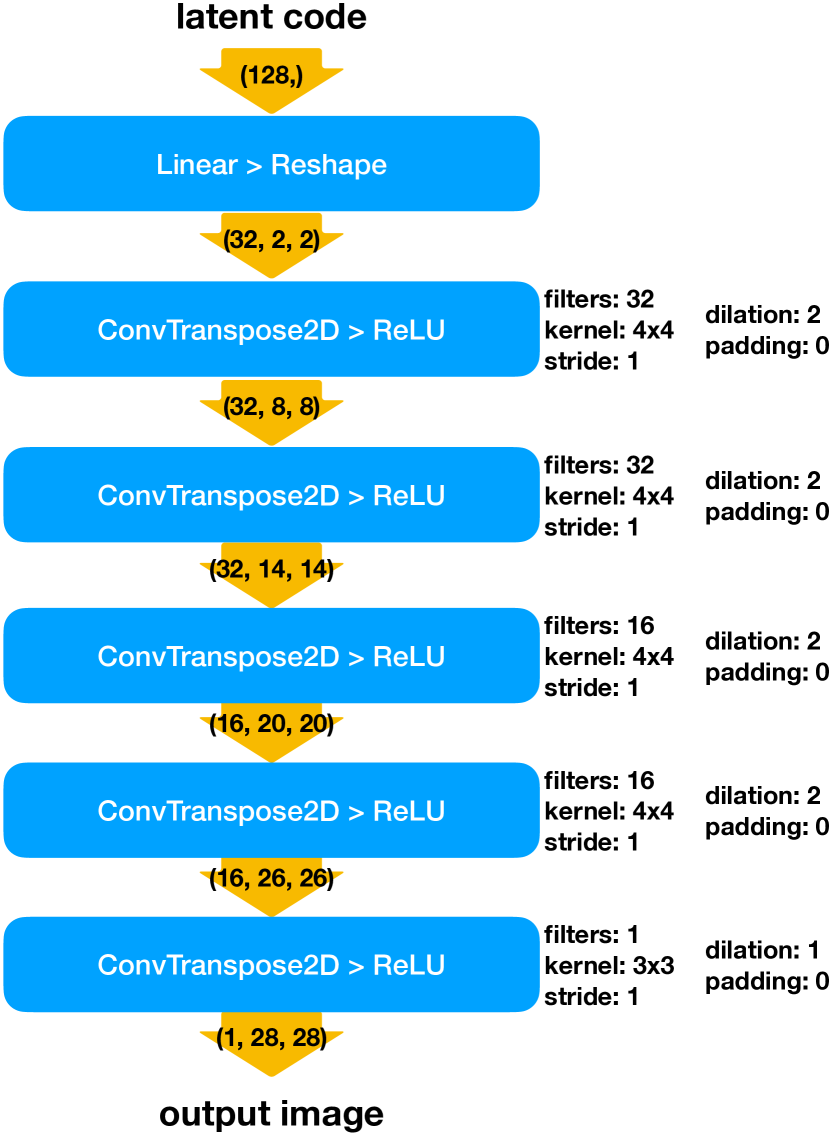
For this simulation, two deep convolutional VAEs were trained on images of 1s1𝑠1s and 888s, respectively; the trained decoders Di:128[0,1]28×28:subscript𝐷𝑖superscript128superscript012828D_{i}:\mathbb{R}^{128}\to[0,1]^{28\times 28}, i=1,8𝑖18i=1,8 from each VAE were used as the Lipschitz-continuous deep generative networks for the demixing problem. A description of the network architecture and training method for the VAEs is detailed in Further Numerics Details. We claim no novelty for our VAE or decoder architecture; extensions of VAEs involving convolutional layers appear in existing work [16, 24]. The digits used to train each VAE were a subclass of the MNIST database [3] containing only images of the digits 111 and 888. Each group of digits was randomly parititioned into training, validation and test sets. Only training and validation sets were used in the training of the VAEs.

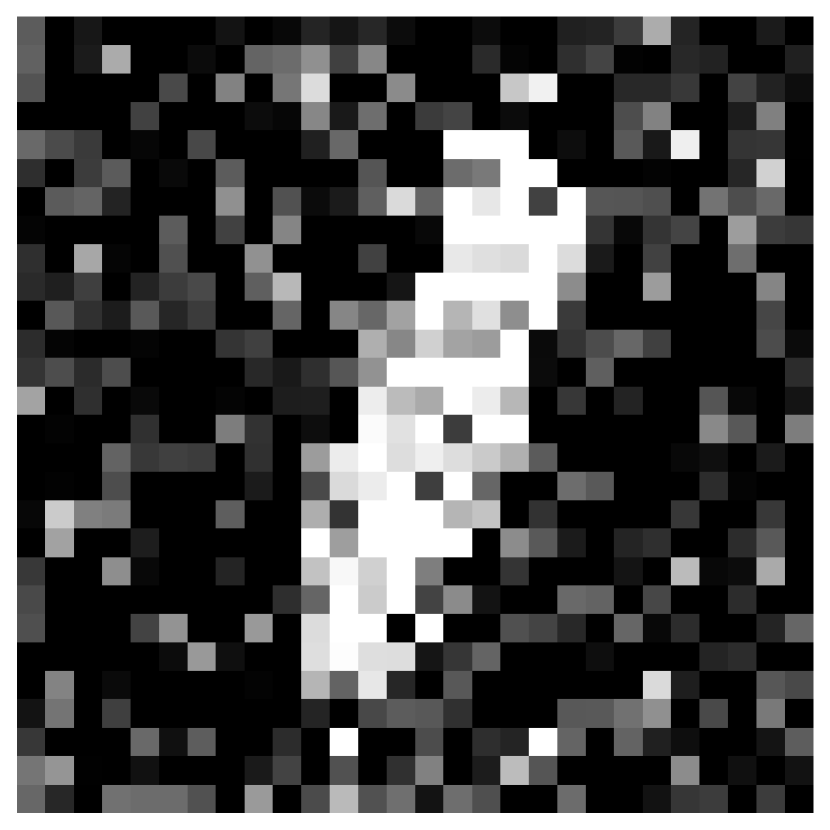
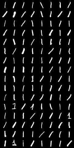
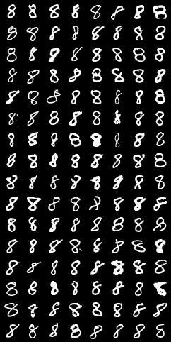
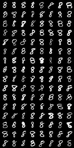
Two ground-truth images (cf. 1(a) & 1(b), resp.) were randomly sampled from the test partition of each dataset and mixed according to (1), where the mixing matrix had iid normal random entries (cf. 1(c)). In particular, where x8[0,1]28×28subscript𝑥8superscript012828x_{8}\in[0,1]^{28\times 28} is the (vectorized) grayscale image of an 888 and x1[0,1]28×28subscript𝑥1superscript012828x_{1}\in[0,1]^{28\times 28} that of a 111, the mixture is given by

b𝑏\displaystyle b =Φx8+x1,absentΦsubscript𝑥8subscript𝑥1\displaystyle=\Phi x_{8}+x_{1}, ΦΦ\displaystyle\Phi 784×784,Φijiid𝒩(0,1784).absentsuperscript784784subscriptΦ𝑖𝑗iidsimilar-to𝒩01784\displaystyle\in\mathbb{R}^{784\times 784},\Phi_{ij}\overset{\text{iid}}{\sim}\mathcal{N}(0,\tfrac{1}{784}). (3)

We did not investigate the effect of additive noise in this simulation, and leave that to a future work.

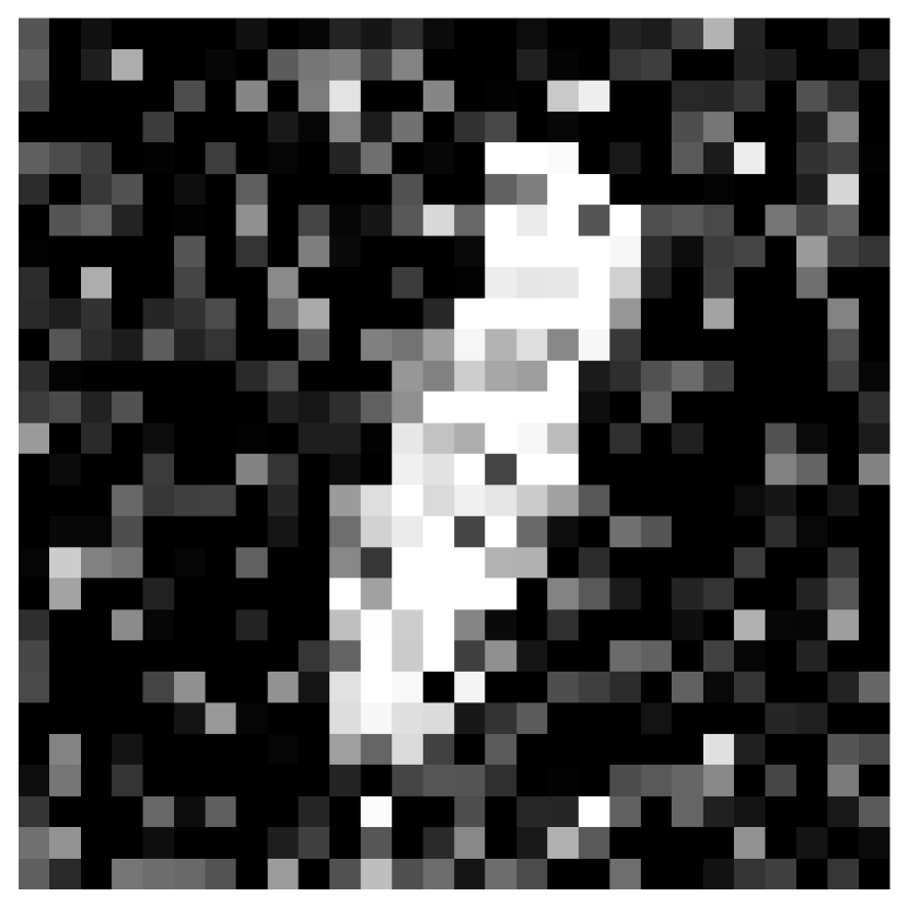
To solve the demixing problem, we used a variant of minibatch stochastic gradient descent [13] to minimize the mean-squared error (MSE) loss between the predicted mixture and the true mixture (using PyTorch [22]). Details for this numerical implementation, including pseudo-code, are provided in Further Numerics Details. The recovered mixture is depicted in 2(c), and the recovered signals, lying in the output of each generator Disubscript𝐷𝑖D_{i}, are shown in 2(a) and 2(b) for i=1,8𝑖18i=1,8, respectively.

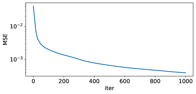
Convergence of the numerical implementation of the demixing algorithm is shown in 2(d), where we plot the MSE loss between the true mixture and the predicted mixture as a function of the iteration number. The recovered image approximating x1subscript𝑥1x_{1} had an MSE of 1.591031.59superscript1031.59\cdot 10^{-3}; that for x8subscript𝑥8x_{8}, 7.481047.48superscript1047.48\cdot 10^{-4}; and that for the mixture, 3.921043.92superscript1043.92\cdot 10^{-4}.

Refer to caption
(a) x1subscript𝑥1x_{1}
Refer to caption
(b) x8subscript𝑥8x_{8}
Refer to caption
(c) b𝑏b
image MSE
111 1.591031.59superscript1031.59\cdot 10^{-3}
888 7.481047.48superscript1047.48\cdot 10^{-4}
mixture 3.921043.92superscript1043.92\cdot 10^{-4}
(a) Final MSE
Refer to caption
(a) x^1subscript^𝑥1\hat{x}_{1}
Refer to caption
(b) x^8subscript^𝑥8\hat{x}_{8}
Refer to caption
(c) b^^𝑏\hat{b}
Refer to caption
(d) Mixture MSE vs. iteration number
Figure 2: Demixing results for two deep generative networks. (a) & (b) Ground-truth images used to create (c) the mixture. (e) & (f) The recovered images are shown beside (g) the recovered mixture. (d) Final MSE for (e–g), resp. (h) A plot of mixture MSE vs. iteration number (log-y-scale)

6 Conclusion

We prove a sample complexity bound for approximately solving the Lipschitz demixing problem with high probability on the subgaussian matrix A𝐴A. This result extends existing work from CS with Lipschitz signals and Gaussian random matrices to the demixing problem with Lipschitz signals and K𝐾K-subgaussian matrices. We establish an improved dependence on the subgaussian constant K𝐾K appearing in the deviation inequality for subgaussian mixing matrices. We connect the demixing problem for Lipschitz signals to demixing for GNNs, noting that many popular GNNs are Lipschitz. To support the theory, we provide numerical simulations for demixing images of handwritten digits. Through these simulations we suggest a viable algorithm for demixing with trained GNNs, and demonstrate efficacy of the algorithm’s performance on a particular example.

Further analysis into the demixing of Lipschitz signals would be an interesting subject of future study — for instance, in the case where the mixing is not random, or where the networks remain untrained. For example, it would be of both theoretical and practical interest to analyze signal recovery in the setting where two signals each in the range of a GNN are mixed without the subgaussian mixing matrix: b=x+y+η𝑏superscript𝑥superscript𝑦𝜂b=x^{*}+y^{*}+\eta. Here, establishing error bounds for approximate signal recovery may depend on the underlying geometric structure of the GNNs.

Additionally, theoretical analysis and thorough empirical exploration of our numerical algorithm remain open questions. For example, whether a convergence guarantee exists for the algorithm we have proposed, using GNNs, remains unknown. Further, we have chosen a particular initialization of the algorithm, but have not analyzed its effect on signal recovery in detail. A comparison of VAEs’ performance on the demixing problem using other datasets would be of interest, as would a comparison between VAEs and other GNNs such as GANs. Additionally, it could be worthwhile to validate numerically the effect of noise on demixing performance.

Finally, a further investigation may also wish to examine the case where the GNNs used as the Lipschitz functions G𝐺G and H𝐻H themselves have random weights. Such untrained networks have recently garnered attention as good structural priors for natural images [9, 10, 17], making them of potential interest to demixing.

Acknowledgments

I would like to thank Drs. Babhru Joshi, Yaniv Plan, and Özgür Yilmaz for helpful discussion in the development and communication of this work.

References

  • [1] Ashish Bora, Ajil Jalal, Eric Price, and Alexandros G Dimakis. Compressed sensing using generative models. In International Conference on Machine Learning, pages 537–546, 2017.
  • [2] Jinchi Chen and Yulong Liu. Stable recovery of structured signals from corrupted sub-gaussian measurements. IEEE Transactions on Information Theory, 65(5):2976–2994, 2018.
  • [3] Li Deng. The MNIST database of handwritten digit images for machine learning research. IEEE Signal Processing Magazine, 29(6):141–142, 2012.
  • [4] Sjoerd Dirksen. Tail bounds via generic chaining. Electronic Journal of Probability, 20, 2015.
  • [5] Carl Doersch. Tutorial on variational autoencoders. arXiv preprint arXiv:1606.05908, 2016.
  • [6] Ian Goodfellow. Tutorial: Generative adversarial networks. In Proceedings of Neural Information Processing Systems, 2016.
  • [7] Ian Goodfellow, Jean Pouget-Abadie, Mehdi Mirza, Bing Xu, David Warde-Farley, Sherjil Ozair, Aaron Courville, and Yoshua Bengio. Generative adversarial nets. In Advances in Neural Information Processing Systems, pages 2672–2680, 2014.
  • [8] Moritz Hardt, Ben Recht, and Yoram Singer. Train faster, generalize better: Stability of stochastic gradient descent. In International Conference on Machine Learning, pages 1225–1234, 2016.
  • [9] R Heckel et al. Deep decoder: Concise image representations from untrained non-convolutional networks. In International Conference on Learning Representations, 2019.
  • [10] Reinhard Heckel and Mahdi Soltanolkotabi. Compressive sensing with un-trained neural networks: Gradient descent finds the smoothest approximation. In International Conference on Machine Learning, 2020.
  • [11] Ajil Jalal, Liu Liu, Alexandros G Dimakis, and Constantine Caramanis. Robust compressed sensing of generative models. arXiv preprint arXiv:2006.09461, 2020.
  • [12] Halyun Jeong, Xiaowei Li, Yaniv Plan, and Özgür Yilmaz. Non-gaussian random matrices on sets: Optimal tail dependence and applications. In 2019 13th International conference on Sampling Theory and Applications (SampTA), pages 1–5. IEEE, 2019.
  • [13] Diederik P Kingma and Jimmy Ba. Adam: A method for stochastic optimization. arXiv preprint arXiv:1412.6980, 2014.
  • [14] Diederik P Kingma and Max Welling. Auto-encoding variational Bayes. arXiv preprint arXiv:1312.6114, 2013.
  • [15] Diederik P Kingma and Max Welling. An introduction to variational autoencoders. Foundations and Trends in Machine Learning, pages 1–18, 2019. arXiv preprint arXiv:1906.02691.
  • [16] Tejas D Kulkarni, William F Whitney, Pushmeet Kohli, and Josh Tenenbaum. Deep convolutional inverse graphics network. In Advances in Neural Information Processing Systems, pages 2539–2547, 2015.
  • [17] Victor Lempitsky, Andrea Vedaldi, and Dmitry Ulyanov. Deep image prior. In 2018 IEEE/CVF Conference on Computer Vision and Pattern Recognition, pages 9446–9454. IEEE, 2018.
  • [18] Christopher Liaw, Abbas Mehrabian, Yaniv Plan, and Roman Vershynin. A simple tool for bounding the deviation of random matrices on geometric sets. In Geometric aspects of functional analysis, pages 277–299. Springer, 2017.
  • [19] David JC MacKay. Information theory, inference and learning algorithms. Cambridge University Press, 2003.
  • [20] Michael B McCoy and Joel A Tropp. Sharp recovery bounds for convex demixing, with applications. Foundations of Computational Mathematics, 14(3):503–567, 2014.
  • [21] Stephen Odaibo. Tutorial: Deriving the standard variational autoencoder (vae) loss function. arXiv preprint arXiv:1907.08956, 2019.
  • [22] Adam Paszke, Sam Gross, Soumith Chintala, Gregory Chanan, Edward Yang, Zachary DeVito, Zeming Lin, Alban Desmaison, Luca Antiga, and Adam Lerer. Automatic differentiation in PyTorch. In NIPS Autodiff Workshop, 2017.
  • [23] Yaniv Plan and Roman Vershynin. The generalized Lasso with non-linear observations. IEEE Transactions on Information Theory, 62(3):1528–1537, 2016.
  • [24] Yunchen Pu, Zhe Gan, Ricardo Henao, Xin Yuan, Chunyuan Li, Andrew Stevens, and Lawrence Carin. Variational autoencoder for deep learning of images, labels and captions. In Advances in Neural Information Processing Systems, pages 2352–2360, 2016.
  • [25] Alec Radford, Luke Metz, and Soumith Chintala. Unsupervised representation learning with deep convolutional generative adversarial networks. arXiv preprint arXiv:1511.06434, 2015.
  • [26] Mohammadreza Soltani. Provable algorithms for nonlinear models in machine learning and signal processing. PhD thesis, Iowa State University, 2019.
  • [27] Mohammadreza Soltani and Chinmay Hegde. Demixing sparse signals from nonlinear observations. In 2016 50th Asilomar Conference on Signals, Systems and Computers, 11 2016.
  • [28] Michel Talagrand. The generic chaining: Upper and lower bounds for stochastic processes. Springer, New York;Berlin;, 2005.
  • [29] Roman Vershynin. High-dimensional probability: An introduction with applications in data science, volume 47. Cambridge University Press, 2018.
  • [30] Xiaohan Wei, Zhuoran Yang, and Zhaoran Wang. On the statistical rate of nonlinear recovery in generative models with heavy-tailed data. In International Conference on Machine Learning, pages 6697–6706, 2019.

Appendix A Proofs for §§\S3

A.1 Auxiliary results

Proposition \theprop (Gaussian complexity for |𝒯|=T𝒯𝑇|\mathcal{T}|=T).

Assume that |𝒯|=T<𝒯𝑇|\mathcal{T}|=T<\infty. Observe

w(𝒯)𝑤𝒯\displaystyle w(\mathcal{T}) ClogTdiam(𝒯);absent𝐶𝑇diam𝒯\displaystyle\leq C\sqrt{\log T}\operatorname{diam}(\mathcal{T}); 13[w(𝒯)+rad(𝒯)]13delimited-[]𝑤𝒯rad𝒯\displaystyle\frac{1}{3}\left[w(\mathcal{T})+\operatorname{rad}(\mathcal{T})\right] γ(𝒯)2[w(T)+infy𝒯y2].absent𝛾𝒯2delimited-[]𝑤𝑇subscriptinfimum𝑦𝒯subscriptnorm𝑦2\displaystyle\leq\gamma(\mathcal{T})\leq 2\left[w(T)+\inf_{y\in\mathcal{T}}\|y\|_{2}\right].
Proof of subsection A.1.

The bound on w(𝒯)𝑤𝒯w(\mathcal{T}) follows from [29, Exercise 7.5.10], and the bounds on γ(𝒯)𝛾𝒯\gamma(\mathcal{T}) follow from [29, Exercise 7.6.9]. ∎

A.2 Proof of Section 3

Proof of Section 3.

Recall the definition of Xzsubscript𝑋𝑧X_{z} in (4). Observe that for any fixed zn×m𝑧superscript𝑛superscript𝑚z\in\mathbb{R}^{n}\times\mathbb{R}^{m}, Xzsubscript𝑋𝑧X_{z} is a subgaussian random variable. For example, if z𝕊n+m1𝑧superscript𝕊𝑛𝑚1z\in\mathbb{S}^{n+m-1}, it holds that

{|Xz|CK~t}exp(t2).subscript𝑋𝑧𝐶~𝐾𝑡superscript𝑡2\displaystyle\mathbb{P}\left\{|X_{z}|\geq C\tilde{K}t\right\}\leq\exp(-t^{2}).

Consequently, for any zn×m𝑧superscript𝑛superscript𝑚z\in\mathbb{R}^{n}\times\mathbb{R}^{m},

{|Xz|mz2CK~t}exp(mt2).subscript𝑋𝑧𝑚subscriptnorm𝑧2𝐶~𝐾𝑡𝑚superscript𝑡2\displaystyle\mathbb{P}\left\{\frac{|X_{z}|}{\sqrt{m}\|z\|_{2}}\geq C\tilde{K}t\right\}\leq\exp(-mt^{2}).

Substituting ε:=CtK~assign𝜀𝐶𝑡~𝐾\varepsilon:=Ct\tilde{K}, bounding the probability by a quantity f𝑓f gives

{Bz2m(1+ε)z2}conditional-setsubscriptnorm𝐵𝑧2𝑚1𝜀evaluated-at𝑧2\displaystyle\mathbb{P}\left\{\frac{\|Bz\|_{2}}{\sqrt{m}}\geq(1+\varepsilon)\|z\|_{2}\right\} exp(cmε2K~2)=f,absent𝑐𝑚superscript𝜀2superscript~𝐾2𝑓\displaystyle\leq\exp\left(-\frac{cm\varepsilon^{2}}{\tilde{K}^{2}}\right)=f, ε𝜀\displaystyle\varepsilon =CK~2mlog(1f).absent𝐶superscript~𝐾2𝑚1𝑓\displaystyle=\sqrt{\frac{C\tilde{K}^{2}}{m}\log\left(\frac{1}{f}\right)}. (4)

Next, our goal is to construct a chain of δisubscript𝛿𝑖\delta_{i}-nets on F(𝔹)𝐹𝔹F(\mathbb{B}). We do this by constructing a chain of nets on 𝔹𝔹\mathbb{B}, M:={Mi}i=0assign𝑀superscriptsubscriptsubscript𝑀𝑖𝑖0M:=\{M_{i}\}_{i=0}^{\ell}, for which each net Misubscript𝑀𝑖M_{i} will be a product of a net Mi(1)superscriptsubscript𝑀𝑖1M_{i}^{(1)} on Bk(r)superscript𝐵𝑘𝑟B^{k}(r) and Mi(2)superscriptsubscript𝑀𝑖2M_{i}^{(2)} on Bk(r)superscript𝐵superscript𝑘superscript𝑟B^{k^{\prime}}(r^{\prime}). In particular, for Bk(r),Bk(r)superscript𝐵𝑘𝑟superscript𝐵superscript𝑘superscript𝑟B^{k}(r),B^{k^{\prime}}(r^{\prime}) [29, Corollary 4.2.13] gives the existence of ηisubscript𝜂𝑖\eta_{i}-nets Mi(1)superscriptsubscript𝑀𝑖1M_{i}^{(1)} and ηisuperscriptsubscript𝜂𝑖\eta_{i}^{\prime}-nets Mi(2)superscriptsubscript𝑀𝑖2M_{i}^{(2)} respectively satisfying

log|Mi(1)|superscriptsubscript𝑀𝑖1\displaystyle\log|M_{i}^{(1)}| klog(1+2rηi),absent𝑘12𝑟subscript𝜂𝑖\displaystyle\leq k\log(1+\frac{2r}{\eta_{i}}), log|Mi(2)|superscriptsubscript𝑀𝑖2\displaystyle\log|M_{i}^{(2)}| klog(1+2rηi).absentsuperscript𝑘12superscript𝑟superscriptsubscript𝜂𝑖\displaystyle\leq k^{\prime}\log(1+\frac{2r^{\prime}}{\eta_{i}^{\prime}}).

Choose:

ηi:=δi2LG,ηi:=δi2LH,whereδi:=δ0/2i,i[],formulae-sequenceassignsubscript𝜂𝑖subscript𝛿𝑖2subscript𝐿𝐺formulae-sequenceassignsuperscriptsubscript𝜂𝑖subscript𝛿𝑖2subscript𝐿𝐻whereformulae-sequenceassignsubscript𝛿𝑖subscript𝛿0superscript2𝑖𝑖delimited-[]\displaystyle\eta_{i}:=\frac{\delta_{i}}{\sqrt{2}L_{G}},\eta_{i}^{\prime}:=\frac{\delta_{i}}{\sqrt{2}L_{H}},\quad\text{where}\quad\delta_{i}:=\delta_{0}/2^{i},i\in[\ell],

and where δ0>0subscript𝛿00\delta_{0}>0 is any number satisfying δ0<cδK~1subscript𝛿0𝑐𝛿superscript~𝐾1\delta_{0}<c\delta\tilde{K}^{-1} for some absolute constant c>0𝑐0c>0. Then,

log|Mi|subscript𝑀𝑖\displaystyle\log|M_{i}| =log|Mi(1)|+log|Mi(2)|klog(2icrLGδ0)+klog(2icrLHδ0)absentsuperscriptsubscript𝑀𝑖1superscriptsubscript𝑀𝑖2𝑘superscript2𝑖𝑐𝑟subscript𝐿𝐺subscript𝛿0superscript𝑘superscript2𝑖𝑐superscript𝑟subscript𝐿𝐻subscript𝛿0\displaystyle=\log|M_{i}^{(1)}|+\log|M_{i}^{(2)}|\leq k\log\left(\frac{2^{i}crL_{G}}{\delta_{0}}\right)+k^{\prime}\log\left(\frac{2^{i}cr^{\prime}L_{H}}{\delta_{0}}\right)
=i(k+k)log2+klog(crLGδ0)+klog(crLHδ0)absent𝑖𝑘superscript𝑘2𝑘𝑐𝑟subscript𝐿𝐺subscript𝛿0superscript𝑘𝑐superscript𝑟subscript𝐿𝐻subscript𝛿0\displaystyle=i(k+k^{\prime})\log 2+k\log\left(\frac{crL_{G}}{\delta_{0}}\right)+k^{\prime}\log\left(\frac{cr^{\prime}L_{H}}{\delta_{0}}\right)

Observe that Ni:=F(Mi)assignsubscript𝑁𝑖𝐹subscript𝑀𝑖N_{i}:=F(M_{i}) is a δisubscript𝛿𝑖\delta_{i}-net for F(𝔹)𝐹𝔹F(\mathbb{B}): for any (u,v)𝔹𝑢𝑣𝔹(u,v)\in\mathbb{B} there exists (u,v)Misuperscript𝑢superscript𝑣subscript𝑀𝑖(u^{\prime},v^{\prime})\in M_{i} with

F(u,v)F(u,v)2subscriptnorm𝐹𝑢𝑣𝐹superscript𝑢superscript𝑣2\displaystyle\|F(u,v)-F(u^{\prime},v^{\prime})\|_{2} =G(u)G(u)22+H(v)H(v)22absentsuperscriptsubscriptnorm𝐺𝑢𝐺superscript𝑢22superscriptsubscriptnorm𝐻𝑣𝐻superscript𝑣22\displaystyle=\sqrt{\|G(u)-G(u^{\prime})\|_{2}^{2}+\|H(v)-H(v^{\prime})\|_{2}^{2}}
LG2uu22+LHvv22δiabsentsuperscriptsubscript𝐿𝐺2superscriptsubscriptnorm𝑢superscript𝑢22subscript𝐿𝐻superscriptsubscriptnorm𝑣superscript𝑣22subscript𝛿𝑖\displaystyle\leq\sqrt{L_{G}^{2}\|u-u^{\prime}\|_{2}^{2}+L_{H}\|v-v^{\prime}\|_{2}^{2}}\leq\delta_{i}

Next, define

Ti:={zi+1zi:zi+1Ni+1,ziNi}assignsubscript𝑇𝑖conditional-setsubscript𝑧𝑖1subscript𝑧𝑖formulae-sequencesubscript𝑧𝑖1subscript𝑁𝑖1subscript𝑧𝑖subscript𝑁𝑖\displaystyle T_{i}:=\{z_{i+1}-z_{i}:z_{i+1}\in N_{i+1},z_{i}\in N_{i}\}

and observe that Tisubscript𝑇𝑖T_{i} has cardinality satisfying

log|Ti|subscript𝑇𝑖\displaystyle\log|T_{i}| log(|Ni+1||Ni|)log(|Mi+1||Mi|)absentsubscript𝑁𝑖1subscript𝑁𝑖subscript𝑀𝑖1subscript𝑀𝑖\displaystyle\leq\log(|N_{i+1}||N_{i}|)\leq\log(|M_{i+1}||M_{i}|)
C(2i+1)(k+k)+2klog(crLGδ0)+2klog(crLHδ0).absent𝐶2𝑖1𝑘superscript𝑘2𝑘𝑐𝑟subscript𝐿𝐺subscript𝛿02superscript𝑘𝑐superscript𝑟subscript𝐿𝐻subscript𝛿0\displaystyle\leq C(2i+1)(k+k^{\prime})+2k\log\left(\frac{crL_{G}}{\delta_{0}}\right)+2k^{\prime}\log\left(\frac{cr^{\prime}L_{H}}{\delta_{0}}\right).

Eventually, for a collection (εi,fi)subscript𝜀𝑖subscript𝑓𝑖(\varepsilon_{i},f_{i}) connected as in (4), we will union bound to obtain

{Bζm(1+εi)ζ,i,ζTi}1i=01|Ti|fi.formulae-sequencenorm𝐵𝜁𝑚1subscript𝜀𝑖norm𝜁for-all𝑖for-all𝜁subscript𝑇𝑖1superscriptsubscript𝑖01subscript𝑇𝑖subscript𝑓𝑖\displaystyle\mathbb{P}\left\{\frac{\|B\zeta\|}{\sqrt{m}}\leq(1+\varepsilon_{i})\|\zeta\|,\forall i,\forall\zeta\in T_{i}\right\}\geq 1-\sum_{i=0}^{\ell-1}|T_{i}|f_{i}. (5)

We start by ensuring the right-hand side of the above expression is small. Using

log(|Ti|fi)subscript𝑇𝑖subscript𝑓𝑖\displaystyle\log(|T_{i}|f_{i}) =log|Ti|+log(fi)absentsubscript𝑇𝑖subscript𝑓𝑖\displaystyle=\log|T_{i}|+\log(f_{i})
C(2i+1)(k+k)+2klog(crLGδ0)+2klog(crLHδ0)+log(fi),absent𝐶2𝑖1𝑘superscript𝑘2𝑘𝑐𝑟subscript𝐿𝐺subscript𝛿02superscript𝑘𝑐superscript𝑟subscript𝐿𝐻subscript𝛿0subscript𝑓𝑖\displaystyle\leq C(2i+1)(k+k^{\prime})+2k\log\left(\frac{crL_{G}}{\delta_{0}}\right)+2k^{\prime}\log\left(\frac{cr^{\prime}L_{H}}{\delta_{0}}\right)+\log(f_{i}), (6)

and choosing

m2klog(crLGδ0)+2klog(crLHδ0),log(fi)=(4m3+C(3i+1)(k+k)),formulae-sequence𝑚2𝑘𝑐𝑟subscript𝐿𝐺subscript𝛿02superscript𝑘𝑐superscript𝑟subscript𝐿𝐻subscript𝛿0subscript𝑓𝑖4𝑚3𝐶3𝑖1𝑘superscript𝑘\displaystyle m\geq 2k\log\left(\frac{crL_{G}}{\delta_{0}}\right)+2k^{\prime}\log\left(\frac{cr^{\prime}L_{H}}{\delta_{0}}\right),\qquad\log(f_{i})=-\left(\frac{4m}{3}+C(3i+1)(k+k^{\prime})\right),

gives

log(|Ti|fi)Ci(k+k)m3.subscript𝑇𝑖subscript𝑓𝑖𝐶𝑖𝑘superscript𝑘𝑚3\displaystyle\log(|T_{i}|f_{i})\leq-Ci(k+k^{\prime})-\frac{m}{3}.

In particular,

i=01|Ti|fiexp(m3)i=01exp(Ci(k+k))exp(m3)11eCCexp(m3).superscriptsubscript𝑖01subscript𝑇𝑖subscript𝑓𝑖𝑚3superscriptsubscript𝑖01𝐶𝑖𝑘superscript𝑘𝑚311superscript𝑒𝐶𝐶𝑚3\displaystyle\sum_{i=0}^{\ell-1}|T_{i}|f_{i}\leq\exp\left(-\frac{m}{3}\right)\sum_{i=0}^{\ell-1}\exp\left(-Ci(k+k^{\prime})\right)\leq\exp\left(-\frac{m}{3}\right)\frac{1}{1-e^{-C}}\leq C\exp\left(-\frac{m}{3}\right).

With the present choices, the expression for εisubscript𝜀𝑖\varepsilon_{i} becomes, using (4),

εisubscript𝜀𝑖\displaystyle\varepsilon_{i} =CK~2mlog(1fi)=CK~1+(3i+1)(k+k)m.absent𝐶superscript~𝐾2𝑚1subscript𝑓𝑖𝐶~𝐾13𝑖1𝑘superscript𝑘𝑚\displaystyle=\sqrt{\frac{C\tilde{K}^{2}}{m}\log\left(\frac{1}{f_{i}}\right)}=C\tilde{K}\sqrt{1+\frac{(3i+1)(k+k^{\prime})}{m}}.

Now for any zF(𝔹)𝑧𝐹𝔹z\in F(\mathbb{B}), we can write

z=z0+(z1z0)++(zz1)+zf𝑧subscript𝑧0subscript𝑧1subscript𝑧0subscript𝑧subscript𝑧1superscript𝑧𝑓\displaystyle z=z_{0}+(z_{1}-z_{0})+\cdots+(z_{\ell}-z_{\ell-1})+z^{f}

where ziNi,zf:=zzformulae-sequencesubscript𝑧𝑖subscript𝑁𝑖assignsuperscript𝑧𝑓𝑧subscript𝑧z_{i}\in N_{i},z^{f}:=z-z_{\ell}. Using (5), since ζi=zi+1ziTisubscript𝜁𝑖subscript𝑧𝑖1subscript𝑧𝑖subscript𝑇𝑖\zeta_{i}=z_{i+1}-z_{i}\in T_{i}, it holds with probability at least 1Cexp(m/3)1𝐶𝑚31-C\exp(-m/3) that

m1/2i=01Bζi2superscript𝑚12superscriptsubscript𝑖01subscriptnorm𝐵subscript𝜁𝑖2\displaystyle m^{-1/2}\sum_{i=0}^{\ell-1}\|B\zeta_{i}\|_{2} i=01(1+εi)ζi2δ0i=012i(1+εi)absentsuperscriptsubscript𝑖011subscript𝜀𝑖subscriptnormsubscript𝜁𝑖2subscript𝛿0superscriptsubscript𝑖01superscript2𝑖1subscript𝜀𝑖\displaystyle\leq\sum_{i=0}^{\ell-1}(1+\varepsilon_{i})\|\zeta_{i}\|_{2}\leq\delta_{0}\sum_{i=0}^{\ell-1}2^{-i}(1+\varepsilon_{i})
δ0i=012i(1+CK~1+(3i+1)(k+k)m)absentsubscript𝛿0superscriptsubscript𝑖01superscript2𝑖1𝐶~𝐾13𝑖1𝑘superscript𝑘𝑚\displaystyle\leq\delta_{0}\sum_{i=0}^{\ell-1}2^{-i}\left(1+C\tilde{K}\sqrt{1+\frac{(3i+1)(k+k^{\prime})}{m}}\right)
Cδ0K~i=011+3i+12iCδ0K~<δ2.absent𝐶subscript𝛿0~𝐾superscriptsubscript𝑖0113𝑖1superscript2𝑖𝐶subscript𝛿0~𝐾𝛿2\displaystyle\leq C\delta_{0}\tilde{K}\sum_{i=0}^{\ell-1}\frac{1+\sqrt{3i+1}}{2^{i}}\leq C\delta_{0}\tilde{K}<\frac{\delta}{2}.

Also observe that zf2δ0/2subscriptnormsuperscript𝑧𝑓2subscript𝛿0superscript2\|z^{f}\|_{2}\leq\delta_{0}/2^{\ell} by construction.

Now, using Theorem 2 with 𝒯:=𝕊n+m1assign𝒯superscript𝕊𝑛𝑚1\mathcal{T}:=\mathbb{S}^{n+m-1} we have

supz𝒯|Bz2m1|CK~[n+mm+1]subscriptsupremum𝑧𝒯subscriptnorm𝐵𝑧2𝑚1𝐶~𝐾delimited-[]𝑛𝑚𝑚1\displaystyle\sup_{z\in\mathcal{T}}\left|\frac{\|Bz\|_{2}}{\sqrt{m}}-1\right|\leq C\tilde{K}\left[\sqrt{\frac{n+m}{m}}+1\right]

with probability at least 1exp(m)1𝑚1-\exp(-m). In particular, with the stated probability,

BmCK~(2+n+mm).norm𝐵𝑚𝐶~𝐾2𝑛𝑚𝑚\displaystyle\left\|\frac{B}{\sqrt{m}}\right\|\leq C\tilde{K}\left(2+\sqrt{\frac{n+m}{m}}\right).

Therefore, with probability at least 1exp(m)1𝑚1-\exp(-m) we have

m1/2Bzf2Cδ0K~2(2+n+mm)Cδ0K~<δ2,superscript𝑚12subscriptnorm𝐵superscript𝑧𝑓2𝐶subscript𝛿0~𝐾superscript22𝑛𝑚𝑚𝐶subscript𝛿0~𝐾𝛿2\displaystyle m^{-1/2}\|Bz^{f}\|_{2}\leq C\delta_{0}\tilde{K}2^{-\ell}\left(2+\sqrt{\frac{n+m}{m}}\right)\leq C\delta_{0}\tilde{K}<\frac{\delta}{2},

achieved by taking Clog(2+κ1)𝐶2superscript𝜅1\ell\geq C\log(2+\kappa^{-1}) where κ:=m/nassign𝜅𝑚𝑛\kappa:=m/n is the aspect ratio of A𝐴A.

Combining the above results, and noting that it is possible to choose z=z0superscript𝑧subscript𝑧0z^{\prime}=z_{0}, it holds with probability at least 1exp(cm)1𝑐𝑚1-\exp(-cm) that

m1/2B(zz)2=m1/2B(zz0)2m1/2Bzf2+m1/2i=01Bζi2<δ.superscript𝑚12subscriptnorm𝐵𝑧superscript𝑧2superscript𝑚12subscriptnorm𝐵𝑧subscript𝑧02superscript𝑚12subscriptnorm𝐵superscript𝑧𝑓2superscript𝑚12superscriptsubscript𝑖01subscriptnorm𝐵subscript𝜁𝑖2𝛿\displaystyle m^{-1/2}\|B(z-z^{\prime})\|_{2}=m^{-1/2}\|B(z-z_{0})\|_{2}\leq m^{-1/2}\|Bz^{f}\|_{2}+m^{-1/2}\sum_{i=0}^{\ell-1}\|B\zeta_{i}\|_{2}<\delta.

A.3 Proof of Section 3

Proof of Section 3.

Observe that there exists a net M:=M(1)×M(2)assign𝑀superscript𝑀1superscript𝑀2M:=M^{(1)}\times M^{(2)} for 𝔹𝔹\mathbb{B} where M(1)superscript𝑀1M^{(1)} is a δ2LG𝛿2subscript𝐿𝐺\frac{\delta}{\sqrt{2}L_{G}}-net for Bk(r)superscript𝐵𝑘𝑟B^{k}(r) and M(2)superscript𝑀2M^{(2)} is a δ2LH𝛿2subscript𝐿𝐻\frac{\delta}{\sqrt{2}L_{H}}-net for Bk(r)superscript𝐵superscript𝑘superscript𝑟B^{k^{\prime}}(r^{\prime}), with

log|M|log|M(1)|+log|M(2)|klog(1+22LGrδ)+klog(1+22LHrδ).𝑀superscript𝑀1superscript𝑀2𝑘122subscript𝐿𝐺𝑟𝛿superscript𝑘122subscript𝐿𝐻superscript𝑟𝛿\displaystyle\log|M|\leq\log|M^{(1)}|+\log|M^{(2)}|\leq k\log\left(1+\frac{2\sqrt{2}L_{G}r}{\delta}\right)+k^{\prime}\log\left(1+\frac{2\sqrt{2}L_{H}r^{\prime}}{\delta}\right).

By construction, F(M)={(G(u),H(v)):(u,v)M}𝐹𝑀conditional-set𝐺𝑢𝐻𝑣𝑢𝑣𝑀F(M)=\{(G(u),H(v)):(u,v)\in M\} is a δ𝛿\delta-net for F(𝔹)𝐹𝔹F(\mathbb{B}). In particular, for any z,zF(𝔹)𝑧superscript𝑧𝐹𝔹z,z^{\prime}\in F(\mathbb{B}) there are z1,z2F(M)subscript𝑧1subscript𝑧2𝐹𝑀z_{1},z_{2}\in F(M) such that

zz2zz12+z1z22+z2z2z1z22+2δ.subscriptnorm𝑧superscript𝑧2subscriptnorm𝑧subscript𝑧12subscriptnormsubscript𝑧1subscript𝑧22subscriptnormsubscript𝑧2superscript𝑧2subscriptnormsubscript𝑧1subscript𝑧222𝛿\displaystyle\|z-z^{\prime}\|_{2}\leq\|z-z_{1}\|_{2}+\|z_{1}-z_{2}\|_{2}+\|z_{2}-z^{\prime}\|_{2}\leq\|z_{1}-z_{2}\|_{2}+2\delta. (7)

Moreover, for these points, applying Section 3 for a possibly larger net M𝑀M gives

B(z1z2)2B(z1z)2+B(zz)2+B(zz2)2B(zz)2+Cδm.subscriptnorm𝐵subscript𝑧1subscript𝑧22subscriptnorm𝐵subscript𝑧1𝑧2subscriptnorm𝐵𝑧superscript𝑧2subscriptnorm𝐵superscript𝑧subscript𝑧22subscriptnorm𝐵𝑧superscript𝑧2𝐶𝛿𝑚\displaystyle\|B(z_{1}-z_{2})\|_{2}\leq\|B(z_{1}-z)\|_{2}+\|B(z-z^{\prime})\|_{2}+\|B(z^{\prime}-z_{2})\|_{2}\leq\|B(z-z^{\prime})\|_{2}+C\delta\sqrt{m}. (8)

Next, defining

𝒯:={z1z2z1z22:z1,z2F(M)},assign𝒯conditional-setsubscript𝑧1subscript𝑧2subscriptnormsubscript𝑧1subscript𝑧22subscript𝑧1subscript𝑧2𝐹𝑀\displaystyle\mathcal{T}:=\left\{\frac{z_{1}-z_{2}}{\|z_{1}-z_{2}\|_{2}}:z_{1},z_{2}\in F(M)\right\},

and noting γ(𝒯)Clog|M|𝛾𝒯𝐶𝑀\gamma(\mathcal{T})\leq C\sqrt{\log|M|} by subsection A.1, we may use Section 4 to obtain

supz1,z2F(M)|B(z1z2)2mz1z221|CK~log|M|m,subscriptsupremumsubscript𝑧1subscript𝑧2𝐹𝑀subscriptnorm𝐵subscript𝑧1subscript𝑧22𝑚subscriptnormsubscript𝑧1subscript𝑧221𝐶~𝐾𝑀𝑚\displaystyle\sup_{z_{1},z_{2}\in F(M)}\left|\frac{\|B(z_{1}-z_{2})\|_{2}}{\sqrt{m}\|z_{1}-z_{2}\|_{2}}-1\right|\leq C\tilde{K}\sqrt{\frac{\log|M|}{m}},

with probability at least 1exp(m)1𝑚1-\exp(-m). Accordingly, one has

(1α)z1z22m1/2B(z1z2)2(1+α)z1z221𝛼subscriptnormsubscript𝑧1subscript𝑧22superscript𝑚12subscriptnorm𝐵subscript𝑧1subscript𝑧221𝛼subscriptnormsubscript𝑧1subscript𝑧22\displaystyle(1-\alpha)\|z_{1}-z_{2}\|_{2}\leq m^{-1/2}\|B(z_{1}-z_{2})\|_{2}\leq(1+\alpha)\|z_{1}-z_{2}\|_{2} (9)

with probability at least 1exp(m)1𝑚1-\exp(-m) provided that

mCK~2α2(k+k)log(λK~δ)CK~2α2log|M|,λ:=max{LGr,LHr}.formulae-sequence𝑚𝐶superscript~𝐾2superscript𝛼2𝑘superscript𝑘𝜆~𝐾𝛿𝐶superscript~𝐾2superscript𝛼2𝑀assign𝜆subscript𝐿𝐺𝑟subscript𝐿𝐻superscript𝑟\displaystyle m\geq\frac{C\tilde{K}^{2}}{\alpha^{2}}(k+k^{\prime})\log\left(\frac{\lambda\tilde{K}}{\delta}\right)\geq\frac{C\tilde{K}^{2}}{\alpha^{2}}\log|M|,\qquad\lambda:=\max\{L_{G}r,L_{H}r^{\prime}\}. (10)

Combining (79) under condition (10) gives, for any z,zF(𝔹)𝑧superscript𝑧𝐹𝔹z,z^{\prime}\in F(\mathbb{B}),

(1α)zz21𝛼subscriptnorm𝑧superscript𝑧2\displaystyle(1-\alpha)\|z-z^{\prime}\|_{2} (1α)z1z22+2δm1/2B(z1z2)2+2δabsent1𝛼subscriptnormsubscript𝑧1subscript𝑧222𝛿subscriptnormsuperscript𝑚12𝐵subscript𝑧1subscript𝑧222𝛿\displaystyle\leq(1-\alpha)\|z_{1}-z_{2}\|_{2}+2\delta\leq\|m^{-1/2}B(z_{1}-z_{2})\|_{2}+2\delta
m1/2B(zz)2+4δ.absentsubscriptnormsuperscript𝑚12𝐵𝑧superscript𝑧24𝛿\displaystyle\leq\|m^{-1/2}B(z-z^{\prime})\|_{2}+4\delta.

with probability at least 1exp(cm)1𝑐𝑚1-\exp(-cm).

Remark 1 (Simplified sample complexity bound).

The expression appearing in (10),

mCK~2α2(k+k)log(λK~δ),𝑚𝐶superscript~𝐾2superscript𝛼2𝑘superscript𝑘𝜆~𝐾𝛿\displaystyle m\geq\frac{C\tilde{K}^{2}}{\alpha^{2}}(k+k^{\prime})\log\left(\frac{\lambda\tilde{K}}{\delta}\right),

is simpler (i.e., more aesthetic) than the analogous condition appearing in the statement of Section 3, but also a stronger assumption on m𝑚m, due to the definition of λ𝜆\lambda.

A.4 Proof of Theorem 1

Before proving Theorem 1, we modify [1, Lemma 4.3] so that the statement fits the present setting.

Lemma \thelem (modified [1, Lemma 4.3]).

Let B~:=[A~Im]assign~𝐵delimited-[]~𝐴subscript𝐼𝑚\tilde{B}:=\left[\begin{array}[]{rr}\tilde{A}&I_{m}\end{array}\right] where A~m×n~𝐴superscript𝑚𝑛\tilde{A}\in\mathbb{R}^{m\times n} is drawn from a distribution such that:

  1. 1.

    B~~𝐵\tilde{B} satisfies SREC(S,γ,δ)SREC𝑆𝛾𝛿\operatorname{S-REC}(S,\gamma,\delta) with probability 1p1𝑝1-p;

  2. 2.

    B~z2CK~z2subscriptnorm~𝐵𝑧2𝐶~𝐾subscriptnorm𝑧2\|\tilde{B}z\|_{2}\leq C\tilde{K}\|z\|_{2} for every fixed zn×m𝑧superscript𝑛superscript𝑚z\in\mathbb{R}^{n}\times\mathbb{R}^{m} with probability 1p1𝑝1-p.

For any zn×msuperscript𝑧superscript𝑛superscript𝑚z^{*}\in\mathbb{R}^{n}\times\mathbb{R}^{m} and noise ηm𝜂superscript𝑚\eta\in\mathbb{R}^{m}, let b=B~z+η𝑏~𝐵superscript𝑧𝜂b=\tilde{B}z^{*}+\eta. Let z^^𝑧\hat{z} satisfy

bB~z^2minzSbB~z2+ϵ.subscriptnorm𝑏~𝐵^𝑧2subscript𝑧𝑆subscriptnorm𝑏~𝐵𝑧2italic-ϵ\displaystyle\|b-\tilde{B}\hat{z}\|_{2}\leq\min_{z\in S}\|b-\tilde{B}z\|_{2}+\epsilon.

Then, with probability 12p12𝑝1-2p,

z^z2(CK~γ+1)minzSzz2+1γ(2η2+ϵ+δ).subscriptnorm^𝑧superscript𝑧2𝐶~𝐾𝛾1subscript𝑧𝑆subscriptnormsuperscript𝑧𝑧21𝛾2subscriptnorm𝜂2italic-ϵ𝛿\displaystyle\left\|\hat{z}-z^{*}\right\|_{2}\leq\left(\frac{C\tilde{K}}{\gamma}+1\right)\min_{z\in S}\left\|z^{*}-z\right\|_{2}+\frac{1}{\gamma}(2\|\eta\|_{2}+\epsilon+\delta).
Proof of subsection A.4.

We proceed as in the proof of [1, Lemma 4.3]. Define z¯argminzSzz2¯𝑧subscript𝑧𝑆subscriptnormsuperscript𝑧𝑧2\bar{z}\in\operatorname*{\arg\min}_{z\in S}\left\|z^{*}-z\right\|_{2}. Since B~~𝐵\tilde{B} satisfies SREC(S,γ,δ)SREC𝑆𝛾𝛿\operatorname{S-REC}(S,\gamma,\delta), with probability 1p1𝑝1-p, it holds with probability 1p1𝑝1-p, using the assumption on z^^𝑧\hat{z}, that

z¯z^2subscriptnorm¯𝑧^𝑧2\displaystyle\|\bar{z}-\hat{z}\|_{2} γ1(B~z¯b2+B~z^b2+δ)γ1(B~z¯b2+minzSB~zb2+δ+ε)absentsuperscript𝛾1subscriptnorm~𝐵¯𝑧𝑏2subscriptnorm~𝐵^𝑧𝑏2𝛿superscript𝛾1subscriptnorm~𝐵¯𝑧𝑏2subscript𝑧𝑆subscriptnorm~𝐵𝑧𝑏2𝛿𝜀\displaystyle\leq\gamma^{-1}\left(\|\tilde{B}\bar{z}-b\|_{2}+\|\tilde{B}\hat{z}-b\|_{2}+\delta\right)\leq\gamma^{-1}\left(\|\tilde{B}\bar{z}-b\|_{2}+\min_{z\in S}\|\tilde{B}z-b\|_{2}+\delta+\varepsilon\right)
γ1(2B~z¯b2+δ+ε)γ1(2B~(z¯z)2+δ+ε+2η2)absentsuperscript𝛾12subscriptnorm~𝐵¯𝑧𝑏2𝛿𝜀superscript𝛾12subscriptnorm~𝐵¯𝑧superscript𝑧2𝛿𝜀2subscriptnorm𝜂2\displaystyle\leq\gamma^{-1}\left(2\|\tilde{B}\bar{z}-b\|_{2}+\delta+\varepsilon\right)\leq\gamma^{-1}\left(2\|\tilde{B}(\bar{z}-z^{*})\|_{2}+\delta+\varepsilon+2\|\eta\|_{2}\right)

By assumption, it also holds with probability at least 1p1𝑝1-p that B~(z¯z)2CK~z¯z2subscriptnorm~𝐵¯𝑧superscript𝑧2𝐶~𝐾subscriptnorm¯𝑧superscript𝑧2\|\tilde{B}(\bar{z}-z^{*})\|_{2}\leq C\tilde{K}\|\bar{z}-z^{*}\|_{2}. Therefore, with probability at least 12p12𝑝1-2p,

zz^2subscriptnormsuperscript𝑧^𝑧2\displaystyle\|z^{*}-\hat{z}\|_{2} zz¯2+z¯z^2absentsubscriptnormsuperscript𝑧¯𝑧2subscriptnorm¯𝑧^𝑧2\displaystyle\leq\|z^{*}-\bar{z}\|_{2}+\|\bar{z}-\hat{z}\|_{2}
zz¯2+γ1(2B~(z¯z)2+δ+ε+2η2)absentsubscriptnormsuperscript𝑧¯𝑧2superscript𝛾12subscriptnorm~𝐵¯𝑧superscript𝑧2𝛿𝜀2subscriptnorm𝜂2\displaystyle\leq\|z^{*}-\bar{z}\|_{2}+\gamma^{-1}\left(2\|\tilde{B}(\bar{z}-z^{*})\|_{2}+\delta+\varepsilon+2\|\eta\|_{2}\right)
zz¯2+γ1(CK~z¯z2+δ+ε+2η2)absentsubscriptnormsuperscript𝑧¯𝑧2superscript𝛾1𝐶~𝐾subscriptnorm¯𝑧superscript𝑧2𝛿𝜀2subscriptnorm𝜂2\displaystyle\leq\|z^{*}-\bar{z}\|_{2}+\gamma^{-1}\left(C\tilde{K}\|\bar{z}-z^{*}\|_{2}+\delta+\varepsilon+2\|\eta\|_{2}\right)
=(1+CK~γ)zz¯2+δ+ε+2η2γabsent1𝐶~𝐾𝛾subscriptnormsuperscript𝑧¯𝑧2𝛿𝜀2subscriptnorm𝜂2𝛾\displaystyle=\left(1+\frac{C\tilde{K}}{\gamma}\right)\|z^{*}-\bar{z}\|_{2}+\frac{\delta+\varepsilon+2\|\eta\|_{2}}{\gamma}

Proof of Theorem 1.

Suppose α(0,1)𝛼01\alpha\in(0,1). By definition of A𝐴A and B:=[AmIm]assign𝐵delimited-[]𝐴𝑚subscript𝐼𝑚B:=\left[\begin{array}[]{rr}A&\sqrt{m}I_{m}\end{array}\right], the normalized mixing matrix B~:=m1/2Bassign~𝐵superscript𝑚12𝐵\tilde{B}:=m^{-1/2}B satisfies SREC(F(𝔹),1α,δ)SREC𝐹𝔹1𝛼𝛿\operatorname{S-REC}(F(\mathbb{B}),1-\alpha,\delta) with probability at least 1exp(cm)1𝑐𝑚1-\exp(-cm) when

mCK~2α2(klog(LGrδ)+klog(LHrδ)).𝑚𝐶superscript~𝐾2superscript𝛼2𝑘subscript𝐿𝐺𝑟𝛿superscript𝑘subscript𝐿𝐻superscript𝑟𝛿\displaystyle m\geq\frac{C\tilde{K}^{2}}{\alpha^{2}}\left(k\log\left(\frac{L_{G}r}{\delta}\right)+k^{\prime}\log\left(\frac{L_{H}r^{\prime}}{\delta}\right)\right).

Observe that if λ:=max{LGr,LHr}assign𝜆subscript𝐿𝐺𝑟subscript𝐿𝐻superscript𝑟\lambda:=\max\{L_{G}r,L_{H}r^{\prime}\} then mCK~2α2(k+k)log(λδ)𝑚𝐶superscript~𝐾2superscript𝛼2𝑘superscript𝑘𝜆𝛿m\geq\frac{C\tilde{K}^{2}}{\alpha^{2}}(k+k^{\prime})\log\left(\frac{\lambda}{\delta}\right) implies the above condition. Furthermore, subgaussianity of Xzsubscript𝑋𝑧X_{z} gives for any fixed zn×m𝑧superscript𝑛superscript𝑚z\in\mathbb{R}^{n}\times\mathbb{R}^{m},

|B~z2z2|CαK~z2subscriptnorm~𝐵𝑧2subscriptnorm𝑧2𝐶𝛼~𝐾subscriptnorm𝑧2\displaystyle\left|\|\tilde{B}z\|_{2}-\|z\|_{2}\right|\leq C\alpha\tilde{K}\|z\|_{2}

with probability at least 1exp(α2m)1superscript𝛼2𝑚1-\exp(-\alpha^{2}m). Choosing α:=12assign𝛼12\alpha:=\frac{1}{2} and applying subsection A.4 gives

z^z2CK~minzF(𝔹)zz2+C(2η2+δ+ε).subscriptnorm^𝑧superscript𝑧2𝐶~𝐾subscript𝑧𝐹𝔹subscriptnormsuperscript𝑧𝑧2𝐶2subscriptnorm𝜂2𝛿𝜀\displaystyle\|\hat{z}-z^{*}\|_{2}\leq C\tilde{K}\min_{z\in F(\mathbb{B})}\|z^{*}-z\|_{2}+C(2\|\eta\|_{2}+\delta+\varepsilon).

Appendix B Proofs for §§\S4

B.1 Proof of Section 4

It should be noted that the proof of Section 4 strongly resembles the proof of an analogous result, [2, Lemma 5]. We include full details here for the sake of clarity to the reader, and note that the proof requires only a handful of changes to leverage an improved Bernstein’s inequality, [12, New Bernstein’s inequality].

Theorem ([12, New Bernstein’s inequality]).

Let a=(a1,,am)𝑎subscript𝑎1subscript𝑎𝑚a=(a_{1},\ldots,a_{m}) be a fixed nonzero vector and let Y1,Ymsubscript𝑌1subscript𝑌𝑚Y_{1}\,\ldots,Y_{m} be independent, centered subexponential random vectors satisfying 𝔼|Yi|2𝔼subscript𝑌𝑖2\operatorname*{\mathbb{E}}|Y_{i}|\leq 2 and Yiψ1Ki2subscriptnormsubscript𝑌𝑖subscript𝜓1superscriptsubscript𝐾𝑖2\|Y_{i}\|_{\psi_{1}}\leq K_{i}^{2} with Ki2subscript𝐾𝑖2K_{i}\geq 2. Then, for every u0𝑢0u\geq 0,

{|i=1maiYi|u}2exp[cmin(u2i=1mai2Ki2logKi,uaK2logK)]superscriptsubscript𝑖1𝑚subscript𝑎𝑖subscript𝑌𝑖𝑢2𝑐superscript𝑢2superscriptsubscript𝑖1𝑚superscriptsubscript𝑎𝑖2superscriptsubscript𝐾𝑖2subscript𝐾𝑖𝑢subscriptnorm𝑎superscript𝐾2𝐾\displaystyle\mathbb{P}\left\{\left|\sum_{i=1}^{m}a_{i}Y_{i}\right|\geq u\right\}\leq 2\exp\left[-c\cdot\min\left(\frac{u^{2}}{\sum_{i=1}^{m}a_{i}^{2}K_{i}^{2}\log K_{i}},\frac{u}{\|a\|_{\infty}K^{2}\log K}\right)\right]

where K:=maxiKiassign𝐾subscript𝑖subscript𝐾𝑖K:=\max_{i}K_{i} and c𝑐c is an absolute constant.

We will also rely on a version of Hoeffding’s inequality for weighted sums of subgaussian random variables. We state this theorem as it appears in [29, Theorem 2.6.3].

Theorem ([29, Theorem 2.6.3]).

Let X1,,Xmsubscript𝑋1subscript𝑋𝑚X_{1},\ldots,X_{m} be independent, centered, subgaussian random variables, and a=(a1,,am)m𝑎subscript𝑎1subscript𝑎𝑚superscript𝑚a=\left(a_{1},\ldots,a_{m}\right)\in\mathbb{R}^{m}. Then, for every t0𝑡0t\geq 0, we have

{|i=1maiXi|t}2exp(ct2K2a22)superscriptsubscript𝑖1𝑚subscript𝑎𝑖subscript𝑋𝑖𝑡2𝑐superscript𝑡2superscript𝐾2superscriptsubscriptnorm𝑎22\displaystyle\mathbb{P}\left\{\left|\sum_{i=1}^{m}a_{i}X_{i}\right|\geq t\right\}\leq 2\exp\left(-\frac{ct^{2}}{K^{2}\|a\|_{2}^{2}}\right)

where K=maxiXiψ2𝐾subscript𝑖subscriptnormsubscript𝑋𝑖subscript𝜓2K=\max_{i}\left\|X_{i}\right\|_{\psi_{2}}.

As in the proof of [2, Lemma 5] or [18, Theorem 1.3], we start by proving the result for z𝕊n+m1𝑧superscript𝕊𝑛𝑚1z\in\mathbb{S}^{n+m-1} and z=0superscript𝑧0z^{\prime}=0; then for z,z𝕊n+m1𝑧superscript𝑧superscript𝕊𝑛𝑚1z,z^{\prime}\in\mathbb{S}^{n+m-1}; and finally we prove the incremement inequality for any z,zn×m𝑧superscript𝑧superscript𝑛superscript𝑚z,z^{\prime}\in\mathbb{R}^{n}\times\mathbb{R}^{m}.

Lemma \thelem.

Suppose Am×n𝐴superscript𝑚𝑛A\in\mathbb{R}^{m\times n} is a K𝐾K-subgaussian matrix with K2𝐾2K\geq 2. Then,

Ax+my2mψ2CKlogK,for every [xy]𝕊n+m1formulae-sequencesubscriptnormsubscriptnorm𝐴𝑥𝑚𝑦2𝑚subscript𝜓2𝐶𝐾𝐾for every delimited-[]𝑥𝑦superscript𝕊𝑛𝑚1\displaystyle\left\|\|Ax+\sqrt{m}y\|_{2}-\sqrt{m}\right\|_{\psi_{2}}\leq CK\sqrt{\log K},\quad\text{for every }\left[\begin{array}[]{r}x\\ y\end{array}\right]\in\mathbb{S}^{n+m-1}
Proof of subsection B.1.

For any t0𝑡0t\geq 0 we have

p𝑝\displaystyle p :={|1mAx+my21|t}={|1mAx22x22+2mAx,y|t}assignabsent1𝑚subscriptnorm𝐴𝑥𝑚𝑦21𝑡1𝑚superscriptsubscriptnorm𝐴𝑥22superscriptsubscriptnorm𝑥222𝑚𝐴𝑥𝑦𝑡\displaystyle:=\mathbb{P}\left\{\left|\frac{1}{m}\|Ax+\sqrt{m}y\|_{2}-1\right|\geq t\right\}=\mathbb{P}\left\{\left|\frac{1}{m}\|Ax\|_{2}^{2}-\|x\|_{2}^{2}+\frac{2}{\sqrt{m}}\langle Ax,y\rangle\right|\geq t\right\}
{|1mAx22x22|+|2mAx,y|t}absent1𝑚superscriptsubscriptnorm𝐴𝑥22superscriptsubscriptnorm𝑥222𝑚𝐴𝑥𝑦𝑡\displaystyle\leq\mathbb{P}\left\{\left|\frac{1}{m}\|Ax\|_{2}^{2}-\|x\|_{2}^{2}\right|+\left|\frac{2}{\sqrt{m}}\langle Ax,y\rangle\right|\geq t\right\}
{|1mAx22x22|t2}+{|2mAx,y|t2}=:p1+p2\displaystyle\leq\mathbb{P}\left\{\left|\frac{1}{m}\|Ax\|_{2}^{2}-\|x\|_{2}^{2}\right|\geq\frac{t}{2}\right\}+\mathbb{P}\left\{\left|\frac{2}{\sqrt{m}}\langle Ax,y\rangle\right|\geq\frac{t}{2}\right\}=:p_{1}+p_{2}

To bound p1subscript𝑝1p_{1}, write

1mAx22x22=1m[AiT,x2x22]=:1mi=1mZi\displaystyle\frac{1}{m}\|Ax\|_{2}^{2}-\|x\|_{2}^{2}=\frac{1}{m}\sum\left[\langle A_{i}^{T},x\rangle^{2}-\|x\|_{2}^{2}\right]=:\frac{1}{m}\sum_{i=1}^{m}Z_{i}

It holds by assumption that the collection {AiT,x}i[m]subscriptsuperscriptsubscript𝐴𝑖𝑇𝑥𝑖delimited-[]𝑚\{\langle A_{i}^{T},x\rangle\}_{i\in[m]} is independent, and that each are centered and subgaussian random vectors with

𝔼AiT,x2=x221andAiT,xψ2Kx2K.\displaystyle\operatorname*{\mathbb{E}}\langle A_{i}^{T},x\rangle^{2}=\|x\|_{2}^{2}\leq 1\quad\text{and}\quad\|\langle A_{i}^{T},x\rangle\|_{\psi_{2}}\leq K\|x\|_{2}\leq K.

Standard properties of subexponential and subgaussian random variables [29, Chapter 2] thus yield:

Ziψ1=AiT,x2𝔼AiT,x2ψ1CAiT,x2CAiT,x2CK2.\displaystyle\|Z_{i}\|_{\psi_{1}}=\left\|\langle A_{i}^{T},x\rangle^{2}-\operatorname*{\mathbb{E}}\langle A_{i}^{T},x\rangle^{2}\right\|_{\psi_{1}}\leq C\left\|\langle A_{i}^{T},x\rangle^{2}\right\|\leq C\left\|\langle A_{i}^{T},x\rangle\right\|^{2}\leq CK^{2}.

In particular, the assumptions of ([12, New Bernstein’s inequality]). are satisfied. With a=(1m,,1m)𝑎1𝑚1𝑚a=\left(\frac{1}{m},\ldots,\frac{1}{m}\right),

p1={|1mi=1mZi|t2}subscript𝑝11𝑚superscriptsubscript𝑖1𝑚subscript𝑍𝑖𝑡2\displaystyle p_{1}=\mathbb{P}\left\{\left|\frac{1}{m}\sum_{i=1}^{m}Z_{i}\right|\geq\frac{t}{2}\right\} 2exp[cmin(mt2CK2logK,mtCK2logK)]absent2𝑐𝑚superscript𝑡2𝐶superscript𝐾2𝐾𝑚𝑡𝐶superscript𝐾2𝐾\displaystyle\leq 2\exp\left[-c\cdot\min\left(\frac{mt^{2}}{CK^{2}\log K},\frac{mt}{CK^{2}\log K}\right)\right]
2exp[c1mK2logKmin(t2,t)].absent2subscript𝑐1𝑚superscript𝐾2𝐾superscript𝑡2𝑡\displaystyle\leq 2\exp\left[-\frac{c_{1}m}{K^{2}\log K}\cdot\min\left(t^{2},t\right)\right].

To bound p2subscript𝑝2p_{2}, we write Ax,yi=i=1myiAiT,x𝐴𝑥subscript𝑦𝑖superscriptsubscript𝑖1𝑚subscript𝑦𝑖superscriptsubscript𝐴𝑖𝑇𝑥\langle Ax,y_{i}\rangle=\sum_{i=1}^{m}y_{i}\langle A_{i}^{T},x\rangle and apply Hoeffding’s inequality, noting that AiT,xψ2Ksubscriptnormsuperscriptsubscript𝐴𝑖𝑇𝑥subscript𝜓2𝐾\|\langle A_{i}^{T},x\rangle\|_{\psi_{2}}\leq K:

p2={|1mi=1myiAiT,y|t4}2exp[cmt2K2y22]2exp[c2mt2K2logK].subscript𝑝21𝑚superscriptsubscript𝑖1𝑚subscript𝑦𝑖superscriptsubscript𝐴𝑖𝑇𝑦𝑡42𝑐𝑚superscript𝑡2superscript𝐾2superscriptsubscriptnorm𝑦222subscript𝑐2𝑚superscript𝑡2superscript𝐾2𝐾\displaystyle p_{2}=\mathbb{P}\left\{\left|\frac{1}{\sqrt{m}}\sum_{i=1}^{m}y_{i}\langle A_{i}^{T},y\rangle\right|\geq\frac{t}{4}\right\}\leq 2\exp\left[-\frac{-cmt^{2}}{K^{2}\|y\|_{2}^{2}}\right]\leq 2\exp\left[-\frac{c_{2}mt^{2}}{K^{2}\log K}\right].

Here, we have used that K2𝐾2K\geq 2 to obtain the right-hand expression. Combining the two bounds gives

p2exp[c1mK2logKmin(t2,t)]+2exp[c2mt2K2logK]4exp[c0mK2logKmin(t2,t)].𝑝2subscript𝑐1𝑚superscript𝐾2𝐾superscript𝑡2𝑡2subscript𝑐2𝑚superscript𝑡2superscript𝐾2𝐾4subscript𝑐0𝑚superscript𝐾2𝐾superscript𝑡2𝑡\displaystyle p\leq 2\exp\left[-\frac{c_{1}m}{K^{2}\log K}\cdot\min\left(t^{2},t\right)\right]+2\exp\left[-\frac{c_{2}mt^{2}}{K^{2}\log K}\right]\leq 4\exp\left[-\frac{c_{0}m}{K^{2}\log K}\min\left(t^{2},t\right)\right].

Next, we establish a concentration inequality for 1mAx+my211𝑚subscriptnorm𝐴𝑥𝑚𝑦21\frac{1}{\sqrt{m}}\|Ax+\sqrt{m}y\|_{2}-1. Observe that

|z1|>δ|z21|max(δ2,δ)for any z0,δ0.formulae-sequence𝑧1𝛿formulae-sequencesuperscript𝑧21superscript𝛿2𝛿formulae-sequencefor any 𝑧0𝛿0\displaystyle|z-1|>\delta\quad\implies\quad|z^{2}-1|\geq\max\left(\delta^{2},\delta\right)\quad\text{for any }z\geq 0,\delta\geq 0.

In particular, we set t:=max{δ2,δ}assign𝑡superscript𝛿2𝛿t:=\max\left\{\delta^{2},\delta\right\} to obtain for any δ0𝛿0\delta\geq 0,

{|1mAx+my21|δ}{|1mAx+my221|max(δ2,δ)}4exp[c0mδ2K2logK].1𝑚subscriptnorm𝐴𝑥𝑚𝑦21𝛿1𝑚superscriptsubscriptnorm𝐴𝑥𝑚𝑦221superscript𝛿2𝛿4subscript𝑐0𝑚superscript𝛿2superscript𝐾2𝐾\displaystyle\mathbb{P}\left\{\left|\frac{1}{\sqrt{m}}\|Ax+\sqrt{m}y\|_{2}-1\right|\geq\delta\right\}\leq\mathbb{P}\left\{\left|\frac{1}{m}\left\|Ax+\sqrt{m}y\right\|_{2}^{2}-1\right|\geq\max\left(\delta^{2},\delta\right)\right\}\leq 4\exp\left[-\frac{c_{0}m\delta^{2}}{K^{2}\log K}\right].

In particular,

Ax+my2mψ2CKlogKfor any (x,y)𝕊n+m1formulae-sequencesubscriptnormsubscriptnorm𝐴𝑥𝑚𝑦2𝑚subscript𝜓2𝐶𝐾𝐾for any 𝑥𝑦superscript𝕊𝑛𝑚1\displaystyle\left\|\left\|Ax+\sqrt{m}y\right\|_{2}-\sqrt{m}\right\|_{\psi_{2}}\leq CK\sqrt{\log K}\quad\text{for any }(x,y)\in\mathbb{S}^{n+m-1}

Lemma \thelem.

Suppose Am×n𝐴superscript𝑚𝑛A\in\mathbb{R}^{m\times n} is a K𝐾K-subgaussian matrix with K2𝐾2K\geq 2. Then,

Ax+my2Ax+my2ψ2CKlogKxx22+yy22,subscriptnormsubscriptnorm𝐴𝑥𝑚𝑦2subscriptnorm𝐴superscript𝑥𝑚superscript𝑦2subscript𝜓2𝐶𝐾𝐾superscriptsubscriptnorm𝑥superscript𝑥22superscriptsubscriptnorm𝑦superscript𝑦22\displaystyle\left\|\left\|Ax+\sqrt{m}y\right\|_{2}-\left\|Ax^{\prime}+\sqrt{m}y^{\prime}\right\|_{2}\right\|_{\psi_{2}}\leq CK\sqrt{\log K}\sqrt{\left\|x-x^{\prime}\right\|_{2}^{2}+\left\|y-y^{\prime}\right\|_{2}^{2}},

for every [xy],[xy]𝕊n+m1delimited-[]𝑥𝑦delimited-[]superscript𝑥superscript𝑦superscript𝕊𝑛𝑚1\left[\begin{array}[]{r}x\\ y\end{array}\right],\left[\begin{array}[]{r}x^{\prime}\\ y^{\prime}\end{array}\right]\in\mathbb{S}^{n+m-1}.

Proof of subsection B.1.

It is enough to show that for every t0𝑡0t\geq 0

p:={|Ax+my2Ax+my2|xx22+yy22t}Cexp[ct2K2logK].assign𝑝subscriptnorm𝐴𝑥𝑚𝑦2subscriptnorm𝐴superscript𝑥𝑚superscript𝑦2superscriptsubscriptnorm𝑥superscript𝑥22superscriptsubscriptnorm𝑦superscript𝑦22𝑡𝐶𝑐superscript𝑡2superscript𝐾2𝐾\displaystyle p:=\mathbb{P}\left\{\frac{\left|\left\|Ax+\sqrt{m}y\right\|_{2}-\left\|Ax^{\prime}+\sqrt{m}y^{\prime}\right\|_{2}\right|}{\sqrt{\left\|x-x^{\prime}\right\|_{2}^{2}+\left\|y-y^{\prime}\right\|_{2}^{2}}}\geq t\right\}\leq C\exp\left[-\frac{ct^{2}}{K^{2}\log K}\right].

As in [2, Lemma 7] and [18], we proceed differently for small and large t𝑡t.

First assume that t2m𝑡2𝑚t\geq 2\sqrt{m} and let

u𝑢\displaystyle u :=xxxx22+yy22,assignabsent𝑥superscript𝑥superscriptsubscriptnorm𝑥superscript𝑥22superscriptsubscriptnorm𝑦superscript𝑦22\displaystyle:=\frac{x-x^{\prime}}{\sqrt{\|x-x^{\prime}\|_{2}^{2}+\|y-y^{\prime}\|_{2}^{2}}}, v𝑣\displaystyle v :=yyxx22+yy22.assignabsent𝑦superscript𝑦superscriptsubscriptnorm𝑥superscript𝑥22superscriptsubscriptnorm𝑦superscript𝑦22\displaystyle:=\frac{y-y^{\prime}}{\sqrt{\|x-x^{\prime}\|_{2}^{2}+\|y-y^{\prime}\|_{2}^{2}}}.

An application of triangle inequality gives

p𝑝\displaystyle p {|A(xx)+m(yy)2|xx22+yy22t}={Aumv2t}absentsubscriptnorm𝐴𝑥superscript𝑥𝑚𝑦superscript𝑦2superscriptsubscriptnorm𝑥superscript𝑥22superscriptsubscriptnorm𝑦superscript𝑦22𝑡subscriptnorm𝐴𝑢𝑚𝑣2𝑡\displaystyle\leq\mathbb{P}\left\{\frac{\left|\left\|A(x-x^{\prime})+\sqrt{m}(y-y^{\prime})\right\|_{2}\right|}{\sqrt{\left\|x-x^{\prime}\right\|_{2}^{2}+\left\|y-y^{\prime}\right\|_{2}^{2}}}\geq t\right\}=\mathbb{P}\left\{\|Au-\sqrt{m}v\|_{2}\geq t\right\}

Subtracting m𝑚\sqrt{m} from both sides of the relation describing the event, then using the assumption t2m𝑡2𝑚t\geq 2\sqrt{m} gives

{Aumv2t}subscriptnorm𝐴𝑢𝑚𝑣2𝑡\displaystyle\mathbb{P}\left\{\|Au-\sqrt{m}v\|_{2}\geq t\right\} ={Aumv2mtm}absentsubscriptnorm𝐴𝑢𝑚𝑣2𝑚𝑡𝑚\displaystyle=\mathbb{P}\left\{\|Au-\sqrt{m}v\|_{2}-\sqrt{m}\geq t-\sqrt{m}\right\}
{Aumv2mt2}2exp[ct2K2logK],absentsubscriptnorm𝐴𝑢𝑚𝑣2𝑚𝑡22𝑐superscript𝑡2superscript𝐾2𝐾\displaystyle\leq\mathbb{P}\left\{\|Au-\sqrt{m}v\|_{2}-\sqrt{m}\geq\frac{t}{2}\right\}\leq 2\exp\left[-\frac{ct^{2}}{K^{2}\log K}\right],

where the latter line follows from subsection B.1.

Next assume that t2m𝑡2𝑚t\leq 2\sqrt{m} and define

usuperscript𝑢\displaystyle u^{\prime} :=x+x,assignabsent𝑥superscript𝑥\displaystyle:=x+x^{\prime}, v:=y+y.assignsuperscript𝑣𝑦superscript𝑦\displaystyle v^{\prime}:=y+y^{\prime}.

Observe that multiplication by Ax+my2+Ax+my2subscriptnorm𝐴𝑥𝑚𝑦2subscriptnorm𝐴superscript𝑥𝑚superscript𝑦2\|Ax+\sqrt{m}y\|_{2}+\|Ax^{\prime}+\sqrt{m}y^{\prime}\|_{2} gives

p𝑝\displaystyle p ={|Ax+my22Ax+my22xx22+yy22|t(Ax+my2+Ax+my2)}absentsuperscriptsubscriptnorm𝐴𝑥𝑚𝑦22superscriptsubscriptnorm𝐴superscript𝑥𝑚superscript𝑦22superscriptsubscriptnorm𝑥superscript𝑥22superscriptsubscriptnorm𝑦superscript𝑦22𝑡subscriptnorm𝐴𝑥𝑚𝑦2subscriptnorm𝐴superscript𝑥𝑚superscript𝑦2\displaystyle=\mathbb{P}\left\{\left|\frac{\|Ax+\sqrt{m}y\|_{2}^{2}-\|Ax^{\prime}+\sqrt{m}y^{\prime}\|_{2}^{2}}{\sqrt{\|x-x^{\prime}\|_{2}^{2}+\|y-y^{\prime}\|_{2}^{2}}}\right|\geq t\left(\|Ax+\sqrt{m}y\|_{2}+\|Ax^{\prime}+\sqrt{m}y^{\prime}\|_{2}\right)\right\}
{|A(xx)+m(yy),A(x+x)+m(y+y)xx22+yy22|tAx+my2}absent𝐴𝑥superscript𝑥𝑚𝑦superscript𝑦𝐴𝑥superscript𝑥𝑚𝑦superscript𝑦superscriptsubscriptnorm𝑥superscript𝑥22superscriptsubscriptnorm𝑦superscript𝑦22𝑡subscriptnorm𝐴𝑥𝑚𝑦2\displaystyle\leq\mathbb{P}\left\{\left|\frac{\langle A(x-x^{\prime})+\sqrt{m}(y-y^{\prime}),A(x+x^{\prime})+\sqrt{m}(y+y^{\prime})\rangle}{\sqrt{\|x-x^{\prime}\|_{2}^{2}+\|y-y^{\prime}\|_{2}^{2}}}\right|\geq t\cdot\|Ax+\sqrt{m}y\|_{2}\right\}
={|Au+mv,Au+mv|tAx+my2}.absent𝐴𝑢𝑚𝑣𝐴superscript𝑢𝑚superscript𝑣𝑡subscriptnorm𝐴𝑥𝑚𝑦2\displaystyle=\mathbb{P}\left\{\left|\langle Au+\sqrt{m}v,Au^{\prime}+\sqrt{m}v^{\prime}\rangle\right|\geq t\cdot\|Ax+\sqrt{m}y\|_{2}\right\}.

Next, define the following events

Ω0subscriptΩ0\displaystyle\Omega_{0} :={|Au+mv,Au+mv|tAx+my2},assignabsent𝐴𝑢𝑚𝑣𝐴superscript𝑢𝑚superscript𝑣𝑡subscriptnorm𝐴𝑥𝑚𝑦2\displaystyle:=\left\{\left|\langle Au+\sqrt{m}v,Au^{\prime}+\sqrt{m}v^{\prime}\rangle\right|\geq t\cdot\|Ax+\sqrt{m}y\|_{2}\right\}, Ω1subscriptΩ1\displaystyle\Omega_{1} :={Ax+my2m2}.assignabsentsubscriptnorm𝐴𝑥𝑚𝑦2𝑚2\displaystyle:=\left\{\|Ax+\sqrt{m}y\|_{2}\geq\frac{\sqrt{m}}{2}\right\}.

By the law of total probability,

p𝑝\displaystyle p (Ω0)=(Ω0Ω1){Ω1}+(Ω0Ω1C){Ω1C}absentsubscriptΩ0conditionalsubscriptΩ0subscriptΩ1subscriptΩ1conditionalsubscriptΩ0superscriptsubscriptΩ1𝐶superscriptsubscriptΩ1𝐶\displaystyle\leq\mathbb{P}\left(\Omega_{0}\right)=\mathbb{P}\left(\Omega_{0}\mid\Omega_{1}\right)\cdot\mathbb{P}\left\{\Omega_{1}\right\}+\mathbb{P}\left(\Omega_{0}\mid\Omega_{1}^{C}\right)\cdot\mathbb{P}\left\{\Omega_{1}^{C}\right\}
{Ω0&Ω1}+{Ω1C}=:p1+p2.\displaystyle\leq\mathbb{P}\left\{\Omega_{0}\And\Omega_{1}\right\}+\mathbb{P}\left\{\Omega_{1}^{C}\right\}=:p_{1}+p_{2}.

Notice that p2subscript𝑝2p_{2} may be bounded using subsection B.1. Indeed,

p2subscript𝑝2\displaystyle p_{2} ={Ax+my2m2}{|Ax+my2m|m2}absentsubscriptnorm𝐴𝑥𝑚𝑦2𝑚2subscriptnorm𝐴𝑥𝑚𝑦2𝑚𝑚2\displaystyle=\mathbb{P}\left\{\|Ax+\sqrt{m}y\|_{2}\leq\frac{\sqrt{m}}{2}\right\}\leq\mathbb{P}\left\{\left|\|Ax+\sqrt{m}y\|_{2}-\sqrt{m}\right|\geq\frac{\sqrt{m}}{2}\right\}
{|Ax+my2m|t4}2exp[ct2K2logK].absentsubscriptnorm𝐴𝑥𝑚𝑦2𝑚𝑡42𝑐superscript𝑡2superscript𝐾2𝐾\displaystyle\leq\mathbb{P}\left\{\left|\|Ax+\sqrt{m}y\|_{2}-\sqrt{m}\right|\geq\frac{t}{4}\right\}\leq 2\exp\left[-\frac{ct^{2}}{K^{2}\log K}\right].

Next we bound p1subscript𝑝1p_{1}. Observe that

p1subscript𝑝1\displaystyle p_{1} ={Ω0&Ω1}{|Au+mv,Au+mv|tm2}absentsubscriptΩ0subscriptΩ1𝐴𝑢𝑚𝑣𝐴superscript𝑢𝑚superscript𝑣𝑡𝑚2\displaystyle=\mathbb{P}\left\{\Omega_{0}\And\Omega_{1}\right\}\leq\mathbb{P}\left\{\left|\langle Au+\sqrt{m}v,Au^{\prime}+\sqrt{m}v^{\prime}\rangle\right|\geq\frac{t\sqrt{m}}{2}\right\}
{|Au,Au+mv,v|tm4}p1aabsentsubscript𝐴𝑢𝐴superscript𝑢𝑚𝑣superscript𝑣𝑡𝑚4subscript𝑝1𝑎\displaystyle\leq\underbrace{\mathbb{P}\left\{\left|\langle Au,Au^{\prime}\rangle+m\langle v,v^{\prime}\rangle\right|\geq\frac{t\sqrt{m}}{4}\right\}}_{p_{1a}}
+{|mAu,v|tm8}p1b+{|mAu,v|tm8}p1c.subscript𝑚𝐴𝑢superscript𝑣𝑡𝑚8subscript𝑝1𝑏subscript𝑚𝐴superscript𝑢𝑣𝑡𝑚8subscript𝑝1𝑐\displaystyle+\underbrace{\mathbb{P}\left\{\left|\sqrt{m}\langle Au,v^{\prime}\rangle\right|\geq\frac{t\sqrt{m}}{8}\right\}}_{p_{1b}}+\underbrace{\mathbb{P}\left\{\left|\sqrt{m}\langle Au^{\prime},v\rangle\right|\geq\frac{t\sqrt{m}}{8}\right\}}_{p_{1c}}.

Before we start by bounding p1asubscript𝑝1𝑎p_{1a}, observe that

v,v=y22y22xx22+yy22=x22x22xx22+yy22=u,u.𝑣superscript𝑣superscriptsubscriptnorm𝑦22superscriptsubscriptnormsuperscript𝑦22superscriptsubscriptnorm𝑥superscript𝑥22superscriptsubscriptnorm𝑦superscript𝑦22superscriptsubscriptnorm𝑥22superscriptsubscriptnormsuperscript𝑥22superscriptsubscriptnorm𝑥superscript𝑥22superscriptsubscriptnorm𝑦superscript𝑦22𝑢superscript𝑢\displaystyle\langle v,v^{\prime}\rangle=\frac{\|y\|_{2}^{2}-\|y^{\prime}\|_{2}^{2}}{\sqrt{\|x-x^{\prime}\|_{2}^{2}+\|y-y^{\prime}\|_{2}^{2}}}=-\frac{\|x\|_{2}^{2}-\|x^{\prime}\|_{2}^{2}}{\sqrt{\|x-x^{\prime}\|_{2}^{2}+\|y-y^{\prime}\|_{2}^{2}}}=-\langle u,u^{\prime}\rangle.

Consequently, p1asubscript𝑝1𝑎p_{1a} may be written as

p1asubscript𝑝1𝑎\displaystyle p_{1a} ={|Au,Au+mv,v|tm4}absent𝐴𝑢𝐴superscript𝑢𝑚𝑣superscript𝑣𝑡𝑚4\displaystyle=\mathbb{P}\left\{\left|\langle Au,Au^{\prime}\rangle+m\langle v,v^{\prime}\rangle\right|\geq\frac{t\sqrt{m}}{4}\right\}
={|Au,Aumu,u|tm4}absent𝐴𝑢𝐴superscript𝑢𝑚𝑢superscript𝑢𝑡𝑚4\displaystyle=\mathbb{P}\left\{\left|\langle Au,Au^{\prime}\rangle-m\langle u,u^{\prime}\rangle\right|\geq\frac{t\sqrt{m}}{4}\right\}
={|i=1m[AiT,uAiT,uu,u]|tm4}absentsuperscriptsubscript𝑖1𝑚delimited-[]superscriptsubscript𝐴𝑖𝑇𝑢superscriptsubscript𝐴𝑖𝑇superscript𝑢𝑢superscript𝑢𝑡𝑚4\displaystyle=\mathbb{P}\left\{\left|\sum_{i=1}^{m}\left[\langle A_{i}^{T},u\rangle\langle A_{i}^{T},u^{\prime}\rangle-\langle u,u^{\prime}\rangle\right]\right|\geq\frac{t\sqrt{m}}{4}\right\}
={|i=1mZi|tm4}.absentsuperscriptsubscript𝑖1𝑚subscript𝑍𝑖𝑡𝑚4\displaystyle=\mathbb{P}\left\{\left|\sum_{i=1}^{m}Z_{i}\right|\geq\frac{t\sqrt{m}}{4}\right\}.

Observe that Zi,i[m]subscript𝑍𝑖𝑖delimited-[]𝑚Z_{i},i\in[m] are independent, centered subexponential random variables satisfying

Ziψ1CAiT,uψ2CAiT,uψ2CK2u2u2CK2,subscriptnormsubscript𝑍𝑖subscript𝜓1𝐶subscriptnormsuperscriptsubscript𝐴𝑖𝑇𝑢subscript𝜓2𝐶subscriptnormsuperscriptsubscript𝐴𝑖𝑇superscript𝑢subscript𝜓2𝐶superscript𝐾2subscriptnorm𝑢2subscriptnormsuperscript𝑢2𝐶superscript𝐾2\displaystyle\|Z_{i}\|_{\psi_{1}}\leq C\|\langle A_{i}^{T},u\rangle\|_{\psi_{2}}\cdot C\|\langle A_{i}^{T},u^{\prime}\rangle\|_{\psi_{2}}\leq CK^{2}\|u\|_{2}\|u^{\prime}\|_{2}\leq CK^{2},

since u2,u22subscriptnorm𝑢2subscriptnormsuperscript𝑢22\|u\|_{2},\|u^{\prime}\|_{2}\leq 2. Moreover, observe that

𝔼|Zi|𝔼subscript𝑍𝑖\displaystyle\operatorname*{\mathbb{E}}\left|Z_{i}\right| =𝔼|AiT,uAiT,uu,u|12𝔼[AiT,u2+AiT,u2]+u,uabsent𝔼superscriptsubscript𝐴𝑖𝑇𝑢superscriptsubscript𝐴𝑖𝑇superscript𝑢𝑢superscript𝑢12𝔼superscriptsuperscriptsubscript𝐴𝑖𝑇𝑢2superscriptsuperscriptsubscript𝐴𝑖𝑇superscript𝑢2𝑢superscript𝑢\displaystyle=\operatorname*{\mathbb{E}}\left|\langle A_{i}^{T},u\rangle\langle A_{i}^{T},u^{\prime}\rangle-\langle u,u^{\prime}\rangle\right|\leq\frac{1}{2}\operatorname*{\mathbb{E}}\left[\langle A_{i}^{T},u\rangle^{2}+\langle A_{i}^{T},u^{\prime}\rangle^{2}\right]+\langle u,u^{\prime}\rangle
=12[u22+u22]+u,u=12(u2+u2)2=92.absent12delimited-[]superscriptsubscriptnorm𝑢22superscriptsubscriptnormsuperscript𝑢22𝑢superscript𝑢12superscriptsubscriptnorm𝑢2subscriptnormsuperscript𝑢2292\displaystyle=\frac{1}{2}\left[\|u\|_{2}^{2}+\|u^{\prime}\|_{2}^{2}\right]+\langle u,u^{\prime}\rangle=\frac{1}{2}\left(\|u\|_{2}+\|u^{\prime}\|_{2}\right)^{2}=\frac{9}{2}.

Thus, as per [12, Remark 2.5], there are absolute constants c,c>0𝑐superscript𝑐0c,c^{\prime}>0 such that, by ([12, New Bernstein’s inequality]).,

p1asubscript𝑝1𝑎\displaystyle p_{1a} 2exp[cmin(t216K2logK,tm4K2logK)]2exp[ct2K2logK].absent2superscript𝑐superscript𝑡216superscript𝐾2𝐾𝑡𝑚4superscript𝐾2𝐾2𝑐superscript𝑡2superscript𝐾2𝐾\displaystyle\leq 2\exp\left[-c^{\prime}\min\left(\frac{t^{2}}{16K^{2}\log K},\frac{t\sqrt{m}}{4K^{2}\log K}\right)\right]\leq 2\exp\left[-\frac{ct^{2}}{K^{2}\log K}\right].

Above, the latter inequality follows by t2m𝑡2𝑚t\leq 2\sqrt{m}. Applying  ([29, Theorem 2.6.3]). bounds p1bsubscript𝑝1𝑏p_{1b} and p1csubscript𝑝1𝑐p_{1c}:

p1bsubscript𝑝1𝑏\displaystyle p_{1b} 2exp[ct2K2],absent2𝑐superscript𝑡2superscript𝐾2\displaystyle\leq 2\exp\left[-\frac{ct^{2}}{K^{2}}\right], p1csubscript𝑝1𝑐\displaystyle p_{1c} 2exp[ct2K2].absent2𝑐superscript𝑡2superscript𝐾2\displaystyle\leq 2\exp\left[-\frac{ct^{2}}{K^{2}}\right].

Combining p1a,p1b,p1csubscript𝑝1𝑎subscript𝑝1𝑏subscript𝑝1𝑐p_{1a},p_{1b},p_{1c} and p2subscript𝑝2p_{2} gives

pp1+p2p1a+p1b+p1c+p2Cexp[ct2K2logK].𝑝subscript𝑝1subscript𝑝2subscript𝑝1𝑎subscript𝑝1𝑏subscript𝑝1𝑐subscript𝑝2𝐶𝑐superscript𝑡2superscript𝐾2𝐾\displaystyle p\leq p_{1}+p_{2}\leq p_{1a}+p_{1b}+p_{1c}+p_{2}\leq C\exp\left[-\frac{ct^{2}}{K^{2}\log K}\right].

Proof of Section 4.

Without loss of generality assume z2=1subscriptnorm𝑧21\|z\|_{2}=1 and τ:=z21assign𝜏subscriptnormsuperscript𝑧21\tau:=\|z^{\prime}\|_{2}\geq 1. Define z′′:=x/τassignsuperscript𝑧′′superscript𝑥𝜏z^{\prime\prime}:=x^{\prime}/\tau. Then

XzXzψ2XzXz′′ψ2R1+Xz′′Xzψ2R2subscriptnormsubscript𝑋𝑧subscript𝑋superscript𝑧subscript𝜓2subscriptsubscriptnormsubscript𝑋𝑧subscript𝑋superscript𝑧′′subscript𝜓2subscript𝑅1subscriptsubscriptnormsubscript𝑋superscript𝑧′′subscript𝑋superscript𝑧subscript𝜓2subscript𝑅2\displaystyle\|X_{z}-X_{z^{\prime}}\|_{\psi_{2}}\leq\underbrace{\|X_{z}-X_{z^{\prime\prime}}\|_{\psi_{2}}}_{R_{1}}+\underbrace{\|X_{z^{\prime\prime}}-X_{z^{\prime}}\|_{\psi_{2}}}_{R_{2}}

By subsection B.1, R1CKlogKzz′′2subscript𝑅1𝐶𝐾𝐾subscriptnorm𝑧superscript𝑧′′2R_{1}\leq CK\sqrt{\log K}\|z-z^{\prime\prime}\|_{2}. By collinearity of z′′superscript𝑧′′z^{\prime\prime} and zsuperscript𝑧z^{\prime}, subsection B.1 yields:

R2=Xz′′Xzψ2=zz′′2Xz′′ψ2CKlogKzz′′2.subscript𝑅2subscriptnormsubscript𝑋superscript𝑧′′subscript𝑋superscript𝑧subscript𝜓2subscriptnormsuperscript𝑧superscript𝑧′′2subscriptnormsubscript𝑋superscript𝑧′′subscript𝜓2𝐶𝐾𝐾subscriptnormsuperscript𝑧superscript𝑧′′2\displaystyle R_{2}=\|X_{z^{\prime\prime}}-X_{z^{\prime}}\|_{\psi_{2}}=\|z^{\prime}-z^{\prime\prime}\|_{2}\cdot\|X_{z^{\prime\prime}}\|_{\psi_{2}}\leq CK\sqrt{\log K}\cdot\|z^{\prime}-z^{\prime\prime}\|_{2}.

Combining R1subscript𝑅1R_{1} and R2subscript𝑅2R_{2} gives

R1+R2CKlogK(zz′′2+zz′′2)CKlogKzz2,subscript𝑅1subscript𝑅2𝐶𝐾𝐾subscriptnorm𝑧superscript𝑧′′2subscriptnormsuperscript𝑧superscript𝑧′′2𝐶𝐾𝐾subscriptnorm𝑧superscript𝑧2\displaystyle R_{1}+R_{2}\leq CK\sqrt{\log K}\left(\|z-z^{\prime\prime}\|_{2}+\|z^{\prime}-z^{\prime\prime}\|_{2}\right)\leq CK\sqrt{\log K}\cdot\|z-z^{\prime}\|_{2},

where the final inequality follows from the “reverse triangle inequality” [29, Exercise 9.1.7]. Accordingly, for any z,zn×m𝑧superscript𝑧superscript𝑛superscript𝑚z,z^{\prime}\in\mathbb{R}^{n}\times\mathbb{R}^{m} one has as desired,

XzXzψ2CKlogKzz2.subscriptnormsubscript𝑋𝑧subscript𝑋superscript𝑧subscript𝜓2𝐶𝐾𝐾subscriptnorm𝑧superscript𝑧2\displaystyle\|X_{z}-X_{z^{\prime}}\|_{\psi_{2}}\leq CK\sqrt{\log K}\cdot\|z-z^{\prime}\|_{2}.

Remark 2.

In subsection B.1 and subsection B.1 it was assumed that K2𝐾2K\geq 2. Notably, any Kc0𝐾subscript𝑐0K\geq c_{0} for c0>1subscript𝑐01c_{0}>1 would work, leading only to a different value for the absolute constant in the final expression. This bound on K𝐾K is necessary to ensure the logK𝐾\log K term is positive (cf[12, Remark 2.5]). Fortunately, as noted at the beginning of Subgaussian Lipschitz demixing, the matrices considered in this work admit subgaussian constants satisfying KK0=(log2)1/21.201𝐾subscript𝐾0superscript2121.201K\geq K_{0}=(\log 2)^{-1/2}\approx 1.201.

B.2 Proof of Theorem 2

Before proving Theorem 2, we introduce a necessary tool: the majorizing measures theorem.

Theorem 3 ([18, Theorem 4.1]).

Consider a random process (Xz)z𝒯subscriptsubscript𝑋𝑧𝑧𝒯(X_{z})_{z\in\mathcal{T}} indexed by points z𝑧z in a bounded set 𝒯n𝒯superscript𝑛\mathcal{T}\subseteq\mathbb{R}^{n}. Assume that the process has sub-gaussian incremements: that there exists M0𝑀0M\geq 0 such that

XzXzψ2Mzz2for every z,z𝒯.formulae-sequencesubscriptnormsubscript𝑋𝑧subscript𝑋superscript𝑧subscript𝜓2𝑀subscriptnorm𝑧superscript𝑧2for every 𝑧superscript𝑧𝒯\displaystyle\|X_{z}-X_{z^{\prime}}\|_{\psi_{2}}\leq M\|z-z^{\prime}\|_{2}\quad\text{for every }z,z^{\prime}\in\mathcal{T}.

Then,

𝔼supz,z𝒯|XzXz|CMw(𝒯).𝔼subscriptsupremum𝑧superscript𝑧𝒯subscript𝑋𝑧subscript𝑋superscript𝑧𝐶𝑀w𝒯\displaystyle\operatorname*{\mathbb{E}}\sup_{z,z^{\prime}\in\mathcal{T}}\left|X_{z}-X_{z^{\prime}}\right|\leq CM\operatorname{w}(\mathcal{T}).

Moreover, for any u0𝑢0u\geq 0, the event

supz,z𝒯|XzXz|CM[w(𝒯)+udiam(𝒯)]subscriptsupremum𝑧superscript𝑧𝒯subscript𝑋𝑧subscript𝑋superscript𝑧𝐶𝑀delimited-[]w𝒯𝑢diam𝒯\displaystyle\sup_{z,z^{\prime}\in\mathcal{T}}\left|X_{z}-X_{z^{\prime}}\right|\leq CM\left[\operatorname{w}(\mathcal{T})+u\cdot\operatorname{diam}(\mathcal{T})\right]

holds with probability at least 1eu21superscript𝑒superscript𝑢21-e^{-u^{2}}, where diam(𝒯):=supz,z𝒯zz2assigndiam𝒯subscriptsupremum𝑧superscript𝑧𝒯subscriptnorm𝑧superscript𝑧2\operatorname{diam}(\mathcal{T}):=\sup_{z,z^{\prime}\in\mathcal{T}}\|z-z^{\prime}\|_{2}.

This phrasing of the theorem appears in [18, Theorem 4.1] and [2, II.B.3] alike. As those authors note, the expectation bound of this theorem can be found in [28, Theorem 2.1.1, 2.1.5]; the high-probability bound in [4, Theorem 3.2].

Proof of Theorem 2.

Combining Section 4 and  ([18, Theorem 4.1]). gives, for Xzsubscript𝑋𝑧X_{z} as defined in (4),

𝔼supz,z𝒯|XzXz|CK~w(𝒯).𝔼subscriptsupremum𝑧superscript𝑧𝒯subscript𝑋𝑧subscript𝑋superscript𝑧𝐶~𝐾w𝒯\displaystyle\operatorname*{\mathbb{E}}\sup_{z,z^{\prime}\in\mathcal{T}}|X_{z}-X_{z^{\prime}}|\leq C\tilde{K}\operatorname{w}(\mathcal{T}).

Therefore, an application of triangle inequality gives

𝔼supz𝒯|Xz|CK~w(𝒯)+𝔼|Xz0|𝔼subscriptsupremum𝑧𝒯subscript𝑋𝑧𝐶~𝐾w𝒯𝔼subscript𝑋subscript𝑧0\displaystyle\operatorname*{\mathbb{E}}\sup_{z\in\mathcal{T}}|X_{z}|\leq C\tilde{K}\operatorname{w}(\mathcal{T})+\operatorname*{\mathbb{E}}|X_{z_{0}}|

for some z0𝒯subscript𝑧0𝒯z_{0}\in\mathcal{T} fixed. Applying Section 4 to 𝒯{0}𝒯0\mathcal{T}\cup\{0\} gives

𝔼|Xz0|CK~z02.𝔼subscript𝑋subscript𝑧0𝐶~𝐾subscriptnormsubscript𝑧02\displaystyle\operatorname*{\mathbb{E}}|X_{z_{0}}|\leq C\tilde{K}\|z_{0}\|_{2}.

Accordingly, by a standard relation between Gaussian width and complexity (cf. subsection A.1),

𝔼supz𝒯|Xz|CK~w(𝒯)+𝔼|Xz0|CK~γ(𝒯).𝔼subscriptsupremum𝑧𝒯subscript𝑋𝑧𝐶~𝐾w𝒯𝔼subscript𝑋subscript𝑧0𝐶~𝐾𝛾𝒯\displaystyle\operatorname*{\mathbb{E}}\sup_{z\in\mathcal{T}}|X_{z}|\leq C\tilde{K}\operatorname{w}(\mathcal{T})+\operatorname*{\mathbb{E}}|X_{z_{0}}|\leq C\tilde{K}\gamma(\mathcal{T}).

An analogous set of steps to those above and in the proof for [2, Theorem 1] yields the high-probability bound. ∎

Appendix C Further Numerics Details

In this section we describe the details of the numerical simulations appearing in Numerics. There, two generators were used to run a demixing algorithm supporting the theory developed in Subgaussian Lipschitz demixing. For each generator, a variational autoencoder (VAE) was trained on a set of images and the VAE’s decoder was used as the generator. A pseudo-code meta-algorithm for the numerics is presented in Figure 7. It may serve as a useful roadmap for the steps presented below, though it is at best a terse version of the full description provided in Numerics. We begin by giving a brief overview of VAEs, largely establishing where comprehensive details of our more-or-less standard VAE implementation may be sought.

C.1 Variational Autoencoders

We provide here some background relevant to our VAE implementation. We claim no novelty of our VAE implementation, noting that a comprehensive overview of our implementation is described in [15, Chapter 2].

The goal of the variational inference problem is to selecting a model pθ(x)subscript𝑝𝜃𝑥p_{\theta}(x) with parameters θ𝜃\theta that approximately models an unknown distribution p(x)superscript𝑝𝑥p^{*}(x) over data x𝑥x. A common approach introduces a latent variable model with the goal of learning parameters θ𝜃\theta that capture a joint distribution pθ(x,z)subscript𝑝𝜃𝑥𝑧p_{\theta}(x,z) with pθ(x)=pθ(x,z)dzp(x)subscript𝑝𝜃𝑥subscript𝑝𝜃𝑥𝑧differential-d𝑧superscript𝑝𝑥p_{\theta}(x)=\int p_{\theta}(x,z)\,\mathrm{d}z\approx p^{*}(x). Typically, it is intractable to compute the marginal pθ(x)subscript𝑝𝜃𝑥p_{\theta}(x) and the posterior distribution pθ(zx)subscript𝑝𝜃conditional𝑧𝑥p_{\theta}(z\mid x). Instead, the variational inference approach introduces an inference model qϕ(zx)subscript𝑞italic-ϕconditional𝑧𝑥q_{\phi}(z\mid x) called the encoder. The parameters ϕitalic-ϕ\phi of the encoder are optimized such that qϕ(zx)pθ(zx)subscript𝑞italic-ϕconditional𝑧𝑥subscript𝑝𝜃conditional𝑧𝑥q_{\phi}(z\mid x)\approx p_{\theta}(z\mid x). In the present work, the encoder networks (x;ϕ)𝑥italic-ϕ\mathcal{E}(x;\phi) described above yield parameters (μ,log(σ2))𝜇superscript𝜎2(\mu,\log(\sigma^{2})) for the distribution qϕ(zx)subscript𝑞italic-ϕconditional𝑧𝑥q_{\phi}(z\mid x), which is assumed to be Gaussian. Samples from qϕsubscript𝑞italic-ϕq_{\phi}, then are obtained by “carefully” sampling from a normal distribution. What this means will be described below.

For VAEs, the objective function optimized is the evidence lower bound (ELBO). The ELBO objective (equivalently, ELBO loss) is defined as

θ,ϕ(x):=𝔼qϕ(zx)[logpθ(x,z)logqϕ(zx)]=logpθ(x)DKL(qϕ(zx)pθ(zx)).\displaystyle\mathcal{L}_{\theta,\phi}(x):=\operatorname*{\mathbb{E}}_{q_{\phi}(z\mid x)}\left[\log p_{\theta}(x,z)-\log q_{\phi}(z\mid x)\right]=\log p_{\theta}(x)-{D_{KL}(q_{\phi}(z\mid x)\;\|\;p_{\theta}(z\mid x))}. (11)

The ELBO objective (equivalently, ELBO loss) can be efficiently optimized using minibatch SGD and the reparametrization trick [15, § 2.4§2.4\S\,2.4]. Namely, in practice, efficiently computing approximate gradients for minibatch SGD typically makes use of the following steps. The reparametrization trick uses:

(μ,logσ2)𝜇superscript𝜎2\displaystyle(\mu,\log\sigma^{2}) =(x;ϕ)absent𝑥italic-ϕ\displaystyle=\mathcal{E}(x;\phi)
z𝑧\displaystyle z =μ+σε,ε𝒩(0,I).formulae-sequenceabsent𝜇direct-product𝜎𝜀similar-to𝜀𝒩0𝐼\displaystyle=\mu+\sigma\odot\varepsilon,\qquad\varepsilon\sim\mathcal{N}(0,I). (12)

Above, direct-product\odot denotes the element-wise product between its vector arguments. By this computation, the encoder distribution assumes that the latent variables are derived from a Gaussian distribution with diagonal covariance matrix. The parameters of the Gaussian describing the conditional distribution are computed by (;ϕ)italic-ϕ\mathcal{E}(\cdot;\phi). Specifically:

(μ,logσ2)𝜇superscript𝜎2\displaystyle(\mu,\log\sigma^{2}) =(x;ϕ)absent𝑥italic-ϕ\displaystyle=\mathcal{E}(x;\phi)
qϕ(zx)subscript𝑞italic-ϕconditional𝑧𝑥\displaystyle q_{\phi}(z\mid x) =iqϕ(zix)=i𝒩(zi;μi,σi2)absentsubscriptproduct𝑖subscript𝑞italic-ϕconditionalsubscript𝑧𝑖𝑥subscriptproduct𝑖𝒩subscript𝑧𝑖subscript𝜇𝑖superscriptsubscript𝜎𝑖2\displaystyle=\prod_{i}q_{\phi}(z_{i}\mid x)=\prod_{i}\mathcal{N}(z_{i};\mu_{i},\sigma_{i}^{2})

In the present work (x;ϕ)𝑥italic-ϕ\mathcal{E}(x;\phi) is an “encoder” neural network with parameters ϕitalic-ϕ\phi and input image x[0,1]784𝑥superscript01784x\in[0,1]^{784}, with architecture as described in 3(a). A VAE acting on an input image x𝑥x is thus given by A(x):=𝒟(μ+σε)assign𝐴𝑥𝒟𝜇direct-product𝜎𝜀A(x):=\mathcal{D}\circ(\mu+\sigma\odot\varepsilon) where μ,σ,ε𝜇𝜎𝜀\mu,\sigma,\varepsilon are given according to (12), 𝒟𝒟\mathcal{D} is the decoder network and \mathcal{E} the encoder network.

The parameters μ,σ2128𝜇superscript𝜎2superscript128\mu,\sigma^{2}\in\mathbb{R}^{128} are vectors whose elements μi,σi2subscript𝜇𝑖superscriptsubscript𝜎𝑖2\mu_{i},\sigma_{i}^{2} are the mean and variance corresponding to each of the latent variables zisubscript𝑧𝑖z_{i}. Note that z,μ,σ2128𝑧𝜇superscript𝜎2superscript128z,\mu,\sigma^{2}\in\mathbb{R}^{128}, with 128128128 being the latent dimension, and that these quantities are referred to in Figure 3 by z, mu and log_var, respectively. In fact, log_var represents the log-variance logσ2superscript𝜎2\log\sigma^{2}, which is common to use due to improved numerical stability during training.

In the training of each network, the loss function was the standard implementation used for VAEs. A derivation of the loss function for VAEs in the setting where the encoder is assumed to be Gaussian may be found in [15, Chapter 2.5]. An alternative derivation is given in [21]. We provide an abbreviated description of the loss function here for the sake of completeness. Let F𝐹F be a VAE, x(i)superscript𝑥𝑖x^{(i)} an input image, z(i)superscript𝑧𝑖z^{(i)} its latent code, and xr(i)=F(X)superscriptsubscript𝑥𝑟𝑖𝐹𝑋x_{r}^{(i)}=F(X) the image reconstructed by the VAE. The loss function in our numerical implementation, expressed for a single datum x(i)superscript𝑥𝑖x^{(i)}, is given by:

(x(i),F):=BCE(xr(i),x(i))+DKL(q(zx(i))p(z)).assignsuperscript𝑥𝑖𝐹BCEsuperscriptsubscript𝑥𝑟𝑖superscript𝑥𝑖subscript𝐷𝐾𝐿conditional𝑞conditional𝑧superscript𝑥𝑖𝑝𝑧\displaystyle\mathcal{L}(x^{(i)},F):=\operatorname{BCE}(x_{r}^{(i)},x^{(i)})+D_{KL}(q(z\mid x^{(i)})\;\|\;p(z)).

The former term is the binary cross-entropy between the image x(i)superscript𝑥𝑖x^{(i)} and its reconstruction xr(i)superscriptsubscript𝑥𝑟𝑖x_{r}^{(i)}. The latter term is the KL-divergence between the encoder distribution q(zx(i))𝑞conditional𝑧superscript𝑥𝑖q(z\mid x^{(i)}) and the latent prior p(z)𝑝𝑧p(z). By construction the latent prior p(z)𝑝𝑧p(z) is assumed to tbe standard normal. This loss function may be derived from the general one described in (11). Implementation details for the binary cross-entropy are available in the PyTorch documentation; the KL-divergence in the present setting is equivalent to DKL(qϕ(zjx(i))p(z))=12[μj2+σj2log(σj2)1]subscript𝐷𝐾𝐿conditionalsubscript𝑞italic-ϕconditionalsubscript𝑧𝑗superscript𝑥𝑖𝑝𝑧12delimited-[]superscriptsubscript𝜇𝑗2superscriptsubscript𝜎𝑗2superscriptsubscript𝜎𝑗21D_{KL}(q_{\phi}(z_{j}\mid x^{(i)})\;\|\;p(z))=\frac{1}{2}\left[\mu_{j}^{2}+\sigma_{j}^{2}-\log(\sigma_{j}^{2})-1\right]. Theoretical background and further detail, including on the training of VAEs, is given in [5, 14, 15].
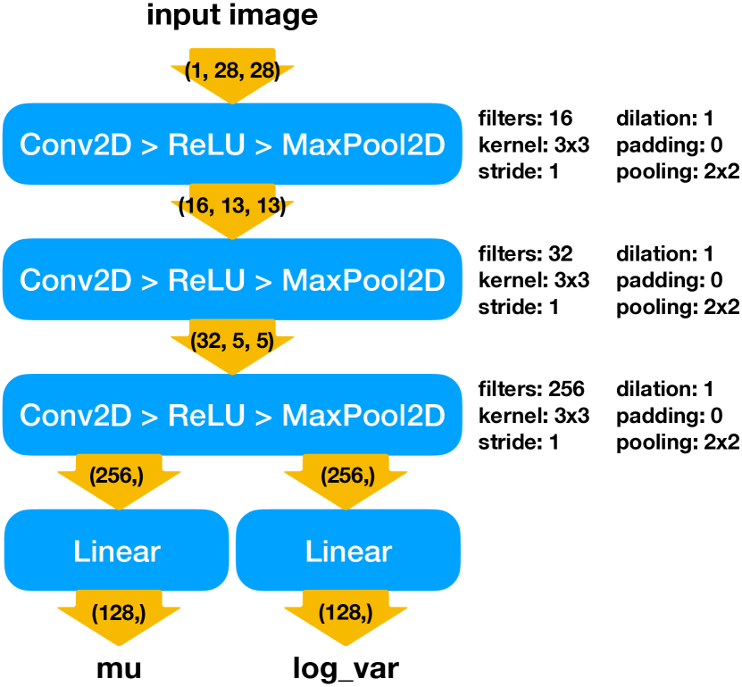
Refer to caption
(a) Encoder architecture
Refer to caption
(b) Decoder architecture
Figure 3: Autoencoder: architecture for the encoder and decoder

C.2 Creating the generators

The generators used in these numerical simulations were obtained as the decoders of trained VAEs. The MNIST database [3] of images was used for these simulations. The images of this database are grayscale 28×28282828\times 28 images of handwritten digits. Each network only used images corresponding to a single digit class. For this simulation, the digit class 111 was used in training the first VAE, for which there were 7877 images; 888 for the second VAE, for which there were 6825 images. For each network, the images were randomly partitioned into training, validation and test sets (70%, 15%, 15%, respectively). No image augmentations (e.g., random flips or random crops) were used. For both networks, the training batch size was 32, and the number of epochs used for training was 200. Early stopping was not used, as we found that the validation loss continued to decrease for the duration of training.

Both networks were variational auto-encoders (VAEs) whose encoders used 2D convolutional layers with max-pooling, and whose decoders used 2D transposed convolutions for image generation. The architectures for the encoder and the decoder are depicted in 3(a) and 3(b), respectively. The latent dimension for both VAEs was 128128128. Both VAEs assumed that the conditional distribution on the latent codes was Gaussian, as described in Variational Autoencoders. Both VAEs were trained using a modification of mini-batch stochastic gradient descent (SGD) [8] with a learning rate of 105superscript10510^{-5}, momentum of 0.90.90.9 and weight decay of 103superscript10310^{-3}, using the standard PyTorch implementation of SGD [22]. Results of the training are depicted in Figure 4. In particular, 4(a) for the VAE trained on 111s, and 4(b) for the VAE trained on 888s.

Example outputs from noisy latent codes obtained from the validation data are depicted in Figure 5. Specifically, this figure offers a comparison of true images from the validation set and their auto-encoded approximations. Validation images from the 111s dataset can be found in the left panel of 5(a), and their reconstructions in the right panel. Validation images from the 888s dataset can be found in the left panel of 5(b); their reconstructions in the right panel. The correspondence between the true image and the auto-encoded approximation is given according to the image’s row-column position in the grid.
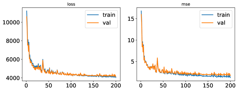
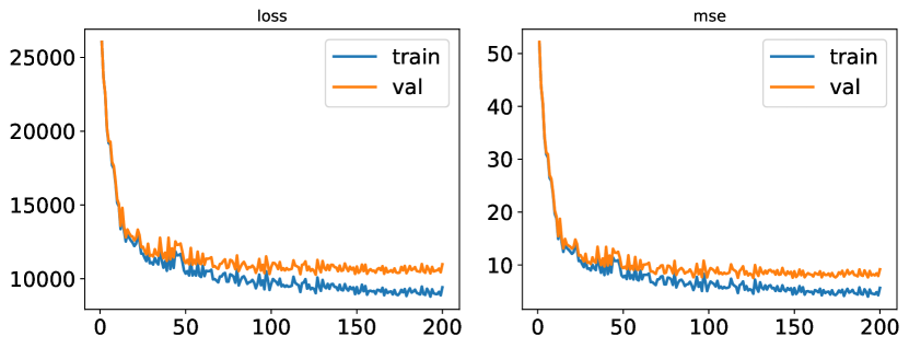
Refer to caption
(a) Loss & MSE for VAE trained on 111s.
Refer to caption
(b) Loss & MSE for VAE trained on 888s.
Figure 4: In each sub-figure, the left plot gives the average training and validation loss after each epoch; the right the training and validation MSE after each epoch.
Refer to caption
Refer to caption
(a) True and reconstructed images from the 111s VAE
Refer to caption
Refer to caption
(b) True and reconstructed images from the 888s VAE
Figure 5: Validation images and their reconstructions by each VAE. In each subfigure, true images from the validation data are shown in the left grid; their reconstruction by the decoder from codes that were partially corrupted are on the right.

C.3 Generative demixing numerical implementation

Generally, the trained encoder network can be interpreted as a map from an image to the encoder’s latent code for that image in the VAE’s latent space. The decoder can be interpreted as a mapping from the latent space back into the relevant space of natural images. In this way, we are able to use the decoder as a structural proxy corresponding to a low-dimensional representation for an image, just as one might use a particular convex strucutural proxy like the 1subscript1\ell_{1} ball to encode a sparse signal in the classical compressed sensing setting. For further intuition regarding this point we refer the reader to Introduction and [1, 9, 17].

The initial mixture b𝑏b for the demixing problem was obtained as described in (3). As a minor technical point, we note that the values of the resulting mixture b𝑏b were clipped to [0,1]01[0,1], as were those of the predicted mixture at each iteration of the recovery algorithm. We found that the presence of clipping had no apparent effect on recovery performance, but aided visual interpretation of the resulting images. The initial encodings w1(0),w8(0)128superscriptsubscript𝑤10superscriptsubscript𝑤80superscript128w_{1}^{(0)},w_{8}^{(0)}\in\mathbb{R}^{128} used by each VAE decoder 𝒟1,𝒟8subscript𝒟1subscript𝒟8\mathcal{D}_{1},\mathcal{D}_{8} were obtained for b𝑏b using the VAEs’ encoders 1,8subscript1subscript8\mathcal{E}_{1},\mathcal{E}_{8} and random noise:

wc(0)=c(b)+0.1ε,c{1,8},εiiid𝒩(0,1).formulae-sequencesuperscriptsubscript𝑤𝑐0subscript𝑐𝑏0.1𝜀𝑐18subscript𝜀𝑖iidsimilar-to𝒩01\displaystyle w_{c}^{(0)}=\mathcal{E}_{c}(b)+0.1\cdot\varepsilon,\qquad c\in\{1,8\},\varepsilon_{i}\overset{\text{iid}}{\sim}\mathcal{N}(0,1).

To solve the demixing problem numerically, the MSE loss of the difference between the predicted mixture and the true mixture was minimized using Adam [13] with a learning rate of 102superscript10210^{-2} for 100010001000 iterations using PyTorch [22]. Our proposed algorithm, using PyTorch-themed pseudo-code, is presented in Figure 6. For sake of clarity to the reader, we have removed some minor code-specific details, and have used suggestive variable names. The recovered image approximating x1subscript𝑥1x_{1} had an MSE of 1.591031.59superscript1031.59\cdot 10^{-3}; that for x8subscript𝑥8x_{8}, 7.481047.48superscript1047.48\cdot 10^{-4}; that for the mixture, 3.921043.92superscript1043.92\cdot 10^{-4}. A graphical depiction of the results appear in Figure 2 as Figures 1(a)2(d).

1for i in range(num_iter):
2 # compute de-mixed images from latent codes
3 demixed_1 = vae_1.decode(w_1)
4 demixed_8 = vae_8.decode(w_8)
5 # clear gradients from previous iteration
6 optimizer.zero_grad()
7 # obtain predicted mixture
8 mixture_pred = mixer(demixed_1, demixed_8)
9 # compute MSE loss between predicted and true mixture
10 loss = criterion(mixture_pred.view(1, -1), mixture.view(1, -1))
11 # back-propagate to compute gradients
12 loss.backward()
13 # update w_1 and w_8
14 optimizer.step()
Figure 6: PyTorch pseudo-code for implementing the demixing algorithm.
1# Establish Architecture
2Encoder #*$\leftarrow$*) GetEncoderArchitecture()
3Decoder #*$\leftarrow$*) GetDecoderArchitecture()
4AutoEncoder #*$\leftarrow$*) function(x, Encoder, Decoder):
5 xReconstructed #*$\leftarrow$*) Decoder(SampleFrom(Encoder(x)))
6 Return xReconstructed
7
8# Train VAEs
9TrainedDecoder0, TrainedEncoder0 #*$\leftarrow$*) MinibatchSGD(
10 Decoder,
11 Encoder,
12 TrainingData0,
13 ValidationData0,
14 VAELoss,
15 VAEOptimizationParameters,
16)
17TrainedDecoder1, TrainedEncoder1 #*$\leftarrow$*) MinibatchSGD(
18 Decoder,
19 Encoder,
20 TrainingData1,
21 ValidationData1,
22 VAELoss,
23 VAEOptimizationParameters,
24)
25
26# Demixing Algorithm
27x0 #*$\leftarrow$*) SampleFrom(TestData0)
28x1 #*$\leftarrow$*) SampleFrom(TestData1)
29A #*$\leftarrow$*) SampleFrom(NormalizedGaussianRandomMatrices)
30b #*$\leftarrow$*) Mult(A, x0) + x1
31w_init0, w_init1 #*$\leftarrow$*) ComputeInitialEncodings()
32DemixedImage0, DemixedImage1 #*$\leftarrow$*) RunDemixing(
33 w_init0,
34 w_init1,
35 TrainedDecoder0,
36 TrainedDecoder1,
37 MSELoss,
38 AdamOptimizer,
39 DemixOptimizationParameters,
40)
Figure 7: A pseudo-code meta-algorithm serving as roadmap for the numerics of this work.