On the Fairness of Causal Algorithmic Recourse

Abstract

Algorithmic fairness is typically studied from the perspective of predictions. Instead, here we investigate fairness from the perspective of recourse actions suggested to individuals to remedy an unfavourable classification. We propose two new fairness criteria at the group and individual level, which—unlike prior work on equalising the average group-wise distance from the decision boundary—explicitly account for causal relationships between features, thereby capturing downstream effects of recourse actions performed in the physical world. We explore how our criteria relate to others, such as counterfactual fairness, and show that fairness of recourse is complementary to fairness of prediction. We study theoretically and empirically how to enforce fair causal recourse by altering the classifier and perform a case study on the Adult dataset. Finally, we discuss whether fairness violations in the data generating process revealed by our criteria may be better addressed by societal interventions as opposed to constraints on the classifier.

1 Introduction

Algorithmic fairness is concerned with uncovering and correcting for potentially discriminatory behavior of automated decision making systems (Dwork et al. 2012; Zemel et al. 2013; Hardt, Price, and Srebro 2016; Chouldechova 2017). Given a dataset comprising individuals from multiple legally protected groups (defined, e.g., based on age, sex, or ethnicity), and a binary classifier trained to predict a decision (e.g., whether they were approved for a credit card), most approaches to algorithmic fairness seek to quantify the level of unfairness according to a pre-defined (statistical or causal) criterion, and then aim to correct it by altering the classifier. This notion of predictive fairness typically considers the dataset as fixed, and thus the individuals as unalterable.

Algorithmic recourse, on the other hand, is concerned with offering recommendations to individuals, who were unfavourably treated by a decision-making system, to overcome their adverse situation (Joshi et al. 2019; Ustun, Spangher, and Liu 2019; Sharma, Henderson, and Ghosh 2019; Mahajan, Tan, and Sharma 2019; Mothilal, Sharma, and Tan 2020; Venkatasubramanian and Alfano 2020; Karimi et al. 2020c, b; Karimi, Schölkopf, and Valera 2021; Upadhyay, Joshi, and Lakkaraju 2021). For a given classifier and a negatively-classified individual, algorithmic recourse aims to identify which changes the individual could perform to flip the decision. Contrary to predictive fairness, recourse thus considers the classifier as fixed but ascribes agency to the individual.

Figure 1: Example demonstrating the difference between fair prediction and fair recourse: here, only the variance of (centered income) $X$ differs across two protected groups $A\in\{0,1\}$, while the true and predicted label (whether an individual is approved for a credit card) are determined by $\mathop{\mathrm{sign}}(X)$. This scenario would be considered fair from the perspective of prediction, but the cost of recourse (here, the distance to the decision boundary, set at $X=0$) is much larger for individuals in the blue group with $A=0$.

Within machine learning (ML), fairness and recourse have mostly been considered in isolation and viewed as separate problems. While recourse has been investigated in the presence of protected attributes—e.g., by comparing recourse actions (flipsets) suggested to otherwise similar male and female individuals (Ustun, Spangher, and Liu 2019), or comparing the aggregated cost of recourse (burden) across different protected groups (Sharma, Henderson, and Ghosh 2019)—its relation to fairness has only been studied informally, in the sense that differences in recourse have typically been understood as proxies of predictive unfairness (Karimi et al. 2020a). However, as we argue in the present work, recourse actually constitutes an interesting fairness criterion in its own right as it allows for the notions of agency and effort to be integrated into the study of fairness.

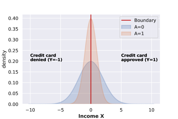
In fact, discriminatory recourse does not imply predictive unfairness (and is not implied by it either). To see this, consider the data shown in Fig. 1. Suppose the feature $X$ represents the (centered) income of an individual from one of two sub-groups $A\in\{0,1\}$, distributed as $\mathcal{N}(0,1)$ and $\mathcal{N}(0,4)$, i.e., only the variances differ. Now consider a binary classifier $h(X)=\text{sign}(X)$ which perfectly predicts whether the individual is approved for a credit card (the true label $Y$) (Barocas, Selbst, and Raghavan 2020). While this scenario satisfies several predictive fairness criteria (e.g., demographic parity, equalised odds, calibration), the required increase in income for negatively-classified individuals to be approved for a credit card (i.e., the effort required to achieve recourse) is much larger for the higher variance group. If individuals from one protected group need to work harder than “similar” ones from another group to achieve the same goal, this violates the concept of equal opportunity, a notion aiming for people to operate on a level playing field (Arneson 2015). However, this type of unfairness is not captured by predictive notions which—in only distinguishing between (unalterable) worthy or unworthy individuals—do not consider the possibility for individuals to deliberately improve their situation by means of changes or interventions.

In this vein, Gupta et al. (2019) recently introduced Equalizing Recourse, the first recourse-based and prediction-independent notion of fairness in ML. They propose to measure recourse fairness in terms of the average group-wise distance to the decision boundary for those getting a bad outcome, and show that this can be calibrated during classifier training. However, this formulation ignores that recourse is fundamentally a causal problem since actions performed by individuals in the real-world to change their situation may have downstream effects (Mahajan, Tan, and Sharma 2019; Karimi, Schölkopf, and Valera 2021; Karimi et al. 2020c; Mothilal, Sharma, and Tan 2020), cf. also (Barocas, Selbst, and Raghavan 2020; Wachter, Mittelstadt, and Russell 2017; Ustun, Spangher, and Liu 2019). By not reasoning about causal relations between features, the distance-based approach (i) does not accurately reflect the true (differences in) recourse cost, and (ii) is restricted to the classical prediction-centered approach of changing the classifier to address discriminatory recourse.

In the present work, we address both of these limitations. First, by extending the idea of Equalizing Recourse to the minimal intervention-based framework of recourse (Karimi, Schölkopf, and Valera 2021), we introduce causal notions of fair recourse which capture the true differences in recourse cost more faithfully if features are not independently manipulable, as is generally the case. Second, we argue that a causal model of the data generating process opens up a new route to fairness via societal interventions in the form of changes to the underlying system. Such societal interventions may reflect common policies like subgroup-specific subsidies or tax breaks. We highlight the following contributions:

• we introduce a causal version (Defn. 3.1) of Equalizing Recourse, as well as a stronger (Prop. 3.3) individual-level criterion (Defn. 3.2) which we argue is more appropriate;

• we provide the first formal study of the relation between fair prediction and fair recourse, and show that they are complementary notions which do not imply each other (Prop. 3.4);

• we establish sufficient conditions that allow for individually-fair causal recourse (Prop. 3.6);

• we evaluate different fair recourse metrics for several classifiers (§ 4.1), verify our main results, and demonstrate that non-causal metrics misrepresent recourse unfairness;

• in a case study on the Adult dataset, we detect recourse discrimination at the group and individual level (§ 4.2), demonstrating its relevance for real world settings;

• we propose societal interventions as an alternative to altering a classifier to address unfairness (§ 5).

2 Preliminaries & Background

Notation.

Let the random vector $\mathbf{X}=(X_{1},...,X_{n})$ taking values $\mathbf{x}=(x_{1},...,x_{n})\in\mathcal{X}=\mathcal{X}_{1}\times...\times\mathcal{X}_{n}\subseteq\mathbb{R}^{n}$ denote observed (non-protected) features. Let the random variable $A$ taking values $a\in\mathcal{A}=\{1,\ldots,K\}$ for some $K\in\mathbb{Z}_{>1}$ denote a (legally) protected attribute/feature indicating which group each individual belongs to (based, e.g., on her age, sex, ethnicity, religion, etc). And let $h:\mathcal{X}\rightarrow\mathcal{Y}$ be a given binary classifier with $Y\in\mathcal{Y}=\{\pm 1\}$ denoting the ground truth label (e.g., whether her credit card was approved). We observe a dataset $\mathcal{D}=\{\mathbf{v}^{i}\}_{i=1}^{N}$ of i.i.d. observations of the random variable $\mathbf{V}=(\mathbf{X},A)$ with $\mathbf{v}^{i}:=(\mathbf{x}^{i},a^{i})$.

Counterfactual Explanations.

A common framework for explaining decisions made by (black-box) ML models is that of counterfactual explanations (CE; Wachter, Mittelstadt, and Russell 2017). A CE is a closest feature vector on the other side of the decision boundary. Given a distance $d:\mathcal{X}\times\mathcal{X}\rightarrow\mathbb{R}^{+}$, a CE for an individual $\mathbf{x}^{\texttt{F}}$ who obtained an unfavourable prediction, $h(\mathbf{x}^{\texttt{F}})=-1$, is defined as a solution to:

$$\min_{\mathbf{x}\in\mathcal{X}}\,d(\mathbf{x},\mathbf{x}^{\texttt{F}})\quad\quad\text{subject to}\quad\quad h(\mathbf{x})=1.$$ (1)

While CEs are useful to understand the behaviour of a classifier, they do not generally lead to actionable recommendations: they inform an individual of where she should be to obtain a more favourable prediction, but they may not suggest feasible changes she could perform to get there.

(a) IMF assumption

(b) Causal view

Figure 2: (a) The framework underlying counterfactual explanations and distance-based recourse treats $X_{i}$ as independently manipulable features (IMF). In a fairness context, this means that the $X_{i}$ may depend on the protected attribute $A$ (and potentially other unobserved factors) but do not causally influence each other. (b) The present work considers a generalisation the IMF assumption by allowing for causal influences between the $X_{i}$, thus modeling the downstream effects of changing some features on others. This causal approach allows us to more accurately quantify recourse unfairness in real-world settings where the IMF assumption is typically violated. It also provides a framework for studying alternative routes to achieve fair recourse beyond changing the classifier.

Recourse with Independently-Manipulable Features.

Ustun, Spangher, and Liu (2019) refer to a person’s ability to change the decision of a model by altering actionable variables as recourse and propose to solve

$$\min_{\bm{\delta}\in\mathcal{F}(\mathbf{x}^{\texttt{F}})}\,c(\bm{\delta};\mathbf{x}^{\texttt{F}})\quad\text{subject to}\quad h(\mathbf{x}^{\texttt{F}}+\bm{\delta})=1$$ (2)

where $\mathcal{F}(\mathbf{x}^{\texttt{F}})$ is a set of feasible change vectors and $c(\cdot;\mathbf{x}^{\texttt{F}})$ is a cost function defined over these actions, both of which may depend on the individual. As pointed out by Karimi, Schölkopf, and Valera (2021), (2) implicitly treats features as manipulable independently of each other (see Fig. 2(a)) and does not account for causal relations that may exist between them (see Fig. 2(b)): while allowing feasibility constraints on actions, variables which are not acted-upon ($\delta_{i}=0$) are assumed to remain unchanged. We refer to this as the independently-manipulable features (IMF) assumption. While the IMF-view may be appropriate when only analysing the behaviour of a classifier, it falls short of capturing effects of interventions performed in the real world, as is the case in actionable recourse; e.g., an increase in income will likely also positively affect the individual’s savings balance. As a consequence, (2) only guarantees recourse if the acted-upon variables have no causal effect on the remaining variables (Karimi, Schölkopf, and Valera 2021).

Structural Causal Models.

A structural causal model (SCM) (Pearl 2009; Peters, Janzing, and Schölkopf 2017) over observed variables $\mathbf{V}=\{V_{i}\}_{i=1}^{n}$ is a pair $\mathcal{M}=(\mathbf{S},\mathbb{P}_{\mathbf{U}})$, where the structural equations $\mathbf{S}$ are a set of assignments $\mathbf{S}=\{V_{i}:=f_{i}(\text{PA}_{i},U_{i})\}_{i=1}^{n}$, which compute each $V_{i}$ as a deterministic function $f_{i}$ of its direct causes (causal parents) $\text{PA}_{i}\subseteq\mathbf{V}\setminus V_{i}$ and an unobserved variable $U_{i}$. In this work, we make the common assumption that the distribution $\mathbb{P}_{\mathbf{U}}$ factorises over the latent $\mathbf{U}=\{U_{i}\}_{i=1}^{n}$, meaning that there is no unobserved confounding (causal sufficiency). If the causal graph $\mathcal{G}$ associated with $\mathcal{M}$ (obtained by drawing a directed edge from each variable in $\text{PA}_{i}$ to $V_{i}$, see Fig. 2 for examples) is acyclic, $\mathcal{M}$ induces a unique “observational” distribution over $\mathbf{V}$, defined as the push forward of $\mathbb{P}_{\mathbf{U}}$ via $\mathbf{S}$.

SCMs can be used to model the effect of interventions: external manipulations to the system that change the generative process (i.e., the structural assignments) of a subset of variables $\mathbf{V}_{\mathcal{I}}\subseteq\mathbf{V}$, e.g., by fixing their value to a constant $\bm{\theta}_{\mathcal{I}}$. Such (atomic) interventions are denoted using Pearl’s $do$-operator by $do(\mathbf{V}_{\mathcal{I}}:=\bm{\theta}_{\mathcal{I}})$, or $do(\bm{\theta}_{\mathcal{I}})$ for short. Interventional distributions are obtained from $\mathcal{M}$ by replacing the structural equations $\{V_{i}:=f_{i}(\text{PA}_{i},U_{i})\}_{i\in\mathcal{I}}$ by their new assignments $\{V_{i}:=\theta_{i}\}_{i\in\mathcal{I}}$ to obtain the modified structural equations $\mathbf{S}^{do(\bm{\theta}_{\mathcal{I}})}$ and then computing the distribution induced by the interventional SCM $\mathcal{M}^{do(\bm{\theta}_{\mathcal{I}})}=(\mathbf{S}^{do(\bm{\theta}_{\mathcal{I}})},\mathbb{P}_{\mathbf{U}})$, i.e., the push-forward of $\mathbb{P}_{\mathbf{U}}$ via $\mathbf{S}^{do(\bm{\theta}_{\mathcal{I}})}$.

Similarly, SCMs allow reasoning about (structural) counterfactuals: statements about interventions performed in a hypothetical world where all unobserved noise terms $\mathbf{U}$ are kept unchanged and fixed to their factual value $\mathbf{u}^{\texttt{F}}$. The counterfactual distribution for a hypothetical intervention $do(\bm{\theta}_{\mathcal{I}})$ given a factual observation $\mathbf{v}^{\texttt{F}}$, denoted $\mathbf{v}_{\bm{\theta}_{\mathcal{I}}}(\mathbf{u}^{\texttt{F}})$, can be obtained from $\mathcal{M}$ using a three step procedure: first, inferring the posterior distribution over the unobserved variables $\mathbb{P}_{\mathbf{U}|\mathbf{v}^{\texttt{F}}}$ (abduction); second, replacing some of the structural equations as in the interventional case (action); third, computing the distribution induced by the counterfactual SCM $\mathcal{M}^{do(\bm{\theta}_{\mathcal{I}})|\mathbf{v}^{\texttt{F}}}=(\mathbf{S}^{do(\bm{\theta}_{\mathcal{I}})},\mathbb{P}_{\mathbf{U}|\mathbf{v}^{\texttt{F}}})$ (prediction).

Causal Recourse.

To capture causal relations between features, Karimi, Schölkopf, and Valera (2021) propose to approach the actionable recourse task within the framework of SCMs and to shift the focus from nearest CEs to minimal interventions, leading to the optimisation problem

$$\min_{\bm{\theta}_{\mathcal{I}}\in\mathcal{F}(\mathbf{x}^{\texttt{F}})}\,c(\bm{\theta}_{\mathcal{I}};\mathbf{x}^{\texttt{F}})\quad\text{subj.\ to}\quad h(\mathbf{x}_{\bm{\theta}_{\mathcal{I}}}(\mathbf{u}^{\texttt{F}}))=1,$$ (3)

where $\mathbf{x}_{\bm{\theta}_{\mathcal{I}}}(\mathbf{u}^{\texttt{F}})$ denotes the “counterfactual twin” of $\mathbf{x}^{\texttt{F}}$ had $\mathbf{X}_{\mathcal{I}}$ been $\bm{\theta}_{\mathcal{I}}$. In practice, the SCM is unknown and needs to be inferred from data based on additional (domain-specific) assumptions, leading to probabilistic versions of (3) which aim to find actions that achieve recourse with high probability (Karimi et al. 2020c). If the IMF assumptions holds (i.e., the set of descendants of all actionable variables is empty), then (3) reduces to IMF recourse (2) as a special case.

Algorithmic and Counterfactual Fairness.

While there are many statistical notions of fairness (Zafar et al. 2017a, b), these are sometimes mutually incompatible (Chouldechova 2017), and it has been argued that discrimination, at its heart, corresponds to a (direct or indirect) causal influence of a protected attribute on the prediction, thus making fairness a fundamentally causal problem (Kilbertus et al. 2017; Russell et al. 2017; Loftus et al. 2018; Zhang and Bareinboim 2018a, b; Nabi and Shpitser 2018; Nabi, Malinsky, and Shpitser 2019; Chiappa 2019; Salimi et al. 2019; Wu et al. 2019). Of particular interest to our work is the notion of counterfactual fairness introduced by Kusner et al. (2017) which calls a (probabilistic) classifier $h$ over $\mathbf{V}=\mathbf{X}\cup A$ counterfactually fair if it satisfies

$$h(\mathbf{v}^{\texttt{F}})=h(\mathbf{v}_{a}(\mathbf{u}^{\texttt{F}})),\forall a\in\mathcal{A},\mathbf{v}^{\texttt{F}}=(\mathbf{x}^{\texttt{F}},a^{\texttt{F}})\in\mathcal{X}\times\mathcal{A},$$

where $\mathbf{v}_{a}(\mathbf{u}^{\texttt{F}})$ denotes the “counterfactual twin” of $\mathbf{v}^{\texttt{F}}$ had the attribute been $a$ instead of $a^{\texttt{F}}$.

Equalizing Recourse Across Groups.

The main focus of this paper is the fairness of recourse actions which, to the best of our knowledge, was studied for the first time by Gupta et al. (2019). They advocate for equalizing the average cost of recourse across protected groups and to incorporate this as a constraint when training a classifier. Taking a distance-based approach in line with CEs, they define the cost of recourse for $\mathbf{x}^{\texttt{F}}$ with $h(\mathbf{x}^{\texttt{F}})=-1$ as the minimum achieved in (1):

$$r^{\textsc{imf}}(\mathbf{x}^{\texttt{F}})=\min_{\mathbf{x}\in\mathcal{X}}\,d(\mathbf{x}^{\texttt{F}},\mathbf{x})\quad\text{subj.\ to}\quad h(\mathbf{x})=1,$$ (4)

which is equivalent to IMF-recourse (2) if $c(\bm{\delta};\mathbf{x}^{\texttt{F}})=d(\mathbf{x}^{\texttt{F}}+\bm{\delta},\mathbf{x}^{\texttt{F}})$ is chosen as cost function. Defining the protected subgroups, $G_{a}=\{\mathbf{v}^{i}\in\mathcal{D}:a^{i}=a\}$, and $G_{a}^{-}=\{\mathbf{v}\in G_{a}:h(\mathbf{v})=-1\}$, the group-level cost of recourse (here, the average distance to the decision boundary) is then given by,

$$\textstyle r^{\textsc{imf}}(G_{a}^{-})=\frac{1}{|G_{a}^{-}|}\sum_{\mathbf{v}^{i}\in G_{a}^{-}}r^{\textsc{imf}}(\mathbf{x}^{i}).$$ (5)

The idea of Equalizing Recourse across groups (Gupta et al. 2019) can then be summarised as follows.

Definition 2.1 (Group-level fair IMF-recourse, from (Gupta et al. 2019)).

The group-level unfairness of recourse with independently-manipulable features (IMF) for a dataset $\mathcal{D}$, classifier $h$, and distance metric $d$ is:

$$\Delta_{\mathbf{\mathrm{dist}}}(\mathcal{D},h,d):=\max_{a,a^{\prime}\in\mathcal{A}}\left|r^{\textsc{imf}}(G_{a}^{-})-r^{\textsc{imf}}(G_{a^{\prime}}^{-})\right|.$$

Recourse for $(\mathcal{D},h,d)$ is “group IMF-fair” if $\Delta_{\mathbf{\mathrm{dist}}}=0$.

3 Fair Causal Recourse

Since Defn. 2.1 rests on the IMF assumption, it ignores causal relationships between variables, fails to account for downstream effects of actions on other relevant features, and thus generally incorrectly estimates the true cost of recourse. We argue that recourse-based fairness considerations should rest on a causal model that captures the effect of interventions performed in the physical world where features are often causally related to each other. We therefore consider an SCM $\mathcal{M}$ over $\mathbf{V}=(\mathbf{X},A)$ to model causal relationships between the protected attribute and the remaining features.

3.1 Group-Level Fair Causal Recourse

Defn. 2.1 can be adapted to the causal (CAU) recourse framework (3) by replacing the minimum distance in (4) with the cost of recourse within a causal model, i.e., the minimum achieved in (3):

$$r^{\textsc{cau}}(\mathbf{v}^{\texttt{F}})=\min_{\bm{\theta}_{\mathcal{I}}\in\Theta(\mathbf{v}^{\texttt{F}})}\,c(\bm{\theta}_{\mathcal{I}};\mathbf{v}^{\texttt{F}})\quad\text{subj.\ to}\quad h(\mathbf{v}_{\bm{\theta}_{\mathcal{I}}}(\mathbf{u}^{\texttt{F}}))=1,$$

where we recall that the constraint $h(\mathbf{v}_{\bm{\theta}_{\mathcal{I}}}(\mathbf{u}^{\texttt{F}}))=1$ ensures that the counterfactual twin of $\mathbf{v}^{\texttt{F}}$ in $\mathcal{M}$ falls on the favourable side of the classifier. Let $r^{\textsc{cau}}(G_{a}^{-})$ be the average of $r^{\textsc{cau}}(\mathbf{v}^{\texttt{F}})$ across $G_{a}^{-}$, analogously to (5). We can then define group-level fair causal recourse as follows.

Definition 3.1 (Group-level fair causal recourse).

The group-level unfairness of causal (CAU) recourse for a dataset $\mathcal{D}$, classifier $h$, and cost function $c$ w.r.t. an SCM $\mathcal{M}$ is given by:

$$\Delta_{\mathbf{\mathrm{cost}}}(\mathcal{D},h,c,\mathcal{M}):=\max_{a,a^{\prime}\in\mathcal{A}}\left|r^{\textsc{cau}}(G_{a}^{-})-r^{\textsc{cau}}(G_{a^{\prime}}^{-})\right|.$$

Recourse for $(\mathcal{D},h,c,\mathcal{M})$ is “group CAU-fair” if $\Delta_{\mathbf{\mathrm{cost}}}=0$.

While Defn. 2.1 is agnostic to the (causal) generative process of the data (note the absence of a reference SCM $\mathcal{M}$ from Defn. 2.1),  Defn. 3.1 takes causal relationships between features into account when calculating the cost of recourse. It thus captures the effect of actions and the necessary cost of recourse more faithfully when the IMF-assumption is violated, as is realistic for most applications.

A shortcoming of both Defns. 2.1 and 3.1 is that they are group-level definitions, i.e., they only consider the average cost of recourse across all individuals sharing the same protected attribute. However, it has been argued from causal (Chiappa 2019; Wu et al. 2019) and non-causal (Dwork et al. 2012) perspectives that fairness is fundamentally an individual-level concept: group-level fairness still allows for unfairness at the level of the individual, provided that positive and negative discrimination cancel out across the group. This is one motivation behind counterfactual fairness (Kusner et al. 2017): a decision is considered fair at the individual level if it would not have changed, had the individual belonged to a different protected group.

3.2 Individually Fair Causal Recourse

Inspired by counterfactual fairness (Kusner et al. 2017), we propose that (causal) recourse may be considered fair at the level of the individual if the cost of recourse would have been the same had the individual belonged to a different protected group, i.e., under a counterfactual change to $A$.

Definition 3.2 (Individually fair causal recourse).

The individual-level unfairness of causal recourse for a dataset $\mathcal{D}$, classifier $h$, and cost function $c$ w.r.t. an SCM $\mathcal{M}$ is

$$\Delta_{\mathrm{ind}}(\mathcal{D},h,c,\mathcal{M}):=\max_{a\in\mathcal{A};\mathbf{v}^{\texttt{F}}\in\mathcal{D}}\left|r^{\textsc{cau}}(\mathbf{v}^{\texttt{F}})-r^{\textsc{cau}}(\mathbf{v}_{a}(\mathbf{u}^{\texttt{F}}))\right|$$

Recourse is “individually CAU-fair” if $\Delta_{\mathrm{ind}}=0$.

This is a stronger notion in the sense that it is possible to satisfy both group IMF-fair (Defn. 2.1) and group CAU-fair recourse (Defn. 3.1), without satisfying Defn. 3.2:

Proposition 3.3.

Neither of the group-level notions of fair recourse (Defn. 2.1 and Defn. 3.1) are sufficient conditions for individually CAU-fair recourse (Defn. 3.2), i.e.,

Group IMF-fair $$\centernot\implies\text{Individually CAU-fair}.$$

Group CAU-fair $$\centernot\implies\text{Individually CAU-fair}.$$

Proof.

A counterexample is given by the following combination of SCM and classifier

$$A :=U_{A},$$

$$X :=AU_{X}+(1-A)(1-U_{X}),$$

$$U_{A},U_{X} \sim\mathrm{Bernoulli}(0.5),$$

$$Y :=h(X)=\mathop{\mathrm{sign}}(X-0.5).$$

We have $\mathbb{P}_{X|A=0}=\mathbb{P}_{X|A=1}=\mathrm{Bern}(0.5)$, so the distance to the boundary at $X=0.5$ is the same across groups. The criterion for “group IMF-fair” recourse (Defn. 2.1) is thus satisfied.

Since protected attributes are generally immutable (thus making any recourse actions involving changes to $A$ infeasible) and since there is only a single feature in this example (so that causal downstream effects on descendant features can be ignored), the distance between the factual and counterfactual value of $X$ is a reasonable choice of cost function also for causal recourse. In this case, $(\mathcal{D},h,\mathcal{M})$ also satisfies group-level CAU-fair recourse (Defn. 3.1).

However, for all $\mathbf{v}^{\texttt{F}}=(x^{\texttt{F}},a^{\texttt{F}})$ and any $a\neq a^{\texttt{F}}$, we have $h(x^{\texttt{F}})\neq h(x_{a}(u_{X}^{\texttt{F}}))=1-h(x^{\texttt{F}})$, so it is maximally unfair at the individual level: for any individual, the cost of recourse would have been zero had the protected attribute been different, as the prediction would have flipped. ∎

3.3 Relation to Counterfactual Fairness

The classifier $h$ used in the proof of Prop. 3.3 is not counterfactually fair. This suggests to investigate their relation more closely: does a counterfactually fair classifier imply fair (causal) recourse? The answer is no.

Proposition 3.4.

Counterfactual fairness is insufficient for any of the three notions of fair recourse:

$$h\,\,\text{counterfactually fair} \centernot\implies\text{Group IMF-fair}$$

$$h\,\,\text{counterfactually fair} \centernot\implies\text{Group CAU-fair}$$

$$h\,\,\text{counterfactually fair} \centernot\implies\text{Individually CAU-fair}$$

Proof.

A counterexample is given by the following combination of SCM and classifier:

$$A :=U_{A}, U_{A} \sim\text{Bernoulli}(0.5),$$ (6)

$$X :=(2-A)U_{X}, U_{X} \sim\mathcal{N}(0,1),$$

$$Y :=h(X)=\mathop{\mathrm{sign}}(X)$$

which we used to generate Fig. 1. As $\mathop{\mathrm{sign}}(X)=\mathop{\mathrm{sign}}(U_{X})$, and $U_{X}$ is assumed fixed when reasoning about a counterfactual change of $A$, $h$ is counterfactually fair.

However, $\mathbb{P}_{X|A=0}=\mathcal{N}(0,4)$ and $\mathbb{P}_{X|A=1}=\mathcal{N}(0,1)$, so the distance to the boundary (which is a reasonable cost for cau-recourse in this one-variable toy example) differs at the group level. Moreover, $X$ either doubles or halves when counterfactually changing $A$. ∎

Remark 3.5.

An important characteristic of the counterexample used in the proof of Prop. 3.4 is that $h$ is deterministic, which makes it possible that $h$ is counterfactually fair, even though it depends on a descendant of $A$. This is generally not be the case if $h$ is probabilistic (e.g., a logistic regression), $h:\mathcal{X}\rightarrow[0,1]$, so that the probability of a positive classification decreases with the distance from the decision boundary.

(a) IMF

(b) CAU

(c) Adult

Figure 3: (a) & (b) Causal graphs used in § 4.1. (c) The (assumed) causal graph (from Chiappa (2019); Nabi and Shpitser (2018)) used for the Adult dataset (Lichman et al. 2013); $\mathbf{A}$ denotes the three protected attributes {sex, age, nationality}; $\mathbf{M}$ denotes {marital status, education level}; and $\mathbf{W}$ corresponds to {working class, occupation, hrs per week}. Here, we show the coarse-grained causal graph for simplicity. In practice, we model each node separately. For example, the single arrow from $A$ to $M$ actually corresponds to six directed edges, one from each feature in $\mathbf{A}$ to each feature in $\mathbf{M}$.

3.4 Achieving Fair Causal Recourse

Constrained Optimisation.

A first approach is to explicitly take constraints on the (group or individual level) fairness of causal recourse into account when training a classifier, as implemented for non-causal recourse under the IMF assumption by Gupta et al. (2019). Herein we can control the potential trade-off between accuracy and fairness with a hyperparameter. However, the optimisation problem in (3) involves optimising over the combinatorial space of intervention targets $\mathcal{I}\subseteq\{1,...,n\}$, so it is unclear whether fairness of causal recourse may easily be included as a differentiable constraint.

Restricting the Classifier Inputs.

An approach that only requires qualitative knowledge in form of the causal graph (but not a fully-specified SCM), is to restrict the set of input features to the classifier to only contain non-descendants of the protected attribute. In this case, and subject to some additional assumptions stated in more detail below, individually fair causal recourse can be guaranteed.

Proposition 3.6.

Assume $h$ only depends on a subset $\tilde{\mathbf{X}}\subseteq\mathbf{V}\setminus(A\cup\mathrm{desc}(A))$ which are non-descendants of $A$ in $\mathcal{M}$; and that the set of feasible actions and their cost remain the same under a counterfactual change of $A$, $\mathcal{F}(\mathbf{v}^{\texttt{F}})=\mathcal{F}(\mathbf{v}_{a}(\mathbf{u}^{\texttt{F}}))$ and $c(\cdot\,;\mathbf{v}^{\texttt{F}})=c(\cdot\,;\mathbf{v}_{a}(\mathbf{u}^{\texttt{F}}))$ $\forall a\in\mathcal{A},\mathbf{v}^{\texttt{F}}\in\mathcal{D}$. Then recourse for $(\mathcal{D},h,c,\mathcal{M})$ is “individually CAU-fair”.

Proof.

According to Defn. 3.2, it suffices to show that

$$r^{\textsc{cau}}(\mathbf{v}^{\texttt{F}})=r^{\textsc{cau}}(\mathbf{v}_{a}(\mathbf{u}^{\texttt{F}})),\quad\quad\forall a\in\mathcal{A},\mathbf{v}^{\texttt{F}}\in\mathcal{D}.$$ (7)

Substituting our assumptions in the definition of $r^{\textsc{cau}}$ from § 3.1, we obtain:

$$r^{\textsc{cau}}(\mathbf{v}^{\texttt{F}}) =\min_{\bm{\theta}_{\mathcal{I}}\in\mathcal{F}(\mathbf{v}^{\texttt{F}})}\,c(\bm{\theta}_{\mathcal{I}};\mathbf{v}^{\texttt{F}})\quad\text{s.t.}\quad h(\tilde{\mathbf{x}}_{\bm{\theta}_{\mathcal{I}}}(\mathbf{u}^{\texttt{F}}))=1,$$

$$r^{\textsc{cau}}(\mathbf{v}_{a}(\mathbf{u}^{\texttt{F}})) =\min_{\bm{\theta}_{\mathcal{I}}\in\mathcal{F}(\mathbf{v}^{\texttt{F}})}\,c(\bm{\theta}_{\mathcal{I}};\mathbf{v}^{\texttt{F}})\quad\text{s.t.}\quad h(\tilde{\mathbf{x}}_{\bm{\theta}_{\mathcal{I}},a}(\mathbf{u}^{\texttt{F}}))=1.$$

It remains to show that

$$\tilde{\mathbf{x}}_{\bm{\theta}_{\mathcal{I}},a}(\mathbf{u}^{\texttt{F}})=\tilde{\mathbf{x}}_{\bm{\theta}_{\mathcal{I}}}(\mathbf{u}^{\texttt{F}}),\quad\quad\forall\bm{\theta}_{\mathcal{I}}\in\mathcal{F}(\mathbf{v}^{\texttt{F}}),a\in\mathcal{A}$$

which follows from applying do-calculus (Pearl 2009) since $\tilde{\mathbf{X}}$ does not contain any descendants of $A$ by assumption, and is thus not influenced by counterfactual changes to $A$. ∎

The assumption of Prop. 3.6 that both the set of feasible actions $\mathcal{F}(\mathbf{v}^{\texttt{F}})$ and the cost function $c(\cdot\,;\mathbf{v}^{\texttt{F}})$ remain the same under a counterfactual change to the protected attribute may not always hold. For example, if a protected group were precluded (by law) or discouraged from performing certain recourse actions such as taking on a particular job or applying for a certification, that would constitute such a violation due to a separate source of discrimination.

Moreover, since protected attributes usually represent socio-demographic features (e.g., age, gender, ethnicity, etc), they often appear as root nodes in the causal graph and have downstream effects on numerous other features. Forcing the classifier to only consider non-descendants of $A$ as inputs, as in Prop. 3.6, can therefore lead to a drop in accuracy which can be a restriction (Wu, Zhang, and Wu 2019).

Abduction / Representation Learning.

We have shown that considering only non-descendants of $A$ is a way to achieve individually CAU-fair recourse. In particular, this also applies to the unobserved variables $\mathbf{U}$ which are, by definition, not descendants of any observed variables. This suggests to use $U_{i}$ in place of any descendants $X_{i}$ of $A$ when training the classifier—in a way, $U_{i}$ can be seen as a “fair representation” of $X_{i}$ since it is an exogenous component that is not due to $A$. However, as $\mathbf{U}$ is unobserved, it needs to be inferred from the observed $\mathbf{v}^{\texttt{F}}$, corresponding to the abduction step of counterfactual reasoning. Great care needs to be taken in learning such a representation in terms of the (fair) background variables as (untestable) counterfactual assumptions are required (Kusner et al. 2017, § 4.1).

Classifier	GT labels from linear log. reg. $\rightarrow$ using linear kernel / linear log. reg.												GT labels from nonlinear log. reg. $\rightarrow$ using polynomial kernel / nonlinear log. reg.
	IMF				CAU-LIN				CAU-ANM				IMF				CAU-LIN				CAU-ANM
	Acc	$\Delta_{\textbf{dist}}$	$\Delta_{\textbf{cost}}$	$\Delta_{\textbf{ind}}$	Acc	$\Delta_{\textbf{dist}}$	$\Delta_{\textbf{cost}}$	$\Delta_{\textbf{ind}}$	Acc	$\Delta_{\textbf{dist}}$	$\Delta_{\textbf{cost}}$	$\Delta_{\textbf{ind}}$	Acc	$\Delta_{\textbf{dist}}$	$\Delta_{\textbf{cost}}$	$\Delta_{\textbf{ind}}$	Acc	$\Delta_{\textbf{dist}}$	$\Delta_{\textbf{cost}}$	$\Delta_{\textbf{ind}}$	Acc	$\Delta_{\textbf{dist}}$	$\Delta_{\textbf{cost}}$	$\Delta_{\textbf{ind}}$
SVM$(\mathbf{X},A)$	86.5	0.96	0.40	1.63	89.5	1.18	0.44	2.11	88.2	0.65	0.27	2.32	90.8	0.05	0.00	1.09	91.1	0.07	0.03	1.06	90.6	0.04	0.03	1.40
LR$(\mathbf{X},A)$	86.7	0.48	0.50	1.91	89.5	0.63	0.53	2.11	87.7	0.40	0.34	2.32	90.5	0.08	0.03	1.06	90.6	0.09	0.01	1.00	90.6	0.19	0.22	1.28
SVM$(\mathbf{X})$	86.4	0.99	0.42	1.80	89.4	1.61	0.61	2.11	88.0	0.56	0.29	2.79	91.4	0.13	0.00	0.92	91.0	0.17	0.08	1.09	91.0	0.02	0.03	1.64
LR$(\mathbf{X})$	86.6	0.47	0.53	1.80	89.5	0.64	0.57	2.11	87.7	0.41	0.43	2.79	91.0	0.12	0.03	1.01	90.6	0.13	0.10	1.65	90.9	0.08	0.06	1.66
FairSVM$(\mathbf{X},A)$	68.1	0.04	0.28	1.36	66.8	0.26	0.12	0.78	66.3	0.25	0.21	1.50	90.1	0.02	0.00	1.15	90.7	0.06	0.04	1.16	90.3	0.37	0.02	1.64
SVM$(\mathbf{X}_{\text{nd}})$	65.5	0.05	0.06	0.00	67.4	0.15	0.17	0.00	65.9	0.31	0.37	0.00	66.7	0.10	0.06	0.00	58.4	0.05	0.06	0.00	62.0	0.13	0.11	0.00
LR$(\mathbf{X}_{\text{nd}})$	65.3	0.05	0.05	0.00	67.3	0.18	0.18	0.00	65.6	0.31	0.31	0.00	64.7	0.02	0.04	0.00	58.4	0.02	0.02	0.00	61.1	0.02	0.03	0.00
SVM$(\mathbf{X}_{\text{nd}},\mathbf{U}_{\text{d}})$	86.5	0.96	0.58	0.00	89.6	1.07	0.70	0.00	88.0	0.21	0.14	0.00	90.7	0.02	0.03	0.00	91.1	0.15	0.11	0.00	90.1	0.15	0.12	0.00
LR$(\mathbf{X}_{\text{nd}},\mathbf{U}_{\text{d}})$	86.7	0.43	0.90	0.00	89.5	0.35	0.77	0.00	87.8	0.14	0.34	0.00	90.9	0.28	0.05	0.00	90.9	0.49	0.07	0.00	90.2	0.43	0.21	0.00

Table 1: Results for our numerical simulations from § 4.1, comparing various classifiers differing mostly in their input sets with respect to accuracy (Acc, higher is better) and different recourse fairness metrics ($\Delta_{(\cdot)}$, lower is better) on a number of synthetic datasets (columns). SVM: support vector machine, LR: logistic regresion; the first four rows are baselines, the middle row corresponds to the method of (Gupta et al. 2019), and the last four rows are methods taking causal structure into account. For each dataset and metric, the best performing methods are highlighted in bold. As can be seen, only our causally-motivated methods (last four rows) achieve individually fair recourse ($\Delta_{\textbf{ind}}=0$) throughout.

4 Experiments

We perform two sets of experiments. First, we verify our main claims in numerical simulations (§ 4.1). Second, we use our causal measures of fair recourse to conduct a preliminary case study on the Adult dataset (§ 4.2). We refer to Appendix A for further experimental details and to Appendix B for additional results and analyses. Code to reproduce our experiments is available at https://github.com/amirhk/recourse.

4.1 Numerical Simulations

Data.

Since computing recourse actions, in general, requires knowledge (or estimation) of the true SCM, we first consider a controlled setting with two kinds of synthetic data:

• IMF: the setting underlying IMF recourse where features do not causally influence each other, but may depend on the protected attribute $A$, see Fig. 3(a).

• CAU: features causally depend on each other and on $A$, see Fig. 3(b). We use $\{X_{i}:=f_{i}(A,\text{PA}_{i})+U_{i}\}_{i=1}^{n}$ with linear (CAU-LIN) and nonlinear (CAU-ANM) $f_{i}$.

We use $n=3$ non-protected features $X_{i}$ and a binary protected attribute $A\in\{0,1\}$ in all our experiments and generate labelled datasets of $N=500$ observations using the SCMs described in more detail in § A.1. The ground truth (GT) labels $y^{i}$ used to train different classifiers are sampled as $Y^{i}\sim\mathrm{Bernoulli}(h(\mathbf{x}^{i}))$ where $h(\mathbf{x}^{i})$ is a linear or nonlinear logistic regression, independently of $A$, as detailed in § A.2.

Classifiers.

On each data set, we train several (“fair”) classifiers. We consider linear and nonlinear logistic regression (LR), and different support vector machines (SVMs; Schölkopf and Smola 2002) (for ease of comparison with Gupta et al. (2019)), trained on varying input sets:

• LR/SVM$(\mathbf{X},A)$: trained on all features (naïve baseline);

• LR/SVM$(\mathbf{X})$: trained only on non-protected features $\mathbf{X}$ (unaware baseline);

• FairSVM$(\mathbf{X},A)$: the method of Gupta et al. (2019), designed to equalise the average distance to the decision boundary across different protected groups;

• LR/SVM$(\mathbf{X}_{\text{nd}})$: trained only on features $\mathbf{X}_{\text{nd}(A)}$ which are non-descendants of $A$, see § 3.4;

• LR/SVM$(\mathbf{X}_{\text{nd}},\mathbf{U}_{\text{d}})$: trained on non-descendants $\mathbf{X}_{\text{nd}(A)}$ of $A$ and on the unobserved variables $\mathbf{U}_{\text{d}(A)}$ corresponding to features $\mathbf{X}_{\text{d}(A)}$ which are descendants of $A$, see § 3.4.

To make distances comparable across classifiers, we use either a linear or polynomial kernel for all SVMs (depending on the GT labels) and select all remaining hyperparameters (including the trade-off parameter $\lambda$ for FairSVM) using 5-fold cross validation. Results for kernel selection by cross-validation are also provided in Tab. 4 in § B.3. Linear (nonlinear, resp.) LR is used when the GT labels are generated using linear (nonlinear, resp.) logistic regression, as detailed in § A.2.

Solving the Causal Recourse Optimisation Problem.

We treat $A$ and all $U_{i}$ as non-actionable and all $X_{i}$ as actionable. For each negatively predicted individual, we discretise the space of feasible actions, compute the efficacy of each action using a learned approximate SCM ($\mathcal{M}_{\text{KR}}$) (following Karimi et al. (2020c), see § B.2 for details), and select the least costly valid action resulting in a favourable outcome. Results using the true oracle SCM ($\mathcal{M}^{\star}$) and a linear estimate thereof ($\mathcal{M}_{\text{LIN}}$) are included in Tabs. 3 and 4 in § B.2; the trends are mostly the same as for $\mathcal{M}_{\text{KR}}$.

Metrics.

We report (a) accuracy (Acc) on a held out test set of size 3000; and (b) fairness of recourse as measured by average distance to the boundary ($\Delta_{\textbf{dist}}$,  Defn. 2.1) (Gupta et al. 2019), and our causal group-level ($\Delta_{\textbf{cost}}$,  Defn. 3.1) and individual level ($\Delta_{\textbf{ind}}$,  Defn. 3.2) criteria. For (b), we select 50 negatively classified individuals from each protected group and report the difference in group-wise means ($\Delta_{\textbf{dist}}$ and $\Delta_{\textbf{cost}}$) or the maximum difference over all 100 individuals ($\Delta_{\textbf{ind}}$). To facilitate a comparison between the different SVMs, $\Delta_{\textbf{dist}}$ is reported in terms of absolute distance to the decision boundary in units of margins. As a cost function in the causal recourse optimisation problem, we use the L2 distance between the intervention value $\bm{\theta}_{\mathcal{I}}$ and the factual value of the intervention targets $\mathbf{x}_{\mathcal{I}}^{\texttt{F}}$.

Results.

Results are shown in Tab. 1. We find that the naïve and unaware baselines generally exhibit high accuracy and rather poor performance in terms of fairness metrics, but achieve surprisingly low $\Delta_{\textbf{cost}}$ on some datasets. We observe no clear preference of one baseline over the other, consistent with prior work showing that blindness to protected attributes is not necessarily beneficial for fair prediction (Dwork et al. 2012); our results suggest this is also true for fair recourse.

FairSVM generally performs well in terms of $\Delta_{\textbf{dist}}$ (which is what it is trained for), especially on the two IMF datasets, and sometimes (though not consistently) outperforms the baselines on the causal fairness metrics. However, this comes at decreased accuracy, particularly on linearly-separable data.

Both of our causally-motivated setups, LR/SVM$(\mathbf{X}_{\text{nd}(A)})$ and LR/SVM$(\mathbf{X}_{\text{nd}(A)},\mathbf{U}_{\text{d}(A)})$, achieve $\Delta_{\textbf{ind}}=0$ throughout as expected per Prop. 3.6, and they are the only methods to do so. Whereas the former comes at a substantial drop in accuracy due to access to fewer predictive features (see § 3.4), the latter maintains high accuracy by additionally relying on (the true) $\mathbf{U}_{\text{d}(A)}$ for prediction. Its accuracy should be understood as an upper bound on what is possible while preserving “individually CAU-fair” recourse if abduction is done correctly, see the discussion in § 3.4.

Generally, we observe no clear relationship between the different fairness metrics: e.g., low $\Delta_{\textbf{dist}}$ does not imply low $\Delta_{\textbf{cost}}$ (nor vice versa) justifying the need for taking causal relations between features into account (if present) to enforce fair recourse at the group-level. Likewise, neither small $\Delta_{\textbf{dist}}$ nor small $\Delta_{\textbf{cost}}$ imply small $\Delta_{\textbf{ind}}$, consistent with Prop. 3.3, and, empirically, the converse does not hold either.

Summary of Main Findings from § 4.1:

The non-causal metric $\Delta_{\textbf{dist}}$ does not accurately capture recourse unfairness on the CAU-datasets where causal relations are present, thus necessitating our new causal metrics $\Delta_{\textbf{cost}}$ and $\Delta_{\textbf{ind}}$. Methods designed in accordance with Prop. 3.6 indeed guarantee individually fair recourse, and group fairness does not imply individual fairness, as expected per Prop. 3.3.

4.2 Case Study on the Adult Dataset

Data.

We use the Adult dataset (Lichman et al. 2013), which consists of $45\text{k}+$ samples without missing data. We process the dataset similarly to Chiappa (2019) and Nabi and Shpitser (2018) and adopt the causal graph assumed therein, see Fig. 3(c). The eight heterogeneous variables include the three binary protected attributes sex (m=male, f=female), age (binarised as $\mathbb{I}\{\text{age}\geq 38\}$; y=young, o=old), and nationality (Nat; US vs non-US), as well as five non-protected features: marital status (MS; categorical), education level (Edu; integer), working class (WC; categorical), occupation (Occ; categorical), and hours per week (Hrs; integer). We treat the protected attributes and marital status as non-actionable, and the remaining variables as actionable when searching for recourse actions.

Type	Sex	Age	Nat	MS	Edu	WC	Occ	Hrs	Recourse action	Cost
CF	m	y	US	Married	Some Collg.	Private	Sales	32.3	$do(\{\text{Edu}:\text{Prof-school},\text{WC}:\text{Private}\})$	6.2
CF	m	y	non-US	Married	HiSch. Grad	Private	Sales	27.8	$do(\{\text{WC}:\text{Self-empl. ($\lnot$ inc.)},\text{Hrs}:92.0\})$	64.2
CF	m	o	US	Married	Some Collg. / Bachelors	Private	Cleaner	36.2	$do(\{\text{Edu}:\text{Prof-school},\text{WC}:\text{Private}\})$	5.5
CF	m	o	non-US	Married	HiSch. Grad	Private	Sales	30.3	$do(\{\text{WC}:\text{Self-empl. ($\lnot$ inc.)},\text{Hrs}:92.0\})$	61.7
CF	f	y	US	Married	Some Collg.	Self-empl. ($\lnot$inc.)	Sales	27.3	$do(\{\text{Hrs}:92.0\})$	64.7
CF	f	y	non-US	Married	HiSch. Grad	Self-empl. ($\lnot$inc.)	Sales	24.0	$do(\{\text{Edu}:\text{Some Collg.},\text{WC}:\text{Self-empl. ($\lnot$ inc.)},\text{Hrs}:92.0\})$	68.0
CF	f	o	US	Married	HiSch. / Some Collg.	Private	Sales	28.8	$do(\{\text{Edu}:\text{Prof-school},\text{WC}:\text{Private}\})$	6.4
F	f	o	non-US	Married	HiSch. Grad	W/o pay	Sales	25	$do(\{\text{Hrs}:92.0\})$	67.0

Table 2: Individual-level recourse discrimination on the Adult dataset (§ 4.2). Factual (F) observation highlighted in cyan, counterfactual (CF) twin with largest individual-level recourse difference in magenta. Consistent with the group-level trends, we observe quantitative discrimination across each protected attribute (favouring older age, male gender, and US nationalism), and qualitative differences in the suggested recourse actions across groups (e.g., favourable predictions based on higher education for men and more working hours for non-US nationals).

Experimental Setup.

We extend the probabilistic framework of Karimi et al. (2020c) to consider causal recourse in the presence of heterogeneous features, see § B.2 for more details. We use a nonlinear LR$(\mathbf{X})$ as a classifier (i.e., fairness through unawareness) which attains $78.4\%$ accuracy, and (approximately) solve the recourse optimisation problem (3) using brute force search as in § 4.1. We compute the best recourse actions for 10 (uniformly sampled) negatively predicted individuals from each of the eight different protected groups (all $2^{3}$ combinations of the three protected attributes), as well as for each of their seven counterfactual twins, and evaluate using the same metrics as in § 4.1.

Results.

At the group level, we obtain $\Delta_{\textbf{dist}}=0.89$ and $\Delta_{\textbf{cost}}=33.32$, indicating group-level recourse discrimination. Moreover, the maximum difference in distance is between old US males and old non-US females (latter is furthest from the boundary), while that in cost is between old US females and old non-US females (latter is most costly). This quantitative and qualitative difference between $\Delta_{\textbf{dist}}$ and $\Delta_{\textbf{cost}}$ emphasises the general need to account for causal-relations in fair recourse, as present in the Adult dataset.

At the individual-level, we find an average difference in recourse cost to the counterfactual twins of $24.32$ and a maximum difference ($\Delta_{\textbf{ind}}$) of $61.53$. The corresponding individual/factual observation for which this maximum is obtained is summarised along with its seven counterfactual twins in Tab. 2, see the caption for additional analysis.

Summary of Main Findings from § 4.2:

Our causal fairness metrics reveal qualitative and quantitative aspects of recourse discrimination at both the group and individual level. In spite of efforts to design classifiers that are predictively fair, recourse unfairness remains a valid concern on real datasets.

5 On Societal Interventions

Our notions of fair causal recourse (Defns. 3.1 and 3.2) depend on multiple components $(\mathcal{D},h,c,\mathcal{M})$. As discussed in § 1, in fair ML, the typical procedure is to alter the classifier $h$. This is the approach proposed for Equalizing Recourse by Gupta et al. (2019), which we have discussed in the context of fair causal recourse (§ 3.4) and explored experimentally (§ 4). However, requiring the learnt classifier $h$ to satisfy some constraint implicitly places the cost of an intervention on the deployer. For example, a bank might need to modify their classifier so as to offer credit cards to some individuals who would not otherwise receive them.

Another possibility is to alter the data-generating process (as captured by the SCM $\mathcal{M}$ and manifested in the form of the observed data $\mathcal{D}$) via a societal intervention in order to achieve fair causal recourse with a fixed classifier $h$. By considering changes to the underlying SCM or to some of its mechanisms, we may facilitate outcomes which are more societally fair overall, and perhaps end up with a dataset that is more amenable to fair causal recourse (either at the group or individual level). Unlike the setup of Gupta et al. (2019), our causal approach here is perhaps particularly well suited to exploring this perspective, as we are already explicitly modelling the causal generative process, i.e., how changes to parts of the system will affect the other variables.

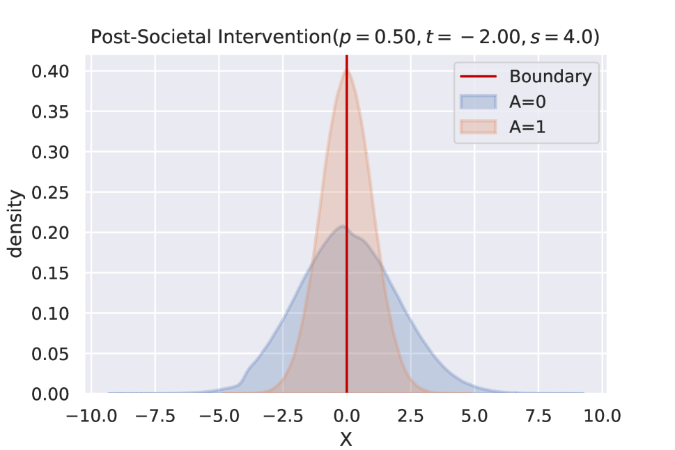
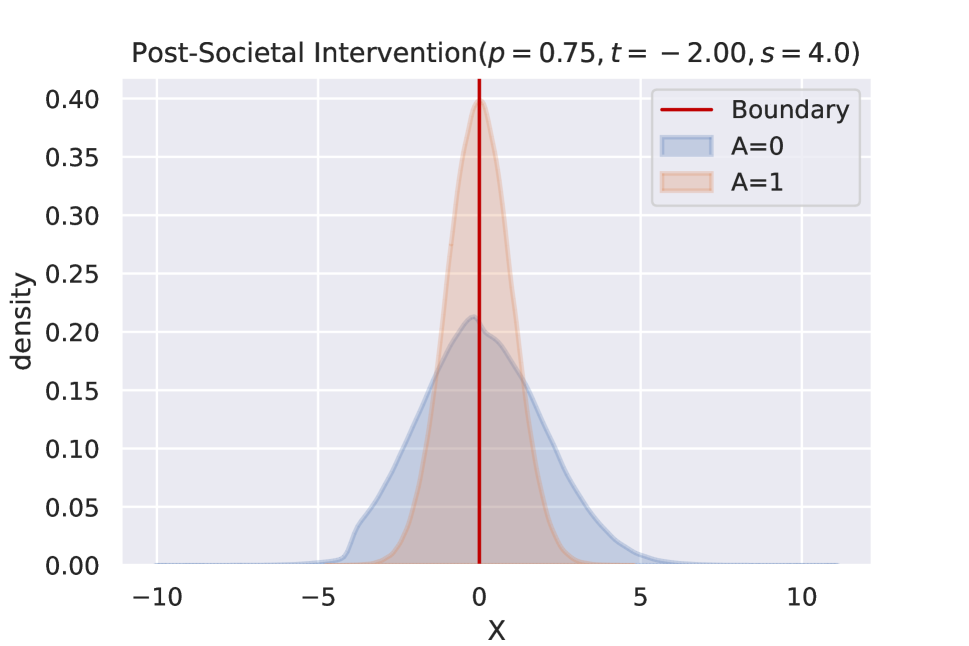
We demonstrate our ideas for the toy example with different variances across groups from Fig. 1. Here, the difference in recourse cost across groups cannot easily be resolved by changing the classifier $h$ (e.g., per the techniques in § 3.4): to achieve perfectly fair recourse, we would have to use a constant classifier, i.e., either approve all credit cards, or none, irrespective of income. Essentially, changing $h$ does not address the root of the problem, namely the discrepancy in the two populations. Instead, we investigate how to reduce the larger cost of recourse within the higher-variance group by altering the data generating process via societal interventions.

(a) Post-intervention distribution

(b) Comparison of different societal interventions

Figure 4: (a) Distribution after applying a societal intervention to the credit-card example from Fig. 1. We randomly select a proportion $p=1$ of individuals from the disadvantaged group (blue, $A=0$) to receive a subsidy $s=1.5$ if $U_{X}$ is below the threshold $t=-0.75$. As a result, the distribution of negatively-classified individuals ($X<0$) shifts towards the boundary which makes it more similar to those in $A=1$, thus resulting in fairer recourse. At the same time, the distribution of positively-classified individuals ($X>0$) remains unchanged. (b) Comparison of different societal interventions $i_{k}=(1,t,-2t)$ with respect to their benefit (reduction in recourse difference) and cost (paid-out subsidies). The threshold $t\approx-0.75$ (corresponding to the distribution shown on the left) leads to the largest reduction in recourse difference, but also incurs the highest cost. Smaller reductions can be achieved using two different thresholds: one corresponding to giving a larger subsidy to fewer individuals, and the other to giving a smaller subsidy to more individuals.

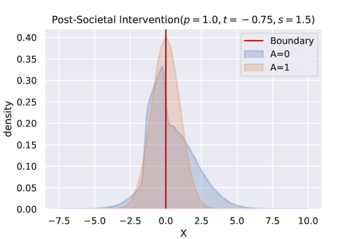
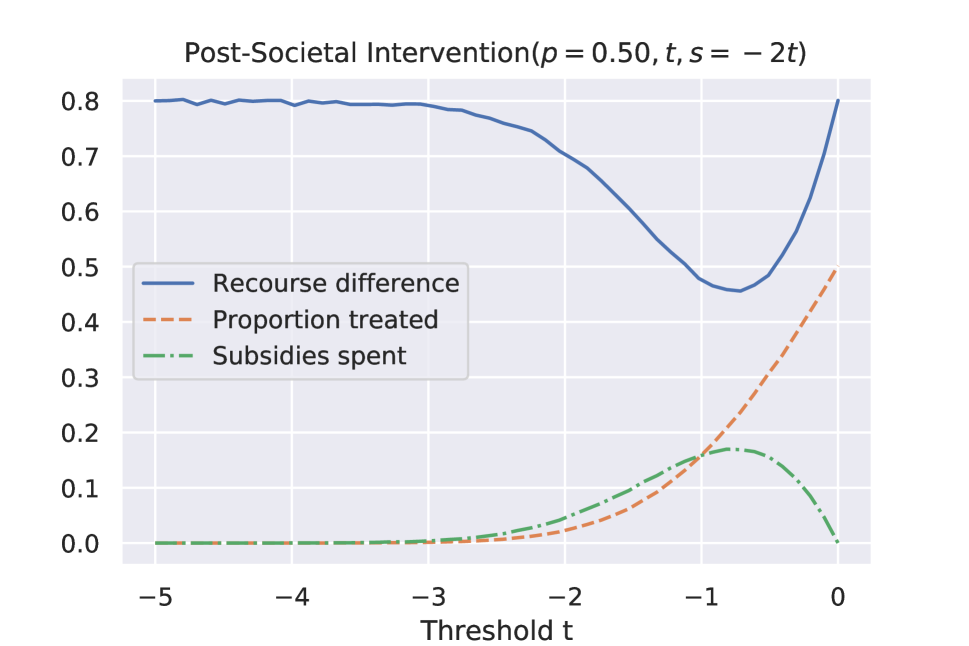
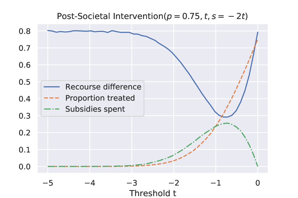
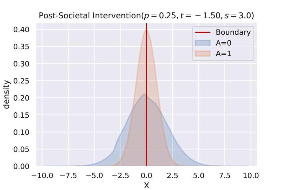
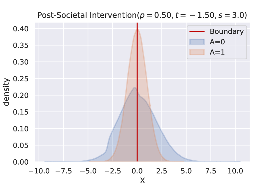
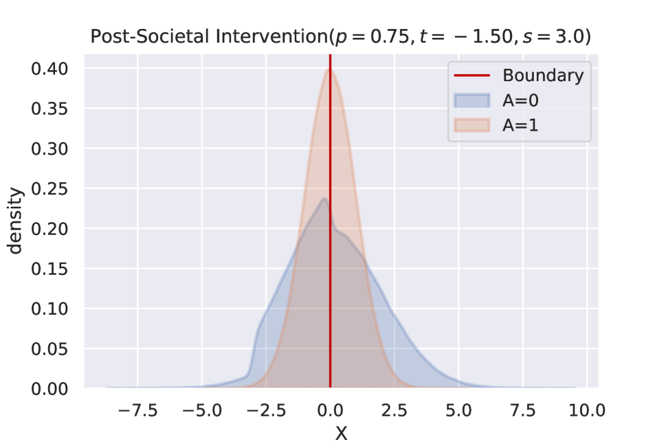
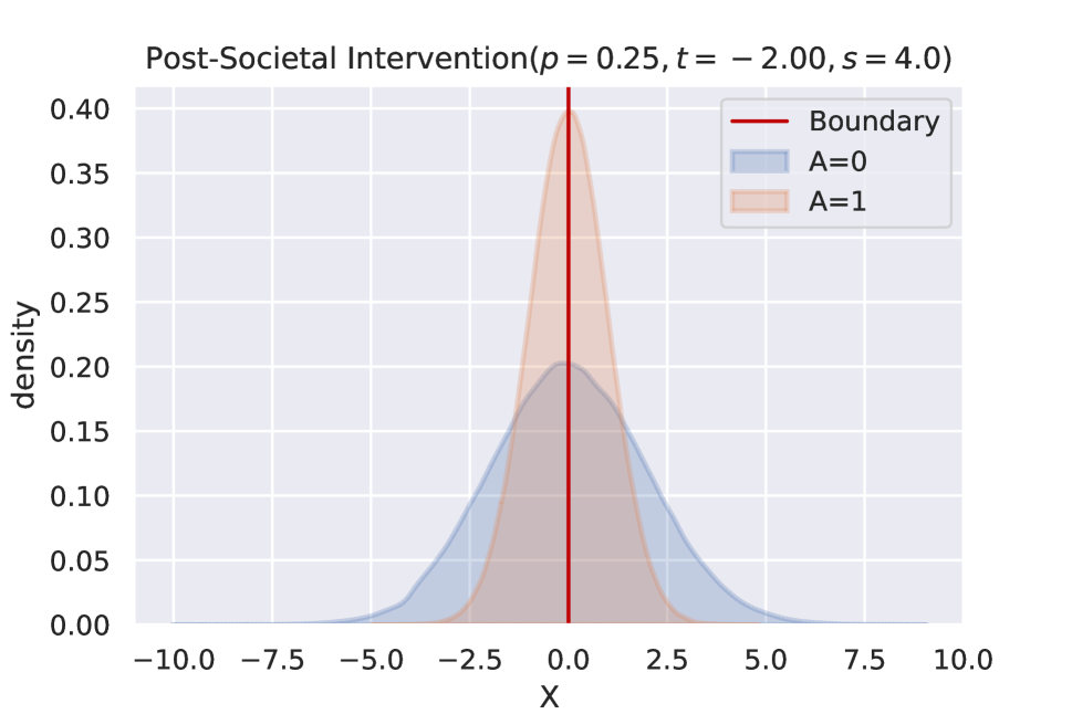
Let $i_{k}$ denote a societal intervention that modifies the data generating process, $X:=(2-A)U_{X}$, $U_{X}\sim\mathcal{N}(0,1)$, by changing the original SCM $\mathcal{M}$ to $\mathcal{M}^{\prime}_{k}=i_{k}(\mathcal{M})$. For example, $i_{k}$ may introduce additional variables or modify a subset of the original structural equations. Specifically, we consider subsidies to particular eligible individuals. We introduce a new treatment variable $T$ which randomly selects a proportion $0\leq p\leq 1$ of individuals from $A=0$ who are awarded a subsidy $s$ if their latent variable $U_{X}$ is below a threshold $t$. This is captured by the modified structural equations

$$\textstyle T :=(1-A)\mathbb{I}\{U_{T}<p\}, U_{T} \sim\text{Uniform}[0,1],$$

$$X :=(2-A)U_{X}+sT\mathbb{I}\{U_{X}<t\}, U_{X} \sim\mathcal{N}(0,1).$$

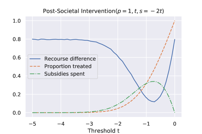
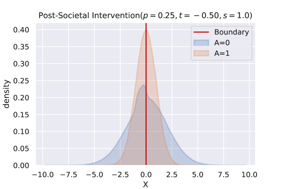
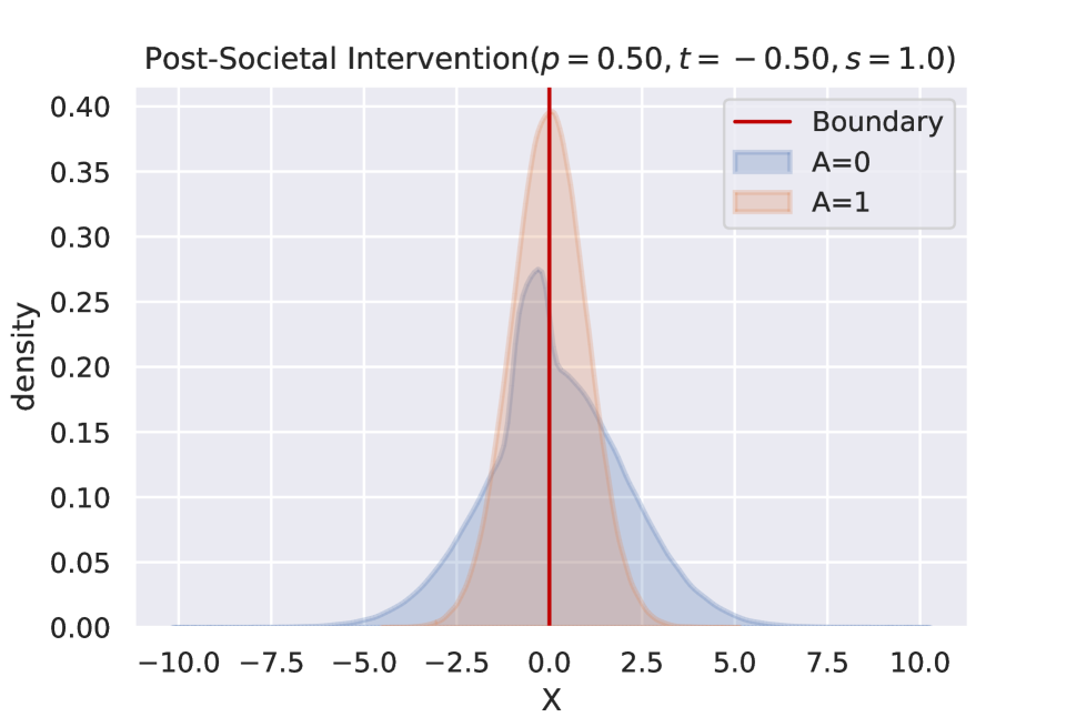
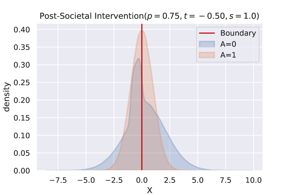
Here, each societal intervention $i_{k}$ thus corresponds to a particular way of setting the triple $(p,t,s)$. To avoid changing the predictions $\mathrm{sgn}(X)$, we only consider $t\leq 0$ and $s\leq-2t$. The modified distribution resulting from $i_{k}=(1,-0.75,1.5)$ is shown in Fig. 4(a), see the caption for details.

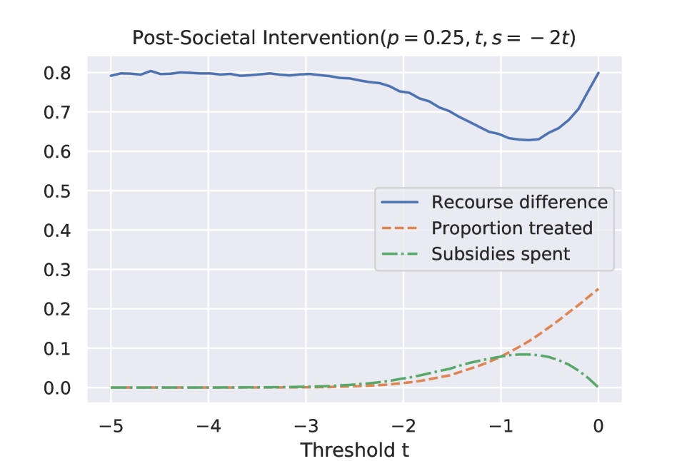
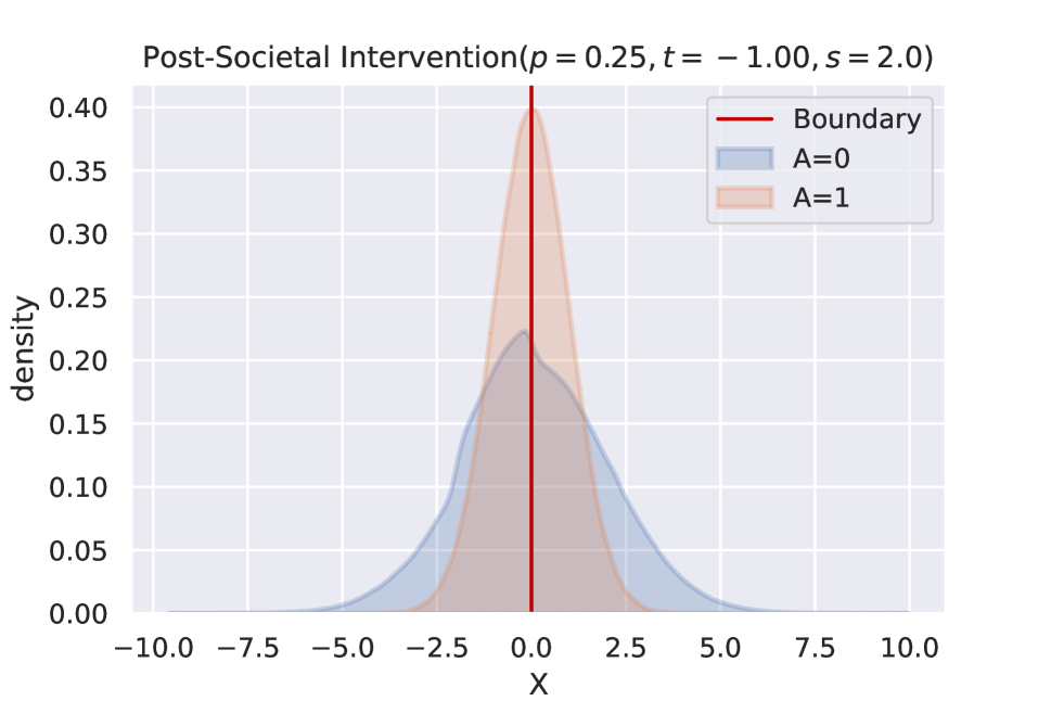
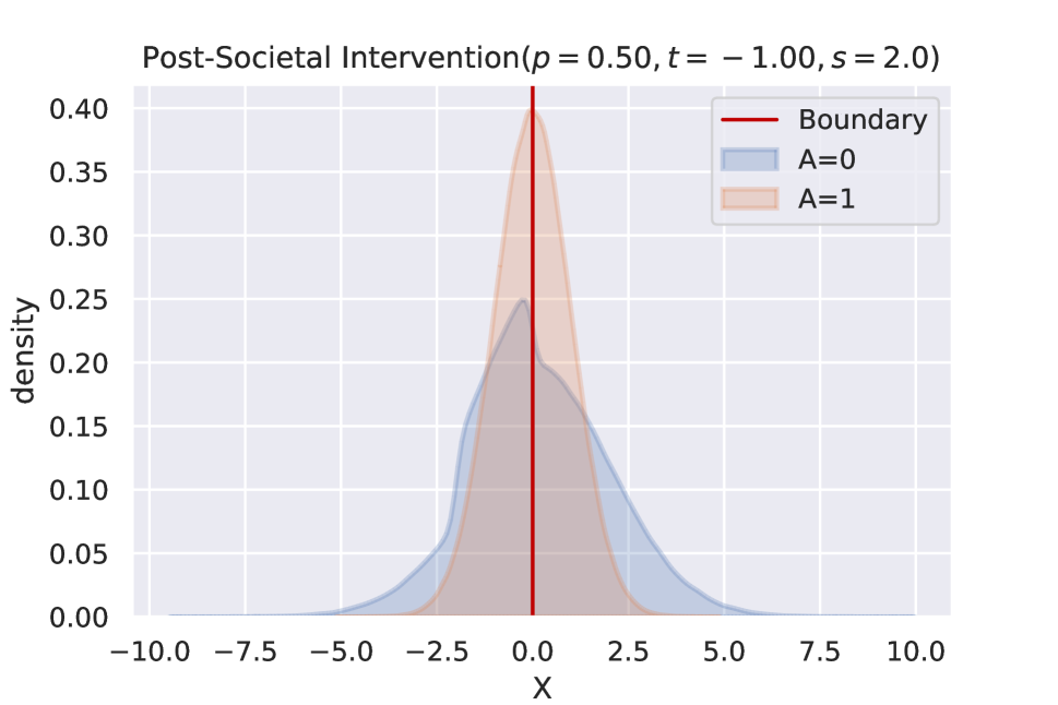
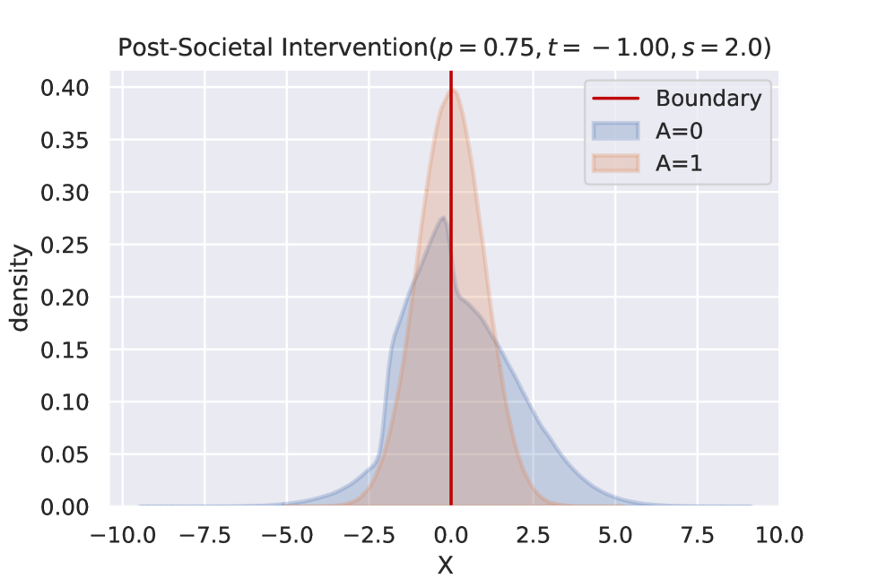
To evaluate the effectiveness of different societal interventions $i_{k}$ in reducing recourse unfairness, we compare their associated societal costs $c_{k}$ and benefits $b_{k}$. Here, the cost $c_{k}$ of implementing $i_{k}$ can reasonably be chosen as the total amount of paid-out subsidies, and the benefit $b_{k}$, as the reduction in the difference of average recourse cost across groups. We then reason about different societal interventions $i_{k}$ by simulating the proposed change via sampling data from $\mathcal{M}^{\prime}_{k}$ and computing $b_{k}$ and $c_{k}$ based on the simulated data. To decide which intervention to implement, we compare the societal benefit $b_{k}$ and cost $c_{k}$ of $i_{k}$ for different $k$ and choose the one with the most favourable trade-off. We show the societal benefit and cost tradeoff for $i_{k}=(1,t,-2t)$ with varying $t$ in Fig. 4(b) and refer to the caption for further details. Plots similar to Fig. 4 for different choices of $(p,t,s)$ are shown in Fig. 5 in § B.1. Effectively, our societal intervention does not change the outcome of credit card approval but ensures that the effort required (additional income needed) for rejected individuals from two groups is the same. Instead of using a threshold to select eligible individuals as in the toy example above, for more complex settings, our individual-level unfairness metric (Defn. 3.2) may provide a useful way to inform whom to target with societal interventions as it can be used to identify individuals for whom the counterfactual difference in recourse cost is particularly high.

6 Discussion

With data-driven decision systems pervading our societies, establishing appropriate fairness metrics and paths to recourse are gaining major significance. There is still much work to do in identifying and conceptually understanding the best path forward. Here we make progress towards this goal by applying tools of graphical causality. We are hopeful that this approach will continue to be fruitful as we search together with stakeholders and broader society for the right concepts and definitions, as well as for assaying interventions on societal mechanisms.

While our fairness criteria may help assess the fairness of recourse, it is still unclear how best to achieve fair causal recourse algorithmically. Here, we argue that fairness considerations may benefit from considering the larger system at play—instead of focusing solely on the classifier—and that a causal model of the underlying data generating process provides a principled framework for addressing issues such as multiple sources of unfairness, as well as different costs and benefits to individuals, institutions, and society.

Societal interventions to overcome (algorithmic) discrimination constitute a complex topic which not only applies to fair recourse but also to other notions of fairness. It deserves further study well beyond the scope of the present work. We may also question whether it is appropriate to perform a societal intervention on all individuals in a subgroup. For example, when considering who is approved for a credit card, an individual might not be able to pay their statements on time and this could imply costs to them, to the bank, or to society. This idea relates to the economics literature which studies the effect of policy interventions on society, institutions, and individuals (Heckman and Vytlacil 2005; Heckman 2010). Thus, future work could focus on formalising the effect of these interventions to the SCM, as such a framework would help trade off the costs and benefits for individuals, companies, and society.

Appendix A Experimental Details

In this Appendix, we provide additional details on our experiment setup.

A.1 SCM Specification

First, we give the exact form of SCMs used to generate our three synthetic data sets IMF, CAU-LIN, and CAU-ANM. Besides the desired characteristics of independently-manipulable (IMF) or causally dependent (CAU) features and linear (LIN) or nonlinear (ANM) relationships with additive noise, we choose the particular form of structural equations for each setting such that all features are roughly standardised, i.e., such that they all approximately have a mean of zero and a variance one.

We use the causal structures shown in Fig. 3. Apart from the desire two make the causal graphs similar to facilitate a better comparison and avoid introducing further nuisance factors while respecting the different structural constraints of the IMF and CAU settings, this particular choice is motivated by having at least one feature which is not a descendant of the protected attribute $A$. This is so that LR/SVM($\mathbf{X}_{\text{nd}(A)}$) and LR/SVM($\mathbf{X}_{\text{nd}(A)},\mathbf{U}_{\text{d}(A)}$) always have access to at least one actionable variable ($X_{2}$) which can be manipulated to achieve recourse.

IMF

For the IMF data sets, we sample the protected attribute $A$ and the features $X_{i}$ according to the following SCM:

$$A :=2U_{A}-1, U_{A}\sim\mathrm{Bernoulli}(0.5)$$

$$X_{1} :=0.5A+U_{1}, U_{1}\sim\mathcal{N}(0,1)$$

$$X_{2} :=U_{2}, U_{2}\sim\mathcal{N}(0,1)$$

$$X_{3} :=0.5A+U_{3}, U_{3}\sim\mathcal{N}(0,1)$$

CAU-LIN

For the CAU-LIN data sets, we sample $A$ and $X_{i}$ according to the following SCM:

$$A :=2U_{A}-1, U_{A}\sim\mathrm{Bernoulli}(0.5)$$

$$X_{1} :=0.5A+U_{1}, U_{1}\sim\mathcal{N}(0,1)$$

$$X_{2} :=U_{2}, U_{2}\sim\mathcal{N}(0,1)$$

$$X_{3} :=0.5(A+X_{1}-X_{2})+U_{3}, U_{3}\sim\mathcal{N}(0,1)$$

CAU-ANM

For the CAU-ANM data sets, we sample $A$ and $X_{i}$ according to the following SCM:

$$A :=2U_{A}-1, U_{A}\sim\mathrm{Bernoulli}(0.5)$$

$$X_{1} :=0.5A+U_{1}, U_{1}\sim\mathcal{N}(0,1)$$

$$X_{2} :=U_{2}, U_{2}\sim\mathcal{N}(0,1)$$

$$X_{3} :=0.5A+0.1(X_{1}^{3}-X_{2}^{3})+U_{3}, U_{3}\sim\mathcal{N}(0,1)$$

A.2 Label generation

To generate ground truth labels on which the different classifiers are trained, we consider both a linear and a nonlinear logistic regression. Specifically, we generate ground truth labels according to

$$Y:=\mathbb{I}\{U_{Y}<h(X_{1},X_{2},X_{3})\},\quad\quad U_{Y}\sim\mathrm{Uniform}[0,1].$$

In the linear case, $h(X_{1},X_{2},X_{3})$ is given by

$$h(X_{1},X_{2},X_{3})=\left(1+e^{-2(X_{1}-X_{2}+X_{3})}\right)^{-1}.$$

In the nonlinear case, $h(X_{1},X_{2},X_{3})$ is given by

$$h(X_{1},X_{2},X_{3})=\left(1+e^{4-(X_{1}+2X_{2}+X_{3})^{2}}\right)^{-1}.$$

A.3 Fair model architectures and training hyper-parameters

We use the implementation of Gupta et al. (2019) for the FairSVM and the sklearn SVC class (Pedregosa et al. 2011) for all other SVM variants. We consider the following values of hyperparameters (which are the same as those reported in (Gupta et al. 2019) for ease of comparison) and choose the best by 5-fold cross validation (unless stated otherwise): $\text{kernel type}\in\{\text{linear, poly, rbf}\}$, regularisation strength $C\in\{1,10,100\}$, RBF kernel bandwidth $\gamma_{\textsc{rbf}}\in\{0.001,0.01,0.1,1\}$, polynomial kernel $\text{degree}\in\{2,3,5\}$; following (Gupta et al. 2019), we also pick the fairness trade-off parameter $\lambda=\{0.2,0.5,1,2,10,50,100\}$ by cross-validation.

For the nonlinear logistic regression model, we opted for an instance of the sklearn MLPClassifier class with two hidden layers (10 neurons each) and ReLU activation functions. This model was then optimised on its inputs using the default optimiser and training hyperparameters.

A.4 Optimisation approach

Since an algorithmic contribution for solving the causal recourse optimisation problem is not the main focus of this work, we choose to discretise the space of possible recourse actions and select the best (i.e., lowest cost) valid action by performing a brute-force search. For an alternative gradient-based approach to solving the causal recourse optimisation problem, we refer to (Karimi et al. 2020c).

For each actionable feature $X_{i}$, denote by $\max_{i}$ and $\min_{i}$ its maximum and minimum attained in the training set, respectively. Given a factual observation $x^{\texttt{F}}_{i}$ of $X_{i}$, we discretise the search space and pick possible intervention values $\theta_{i}$ using 15 equally-spaced bins in the range $[x^{\texttt{F}}_{i}-2(x^{\texttt{F}}_{i}-\min_{i}),x^{\texttt{F}}_{i}+2(\max_{i}-x^{\texttt{F}}_{i})]$. We then consider all possible combinations of intervention values over all subsets $\mathcal{I}$ of the actionable variables. We note that for LR/SVM$(\mathbf{X}_{\text{nd}})$ and LR/SVM$(\mathbf{X}_{\text{nd}},\mathbf{U}_{\text{d}})$, only $X_{2}$ is actionable, while for the other LR/SVMs all of $\{X_{1},X_{2},X_{3}\}$ are actionable.

A.5 Adult dataset case study

The causal graph for the Adult dataset informed by expert knowledge (Nabi and Shpitser 2018; Chiappa 2019) is depicted in Fig. 3(c).

Because the true structural equations are not known, we learn an approximate SCM for the Adult dataset by fitting each parent-child relationship in the causal graph. Since most variables in the Adult dataset are categorical, additive noise is not an appropriate assumption for most of them. We therefore opt for modelling each structural equation, $X_{i}:=f_{i}(\text{PA}_{i},U_{i})$, using a latent variable model; specifically, we use a conditional variational autoencoder (CVAE) (Sohn, Lee, and Yan 2015), similar to (Karimi et al. 2020c).

We use deterministic conditional decoders $D_{i}(\text{PA}_{i},U_{i};\psi_{i})$, implemented as neural nets parametrised by $\psi_{i}$, and use an isotropic Gaussian prior, $U_{i}\sim\mathcal{N}(0,\mathbf{I})$, for each $X_{i}$.

For continuous features, the decoders directly output the value assigned to $X_{i}$, i.e., we approximate the structural equations as

$$X_{i}^{\text{continuous}}:=D_{i}(\text{PA}_{i},U_{i};\psi_{i}),\quad\quad U_{i}\sim\mathcal{N}(0,\mathbf{I}).$$ (8)

For categorical features, the decoders output a vector of class probabilities (by applying a softmax operation after the last layer). The arg max is then assigned as the value of the corresponding categorical feature, i.e.,

$$X_{i}^{\text{categorical}}:=\operatorname*{arg\,max}D_{i}(\text{PA}_{i},U_{i};\psi_{i}),\quad\quad U_{i}\sim\mathcal{N}(0,\mathbf{I}).$$ (9)

The decoders $D_{i}(\text{PA}_{i},U_{i};\psi_{i})$ are trained using the standard variational framework (Kingma and Welling 2014; Rezende, Mohamed, and Wierstra 2014), amortised with approximate Gaussian posteriors $q_{\phi_{i}}(U_{i}|X_{i},\text{PA}_{i})$ whose means and variances are computed by encoders in the form of neural nets with parameters $\phi_{i}$. For continuous features, we use the standard reconstruction error between real-valued predictions and targets, i.e., L$2$/MSE$(X_{i},D_{i}(\text{PA}_{i},U_{i};\psi_{i}))$, whereas for categorical features, we instead use the cross entropy loss between the one-hot encoded value of $X_{i}$ and the predicted vector of class probabilities, i.e., $\text{CrossEnt}(X_{i},\text{softmax}(D_{i}(\text{PA}_{i},U_{i};\psi_{i}))$.

The CVAEs are trained on $6,000$ training samples using a fixed learning rate of $0.05$, and a batch size of $128$ for $100$ epochs with early stopping on a held-out validation set of $250$ samples. For each parent-child relation, we train 10 models with the number of hidden layers and units randomly drawn from the following configurations for the encoder: $\text{enc}_{\text{arch}}=\{(\zeta,2,2),(\zeta,3,3),(\zeta,5,5),(\zeta,32,32,32)\}$, where $\zeta$ is the input dimensionality; and similarly for the decoders from: $\text{dec}_{\text{arch}}=\{(2,\eta),(2,2,\eta),(3,3,\eta),(5,5,\eta),(32,32,32,\eta)\}$, where $\eta$ is either one for continuous variables, or alternatively the size of the one-hot embedding for categorical variables (e.g., Work Class, Marital Status, and Occupation have 7, 10, and 14 categories, respectively). Moreover, we also randomly pick a latent dimension from $\{1,3,5\}$. We then select the model with the smallest MMD score (Gretton et al. 2012) between true instances and samples from the decoder post-training.

To perform abduction for counterfactual reasoning with such an approximate CVAE-SCM, we sample $U_{i}$ from the approximate posterior. For further discussion, we refer to (Karimi et al. 2020c), Appendix C.

Finally, using this approximate SCM, we solve the recourse optimisation problem similar to the synthetic experiments above. The caveat with this approach (and any real-world dataset absent a true SCM for that matter) is that we are not able to certify that a given recourse action generated under the assumption of an approximate SCM will guarantee recourse when executed in the true world governed by the real (unknown) SCM.

Appendix B Additional Results

In this Appendix, we provide additional experimental results omitted from the main paper due to space constraints.

B.1 Additional Societal Interventions

In § 5, we only showed plots for $i_{k}$ with $p=1$ since this has the largest potential to reduce recourse unfairness. However, it may not be feasible to give subsidies to all eligible individuals, and so, for completeness, we also show plots similar to Fig. 4 for different choices of $(p,t,s)$ in Fig. 5.

Figure 5: Plots for additional societal interventions $i_{k}=(p,t,s)$ in the context of the credit card approval example. We consider budgets of $p=0.25$ (left column), $p=0.5$ (middle column), and $p=0.75$ (right column). In the top row, we show the difference across groups in the average distance to the decision boundary for negatively classified individuals (recourse difference), the proportion of negatively-classified individuals in the disadvantaged group $A=0$ who received the treatment (proportion treated), and the amount of subsidies actually paid out to these individuals (subsidies spent) as a function of the threshold $t$. Note that the subsidy amount is fixed to its maximum amount without affecting the label distribution, i.e., $s=-2t$. In rows 2-5, we show the feature distribution resulting from $i_{k}=(p,t,s)$ with $t=-2s\in\{-0.5,-1,-1.5,-2\}$, see the plot titles for the exact values.

B.2 Using different SCMs for Recourse

The results presented in § 4.1 of the main paper use an estimate $\hat{\mathcal{M}}_{\textsc{kr}}$ of the ground truth SCM $\mathcal{M}^{\star}$ (learnt via kernel ridge regression under an additive noise assumption) to solve the recourse optimisation problem.

In Tab. 3 we show a more complete account of results which also includes the cases where the ground truth SCM $\mathcal{M}^{\star}$ or a linear ($\hat{\mathcal{M}}_{\textsc{LIN}}$) estimate thereof is used as the basis for computing recourse actions. When using an SCM estimate for recourse, we only consider valid actions to compute $\Delta_{\textbf{cost}}$ and $\Delta_{\textbf{ind}}$, where the validity of an action is determined by whether it results in a changed prediction according the oracle $\mathcal{M}^{\star}$.

We find that, as expected, using different SCMs does not affect Acc or $\Delta_{\textbf{dist}}$ since these metrics are, by definition, agnostic to the underlying causal generative process encoded by the SCM. However, using an estimated SCM in place of the true one may result in different values for $\Delta_{\textbf{cost}}$ and $\Delta_{\textbf{ind}}$ since these metrics take the downstream effects of recourse actions on other features into account and thus depend on the underlying SCM, c.f. Defns. 3.1 and 3.2.

We observe that using an estimated SCM may lead to underestimating or overestimating the true fair causal recourse metric (without any apparent clear trend as to when one or the other occurs). Moreover, the mis-estimation of fair causal recourse metrics is particularly pronounced when using the linear SCM estimate $\hat{\mathcal{M}}_{\textsc{LIN}}$ in a scenario in which the true SCM is, in fact, nonlinear, i.e., on the CAU-ANM data sets. This behaviour is intuitive and to be expected and should caution against using overly strong assumptions or too simplistic parametric models when estimating an SCM for use in (fair) recourse. We also remark that, in practice, underestimation of the true fairness metric is probably more problematic than overestimation.

Despite some small differences, the overall trends reported in § 4.1 remain very much the same, and thus seem relatively robust to small differences in the SCM which is used to compute recourse actions.

B.3 Kernel selection by cross validation

For completeness, we perform the same set of experiments shown in Tab. 3 where we also choose the kernel function by cross validation, instead of fixing it to either a linear or a polynomial kernel as before. The results are shown in Tab. 4 and the overall trends, again, remain largely the same.

As expected, we observe variations in accuracy compared to Tab. 3 due to the different kernel choice. Perhaps most interestingly, the FairSVM seems to generally perform slightly better in terms of $\Delta_{\textbf{dist}}$ when given the “free” choice of kernel, especially on the first three data sets with linearly generated labels. This suggests that the use of a nonlinear kernel may be important for FairSVM to achieve its goal.

However, we caution that the results in Tab. 4 may not be easily comparable across classifiers as distances are computed in the induced feature spaces which are either low-dimensional (in case of a linear kernel), high-dimensional (in case of a polynomial kernel), or infinite-dimensional (in case of an RBF kernel), which is also why we chose to report results based on the same kernel type in § 4.

Table 3: Complete account of experimental results corresponding to the setting described in § 4 of the main paper, where we additionally consider using the true SCM $\mathcal{M}^{\star}$ or a linear $(\hat{\mathcal{M}}_{\text{LIN}})$ estimate thereof to infer the latent variables $\mathbf{U}$ and solve the recourse optimisation problem. We compare different classifiers with respect to accuracy and different recourse fairness metrics on our three synthetic data sets with ground truth labels drawn from either a linear or a nonlinear logistic regression. For ease of comparison, we use the same kernel for all SVM variants for a given dataset: a linear kernel for linearly generated ground truth labels and a polynomial kernel for non-linearly generated ground truth labels. Moreover, linear (resp. nonlinear) logistic regression classifiers are used for linearly (resp. nonlinearly) generated ground truth labels. All other hyper-parameters are chosen by 10-fold cross-validation. We use a dataset of 500 observations for all experiments and make sure that it is roughly balanced, both with respect to the protected attribute $A$ and the label $Y$. Accuracies (higher is better) are computed on a separate i.i.d. test set of equal size. Fairness metrics (lower is better) are computed based on randomly selecting 50 negatively-classified samples from each of the two protected groups and using these to compute the difference between group-wise averages ($\Delta_{\textbf{dist}}$ and $\Delta_{\textbf{cost}}$) and maximum individual unfairness. When using an SCM estimate for recourse, we only consider valid actions to compute $\Delta_{\textbf{cost}}$ and $\Delta_{\textbf{ind}}$, where the validity of an action is determined by whether it results in a changed prediction according the oracle $\mathcal{M}^{\star}$. For each experiment and metric, the best performing method is highlighted in bold.

SCM	Classifier	GT labels from linear log. reg. $\rightarrow$ using linear kernel / linear log. reg.												GT labels from nonlinear log. reg. $\rightarrow$ using polynomial kernel / nonlinear log. reg.
		IMF				CAU-LIN				CAU-ANM				IMF				CAU-LIN				CAU-ANM
		Acc	$\Delta_{\textbf{dist}}$	$\Delta_{\textbf{cost}}$	$\Delta_{\textbf{ind}}$	Acc	$\Delta_{\textbf{dist}}$	$\Delta_{\textbf{cost}}$	$\Delta_{\textbf{ind}}$	Acc	$\Delta_{\textbf{dist}}$	$\Delta_{\textbf{cost}}$	$\Delta_{\textbf{ind}}$	Acc	$\Delta_{\textbf{dist}}$	$\Delta_{\textbf{cost}}$	$\Delta_{\textbf{ind}}$	Acc	$\Delta_{\textbf{dist}}$	$\Delta_{\textbf{cost}}$	$\Delta_{\textbf{ind}}$	Acc	$\Delta_{\textbf{dist}}$	$\Delta_{\textbf{cost}}$	$\Delta_{\textbf{ind}}$
$\mathcal{M}^{\star}$	SVM$(\mathbf{X},A)$	86.5	0.96	0.40	1.63	89.5	1.18	0.43	2.11	88.2	0.65	0.12	2.41	90.8	0.05	0.00	1.09	91.1	0.07	0.04	1.06	90.6	0.04	0.07	1.40
	LR$(\mathbf{X},A)$	86.7	0.48	0.50	1.91	89.5	0.63	0.49	2.11	87.7	0.40	0.22	2.41	90.5	0.08	0.03	1.06	90.6	0.09	0.02	1.00	90.6	0.19	0.18	1.28
	SVM$(\mathbf{X})$	86.4	0.99	0.42	1.80	89.4	1.61	0.61	2.11	88.0	0.56	0.12	2.79	91.4	0.13	0.00	0.92	91.0	0.17	0.09	1.09	91.0	0.02	0.02	1.64
	LR$(\mathbf{X})$	86.6	0.47	0.53	1.80	89.5	0.64	0.52	2.11	87.7	0.41	0.31	2.79	91.0	0.12	0.03	1.01	90.6	0.13	0.10	1.65	90.9	0.08	0.02	1.16
	FairSVM$(\mathbf{X},A)$	68.1	0.04	0.28	1.36	66.8	0.26	0.12	0.78	66.3	0.25	0.21	1.50	90.1	0.02	0.00	1.15	90.7	0.06	0.04	1.16	90.3	0.37	0.03	1.64
	SVM$(\mathbf{X}_{\text{nd}(A)})$	65.5	0.05	0.06	0.00	67.4	0.15	0.17	0.00	65.9	0.31	0.37	0.00	66.7	0.10	0.06	0.00	58.4	0.05	0.06	0.00	62.0	0.13	0.11	0.00
	LR$(\mathbf{X}_{\text{nd}(A)})$	65.3	0.05	0.05	0.00	67.3	0.18	0.18	0.00	65.6	0.31	0.31	0.00	64.7	0.02	0.04	0.00	58.4	0.02	0.02	0.00	61.1	0.02	0.03	0.00
	SVM$(\mathbf{X}_{\text{nd}(A)},\mathbf{U}_{\text{d}(A)})$	86.5	0.96	0.58	0.00	89.6	1.07	0.70	0.00	88.0	0.21	0.14	0.00	90.7	0.02	0.03	0.00	91.1	0.15	0.11	0.00	90.1	0.15	0.12	0.00
	LR$(\mathbf{X}_{\text{nd}(A)},\mathbf{U}_{\text{d}(A)})$	86.7	0.43	0.90	0.00	89.5	0.35	0.77	0.00	87.8	0.14	0.34	0.00	90.9	0.28	0.05	0.00	90.9	0.49	0.07	0.00	90.2	0.43	0.21	0.00
$\hat{\mathcal{M}}_{\text{LIN}}$	SVM$(\mathbf{X},A)$	86.5	0.96	0.40	1.63	89.5	1.18	0.44	2.11	88.2	0.65	0.30	3.77	90.8	0.05	0.00	1.09	91.1	0.07	0.04	1.06	90.6	0.04	0.04	1.49
	LR$(\mathbf{X},A)$	86.7	0.48	0.50	1.91	89.5	0.63	0.51	2.11	87.7	0.40	0.43	3.77	90.5	0.08	0.03	1.06	90.6	0.09	0.01	1.00	90.6	0.19	0.20	1.28
	SVM$(\mathbf{X})$	86.4	0.99	0.42	1.80	89.4	1.61	0.61	2.11	88.0	0.56	0.20	3.48	91.4	0.13	0.00	0.92	91.0	0.17	0.10	1.09	91.0	0.02	0.03	1.49
	LR$(\mathbf{X})$	86.6	0.47	0.53	1.80	89.5	0.64	0.58	2.11	87.7	0.41	0.55	3.48	91.0	0.12	0.03	1.01	90.6	0.13	0.10	1.65	90.9	0.08	0.04	1.66
	FairSVM$(\mathbf{X},A)$	68.1	0.04	0.28	1.36	66.8	0.26	0.12	0.78	66.3	0.25	0.21	1.50	90.1	0.02	0.00	1.15	90.7	0.06	0.05	1.16	90.3	0.37	0.01	1.64
	SVM$(\mathbf{X}_{\text{nd}(A)})$	65.5	0.05	0.06	0.00	67.4	0.15	0.17	0.00	65.9	0.31	0.37	0.00	66.7	0.10	0.06	0.00	58.4	0.05	0.06	0.00	62.0	0.13	0.11	0.00
	LR$(\mathbf{X}_{\text{nd}(A)})$	65.3	0.05	0.05	0.00	67.3	0.18	0.18	0.00	65.6	0.31	0.31	0.00	64.7	0.02	0.04	0.00	58.4	0.02	0.02	0.00	61.1	0.02	0.03	0.00
	SVM$(\mathbf{X}_{\text{nd}(A)},\mathbf{U}_{\text{d}(A)})$	86.5	0.96	0.58	0.00	89.6	1.07	0.70	0.00	88.0	0.21	0.14	0.00	90.7	0.02	0.03	0.00	91.1	0.15	0.11	0.00	90.1	0.15	0.12	0.00
	LR$(\mathbf{X}_{\text{nd}(A)},\mathbf{U}_{\text{d}(A)})$	86.7	0.43	0.90	0.00	89.5	0.35	0.77	0.00	87.8	0.14	0.34	0.00	90.9	0.28	0.05	0.00	90.9	0.49	0.07	0.00	90.2	0.43	0.21	0.00
$\hat{\mathcal{M}}_{\text{KR}}$	SVM$(\mathbf{X},A)$	86.5	0.96	0.40	1.63	89.5	1.18	0.44	2.11	88.2	0.65	0.27	2.32	90.8	0.05	0.00	1.09	91.1	0.07	0.03	1.06	90.6	0.04	0.03	1.40
	LR$(\mathbf{X},A)$	86.7	0.48	0.50	1.91	89.5	0.63	0.53	2.11	87.7	0.40	0.34	2.32	90.5	0.08	0.03	1.06	90.6	0.09	0.01	1.00	90.6	0.19	0.22	1.28
	SVM$(\mathbf{X})$	86.4	0.99	0.42	1.80	89.4	1.61	0.61	2.11	88.0	0.56	0.29	2.79	91.4	0.13	0.00	0.92	91.0	0.17	0.08	1.09	91.0	0.02	0.03	1.64
	LR$(\mathbf{X})$	86.6	0.47	0.53	1.80	89.5	0.64	0.57	2.11	87.7	0.41	0.43	2.79	91.0	0.12	0.03	1.01	90.6	0.13	0.10	1.65	90.9	0.08	0.06	1.66
	FairSVM$(\mathbf{X},A)$	68.1	0.04	0.28	1.36	66.8	0.26	0.12	0.78	66.3	0.25	0.21	1.50	90.1	0.02	0.00	1.15	90.7	0.06	0.04	1.16	90.3	0.37	0.02	1.64
	SVM$(\mathbf{X}_{\text{nd}(A)})$	65.5	0.05	0.06	0.00	67.4	0.15	0.17	0.00	65.9	0.31	0.37	0.00	66.7	0.10	0.06	0.00	58.4	0.05	0.06	0.00	62.0	0.13	0.11	0.00
	LR$(\mathbf{X}_{\text{nd}(A)})$	65.3	0.05	0.05	0.00	67.3	0.18	0.18	0.00	65.6	0.31	0.31	0.00	64.7	0.02	0.04	0.00	58.4	0.02	0.02	0.00	61.1	0.02	0.03	0.00
	SVM$(\mathbf{X}_{\text{nd}(A)},\mathbf{U}_{\text{d}(A)})$	86.5	0.96	0.58	0.00	89.6	1.07	0.70	0.00	88.0	0.21	0.14	0.00	90.7	0.02	0.03	0.00	91.1	0.15	0.11	0.00	90.1	0.15	0.12	0.00
	LR$(\mathbf{X}_{\text{nd}(A)},\mathbf{U}_{\text{d}(A)})$	86.7	0.43	0.90	0.00	89.5	0.35	0.77	0.00	87.8	0.14	0.34	0.00	90.9	0.28	0.05	0.00	90.9	0.49	0.07	0.00	90.2	0.43	0.21	0.00

Table 4: Additional results where also the kernel (linear, polynomial, or rbf) for each SVM is chosen by 5-fold cross-validation instead of being fixed based on the ground truth label distribution. We remark that some metrics (e.g., $\Delta_{\textbf{dist}}$) may not be comparable across methods since they are computed in a different reference space when different kernels are selected. Otherwise the experimental setup is identical to that from Tab. 3, see the caption for details.

SCM	Classifier	GT labels from linear log. reg. $\rightarrow$ using cross-validated kernel / linear log. reg.												GT labels from nonlinear log. reg. $\rightarrow$ using cross-validated kernel / nonlinear log. reg.
		IMF				CAU-LIN				CAU-ANM				IMF				CAU-LIN				CAU-ANM
		Acc	$\Delta_{\textbf{dist}}$	$\Delta_{\textbf{cost}}$	$\Delta_{\textbf{ind}}$	Acc	$\Delta_{\textbf{dist}}$	$\Delta_{\textbf{cost}}$	$\Delta_{\textbf{ind}}$	Acc	$\Delta_{\textbf{dist}}$	$\Delta_{\textbf{cost}}$	$\Delta_{\textbf{ind}}$	Acc	$\Delta_{\textbf{dist}}$	$\Delta_{\textbf{cost}}$	$\Delta_{\textbf{ind}}$	Acc	$\Delta_{\textbf{dist}}$	$\Delta_{\textbf{cost}}$	$\Delta_{\textbf{ind}}$	Acc	$\Delta_{\textbf{dist}}$	$\Delta_{\textbf{cost}}$	$\Delta_{\textbf{ind}}$
$\mathcal{M}^{\star}$	SVM$(\mathbf{X},A)$	86.5	0.96	0.40	1.63	89.2	1.33	0.55	2.10	87.8	0.36	0.08	2.79	90.8	0.05	0.00	1.09	91.1	0.07	0.04	1.06	90.6	0.04	0.07	1.40
	LR$(\mathbf{X},A)$	86.7	0.48	0.50	1.91	89.5	0.63	0.49	2.11	87.7	0.40	0.22	2.41	90.5	0.08	0.03	1.06	90.6	0.09	0.02	1.00	90.6	0.19	0.18	1.28
	SVM$(\mathbf{X})$	86.4	0.99	0.42	1.80	89.5	1.13	0.53	2.14	87.6	0.43	0.42	2.79	91.4	0.13	0.00	0.92	91.0	0.17	0.09	1.09	89.4	0.16	0.16	1.16
	LR$(\mathbf{X})$	86.6	0.47	0.53	1.80	89.5	0.64	0.52	2.11	87.7	0.41	0.31	2.79	91.0	0.12	0.03	1.01	90.6	0.13	0.10	1.65	90.9	0.08	0.02	1.16
	FairSVM$(\mathbf{X},A)$	86.4	0.01	0.20	1.61	60.5	0.00	0.33	1.05	57.6	0.01	0.13	1.76	90.1	0.02	0.00	1.15	90.7	0.06	0.04	1.16	78.0	0.00	0.04	1.73
	SVM$(\mathbf{X}_{\text{nd}(A)})$	64.6	0.06	0.09	0.00	67.3	0.17	0.25	0.00	65.9	0.28	0.31	0.00	65.7	0.01	0.02	0.00	55.6	0.04	0.03	0.00	61.6	0.04	0.03	0.00
	LR$(\mathbf{X}_{\text{nd}(A)})$	65.3	0.05	0.05	0.00	67.3	0.18	0.18	0.00	65.6	0.31	0.31	0.00	64.7	0.02	0.04	0.00	58.4	0.02	0.02	0.00	61.1	0.02	0.03	0.00
	SVM$(\mathbf{X}_{\text{nd}(A)},\mathbf{U}_{\text{d}(A)})$	86.6	0.84	0.64	0.00	89.4	0.81	0.54	0.00	87.4	0.21	0.35	0.00	90.7	0.02	0.03	0.00	91.1	0.15	0.11	0.00	89.0	0.31	0.13	0.00
	LR$(\mathbf{X}_{\text{nd}(A)},\mathbf{U}_{\text{d}(A)})$	86.7	0.43	0.90	0.00	89.5	0.35	0.77	0.00	87.8	0.14	0.34	0.00	90.9	0.28	0.05	0.00	90.9	0.49	0.07	0.00	90.2	0.43	0.21	0.00
$\hat{\mathcal{M}}_{\text{LIN}}$	SVM$(\mathbf{X},A)$	86.5	0.96	0.40	1.63	89.2	1.33	0.55	2.10	87.8	0.36	0.13	3.48	90.8	0.05	0.00	1.09	91.1	0.07	0.04	1.06	90.6	0.04	0.04	1.49
	LR$(\mathbf{X},A)$	86.7	0.48	0.50	1.91	89.5	0.63	0.51	2.11	87.7	0.40	0.43	3.77	90.5	0.08	0.03	1.06	90.6	0.09	0.01	1.00	90.6	0.19	0.20	1.28
	SVM$(\mathbf{X})$	86.4	0.99	0.42	1.80	89.5	1.13	0.51	2.14	87.6	0.43	0.42	4.05	91.4	0.13	0.00	0.92	91.0	0.17	0.10	1.09	89.4	0.16	0.11	1.16
	LR$(\mathbf{X})$	86.6	0.47	0.53	1.80	89.5	0.64	0.58	2.11	87.7	0.41	0.55	3.48	91.0	0.12	0.03	1.01	90.6	0.13	0.10	1.65	90.9	0.08	0.04	1.66
	FairSVM$(\mathbf{X},A)$	86.4	0.01	0.20	1.61	60.5	0.00	0.29	1.05	57.6	0.01	0.12	1.76	90.1	0.02	0.00	1.15	90.7	0.06	0.05	1.16	78.0	0.00	0.03	1.73
	SVM$(\mathbf{X}_{\text{nd}(A)})$	64.6	0.06	0.09	0.00	67.3	0.17	0.25	0.00	65.9	0.28	0.31	0.00	65.7	0.01	0.02	0.00	55.6	0.04	0.03	0.00	61.6	0.04	0.03	0.00
	LR$(\mathbf{X}_{\text{nd}(A)})$	65.3	0.05	0.05	0.00	67.3	0.18	0.18	0.00	65.6	0.31	0.31	0.00	64.7	0.02	0.04	0.00	58.4	0.02	0.02	0.00	61.1	0.02	0.03	0.00
	SVM$(\mathbf{X}_{\text{nd}(A)},\mathbf{U}_{\text{d}(A)})$	86.6	0.84	0.64	0.00	89.4	0.81	0.54	0.00	87.4	0.21	0.35	0.00	90.7	0.02	0.03	0.00	91.1	0.15	0.11	0.00	89.0	0.31	0.13	0.00
	LR$(\mathbf{X}_{\text{nd}(A)},\mathbf{U}_{\text{d}(A)})$	86.7	0.43	0.90	0.00	89.5	0.35	0.77	0.00	87.8	0.14	0.34	0.00	90.9	0.28	0.05	0.00	90.9	0.49	0.07	0.00	90.2	0.43	0.21	0.00
$\hat{\mathcal{M}}_{\text{KR}}$	SVM$(\mathbf{X},A)$	86.5	0.96	0.40	1.63	89.2	1.33	0.56	2.10	87.8	0.36	0.18	2.79	90.8	0.05	0.00	1.09	91.1	0.07	0.03	1.06	90.6	0.04	0.03	1.40
	LR$(\mathbf{X},A)$	86.7	0.48	0.50	1.91	89.5	0.63	0.53	2.11	87.7	0.40	0.34	2.32	90.5	0.08	0.03	1.06	90.6	0.09	0.01	1.00	90.6	0.19	0.22	1.28
	SVM$(\mathbf{X})$	86.4	0.99	0.42	1.80	89.5	1.13	0.52	2.14	87.6	0.43	0.44	2.79	91.4	0.13	0.00	0.92	91.0	0.17	0.08	1.09	89.4	0.16	0.14	1.16
	LR$(\mathbf{X})$	86.6	0.47	0.53	1.80	89.5	0.64	0.57	2.11	87.7	0.41	0.43	2.79	91.0	0.12	0.03	1.01	90.6	0.13	0.10	1.65	90.9	0.08	0.06	1.66
	FairSVM$(\mathbf{X},A)$	86.4	0.01	0.20	1.61	60.5	0.00	0.26	1.50	57.6	0.01	0.12	1.76	90.1	0.02	0.00	1.15	90.7	0.06	0.04	1.16	78.0	0.00	0.01	1.73
	SVM$(\mathbf{X}_{\text{nd}(A)})$	64.6	0.06	0.09	0.00	67.3	0.17	0.25	0.00	65.9	0.28	0.31	0.00	65.7	0.01	0.02	0.00	55.6	0.04	0.03	0.00	61.6	0.04	0.03	0.00
	LR$(\mathbf{X}_{\text{nd}(A)})$	65.3	0.05	0.05	0.00	67.3	0.18	0.18	0.00	65.6	0.31	0.31	0.00	64.7	0.02	0.04	0.00	58.4	0.02	0.02	0.00	61.1	0.02	0.03	0.00
	SVM$(\mathbf{X}_{\text{nd}(A)},\mathbf{U}_{\text{d}(A)})$	86.6	0.84	0.64	0.00	89.4	0.81	0.54	0.00	87.4	0.21	0.35	0.00	90.7	0.02	0.03	0.00	91.1	0.15	0.11	0.00	89.0	0.31	0.13	0.00
	LR$(\mathbf{X}_{\text{nd}(A)},\mathbf{U}_{\text{d}(A)})$	86.7	0.43	0.90	0.00	89.5	0.35	0.77	0.00	87.8	0.14	0.34	0.00	90.9	0.28	0.05	0.00	90.9	0.49	0.07	0.00	90.2	0.43	0.21	0.00

References

- Arneson (2015) Arneson, R. 2015. Equality of Opportunity. In Zalta, E. N., ed., The Stanford Encyclopedia of Philosophy. Metaphysics Research Lab, Stanford University, Summer 2015 edition.
- Barocas, Selbst, and Raghavan (2020) Barocas, S.; Selbst, A. D.; and Raghavan, M. 2020. The hidden assumptions behind counterfactual explanations and principal reasons. In Proceedings of the 2020 Conference on Fairness, Accountability, and Transparency, 80–89.
- Chiappa (2019) Chiappa, S. 2019. Path-specific counterfactual fairness. In Proceedings of the AAAI Conference on Artificial Intelligence, volume 33, 7801–7808.
- Chouldechova (2017) Chouldechova, A. 2017. Fair prediction with disparate impact: A study of bias in recidivism prediction instruments. Big data, 5(2): 153–163.
- Dwork et al. (2012) Dwork, C.; Hardt, M.; Pitassi, T.; Reingold, O.; and Zemel, R. 2012. Fairness through awareness. In Proceedings of the 3rd innovations in theoretical computer science conference, 214–226.
- Gretton et al. (2012) Gretton, A.; Borgwardt, K. M.; Rasch, M. J.; Schölkopf, B.; and Smola, A. 2012. A kernel two-sample test. The Journal of Machine Learning Research, 13(1): 723–773.
- Grgić-Hlača et al. (2017) Grgić-Hlača, N.; Zafar, M. B.; Gummadi, K.; and Weller, A. 2017. On Fairness, Diversity, and Randomness in Algorithmic Decision Making. In 4th Workshop on Fairness, Accountability, and Transparency in Machine Learning.
- Gupta et al. (2019) Gupta, V.; Nokhiz, P.; Roy, C. D.; and Venkatasubramanian, S. 2019. Equalizing Recourse across Groups. arXiv preprint arXiv:1909.03166.
- Hardt, Price, and Srebro (2016) Hardt, M.; Price, E.; and Srebro, N. 2016. Equality of opportunity in supervised learning. In Advances in neural information processing systems, 3315–3323.
- Heckman (2010) Heckman, J. J. 2010. Building bridges between structural and program evaluation approaches to evaluating policy. Journal of Economic literature, 48(2): 356–98.
- Heckman and Vytlacil (2005) Heckman, J. J.; and Vytlacil, E. 2005. Structural equations, treatment effects, and econometric policy evaluation 1. Econometrica, 73(3): 669–738.
- Joshi et al. (2019) Joshi, S.; Koyejo, O.; Vijitbenjaronk, W.; Kim, B.; and Ghosh, J. 2019. Towards realistic individual recourse and actionable explanations in black-box decision making systems. arXiv preprint arXiv:1907.09615.
- Karimi et al. (2020a) Karimi, A.-H.; Barthe, G.; Balle, B.; and Valera, I. 2020a. Model-agnostic counterfactual explanations for consequential decisions. In International Conference on Artificial Intelligence and Statistics, 895–905.
- Karimi et al. (2020b) Karimi, A.-H.; Barthe, G.; Schölkopf, B.; and Valera, I. 2020b. A survey of algorithmic recourse: definitions, formulations, solutions, and prospects. arXiv preprint arXiv:2010.04050.
- Karimi, Schölkopf, and Valera (2021) Karimi, A.-H.; Schölkopf, B.; and Valera, I. 2021. Algorithmic recourse: from counterfactual explanations to interventions. In Proceedings of the 2021 ACM Conference on Fairness, Accountability, and Transparency, 353–362.
- Karimi et al. (2020c) Karimi, A.-H.; von Kügelgen, J.; Schölkopf, B.; and Valera, I. 2020c. Algorithmic recourse under imperfect causal knowledge: a probabilistic approach. In Advances in Neural Information Processing Systems, volume 33, 265–277.
- Kilbertus et al. (2017) Kilbertus, N.; Carulla, M. R.; Parascandolo, G.; Hardt, M.; Janzing, D.; and Schölkopf, B. 2017. Avoiding discrimination through causal reasoning. In Advances in Neural Information Processing Systems, 656–666.
- Kingma and Welling (2014) Kingma, D. P.; and Welling, M. 2014. Auto-Encoding Variational Bayes. In 2nd International Conference on Learning Representations.
- Kusner et al. (2017) Kusner, M. J.; Loftus, J.; Russell, C.; and Silva, R. 2017. Counterfactual fairness. In Advances in Neural Information Processing Systems, 4066–4076.
- Lichman et al. (2013) Lichman, M.; et al. 2013. UCI machine learning repository. https://archive.ics.uci.edu/ml/datasets/adult.
- Loftus et al. (2018) Loftus, J. R.; Russell, C.; Kusner, M. J.; and Silva, R. 2018. Causal reasoning for algorithmic fairness. arXiv preprint arXiv:1805.05859.
- Mahajan, Tan, and Sharma (2019) Mahajan, D.; Tan, C.; and Sharma, A. 2019. Preserving Causal Constraints in Counterfactual Explanations for Machine Learning Classifiers. arXiv preprint arXiv:1912.03277.
- Mothilal, Sharma, and Tan (2020) Mothilal, R. K.; Sharma, A.; and Tan, C. 2020. Explaining machine learning classifiers through diverse counterfactual explanations. In Proceedings of the 2020 Conference on Fairness, Accountability, and Transparency, 607–617.
- Nabi, Malinsky, and Shpitser (2019) Nabi, R.; Malinsky, D.; and Shpitser, I. 2019. Learning optimal fair policies. In International Conference on Machine Learning, 4674–4682. PMLR.
- Nabi and Shpitser (2018) Nabi, R.; and Shpitser, I. 2018. Fair inference on outcomes. In Proceedings of the AAAI Conference on Artificial Intelligence.
- Pearl (2009) Pearl, J. 2009. Causality. Cambridge University Press.
- Pedregosa et al. (2011) Pedregosa, F.; Varoquaux, G.; Gramfort, A.; Michel, V.; Thirion, B.; Grisel, O.; Blondel, M.; Prettenhofer, P.; Weiss, R.; Dubourg, V.; et al. 2011. Scikit-learn: Machine learning in Python. Journal of Machine Learning Research, 12: 2825–2830.
- Peters, Janzing, and Schölkopf (2017) Peters, J.; Janzing, D.; and Schölkopf, B. 2017. Elements of causal inference. MIT Press.
- Rezende, Mohamed, and Wierstra (2014) Rezende, D. J.; Mohamed, S.; and Wierstra, D. 2014. Stochastic backpropagation and approximate inference in deep generative models. In International Conference on Machine Learning, 1278–1286. PMLR.
- Russell et al. (2017) Russell, C.; Kusner, M. J.; Loftus, J.; and Silva, R. 2017. When worlds collide: integrating different counterfactual assumptions in fairness. In Advances in Neural Information Processing Systems, 6414–6423.
- Salimi et al. (2019) Salimi, B.; Rodriguez, L.; Howe, B.; and Suciu, D. 2019. Interventional fairness: Causal database repair for algorithmic fairness. In Proceedings of the 2019 International Conference on Management of Data, 793–810.
- Schölkopf and Smola (2002) Schölkopf, B.; and Smola, A. J. 2002. Learning with Kernels. Cambridge, MA, USA: MIT Press.
- Sharma, Henderson, and Ghosh (2019) Sharma, S.; Henderson, J.; and Ghosh, J. 2019. CERTIFAI: Counterfactual Explanations for Robustness, Transparency, Interpretability, and Fairness of Artificial Intelligence models. arXiv preprint arXiv:1905.07857.
- Sohn, Lee, and Yan (2015) Sohn, K.; Lee, H.; and Yan, X. 2015. Learning structured output representation using deep conditional generative models. Advances in Neural Information Processing Systems, 28: 3483–3491.
- Upadhyay, Joshi, and Lakkaraju (2021) Upadhyay, S.; Joshi, S.; and Lakkaraju, H. 2021. Towards Robust and Reliable Algorithmic Recourse. In Thirty-Fifth Conference on Neural Information Processing Systems.
- Ustun, Spangher, and Liu (2019) Ustun, B.; Spangher, A.; and Liu, Y. 2019. Actionable recourse in linear classification. In Proceedings of the Conference on Fairness, Accountability, and Transparency, 10–19.
- Venkatasubramanian and Alfano (2020) Venkatasubramanian, S.; and Alfano, M. 2020. The philosophical basis of algorithmic recourse. In Proceedings of the 2020 Conference on Fairness, Accountability, and Transparency, 284–293.
- Wachter, Mittelstadt, and Russell (2017) Wachter, S.; Mittelstadt, B.; and Russell, C. 2017. Counterfactual explanations without opening the black box: Automated decisions and the GDPR. Harvard Journal of Law & Technology, 31(2).
- Wu, Zhang, and Wu (2019) Wu, Y.; Zhang, L.; and Wu, X. 2019. Counterfactual fairness: Unidentification, bound and algorithm. In Proceedings of the Twenty-Eighth International Joint Conference on Artificial Intelligence.
- Wu et al. (2019) Wu, Y.; Zhang, L.; Wu, X.; and Tong, H. 2019. Pc-fairness: A unified framework for measuring causality-based fairness. In Advances in Neural Information Processing Systems, 3404–3414.
- Zafar et al. (2017a) Zafar, M. B.; Valera, I.; Gomez Rodriguez, M.; and Gummadi, K. P. 2017a. Fairness beyond disparate treatment & disparate impact: Learning classification without disparate mistreatment. In Proceedings of the 26th International Conference on World Wide Web, 1171–1180.
- Zafar et al. (2017b) Zafar, M. B.; Valera, I.; Rogriguez, M. G.; and Gummadi, K. P. 2017b. Fairness constraints: Mechanisms for fair classification. In Artificial Intelligence and Statistics, 962–970. PMLR.
- Zemel et al. (2013) Zemel, R.; Wu, Y.; Swersky, K.; Pitassi, T.; and Dwork, C. 2013. Learning fair representations. In International Conference on Machine Learning, 325–333.
- Zhang and Bareinboim (2018a) Zhang, J.; and Bareinboim, E. 2018a. Equality of opportunity in classification: A causal approach. In Advances in Neural Information Processing Systems, 3671–3681.
- Zhang and Bareinboim (2018b) Zhang, J.; and Bareinboim, E. 2018b. Fairness in decision-making—the causal explanation formula. In Proceedings of the AAAI Conference on Artificial Intelligence.