Graph Information Bottleneck for Subgraph Recognition
Abstract
Given the input graph and its label/property, several key problems of graph learning, such as finding interpretable subgraphs, graph denoising and graph compression, can be attributed to the fundamental problem of recognizing a subgraph of the original one. This subgraph shall be as informative as possible, yet contains less redundant and noisy structure. This problem setting is closely related to the well-known information bottleneck (IB) principle, which, however, has less been studied for the irregular graph data and graph neural networks (GNNs). In this paper, we propose a framework of Graph Information Bottleneck (GIB) for the subgraph recognition problem in deep graph learning. Under this framework, one can recognize the maximally informative yet compressive subgraph, named IB-subgraph. However, the GIB objective is notoriously hard to optimize, mostly due to the intractability of the mutual information of irregular graph data and the unstable optimization process. In order to tackle these challenges, we propose: i) a GIB objective based-on a mutual information estimator for the irregular graph data; ii) a bi-level optimization scheme to maximize the GIB objective; iii) a connectivity loss to stabilize the optimization process. We evaluate the properties of the IB-subgraph in three application scenarios: improvement of graph classification, graph interpretation and graph denoising. Extensive experiments demonstrate that the information-theoretic IB-subgraph enjoys superior graph properties.
1 Introduction
Classifying the underlying labels or properties of graphs is a fundamental problem in deep graph learning with applications across many fields, such as biochemistry and social network analysis. However, real world graphs are likely to contain redundant even noisy information [9, 36], which poses a huge negative impact for graph classification. This triggers an interesting problem of recognizing an informative yet compressed subgraph from the original graph. For example, in drug discovery, when viewing molecules as graphs with atoms as nodes and chemical bonds as edges, biochemists are interested in identifying the subgraphs that mostly represent certain properties of the molecules, namely the functional groups [17, 11]. In graph representation learning, the predictive subgraph highlights the vital substructure for graph classification, and provides an alternative way for yielding graph representation besides mean/sum aggregation [19, 30, 32] and pooling aggregation [35, 21, 4]. In graph attack and defense, it is vital to purify a perturbed graph and mine the robust structures for classification [16].
Recently, the mechanism of self-attentive aggregation [22] somehow discovers a vital substructure at node level with a well-selected threshold. However, this method only identifies isolated important nodes but ignores the topological information at subgraph level. Consequently, it leads to a novel challenge as subgraph recognition: How can we recognize a compressed subgraph with minimum information loss in terms of predicting the graph labels/properties?
Recalling the above challenge, there is a similar problem setting in information theory called information bottleneck (IB) principle [29], which aims to juice out a compressed data from the original data that keeps most predictive information of labels or properties. Enhanced with deep learning, IB can learn informative representation from regular data in the fields of computer vision [24, 1, 23], reinforcement learning [13, 15] and natural language precessing [31]. However, current IB methods, like VIB [1], is still incapable for irregular graph data. It is still challenging for IB to compress irregular graph data, like a subgraph from an original graph, with a minimum information loss.
Hence, we advance the IB principle for irregular graph data to resolve the proposed subgraph recognition problem, which leads to a novel principle, Graph Information Bottleneck (GIB). Different from prior researches in IB that aims to learn an optimal representation of the input data in the hidden space, GIB directly reveals the vital substructure in the subgraph level. We first i) leverage the mutual information estimator from Deep Variational Information Bottleneck (VIB) [1] for irregular graph data as the GIB objective. However, VIB is intractable to compute the mutual information without knowing the distribution forms, especially on graph data. To tackle this issue, ii) we adopt a bi-level optimization scheme to maximize the GIB objective. Meanwhile, the continuous relaxation that we adopt to approach the discrete selection of subgraph will lead to unstable optimization process. To further stabilize the training process and encourage a compact subgraph, iii) we propose a novel connectivity loss to assist GIB to effectively discover the maximally informative but compressed subgraph, which is defined as IB-subgraph. By optimizing the above GIB objective and connectivity loss, one can recognize the IB-subgraph without any explicit subgraph annotation. On the other hand, iv) GIB is model-agnostic and can be easily plugged into various Graph Neural Networks (GNNs).
We evaluate the properties of the IB-subgraph in three application scenarios: improvement of graph classification, graph interpretation, and graph denoising. Extensive experiments on both synthetic and real world datasets demonstrate that the information-theoretic IB-subgraph enjoys superior graph properties compared to the subgraphs found by SOTA baselines.
2 Related Work
Graph Classification. In recent literature, there is a surge of interest in adopting graph neural networks (GNN) in graph classification. The core idea is to aggregate all the node information for graph representation. A typical implementation is the mean/sum aggregation [19, 32], which is to average or sum up the node embeddings. An alternative way is to leverage the hierarchical structure of graphs, which leads to the pooling aggregation [35, 38, 21, 4]. When tackling with the redundant and noisy graphs, these approaches will likely to result in sub-optimal graph representation.
Information Bottleneck. Information bottleneck (IB), originally proposed for signal processing, attempts to find a short code of the input signal but preserve maximum information of the code [29]. [1] firstly bridges the gap between IB and the deep learning, and proposed variational information bottleneck (VIB). Nowadays, IB and VIB have been wildly employed in computer vision [24, 23], reinforcement learning [13, 15], natural language processing [31] and speech and acoustics [25] due to the capability of learning compact and meaningful representations. However, IB is less researched on irregular graphs due to the intractability of mutual information.
Subgraph Discovery. Traditional subgraph discovery includes dense subgraph discovery and frequent subgraph mining. Dense subgraph discovery aims to find the subgraph with the highest density (e.g. the number of edges over the number of nodes [8, 12]). Frequent subgraph mining is to look for the most common substructure among graphs [33, 18, 37]. Recently, researchers discover the vital substructure at node level via the attention mechanism [30, 21, 20]. [34] further identifies the important computational graph for node classification. [2] discovers subgraph representations with specific topology given subgraph-level annotation.
3 Notations and Preliminaries
Let be a set of graphs with their real value properties or categories, where refers to the -th graph and refers to the corresponding properties or labels. We denote by the -th graph of size with node set , edge set , adjacent matrix , and feature matrix of with dimensions, respectively. Denote the neighborhood of as . We use as a specific subgraph and as the complementary structure of in . Let be the mapping from graphs to the real value property or category, , is the domain of the input graphs. refers to the Shannon mutual information of two random variables.
3.1 Graph convolutional network
Graph convolutional network (GCN) is widely adopted to graph classification. Given a graph with node feature and adjacent matrix , GCN outputs the node embeddings from the following process:
| (1) |
where refers to the diagonal matrix with nodes’ degrees and refers to the model parameters.
One can simply sum up the node embeddings to get a fixed length graph embeddings [32]. Recently, researchers attempt to exploit hierarchical structure of graphs, which leads to various graph pooling methods [22, 10, 21, 6, 38, 26, 35]. [22] enhances the graph pooling with self-attention mechanism to leverage the importance of different nodes contributing to the results. Finally, the graph embedding is obtained by multiplying the node embeddings with the normalized attention scores:
| (2) |
where and refers to the model parameters of self-attention.
3.2 Optimizing Information bottleneck objective
Given the input signal and the label , the objective of IB is maximized to find the the internal code : , where refers to a hyper-parameter trading off informativeness and compression. Optimizing this objective will lead to a compact but informative . [1] optimize a tractable lower bound of the IB objective:
| (3) |
where is the variational approximation to and is the prior distribution of . However, it is hard to estimate the mutual information in high dimensional space when the distribution forms are inaccessible, especially for irregular graph data.
4 Optimizing the Graph Information Bottleneck Objective for Subgraph Recognition
In this section, we will elaborate the proposed method in details. We first formally define the graph information bottleneck and IB-subgraph. Then, we introduce a novel framework for GIB to effectively find the IB-subgraph. We further propose a bi-level optimization scheme and a graph mutual information estimator for GIB optimization. Moreover, we do a continuous relaxation to the generation of subgraph, and propose a novel loss to stabilize the training process.
4.1 graph information bottleneck
We generalize the information bottleneck principle to learn a informative representation of irregular graphs, which leads to the graph information bottleneck (GIB) principle.
Definition 4.1 (Graph Information Bottleneck).
Given a graph and its label , the GIB seeks for the most informative yet compressed representation by optimizing the following objective:
| (4) |
where is the information constraint between and . By introducing a Lagrange multiplier to Eq. 4, we reach its unconstrained form:
| (5) |
Eq. 5 gives a general formulation of GIB. Here, in subgraph recognition, we focus on a subgraph which is compressed with minimum information loss in terms of graph properties.
Definition 4.2 (IB-subgraph).
For a graph , its maximally informative yet compressed subgraph, namely IB-subgraph can be obtained by optimizing the following objective:
| (6) |
where indicates the set of all subgraphs of .
IB-subgraph enjoys various pleasant properties and can be applied to multiple graph learning tasks such as improvement of graph classification, graph interpretation, and graph denoising. However, the GIB objective in Eq. 6 is notoriously hard to optimize due to the intractability of mutual information and the discrete nature of irregular graph data. We then introduce approaches on how to optimize such objective and derive the IB-subgraph.
4.2 Bi-level optimization for the GIB objective
The GIB objective in Eq. 6 consists of two parts. We examine the first term in Eq. 6, first. This term measures the relevance between and . We expand as:
| (7) |
is the entropy of and thus can be ignored. In practice, we approximate with an empirical distribution , where is the output subgraph and is the graph label. By substituting the true posterior with a variational approximation , we obtain a tractable lower bound of the first term in Eq. 6:
| (8) | ||||
where is the ground truth label of the graph. Eq. 8 indicates that maximizing is achieved by the minimization of the classification loss between and as . Intuitively, minimizing encourages the subgraph to be predictive of the graph label. In practice, we choose the cross entropy loss for categorical and the mean squared loss for continuous , respectively. For more details of deriving Eq. 7 and Eq. 8, please refer to Appendix A.1.
Then, we consider the minimization of which is the second term of Eq. 6. Remind that [1] introduces a tractable prior distribution in Eq. 3, and thus results in a variational upper bound. However, this setting is troublesome as it is hard to find a reasonable prior distribution for , which is the distribution of graph substructures instead of latent representation. Thus we go for another route. Directly applying the DONSKER-VARADHAN representation [7] of the KL-divergence, we have:
| (9) |
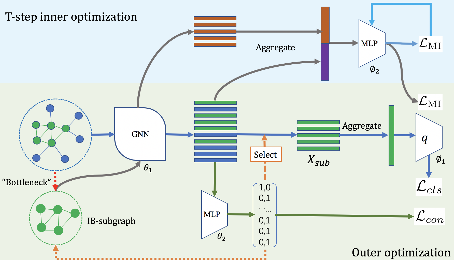
where is the statistics network that maps from the graph set to the set of real numbers. In order to approximate using Eq. 9, we design a statistics network based on modern GNN architectures as shown by Figure 1: first we use a GNN to extract embeddings from both and (parameter shared with the subgraph generator, which will be elaborated in Section 4.3), then concatenate and embeddings and feed them into a MLP, which finally produces the real number. In conjunction with the sampling method to approximate , and , we reach the following optimization problem to approximate111Notice that the MINE estimator [3] straightforwardly uses the DONSKER-VARADHAN representation to derive an MI estimator between the regular input data and its vectorized representation/encoding. It cannot be applied to estimate the mutual information between and since both of and are irregular graph data. :
| (10) |
With the approximation to the MI in graph data, we combine Eq. 6 , Eq. 8 and Eq. 10 and formulate the optimization process of GIB as a tractable bi-level optimization problem:
| (11) | |||
| (12) |
We first derive a sub-optimal notated as by optimizing Eq. 12 for T steps as inner loops. After the T-step optimization of the inner-loop ends, Eq. 10 is a proxy for MI minimization for the GIB objective as an outer loop. Then, the parameter and the subgraph are optimized to yield IB-subgraph. However, in the outer loop, the discrete nature of and hinders applying the gradient-based method to optimize the bi-level objective and find the IB-subgraph.
4.3 The Subgraph Generator and connectivity loss
To alleviate the discreteness in Eq. 11, we propose the continuous relaxation to the subgraph recognition and propose a loss to stabilize the training process.
Subgraph generator: For the input graph , we generate its IB-subgraph with the node assignment which indicates the node is in or . Then, we introduce a continuous relaxation to the node assignment with the probability of nodes belonging to the or . For example, the -th row of is 2-dimensional vector . We first use an -layer GNN to obtain the node embedding and employ a multi-layer perceptron (MLP) to output :
| (13) |
is a matrix, where is the number of nodes. For simplicity, we compile the above modules as the subgraph generator, denoted as with . When is well-learned, the assignment of nodes is supposed to saturate to 0/1. The representation of , which is employed for predicting the graph label, can be obtained by taking the first row of .
Connectivity loss: However, poor initialization will cause and to be close. This will either lead the model to assign all nodes to / , or result that the representations of contain much information from the redundant nodes. These two scenarios will cause the training process to be unstable. On the other hand, we suppose our model to have an inductive bias to better leverage the topological information while outputs the subgraph at a node-level. Therefore, we propose the following connectivity loss:
| (14) |
where is the row-wise normalization, is the Frobenius norm, and is a identity matrix. not only leads to distinguishable node assignment, but also encourage the subgraph to be compact. Take for example, denote the element 1,1 and the element 1,2 of ,
| (15) | |||
Minimizing results in . This occurs if is in , the elements of have a high probability in . Minimizing also encourages . This encourages and less cuts between and . This also holds for when analyzing and .
In a word, encourages distinctive to stabilize the training process and a compact topology in the subgraph. Therefore, the overall loss is:
| (16) | ||||
We provide the pseudo code in the Appendix to better illustrate how to optimize the above objective.
| Method | MUTAG | PROTEINS | IMDB-BINARY | DD |
|---|---|---|---|---|
| SortPool | 0.844 0.141 | 0.747 0.044 | 0.712 0.047 | 0.732 0.087 |
| ASAPool | 0.743 0.077 | 0.721 0.043 | 0.715 0.044 | 0.717 0.037 |
| DiffPool | 0.839 0.097 | 0.727 0.046 | 0.709 0.053 | 0.778 0.030 |
| EdgePool | 0.759 0.077 | 0.723 0.044 | 0.728 0.044 | 0.736 0.040 |
| AttPool | 0.721 0.086 | 0.728 0.041 | 0.722 0.047 | 0.711 0.055 |
| GCN | 0.7430.110 | 0.7190.041 | 0.707 0.037 | 0.725 0.046 |
| GraphSAGE | 0.7430.077 | 0.721 0.042 | 0.709 0.041 | 0.729 0.041 |
| GIN | 0.8250.068 | 0.707 0.056 | 0.732 0.048 | 0.730 0.033 |
| GAT | 0.738 0.074 | 0.714 0.040 | 0.713 0.042 | 0.695 0.045 |
| GCN+GIB | 0.776 0.075 | 0.748 0.046 | 0.722 0.039 | 0.765 0.050 |
| GraphSAGE+GIB | 0.760 0.074 | 0.734 0.043 | 0.719 0.052 | 0.781 0.042 |
| GIN+GIB | 0.839 0.064 | 0.749 0.051 | 0.737 0.070 | 0.747 0.039 |
| GAT+GIB | 0.749 0.097 | 0.737 0.044 | 0.729 0.046 | 0.769 0.040 |
| Method | QED | DRD2 | HLM-CLint | MLM-CLint |
| GCN+Att05 | 0.48 0.07 | 0.20 0.13 | 0.90 0.89 | 0.92 0.61 |
| GCN+Att07 | 0.41 0.07 | 0.16 0.11 | 1.18 0.60 | 1.69 0.88 |
| GCN+GIB w/o | 0.46 0.07 | 0.15 0.12 | 0.45 0.37 | 1.58 0.86 |
| GCN+GIB w/o | 0.43 0.15 | 0.21 0.13 | 0.48 0.34 | 1.20 0.97 |
| GCN+GIB | 0.38 0.12 | 0.06 0.09 | 0.37 0.30 | 0.72 0.55 |
5 Experiments
In this section, we evaluate the proposed GIB method on three scenarios, including improvement of graph classification, graph interpretation and graph denoising.
5.1 Baselines and settings
Improvement of graph classification: For improvement of graph classification, GIB generates graph representation by aggregating the subgraph information. We plug GIB into various backbones including GCN [19], GAT [30], GIN [32] and GraphSAGE [14]. We compare the proposed method with the mean/sum aggregation [19, 30, 14, 32] and pooling aggregation [38, 26, 35, 6] in terms of classification accuracy.
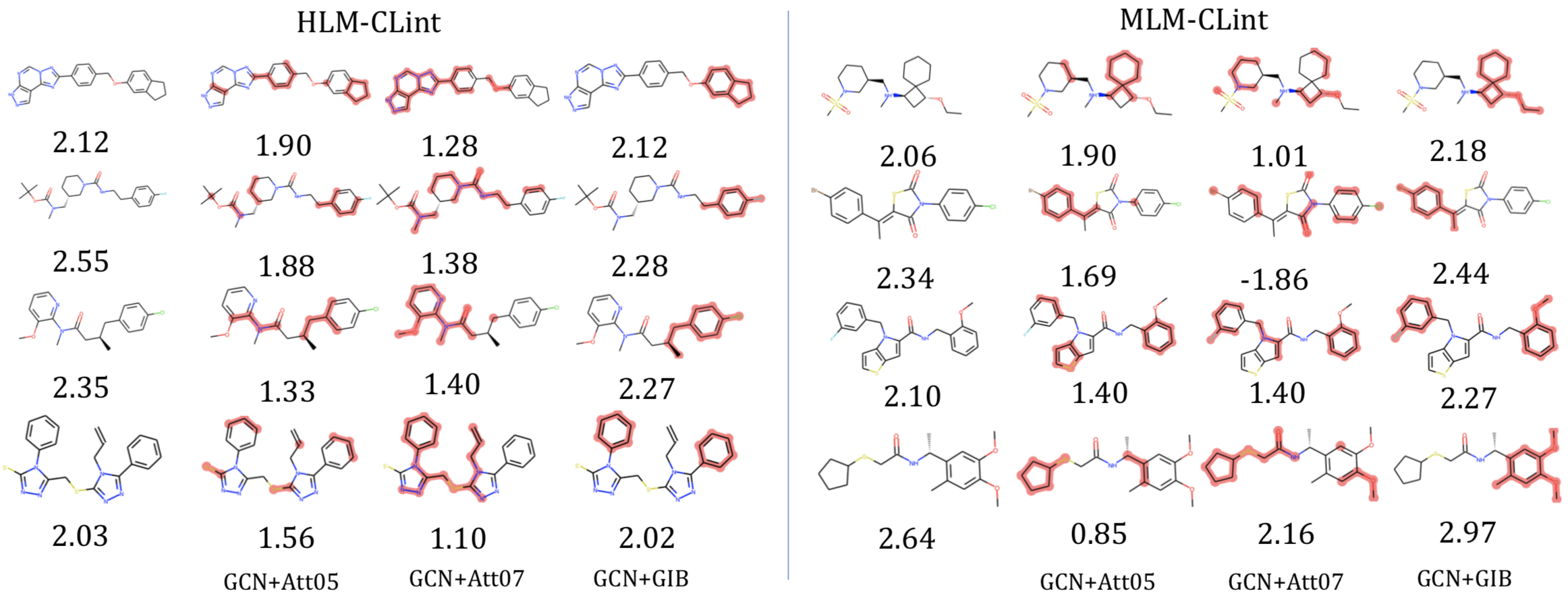
Graph interpretation: The goal of graph interpretation is to find the substructure which shares the most similar property to the molecule. If the substructure is disconnected, we evaluate its largest connected part. We compare GIB with the attention mechanism [22]. That is, we attentively aggregate the node information for graph prediction. The interpretable subgraph is generated by choosing the nodes with top and attention scores, namely Att05 and Att07. GIB outputs the interpretation with the IB-subgraph. Then, we evaluate the absolute property bias (the absolute value of the difference between the property of graph and subgraph) between the graph and its interpretation. For fare comparisons, we adopt the same GCN as the backbone for different methods.
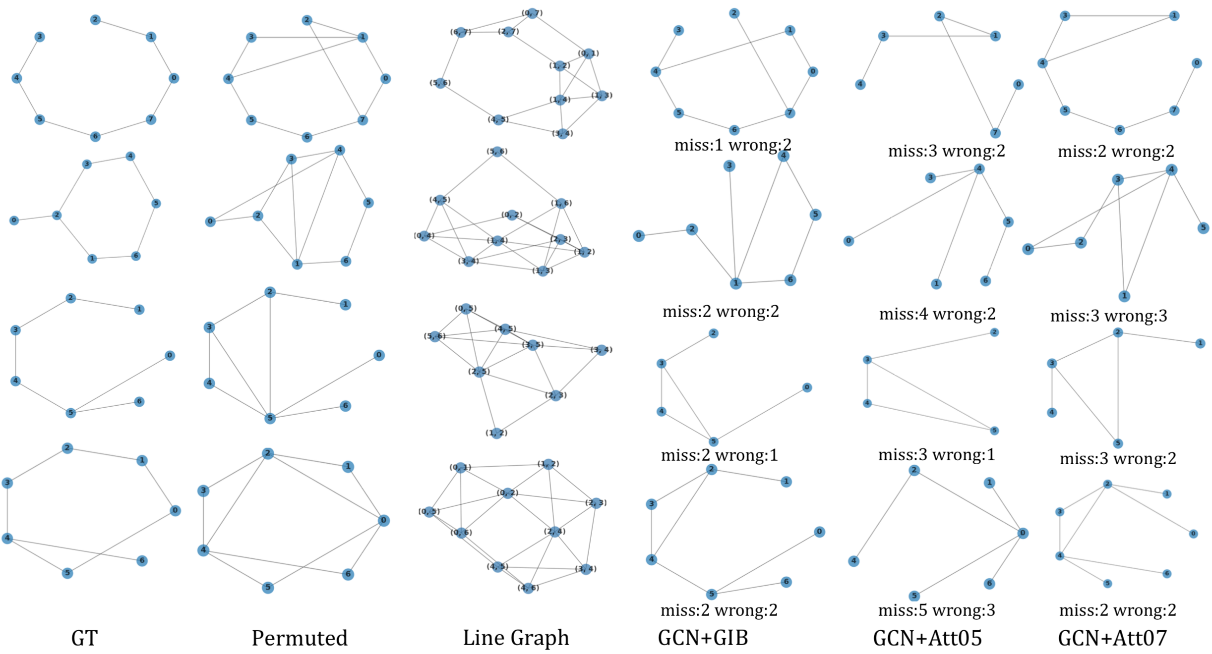
Graph denoising: We translate the permuted graph into the line-graph and use GIB and attention to 1) infer the real structure of graph, 2) classify the permuted graph via the inferred structure. We further compare the performance of GCN and DiffPool on the permuted graphs.
5.2 datasets
Improvement of graph classification: We evaluate different methods on the datasets of MUTAG [28], PROETINS [5], IMDB-BINARY and DD [27] datasets. 222We follow the protocol in https://github.com/rusty1s/pytorch_geometric/tree/master/benchmark/kernel.
Graph interpretation: We construct the datasets for graph interpretation on four molecule properties based on ZINC dataset, which contains 250K molecules. QED measures the drug likeness of a molecule, which is bounded within the range . DRD2 measures the probability that a molecule is active against dopamine type 2 receptor, which is bounded with . HLM-CLint and MLM-CLint are estimate values of in vitro human and mouse liver microsome metabolic stability (base 10 logrithm of mL/min/g). We sample the molecules with QED , DRD2 , HLM-CLint , MLM-CLint for each task. We use of these molecules for training, for validating and for testing.
Graph denoising: We generate a synthetic dataset by adding redundant edges for each graph in MUTAG dataset. We use of these graphs for training, for validating and for testing.
| Method | GCN | DiffPool | GCN+Att05 | GCN+Att07 | GCN+GIB |
|---|---|---|---|---|---|
| Recall | - | - | 0.2260.047 | 0.324 0.049 | 0.493 0.035 |
| Precision | - | - | 0.638 0.141 | 0.675 0.104 | 0.692 0.061 |
| Acc | 0.617 | 0.658 | 0.649 | 0.667 | 0.684 |
5.3 Results
Improvement of Graph Classification: In Table 1, we comprehensively evaluate the proposed method and baselines on improvement of graph classification. We train GIB on various backbones and aggregate the graph representations only from the subgraphs. We compare the performance of our framework with the mean/sum aggregation and pooling aggregation. This shows that GIB improves the graph classification by reducing the redundancies in the graph structure.
| Method | QED | DRD2 | HLM | MLM |
|---|---|---|---|---|
| GCN+Att05 | 3.38 | 1.94 | 3.11 | 5.16 |
| GCN+Att07 | 2.04 | 1.76 | 2.75 | 3.00 |
| GCN+GIB | 1.57 | 1.08 | 2.29 | 2.06 |
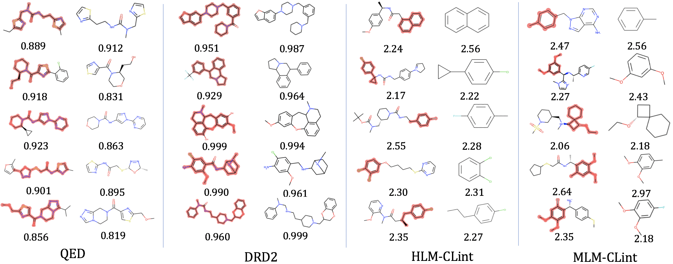
Graph interpretation: Table 2 shows the quantitative performance of different methods on the graph interpretation task. GIB is able to generate precise graph interpretation (IB-subgraph), as the substructures found by GIB has the most similar property to the input molecules. Then we derive two variants of our method by deleting and . GIB also outperforms the variants, and thus indicates that every part of our model does contribute to the improvement of performance. In practice, we observe that removing will lead to unstable training process due to the continuous relaxation to the generation of subgraph. In Fig. 2, GIB generates more compact and reasonable interpretation to the property of molecules confirmed by chemical experts. More results are provided in the Appendix. In Table 4, we compare the average number of disconnected substructures per graph since a compact subgraph should preserve more topological information. GIB generates more compact subgraphs to better interpret the graph property.
Graph denoising: Table 3 shows the performance of different methods on noisy graph classification. GIB outperforms the baselines on classification accuracy by a large margin due to the superior property of IB-subgraph. Moreover, GIB is able to better reveal the real structure of permuted graphs in terms of precision and recall rate of true edges.
6 Conclusion
In this paper, we have studied a subgraph recognition problem to infer a maximally informative yet compressed subgraph. We define such a subgraph as IB-subgraph and propose the graph information bottleneck (GIB) framework for effectively discovering an IB-subgraph. We derive the GIB objective from a mutual information estimator for irregular graph data, which is optimized by a bi-level learning scheme. A connectivity loss is further used to stabilize the learning process. We evaluate our GIB framework in the improvement of graph classification, graph interpretation and graph denoising. Experimental results verify the superior properties of IB-subgraphs.
References
- [1] Alexander A. Alemi, Ian Fischer, Joshua V. Dillon, and Kevin Murphy. Deep variational information bottleneck. In The International Conference on Representation Learning, 2017.
- [2] Emily Alsentzer, Samuel G. Finlayson, Michelle M. Li, and Marinka Zitnik. Subgraph neural networks. 2020.
- [3] Mohamed Ishmael Belghazi, Aristide Baratin, Sai Rajeswar, Sherjil Ozair, Yoshua Bengio, R. Devon Hjelm, and Aaron C. Courville. Mutual information neural estimation. In International Conference on Machine Learning, volume 80 of Proceedings of Machine Learning Research, pages 530–539, 2018.
- [4] Filippo Maria Bianchi, Daniele Grattarola, and Cesare Alippi. Spectral clustering with graph neural networks for graph pooling. In Proceedings of the 37th International Conference on Machine Learning, 2020.
- [5] Karsten M. Borgwardt, Cheng Soon Ong, Stefan Schanauer, S. V. N. Vishwanathan, Alexander J. Smola, and Hans-Peter Kriegel. Protein function prediction via graph kernels. In ISMB (Supplement of Bioinformatics), pages 47–56, 2005.
- [6] Frederik Diehl. Edge contraction pooling for graph neural networks. CoRR, abs/1905.10990, 2019.
- [7] M. D. Donsker and S. R. S. Varadhan. Asymptotic evaluation of certain markov process expectations for large time. Communications on Pure and Applied Mathematics, 36(2):183–212, 1983.
- [8] Yixiang Fang, Kaiqiang Yu, Reynold Cheng, Laks V. S. Lakshmanan, and Xuemin Lin. Efficient algorithms for densest subgraph discovery. Proceedings of VLDB Endowment, 12(11):1719–1732, 2019.
- [9] Luca Franceschi, Mathias Niepert, Massimiliano Pontil, and Xiao He. Learning discrete structures for graph neural networks. In ICML, volume 97 of Proceedings of Machine Learning Research, pages 1972–1982. PMLR, 2019.
- [10] Hongyang Gao and Shuiwang Ji. Graph u-nets. In ICML, volume 97 of Proceedings of Machine Learning Research, pages 2083–2092. PMLR, 2019.
- [11] Justin Gilmer, Samuel S. Schoenholz, Patrick F. Riley, Oriol Vinyals, and George E. Dahl. Neural message passing for quantum chemistry. Proceedings of the 34th International Conference on Machine Learning, 70:1263–1272, 2017.
- [12] Aristides Gionis and Charalampos E. Tsourakakis. Dense subgraph discovery: Kdd 2015 tutorial. In Knowledge Discovery and Data Mining, pages 2313–2314. ACM, 2015.
- [13] Anirudh Goyal, Riashat Islam, Daniel Strouse, Zafarali Ahmed, Matthew Botvinick, Hugo Larochelle, Yoshua Bengio, and Sergey Levine. Infobot: Transfer and exploration via the information bottleneck. In The International Conference on Representation Learning, 2019.
- [14] William L. Hamilton, Zhitao Ying, and Jure Leskovec. Inductive representation learning on large graphs. In Advances in neural information processing systems, pages 1024–1034, 2017.
- [15] Maximilian Igl, Kamil Ciosek, Yingzhen Li, Sebastian Tschiatschek, Cheng Zhang, Sam Devlin, and Katja Hofmann. Generalization in reinforcement learning with selective noise injection and information bottleneck. In Advances in neural information processing systems, 2019.
- [16] Wei Jin, Yao Ma, Xiaorui Liu, Xianfeng Tang, Suhang Wang, and Jiliang Tang. Graph structure learning for robust graph neural networks. CoRR, abs/2005.10203, 2020.
- [17] Wengong Jin, Regina Barzilay, and Tommi Jaakkola. Multi-objective molecule generation using interpretable substructures. In International Conference on Machine Learning, 2020.
- [18] Nikhil S Ketkar, Lawrence Bruce Holder, and Diane Cook. Subdue: compression-based frequent pattern discovery in graph data. In Knowledge Discovery and Data Mining, 2005.
- [19] Thomas N. Kipf and Max Welling. Semi-supervised classification with graph convolutional networks. In The International Conference on Representation Learning, 2017.
- [20] Boris Knyazev, Graham W. Taylor, and Mohamed R. Amer. Understanding attention and generalization in graph neural networks. In NeurIPS, pages 4204–4214, 2019.
- [21] Junhyun Lee, Inyeop Lee, and Jaewoo Kang. Self-attention graph pooling. In Proceedings of the 36th International Conference on Machine Learning, 2019.
- [22] Jia Li, Yu Rong, Hong Cheng, Helen Meng, Wenbing Huang, and Junzhou Huang. Semi-supervised graph classification: A hierarchical graph perspective. In The World Wide Wed Conference, 2019.
- [23] Yawei Luo, Ping Liu, Tao Guan, Junqing Yu, and Yi Yang. Significance-aware information bottleneck for domain adaptive semantic segmentation. In ICCV, pages 6777–6786. IEEE, 2019.
- [24] XueBin Peng, Angjoo Kanazawa, Sam Toyer, Pieter Abbeel, and Sergey Levine. Variational discriminator bottleneck: Improving imitation learning, inverse rl, and gans by constraining information flow. In The International Conference on Representation Learning, 2019.
- [25] Kaizhi Qian, Yang Zhang, Shiyu Chang, David Cox, and Mark Hasegawa-Johnson. Unsupervised speech decomposition via triple information bottleneck. In Proceedings of the 37th International Conference on Machine Learning, 2020.
- [26] Ekagra Ranjan, Soumya Sanyal, and Partha Pratim Talukdar. Asap: Adaptive structure aware pooling for learning hierarchical graph representations. In AAAI, 2020.
- [27] Ryan A. Rossi and Nesreen K. Ahmed. The network data repository with interactive graph analytics and visualization. In AAAI, 2015.
- [28] Matthias Rupp, Alexandre Tkatchenko, Klaus-Robert Muller, and O. Anatole von Lilienfeld. Fast and accurate modeling of molecular atomization energies with machine learning. Phys. Rev. Lett., 108(5):058301, January 2012.
- [29] Naftali Tishby, Fernando C. Pereira, and William Bialek. The information bottleneck method. In Proceedings of the 37-th Annual Allerton Conference on Communication, Control and Computing, pages 368–377, 1999.
- [30] Petar Velickovic, Guillem Cucurull, Arantxa Casanova, Adriana Romero, Pietro Lia, and Yoshua Bengio. Graph attention networks. In International Conference on Learning Representation, 2017.
- [31] Rundong Wang, Xu He, Runsheng Yu, Wei Qiu, Bo An, and Zinovi Rabinovich. Learning efficient multi-agent communication: An information bottleneck approach. In Proceedings of the 37th International Conference on Machine Learning, 2020.
- [32] Keyulu Xu, Weihua Hu, Jure Leskovec, and Stefanie Jegelka. How Powerful are Graph Neural Networks? In Proceedings of the 7th International Conference on Learning Representations, ICLR ’19, pages 1–17, 2019.
- [33] Xifeng Yan and Jiawei Yan. gspan: graph-based substructure pattern mining. In IEEE International Conference on Data Mining, pages 721–724, 2002.
- [34] Rex Ying, Dylan Bourgeois, Jiaxuan You, Marinka Zitnik, and Jure Leskovec. Gnnexplainer: Generating explanations for graph neural networks. In Advances in neural information processing systems, 2019.
- [35] Rex Ying, Jiaxuan You, Christopher Morris, Xiang Ren, William L. Hamilton, and Jure Leskovec. Hierarchical graph representation learning with differentiable pooling. In Advances in neural information processing systems, 2018.
- [36] Donghan Yu, Ruohong Zhang, Zhengbao Jiang, Yuexin Wu, and Yiming Yang. Graph-revised convolutional network. CoRR, abs/1911.07123, 2019.
- [37] Mohammed Javeed Zaki. Efficiently mining frequent embedded unordered trees. Fundamenta Information, 66(1-2):33–52, 2005.
- [38] Muhan Zhang, Zhicheng Cui, Marion Neumann, and Yixin Chen. An end-to-end deep learning architecture for graph classification. In Thirty-Second AAAI Conference on Artificial Intelligence, 2018.
Appendix A Appendix
A.1 More details about Eq. 7 and Eq. 8
A.2 case study
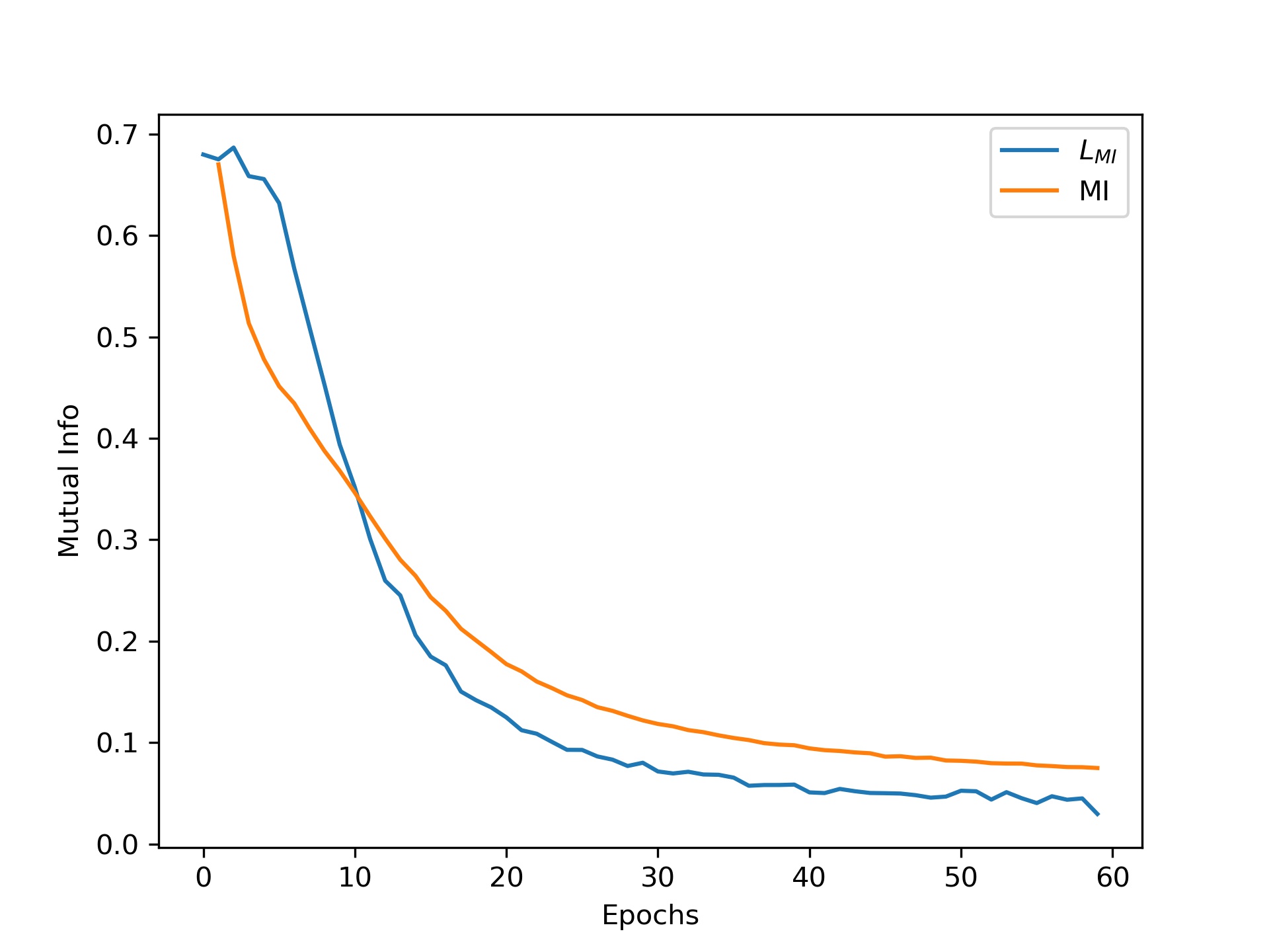
To understand the bi-level objective to MI minimization in Eq. 11, we provide a case study in which we optimize the parameters of distribution to reduce the mutual information between two variables. Consider 333We use the toy dataset from https://github.com/mzgubic/MINE. The distribution of is:
| (18) | ||||
We optimize the parameter to reduce the mutual information between and . For each epoch, we sample 20000 data points from each distribution, denoted as . The inner-step is set to be 150. After the inner optimization ends, the model yields a good mutual information approximator and optimize to reduce the mutual information by minimizing . We compute the mutual information with the traditional method and compare it with :
| (19) | ||||
As is shown in Fig .9, the mutual information decreases as descends. The advantage of such bi-level objective to MI minimization in Eq. 11 is that it only requires samples instead of forms of distribution. Moreover, it needs no tractable prior distribution for variational approximation. The drawback is that it needs additional computation in the inner loop.
A.3 Algorithm
A.4 More results on graph interpretation
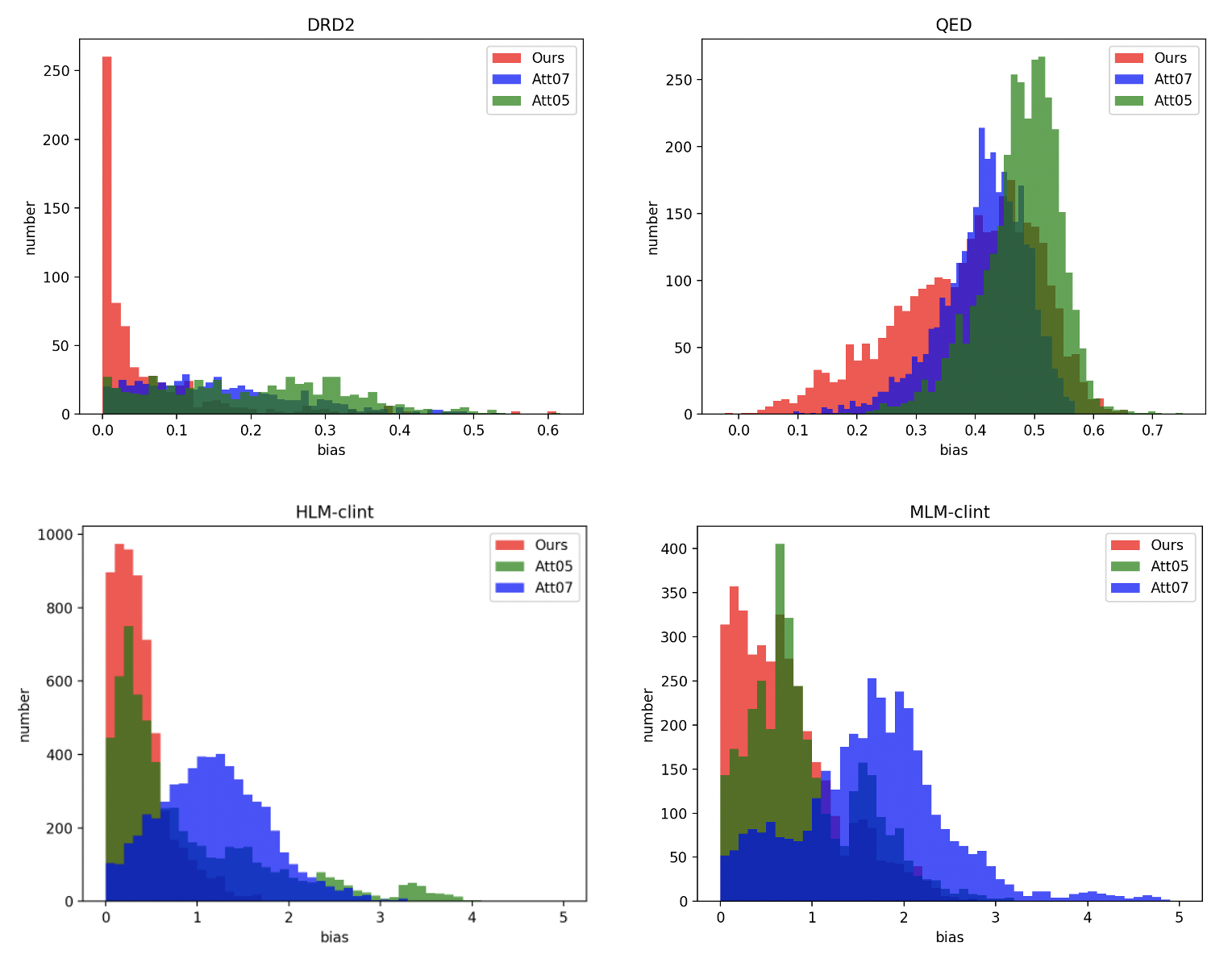
In Fig. 4, we show the distribution of absolute bias between the property of graphs and subgraphs. GIB is able to generate such subgraphs with more similar properties to the original graphs.
In Fig. 5, we provide more results of four properties on graph interpretation.
A.5 More results on noisy graph classification
We provide qualitative results on noisy graph classification in Fig. 6.
