Privacy-Preserving Distributed Projection LMS for Linear Multitask Networks

Chengcheng Wang, , Wee Peng Tay, , Ye Wei, , and Yuan Wang This work was supported in part by the Singapore Ministry of Education Academic Research Fund Tier 2 grant MOE2018-T2-2-019 and by A*STAR under its RIE2020 Advanced Manufacturing and Engineering (AME) Industry Alignment Fund – Pre Positioning (IAF-PP) (Grant No. A19D6a0053).C. Wang, W. P. Tay and Y. Wang are with Nanyang Technological University, Singapore. Y. Wei is with Northeast Electric Power University, China. E-mails: wangcc@ntu.edu.sg; wptay@ntu.edu.sg; weiye@hrbeu.edu.cn; wangyuan@ntu.edu.sg.
Abstract

We develop a privacy-preserving distributed projection least mean squares (LMS) strategy over linear multitask networks, where agents’ local parameters of interest or tasks are linearly related. Each agent is interested in not only improving its local inference performance via in-network cooperation with neighboring agents, but also protecting its own individual task against privacy leakage. In our proposed strategy, at each time instant, each agent sends a noisy estimate, which is its local intermediate estimate corrupted by a zero-mean additive noise, to its neighboring agents. We derive a sufficient condition to determine the amount of noise to add to each agent’s intermediate estimate to achieve an optimal trade-off between the network mean-square-deviation and an inference privacy constraint. We propose a distributed and adaptive strategy to compute the additive noise powers, and study the mean and mean-square behaviors and privacy-preserving performance of the proposed strategy. Simulation results demonstrate that our strategy is able to balance the trade-off between estimation accuracy and privacy preservation.

Index Terms:
Distributed strategies, multitask networks, inference privacy, privacy preservation, additive noises.

I Introduction

In multitask distributed networks, a set of interconnected agents work collaboratively to estimate different but related parameters of interest [1, 2, 3, 4, 5, 6, 7, 8]. In order to make use of the relationship between different tasks for better inference performance, local estimates are exchanged amongst agents within the same neighborhood. However, each agent may wish to protect its own local parameters of interest and prevent other agents in the network from accurately inferring these parameters. For example, in an Internet of Things (IoT) network, sensors are deployed in smart grids, traffic monitoring, health monitoring, home monitoring and other applications [9, 10, 11, 12]. Although different IoT or edge computing devices may have their local objectives, they can exchange information with each other or service providers [13, 14, 15, 16] to improve inferences and services. However, sharing information may lead to privacy leakage.

To protect the privacy of data being exchanged between agents in a distributed network, the works [17, 18, 19, 20, 21, 22] propose local differential privacy mechanisms, while [23, 24, 25, 26] develop privacy-preserving distributed data analytics. However, these approaches often lead to significant trade-offs in estimation accuracy as they do not specifically protect the privacy of the parameters of interest. Privacy-preserving average consensus algorithms in [27, 28, 29, 30, 31] aim to guarantee the privacy of initial states while achieving asymptotic consensus on the average of the initial values. To achieve inference privacy in a decentralized IoT network, [32, 33, 34, 35, 36] propose approaches with information privacy guarantees, while [37, 38, 39, 40, 41, 42, 43] map the agents’ raw observations into a lower dimensional subspace. These inference privacy works assume that all agents in the network are interested in inferring the same parameters or hypothesis of interest.

Existing works on multitask distributed networks mainly focus on developing new distributed strategies for automatic clustering [44, 2] and handling different relationships among the tasks [1, 4, 5, 6, 7, 8]. Other works like [45, 46, 47, 2] focus on evaluating the performance of different distributed schemes. Few works have considered protecting the privacy of each agent’s local parameters. The reference [48] considers data privacy of the agents’ local measurements in a single-task network.

Our objective is to develop a privacy-preserving distributed projection least mean squares (LMS) strategy over multitask networks, which balances the trade-off between estimation accuracy and privacy preservation of agents’ local parameters or tasks. Specifically, we consider multitask estimation problems where the unknown parameters of interest within each neighborhood are linearly related with each other [7]. Such problems exist widely in applications such as electrical networks, telecommunication networks, and pipeline networks. Different from the strategy in [7], which does not take privacy preservation into consideration, we propose to sanitize each agent’s intermediate estimate before sharing it with its neighbors by adding an appropriate zero-mean noise to the intermediate estimate. We study how to design the power of the noise to be added to optimize the trade-off between the network mean-square-deviation (MSD) and the inference privacy of each agent’s local parameters, measured by its neighbors’ mean-square error in estimating the agent’s local parameters. In addition, different from existing works on distributed strategies in the presence of link noises [46, 47, 49, 50], which examine the effect of link noises on the performance of distributed strategies, this work focuses on developing agent-specific time-varying variances of the additive noises that enable agents to benefit from in-network cooperation as well as to protect their own individual tasks against privacy leakage.

The rest of this paper is organized as follows. In Section II, we introduce the system assumptions and the multitask estimation problem considered in this paper. In Section III, we propose a privacy-preserving multitask distributed strategy by introducing privacy noises and show how to obtain the noise powers in Section IV. We examine the mean and mean-square behaviors and privacy-preserving performance of the proposed strategy in Section V. We present simulation results in Section VI. Section VII concludes the paper.

Notations: We use lowercase letters to denote vectors and scalars, uppercase letters for matrices, plain letters for deterministic variables, and boldface letters for random variables. We use ()superscript(\cdot)^{\intercal}, ()1superscript1(\cdot)^{-1}, Tr()Tr{\operatorname{Tr}\left(\cdot\right)} and rank()rank\operatorname{rank}\left(\cdot\right) to denote matrix transpose, inversion, trace and rank, respectively. We use diag{}diag\operatorname{diag}\{\cdot\}, col{}col\operatorname{col}\left\{{\cdot}\right\} and row{}row\operatorname{row}\left\{{\cdot}\right\} for a diagonal matrix, column vector and row vector, respectively. The M×M𝑀𝑀M\times M identity matrix is denoted as IMsubscript𝐼𝑀I_{M} and 0M×Nsubscript0𝑀𝑁0_{M\times N} denotes an M×N𝑀𝑁M\times N zero matrix. We have xΣ2=xΣxsubscriptsuperscriptdelimited-∥∥𝑥2Σsuperscript𝑥Σ𝑥{\left\lVert{x}\right\rVert}^{2}_{\Sigma}=x^{\intercal}\Sigma x with ΣΣ\Sigma being a symmetric positive semidefinite matrix, and let x2=xIM2superscriptdelimited-∥∥𝑥2superscriptsubscriptdelimited-∥∥𝑥subscript𝐼𝑀2{\left\lVert{x}\right\rVert}^{2}={\left\lVert{x}\right\rVert}_{I_{M}}^{2} where M𝑀M is the length of x𝑥x. In addition, we use ρ(A)𝜌𝐴\rho(A) to denote the spectral radius of matrix A𝐴A, and λmin(A)subscript𝜆𝐴\lambda_{\min}(A) and λmax(A)subscript𝜆𝐴\lambda_{\max}(A) for the minimum and maximum eigenvalues of the symmetric matrix A𝐴A, respectively. For a block matrix A𝐴A whose (k,)𝑘(k,\ell)-th block represents some interaction between agents k𝑘k and \ell, we let [A]ksubscriptdelimited-[]𝐴𝑘[A]_{k} and [A],ksubscriptdelimited-[]𝐴𝑘[A]_{\cdot,k} denote the block row and block column of A𝐴A corresponding to agent k𝑘k, respectively, and [A]k,subscriptdelimited-[]𝐴𝑘[A]_{k,\ell} be the (k,)𝑘(k,\ell)-th block.

II Linear Multitask Networks

In this section, we present our system model, and give a brief introduction to multitask networks, where neighboring agents’ tasks are linearly related. Consider a strongly-connected network of N𝑁N agents, where information can flow in either direction between any two connected agents [46]. At each time instant i0𝑖0i\geq 0, each agent k𝑘k has access to a scalar observation 𝒅k(i)subscript𝒅𝑘𝑖{\bm{d}}_{k}(i), and an Mk×1subscript𝑀𝑘1M_{k}\times 1 regression vector 𝒖k(i)subscript𝒖𝑘𝑖{\bm{u}}_{k}(i). The random data {𝒅k(i),𝒖k(i)}subscript𝒅𝑘𝑖subscript𝒖𝑘𝑖\{\bm{d}_{k}(i),\bm{u}_{k}(i)\} are related via the linear regression model

𝒅k(i)=𝒖k(i)𝒘ko+𝒗k(i)subscript𝒅𝑘𝑖superscriptsubscript𝒖𝑘𝑖superscriptsubscript𝒘𝑘𝑜subscript𝒗𝑘𝑖\displaystyle{\bm{d}}_{k}(i)={\bm{u}}_{k}^{\intercal}(i){\bm{w}}_{k}^{o}+{\bm{v}}_{k}(i) (1)

where the scalar 𝒗k(i)subscript𝒗𝑘𝑖\bm{v}_{k}(i) is measurement noise, 𝒘kosuperscriptsubscript𝒘𝑘𝑜{\bm{w}}_{k}^{o} is an Mk×1subscript𝑀𝑘1M_{k}\times 1 unknown random vector, with mean 𝔼𝒘ko𝔼superscriptsubscript𝒘𝑘𝑜\mathbb{E}{\bm{w}}_{k}^{o} and covariance matrix

Wkk=𝔼[(𝒘ko𝔼𝒘ko)(𝒘ko𝔼𝒘ko)]subscript𝑊𝑘𝑘𝔼delimited-[]subscriptsuperscript𝒘𝑜𝑘𝔼subscriptsuperscript𝒘𝑜𝑘superscriptsubscriptsuperscript𝒘𝑜𝑘𝔼subscriptsuperscript𝒘𝑜𝑘\displaystyle W_{kk}=\mathbb{E}\left[{({\bm{w}}^{o}_{k}-\mathbb{E}{\bm{w}}^{o}_{k})({\bm{w}}^{o}_{k}-\mathbb{E}{\bm{w}}^{o}_{k})^{\intercal}}\right]

Although we assume that the parameter vector 𝒘kosuperscriptsubscript𝒘𝑘𝑜{\bm{w}}_{k}^{o} is random instead of being a deterministic parameter vector, like most of the literature on distributed strategies [2, 6, 1, 45, 48, 49, 47, 7, 5, 4, 51, 44, 50, 46], we assume that the parameter vector 𝒘kosuperscriptsubscript𝒘𝑘𝑜{\bm{w}}_{k}^{o} is fixed at a certain realization wkosuperscriptsubscript𝑤𝑘𝑜w_{k}^{o} during the distributed estimation process. Since our goal is to develop inference privacy mechanisms that lead to high estimation errors, on average, of agent k𝑘k’s local parameters 𝒘kosuperscriptsubscript𝒘𝑘𝑜{\bm{w}}_{k}^{o} by other agents k𝑘\ell\neq k, we adopt a Bayesian framework for the privacy criterion.

We make the following assumptions regarding model (1).

Assumption 1.

(Measurement noise) The measurement noise 𝐯k(i)subscript𝐯𝑘𝑖\bm{v}_{k}(i) is white over time, with zero mean, and a variance of σv,k2superscriptsubscript𝜎𝑣𝑘2\sigma_{v,k}^{2}.

Assumption 2.

(Regressors) The regressors {𝐮k(i)}subscript𝐮𝑘𝑖\{\bm{u}_{k}(i)\} are zero-mean, white over time and space with

𝔼𝒖k(i)𝒖(j)=Ru,kδk,δi,j,𝔼subscript𝒖𝑘𝑖superscriptsubscript𝒖𝑗subscript𝑅𝑢𝑘subscript𝛿𝑘subscript𝛿𝑖𝑗\displaystyle\mathbb{E}\bm{u}_{k}(i)\bm{u}_{\ell}^{\intercal}(j)=R_{u,k}\delta_{k,\ell}\delta_{i,j}, (2)

where Ru,ksubscript𝑅𝑢𝑘R_{u,k} is symmetric positive definite, and δk,subscript𝛿𝑘\delta_{k,\ell} is the Kronecker delta.

Assumption 3.

(Independence) The random data {𝐰ko,𝐮(i),𝐯m(j)}superscriptsubscript𝐰𝑘𝑜subscript𝐮𝑖subscript𝐯𝑚𝑗\{{\bm{w}}_{k}^{o},{\bm{u}}_{\ell}(i),{\bm{v}}_{m}(j)\} are independent of each other for any agents k,,m𝑘𝑚k,\ell,m and any time instants i,j𝑖𝑗i,j.

For a realization {𝒘ko=wkok=1,,N}conditional-setsuperscriptsubscript𝒘𝑘𝑜superscriptsubscript𝑤𝑘𝑜𝑘1𝑁\{{\bm{w}}_{k}^{o}=w_{k}^{o}\mid k=1,\ldots,N\}, the objective of each agent k𝑘k is to find the minimizer of the following mean-square-error cost function:

Jk(wk)=𝔼[(𝒅k(i)𝒖k(i)wk)2|𝒘ko=wko]\displaystyle J_{k}(w_{k})=\mathbb{E}\left[{({\bm{d}}_{k}(i)-{\bm{u}}_{k}^{\intercal}(i)w_{k})^{2}}\,\middle|\,{{\bm{w}}_{k}^{o}=w_{k}^{o}}\right]

Let 𝒩ksubscript𝒩𝑘\mathcal{N}_{k} be the set of all neighbors of agent k𝑘k, including agent k𝑘k itself, and

𝒘𝒩ko=col{𝒘o}𝒩k.\displaystyle{\bm{w}}_{\mathcal{N}_{k}}^{o}=\operatorname{col}\left\{{{\bm{w}}_{\ell}^{o}}\right\}_{\ell\in\mathcal{N}_{k}}.

Following [7], we assume that neighboring tasks {𝒘o𝒩k}conditional-setsuperscriptsubscript𝒘𝑜subscript𝒩𝑘\{{\bm{w}}_{\ell}^{o}\mid\ell\in\mathcal{N}_{k}\} are related via

𝒟k𝒘𝒩ko+bk=0,subscript𝒟𝑘subscriptsuperscript𝒘𝑜subscript𝒩𝑘subscript𝑏𝑘0\displaystyle\mathcal{D}_{k}{\bm{w}}^{o}_{\mathcal{N}_{k}}+b_{k}=0, (3)

where the matrix 𝒟ksubscript𝒟𝑘\mathcal{D}_{k} is a jk×|𝒩k|subscript𝑗𝑘subscript𝒩𝑘j_{k}\times|\mathcal{N}_{k}| block matrix, and the vector bksubscript𝑏𝑘b_{k} is a jk×1subscript𝑗𝑘1j_{k}\times 1 block vector, with jk1subscript𝑗𝑘1j_{k}\geq 1. Then, the objective for the entire network is to find the optimal solution to the following constrained optimization problem [7]:

minw1,,wNsubscriptsubscript𝑤1subscript𝑤𝑁\displaystyle\min_{w_{1},\ldots,w_{N}}\ k=1NJk(wk)superscriptsubscript𝑘1𝑁subscript𝐽𝑘subscript𝑤𝑘\displaystyle\sum_{k=1}^{N}J_{k}(w_{k}) (4a)
s.t.\displaystyle\operatorname{s.t.}\ w𝒩k=col{w}𝒩k,\displaystyle w_{\mathcal{N}_{k}}=\operatorname{col}\left\{{w_{\ell}}\right\}_{\ell\in\mathcal{N}_{k}}, (4b)
𝒟kw𝒩k+bk=0,for k=1,,N,subscript𝒟𝑘subscript𝑤subscript𝒩𝑘subscript𝑏𝑘0for k=1,,N,\displaystyle\mathcal{D}_{k}w_{\mathcal{N}_{k}}+b_{k}=0,\ \text{for $k=1,\ldots,N$,} (4c)

where individual costs {Jk(wk)}subscript𝐽𝑘subscript𝑤𝑘\{J_{k}(w_{k})\} are defined by Section II. We assume that the optimization problem 4 is feasible [7]. We assume that the matrix 𝒟ksubscript𝒟𝑘\mathcal{D}_{k} for any agent k𝑘k is full row-rank so that the linear equation 4c has at least one solution. To avoid having a trivial solution, we also assume that it is column-rank deficient because otherwise 4c has a unique solution.

As demonstrated in [7], each agent k𝑘k benefits through cooperation with neighboring agents by sharing its local parameter estimate 𝝍k(i)subscript𝝍𝑘𝑖\bm{\psi}_{k}(i) with its neighbors at each time instant i𝑖i. By leveraging the linear relationships 3 and its neighbors’ parameter estimates, an agent can improve its own inference accuracy. In this paper, we consider the scenario where agent k𝑘k also wants to prevent other agents from inferring its own task 𝒘kosuperscriptsubscript𝒘𝑘𝑜{\bm{w}}_{k}^{o}. Thus, a privacy-preserving distributed solution is required to balance the trade-off between estimation accuracy and privacy protection of the individual tasks. In order to limit privacy leakage, we add a zero-mean, independent and identically distributed (i.i.d.) noise vector 𝒏k(i)subscript𝒏𝑘𝑖\bm{n}_{k}(i) to agent k𝑘k’s local parameter estimate 𝝍k(i)subscript𝝍𝑘𝑖\bm{\psi}_{k}(i), which is a local linear estimate of 𝒘kosuperscriptsubscript𝒘𝑘𝑜{\bm{w}}_{k}^{o} (cf. 11, 10 and 7), before communicating 𝝍k(i)=𝝍k(i)+𝒏k(i)subscriptsuperscript𝝍𝑘𝑖subscript𝝍𝑘𝑖subscript𝒏𝑘𝑖\bm{\psi}^{\prime}_{k}(i)=\bm{\psi}_{k}(i)+{\bm{n}_{k}}(i) to neighboring agents. Let σn,k2(i)superscriptsubscript𝜎𝑛𝑘2𝑖\sigma_{n,k}^{2}(i) be the variance of each random entry in 𝒏k(i)subscript𝒏𝑘𝑖\bm{n}_{k}(i). We call 𝒏k(i)subscript𝒏𝑘𝑖{\bm{n}}_{k}(i) a privacy noise.

Our objective is to find the optimal solution to the following optimization problem:

minσn,12(i),,σn,N2(i)subscriptsuperscriptsubscript𝜎𝑛12𝑖superscriptsubscript𝜎𝑛𝑁2𝑖\displaystyle\min_{\sigma_{n,1}^{2}(i),\ldots,\sigma_{n,N}^{2}(i)}\ MSDnet(i)=1Nk=1N𝔼𝒘ko𝒘k(i)2,subscriptMSDnet𝑖1𝑁superscriptsubscript𝑘1𝑁𝔼superscriptdelimited-∥∥superscriptsubscript𝒘𝑘𝑜subscript𝒘𝑘𝑖2\displaystyle\ {\mbox{MSD}}_{\mbox{net}}(i)=\frac{1}{N}\sum_{k=1}^{N}\mathbb{E}{\left\lVert{{\bm{w}}_{k}^{o}-{\bm{w}}_{k}(i)}\right\rVert}^{2}, (5a)
s.t.\displaystyle\operatorname{s.t.}\ 𝔼𝒘ko𝒘^k|𝝍k(i)2δk,𝔼superscriptdelimited-∥∥superscriptsubscript𝒘𝑘𝑜subscript^𝒘conditional𝑘subscriptsuperscript𝝍𝑘𝑖2subscript𝛿𝑘\displaystyle\ \mathbb{E}{\left\lVert{{\bm{w}}_{k}^{o}-\widehat{{\bm{w}}}_{k|\bm{\psi}^{\prime}_{k}}(i)}\right\rVert}^{2}\geq\delta_{k}, (5b)

for k=1,,N,i0formulae-sequence𝑘1𝑁𝑖0k=1,\ldots,N,i\geq 0, and where 𝒘^k|𝝍k(i)subscript^𝒘conditional𝑘subscriptsuperscript𝝍𝑘𝑖\widehat{{\bm{w}}}_{k|\bm{\psi}^{\prime}_{k}}(i) is the least mean-square estimate of 𝒘kosuperscriptsubscript𝒘𝑘𝑜{\bm{w}}_{k}^{o} at time instant i𝑖i based on 𝝍k(i)subscriptsuperscript𝝍𝑘𝑖\bm{\psi}^{\prime}_{k}(i), and δk0subscript𝛿𝑘0\delta_{k}\geq 0 is a privacy threshold chosen according to privacy requirements. Note that the privacy thresholds have to be chosen such that

0δkTr(Wkk),0subscript𝛿𝑘Trsubscript𝑊𝑘𝑘\displaystyle 0\leq\delta_{k}\leq{\operatorname{Tr}\left(W_{kk}\right)}, (6)

otherwise 5 is infeasible.

  • Remark 1: 

    In 5b, it is required that at each time instant i0𝑖0i\geq 0, the expected squared distance 𝔼𝒘ko𝒘^k|𝝍k(i)2𝔼superscriptdelimited-∥∥superscriptsubscript𝒘𝑘𝑜subscript^𝒘conditional𝑘subscriptsuperscript𝝍𝑘𝑖2\mathbb{E}{\left\lVert{{\bm{w}}_{k}^{o}-\widehat{{\bm{w}}}_{k|\bm{\psi}^{\prime}_{k}}(i)}\right\rVert}^{2} over all realizations of 𝒘kosuperscriptsubscript𝒘𝑘𝑜{\bm{w}}_{k}^{o} is no smaller than the predefined parameter δksubscript𝛿𝑘\delta_{k}. This provides an inference privacy constraint on the ability of a neighboring agent to agent k𝑘k in accurately estimating 𝒘kosuperscriptsubscript𝒘𝑘𝑜{\bm{w}}_{k}^{o} based on observation 𝝍k(i)subscriptsuperscript𝝍𝑘𝑖\bm{\psi}^{\prime}_{k}(i) on average.

  • Remark 2: 

    In 5b, the estimator 𝒘^k|𝝍k(i)subscript^𝒘conditional𝑘subscriptsuperscript𝝍𝑘𝑖\widehat{{\bm{w}}}_{k|\bm{\psi}^{\prime}_{k}}(i) is based only on the noisy estimate 𝝍k(i)subscriptsuperscript𝝍𝑘𝑖\bm{\psi}^{\prime}_{k}(i). For each neighboring agent 𝒩ksubscript𝒩𝑘\ell\in\mathcal{N}_{k}, it has access to not only the received noisy estimate 𝝍k(i)subscriptsuperscript𝝍𝑘𝑖\bm{\psi}^{\prime}_{k}(i) from agent k𝑘k, but also its own intermediate estimate 𝝍(i)subscript𝝍𝑖\bm{\psi}_{\ell}(i) of 𝒘osuperscriptsubscript𝒘𝑜{\bm{w}}_{\ell}^{o}. Both of these estimates can be used to infer 𝒘kosuperscriptsubscript𝒘𝑘𝑜{\bm{w}}_{k}^{o} as the unknown parameters 𝒘kosuperscriptsubscript𝒘𝑘𝑜{\bm{w}}_{k}^{o} and 𝒘osuperscriptsubscript𝒘𝑜{\bm{w}}_{\ell}^{o} are linearly related with each other through 4c. In this paper, to simplify the analysis and to ensure that the sequence of noise variances {σn,k2(i)}superscriptsubscript𝜎𝑛𝑘2𝑖\{\sigma_{n,k}^{2}(i)\} at each agent k𝑘k is bounded and convergent, we only consider the simplified case in 5. We illustrate the case where a neighboring agent uses its own estimates as additional information using simulations in Section VI.

III Privacy-preserving Distributed Projection LMS

In this section, we propose an inference privacy mechanism to protect each agent’s local task by adding noise to its intermediate estimate before sharing with its neighbors. We then introduce a weighted projection operator, which projects neighbors’ noisy estimates onto the linear manifold defined by local constraints (3), in order to mitigate the negative effect of the additive noises on the estimation accuracy of individual tasks.

III-A Adapt-Then-Project Strategy

In our privacy-preserving distributed projection LMS algorithm, we initialize 𝒘k(1)=0subscript𝒘𝑘10\bm{w}_{k}(-1)=0 for every agent k𝑘k in the network. Given data {𝒅k(i),𝒖k(i)}subscript𝒅𝑘𝑖subscript𝒖𝑘𝑖\{\bm{d}_{k}(i),\bm{u}_{k}(i)\} for each time instant i0𝑖0i\geq 0, and for each agent k=1,,N𝑘1𝑁k=1,\ldots,N, we perform the following steps iteratively:

  1. 1.

    Adaptation. Each agent k𝑘k updates its current estimate 𝒘k(i1)subscript𝒘𝑘𝑖1\bm{w}_{k}(i-1) using the stochastic gradient descent (SGD) algorithm to obtain an intermediate estimate

    𝝍k(i)=𝒘k(i1)+μk𝒖k(i)(𝒅k(i)𝒖k(i)𝒘k(i1)),subscript𝝍𝑘𝑖subscript𝒘𝑘𝑖1subscript𝜇𝑘subscript𝒖𝑘𝑖subscript𝒅𝑘𝑖subscriptsuperscript𝒖𝑘𝑖subscript𝒘𝑘𝑖1\displaystyle\bm{\psi}_{k}(i)=\bm{w}_{k}(i-1)\!+\!\mu_{k}\bm{u}_{k}(i)\left(\bm{d}_{k}(i)\!-\!\bm{u}^{\intercal}_{k}(i)\bm{w}_{k}(i-1)\right), (7)

    where μk>0subscript𝜇𝑘0\mu_{k}>0 is the step size at agent k𝑘k.

  2. 2.

    Exchange. Each agent k𝑘k sends a noisy estimate

    𝝍k(i)=𝝍k(i)+𝒏k(i),subscriptsuperscript𝝍𝑘𝑖subscript𝝍𝑘𝑖subscript𝒏𝑘𝑖\displaystyle\bm{\psi}^{\prime}_{k}(i)=\bm{\psi}_{k}(i)+\bm{n}_{k}(i),

    where the random additive noise vector 𝒏k(i)subscript𝒏𝑘𝑖{\bm{n}}_{k}(i) is of dimension Mk×1subscript𝑀𝑘1M_{k}\times 1, to its neighbors and collects estimates {𝝍(i)}subscriptsuperscript𝝍𝑖\{\bm{\psi}^{\prime}_{\ell}(i)\} from neighboring agents {𝒩k}subscript𝒩𝑘\{\ell\in\mathcal{N}_{k}\}:

    𝝍(i)={𝝍(i)+𝒏(i),if 𝒩k\{k},𝝍k(i),if =k.subscriptsuperscript𝝍𝑖casessubscript𝝍𝑖subscript𝒏𝑖if 𝒩k\{k}subscript𝝍𝑘𝑖if =k\displaystyle\bm{\psi}^{\prime}_{\ell}(i)=\left\{\begin{array}[]{ll}\bm{\psi}_{\ell}(i)+\bm{n}_{\ell}(i),&\textrm{if $\ell\in\mathcal{N}_{k}\backslash\{k\}$},\\ \bm{\psi}_{k}(i),&\textrm{if $\ell=k$}.\end{array}\right. (10)
  3. 3.

    Projection. Each agent k𝑘k projects the estimates {𝝍(i)}𝒩ksubscriptsubscriptsuperscript𝝍𝑖subscript𝒩𝑘\{\bm{\psi}^{\prime}_{\ell}(i)\}_{\ell\in\mathcal{N}_{k}} received from its neighborhood onto the linear manifold {w𝒩k𝒟kw𝒩k+bk=0}conditional-setsubscript𝑤subscript𝒩𝑘subscript𝒟𝑘subscript𝑤subscript𝒩𝑘subscript𝑏𝑘0\{w_{\mathcal{N}_{k}}\mid\mathcal{D}_{k}w_{\mathcal{N}_{k}}+b_{k}=0\} to obtain

    𝒘k(i)=[𝒫𝒩k(i)]kcol{𝝍(i)}𝒩k[f𝒩k(i)]k,\displaystyle{\bm{w}}_{k}(i)=[\mathcal{P}_{\mathcal{N}_{k}}(i)]_{k}\operatorname{col}\left\{{\bm{\psi}^{\prime}_{\ell}(i)}\right\}_{\ell\in\mathcal{N}_{k}}-[f_{\mathcal{N}_{k}}(i)]_{k}, (11)

    where the matrix 𝒫𝒩k(i)subscript𝒫subscript𝒩𝑘𝑖\mathcal{P}_{\mathcal{N}_{k}}(i) and vector f𝒩k(i)subscript𝑓subscript𝒩𝑘𝑖f_{\mathcal{N}_{k}}(i) are defined in 16 and 15, respectively, in the sequel.

Let δ=col{δk}k=1N\delta=\operatorname{col}\left\{{\delta_{k}}\right\}_{k=1}^{N}, where the non-negative numbers {δk}subscript𝛿𝑘\{\delta_{k}\} are the privacy thresholds in 5b. We call the proposed scheme 7, 10 and 11 adapt-then-project with privacy parameter δ𝛿\delta or ATP(δ)𝛿(\delta) in short. Specifically, we use ATP(0) algorithm to denote the case where there is no privacy constraint, i.e., no additive noises are introduced in the exchange step in 10.

  • Remark 3: 

    The differences between the proposed ATP(δ)𝛿(\delta) algorithm 7, 11 and 10 and the scheme in [7] are in the exchange and projection steps. Specifically, in order to protect each individual task 𝒘kosuperscriptsubscript𝒘𝑘𝑜{\bm{w}}_{k}^{o} against privacy leakage, each agent k𝑘k sends a noisy intermediate estimate 𝝍k(i)subscriptsuperscript𝝍𝑘𝑖\bm{\psi}^{\prime}_{k}(i), instead of the true estimate 𝝍k(i)subscript𝝍𝑘𝑖\bm{\psi}_{k}(i) as in [7], to its neighboring agents. In addition, in the projection step 11, agent k𝑘k projects its neighboring estimates onto the linear manifold corresponding to the intersection of all jksubscript𝑗𝑘j_{k} linear equality constraints that it is involved in. In contrast, in [7], neighboring estimates of agent k𝑘k are projected onto the linear manifold corresponding to each of the jksubscript𝑗𝑘j_{k} constraints separately, which generates jksubscript𝑗𝑘j_{k} intermediate estimates, and the new estimate is taken as the average of these intermediate estimates. Moreover, in order to mitigate the negative effect of privacy noises on the projection step, we introduce weighted projection operators in 12 in the sequel.

To allow a distributed implementation of the privacy mechanism, we make the following assumption.

Assumption 4.

(Privacy noise) The entries of 𝐧k(i)subscript𝐧𝑘𝑖{\bm{n}}_{k}(i) at time instant i𝑖i, for any k=1,,N𝑘1𝑁k=1,\ldots,N, are i.i.d. with zero mean and variance σn,k2(i)superscriptsubscript𝜎𝑛𝑘2𝑖\sigma_{n,k}^{2}(i), i.e.,

Rn,k(i)𝔼[𝒏k(i)𝒏k(i)]=σn,k2(i)IMksubscript𝑅𝑛𝑘𝑖𝔼delimited-[]subscript𝒏𝑘𝑖superscriptsubscript𝒏𝑘𝑖superscriptsubscript𝜎𝑛𝑘2𝑖subscript𝐼subscript𝑀𝑘\displaystyle R_{n,k}(i)\triangleq\mathbb{E}\left[{{\bm{n}}_{k}(i){\bm{n}}_{k}^{\intercal}(i)}\right]=\sigma_{n,k}^{2}(i)I_{M_{k}}

The random noises {𝐧k(i)}subscript𝐧𝑘𝑖\{{\bm{n}}_{k}(i)\} are white over time and space. The random process {𝐧k(i)}subscript𝐧𝑘𝑖\{{\bm{n}}_{k}(i)\} is independent of any other random processes. From Assumption 4, each agent k𝑘k generates the noise 𝐧k(i)subscript𝐧𝑘𝑖{\bm{n}}_{k}(i) independently of other agents in the network, and also independently over time instants i0𝑖0i\geq 0. Based on this assumption, we now proceed to introduce the weighted projection operator 𝒫𝒩k(i)subscript𝒫subscript𝒩𝑘𝑖\mathcal{P}_{\mathcal{N}_{k}}(i) and vector f𝒩k(i)subscript𝑓subscript𝒩𝑘𝑖f_{\mathcal{N}_{k}}(i) involved in 11.

III-B Weighted Projection Operator

For each agent k𝑘k, let us collect the noisy intermediate estimates {𝝍(i)}subscriptsuperscript𝝍𝑖\{\bm{\psi}^{\prime}_{\ell}(i)\} defined by 10 from its neighboring agents {𝒩k}subscript𝒩𝑘\{\ell\in\mathcal{N}_{k}\} into an |𝒩k|×1subscript𝒩𝑘1|\mathcal{N}_{k}|\times 1 block column vector

𝝍𝒩k(i)=col{𝝍(i)}𝒩k.\displaystyle\bm{\psi}^{\prime}_{\mathcal{N}_{k}}(i)=\operatorname{col}\left\{{\bm{\psi}^{\prime}_{\ell}(i)}\right\}_{\ell\in\mathcal{N}_{k}}.

Then, for each random realization 𝝍𝒩k(i)=ψ𝒩k(i)subscriptsuperscript𝝍subscript𝒩𝑘𝑖subscriptsuperscript𝜓subscript𝒩𝑘𝑖\bm{\psi}^{\prime}_{\mathcal{N}_{k}}(i)=\psi^{\prime}_{\mathcal{N}_{k}}(i), we are interested in seeking the optimal solution to the following optimization problem:

minw𝒩k(i)subscriptsubscript𝑤subscript𝒩𝑘𝑖\displaystyle\min_{w_{\mathcal{N}_{k}}(i)}\ ψ𝒩k(i)w𝒩k(i)Ω𝒩k1(i)2subscriptsuperscriptdelimited-∥∥subscriptsuperscript𝜓subscript𝒩𝑘𝑖subscript𝑤subscript𝒩𝑘𝑖2superscriptsubscriptΩsubscript𝒩𝑘1𝑖\displaystyle{\left\lVert{\psi^{\prime}_{\mathcal{N}_{k}}(i)-w_{\mathcal{N}_{k}}(i)}\right\rVert}^{2}_{\Omega_{\mathcal{N}_{k}}^{-1}(i)} (12a)
s.t.\displaystyle\operatorname{s.t.}\ 𝒟kw𝒩k(i)+bk=0,subscript𝒟𝑘subscript𝑤subscript𝒩𝑘𝑖subscript𝑏𝑘0\displaystyle\mathcal{D}_{k}w_{\mathcal{N}_{k}}(i)+b_{k}=0, (12b)

where the weight matrix

Ω𝒩k1(i)=diag{ωk(i)IM}𝒩k,\displaystyle\Omega_{\mathcal{N}_{k}}^{-1}(i)=\operatorname{diag}\left\{\omega_{\ell k}(i)I_{M_{\ell}}\right\}_{\ell\in\mathcal{N}_{k}}, (13)

with

ωk(i)>0for 𝒩k, and𝒩kωk(i)=1.subscript𝜔𝑘𝑖0for 𝒩k, andsubscriptsubscript𝒩𝑘subscript𝜔𝑘𝑖1\displaystyle\omega_{\ell k}(i)>0\,\textrm{for $\ell\in\mathcal{N}_{k}$, and}\sum_{\ell\in\mathcal{N}_{k}}\omega_{\ell k}(i)=1. (14)

We note that Ω𝒩k1(i)superscriptsubscriptΩsubscript𝒩𝑘1𝑖\Omega_{\mathcal{N}_{k}}^{-1}(i) is an |𝒩k|×|𝒩k|subscript𝒩𝑘subscript𝒩𝑘|\mathcal{N}_{k}|\times|\mathcal{N}_{k}| block-diagonal, symmetric and positive definite matrix. We assume that the weights {ωk(i)}subscript𝜔𝑘𝑖\{\omega_{\ell k}(i)\} defined by 13 converge as i𝑖i\to\infty. Let

M𝒩k=𝒩kM,subscript𝑀subscript𝒩𝑘subscriptsubscript𝒩𝑘subscript𝑀\displaystyle M_{\mathcal{N}_{k}}=\sum_{\ell\in\mathcal{N}_{k}}M_{\ell},

and

𝒫𝒩k(i)subscript𝒫subscript𝒩𝑘𝑖\displaystyle\mathcal{P}_{\mathcal{N}_{k}}(i) =IM𝒩kΩ𝒩k(i)𝒟k(𝒟kΩ𝒩k(i)𝒟k)1𝒟kabsentsubscript𝐼subscript𝑀subscript𝒩𝑘subscriptΩsubscript𝒩𝑘𝑖superscriptsubscript𝒟𝑘superscriptsubscript𝒟𝑘subscriptΩsubscript𝒩𝑘𝑖superscriptsubscript𝒟𝑘1subscript𝒟𝑘\displaystyle=I_{M_{\mathcal{N}_{k}}}-\Omega_{\mathcal{N}_{k}}(i)\mathcal{D}_{k}^{\intercal}(\mathcal{D}_{k}\Omega_{\mathcal{N}_{k}}(i)\mathcal{D}_{k}^{\intercal})^{-1}\mathcal{D}_{k} (15)
f𝒩k(i)subscript𝑓subscript𝒩𝑘𝑖\displaystyle f_{\mathcal{N}_{k}}(i) =Ω𝒩k(i)𝒟k(𝒟kΩ𝒩k(i)𝒟k)1bk.absentsubscriptΩsubscript𝒩𝑘𝑖superscriptsubscript𝒟𝑘superscriptsubscript𝒟𝑘subscriptΩsubscript𝒩𝑘𝑖superscriptsubscript𝒟𝑘1subscript𝑏𝑘\displaystyle=\Omega_{\mathcal{N}_{k}}(i)\mathcal{D}_{k}^{\intercal}(\mathcal{D}_{k}\Omega_{\mathcal{N}_{k}}(i)\mathcal{D}_{k}^{\intercal})^{-1}b_{k}. (16)

It follows that matrix 𝒫𝒩k(i)subscript𝒫subscript𝒩𝑘𝑖\mathcal{P}_{\mathcal{N}_{k}}(i) is a projection matrix. From [52], the minimizer of 12 is given by

w𝒩k(i)=𝒫𝒩k(i)ψ𝒩k(i)f𝒩k(i).subscript𝑤subscript𝒩𝑘𝑖subscript𝒫subscript𝒩𝑘𝑖subscriptsuperscript𝜓subscript𝒩𝑘𝑖subscript𝑓subscript𝒩𝑘𝑖\displaystyle w_{\mathcal{N}_{k}}(i)=\mathcal{P}_{\mathcal{N}_{k}}(i)\psi^{\prime}_{\mathcal{N}_{k}}(i)-f_{\mathcal{N}_{k}}(i). (17)

For each 𝒩ksubscript𝒩𝑘\ell\in\mathcal{N}_{k}, we are interested in the projection operator applied to the intermediate estimate from agent \ell. This corresponds to an Mk×Msubscript𝑀𝑘subscript𝑀M_{k}\times M_{\ell} block of 𝒫𝒩k(i)subscript𝒫subscript𝒩𝑘𝑖\mathcal{P}_{\mathcal{N}_{k}}(i), denoted as [𝒫𝒩k(i)]k,subscriptdelimited-[]subscript𝒫subscript𝒩𝑘𝑖𝑘[\mathcal{P}_{\mathcal{N}_{k}}(i)]_{k,\ell}. We collect all these in an N×N𝑁𝑁N\times N block matrix 𝒫(i)𝒫𝑖\mathcal{P}(i), whose Mk×Msubscript𝑀𝑘subscript𝑀M_{k}\times M_{\ell} (k,)𝑘(k,\ell)-th block equals

[𝒫(i)]k,={[𝒫𝒩k(i)]k,,if 𝒩k,0Mk×M,otherwise.subscriptdelimited-[]𝒫𝑖𝑘casessubscriptdelimited-[]subscript𝒫subscript𝒩𝑘𝑖𝑘if 𝒩ksubscript0subscript𝑀𝑘subscript𝑀otherwise\displaystyle[\mathcal{P}(i)]_{k,\ell}=\left\{\begin{array}[]{ll}\left[\mathcal{P}_{\mathcal{N}_{k}}(i)\right]_{k,\ell},&\textrm{if $\ell\in\mathcal{N}_{k}$},\\ 0_{M_{k}\times M_{\ell}},&\textrm{otherwise}.\end{array}\right. (20)

Similarly, we collect the block [f𝒩k(i)]ksubscriptdelimited-[]subscript𝑓subscript𝒩𝑘𝑖𝑘[f_{\mathcal{N}_{k}}(i)]_{k} corresponding to agent k𝑘k and define an N×1𝑁1N\times 1 block vector

f(i)=col{[f𝒩k(i)]k}k=1N.\displaystyle f(i)=\operatorname{col}\left\{{[f_{\mathcal{N}_{k}}(i)]_{k}}\right\}_{k=1}^{N}. (21)

III-C Weight Matrix

The matrix Ω𝒩k1(i)superscriptsubscriptΩsubscript𝒩𝑘1𝑖\Omega_{\mathcal{N}_{k}}^{-1}(i) is introduced in order to mitigate the negative effect of the privacy noises {𝒏k(i)}subscript𝒏𝑘𝑖\{{\bm{n}}_{k}(i)\} on the projection step 11. In the special case where

Ω𝒩k1(i)=diag{1|𝒩k|IM}𝒩k,\displaystyle\Omega_{\mathcal{N}_{k}}^{-1}(i)=\operatorname{diag}\left\{\frac{1}{|\mathcal{N}_{k}|}I_{M_{\ell}}\right\}_{\ell\in\mathcal{N}_{k}},

the optimal solution of 12 is reduced to the Euclidean projection of ψ𝒩k(i)subscriptsuperscript𝜓subscript𝒩𝑘𝑖\psi^{\prime}_{\mathcal{N}_{k}}(i) on the affine set {w𝒩k𝒟kw𝒩k+bk=0}conditional-setsubscript𝑤subscript𝒩𝑘subscript𝒟𝑘subscript𝑤subscript𝒩𝑘subscript𝑏𝑘0\left\{w_{\mathcal{N}_{k}}\mid\mathcal{D}_{k}w_{\mathcal{N}_{k}}+b_{k}=0\right\} [53, p.398]. We proceed to rewrite 12a as

ψ𝒩k(i)w𝒩k(i)Ω𝒩k1(i)2=𝒩kωk(i)ψ(i)w(i)2.subscriptsuperscriptdelimited-∥∥subscriptsuperscript𝜓subscript𝒩𝑘𝑖subscript𝑤subscript𝒩𝑘𝑖2superscriptsubscriptΩsubscript𝒩𝑘1𝑖subscriptsubscript𝒩𝑘subscript𝜔𝑘𝑖superscriptdelimited-∥∥subscriptsuperscript𝜓𝑖subscript𝑤𝑖2\displaystyle{\left\lVert{\psi^{\prime}_{\mathcal{N}_{k}}(i)-w_{\mathcal{N}_{k}}(i)}\right\rVert}^{2}_{\Omega_{\mathcal{N}_{k}}^{-1}(i)}=\sum_{\ell\in\mathcal{N}_{k}}\omega_{\ell k}(i){\left\lVert{\psi^{\prime}_{\ell}(i)-w_{\ell}(i)}\right\rVert}^{2}. (22)

If the privacy noise power σn,2(i)superscriptsubscript𝜎𝑛2𝑖\sigma_{n,\ell}^{2}(i) is large, a small weight ωk(i)subscript𝜔𝑘𝑖\omega_{\ell k}(i) should be assigned to the squared Euclidean distance ψ(i)w(i)2superscriptnormsubscriptsuperscript𝜓𝑖subscript𝑤𝑖2\|\psi^{\prime}_{\ell}(i)-w_{\ell}(i)\|^{2} (see 97 in Section VI for a possible choice for the weights {ωk(i)}subscript𝜔𝑘𝑖\{\omega_{\ell k}(i)\}. Thus in the extreme case where σn,2(i)superscriptsubscript𝜎𝑛2𝑖\sigma_{n,\ell}^{2}(i)\to\infty for all 𝒩k\{k}\subscript𝒩𝑘𝑘\ell\in\mathcal{N}_{k}\backslash\{k\}, we have ωk(i)0subscript𝜔𝑘𝑖0\omega_{\ell k}(i)\to 0 for all 𝒩k\{k}\subscript𝒩𝑘𝑘\ell\in\mathcal{N}_{k}\backslash\{k\}, and ωkk(i)1subscript𝜔𝑘𝑘𝑖1\omega_{kk}(i)\to 1. Then, from 22, the optimization problem in 12 is reduced to

minw𝒩k(i)subscriptsubscript𝑤subscript𝒩𝑘𝑖\displaystyle\min_{w_{\mathcal{N}_{k}}(i)}\ ψk(i)wk(i)2superscriptdelimited-∥∥subscript𝜓𝑘𝑖subscript𝑤𝑘𝑖2\displaystyle{\left\lVert{\psi_{k}(i)-w_{k}(i)}\right\rVert}^{2} (23a)
s.t.\displaystyle\operatorname{s.t.}\ 𝒟kw𝒩k(i)+bk=0.subscript𝒟𝑘subscript𝑤subscript𝒩𝑘𝑖subscript𝑏𝑘0\displaystyle\mathcal{D}_{k}w_{\mathcal{N}_{k}}(i)+b_{k}=0. (23b)

The optimal solution to 23 is then given by

wk(i)=ψk(i),subscript𝑤𝑘𝑖subscript𝜓𝑘𝑖\displaystyle w_{k}(i)=\psi_{k}(i),

and {w(i)}subscript𝑤𝑖\{w_{\ell}(i)\} for all 𝒩k\{k}\subscript𝒩𝑘𝑘\ell\in\mathcal{N}_{k}\backslash\{k\} are chosen such that

𝒟kw𝒩k(i)+bk=0.subscript𝒟𝑘subscript𝑤subscript𝒩𝑘𝑖subscript𝑏𝑘0\displaystyle\mathcal{D}_{k}w_{\mathcal{N}_{k}}(i)+b_{k}=0.

In this case, the proposed ATP(δ𝛿\delta) algorithm is reduced to the non-cooperative LMS algorithm, namely [54, p.165]:

𝒘k(i)=𝒘k(i1)+μk𝒖k(i)(𝒅k(i)𝒖k(i)𝒘k(i1)).subscript𝒘𝑘𝑖subscript𝒘𝑘𝑖1subscript𝜇𝑘subscript𝒖𝑘𝑖subscript𝒅𝑘𝑖subscriptsuperscript𝒖𝑘𝑖subscript𝒘𝑘𝑖1\displaystyle{\bm{w}}_{k}(i)=\bm{w}_{k}(i-1)+\mu_{k}\bm{u}_{k}(i)\left(\bm{d}_{k}(i)-\bm{u}^{\intercal}_{k}(i)\bm{w}_{k}(i-1)\right). (24)

III-D Network Error Dynamics

To facilitate our analysis in later sections, we derive the network error dynamics in this subsection. Let M=k=1NMk𝑀superscriptsubscript𝑘1𝑁subscript𝑀𝑘M=\sum_{k=1}^{N}M_{k}, and

(25)
(26)
(27)
(28)
(29)
(30)
(31)

Let [𝒫(i)]ksubscriptdelimited-[]𝒫𝑖superscript𝑘[\mathcal{P}(i)]_{k^{-}} be the k𝑘k-th block row of 𝒫(i)𝒫𝑖\mathcal{P}(i) defined by LABEL:{Eq:Pe} by setting [𝒫(i)]k,k=0Mk×Mksubscriptdelimited-[]𝒫𝑖𝑘𝑘subscript0subscript𝑀𝑘subscript𝑀𝑘[\mathcal{P}(i)]_{k,k}=0_{M_{k}\times M_{k}},

𝒒k(i)subscript𝒒𝑘𝑖\displaystyle{\bm{q}}_{k}(i) =[𝒫(i)]k𝒏(i),absentsubscriptdelimited-[]𝒫𝑖superscript𝑘𝒏𝑖\displaystyle=[\mathcal{P}(i)]_{k^{-}}{\bm{n}}(i), (32)
𝒒(i)𝒒𝑖\displaystyle{\bm{q}}(i) =col{𝒒k(i)}k=1N.\displaystyle=\operatorname{col}\left\{{{\bm{q}}_{k}(i)}\right\}_{k=1}^{N}. (33)

We also define an N×N𝑁𝑁N\times N block matrix

Γ(i)=𝔼[𝒒(i)𝒒(i)]Γ𝑖𝔼delimited-[]𝒒𝑖superscript𝒒𝑖\displaystyle\Gamma(i)=\mathbb{E}\left[{{\bm{q}}(i){\bm{q}}^{\intercal}(i)}\right]

whose Mk×Msubscript𝑀𝑘subscript𝑀M_{k}\times M_{\ell} (k,)𝑘(k,\ell)-th block entry equals

(34)

We have the following recursion for the network error vector 𝒘~(i)~𝒘𝑖\widetilde{{\bm{w}}}(i).

Lemma 1.

Consider the distributed strategy 7, 11 and 10. The evolution of the error dynamics across the network relative to the reference vector 𝐰osuperscript𝐰𝑜{\bm{w}}^{o} defined by (26) is described by the following recursion:

𝒘~(i)=𝒫(i)(IM𝓡u(i))𝒘~(i1)𝒫(i)𝒈(i)𝒒(i),~𝒘𝑖𝒫𝑖subscript𝐼𝑀subscript𝓡𝑢𝑖~𝒘𝑖1𝒫𝑖𝒈𝑖𝒒𝑖\widetilde{{\bm{w}}}(i)=\mathcal{P}(i)(I_{M}-\mathcal{M}\bm{\mathcal{R}}_{u}(i))\widetilde{{\bm{w}}}(i-1)-\mathcal{P}(i)\mathcal{M}{\bm{g}}(i)-{\bm{q}}(i), (35)
𝝍~(i+1)=(IM𝓡u(i+1))𝒫(i)𝝍~(i)(IM𝓡u(i+1))𝒒(i)𝒈(i+1)~𝝍𝑖1subscript𝐼𝑀subscript𝓡𝑢𝑖1𝒫𝑖~𝝍𝑖subscript𝐼𝑀subscript𝓡𝑢𝑖1𝒒𝑖𝒈𝑖1\widetilde{\bm{\psi}}(i+1)=(I_{M}-\mathcal{M}\bm{\mathcal{R}}_{u}(i+1))\mathcal{P}(i)\widetilde{\bm{\psi}}(i)-(I_{M}-\mathcal{M}\bm{\mathcal{R}}_{u}(i+1)){\bm{q}}(i)-\mathcal{M}{\bm{g}}(i+1) (36)

for any time instant i0𝑖0i\geq 0.

Proof.

From 7, we have

𝝍~(i)=(IM𝓡u(i))𝒘~(i1)𝒈(i).~𝝍𝑖subscript𝐼𝑀subscript𝓡𝑢𝑖~𝒘𝑖1𝒈𝑖\displaystyle\widetilde{\bm{\psi}}(i)=\left(I_{M}-\mathcal{M}\bm{\mathcal{R}}_{u}(i)\right)\widetilde{{\bm{w}}}(i-1)-\mathcal{M}{\bm{g}}(i). (37)

From 11 and 10, we obtain

𝒘(i)=𝒫(i)𝝍(i)+𝒒(i)f(i).𝒘𝑖𝒫𝑖𝝍𝑖𝒒𝑖𝑓𝑖\displaystyle{\bm{w}}(i)=\mathcal{P}(i)\bm{\psi}(i)+{\bm{q}}(i)-f(i). (38)

Since the parameter vectors {𝒘o}𝒩ksubscriptsuperscriptsubscript𝒘𝑜subscript𝒩𝑘\left\{{\bm{w}}_{\ell}^{o}\right\}_{\ell\in\mathcal{N}_{k}} satisfy the local constraints 3 at agent k𝑘k, we have

𝒘osuperscript𝒘𝑜\displaystyle{\bm{w}}^{o} =𝒫(i)𝒘of(i).absent𝒫𝑖superscript𝒘𝑜𝑓𝑖\displaystyle=\mathcal{P}(i){\bm{w}}^{o}-f(i). (39)

Subtracting 38 from both sides of 39, we have

𝒘~(i)=𝒫(i)𝝍~(i)𝒒(i).~𝒘𝑖𝒫𝑖~𝝍𝑖𝒒𝑖\displaystyle\widetilde{{\bm{w}}}(i)=\mathcal{P}(i)\widetilde{\bm{\psi}}(i)-{\bm{q}}(i). (40)

Substituting 37 into the right-hand side (RHS) of 40, we arrive at the desired recursion (LABEL:Eq:Netrror_dynamics). Substituting 40 into the RHS of 37, we obtain the desired recursion (LABEL:Eq:psierror_dynamics), and the proof is complete. ∎

Let ΣΣ\Sigma be a symmetric positive semi-definite matrix, and

Σ(i)=𝔼[(IM𝓡u(i))𝒫(i)Σ𝒫(i)(IM𝓡u(i))]superscriptΣ𝑖𝔼delimited-[]subscript𝐼𝑀subscript𝓡𝑢𝑖superscript𝒫𝑖Σ𝒫𝑖subscript𝐼𝑀subscript𝓡𝑢𝑖\displaystyle\Sigma^{\prime}(i)=\mathbb{E}\left[{(I_{M}-\bm{\mathcal{R}}_{u}(i)\mathcal{M})\mathcal{P}^{\intercal}(i)\Sigma\mathcal{P}(i)(I_{M}-\mathcal{M}\bm{\mathcal{R}}_{u}(i))}\right]

From (LABEL:Eq:Netrror_dynamics), we have

(41)

where in (a) we used Assumptions 1, 2, 3 and 4, and

𝔼𝒈(i)𝔼𝒈𝑖\displaystyle\mathbb{E}{\bm{g}}(i) =0M×1,absentsubscript0𝑀1\displaystyle=0_{M\times 1}, (42)
𝔼𝒒(i)𝔼𝒒𝑖\displaystyle\mathbb{E}{\bm{q}}(i) =0M×1,absentsubscript0𝑀1\displaystyle=0_{M\times 1}, (43)

in (b) we used the property Tr(AB)=Tr(BA)Tr𝐴𝐵Tr𝐵𝐴{\operatorname{Tr}\left(AB\right)}={\operatorname{Tr}\left(BA\right)} for any matrices {A,B}𝐴𝐵\left\{A,B\right\} of compatible sizes, and in (c) we interchanged expectation and trace.

IV Privacy Noise Design

In this section, we present an approximate solution to the utility-privacy optimization trade-off problem 5 by first deriving a sufficient condition that leads to the privacy constraints. Finally, we motivate a distributed and adaptive scheme for each agent to compute its local privacy noise power at each time instant.

IV-A Privacy Noise Power

We start by showing that the quantity MSDnet(i)subscriptMSDnet𝑖{\mbox{MSD}}_{\mbox{net}}(i) is a monotonically increasing function with respect to (w.r.t.) the privacy noise powers {σn,k2(i)}superscriptsubscript𝜎𝑛𝑘2𝑖\left\{\sigma_{n,k}^{2}(i)\right\}.

Lemma 2.

Consider the distributed strategy 7, 11 and 10. Suppose that Assumptions 1, 2, 3 and 4 hold. Then, MSDnet(i)subscriptMSDnet𝑖{\mbox{MSD}}_{\mbox{net}}(i) is an increasing function w.r.t. the privacy noise powers {σn,k2(i)}superscriptsubscript𝜎𝑛𝑘2𝑖\left\{\sigma_{n,k}^{2}(i)\right\}.

Proof.

From 5a, we have

MSDnet(i)=𝔼𝒘~(i)IM/N2.subscriptMSDnet𝑖𝔼subscriptsuperscriptdelimited-∥∥~𝒘𝑖2subscript𝐼𝑀𝑁\displaystyle{\mbox{MSD}}_{\mbox{net}}(i)=\mathbb{E}{\left\lVert{\widetilde{{\bm{w}}}(i)}\right\rVert}^{2}_{I_{M}/N}. (44)

By setting

Σ=1NIMΣ1𝑁subscript𝐼𝑀\displaystyle\Sigma=\frac{1}{N}I_{M} (45)

on both sides of Section III-D, we observe that the error 𝒘~(i1)~𝒘𝑖1\widetilde{{\bm{w}}}(i-1) on the RHS of Section III-D only relies on the random variables {𝒅k(j),𝒖k(j),𝒏k(j)k=1,,N,0ji1}conditional-setsubscript𝒅𝑘𝑗subscript𝒖𝑘𝑗subscript𝒏𝑘𝑗formulae-sequence𝑘1𝑁0𝑗𝑖1\{{\bm{d}}_{k}(j),{\bm{u}}_{k}(j),{\bm{n}}_{k}(j)\mid k=1,\ldots,N,0\leq j\leq i-1\}, thus its value is not affected by the variances {σn,k2(i)}superscriptsubscript𝜎𝑛𝑘2𝑖\{\sigma_{n,k}^{2}(i)\} at time instant i𝑖i. The value of MSDnet(i)subscriptMSDnet𝑖{\mbox{MSD}}_{\mbox{net}}(i) depends on the variances {σn,k2(i)}superscriptsubscript𝜎𝑛𝑘2𝑖\{\sigma_{n,k}^{2}(i)\} via the matrix Γ(i)Γ𝑖\Gamma(i) in Section III-D. We have

Tr(Γ(i)Σ)TrΓ𝑖Σ\displaystyle{\operatorname{Tr}\left(\Gamma(i)\Sigma\right)} =451NTr(Γ(i))superscript45absent1𝑁TrΓ𝑖\displaystyle\stackrel{{\scriptstyle\scriptstyle{\lx@cref{creftype~refnum}{Eq:Sigma}}}}{{=}}\frac{1}{N}{\operatorname{Tr}\left(\Gamma(i)\right)}
=1Nk=1NTr([Γ(i)]k,k)absent1𝑁superscriptsubscript𝑘1𝑁Trsubscriptdelimited-[]Γ𝑖𝑘𝑘\displaystyle=\frac{1}{N}\sum_{k=1}^{N}{\operatorname{Tr}\left(\left[\Gamma(i)\right]_{k,k}\right)} (46)

and

Tr([Γ(i)]k,k)Trsubscriptdelimited-[]Γ𝑖𝑘𝑘\displaystyle{\operatorname{Tr}\left(\left[\Gamma(i)\right]_{k,k}\right)} =Section III-DTr(𝒩k\{k}[𝒫(i)]k,Rn,[𝒫(i)]k,)superscriptSection III-DabsentTrsubscript\subscript𝒩𝑘𝑘subscriptdelimited-[]𝒫𝑖𝑘subscript𝑅𝑛superscriptsubscriptdelimited-[]𝒫𝑖𝑘\displaystyle\stackrel{{\scriptstyle\scriptstyle{\lx@cref{creftype~refnum}{Eq:Gamma_i_km_ln}}}}{{=}}{\operatorname{Tr}\left(\sum_{\ell\in\mathcal{N}_{k}\backslash\{k\}}\left[\mathcal{P}(i)\right]_{k,\ell}R_{n,\ell}\,\left[\mathcal{P}(i)\right]_{k,\ell}^{\intercal}\right)}
=𝒩k\{k}Tr([𝒫(i)]k,Rn,[𝒫(i)]k,)absentsubscript\subscript𝒩𝑘𝑘Trsubscriptdelimited-[]𝒫𝑖𝑘subscript𝑅𝑛superscriptsubscriptdelimited-[]𝒫𝑖𝑘\displaystyle=\sum_{\ell\in\mathcal{N}_{k}\backslash\{k\}}{\operatorname{Tr}\left(\left[\mathcal{P}(i)\right]_{k,\ell}R_{n,\ell}\,\left[\mathcal{P}(i)\right]_{k,\ell}^{\intercal}\right)}
=𝒩k\{k}Tr(Rn,[𝒫(i)]k,[𝒫(i)]k,)absentsubscript\subscript𝒩𝑘𝑘Trsubscript𝑅𝑛superscriptsubscriptdelimited-[]𝒫𝑖𝑘subscriptdelimited-[]𝒫𝑖𝑘\displaystyle=\sum_{\ell\in\mathcal{N}_{k}\backslash\{k\}}{\operatorname{Tr}\left(R_{n,\ell}\,\left[\mathcal{P}(i)\right]_{k,\ell}^{\intercal}\left[\mathcal{P}(i)\right]_{k,\ell}\right)}
=Assumption 4𝒩k\{k}σn,2(i)Tr([𝒫(i)]k,[𝒫(i)]k,),superscriptAssumption 4absentsubscript\subscript𝒩𝑘𝑘superscriptsubscript𝜎𝑛2𝑖Trsuperscriptsubscriptdelimited-[]𝒫𝑖𝑘subscriptdelimited-[]𝒫𝑖𝑘\displaystyle\stackrel{{\scriptstyle\scriptstyle{\lx@cref{creftype~refnum}{Eq:R_nk_i}}}}{{=}}\sum_{\ell\in\mathcal{N}_{k}\backslash\{k\}}\sigma_{n,\ell}^{2}(i){\operatorname{Tr}\left(\left[\mathcal{P}(i)\right]_{k,\ell}^{\intercal}\left[\mathcal{P}(i)\right]_{k,\ell}\right)}, (47)

which completes the proof. ∎

In view of 5, we need to find the smallest privacy noise powers that satisfy the privacy constraints 5b. For each agent k=1,,N𝑘1𝑁k=1,\ldots,N, let

and

𝒘^k|𝝍k(i)=Ukk(i)(Xkk(i))1(𝝍k(i)𝔼𝝍k(i))+𝔼𝒘kosubscript^𝒘conditional𝑘subscriptsuperscript𝝍𝑘𝑖subscript𝑈𝑘𝑘𝑖superscriptsubscriptsuperscript𝑋𝑘𝑘𝑖1subscriptsuperscript𝝍𝑘𝑖𝔼subscriptsuperscript𝝍𝑘𝑖𝔼superscriptsubscript𝒘𝑘𝑜\displaystyle\widehat{{\bm{w}}}_{k|\bm{\psi}^{\prime}_{k}}(i)=U_{kk}(i)\left(X^{\prime}_{kk}(i)\right)^{-1}\left(\bm{\psi}^{\prime}_{k}(i)-\mathbb{E}\bm{\psi}^{\prime}_{k}(i)\right)+\mathbb{E}{\bm{w}}_{k}^{o}

be the linear least-mean-square estimator [54, p.66] of 𝒘kosuperscriptsubscript𝒘𝑘𝑜{\bm{w}}_{k}^{o} at time instant i𝑖i, given 𝝍k(i)subscriptsuperscript𝝍𝑘𝑖\bm{\psi}^{\prime}_{k}(i) (note that 𝒘^k|𝝍k(i)subscript^𝒘conditional𝑘subscriptsuperscript𝝍𝑘𝑖\widehat{{\bm{w}}}_{k|\bm{\psi}^{\prime}_{k}}(i) and 𝝍k(i)subscriptsuperscript𝝍𝑘𝑖\bm{\psi}^{\prime}_{k}(i) are linearly related in our ATP(δ)𝛿(\delta) strategy).

From Assumption 4, we have

Xkk(i)=Xkk(i)+Rn,k(i)=Xkk(i)+σn,k2(i)IMksubscriptsuperscript𝑋𝑘𝑘𝑖subscript𝑋𝑘𝑘𝑖subscript𝑅𝑛𝑘𝑖subscript𝑋𝑘𝑘𝑖superscriptsubscript𝜎𝑛𝑘2𝑖subscript𝐼subscript𝑀𝑘\displaystyle X^{\prime}_{kk}(i)=X_{kk}(i)+R_{n,k}(i)=X_{kk}(i)+\sigma_{n,k}^{2}(i)I_{M_{k}} (48)

and using [54, p.66], we obtain

𝔼𝒘ko𝒘^k|ψk(i)2𝔼superscriptdelimited-∥∥superscriptsubscript𝒘𝑘𝑜subscript^𝒘conditional𝑘subscriptsuperscript𝜓𝑘𝑖2\displaystyle\mathbb{E}{\left\lVert{{\bm{w}}_{k}^{o}-{\widehat{{\bm{w}}}}_{k|\psi^{\prime}_{k}}(i)}\right\rVert}^{2}
=Tr(WkkUkk(i)(Xkk(i))1Ukk(i))absentTrsubscript𝑊𝑘𝑘subscript𝑈𝑘𝑘𝑖superscriptsubscriptsuperscript𝑋𝑘𝑘𝑖1subscriptsuperscript𝑈𝑘𝑘𝑖\displaystyle={\operatorname{Tr}\left(W_{kk}-U_{kk}(i)\left(X^{\prime}_{kk}(i)\right)^{-1}U^{\intercal}_{kk}(i)\right)}
=Tr(Wkk)Tr(Ukk(i)(Xkk(i))1Ukk(i)),absentTrsubscript𝑊𝑘𝑘Trsubscript𝑈𝑘𝑘𝑖superscriptsubscriptsuperscript𝑋𝑘𝑘𝑖1subscriptsuperscript𝑈𝑘𝑘𝑖\displaystyle={\operatorname{Tr}\left(W_{kk}\right)}-{\operatorname{Tr}\left(U_{kk}(i)\left(X^{\prime}_{kk}(i)\right)^{-1}U^{\intercal}_{kk}(i)\right)}, (49)

where the matrix Wkksubscript𝑊𝑘𝑘W_{kk} is defined in Section II. Substituting Section IV-A into the left-hand side (LHS) of the privacy constraint (5b), we have

Tr(Ukk(i)(Xkk(i)+σn,k2(i)IMk)1Ukk(i))Tr(Wkk)δk.Trsubscript𝑈𝑘𝑘𝑖superscriptsubscript𝑋𝑘𝑘𝑖superscriptsubscript𝜎𝑛𝑘2𝑖subscript𝐼subscript𝑀𝑘1superscriptsubscript𝑈𝑘𝑘𝑖Trsubscript𝑊𝑘𝑘subscript𝛿𝑘{\operatorname{Tr}\left(U_{kk}(i)\left(X_{kk}(i)+\sigma_{n,k}^{2}(i)I_{M_{k}}\right)^{-1}U_{kk}^{\intercal}(i)\right)}\\ \leq{\operatorname{Tr}\left(W_{kk}\right)}-\delta_{k}. (52)

A numerical solution for the optimal noise powers {σn,k2(i)}superscriptsubscript𝜎𝑛𝑘2𝑖\{\sigma_{n,k}^{2}(i)\} can be obtained by seeking the smallest values that satisfy the inequality 52. However, in view of the fact that agents in the network work in a cooperative manner, the evaluation of {Ukk(i),Xkk(i)}subscript𝑈𝑘𝑘𝑖subscript𝑋𝑘𝑘𝑖\left\{U_{kk}(i),X_{kk}(i)\right\} involves global statistics that are not available locally at each agent k𝑘k. In this paper, we are interested in a distributed and adaptive scheme to compute the noise power σn,k2(i)superscriptsubscript𝜎𝑛𝑘2𝑖\sigma_{n,k}^{2}(i) for each agent k𝑘k and time instant i0𝑖0i\geq 0. To this end, we first derive a closed-form expression for a noise power σ^n,k2(i)superscriptsubscript^𝜎𝑛𝑘2𝑖\widehat{\sigma}_{n,k}^{2}(i) that satisfies the privacy constraint 5b for each agent k𝑘k and time instant i0𝑖0i\geq 0.

Theorem 1.

Consider the distributed strategy 7, 11 and 10. Suppose that Assumptions 1, 4, 3 and 2 hold. If

σn,k2(i)Tr(Ukk(i)Ukk(i))Tr(Wkk)δksuperscriptsubscript𝜎𝑛𝑘2𝑖Trsuperscriptsubscript𝑈𝑘𝑘𝑖subscript𝑈𝑘𝑘𝑖Trsubscript𝑊𝑘𝑘subscript𝛿𝑘\displaystyle\sigma_{n,k}^{2}(i)\geq\frac{{\operatorname{Tr}\left(U_{kk}^{\intercal}(i)U_{kk}(i)\right)}}{{\operatorname{Tr}\left(W_{kk}\right)}-\delta_{k}} (53)

for each agent k𝑘k and time instant i0𝑖0i\geq 0, then the privacy constraint (5b) is satisfied.

Proof.

The proof involves mainly algebraic manipulations and is provided in Section 1 of the supplementary material. ∎

In view of Lemma 2, to reduce MSDnet(i)subscriptMSDnet𝑖{\mbox{MSD}}_{\mbox{net}}(i) as much as possible, we set the noise power of agent k𝑘k at time instant i0𝑖0i\geq 0 to be

σ^n,k2(i)=Tr(Ukk(i)Ukk(i))Tr(Wkk)δk.superscriptsubscript^𝜎𝑛𝑘2𝑖Trsuperscriptsubscript𝑈𝑘𝑘𝑖subscript𝑈𝑘𝑘𝑖Trsubscript𝑊𝑘𝑘subscript𝛿𝑘\displaystyle\widehat{\sigma}_{n,k}^{2}(i)=\frac{{\operatorname{Tr}\left(U_{kk}^{\intercal}(i)U_{kk}(i)\right)}}{{\operatorname{Tr}\left(W_{kk}\right)}-\delta_{k}}. (54)

We note that this is a feasible solution to 5 due to Theorem 1 and moreover σ^n,k2(i)>0superscriptsubscript^𝜎𝑛𝑘2𝑖0\widehat{\sigma}_{n,k}^{2}(i)>0 because Tr(Ukk(i)Ukk(i))>0Trsuperscriptsubscript𝑈𝑘𝑘𝑖subscript𝑈𝑘𝑘𝑖0{\operatorname{Tr}\left(U_{kk}^{\intercal}(i)U_{kk}(i)\right)}>0 and 6. We next show that the sequence {σ^n,k2(i)}superscriptsubscript^𝜎𝑛𝑘2𝑖\left\{\widehat{\sigma}_{n,k}^{2}(i)\right\} defined by 54 is convergent. To facilitate our analysis, we make the following assumption.

Assumption 5.

The matrix [𝒟ko],kosubscriptdelimited-[]subscript𝒟subscript𝑘𝑜subscript𝑘𝑜\left[\mathcal{D}_{k_{o}}\right]_{\cdot,k_{o}} is column-rank deficient for at least one agent kosubscript𝑘𝑜k_{o}.

This assumption definitely holds true for sufficiently large enough Mkosubscript𝑀subscript𝑘𝑜M_{k_{o}} such that rank(𝒟ko)<Mkoranksubscript𝒟subscript𝑘𝑜subscript𝑀subscript𝑘𝑜\operatorname{rank}\left(\mathcal{D}_{k_{o}}\right)<M_{k_{o}} holds.

Lemma 3.

Consider the matrix 𝒫(i)𝒫𝑖\mathcal{P}(i) defined by 20. Suppose that Assumption 5 holds. Suppose also that the matrices {Ω𝒩k(i)}subscriptΩsubscript𝒩𝑘𝑖\left\{\Omega_{\mathcal{N}_{k}}(i)\right\} are positive-definite for all agents k𝑘k and time instants i0𝑖0i\geq 0. For any time instant i0𝑖0i\geq 0, we have

𝒫(i)1.delimited-∥∥𝒫𝑖1\displaystyle{\left\lVert{\mathcal{P}(i)}\right\rVert}\geq 1. (55)
Proof.

Let ψ𝜓\psi be an N×1𝑁1N\times 1 block vector, with each block entry of size Mk×1subscript𝑀𝑘1M_{k}\times 1. We choose ψ=[0,,0,ψko,0,,0]𝜓superscriptsuperscript0superscript0superscriptsubscript𝜓subscript𝑘𝑜superscript0superscript0\psi=\left[0^{\intercal},\ldots,0^{\intercal},\psi_{k_{o}}^{\intercal},0^{\intercal},\ldots,0^{\intercal}\right]^{\intercal} with a non-zero vector at the kosubscript𝑘𝑜k_{o}-th block for some ko=1,,Nsubscript𝑘𝑜1𝑁k_{o}=1,\ldots,N. We have

𝒫(i)ψ2superscriptdelimited-∥∥𝒫𝑖𝜓2\displaystyle{\left\lVert{\mathcal{P}(i)\psi}\right\rVert}^{2} =k=1N[𝒫(i)]kψ2absentsuperscriptsubscript𝑘1𝑁superscriptdelimited-∥∥subscriptdelimited-[]𝒫𝑖𝑘𝜓2\displaystyle=\sum_{k=1}^{N}{\left\lVert{\left[\mathcal{P}(i)\right]_{k}\psi}\right\rVert}^{2}
[𝒫(i)]koψ2absentsuperscriptdelimited-∥∥subscriptdelimited-[]𝒫𝑖subscript𝑘𝑜𝜓2\displaystyle\geq{\left\lVert{\left[\mathcal{P}(i)\right]_{k_{o}}\psi}\right\rVert}^{2}
=[𝒫(i)]ko,koψko2.absentsuperscriptdelimited-∥∥subscriptdelimited-[]𝒫𝑖subscript𝑘𝑜subscript𝑘𝑜subscript𝜓subscript𝑘𝑜2\displaystyle={\left\lVert{\left[\mathcal{P}(i)\right]_{k_{o},k_{o}}\psi_{k_{o}}}\right\rVert}^{2}. (56)

From 15 and 20, we obtain

[𝒫(i)]ko,kosubscriptdelimited-[]𝒫𝑖subscript𝑘𝑜subscript𝑘𝑜\displaystyle\left[\mathcal{P}(i)\right]_{k_{o},k_{o}}
=[𝒫𝒩ko(i)]ko,koabsentsubscriptdelimited-[]subscript𝒫subscript𝒩subscript𝑘𝑜𝑖subscript𝑘𝑜subscript𝑘𝑜\displaystyle=\left[\mathcal{P}_{\mathcal{N}_{k_{o}}}(i)\right]_{k_{o},k_{o}}
=[IM𝒩koΩ𝒩ko(i)𝒟ko(𝒟koΩ𝒩ko(i)𝒟ko)1𝒟ko]ko,koabsentsubscriptdelimited-[]subscript𝐼subscript𝑀subscript𝒩subscript𝑘𝑜subscriptΩsubscript𝒩subscript𝑘𝑜𝑖superscriptsubscript𝒟subscript𝑘𝑜superscriptsubscript𝒟subscript𝑘𝑜subscriptΩsubscript𝒩subscript𝑘𝑜𝑖superscriptsubscript𝒟subscript𝑘𝑜1subscript𝒟subscript𝑘𝑜subscript𝑘𝑜subscript𝑘𝑜\displaystyle=\left[I_{M_{\mathcal{N}_{k_{o}}}}-\Omega_{\mathcal{N}_{k_{o}}}(i)\mathcal{D}_{k_{o}}^{\intercal}(\mathcal{D}_{k_{o}}\Omega_{\mathcal{N}_{k_{o}}}(i)\mathcal{D}_{k_{o}}^{\intercal})^{-1}\mathcal{D}_{k_{o}}\right]_{k_{o},k_{o}}
=IMko[Ω𝒩ko(i)𝒟ko]ko(𝒟koΩ𝒩ko(i)𝒟ko)1[𝒟ko],koabsentsubscript𝐼subscript𝑀subscript𝑘𝑜subscriptdelimited-[]subscriptΩsubscript𝒩subscript𝑘𝑜𝑖superscriptsubscript𝒟subscript𝑘𝑜subscript𝑘𝑜superscriptsubscript𝒟subscript𝑘𝑜subscriptΩsubscript𝒩subscript𝑘𝑜𝑖superscriptsubscript𝒟subscript𝑘𝑜1subscriptdelimited-[]subscript𝒟subscript𝑘𝑜subscript𝑘𝑜\displaystyle=I_{M_{k_{o}}}-\left[\Omega_{\mathcal{N}_{k_{o}}}(i)\mathcal{D}_{k_{o}}^{\intercal}\right]_{k_{o}}(\mathcal{D}_{k_{o}}\Omega_{\mathcal{N}_{k_{o}}}(i)\mathcal{D}_{k_{o}}^{\intercal})^{-1}\left[\mathcal{D}_{k_{o}}\right]_{\cdot,k_{o}}
=13IMko1ωko,ko(i)[𝒟ko]ko(𝒟koΩ𝒩ko(i)𝒟ko)1[𝒟ko],ko.superscript13absentsubscript𝐼subscript𝑀subscript𝑘𝑜1subscript𝜔subscript𝑘𝑜subscript𝑘𝑜𝑖subscriptdelimited-[]superscriptsubscript𝒟subscript𝑘𝑜subscript𝑘𝑜superscriptsubscript𝒟subscript𝑘𝑜subscriptΩsubscript𝒩subscript𝑘𝑜𝑖superscriptsubscript𝒟subscript𝑘𝑜1subscriptdelimited-[]subscript𝒟subscript𝑘𝑜subscript𝑘𝑜\displaystyle\stackrel{{\scriptstyle\scriptstyle{\lx@cref{creftype~refnum}{Eq:weight_matrix}}}}{{=}}I_{M_{k_{o}}}-\frac{1}{\omega_{k_{o},k_{o}}(i)}\left[\mathcal{D}_{k_{o}}^{\intercal}\right]_{k_{o}}(\mathcal{D}_{k_{o}}\Omega_{\mathcal{N}_{k_{o}}}(i)\mathcal{D}_{k_{o}}^{\intercal})^{-1}\left[\mathcal{D}_{k_{o}}\right]_{\cdot,k_{o}}.

Note that the matrix [𝒟ko]ko(𝒟koΩ𝒩ko(i)𝒟ko)1[𝒟ko],kosubscriptdelimited-[]superscriptsubscript𝒟subscript𝑘𝑜subscript𝑘𝑜superscriptsubscript𝒟subscript𝑘𝑜subscriptΩsubscript𝒩subscript𝑘𝑜𝑖superscriptsubscript𝒟subscript𝑘𝑜1subscriptdelimited-[]subscript𝒟subscript𝑘𝑜subscript𝑘𝑜\left[\mathcal{D}_{k_{o}}^{\intercal}\right]_{k_{o}}(\mathcal{D}_{k_{o}}\Omega_{\mathcal{N}_{k_{o}}}(i)\mathcal{D}_{k_{o}}^{\intercal})^{-1}\left[\mathcal{D}_{k_{o}}\right]_{\cdot,k_{o}} is positive semi-definite, and it has a zero eigenvalue given Assumption 5. Therefore [𝒫(i)]ko,kosubscriptdelimited-[]𝒫𝑖subscript𝑘𝑜subscript𝑘𝑜\left[\mathcal{P}(i)\right]_{k_{o},k_{o}} has an eigenvalue 1. In view of the fact that the [𝒫(i)]ko,kosubscriptdelimited-[]𝒫𝑖subscript𝑘𝑜subscript𝑘𝑜\left[\mathcal{P}(i)\right]_{k_{o},k_{o}} is a symmetric matrix, we conclude that

[𝒫(i)]ko,ko1.delimited-∥∥subscriptdelimited-[]𝒫𝑖subscript𝑘𝑜subscript𝑘𝑜1\displaystyle{\left\lVert{\left[\mathcal{P}(i)\right]_{k_{o},k_{o}}}\right\rVert}\geq 1.

Thus there exists ψkosubscript𝜓subscript𝑘𝑜\psi_{k_{o}} such that

[𝒫(i)]ko,koψkoψko=ψ.delimited-∥∥subscriptdelimited-[]𝒫𝑖subscript𝑘𝑜subscript𝑘𝑜subscript𝜓subscript𝑘𝑜delimited-∥∥subscript𝜓subscript𝑘𝑜delimited-∥∥𝜓\displaystyle{\left\lVert{\left[\mathcal{P}(i)\right]_{k_{o},k_{o}}\psi_{k_{o}}}\right\rVert}\geq{\left\lVert{\psi_{k_{o}}}\right\rVert}={\left\lVert{\psi}\right\rVert}. (57)

It then follows from 57 and IV-A that

ψ𝒫(i)ψ𝒫(i)ψ,delimited-∥∥𝜓delimited-∥∥𝒫𝑖𝜓delimited-∥∥𝒫𝑖delimited-∥∥𝜓\displaystyle{\left\lVert{\psi}\right\rVert}\leq{\left\lVert{\mathcal{P}(i)\psi}\right\rVert}\leq{\left\lVert{\mathcal{P}(i)}\right\rVert}{\left\lVert{\psi}\right\rVert},

and the proof is complete. ∎

Proposition 1.

Consider the distributed strategy 7, 11 and 10. Suppose that Assumptions 5, 1, 4, 3 and 2 hold. Suppose also that

11/𝒫(i)1+1/𝒫(i)<λmin(Ru,k)λmax(Ru,k)111delimited-∥∥𝒫𝑖11delimited-∥∥𝒫𝑖subscript𝜆subscript𝑅𝑢𝑘subscript𝜆subscript𝑅𝑢𝑘1\displaystyle\frac{1-1/{\left\lVert{\mathcal{P}(i)}\right\rVert}}{1+1/{\left\lVert{\mathcal{P}(i)}\right\rVert}}<\frac{\lambda_{\min}(R_{u,k})}{\lambda_{\max}(R_{u,k})}\leq 1

for all agents k𝑘k. If the step-size μksubscript𝜇𝑘\mu_{k} satisfies

11/𝒫(i)λmin(Ru,k)<μk<1+1/𝒫(i)λmax(Ru,k)11delimited-∥∥𝒫𝑖subscript𝜆subscript𝑅𝑢𝑘subscript𝜇𝑘11delimited-∥∥𝒫𝑖subscript𝜆subscript𝑅𝑢𝑘\displaystyle\frac{1-1/{\left\lVert{\mathcal{P}(i)}\right\rVert}}{\lambda_{\min}(R_{u,k})}<\mu_{k}<\frac{1+1/{\left\lVert{\mathcal{P}(i)}\right\rVert}}{\lambda_{\max}(R_{u,k})} (58)

for each agent k𝑘k, then

limiσ^n,k2(i)=Tr(Wkk2)Tr(Wkk)δk,subscript𝑖superscriptsubscript^𝜎𝑛𝑘2𝑖Trsuperscriptsubscript𝑊𝑘𝑘2Trsubscript𝑊𝑘𝑘subscript𝛿𝑘\displaystyle\lim_{i\to\infty}\widehat{\sigma}_{n,k}^{2}(i)=\frac{{\operatorname{Tr}\left(W_{kk}^{2}\right)}}{{\operatorname{Tr}\left(W_{kk}\right)}-\delta_{k}}, (59)

where σ^n,k2(i)superscriptsubscript^𝜎𝑛𝑘2𝑖\widehat{\sigma}_{n,k}^{2}(i) is defined by 54.

Proof.

See Section 2 of the supplementary material. ∎

We next motivate a scheme based on 59 for agents in the network to compute the privacy noise powers in a distributed and adaptive manner.

IV-B Distributed and Adaptive ATP(δ𝛿\delta)

The covariance matrix Wkksubscript𝑊𝑘𝑘W_{kk} may not be known beforehand, and may change over time. In this subsection, we motivate a distributed and adaptive scheme that enables each agent k𝑘k to estimate σ^n,k2()superscriptsubscript^𝜎𝑛𝑘2\widehat{\sigma}_{n,k}^{2}(\infty) defined by 59 locally by using data available to it at time instant i𝑖i. We assume that the statistics 𝔼𝒘ko𝔼superscriptsubscript𝒘𝑘𝑜\mathbb{E}{\bm{w}}_{k}^{o} is available at each agent k𝑘k a priori; otherwise it can be estimated via

𝔼𝒘ko=Ru,k1𝔼[𝒅k(i)𝒖k(i)\displaystyle\mathbb{E}{\bm{w}}_{k}^{o}=R_{u,k}^{-1}\,\mathbb{E}\left[{{\bm{d}}_{k}(i){\bm{u}}_{k}(i)}

which follows from 1, 3 and 2, and where the quantities {Ru,k,𝔼[𝒅k(i)𝒖k(i)]}subscript𝑅𝑢𝑘𝔼delimited-[]subscript𝒅𝑘𝑖subscript𝒖𝑘𝑖\left\{R_{u,k},\mathbb{E}\left[{{\bm{d}}_{k}(i){\bm{u}}_{k}(i)}\right]\right\} can be inferred from the random data {𝒅k(i),𝒖k(i)}subscript𝒅𝑘𝑖subscript𝒖𝑘𝑖\left\{{\bm{d}}_{k}(i),{\bm{u}}_{k}(i)\right\}. Let 𝜷k(i)subscript𝜷𝑘𝑖\bm{\beta}_{k}(i) be an estimate of Tr(Wkk2)Trsuperscriptsubscript𝑊𝑘𝑘2{\operatorname{Tr}\left(W_{kk}^{2}\right)}, and 𝜸k(i)subscript𝜸𝑘𝑖\bm{\gamma}_{k}(i) an estimate of Tr(Wkk)Trsubscript𝑊𝑘𝑘{\operatorname{Tr}\left(W_{kk}\right)} respectively at time instant i𝑖i. We start with 𝜷k(1)=0subscript𝜷𝑘10\bm{\beta}_{k}(-1)=0 and 𝜸k(1)=δksubscript𝜸𝑘1subscript𝛿𝑘\bm{\gamma}_{k}(-1)=\delta_{k} for every agent k𝑘k. For any time instant i0𝑖0i\geq 0, we compute the quantities {𝜷k(i),𝜸k(i)}subscript𝜷𝑘𝑖subscript𝜸𝑘𝑖\left\{\bm{\beta}_{k}(i),\bm{\gamma}_{k}(i)\right\} at each agent k𝑘k using

𝑹ψ,k(i)subscript𝑹𝜓𝑘𝑖\displaystyle{\bm{R}}_{\psi,k}(i) =(𝝍k(i)𝔼𝒘ko)(𝝍k(i)𝔼𝒘ko),absentsubscript𝝍𝑘𝑖𝔼superscriptsubscript𝒘𝑘𝑜superscriptsubscript𝝍𝑘𝑖𝔼superscriptsubscript𝒘𝑘𝑜\displaystyle=\left(\bm{\psi}_{k}(i)-\mathbb{E}{\bm{w}}_{k}^{o}\right)\left(\bm{\psi}_{k}(i)-\mathbb{E}{\bm{w}}_{k}^{o}\right)^{\intercal},
𝜷k(i)subscript𝜷𝑘𝑖\displaystyle\bm{\beta}_{k}(i) =α𝜷k(i1)+(1α)Tr(𝑹ψ,k2(i)),absent𝛼subscript𝜷𝑘𝑖11𝛼Trsuperscriptsubscript𝑹𝜓𝑘2𝑖\displaystyle=\alpha\bm{\beta}_{k}(i-1)+\left(1-\alpha\right){\operatorname{Tr}\left({\bm{R}}_{\psi,k}^{2}(i)\right)},
𝜸k(i)subscript𝜸𝑘𝑖\displaystyle\bm{\gamma}_{k}(i) =α𝜸k(i1)+(1α)Tr(𝑹ψ,k(i)),absent𝛼subscript𝜸𝑘𝑖11𝛼Trsubscript𝑹𝜓𝑘𝑖\displaystyle=\alpha\bm{\gamma}_{k}(i-1)+\left(1-\alpha\right){\operatorname{Tr}\left({\bm{R}}_{\psi,k}(i)\right)},

where 𝝍k(i)subscript𝝍𝑘𝑖\bm{\psi}_{k}(i) is the intermediate estimate generated by 7, and the parameter 0<α<10𝛼10<\alpha<1 is a forgetting factor. Then, agent k𝑘k estimates σ^n,k2()superscriptsubscript^𝜎𝑛𝑘2\widehat{\sigma}_{n,k}^{2}(\infty) using

𝝈^^n,k2(i)={α𝝈^^n,k2(i1)+(1α)𝜷k(i)𝜸k(i)δk,if 𝜷k(i)/(𝜸k(i)δk)>0,𝝈^^n,k2(i1),otherwise,subscriptsuperscript^^𝝈2𝑛𝑘𝑖cases𝛼subscriptsuperscript^^𝝈2𝑛𝑘𝑖11𝛼subscript𝜷𝑘𝑖subscript𝜸𝑘𝑖subscript𝛿𝑘missing-subexpressionmissing-subexpressionif 𝜷k(i)/(𝜸k(i)δk)>0subscriptsuperscript^^𝝈2𝑛𝑘𝑖1otherwise\displaystyle\widehat{\widehat{\bm{\sigma}}}^{2}_{n,k}(i)=\left\{\begin{array}[]{lr}\alpha\widehat{\widehat{\bm{\sigma}}}^{2}_{n,k}(i-1)+\left(1-\alpha\right)\frac{\bm{\beta}_{k}(i)}{\bm{\gamma}_{k}(i)-\delta_{k}},\\ &\textrm{if ${\bm{\beta}_{k}(i)}/\left(\bm{\gamma}_{k}(i)-\delta_{k}\right)>0$},\\ \widehat{\widehat{\bm{\sigma}}}^{2}_{n,k}(i-1),&\textrm{otherwise},\end{array}\right. (63)

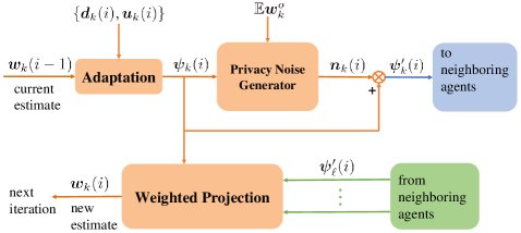
where 𝝈^^n,k2(1)=0subscriptsuperscript^^𝝈2𝑛𝑘10\widehat{\widehat{\bm{\sigma}}}^{2}_{n,k}(-1)=0. A privacy noise 𝒏k(i)subscript𝒏𝑘𝑖{\bm{n}}_{k}(i) is generated at agent k𝑘k by following a distribution with zero mean and variance 𝝈^^n,k2(i)subscriptsuperscript^^𝝈2𝑛𝑘𝑖\widehat{\widehat{\bm{\sigma}}}^{2}_{n,k}(i). This noise is added to the intermediate estimate 𝝍k(i)subscript𝝍𝑘𝑖\bm{\psi}_{k}(i) to form the noisy estimate 𝝍k(i)subscriptsuperscript𝝍𝑘𝑖\bm{\psi}^{\prime}_{k}(i). The quantity 𝝍k(i)subscriptsuperscript𝝍𝑘𝑖\bm{\psi}^{\prime}_{k}(i) is then transmitted to the neighboring agents {𝒩k\{k}}\subscript𝒩𝑘𝑘\left\{\ell\in\mathcal{N}_{k}\backslash\left\{k\right\}\right\}. Fig. 1 summarizes our proposed distributed and adaptive ATP(δ𝛿\delta) algorithm.

Refer to caption
Fig. 1: Diagram of the proposed distributed and adaptive ATP(δ)𝛿(\delta) algorithm.

V Performance Analysis

In this section, we study the mean and mean-square behaviors of the proposed ATP(δ𝛿\delta) algorithm with privacy noise powers {σn,k2(i)=σ^n,k2(i)}superscriptsubscript𝜎𝑛𝑘2𝑖superscriptsubscript^𝜎𝑛𝑘2𝑖\left\{\sigma_{n,k}^{2}(i)=\widehat{\sigma}_{n,k}^{2}(i)\right\}, where the quantities {σ^n,k2(i)}superscriptsubscript^𝜎𝑛𝑘2𝑖\left\{\widehat{\sigma}_{n,k}^{2}(i)\right\} are defined by 54. In addition, we evaluate its privacy-preserving performance.

V-A Mean Behavior Analysis

We have the following theorem for the network mean performance.

Theorem 2.

Consider the distributed strategy 7, 11 and 10 with privacy noise powers {σn,k2(i)=σ^n,k2(i)}superscriptsubscript𝜎𝑛𝑘2𝑖superscriptsubscript^𝜎𝑛𝑘2𝑖\left\{\sigma_{n,k}^{2}(i)=\widehat{\sigma}_{n,k}^{2}(i)\right\}. Suppose that Assumptions 5, 3, 1, 4 and 2 hold, and

11/𝒫(i)1+1/𝒫(i)<λmin(Ru,k)λmax(Ru,k)111delimited-∥∥𝒫𝑖11delimited-∥∥𝒫𝑖subscript𝜆subscript𝑅𝑢𝑘subscript𝜆subscript𝑅𝑢𝑘1\displaystyle\frac{1-1/{\left\lVert{\mathcal{P}(i)}\right\rVert}}{1+1/{\left\lVert{\mathcal{P}(i)}\right\rVert}}<\frac{\lambda_{\min}(R_{u,k})}{\lambda_{\max}(R_{u,k})}\leq 1

for all agents k=1,,N𝑘1𝑁k=1,\ldots,N. If the step-size μksubscript𝜇𝑘\mu_{k} is chosen to satisfy

11/𝒫(i)λmin(Ru,k)<μk<1+1/𝒫(i)λmax(Ru,k)11delimited-∥∥𝒫𝑖subscript𝜆subscript𝑅𝑢𝑘subscript𝜇𝑘11delimited-∥∥𝒫𝑖subscript𝜆subscript𝑅𝑢𝑘\displaystyle\frac{1-1/{\left\lVert{\mathcal{P}(i)}\right\rVert}}{\lambda_{\min}(R_{u,k})}<\mu_{k}<\frac{1+1/{\left\lVert{\mathcal{P}(i)}\right\rVert}}{\lambda_{\max}(R_{u,k})} (64)

for each agent k𝑘k, then

limi𝔼𝒘~(i)=0.subscript𝑖𝔼~𝒘𝑖0\displaystyle\lim_{i\to\infty}\mathbb{E}\widetilde{{\bm{w}}}(i)=0. (65)
Proof.

Let 𝒜(i)𝒫(i)(IMu)𝒜𝑖𝒫𝑖subscript𝐼𝑀subscript𝑢\mathcal{A}(i)\triangleq\mathcal{P}(i)\left(I_{M}-\mathcal{M}\mathcal{R}_{u}\right). Taking expectations on both sides of (LABEL:Eq:Netrror_dynamics) gives

𝔼𝒘~(i)𝔼~𝒘𝑖\displaystyle\mathbb{E}\widetilde{{\bm{w}}}(i) =𝒫(i)𝔼[(IM𝓡u(i))𝒘~(i1)]𝒫(i)𝔼𝒈(i\displaystyle=\mathcal{P}(i)\mathbb{E}\left[{(I_{M}-\mathcal{M}\bm{\mathcal{R}}_{u}(i))\widetilde{{\bm{w}}}(i-1)}\right]-\mathcal{P}(i)\mathcal{M}\mathbb{E}{\bm{g}}(i
𝔼𝒒(i)𝔼𝒒𝑖\displaystyle\hskip 11.38092pt-\mathbb{E}{\bm{q}}(i)
=(a)𝒜(i)𝔼𝒘~(i1)𝒫(i)𝔼𝒈(i)𝔼𝒒(i)superscript(a)absent𝒜𝑖𝔼~𝒘𝑖1𝒫𝑖𝔼𝒈𝑖𝔼𝒒𝑖\displaystyle\stackrel{{\scriptstyle\scriptstyle{\textrm{(a)}}}}{{=}}\mathcal{A}(i)\mathbb{E}\widetilde{{\bm{w}}}(i-1)-\mathcal{P}(i)\mathcal{M}\mathbb{E}{\bm{g}}(i)-\mathbb{E}{\bm{q}}(i)
=(b)𝒜(i)𝔼𝒘~(i1)superscript(b)absent𝒜𝑖𝔼~𝒘𝑖1\displaystyle\stackrel{{\scriptstyle\scriptstyle{\textrm{(b)}}}}{{=}}\mathcal{A}(i)\mathbb{E}\widetilde{{\bm{w}}}(i-1) (66)

where in step (a) we used Assumption 2, and step (b) follows from Assumptions 3, 1 and 4. Using the same proof as in Lemma 2.1 of the supplementary material, ρ(𝒜(i))<1𝜌𝒜𝑖1\rho(\mathcal{A}(i))<1 if 64 holds. The proof is now complete. ∎

V-B Mean-square Performance Analysis

In this subsection, we evaluate the steady-state network MSD, namely, the value of MSDnet(i)subscriptMSDnet𝑖{\mbox{MSD}}_{\mbox{net}}(i) as the time instant i𝑖i\to\infty. Let

(i)=𝔼[((IM𝓡u(i))𝒫(i))((IM𝓡u(i))𝒫(i))],𝑖𝔼delimited-[]tensor-productsubscript𝐼𝑀subscript𝓡𝑢𝑖superscript𝒫𝑖subscript𝐼𝑀subscript𝓡𝑢𝑖superscript𝒫𝑖\mathcal{F}(i)=\mathbb{E}\,\big{[}\left((I_{M}-\bm{\mathcal{R}}_{u}(i)\mathcal{M})\mathcal{P}^{\intercal}(i)\right)\\ \otimes\left((I_{M}-\bm{\mathcal{R}}_{u}(i)\mathcal{M})\mathcal{P}^{\intercal}(i)\right)\big{]}, (69)

where tensor-product\otimes denotes Kronecker product.

Assumption 6.

The noise powers {σn,k2(i)}superscriptsubscript𝜎𝑛𝑘2𝑖\{\sigma_{n,k}^{2}(i)\} converge as i𝑖i\to\infty for all k=1,,N𝑘1𝑁k=1,\ldots,N.

We note that Assumption 6 is satisfied if we set σn,k2(i)=σ^n,k2(i)superscriptsubscript𝜎𝑛𝑘2𝑖superscriptsubscript^𝜎𝑛𝑘2𝑖\sigma_{n,k}^{2}(i)=\widehat{\sigma}_{n,k}^{2}(i) for all agents k=1,,N𝑘1𝑁k=1,\ldots,N and i0𝑖0i\geq 0. Assumption 6 together with the assumption that ωk(i)subscript𝜔𝑘𝑖\omega_{\ell k}(i) defined by 14 converges as i𝑖i\to\infty for any agents ,k=1,,Nformulae-sequence𝑘1𝑁\ell,k=1,\cdots,N lead to the following conclusions:

  1. (a)

    Γ(i)Γ𝑖\Gamma(i) converges as i𝑖i\to\infty.

  2. (b)

    =limi(i)subscript𝑖𝑖\mathcal{F}=\lim_{i\to\infty}\mathcal{F}(i) exists.

In addition, we assume that the quantity (11/𝒫(i))/λmin(Ru,k)11delimited-∥∥𝒫𝑖subscript𝜆subscript𝑅𝑢𝑘\left(1-1/{\left\lVert{\mathcal{P}(i)}\right\rVert}\right)\big{/}{\lambda_{\min}(R_{u,k})} on the LHS of 64 is sufficiently small, so that for sufficiently small step-sizes {μk}subscript𝜇𝑘\left\{\mu_{k}\right\}, we have

=𝒜()𝒜()+O(μmax2)tensor-productsuperscript𝒜superscript𝒜𝑂superscriptsubscript𝜇2\displaystyle\mathcal{F}=\mathcal{A}^{\intercal}(\infty)\otimes\mathcal{A}^{\intercal}(\infty)+O(\mu_{\max}^{2})

where μmaxmax{μ1,,μN}subscript𝜇subscript𝜇1subscript𝜇𝑁\mu_{\max}\triangleq\max\left\{\mu_{1},\ldots,\mu_{N}\right\}. Then if the step-sizes {μk}subscript𝜇𝑘\left\{\mu_{k}\right\} satisfy 64, we have ρ(𝒜())<1𝜌𝒜1\rho\left(\mathcal{A}(\infty)\right)<1, and ρ()(ρ(𝒜()))2<1𝜌superscript𝜌𝒜21\rho\left(\mathcal{F}\right)\thickapprox\left(\rho\left(\mathcal{A}(\infty)\right)\right)^{2}<1, i.e., the matrix \mathcal{F} is stable. Let

σss=1N(IM2)1vec(IM).subscript𝜎ss1𝑁superscriptsubscript𝐼superscript𝑀21vecsubscript𝐼𝑀\displaystyle\sigma_{\textrm{ss}}=\frac{1}{N}\left(I_{M^{2}}-\mathcal{F}\right)^{-1}\operatorname{vec}\left(I_{M}\right). (70)
Theorem 3.

Consider the distributed strategy 7, 11 and 10. Suppose that Assumptions 5, 1, 2, 3, 4 and 6 hold. Then,

MSDnetsubscriptMSDnet\displaystyle{\mbox{MSD}}_{\mbox{net}} limiMSDnet(i)absentsubscript𝑖subscriptMSDnet𝑖\displaystyle\triangleq\lim_{i\to\infty}{\mbox{MSD}}_{\mbox{net}}(i)
=limi[vec(𝒫(i)𝒢𝒫(i))]σssabsentsubscript𝑖superscriptdelimited-[]vec𝒫𝑖𝒢superscript𝒫𝑖subscript𝜎ss\displaystyle=\lim_{i\to\infty}\left[\operatorname{vec}\left(\mathcal{P}(i)\mathcal{M}\mathcal{G}\mathcal{M}\mathcal{P}^{\intercal}(i)\right)\right]^{\intercal}\sigma_{\textrm{ss}}
+limi[vec(Γ(i))]σss.subscript𝑖superscriptdelimited-[]vecΓ𝑖subscript𝜎ss\displaystyle\hskip 11.38092pt+\lim_{i\to\infty}\left[\operatorname{vec}\left(\Gamma(i)\right)\right]^{\intercal}\sigma_{\textrm{ss}}. (71)
Proof.

Note that [46, p.762]

Tr(AB)Tr𝐴𝐵\displaystyle{\operatorname{Tr}\left(AB\right)} =[vec(B)]vec(A)absentsuperscriptdelimited-[]vecsuperscript𝐵vec𝐴\displaystyle=\left[\operatorname{vec}(B^{\intercal})\right]^{\intercal}\operatorname{vec}(A) (72)
vec(ACB)vec𝐴𝐶𝐵\displaystyle\operatorname{vec}(ACB) =(BA)vec(C)absenttensor-productsuperscript𝐵𝐴vec𝐶\displaystyle=(B^{\intercal}\otimes A)\operatorname{vec}(C) (73)

for any matrices {A,B,C}𝐴𝐵𝐶\{A,B,C\} of compatible sizes. Let σ=vec(Σ)𝜎vecΣ\sigma=\operatorname{vec}(\Sigma). Then, it follows from 73 that

σ(i)vec(Σ(i))=(i)σ.superscript𝜎𝑖vecsuperscriptΣ𝑖𝑖𝜎\displaystyle\sigma^{\prime}(i)\triangleq\operatorname{vec}\left(\Sigma^{\prime}(i)\right)=\mathcal{F}(i)\sigma.

Now, we rewrite the recursion Section III-D as

𝔼𝒘~(i)σ2𝔼subscriptsuperscriptdelimited-∥∥~𝒘𝑖2𝜎\displaystyle\mathbb{E}{\left\lVert{\widetilde{{\bm{w}}}(i)}\right\rVert}^{2}_{\sigma} =𝔼𝒘~(i1)(i)σ2+[vec(Γ(i))]σabsent𝔼subscriptsuperscriptdelimited-∥∥~𝒘𝑖12𝑖𝜎superscriptdelimited-[]vecΓ𝑖𝜎\displaystyle=\mathbb{E}{\left\lVert{\widetilde{{\bm{w}}}(i-1)}\right\rVert}^{2}_{\mathcal{F}(i)\sigma}+\left[\operatorname{vec}\left(\Gamma(i)\right)\right]^{\intercal}\sigma
+[vec(𝒫(i)𝒢𝒫(i))]σ,superscriptdelimited-[]vec𝒫𝑖𝒢superscript𝒫𝑖𝜎\displaystyle\hskip 11.38092pt+\left[\operatorname{vec}\left(\mathcal{P}(i)\mathcal{M}\mathcal{G}\mathcal{M}\mathcal{P}^{\intercal}(i)\right)\right]^{\intercal}\sigma, (74)

where we used the property 72. From Assumption 6, we obtain

limi𝔼𝒘~(i)(IM2)σ2subscript𝑖𝔼subscriptsuperscriptdelimited-∥∥~𝒘𝑖2subscript𝐼superscript𝑀2𝜎\displaystyle\lim_{i\to\infty}\mathbb{E}{\left\lVert{\widetilde{{\bm{w}}}(i)}\right\rVert}^{2}_{\left(I_{M^{2}}-\mathcal{F}\right)\sigma} =limi[vec(𝒫(i)𝒢𝒫(i))]σabsentsubscript𝑖superscriptdelimited-[]vec𝒫𝑖𝒢superscript𝒫𝑖𝜎\displaystyle=\lim_{i\to\infty}\left[\operatorname{vec}\left(\mathcal{P}(i)\mathcal{M}\mathcal{G}\mathcal{M}\mathcal{P}^{\intercal}(i)\right)\right]^{\intercal}\sigma
+limi[vec(Γ(i))]σ.subscript𝑖superscriptdelimited-[]vecΓ𝑖𝜎\displaystyle\hskip 11.38092pt+\lim_{i\to\infty}\left[\operatorname{vec}\left(\Gamma(i)\right)\right]^{\intercal}\sigma.

By setting σ=σss𝜎subscript𝜎ss\sigma=\sigma_{\textrm{ss}}, which is defined by 70 on the both sides, we arrive at the desired result Theorem 3 and the proof is complete. ∎

V-C Privacy-preserving Performance

In this subsection, we introduce the performance metrics for inference privacy preservation, and evaluate the privacy-preserving performance of the proposed ATP(δ)𝛿(\delta) algorithm.

Let 𝚽(i)subscript𝚽𝑖\bm{\Phi}_{\ell}(i) be the set of information that an agent \ell has at time instant i0𝑖0i\geq 0 to infer its neighboring agent k𝑘k’s task 𝒘kosuperscriptsubscript𝒘𝑘𝑜{\bm{w}}_{k}^{o}. To quantify the privacy-preserving performance of any scheme, we evaluate, in terms of mean-square error, how well agent \ell can estimate 𝒘kosuperscriptsubscript𝒘𝑘𝑜{\bm{w}}_{k}^{o}. Then we average over the whole network. The network inference privacy error is defined using

ξnet(i)subscript𝜉net𝑖\displaystyle\xi_{\textrm{net}}(i) =1Nk=1N1|𝒩k|1𝒩k\{k}𝔼𝒘ko𝒘^k𝚽(i)2,absent1𝑁superscriptsubscript𝑘1𝑁1subscript𝒩𝑘1subscript\subscript𝒩𝑘𝑘𝔼superscriptdelimited-∥∥superscriptsubscript𝒘𝑘𝑜subscript^𝒘conditional𝑘subscript𝚽𝑖2\displaystyle=\frac{1}{N}\sum_{k=1}^{N}\frac{1}{|\mathcal{N}_{k}|-1}\sum_{\ell\in\mathcal{N}_{k}\backslash\{k\}}\mathbb{E}{\left\lVert{{\bm{w}}_{k}^{o}-\widehat{{\bm{w}}}_{k\mid\bm{\Phi}_{\ell}}(i)}\right\rVert}^{2}, (75)

where 𝒘^k𝚽(i)subscript^𝒘conditional𝑘subscript𝚽𝑖\widehat{{\bm{w}}}_{k\mid\bm{\Phi}_{\ell}}(i) is the least mean-square estimate of 𝒘kosuperscriptsubscript𝒘𝑘𝑜{\bm{w}}_{k}^{o} given 𝚽(i)subscript𝚽𝑖\bm{\Phi}_{\ell}(i). A larger ξnet(i)subscript𝜉net𝑖\xi_{\textrm{net}}(i) implies better average privacy preservation across the network at time instant i𝑖i.

In our numerical experiments, we compare the performance of our proposed ATP(δ)𝛿(\delta) algorithm with the proposed ATP(0) algorithm, the multitask diffusion algorithm [7] (denoted as MDA for convenience) and the non-cooperative LMS algorithm 24 (denoted as NoCoop). Since the unknown coefficient vectors {𝒘ko}superscriptsubscript𝒘𝑘𝑜\left\{{\bm{w}}_{k}^{o}\right\} are linearly related across the network, agent \ell can make use of all neighboring estimates {𝝍s(i)}subscriptsuperscript𝝍𝑠𝑖\left\{\bm{\psi}^{\prime}_{s}(i)\right\} that are available to it at time instant i𝑖i to infer its neighbor’s task 𝒘kosuperscriptsubscript𝒘𝑘𝑜{\bm{w}}_{k}^{o} for any k𝒩𝑘subscript𝒩k\in\mathcal{N}_{\ell}. However, for simplicity, in order to evaluate the privacy-preserving performance of the different schemes, we constrain the information set 𝚽(i)subscript𝚽𝑖\bm{\Phi}_{\ell}(i) as follows:

  • For ATP(δ)𝛿(\delta), we let 𝚽(i)={𝝍(i),𝝍k(i)}subscript𝚽𝑖subscript𝝍𝑖subscriptsuperscript𝝍𝑘𝑖\bm{\Phi}_{\ell}(i)=\{\bm{\psi}_{\ell}(i),\bm{\psi}^{\prime}_{k}(i)\}, i.e., each agent \ell is memoryless across time and spatial domains.

  • For ATP(0)0(0) and MDA, we let 𝚽(i)={𝝍(i),𝝍k(i)}subscript𝚽𝑖subscript𝝍𝑖subscript𝝍𝑘𝑖\bm{\Phi}_{\ell}(i)=\{\bm{\psi}_{\ell}(i),\bm{\psi}_{k}(i)\} since no privacy noises are added in these schemes.

  • For NoCoop, we let 𝚽(i)={𝒘(i)}subscript𝚽𝑖subscript𝒘𝑖\bm{\Phi}_{\ell}(i)=\{{\bm{w}}_{\ell}(i)\} since there is no information exchange between agents.

Let

(76)
(77)

Let 𝝍{k,}(i)=[𝝍k(i),𝝍(i)]subscript𝝍𝑘𝑖superscriptsuperscriptsubscript𝝍𝑘𝑖superscriptsubscript𝝍𝑖\bm{\psi}_{\left\{k,\ell\right\}}(i)=\left[\bm{\psi}_{k}^{\intercal}(i),\bm{\psi}_{\ell}^{\intercal}(i)\right]^{\intercal}. We also define

Uk{k,}(i)=𝔼[(𝒘ko𝔼𝒘ko)(𝝍{k,}(i)𝔼𝝍{k,}(i))]subscript𝑈𝑘𝑘𝑖𝔼delimited-[]superscriptsubscript𝒘𝑘𝑜𝔼superscriptsubscript𝒘𝑘𝑜superscriptsubscript𝝍𝑘𝑖𝔼subscript𝝍𝑘𝑖\displaystyle U_{k\left\{k,\ell\right\}}(i)=\mathbb{E}\left[{\left({\bm{w}}_{k}^{o}-\mathbb{E}{\bm{w}}_{k}^{o}\right)\left(\bm{\psi}_{\left\{k,\ell\right\}}(i)-\mathbb{E}\bm{\psi}_{\left\{k,\ell\right\}}(i)\right)^{\intercal}}\right]
X{k,}{k,}(i)subscript𝑋𝑘𝑘𝑖\displaystyle X_{{\left\{k,\ell\right\}}{\left\{k,\ell\right\}}}(i) =𝔼[(𝝍{k,}(i)𝔼𝝍{k,}(i))\displaystyle=\mathbb{E}\Big{[}\left(\bm{\psi}_{\left\{k,\ell\right\}}(i)-\mathbb{E}\bm{\psi}_{\left\{k,\ell\right\}}(i)\right)
×(𝝍{k,}(i)𝔼𝝍{k,}(i))],\displaystyle\hskip 19.91684pt\times\left(\bm{\psi}_{\left\{k,\ell\right\}}(i)-\mathbb{E}\bm{\psi}_{\left\{k,\ell\right\}}(i)\right)^{\intercal}\Big{]}, (78)

and

Rˇn,k(i)subscriptˇ𝑅𝑛𝑘𝑖\displaystyle\widecheck{R}_{n,k}(i) =[Rn,k(i)000]absentdelimited-[]subscript𝑅𝑛𝑘𝑖000\displaystyle=\left[\begin{array}[]{cc}R_{n,k}(i)&0\\ 0&0\end{array}\right]

where the quantity Rn,k(i)subscript𝑅𝑛𝑘𝑖R_{n,k}(i) is defined by Assumption 4. Let

(i)=𝔼[((IM𝓡u(i+1))𝒫(i))((IM𝓡u(i+1))𝒫(i))],𝑖𝔼delimited-[]tensor-productsubscript𝐼𝑀subscript𝓡𝑢𝑖1𝒫𝑖subscript𝐼𝑀subscript𝓡𝑢𝑖1𝒫𝑖\mathcal{H}(i)=\mathbb{E}\,\big{[}\left(\left(I_{M}-\mathcal{M}\bm{\mathcal{R}}_{u}(i+1)\right)\mathcal{P}(i)\right)\\ \otimes\left(\left(I_{M}-\mathcal{M}\bm{\mathcal{R}}_{u}(i+1)\right)\mathcal{P}(i)\right)\big{]}, (79)
𝒳(i)=𝔼[((IM𝓡u(i+1))f(i))((IM𝓡u(i+1))𝒫(i))],𝒳𝑖𝔼delimited-[]tensor-productsubscript𝐼𝑀subscript𝓡𝑢𝑖1𝑓𝑖subscript𝐼𝑀subscript𝓡𝑢𝑖1𝒫𝑖\mathcal{X}(i)=\mathbb{E}\,\big{[}\left(\left(I_{M}-\mathcal{M}\bm{\mathcal{R}}_{u}(i+1)\right)f(i)\right)\\ \otimes\left(\left(I_{M}-\mathcal{M}\bm{\mathcal{R}}_{u}(i+1)\right)\mathcal{P}(i)\right)\big{]}, (80)
𝒳(i)=𝔼[((IM𝓡u(i+1))𝒫(i))((IM𝓡u(i+1))f(i))],superscript𝒳𝑖𝔼delimited-[]tensor-productsubscript𝐼𝑀subscript𝓡𝑢𝑖1𝒫𝑖subscript𝐼𝑀subscript𝓡𝑢𝑖1𝑓𝑖\mathcal{X}^{\prime}(i)=\mathbb{E}\,\big{[}\left(\left(I_{M}-\mathcal{M}\bm{\mathcal{R}}_{u}(i+1)\right)\mathcal{P}(i)\right)\\ \otimes\left(\left(I_{M}-\mathcal{M}\bm{\mathcal{R}}_{u}(i+1)\right)f(i)\right)\big{]}, (81)

and

(82)

all of which except C4subscript𝐶4C_{4} depend on the quantities {𝒫(i),f(i)}𝒫𝑖𝑓𝑖\{\mathcal{P}(i),f(i)\} at time instant i𝑖i. We also define In the following Theorem 4, we evaluate the privacy-preserving performance of the proposed ATP(δ𝛿\delta) algorithm.

Theorem 4.

Consider the distributed strategy 7, 11 and 10. Suppose that Assumptions 1, 2, 3 and 4 hold. The network inference error at each time instant i0𝑖0i\geq 0 is

ξnetATP(δ)(i)=1Nk=1N1|𝒩k|1𝒩k\{k}Tr(WkkUk{k,}(i)(X{k,}{k,}(i)+Rˇn,k(i))1Uk{k,}(i))superscriptsubscript𝜉netATP(δ)𝑖1𝑁superscriptsubscript𝑘1𝑁1subscript𝒩𝑘1subscript\subscript𝒩𝑘𝑘Trsubscript𝑊𝑘𝑘subscript𝑈𝑘𝑘𝑖superscriptsubscript𝑋𝑘𝑘𝑖subscriptˇ𝑅𝑛𝑘𝑖1superscriptsubscript𝑈𝑘𝑘𝑖\xi_{\textrm{net}}^{\textrm{ATP($\delta$)}}(i)=\frac{1}{N}\sum_{k=1}^{N}\frac{1}{|\mathcal{N}_{k}|-1}\sum_{\ell\in\mathcal{N}_{k}\backslash\{k\}}\operatorname{Tr}\bigg{(}W_{kk}\\ -U_{k\left\{k,\ell\right\}}(i)\left(X_{{\left\{k,\ell\right\}}{\left\{k,\ell\right\}}}(i)+\widecheck{R}_{n,k}(i)\right)^{-1}U_{k\left\{k,\ell\right\}}^{\intercal}(i)\bigg{)} (85)

where

Uk{k,}(i)subscript𝑈𝑘𝑘𝑖\displaystyle U_{k\left\{k,\ell\right\}}(i) =[[𝒲𝒱(i)]k,k,[𝒲𝒱(i)]k,],absentsubscriptdelimited-[]𝒲𝒱𝑖𝑘𝑘subscriptdelimited-[]𝒲𝒱𝑖𝑘\displaystyle=\left[\left[\mathcal{W}-\mathcal{V}(i)\right]_{k,k},\left[\mathcal{W}-\mathcal{V}(i)\right]_{k,\ell}\right], (86)
𝒱(i+1)𝒱𝑖1\displaystyle\mathcal{V}(i+1) =𝒱(i)(i),absent𝒱𝑖superscript𝑖\displaystyle=\mathcal{V}(i)\mathcal{B}^{\intercal}(i), (87)
𝒱(0)𝒱0\displaystyle\mathcal{V}(0) =𝒲(IMu),absent𝒲subscript𝐼𝑀subscript𝑢\displaystyle=\mathcal{W}\,(I_{M}-\mathcal{M}\mathcal{R}_{u}), (88)

and where

X{k,}{k,}(i)=[[Ψ(i)𝔼𝝍(i)(𝔼𝝍(i))]k,k[Ψ(i)𝔼𝝍(i)(𝔼𝝍(i))]k,[Ψ(i)𝔼𝝍(i)(𝔼𝝍(i))],k[Ψ(i)𝔼𝝍(i)(𝔼𝝍(i))],]subscript𝑋𝑘𝑘𝑖delimited-[]subscriptdelimited-[]Ψ𝑖𝔼𝝍𝑖superscript𝔼𝝍𝑖𝑘𝑘subscriptdelimited-[]Ψ𝑖𝔼𝝍𝑖superscript𝔼𝝍𝑖𝑘subscriptdelimited-[]Ψ𝑖𝔼𝝍𝑖superscript𝔼𝝍𝑖𝑘subscriptdelimited-[]Ψ𝑖𝔼𝝍𝑖superscript𝔼𝝍𝑖X_{{\left\{k,\ell\right\}}{\left\{k,\ell\right\}}}(i)=\left[\!\!\begin{array}[]{cc}\left[\Psi(i)\!-\!\mathbb{E}\bm{\psi}(i)\left(\mathbb{E}\bm{\psi}(i)\right)^{\intercal}\right]_{k,k}&\!\left[\Psi(i)\!-\!\mathbb{E}\bm{\psi}(i)\left(\mathbb{E}\bm{\psi}(i)\right)^{\intercal}\right]_{k,\ell}\\ \left[\Psi(i)\!-\!\mathbb{E}\bm{\psi}(i)\left(\mathbb{E}\bm{\psi}(i)\right)^{\intercal}\right]_{\ell,k}&\!\left[\Psi(i)\!-\!\mathbb{E}\bm{\psi}(i)\left(\mathbb{E}\bm{\psi}(i)\right)^{\intercal}\right]_{\ell,\ell}\end{array}\!\!\right] (91)

with

𝔼𝝍(0)𝔼𝝍0\displaystyle\mathbb{E}\bm{\psi}(0) =u𝔼𝒘o,absentsubscript𝑢𝔼superscript𝒘𝑜\displaystyle=\mathcal{M}\mathcal{R}_{u}\mathbb{E}{\bm{w}}^{o}, (92)
𝔼𝝍(i+1)𝔼𝝍𝑖1\displaystyle\mathbb{E}\bm{\psi}(i+1) =(IMu)𝒫(i)𝔼𝝍(i)absentsubscript𝐼𝑀subscript𝑢𝒫𝑖𝔼𝝍𝑖\displaystyle=\left(I_{M}-\mathcal{M}\mathcal{R}_{u}\right)\mathcal{P}(i)\mathbb{E}\bm{\psi}(i)
(IMu)f(i)+u𝔼𝒘o,subscript𝐼𝑀subscript𝑢𝑓𝑖subscript𝑢𝔼superscript𝒘𝑜\displaystyle\hskip 11.38092pt-\left(I_{M}-\mathcal{M}\mathcal{R}_{u}\right)f(i)+\mathcal{M}\mathcal{R}_{u}\mathbb{E}{\bm{w}}^{o}, (93)

and

vec(Ψ(i+1))=(i)vec(Ψ(i))+𝒵vec(Γ(i))+c(i)vecΨ𝑖1𝑖vecΨ𝑖𝒵vecΓ𝑖𝑐𝑖\displaystyle\operatorname{vec}\left(\Psi(i+1)\right)=\mathcal{H}(i)\operatorname{vec}\left(\Psi(i)\right)+\mathcal{Z}\operatorname{vec}(\Gamma(i))+c(i)
+(𝒴(i)𝒳(i)𝒳(i)+𝒴(i))𝔼𝝍(i).𝒴𝑖𝒳𝑖superscript𝒳𝑖superscript𝒴𝑖𝔼𝝍𝑖\displaystyle\hskip 72.55461pt+\left(\mathcal{Y}(i)-\mathcal{X}(i)-\mathcal{X}^{\prime}(i)+\mathcal{Y}^{\prime}(i)\right)\,\mathbb{E}\bm{\psi}(i). (94)
Proof.

See Section 3 of the supplementary material. ∎

VI Simulation Results

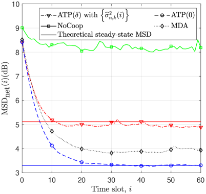
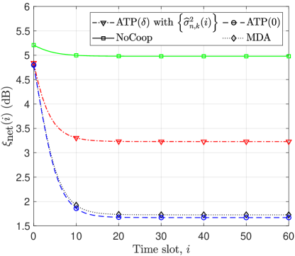
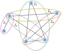
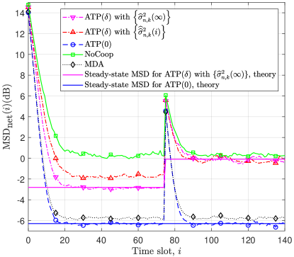
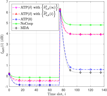
In this section, we compare performance of the proposed ATP(δ)𝛿(\delta) algorithm in terms of network inference privacy and network MSD against ATP(0)0(0), MDA [7] and NoCoop 24 in two types of networks: 1) a line network with a large number of linear equality constraints; and 2) a very dense network with a small number of linear equality constraints. We also test the tracking performance of the proposed distributed and adaptive ATP(δ)𝛿(\delta) algorithm in the case of changing statistics.

VI-A Selection of Weights for Weighted Projection

Note that the projection step 11 at each agent k𝑘k involves noisy intermediate estimates {𝝍(i)}subscriptsuperscript𝝍𝑖\{\bm{\psi}^{\prime}_{\ell}(i)\} from its neighbors {𝒩k\{k}}\subscript𝒩𝑘𝑘\{\ell\in\mathcal{N}_{k}\backslash\{k\}\} and the uncontaminated intermediate estimate 𝝍k(i)subscript𝝍𝑘𝑖\bm{\psi}_{k}(i). In view of the fact that the noisy intermediate estimate 𝝍(i)subscriptsuperscript𝝍𝑖\bm{\psi}^{\prime}_{\ell}(i) involves a privacy noise 𝒏(i)subscript𝒏𝑖{\bm{n}}_{\ell}(i) with variance σn,2(i)superscriptsubscript𝜎𝑛2𝑖\sigma_{n,\ell}^{2}(i), we set the weights {ωk(i)}subscript𝜔𝑘𝑖\left\{\omega_{\ell k}(i)\right\} defined by 13 to

ωk(i)={eσn,2(i)𝒩k\{k}eσn,2(i)+1,if 𝒩k\{k}1𝒩k\{k}eσn,2(i)+1,if =ksubscript𝜔𝑘𝑖casessuperscript𝑒superscriptsubscript𝜎𝑛2𝑖subscript\subscript𝒩𝑘𝑘superscript𝑒superscriptsubscript𝜎𝑛2𝑖1if 𝒩k\{k}1subscript\subscript𝒩𝑘𝑘superscript𝑒superscriptsubscript𝜎𝑛2𝑖1if =k\displaystyle\omega_{\ell k}(i)=\left\{\begin{array}[]{ll}\frac{e^{-\sigma_{n,\ell}^{2}(i)}}{\sum_{\ell\in\mathcal{N}_{k}\backslash\{k\}}e^{-\sigma_{n,\ell}^{2}(i)}+1},&\text{if $\ell\in\mathcal{N}_{k}\backslash\{k\}$}\\ \frac{1}{\sum_{\ell\in\mathcal{N}_{k}\backslash\{k\}}e^{-\sigma_{n,\ell}^{2}(i)}+1},&\text{if $\ell=k$}\end{array}\right. (97)

which satisfies the requirements in 14.

VI-B Line Network

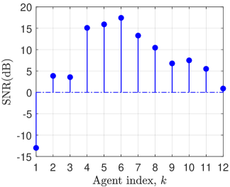
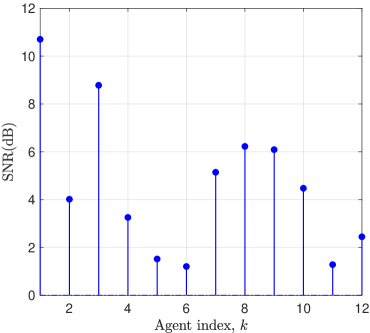
As shown in Fig. 2(a), we consider a line network which consists of N=12𝑁12N=12 agents. The agents in the network are involved in Q=11𝑄11Q=11 linear equality constraints. Let qsubscript𝑞\mathcal{I}_{q} be the set of agents involved in the q𝑞q-th constraint for any q=1,,Q𝑞1𝑄q=1,\ldots,Q. Then in the case of a line network, each qsubscript𝑞\mathcal{I}_{q} only contains two neighboring agents that are connected by an edge. Each linear equality constraint is of the form [7]:

kqdqk𝒘ko+bq𝟏3×1=03×1,q=1,,Qformulae-sequencesubscript𝑘subscript𝑞subscript𝑑𝑞𝑘superscriptsubscript𝒘𝑘𝑜subscript𝑏𝑞subscript131subscript031𝑞1𝑄\displaystyle\sum_{k\in\mathcal{I}_{q}}d_{qk}{\bm{w}}_{k}^{o}+b_{q}\mathbf{1}_{3\times 1}=0_{3\times 1},\quad q=1,\ldots,Q (98)

with the scalar parameters {dqk,bq}subscript𝑑𝑞𝑘subscript𝑏𝑞\{d_{qk},b_{q}\} randomly selected from [3,1][1,3]3113[-3,-1]\cup[1,3]. The lengths of the unknown parameter vectors {𝒘ko}superscriptsubscript𝒘𝑘𝑜\{{\bm{w}}_{k}^{o}\} are {Mk3}subscript𝑀𝑘3\{M_{k}\equiv 3\}. The random data {𝒖k(i),𝒗k(i)}subscript𝒖𝑘𝑖subscript𝒗𝑘𝑖\{{\bm{u}}_{k}(i),{\bm{v}}_{k}(i)\} are independent, normally distributed with zero mean, and white over time and space. Let

SNRk=10log10(𝔼[(𝒖k(i)𝒘ko)2]/σv,k2\displaystyle\mbox{SNR}_{k}=10\log_{10}\left(\mathbb{E}\left[{({\bm{u}}_{k}^{\intercal}(i){\bm{w}}_{k}^{o})^{2}}\right]/\sigma_{v,k}^{2}

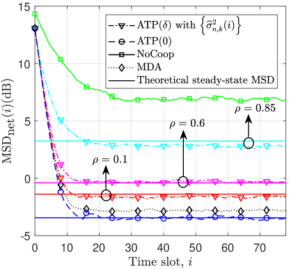
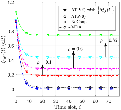
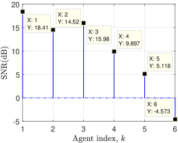
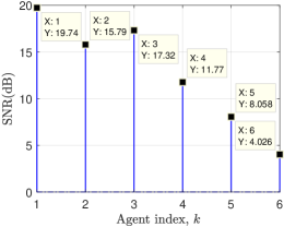
be the signal-to-noise ratio (SNR) at agent k𝑘k. Then, the parameters {Ru,k,Wkk,𝔼𝒘ko,σv,k2}subscript𝑅𝑢𝑘subscript𝑊𝑘𝑘𝔼superscriptsubscript𝒘𝑘𝑜superscriptsubscript𝜎𝑣𝑘2\{R_{u,k},W_{kk},\mathbb{E}{\bm{w}}_{k}^{o},\sigma_{v,k}^{2}\} are adjusted to make {SNRk}subscriptSNR𝑘\{\mbox{SNR}_{k}\} as shown in Fig. 2(b). For the step-size parameters, we set {μk0.02}subscript𝜇𝑘0.02\{\mu_{k}\equiv 0.02\} for all the tested algorithms except MDA, where we set {μk/jk0.02}subscript𝜇𝑘subscript𝑗𝑘0.02\{\mu_{k}/j_{k}\equiv 0.02\} to ensure the same step-size in the adaptation step for all the above-mentioned algorithms. Let δkρTr(Wkk)subscript𝛿𝑘𝜌Trsubscript𝑊𝑘𝑘\delta_{k}\triangleq\rho\,{\operatorname{Tr}\left(W_{kk}\right)} with 0ρ10𝜌10\leq\rho\leq 1. Then, for the ATP(δ)𝛿(\delta) algorithm, we set ρ=0.1,ρ=0.6,ρ=0.85formulae-sequence𝜌0.1formulae-sequence𝜌0.6𝜌0.85\rho=0.1,\,\rho=0.6,\,\rho=0.85, respectively, to compare performance under different privacy thresholds {δk}subscript𝛿𝑘\left\{\delta_{k}\right\}.

Fig. 3 shows the network MSD learning curves of the tested strategies, which are averaged over 1,000 independent realizations of {𝒘ko}superscriptsubscript𝒘𝑘𝑜\{{\bm{w}}_{k}^{o}\}. We observe that 1) simulation results match well with theoretical findings, 2) by adding privacy noises, the proposed ATP(δ)𝛿(\delta) algorithm converges to a higher MSD level than ATP(0) and MDA [7], 3) larger privacy thresholds result in a higher steady-state network MSD. Fig. 4 plots the network inference error, defined by 75. We observe that 1) the network inference privacy performance of ATP(0) and MDA [7] are similar, but worse (lower values of {ξnet(i)}subscript𝜉net𝑖\{\xi_{\textrm{net}}(i)\}) than the proposed ATP(δ)𝛿(\delta), 2) by increasing privacy thresholds, the proposed ATP(δ)𝛿(\delta) algorithm shows better network inference privacy performance. These results demonstrate that the proposed ATP(δ)𝛿(\delta) algorithm is able to balance the trade-off between network MSD and privacy protection.
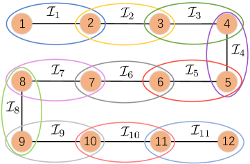
Refer to caption
(a)
Refer to caption
(b)
Fig. 2: (a) A line network and (b) SNRs across the agents in a line network.
Refer to caption
Fig. 3: Network MSD learning curves of MDA [7], NoCoop, the proposed ATP(δ)𝛿(\delta) under different parameter settings for {δk}subscript𝛿𝑘\left\{\delta_{k}\right\}, and ATP(0) in a line network.
Refer to caption
Fig. 4: Network inference privacy learning curves of MDA [7], NoCoop, the proposed ATP(δ)𝛿(\delta) under different parameter settings for {δk}subscript𝛿𝑘\left\{\delta_{k}\right\}, and ATP(0) in a line network.

VI-C Dense Network

As shown in Fig. 5(a), we consider a dense network which consists of N=12𝑁12N=12 agents. The agents in the network are involved in Q=4𝑄4Q=4 linear equality constraints, each of the form 98. The lengths of the unknown parameter vectors {𝒘ko}superscriptsubscript𝒘𝑘𝑜\{{\bm{w}}_{k}^{o}\} are {Mk3}subscript𝑀𝑘3\{M_{k}\equiv 3\}. The random data {𝒖k(i),𝒗k(i)}subscript𝒖𝑘𝑖subscript𝒗𝑘𝑖\{{\bm{u}}_{k}(i),{\bm{v}}_{k}(i)\} are independent, normally distributed with zero mean, and white over time and space. The parameters {Ru,k,Wkk,𝔼𝒘ko,σv,k2}subscript𝑅𝑢𝑘subscript𝑊𝑘𝑘𝔼superscriptsubscript𝒘𝑘𝑜superscriptsubscript𝜎𝑣𝑘2\{R_{u,k},W_{kk},\mathbb{E}{\bm{w}}_{k}^{o},\sigma_{v,k}^{2}\} are adjusted to make {SNRk}subscriptSNR𝑘\{\mbox{SNR}_{k}\} as shown in Fig. 5(b). For the ATP(δ)𝛿(\delta) algorithm, we set the threshold values {δk=0.1Tr(Wkk)}k=1Nsuperscriptsubscriptsubscript𝛿𝑘0.1Trsubscript𝑊𝑘𝑘𝑘1𝑁\{\delta_{k}=0.1\,{\operatorname{Tr}\left(W_{kk}\right)}\}_{k=1}^{N}. The other parameter settings remain the same as those in the previous simulation.

Fig. 6 shows the network MSD learning curves of the tested strategies, which are averaged over 20,000 independent realizations of {𝒘ko}superscriptsubscript𝒘𝑘𝑜\{{\bm{w}}_{k}^{o}\}. Fig. 7 plots the network inference error, defined by 75. These results demonstrate that the proposed ATP(δ)𝛿(\delta) algorithm is still able to balance the trade-off between network MSD and privacy protection in dense networks. Table I lists the ratios of privacy gain to accuracy loss in the line and dense network, where the privacy gain is the absolute gap between the steady-state network inference privacy errors of ATP(0) and ATP(δ)𝛿(\delta) in dB, and the accuracy loss is the absolute gap between the steady-state network MSDs in dB. We observe that the ratio in the dense network is much higher than in the line network, which means that more privacy gains are obtained in the former case with the same quantity of network MSD loss. These results demonstrate that the proposed ATP(δ)𝛿(\delta) algorithm performs better in dense networks than in line networks.
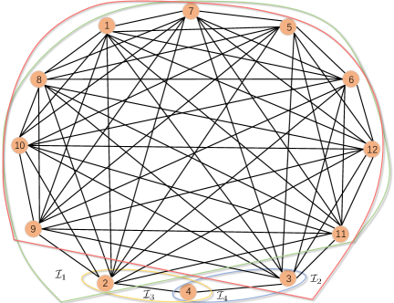
Refer to caption
(a)
Refer to caption
(b)
Fig. 5: (a) A dense network and (b) SNRs across the agents in a dense network.
Refer to caption
Fig. 6: Network MSD learning curves of MDA [7], NoCoop, the proposed ATP(δ)𝛿(\delta) and ATP(0) in a dense network.
Refer to caption
Fig. 7: Network inference privacy learning curves of MDA [7], NoCoop, the proposed ATP(δ)𝛿(\delta) and ATP(0) in a dense network.
TABLE I: Ratio of Privacy Gain to Accuracy Loss
Line Network Dense Network
ρ=0.1𝜌0.1\rho=0.1 ρ=0.6𝜌0.6\rho=0.6 ρ=0.85𝜌0.85\rho=0.85
0.09 0.09 0.06 0.86

VI-D Tracking Performance

As shown in Fig. 8(a), we consider the case where there are N=6𝑁6N=6 agents in the network. The agents in the network are involved in Q=5𝑄5Q=5 linear equality constraints, each of the form [7]:

kqdqk𝒘ko+bq𝟏2×1=02×1,q=1,,Qformulae-sequencesubscript𝑘subscript𝑞subscript𝑑𝑞𝑘superscriptsubscript𝒘𝑘𝑜subscript𝑏𝑞subscript121subscript021𝑞1𝑄\displaystyle\sum_{k\in\mathcal{I}_{q}}d_{qk}{\bm{w}}_{k}^{o}+b_{q}\mathbf{1}_{2\times 1}=0_{2\times 1},\quad q=1,\ldots,Q

with the scalar parameters {dqk,bq}subscript𝑑𝑞𝑘subscript𝑏𝑞\{d_{qk},b_{q}\} randomly selected from [3,1][1,3]3113[-3,-1]\cup[1,3]. The lengths of the unknown parameter vectors {𝒘ko}superscriptsubscript𝒘𝑘𝑜\{{\bm{w}}_{k}^{o}\} are {Mk2}subscript𝑀𝑘2\{M_{k}\equiv 2\}. The random data {𝒖k(i),𝒗k(i)}subscript𝒖𝑘𝑖subscript𝒗𝑘𝑖\{{\bm{u}}_{k}(i),{\bm{v}}_{k}(i)\} are independent, normally distributed with zero mean, and white over time and space. The parameters {Ru,k,Wkk,𝔼𝒘ko,σv,k2}subscript𝑅𝑢𝑘subscript𝑊𝑘𝑘𝔼superscriptsubscript𝒘𝑘𝑜superscriptsubscript𝜎𝑣𝑘2\{R_{u,k},W_{kk},\mathbb{E}{\bm{w}}_{k}^{o},\sigma_{v,k}^{2}\} are adjusted to make {SNRk}subscriptSNR𝑘\{\mbox{SNR}_{k}\} as shown in Fig. 8(b) at the first stage. Then in order to test the tracking performance of the proposed distributed and adaptive ATP(δ𝛿\delta) algorithm, we increase values of the elements in Wkksubscript𝑊𝑘𝑘W_{kk} at time instant i=75𝑖75i=75, which makes {SNRk}subscriptSNR𝑘\{\mbox{SNR}_{k}\} as shown in Fig. 8(c) at the second stage. For the step-size parameters, we set {μk0.02}subscript𝜇𝑘0.02\{\mu_{k}\equiv 0.02\} for all the tested algorithms except MDA, where we set {μk/jk0.02}subscript𝜇𝑘subscript𝑗𝑘0.02\{\mu_{k}/j_{k}\equiv 0.02\} to ensure the same step-size in the adaptation step for all the above-mentioned algorithms. In addition, for the ATP(δ)𝛿(\delta) algorithm, we set the threshold values {δk=0.6Tr(Wkk)}k=1Nsuperscriptsubscriptsubscript𝛿𝑘0.6Trsubscript𝑊𝑘𝑘𝑘1𝑁\{\delta_{k}=0.6\,{\operatorname{Tr}\left(W_{kk}\right)}\}_{k=1}^{N} according to the covariance matrix Wkksubscript𝑊𝑘𝑘W_{kk} at the first stage.

Fig. 9 shows the network MSD learning curves of the tested strategies, which are averaged over 1,000 independent runs. We observe that by increasing values of the elements in Wkksubscript𝑊𝑘𝑘W_{kk}, the proposed ATP(δ)𝛿(\delta) algorithm with privacy noise powers {σn,k2(i)=σ^n,k2()}superscriptsubscript𝜎𝑛𝑘2𝑖superscriptsubscript^𝜎𝑛𝑘2\left\{\sigma_{n,k}^{2}(i)=\widehat{\sigma}_{n,k}^{2}(\infty)\right\} converges to a higher MSD level at the second stage. This is because privacy noise powers become larger at the second stage according to 59. We also note that the steady-state network MSD of the proposed distributed and adaptive ATP(δ)𝛿(\delta) gets higher at the second stage. Fig. 10 plots the network inference error, defined by 75. We observe that the network inference privacy performance of both ATP(δ)𝛿(\delta) algorithms are similar throughout the whole process. These results demonstrate that the proposed distributed and adaptive ATP(δ)𝛿(\delta) algorithm is able to track changes of the covariance matrix Wkksubscript𝑊𝑘𝑘W_{kk}.

Refer to caption
(a)
Refer to caption
(b)
Refer to caption
(c)
Fig. 8: (a) Network topology, (b) SNRs across the agents at the first stage and (c) SNRs across the agents at the second stage.
Refer to caption
Fig. 9: Network MSD learning curves of MDA [7], NoCoop, the proposed ATP(δ)𝛿(\delta) with privacy noise powers {σ^n,k2()}superscriptsubscript^𝜎𝑛𝑘2\left\{\widehat{\sigma}_{n,k}^{2}(\infty)\right\} as shown by 59 and {σ^^n,k2(i)}superscriptsubscript^^𝜎𝑛𝑘2𝑖\left\{\widehat{\widehat{\sigma}}_{n,k}^{2}(i)\right\} as shown by 63, and ATP(0).
Refer to caption
Fig. 10: Network inference privacy learning curves of MDA [7], NoCoop, the proposed ATP(δ)𝛿(\delta) with privacy noise powers {σ^n,k2()}superscriptsubscript^𝜎𝑛𝑘2\left\{\widehat{\sigma}_{n,k}^{2}(\infty)\right\} as shown by 59 and {σ^^n,k2(i)}superscriptsubscript^^𝜎𝑛𝑘2𝑖\left\{\widehat{\widehat{\sigma}}_{n,k}^{2}(i)\right\} as shown by 63, and ATP(0).

VII Conclusion

We have developed a privacy-preserving distributed strategy over linear multitask networks, which is able to protect each agent’s local task by adding a privacy noise to its local information before sharing with its neighbors. We proposed a utility-privacy optimization trade-off to determine the amount of noise to add, and derived a sufficient condition for the privacy noise powers in order to satisfy the proposed privacy constraints. Furthermore, we proposed a distributed and adaptive scheme to compute the privacy noise powers. We have studied the mean and mean-square behaviors and privacy-preserving performance. Simulation results demonstrated that the proposed scheme is able to balance the trade-off between the network MSD and network inference privacy.

Future work concerns privacy issues over multitask networks where agents’ local parameters of interest consist of common parameters within each neighborhood and individual parameters. Privacy-preserving distributed strategies will be developed to improve the estimation accuracy of common parameters at each agent via in-network cooperation with neighboring agents, as well as to protect individual parameters against privacy leakage.

References

  • [1] J. Chen, C. Richard, and A. H. Sayed, “Multitask diffusion adaptation over networks,” IEEE Trans. Signal Process., vol. 62, no. 16, pp. 4129 – 4144, Aug. 2014.
  • [2] ——, “Diffusion LMS over multitask networks,” IEEE Trans. Signal Process., vol. 63, no. 11, pp. 2733 – 2748, Jun. 2015.
  • [3] M. Leng, W. P. Tay, T. Q. S. Quek, and H. Shin, “Distributed local linear parameter estimation using Gaussian SPAWN,” IEEE Trans. Signal Process., vol. 63, no. 1, pp. 244 – 257, Jan. 2015.
  • [4] J. Plata-Chaves, N. Bogdanović, and K. Berberidis, “Distributed diffusion-based LMS for node-specific adaptive parameter estimation,” IEEE Trans. Signal Process., vol. 63, no. 13, pp. 3448 – 3460, Jul. 2015.
  • [5] R. Nassif, C. Richard, A. Ferrari, and A. H. Sayed, “Proximal multitask learning over networks with sparsity-inducing coregularization,” IEEE Trans. Signal Process., vol. 64, no. 23, pp. 6329 – 6344, Dec. 2016.
  • [6] J. Chen, C. Richard, and A. H. Sayed, “Multitask diffusion adaptation over networks with common latent representations,” IEEE J. Sel. Topics Signal Process., vol. 11, no. 3, pp. 563 – 579, Apr. 2017.
  • [7] R. Nassif, C. Richard, A. Ferrari, and A. H. Sayed, “Diffusion LMS for multitask problems with local linear equality constraints,” IEEE Trans. Signal Process., vol. 65, no. 19, pp. 4979 – 4993, Oct. 2017.
  • [8] Y. Wang, W. P. Tay, and W. Hu, “A multitask diffusion strategy with optimized inter-cluster cooperation,” IEEE J. Sel. Topics Signal Process., vol. 11, no. 3, pp. 504 – 517, Apr. 2017.
  • [9] M. Chan, E. Campo, D. Estève, and J.-Y. Fourniols, “Smart homes – Current features and future perspectives,” Maturitas, vol. 64, no. 2, pp. 90 – 97, Oct. 2009.
  • [10] A. Whitmore, A. Agarwal, and L. Da Xu, “The Internet of Things – A survey of topics and trends,” Information Systems Frontiers, vol. 17, no. 2, pp. 261 – 274, Apr. 2015.
  • [11] S. H. Shah and I. Yaqoob, “A survey: Internet of Things (IoT) technologies, applications and challenges,” in Proc. IEEE Smart Energy Grid Engineering, Oshawa, ON, Canada, Aug. 2016.
  • [12] S. Li, L. Da Xu, and S. Zhao, “5G Internet of Things: A survey,” J. of Ind. Inf. Integration, vol. 10, pp. 1 – 9, Jun. 2018.
  • [13] W. Hu and W. P. Tay, “Multi-hop diffusion LMS for energy-constrained distributed estimation,” IEEE Trans. Signal Process., vol. 63, no. 15, pp. 4022 – 4036, Aug. 2015.
  • [14] W. P. Tay, J. N. Tsitsiklis, and M. Z. Win, “Data fusion trees for detection: Does architecture matter?” IEEE Trans. Inf. Theory, vol. 54, no. 9, pp. 4155 – 4168, Sep. 2008.
  • [15] W. P. Tay, “Whose opinion to follow in multihypothesis social learning? A large deviations perspective,” IEEE J. Sel. Topics Signal Process., vol. 9, no. 2, pp. 344 – 359, Mar. 2015.
  • [16] J. Ho, W. P. Tay, T. Q. Quek, and E. K. Chong, “Robust decentralized detection and social learning in tandem networks,” IEEE Trans. Signal Process., vol. 63, no. 19, pp. 5019 – 5032, Oct. 2015.
  • [17] Y. Wang, X. Wu, and H. Donghui, “Using randomized response for differential privacy preserving data collection,” in Proc. ACM SIGKDD Int. Conf. on Knowledge Discovery and Data Mining, Washington, D.C., USA, Aug. 2003.
  • [18] S. Xiong, A. D. Sarwate, and N. B. Mandayam, “Randomized requantization with local differential privacy,” in Proc. IEEE Int. Conf. Acoustics, Speech, and Signal Processing, Shanghai, China, Mar. 2016.
  • [19] A. D. Sarwate and L. Sankar, “A rate-disortion perspective on local differential privacy,” in Proc. Allerton Conf. on Commun., Control and Computing, Monticello, IL, USA, Sep. 2014.
  • [20] J. Liao, L. Sankar, F. P. Calmon, and V. Y. Tan, “Hypothesis testing under maximal leakage privacy constraints,” in Proc. IEEE Int. Symp. on Inform. Theory, Aachen, Germany, Jun. 2017.
  • [21] H. Imtiaz and A. D. Sarwate, “Differentially private distributed principal component analysis,” in Proc. IEEE Int. Conf. Acoustics, Speech, and Signal Processing, Calgary, Alberta, Canada, Apr. 2018.
  • [22] X. Ren, C.-M. Yu, W. Yu, S. Yang, X. Yang, J. A. McCann, and S. Y. Philip, “LoPub: High-dimensional crowdsourced data publication with local differential privacy,” IEEE Trans. Inf. Forensics Security, vol. 13, no. 9, pp. 2151 – 2166, Mar. 2018.
  • [23] B. Razeghi and S. Voloshynovskiy, “Privacy-preserving outsourced media search using secure sparse ternary codes,” in Proc. IEEE Int. Conf. Acoustics, Speech, and Signal Processing, Calgary, Alberta, Canada, Apr. 2018.
  • [24] F. D. McSherry, “Privacy integrated queries: An extensible platform for privacy-preserving data analysis,” in Proc. ACM SIGMOD Inter. Conf. Management of data, Providence, Rhode Island, USA, Jun. 2009.
  • [25] C. Dwork, K. Kenthapadi, F. McSherry, I. Mironov, and M. Naor, “Our data, ourselves: Privacy via distributed noise generation,” in Annual Inter. Conf. on the Theory and Applications of Cryptographic Techniques, St. Petersburg, Russia, May 2006.
  • [26] J. C. Duchi, M. I. Jordan, and M. J. Wainwright, “Local privacy and statistical minimax rates,” in Proc. IEEE Symp. on Foundations of Computer Science, Monticello, IL, USA, Oct. 2013.
  • [27] Y. Mo and R. M. Murray, “Privacy preserving average consensus,” IEEE Trans. Autom. Control, vol. 62, no. 2, pp. 753 – 765, Feb. 2017.
  • [28] E. Nozari, P. Tallapragada, and J. Cortés, “Differentially private average consensus: Obstructions, trade-offs, and optimal algorithm design,” Automatica, vol. 81, pp. 221 – 231, 2017.
  • [29] J. He, L. Cai, and X. Guan, “Preserving data-privacy with added noises: Optimal estimation and privacy analysis,” IEEE Trans. Inf. Theory, vol. 64, no. 8, pp. 5677 – 5690, Aug. 2018.
  • [30] J. He, L. Cai, C. Zhao, P. Cheng, and X. Guan, “Privacy-preserving average consensus: Privacy analysis and algorithm design,” IEEE Trans. Signal Inf. Process. Netw., vol. 5, no. 1, pp. 127– 138, Mar. 2019.
  • [31] X. Wang, J. He, P. Cheng, and J. Chen, “Privacy preserving collaborative computing: Heterogeneous privacy guarantee and efficient incentive mechanism,” IEEE Trans. Signal Process., vol. 67, no. 1, pp. 221 – 233, Jan. 2019.
  • [32] M. Sun, W. P. Tay, and X. He, “Toward information privacy for the Internet of Things: A non-parametric learning approach,” IEEE Trans. Signal Process., vol. 66, no. 7, pp. 1734 – 1747, Apr. 2018.
  • [33] X. He, W. P. Tay, H. Lei, M. Sun, and Y. Gong, “Privacy-aware sensor network via multilayer nonlinear processing,” IEEE Internet Things J., vol. 6, no. 6, pp. 10 834 – 10 845, Dec. 2019.
  • [34] M. Sun and W. P. Tay, “Decentralized detection with robust information privacy protection,” IEEE Trans. Inf. Forensics Security, vol. 15, pp. 85–99, 2020, in press.
  • [35] ——, “On the relationship between inference and data privacy in decentralized IoT networks,” IEEE Trans. Inf. Forensics Security, vol. 15, pp. 852 – 866, 2020, in press.
  • [36] C. X. Wang, Y. Song, and W. P. Tay, “Arbitrarily strong utility-privacy tradeoff in multi-agent systems,” IEEE Trans. Inf. Forensics Security, in press.
  • [37] K. Diamantaras and S. Kung, “Data privacy protection by kernel subspace projection and generalized eigenvalue decomposition,” in IEEE Int. Workshop Machine Learning for Signal Processing, Vietri sul Mare, Italy, Sep. 2016.
  • [38] S. Y. Kung, “Compressive privacy from information estimation,” IEEE Signal Process. Mag., vol. 34, no. 1, pp. 94 – 112, Jan. 2017.
  • [39] ——, “A compressive privacy approach to generalized information bottleneck and privacy funnel problems,” Journal of the Franklin Institute, vol. 355, no. 4, pp. 1846 – 1872, Mar. 2018.
  • [40] Y. Song, C. X. Wang, and W. P. Tay, “Privacy-aware Kalman filtering,” in Proc. IEEE Int. Conf. Acoustics, Speech, and Signal Processing, Calgary, Canada, Apr. 2018.
  • [41] C. X. Wang, Y. Song, and W. P. Tay, “Preserving parameter privacy in sensor networks,” in Proc. IEEE Global Conf. on Signal and Information Processing, Anaheim, USA, Nov. 2018.
  • [42] Y. Song, C. X. Wang, and W. P. Tay, “Compressive privacy for a linear dynamical system,” IEEE Trans. Inf. Forensics Security, vol. 15, pp. 895 – 910, 2020, in press.
  • [43] T. S. Lau and W. P. Tay, “Privacy-aware quickest change detection,” in Proc. IEEE Int. Conf. Acoustics, Speech, and Signal Processing, Barcelona, Spain, May 2020.
  • [44] X. Zhao and A. H. Sayed, “Distributed clustering and learning over networks,” IEEE Trans. Signal Process., vol. 63, no. 13, pp. 3285 – 3300, Jul. 2015.
  • [45] J. Chen and A. H. Sayed, “Distributed Pareto optimization via diffusion strategies,” IEEE J. Sel. Topics Signal Process., vol. 7, no. 2, pp. 205 – 220, Apr. 2013.
  • [46] A. H. Sayed, “Adaptation, learning, and optimization over networks,” Foundations and Trends in Machine Learning, vol. 7, no. 4-5, pp. 311 – 801, 2014. [Online]. Available: http://dx.doi.org/10.1561/2200000051
  • [47] R. Nassif, C. Richard, J. Chen, A. Ferrari, and A. H. Sayed, “Diffusion LMS over multitask networks with noisy links,” in Proc. IEEE Int. Conf. Acoustics, Speech, and Signal Processing, Shanghai, China, Mar. 2016.
  • [48] I. E. K. Harrane, R. Flamary, and C. Richard, “Toward privacy-preserving diffusion strategies for adaptation and learning over networks,” in Proc. of European Signal Processing Conference (EUSIPCO), Budapest, Hungary, Aug. 2016.
  • [49] A. Khalili, M. A. Tinati, A. Rastegarnia, and J. A. Chambers, “Steady-state analysis of diffusion LMS adaptive networks with noisy links,” IEEE Trans. Signal Process., vol. 60, no. 2, pp. 974 – 979, Feb. 2012.
  • [50] X. Zhao, S.-Y. Tu, and A. H. Sayed, “Diffusion adaptation over networks under imperfect information exchange and non-stationary data,” IEEE Trans. Signal Process., vol. 60, no. 7, pp. 3460 – 3475, Jul. 2012.
  • [51] X. Zhao and A. H. Sayed, “Clustering via diffusion adaptation over networks,” in Proc. Int. Workshop Cognitive Information Processing, Baiona, Spain, May 2012.
  • [52] D. P. Bertsekas, Nonlinear Programming.   Belmont, MA, USA: Athena Scientific, 2016.
  • [53] S. Boyd and L. Vandenberghe, Convex Optimization.   Cambridge, UK: Cambridge University Press, 2004.
  • [54] A. H. Sayed, Adaptive Filters.   New York, USA: Wiley-IEEE Press, 2008.

1 Proof of Theorem 1

The Mk×Mksubscript𝑀𝑘subscript𝑀𝑘M_{k}\times M_{k} symmetric positive semi-definite matrix Xkk(i)subscript𝑋𝑘𝑘𝑖X_{kk}(i) admits a spectral decomposition of the form:

Xkk(i)=Tk(i)Λk(i)Tk(i),subscript𝑋𝑘𝑘𝑖subscript𝑇𝑘𝑖subscriptΛ𝑘𝑖subscriptsuperscript𝑇𝑘𝑖\displaystyle X_{kk}(i)=T_{k}(i)\Lambda_{k}(i)T^{\intercal}_{k}(i),

where Tk(i)subscript𝑇𝑘𝑖T_{k}(i) is an orthogonal matrix and Λk(i)=diag{λkm(i)}m=1Mk\Lambda_{k}(i)=\operatorname{diag}\left\{\lambda_{k}^{m}(i)\right\}_{m=1}^{M_{k}} is a diagonal matrix consisting of the eigenvalues of Xkk(i)subscript𝑋𝑘𝑘𝑖X_{kk}(i). Let

U~kk(i)=Tk(i)Ukk(i)Ukk(i)Tk(i),subscript~𝑈𝑘𝑘𝑖subscriptsuperscript𝑇𝑘𝑖superscriptsubscript𝑈𝑘𝑘𝑖subscript𝑈𝑘𝑘𝑖subscript𝑇𝑘𝑖\displaystyle\widetilde{U}_{kk}(i)=T^{\intercal}_{k}(i)U_{kk}^{\intercal}(i)U_{kk}(i)T_{k}(i), (99)

which is a symmetric positive semi-definite matrix. Let {u~kkm(i)}m=1Mksuperscriptsubscriptsuperscriptsubscript~𝑢𝑘𝑘𝑚𝑖𝑚1subscript𝑀𝑘\{\widetilde{u}_{kk}^{m}(i)\}_{m=1}^{M_{k}} be entries on the main diagonal of U~kk(i)subscript~𝑈𝑘𝑘𝑖\widetilde{U}_{kk}(i). Then, it follows that u~kkm(i)0superscriptsubscript~𝑢𝑘𝑘𝑚𝑖0\widetilde{u}_{kk}^{m}(i)\geq 0 for all m=1,,Mk𝑚1subscript𝑀𝑘m=1,\ldots,M_{k}. From the LHS of (52), we have

Tr(Ukk(i)(Xkk(i)+σn,k2(i)IMk)1Ukk(i))Trsubscript𝑈𝑘𝑘𝑖superscriptsubscript𝑋𝑘𝑘𝑖superscriptsubscript𝜎𝑛𝑘2𝑖subscript𝐼subscript𝑀𝑘1superscriptsubscript𝑈𝑘𝑘𝑖\displaystyle{\operatorname{Tr}\left(U_{kk}(i)\left(X_{kk}(i)+\sigma_{n,k}^{2}(i)I_{M_{k}}\right)^{-1}U_{kk}^{\intercal}(i)\right)}
=Tr(Ukk(i)Tk(i)(Λk(i)+σn,k2(i)IMk)1Tk(i)Ukk(i))absentTrsubscript𝑈𝑘𝑘𝑖subscript𝑇𝑘𝑖superscriptsubscriptΛ𝑘𝑖superscriptsubscript𝜎𝑛𝑘2𝑖subscript𝐼subscript𝑀𝑘1subscriptsuperscript𝑇𝑘𝑖superscriptsubscript𝑈𝑘𝑘𝑖\displaystyle={\operatorname{Tr}\left(U_{kk}(i)T_{k}(i)\left(\Lambda_{k}(i)+\sigma_{n,k}^{2}(i)I_{M_{k}}\right)^{-1}T^{\intercal}_{k}(i)U_{kk}^{\intercal}(i)\right)}
=(a)Tr((Λk(i)+σn,k2(i)IMk)1U~kk(i))superscript(a)absentTrsuperscriptsubscriptΛ𝑘𝑖superscriptsubscript𝜎𝑛𝑘2𝑖subscript𝐼subscript𝑀𝑘1subscript~𝑈𝑘𝑘𝑖\displaystyle\stackrel{{\scriptstyle\scriptstyle{\textrm{(a)}}}}{{=}}{\operatorname{Tr}\left(\left(\Lambda_{k}(i)+\sigma_{n,k}^{2}(i)I_{M_{k}}\right)^{-1}\widetilde{U}_{kk}(i)\right)}
=m=1Mku~kkm(i)λkm(i)+σn,k2(i)absentsuperscriptsubscript𝑚1subscript𝑀𝑘superscriptsubscript~𝑢𝑘𝑘𝑚𝑖superscriptsubscript𝜆𝑘𝑚𝑖superscriptsubscript𝜎𝑛𝑘2𝑖\displaystyle=\sum_{m=1}^{M_{k}}\frac{\widetilde{u}_{kk}^{m}(i)}{\lambda_{k}^{m}(i)+\sigma_{n,k}^{2}(i)}
m=1Mku~kkm(i)σn,k2(i)absentsuperscriptsubscript𝑚1subscript𝑀𝑘superscriptsubscript~𝑢𝑘𝑘𝑚𝑖superscriptsubscript𝜎𝑛𝑘2𝑖\displaystyle\leq\sum_{m=1}^{M_{k}}\frac{\widetilde{u}_{kk}^{m}(i)}{\sigma_{n,k}^{2}(i)}
=Tr(U~kk(i))σn,k2(i)absentTrsubscript~𝑈𝑘𝑘𝑖superscriptsubscript𝜎𝑛𝑘2𝑖\displaystyle=\frac{{\operatorname{Tr}\left(\widetilde{U}_{kk}(i)\right)}}{\sigma_{n,k}^{2}(i)}
=99Tr(Tk(i)Ukk(i)Ukk(i)Tk(i))σn,k2(i)superscript99absentTrsubscriptsuperscript𝑇𝑘𝑖superscriptsubscript𝑈𝑘𝑘𝑖subscript𝑈𝑘𝑘𝑖subscript𝑇𝑘𝑖superscriptsubscript𝜎𝑛𝑘2𝑖\displaystyle\stackrel{{\scriptstyle\scriptstyle{\lx@cref{creftype~refnum}{tildeU}}}}{{=}}\frac{{\operatorname{Tr}\left(T^{\intercal}_{k}(i)U_{kk}^{\intercal}(i)U_{kk}(i)T_{k}(i)\right)}}{\sigma_{n,k}^{2}(i)}
=Tr(Ukk(i)Ukk(i))σn,k2(i),absentTrsuperscriptsubscript𝑈𝑘𝑘𝑖subscript𝑈𝑘𝑘𝑖superscriptsubscript𝜎𝑛𝑘2𝑖\displaystyle=\frac{{\operatorname{Tr}\left(U_{kk}^{\intercal}(i)U_{kk}(i)\right)}}{\sigma_{n,k}^{2}(i)},

where in step (a) we used the property Tr(AB)=Tr(BA)Tr𝐴𝐵Tr𝐵𝐴{\operatorname{Tr}\left(AB\right)}={\operatorname{Tr}\left(BA\right)} for any square matrices A𝐴A and B𝐵B of compatible sizes. The theorem now follows from 52.

2 Proof of Proposition 1

We first show a preliminary result.

Lemma 2.1.

Consider the matrix 𝒱(i)𝒱𝑖\mathcal{V}(i) defined by LABEL:Eq:calV(i). If the step-size μksubscript𝜇𝑘\mu_{k} satisfies 58 for all agents k=1,,N𝑘1𝑁k=1,\cdots,N. Then, limi𝒱(i)=0M×Msubscript𝑖𝒱𝑖subscript0𝑀𝑀\lim_{i\to\infty}\mathcal{V}(i)=0_{M\times M}.

Proof:

We define (i)𝑖\mathcal{B}(i) as shown by 77. Under Assumptions 1, 3 and 4, it follows from (LABEL:Eq:psierror_dynamics) that

𝔼[𝒘o𝝍~(i+1)]𝔼delimited-[]superscript𝒘𝑜superscript~𝝍𝑖1\displaystyle\mathbb{E}\left[{{\bm{w}}^{o}\widetilde{\bm{\psi}}^{\intercal}(i+1)}\right] =𝔼[𝒘o𝝍~(i)](i\displaystyle=\mathbb{E}\left[{{\bm{w}}^{o}\widetilde{\bm{\psi}}^{\intercal}(i)}\right]\mathcal{B}^{\intercal}(i
𝔼𝝍~(i+1)𝔼~𝝍𝑖1\displaystyle\mathbb{E}\widetilde{\bm{\psi}}(i+1) =(i)𝔼𝝍~(i)absent𝑖𝔼~𝝍𝑖\displaystyle=\mathcal{B}(i)\mathbb{E}\widetilde{\bm{\psi}}(i)

for any i0𝑖0i\geq 0, and

(100)

We next show that (i)𝑖\mathcal{B}(i) is stable, i.e., ρ((i))<1𝜌𝑖1\rho\left(\mathcal{B}(i)\right)<1. We have

ρ((i))𝜌𝑖\displaystyle\rho\left(\mathcal{B}(i)\right) (i)absentdelimited-∥∥𝑖\displaystyle\leq{\left\lVert{\mathcal{B}(i)}\right\rVert}
𝒫(i)IMu.absentdelimited-∥∥𝒫𝑖delimited-∥∥subscript𝐼𝑀subscript𝑢\displaystyle\leq{\left\lVert{\mathcal{P}(i)}\right\rVert}\,{\left\lVert{I_{M}-\mathcal{M}\mathcal{R}_{u}}\right\rVert}.

From LABEL:Eq:calRue and 25, since IMusubscript𝐼𝑀subscript𝑢I_{M}-\mathcal{M}\mathcal{R}_{u} is a symmetric matrix, we have

IMu=ρ(IMu).delimited-∥∥subscript𝐼𝑀subscript𝑢𝜌subscript𝐼𝑀subscript𝑢\displaystyle{\left\lVert{I_{M}-\mathcal{M}\mathcal{R}_{u}}\right\rVert}=\rho\left(I_{M}-\mathcal{M}\mathcal{R}_{u}\right).

The eigenvalues of IMusubscript𝐼𝑀subscript𝑢I_{M}-\mathcal{M}\mathcal{R}_{u} are {1μkλ(Ru,k)}k=1Nsuperscriptsubscript1subscript𝜇𝑘𝜆subscript𝑅𝑢𝑘𝑘1𝑁\{1-\mu_{k}\lambda(R_{u,k})\}_{k=1}^{N}, thus (i)𝑖\mathcal{B}(i) is stable if

|1μkλ(Ru,k)|<1𝒫(i)1subscript𝜇𝑘𝜆subscript𝑅𝑢𝑘1delimited-∥∥𝒫𝑖\displaystyle\Big{|}1-\mu_{k}\lambda(R_{u,k})\Big{|}<\frac{1}{{\left\lVert{\mathcal{P}(i)}\right\rVert}} (101)

holds for all agents k=1,,N𝑘1𝑁k=1,\ldots,N. By solving the inequality in 101 for μksubscript𝜇𝑘\mu_{k}, we arrive at the desired sufficient condition 58. From 100, the lemma follows. ∎ We return to the proof of Proposition 1. We have

Ukk(i)subscript𝑈𝑘𝑘𝑖\displaystyle U_{kk}(i) =(a)𝔼[(𝒘ko𝔼𝒘ko)(𝝍k(i)𝔼𝝍k(i))\displaystyle\stackrel{{\scriptstyle\scriptstyle{\textrm{(a)}}}}{{=}}\mathbb{E}\left[{\left({\bm{w}}_{k}^{o}-\mathbb{E}{\bm{w}}_{k}^{o}\right)\left(\bm{\psi}_{k}(i)-\mathbb{E}\bm{\psi}_{k}(i)\right)^{\intercal}}
=(b)Wkk[𝒱(i)]k,k,superscript(b)absentsubscript𝑊𝑘𝑘subscriptdelimited-[]𝒱𝑖𝑘𝑘\displaystyle\stackrel{{\scriptstyle\scriptstyle{\textrm{(b)}}}}{{=}}W_{kk}-\left[\mathcal{V}(i)\right]_{k,k}, (102)

where in (a) we used Assumption 4 and in (b) the Wkksubscript𝑊𝑘𝑘W_{kk} is defined by Section II. From Lemma 2.1, as i𝑖i\to\infty, Ukk(i)Wkksubscript𝑈𝑘𝑘𝑖subscript𝑊𝑘𝑘U_{kk}(i)\to W_{kk}. The proposition now follows from 54.

3 Proof of Theorem 4

Under Assumption 4, it follows from [54, p.66] that

𝔼𝒘ko𝒘^k{ψk,ψ}(i)2=Tr(WkkUk{k,}(i)(X{k,}{k,}(i)+Rˇn,k(i))1Uk{k,}(i))𝔼superscriptdelimited-∥∥superscriptsubscript𝒘𝑘𝑜subscript^𝒘conditional𝑘subscriptsuperscript𝜓𝑘subscript𝜓𝑖2Trsubscript𝑊𝑘𝑘subscript𝑈𝑘𝑘𝑖superscriptsubscript𝑋𝑘𝑘𝑖subscriptˇ𝑅𝑛𝑘𝑖1superscriptsubscript𝑈𝑘𝑘𝑖\mathbb{E}{\left\lVert{{\bm{w}}_{k}^{o}-{\widehat{{\bm{w}}}}_{k\mid\{\psi^{\prime}_{k},\psi_{\ell}\}}(i)}\right\rVert}^{2}=\operatorname{Tr}\bigg{(}W_{kk}\\ -U_{k\left\{k,\ell\right\}}(i)\left(X_{{\left\{k,\ell\right\}}{\left\{k,\ell\right\}}}(i)+\widecheck{R}_{n,k}(i)\right)^{-1}U_{k\left\{k,\ell\right\}}^{\intercal}(i)\bigg{)} (105)

which leads to 85. From Sections V-C, LABEL:Eq:calV(i) and LABEL:Eq:calW, we have 86. The recursion 87 is shown by 100 in Section 2. Given Assumptions 1, 3 and 2, it follows from 37 that

𝔼𝝍~(0)=(IMu)𝔼𝒘o,𝔼~𝝍0subscript𝐼𝑀subscript𝑢𝔼superscript𝒘𝑜\displaystyle\mathbb{E}\widetilde{\bm{\psi}}(0)=(I_{M}-\mathcal{M}\mathcal{R}_{u})\mathbb{E}{\bm{w}}^{o}, (106)

and

𝔼[𝒘o𝝍~(0)]=𝔼[𝒘o(𝒘o)](Iu)𝔼delimited-[]superscript𝒘𝑜superscript~𝝍0𝔼delimited-[]superscript𝒘𝑜superscriptsuperscript𝒘𝑜𝐼subscript𝑢\displaystyle\mathbb{E}\left[{{\bm{w}}^{o}\widetilde{\bm{\psi}}^{\intercal}(0)}\right]=\mathbb{E}\left[{{\bm{w}}^{o}\left({\bm{w}}^{o}\right)^{\intercal}}\right](I-\mathcal{M}\mathcal{R}_{u})

We then arrive at the desired result 88 from LABEL:Eq:CalV_split. From Sections V-C and V-C, we have (LABEL:Eq:R_psi_kl(i)), and from 106, we have 92. It follows from 7, 11 and 10 that

𝝍(i+1)=(IM𝓡u(i+1))𝒫(i)𝝍(i)(IM𝓡u(i+1))f(i)+(IM𝓡u(i+1))𝒒(i)+𝒓du(i+1)𝝍𝑖1subscript𝐼𝑀subscript𝓡𝑢𝑖1𝒫𝑖𝝍𝑖subscript𝐼𝑀subscript𝓡𝑢𝑖1𝑓𝑖subscript𝐼𝑀subscript𝓡𝑢𝑖1𝒒𝑖subscript𝒓𝑑𝑢𝑖1\bm{\psi}(i+1)=\left(I_{M}-\mathcal{M}\bm{\mathcal{R}}_{u}(i+1)\right)\mathcal{P}(i)\bm{\psi}(i)-\left(I_{M}-\mathcal{M}\bm{\mathcal{R}}_{u}(i+1)\right)f(i)+\left(I_{M}-\mathcal{M}\bm{\mathcal{R}}_{u}(i+1)\right){\bm{q}}(i)+\mathcal{M}{\bm{r}}_{du}(i+1) (107)

for any time instant i0𝑖0i\geq 0, with

𝝍(0)=𝒓du(0),𝝍0subscript𝒓𝑑𝑢0\displaystyle\bm{\psi}(0)=\mathcal{M}{\bm{r}}_{du}(0), (108)

and where the quantity f(i)𝑓𝑖f(i) is defined by 21. Taking expectations on both sides of (LABEL:Eq:recursion_psi_i) gives 93 for any time instant i0𝑖0i\geq 0, and where we used Assumptions 1, 2, 3, 4, 43 and 42. Multiply both sides of (LABEL:Eq:recursion_psi_i) by its transpose from the right before taking expectations, then we have

Ψ(i+1)=𝔼[(IM𝓡u(i+1))𝒫(i)Ψ(i)𝒫(i)(IM𝓡u(i+1))]𝔼[(IM𝓡u(i+1))𝒫(i)𝔼𝝍(i)f(i)(IM𝓡u(i+1))]+𝔼[(IM𝓡u(i+1))𝒫(i)𝔼𝝍(i)𝒓du(i+1)]𝔼[(IM𝓡u(i+1))f(i)𝔼𝝍(i)𝒫(i)(IM𝓡u(i+1))]+C1(i)C2(i)+𝔼[(IM𝓡u(i+1))Γ(i)(IM𝓡u(i+1))]+𝔼[𝒓du(i+1)𝔼𝝍(i)𝒫(i)(IM𝓡u(i+1))]C3(i)+C4Ψ𝑖1𝔼delimited-[]subscript𝐼𝑀subscript𝓡𝑢𝑖1𝒫𝑖Ψ𝑖superscript𝒫𝑖subscript𝐼𝑀subscript𝓡𝑢𝑖1𝔼delimited-[]subscript𝐼𝑀subscript𝓡𝑢𝑖1𝒫𝑖𝔼𝝍𝑖superscript𝑓𝑖subscript𝐼𝑀subscript𝓡𝑢𝑖1𝔼delimited-[]subscript𝐼𝑀subscript𝓡𝑢𝑖1𝒫𝑖𝔼𝝍𝑖superscriptsubscript𝒓𝑑𝑢𝑖1𝔼delimited-[]subscript𝐼𝑀subscript𝓡𝑢𝑖1𝑓𝑖𝔼superscript𝝍𝑖superscript𝒫𝑖subscript𝐼𝑀subscript𝓡𝑢𝑖1subscript𝐶1𝑖subscript𝐶2𝑖𝔼delimited-[]subscript𝐼𝑀subscript𝓡𝑢𝑖1Γ𝑖subscript𝐼𝑀subscript𝓡𝑢𝑖1𝔼delimited-[]subscript𝒓𝑑𝑢𝑖1𝔼superscript𝝍𝑖superscript𝒫𝑖subscript𝐼𝑀subscript𝓡𝑢𝑖1subscript𝐶3𝑖subscript𝐶4\Psi(i+1)=\mathbb{E}\,\big{[}\left(I_{M}-\mathcal{M}\bm{\mathcal{R}}_{u}(i+1)\right)\mathcal{P}(i)\Psi(i)\mathcal{P}^{\intercal}(i)\left(I_{M}-\bm{\mathcal{R}}_{u}(i+1)\mathcal{M}\right)\big{]}-\mathbb{E}\,\big{[}\left(I_{M}-\mathcal{M}\bm{\mathcal{R}}_{u}(i+1)\right)\mathcal{P}(i)\mathbb{E}\bm{\psi}(i)f^{\intercal}(i)\left(I_{M}-\bm{\mathcal{R}}_{u}(i+1)\mathcal{M}\right)\big{]}+\mathbb{E}\left[{\left(I_{M}-\mathcal{M}\bm{\mathcal{R}}_{u}(i+1)\right)\mathcal{P}(i)\mathbb{E}\bm{\psi}(i){\bm{r}}_{du}^{\intercal}(i+1)}\right]\mathcal{M}-\mathbb{E}\,\big{[}\left(I_{M}-\mathcal{M}\bm{\mathcal{R}}_{u}(i+1)\right)f(i)\mathbb{E}\bm{\psi}^{\intercal}(i)\mathcal{P}^{\intercal}(i)\left(I_{M}-\bm{\mathcal{R}}_{u}(i+1)\mathcal{M}\right)\big{]}+C_{1}(i)-C_{2}(i)+\mathbb{E}\left[{\left(I_{M}-\mathcal{M}\bm{\mathcal{R}}_{u}(i+1)\right)\Gamma(i)\left(I_{M}-\bm{\mathcal{R}}_{u}(i+1)\mathcal{M}\right)}\right]+\mathbb{E}\left[{\mathcal{M}{\bm{r}}_{du}(i+1)\mathbb{E}\bm{\psi}^{\intercal}(i)\mathcal{P}^{\intercal}(i)\left(I_{M}-\bm{\mathcal{R}}_{u}(i+1)\mathcal{M}\right)}\right]-C_{3}(i)+C_{4}

which makes use of Assumptions 1, 2, 3 and 4. We then arrive at the desired result (94) for any time instant i0𝑖0i\geq 0 by using the property in 73. Initially at i=0𝑖0i=0, we have

which is the desired result LABEL:Eq:vec_Psi_0, and where in (a) we used Assumptions 1 and 3, and in (b) we used Assumptions 3 and LABEL:Eq:calG. The proof is now complete.