FILM: A Fast, Interpretable, and Low-rank Metric Learning Approach for Sentence Matching

Abstract

Detection of semantic similarity plays a vital role in sentence matching. It requires to learn discriminative representations of natural language. Recently, owing to more and more sophisticated model architecture, impressive progress has been made, along with a time-consuming training process and not-interpretable inference. To alleviate this problem, we explore a metric learning approach, named FILM (Fast, Interpretable, and Low-rank Metric learning) to efficiently find a high discriminative projection of the high-dimensional data. We construct this metric learning problem as a manifold optimization problem, and solve it with the Cayley transformation method with Barzilai-Borwein step size. In experiments, we apply FILM with triplet loss minimization objective to the Quora Challenge and Semantic Textual Similarity (STS) Task. The results demonstrate that the FILM method achieves a superior performance as well as the fastest computation speed, which is consistent with our theoretical analysis of time complexity.

1 Introduction

Sentence Matching aims at comparing two sentences and identifying the semantic relationship, which serves as the core of many tasks such as information retrieval and semantic analysis. As a fundamental technology, sentence matching has broad applications, such as information retrieval, question answering, and dialog system. Among them, the core challenge is the semantic similarity of a sentence pair (Wan et al., 2016), which could be calculated once we have the word representations. Recently, sentence matching has achieved significant progress with the development of neural networks Pang et al. (2016); Wang et al. (2017).

The neural networks represent two sentences individually to a dense vector in the same embedding space, and then define different functions to calculate the matching degree of the two-sentence vectors. However, they are getting extremely time-consuming as the networks are becoming more sophisticated and introducing more parameters. Even worse, it is still a black box for researchers and practitioners, and in urgent need of interpretability. We can’t figure out what’s the specific meaning of the representation obtained from neural networks, which is unaccountable or challenging to comprehend and will lead to an untrusty and irresponsible result.

To tackle these, we aim to find a fast and interpretable approach for sentence matching. There are several studies focused on learning low-dimensional representations of the data Salakhutdinov and Hinton (2009), which called metric learning Mikolov et al. (2013) and even some of them combine it with some similarity metrics for ranking tasks Kim et al. (2019). Moreover, some researchers apply metric learning principles to design the loss function in information retrieval Bonadiman et al. (2019) and question-answering tasks Bonadiman et al. (2017). But for the deep metric learning that they utilized, the neural network part still demands a lot of time. It hardly runs on a memory-limited device, together with high energy consumption.

It is considering the unexplainable implications brought from neural networks, such as fairness or transparency, and the challenge of time-consuming. In this paper, we apply metric learning approaches to address the problems mentioned above. Because metric learning has an advantage in time and memory usage on large-scale and high-dimensional datasets compared with methods above. Here, metric learning finds a representation of the data that preserves these constraints that are placed by human-provided labels. Building on its success in learning ‘‘label constraint preserving’’ representations, or low-distortion embeddings, we explore two Fast, Interpretable, and Low-rank Metric learning approaches, what we called FILM.

Notably, we explore FILM methods on text matching tasks, which is also known as the semantic equivalence problem in the IR community (Bogdanova et al., 2015). To be more specific, one based on an interpretable low-rank manifold optimization method. To solve this optimization problem, we apply the Cayley transformation method with the Barzilai-Borwein step size. After being trained for this task, both are added to the kNN index for prediction for efficient retrieval. The input question is encoded and used as a query to the index, returning the top k most similar questions. We test our approaches on data from the Quora Challenge and SemEval-2017 Semantic Textual Similarity (STS) Task, which provide pairwise sentence similarity labels.

2 Preliminaries

We begin with some definition and notation of metric learning, then we would follow the comparison to basic existing metric learning.

2.1 Metric learning

Metric learning is concerned with learning a similarity or distance function tuned to a particular task. In this paper, we introduce it as a similarity learning task. Given a pair of objects $\mathbf{x}$ and $\mathbf{x}^{\prime}$, along with supervised information regarding an ideal similarity (resp., distance), the goal is to learn a function $\hat{s}(\mathbf{x},\mathbf{x}^{\prime})$ (resp., $\hat{d}(\mathbf{x},\mathbf{x}^{\prime})$), such that $\hat{s}$ (resp., $\hat{d}$) approximates the ideal similarity (resp., distance). Implicitly, $\hat{s}$ (resp., $\hat{d}$) learns a representation of $\mathbf{x}$---usually high-dimensional---under which the learned representation $\mathbf{y}=\hat{f}(\mathbf{x})$ contains exactly those features based on which the ideal similarity or distance is discriminating. Owing to this connection between metric learning and representation learning, metric learning is frequently used in regression and classification.

In recent years, the rise of high-dimensional samples ($\mathbf{x}\in\mathbb{R}^{D}$ for $D$ large) and large sample sizes, along with various types of supervised information provided in real-world settings, have together spurred the development of scalable and flexible metric learning approaches. One type of metric learning Liu et al. (2015); Schultz and Joachims (2004); Kwok and Tsang (2003); Mason et al. (2017) utilizes the low-rankness encouraging norms (such as nuclear norm) as regularization, which relaxes the non-convex low-rank constrained problems to convex problems. Another type of metric learning Mu (2016); Harandi et al. (2017); Cheng (2013); Huang et al. (2015); Zhang and Zhang (2017) considers the low-rank constrained space as Riemannian manifold. This type of method can obtain high-quality solutions for the non-convex low-rank constrained problems. However, the performance of these methods is still suffering from large-scale and high-dimensional datasets.

2.2 Text Matching

Our approaches are based on metric learning for the text matching task because of its flexibility toward the type of labels provided: given a collection of question samples $\{s_{i}\}$, whether the labels are (i) categories for each question $s_{i}$ (supervised), (ii) information about whether a pair of questions $\{s,s^{\prime}\}$ are similar (semi-supervised), or (iii) information about whether for a triplet $\{s_{i},s_{j},s_{k}\}$, $s_{i}$ and $s_{j}$ are more similar than $s_{i}$ is to $s_{k}$ (semi-supervised), metric learning seeks to find a representation of the data that preserves these constraints that are placed by human-provided labels.

3 Our Approach

We propose a fast and interpretable metric learning approach for text matching, called FILM. FILM leverages the low rank of the data matrix to efficiently find a projection of the high-dimensional data that still preserves high discriminative power, inspired by Liu et al. (2019). Given a training set with triplet labels, FILM learns a low-dimensional representation of the high-dimensional samples, such that in the low-dimensional space, samples originally more similar to one another are closer to one another in terms of some user-specified metric or similarity measure. We treat sentence matching as a manifold optimization problem. We carefully show how this problem formulation arises from a natural triplet loss minimization objective (Subsection 3.1). In Subsection 3.2 we describe the algorithm for solving FILM.

3.1 Formalization

Let the labeled dataset be $(\mathbf{X},\mathcal{T})$, where

• $\mathbf{X}=\begin{pmatrix}\vline&\cdots&\vline\\ \mathbf{x}_{1}&\cdots&\mathbf{x}_{n}\\ \vline&\cdots&\vline\end{pmatrix}\in\mathbb{R}^{D\times n}$ (feature-by-sample matrix)

• $\mathcal{T}=\{(i,j,k):i~{}\text{more similar to}~{}j~{}\text{than}~{}k\}$ (triplet constraint labels)

Assume that $\mathbf{X}$ has low rank: $\text{rank}(\mathbf{X})=r\leqslant\min(n,D)$. The main goal of FILM, like many metric learning approaches, is to learn a transformation $\mathbf{L}\in\mathbb{R}^{d\times D}$ such that under the representation $\mathbf{y}_{i}=\mathbf{L}\mathbf{x}_{i}$, $\text{sim}(\mathbf{y}_{i},\mathbf{y}_{j})>\text{sim}(\mathbf{y}_{i},\mathbf{y}_{k})$, where $\text{sim}(\cdot,\cdot)$ is a similarity measure chosen by the user. Additionally, FILM accomplishes this learning quickly by leveraging the low rank ($=r$) of $\mathbf{X}$.

For the rest of the paper, we set

$$\text{sim}(\mathbf{y}_{i},\mathbf{y}_{j})=\mathbf{y}_{i}^{T}\mathbf{y}_{j},$$ (1)

which coincides with the cosine similarity of $\mathbf{y}_{i}$ and $\mathbf{y}_{j}$ when the two vectors have unit $\ell_{2}$ norm.

To find $\mathbf{L}$ such that Eq. (1) holds most of the time for $(i,j,k)\in\mathcal{T}$, a natural way is to add a margin $m$,

$$\text{sim}(\mathbf{y}_{i},\mathbf{y}_{j})\geqslant\text{sim}(\mathbf{y}_{i},\mathbf{y}_{k})+m,$$ (2)

and to subsequently minimize the average hinge loss across all triplets:

$$\min_{\mathbf{L}}\frac{1}{|\mathcal{T}|}\sum_{(i,j,k)\in\mathcal{T}} \max(0,\text{sim}(\mathbf{y}_{i},\mathbf{y}_{k})$$ (3)

$$+m-\text{sim}(\mathbf{y}_{i},\mathbf{y}_{j})).$$

Each individual summand is a hinge loss, which is a convex approximation to the zero-one loss. This is the same loss function used by several deep neural network approaches to similarity prediction problems for image data and natural language data Wang et al. (2014); Bonadiman et al. (2019).

Owing to the label set $\mathcal{T}$ and the sample size $n$ being large for typical datasets, evaluating Eq. (3) is time-consuming without a GPU. Thus, FILM instead minimizes the average loss per subset of triplets:

$$S=\sum_{(i,j,k)\in\mathcal{T}_{i}}(\text{sim}(\mathbf{y}_{i},\mathbf{y}_{k})+m-\text{sim}(\mathbf{y}_{i},\mathbf{y}_{j})),$$ (4)

$$\min_{\mathbf{L}}\sum_{i=1}^{n}\left[\underbrace{\max\left(0,\frac{1}{|\mathcal{T}_{i}|+1}\times S\right)}_{\text{average hinge loss for sample}~{}i}\right]$$ (5)

where $\mathcal{T}_{i}:=\{t=(t_{1},t_{2},t_{3})\in\mathcal{T}:t_{1}=i\}$ is the set of triplets with $i$ as first component. (Note ‘‘$|\mathcal{T}_{i}|+1$’’ is used in the denominator instead of ‘‘$|\mathcal{T}_{i}|$’’ to avoid division by zero.) Following this, we will now reformulate the original FILM problem---stated above as Problem (5)---as a smooth optimization problem with the variable being a low-dimensional matrix lying on the Stiefel manifold.

Step 1 (Restrict $\mathbf{L}$). Let $\underset{D\times n}{\mathbf{X}}=[\underset{D\times r}{\mathbf{U}},\underset{r\times r}{\mathbf{\Sigma}},\underset{n\times r}{\mathbf{V}}]$ be the SVD. Assume that $\mathbf{L}$ is the minimum norm least squares solution of $\mathbf{Y}=\mathbf{L}\mathbf{X}$, i.e., assume

$$\mathbf{L}=\underset{d\times n}{\mathbf{Y}}~{}\underset{n\times r}{\mathbf{V}}~{}\underset{r\times r}{\mathbf{\Sigma}^{-1}}~{}\underset{r\times D}{\mathbf{U}^{T}}.$$ (6)

Through Eq. (6), $\mathbf{L}$ is now defined in terms of $\mathbf{Y}$, and so Problem (5) can be reformulated as a problem involving the learned representations, $\mathbf{Y}=(\mathbf{y}_{1},\ldots,\mathbf{y}_{n})$, as the variable:

$$\min_{\mathbf{Y}}\sum_{i=1}^{n}[\max( 0,\frac{1}{|\mathcal{T}_{i}|+1}\sum_{(i,j,k)\in\mathcal{T}_{i}}(\text{sim}(\mathbf{y}_{i},\mathbf{y}_{k})$$ (7)

$$+m-\text{sim}(\mathbf{y}_{i},\mathbf{y}_{j})))].$$

Step 2 (Rewrite everything in terms of matrices). To obtain a form of Problem (7) more amenable to mathematical optimization techniques, we shall define some matrices. For each $t=(t_{1},t_{2},t_{3})\in\mathcal{T}$, let $\mathbf{C}^{(t)}$ be of size $n\times n$, with all entries $0$ except for $c^{(t)}_{t_{2},t_{1}}=1$ and $c^{(t)}_{t_{3},t_{1}}=-1$. Further, let $\mathbf{C}=\sum_{t\in\mathcal{T}}\mathbf{C}^{(t)}$. Observe that $\mathbf{Y}\mathbf{C}\in\mathbb{R}^{d\times n}$. Moreover, the $i$th column of $-\mathbf{YC}$, denoted by $\mathbf{\tilde{y}}_{i}$, is simply

$$\mathbf{\tilde{y}}_{i}=\sum_{t\in\mathcal{T}_{i}}(-\mathbf{y}_{j}+\mathbf{y}_{k}).$$ (8)

This is the sum of dissimilar samples minus the sum of similar samples for the triplet set $\mathcal{T}_{i}$. It helps to notice that

$$\text{tr}\left(-\mathbf{Y}^{T}\mathbf{YC}\right) =\sum_{i=1}^{n}\mathbf{y}_{i}^{T}\mathbf{\tilde{y}}_{i}$$ (9)

$$=\sum_{i=1}^{n}\sum_{t\in\mathcal{T}_{i}}(-\mathbf{y}_{i}^{T}\mathbf{y}_{j}+\mathbf{y}_{i}^{T}\mathbf{y}_{k})$$

$$=\sum_{i=1}^{n}\sum_{t\in\mathcal{T}_{i}}(-\text{sim}(\mathbf{y}_{i},\mathbf{y}_{j})+\text{sim}(\mathbf{y}_{i},\mathbf{y}_{k})),$$

where the last equality follows from Eq. (1). To finish the reformulation, further define

• $\underset{n\times n}{\mathbf{T}}=\text{diag}\left(\frac{1}{|\mathcal{T}_{i}|+1}\right)$,

• $z_{i}=\frac{1}{|\mathcal{T}_{i}|+1}\mathbf{y}_{i}^{T}\mathbf{\tilde{y}}_{i}$ (the $i$th diagonal element of $-\mathbf{Y}^{T}\mathbf{YCT}$),

• $\underset{n\times n}{\mathbf{\Lambda}}=\text{diag}(\lambda(z_{i}+m))$, where $\lambda(x)=\begin{cases}1&\text{if}~{}x>0\\ 0&\text{otherwise}\end{cases}$.

The objective function in Problem (7) is just $\sum_{i=1}^{n}(z_{i}+m)\lambda(z_{i}+m)=\sum_{i=1}^{n}z_{i}\lambda(z_{i}+m)+m\sum_{i=1}^{n}\lambda(z_{i}+m)$. With help from the previous notice, Problem (7) is equivalent to

$$\min_{\mathbf{Y}}\left\{-\text{tr}\left(\mathbf{Y}^{T}\mathbf{Y}{\color[rgb]{.75,0,.25}\mathbf{C}}{\color[rgb]{.75,0,.25}\mathbf{T}}\mathbf{\Lambda}\right)+M(\mathbf{\Lambda})\right\},$$ (10)

where $M(\mathbf{\Lambda})=m\cdot\text{tr}(\mathbf{\Lambda})$. The purple objects in Problem (10) are constants depending on $\mathcal{T}$.

Step 3 (Restrict $\mathbf{Y}$). To leverage the low rank of $\mathbf{X}$, assume the factorization $\mathbf{Y}=\underset{d\times r}{\mathbf{B}}~{}\underset{r\times n}{\mathbf{V}^{T}}$. Plugging this factorization into the objective function of Problem (10) and applying the trace trick, we arrive at the following reformulation of Problem (10):

$$\min_{\mathbf{\mathbf{B}}}\left\{-\text{tr}\left(\mathbf{B}^{T}\mathbf{B}{\color[rgb]{.75,0,.25}\mathbf{V}^{T}}{\color[rgb]{.75,0,.25}\mathbf{C}}{\color[rgb]{.75,0,.25}\mathbf{T}}\mathbf{\Lambda}{\color[rgb]{.75,0,.25}\mathbf{V}}\right)+M(\mathbf{\Lambda})\right\}.$$ (11)

Note: since $\mathbf{\Lambda}$ is a function of $\mathbf{Y}$ and $\mathbf{Y}$ is a function of $\mathbf{B}$, $\mathbf{\Lambda}$ is now viewed as a function of $\mathbf{B}$. Also, $\mathbf{V}$ depends on $\mathbf{X}$, so it is constant and coloured purple.

In Problem (11), the objective function depends on $\mathbf{B}$ only through $\mathbf{B}^{T}\mathbf{B}$, because $\mathbf{\Lambda}$ depends on the $z_{i}$’s and each $z_{i}$ is a function of $\mathbf{Y}^{T}\mathbf{YCT}={\color[rgb]{.75,0,.25}\mathbf{V}}\mathbf{B}^{T}\mathbf{B}{\color[rgb]{.75,0,.25}\mathbf{V}^{T}}{\color[rgb]{.75,0,.25}\mathbf{C}}{\color[rgb]{.75,0,.25}\mathbf{T}}$. Assume that $r\geqslant d$ ($\text{rank}(\mathbf{X})$ is not smaller than the dimension of the intended representation). Since $\mathbf{B}^{T}\mathbf{B}$ is positive semi-definite with rank $d$, take the Jordan normal form $\mathbf{B}^{T}\mathbf{B}=\mathbf{PSP}^{T}$, where $\mathbf{S}\in\{\text{diag}(\mathbf{s}):\mathbf{s}\in\mathbb{R}^{d}_{+}\}$ is its set of eigenvalues and $\mathbf{P}\in\text{St}(d,r)$. Here,

$$\text{St}(d,r)=\{\mathbf{P}\in\mathbb{R}^{r\times d}:\mathbf{P}^{T}\mathbf{P}=I_{d}\}$$ (12)

is a Stiefel manifold. Thus, Problem (11) is equivalent to minimizing a function of the pair $(\mathbf{P},\mathbf{s})$, with $\mathbf{P}$ lying on $\text{St}(d,r)$.

Step 4 (Regularize $\mathbf{s}$). Let $\mathbf{K}=-\mathbf{V}^{T}\mathbf{CT\Lambda V}$. The objective function in Problem (11), written as a function of $(\mathbf{P},\mathbf{s})$, is given by

$$f(\mathbf{P},\mathbf{s})=\text{tr}(\mathbf{PSP}^{T}\mathbf{K})+M(\mathbf{\Lambda}),$$ (13)

where $\mathbf{\Lambda}$ now depends on $(\mathbf{P},\mathbf{s})$. We shall reduce the number of variables from two to one (only $\mathbf{P}$) by adding an $\ell_{2}$ penalty to $f$:

$$f_{0}(\mathbf{P},\mathbf{s}) =\text{tr}(\mathbf{PSP}^{T}\mathbf{K})+\frac{1}{2}||\mathbf{s}||_{2}^{2}+M(\mathbf{\Lambda})$$ (14)

$$=\sum_{i=1}^{d}\left(\frac{1}{2}s_{i}^{2}+s_{i}\mathbf{p}_{i}^{T}\mathbf{K}\mathbf{p}_{i}\right)+M(\mathbf{\Lambda}).$$

Treating $\mathbf{\Lambda}$ as constant, we see that the last expression is a sum of $d$ separate quadratic expressions involving each $s_{i}$. For any given $\mathbf{P}$, these quadratic expressions have a unique minimum, given by the following choices of $s_{i}$’s (which are assumed non-negative, since $\mathbf{B}^{T}\mathbf{B}$ is PSD):

$$s_{i}^{\star}=\max\left(0,-\mathbf{p}_{i}^{T}\mathbf{K}\mathbf{p}_{i}\right).$$ (15)

Plugging $\mathbf{s}^{\star}=(s_{1}^{\star},\ldots,s_{d}^{\star})$ back into $f_{0}$, we obtain

$$f_{1}(\mathbf{P})= \frac{1}{2}\sum_{i=1}^{d}\left[\mathbf{p}_{i}^{T}\mathbf{K}\mathbf{p}_{i}\cdot\max\left(0,-\mathbf{p}_{i}^{T}\mathbf{K}\mathbf{p}_{i}\right)\right]$$ (16)

$$+M(\mathbf{\Lambda}),$$

which depends only on $\mathbf{P}$. Therefore, Problem (11) is reformulated as the following problem.

$$\min f_{1}(\mathbf{P})$$ (17)

s.t. $$\mathbf{P}=(\mathbf{p}_{1},\ldots,\mathbf{p}_{d})\in\text{St}(d,r)$$

where $f_{1}(\cdot)$ is defined by Eq. (16).

Note: the $\ell_{2}$ penalty, on top of allowing the derivation of a closed-form expression of $\mathbf{s}$ in terms of $\mathbf{P}$, also prevents the singular values of $\mathbf{B}$ from being too large. Moreover, $\mathbf{\Lambda}$ now depends only on $\mathbf{P}$---we solve for $\mathbf{P}$, then solve for $\mathbf{s}$ in terms of $\mathbf{P}$, and finally obtain $\mathbf{\Lambda}$ as a function of $\mathbf{PSP}^{T}$.

Step 5 (Smoothen the objective). The objective function in Problem (17) does not have a continuous gradient. To remedy this, we replace $\max(0,x)$ by a smoothened surrogate, the negative log sigmoid function:

$$\mu(x)=-\log(\sigma(-x)),$$ (18)

where $\sigma(x)=1/(1+\exp(-x))$ is the sigmoid function and moreover $d\mu/dx=\sigma(x)$. Letting $k_{i}=-\mathbf{p}_{i}^{T}\mathbf{K}\mathbf{p}_{i}$, we substitute $\mu(x)$ for $\max(0,x)$ in the objective function of Problem (17), and reformulate Problem (17) as the following.

$$\min f_{2}(\mathbf{P})=-\frac{1}{2}\sum_{i=1}^{d}k_{i}\cdot\mu(k_{i})+M(\mathbf{\Lambda})$$ (19)

s.t. $$\mathbf{P}=(\mathbf{p}_{1},\ldots,\mathbf{p}_{d})\in\text{St}(d,r)$$

Problem (19) is the smooth optimization problem we will solve. In terms of complexity, updating $\mathbf{\Lambda}$ requires $O(nrd)$ steps, updating $\mathbf{K}$ requires $O(nr^{2})$ steps, updating $\nabla f_{2}(\mathbf{P})$ requires $O(r^{2}d)$ steps, updating $\mathbf{P}$ requires $O(rd^{2})+O(d^{3})$ steps, and updating $\mathbf{S}$ requires $O(r^{2}d)$ steps.

3.2 FILM Algorithm

To solve Problem (19), we apply the Cayley transformation method with Barzilai-Borwein step size. The Cayley transformation is a retraction, meaning that it approximates moving along a geodesic of the manifold up to first order accuracy. We provide an intuition for the method, justify its convergence, and describe the entire algorithm including its complexity and the recovery of $\mathbf{L}$.

As an exposition we consider optimization on the Stiefel manifold for general functions. Let $\varphi:\text{St}(d,r)\rightarrow\mathbb{R}$ be a real-valued smooth function. Wanting to minimize $\varphi$, we write the Lagrangian

$$\mathcal{L}(\mathbf{P,\Theta})=\varphi(\mathbf{P})-\frac{1}{2}\mathbf{\Theta}(\mathbf{P}^{T}\mathbf{P}-I_{d}),$$ (20)

where $\underset{d\times d}{\mathbf{\Theta}}$ is the symmetric matrix of Lagrange multipliers. Setting the partial derivative of $\mathcal{L}$, $D_{\mathbf{P}}(\mathcal{L})$, to zero, we obtain the first order optimality condition $\nabla\varphi(\mathbf{P})-\mathbf{P\Theta}=0$. Multiplying by $\mathbf{P}^{T}$ on both sides of this equation, we yield $\mathbf{\Theta}=\mathbf{P}^{T}\nabla\varphi(\mathbf{P})$. By symmetry of $\mathbf{\Theta}$, we obtain $\mathbf{\Theta}=\nabla\varphi(\mathbf{P})^{T}\mathbf{P}$, and plugging this back to the first order optimality condition produces

$$D_{\mathbf{P}}(\mathcal{L})=\nabla\varphi(\mathbf{P})-\mathbf{P}\nabla\varphi(\mathbf{P})^{T}\mathbf{P}=0.$$ (21)

Now define $\underset{r\times r}{\mathbf{A}}=\varphi(\mathbf{P})\mathbf{P}^{T}-\mathbf{P}\varphi(\mathbf{P})^{T}$, and observe that $\mathbf{A}\mathbf{P}=D_{\mathbf{P}}(\mathcal{L})$ if $\mathbf{P}$ were a critical point satisfying both first order optimality conditions $D_{\mathbf{P}}(\mathcal{L})=0$ and $D_{\mathbf{\Theta}}(\mathcal{L})=0$.

Since $\mathbf{AP}$ is the gradient of the Lagrangian, a natural idea is to consider the following update:

$$\mathbf{P}_{k+1}(\tau)=\mathbf{P}_{k}-\tau\mathbf{A}\mathbf{P}_{k},$$ (22)

where $\tau$ is a step size to be chosen later. However, Eq. (22) doesn’t guarantee $\mathbf{P}_{k+1}(\tau)\in\text{St}(d,r)$, and so an additional projection back to $\text{St}(d,r)$ is required if we wish to preserve the constraint at each iterate. (The work of Absil and Malick (2012) provides such projection methods.) Instead, for our problem we solve for

$$\mathbf{P}_{k+1}(\tau)=\mathbf{P}_{k}-\tau\mathbf{A}\left(\frac{\mathbf{P}_{k}+\mathbf{P}_{k+1}(\tau)}{2}\right),$$ (23)

which yields a closed form solution

$$\mathbf{P}_{k+1}(\tau)=\underbrace{\left(I_{r}+\frac{\tau}{2}\mathbf{A}\right)^{-1}\left(I_{r}-\frac{\tau}{2}\mathbf{A}\right)}_{\text{Cayley transform}}\mathbf{P}_{k}.$$ (24)

This solution satisfies $\mathbf{P}^{T}_{k+1}(\tau)\mathbf{P}_{k+1}(\tau)=I_{d}$ whenever $\mathbf{P}_{k}^{T}\mathbf{P}_{k}=I_{d}$. By applying the Sherman-Morrison-Woodbury formula, it can also be written in the following form:

$$\mathbf{P}_{k+1}(\tau)=\mathbf{P}_{k}-\tau\mathbf{F}\left(I_{2d}+\frac{\tau}{2}\mathbf{G}^{T}\mathbf{F}\right)^{-1}\mathbf{G}^{T}\mathbf{P}_{k},$$ (25)

where $\underset{r\times 2d}{\mathbf{F}}=[\nabla\varphi(\mathbf{P}_{k}),\mathbf{P}_{k}]$ and $\underset{r\times 2d}{\mathbf{G}}=[\mathbf{P}_{k},-\nabla\varphi(\mathbf{P}_{k})]$. This form facilitates faster computing if $2d\leqslant r$, since computing the matrix inverse expression now involves a matrix of dimension $2d\times 2d$ rather than $r\times r$. The approach of Eq. (23) has been used to develop numerical algorithms for $p$-harmonic flows Goldfarb et al. (2009) and for optimizing weights in neural networks Nishimori and Akaho (2005).

Given the updated equation, now it remains to choose the step size $\tau$. We apply the Barzilai-Borwein (BB) method Barzilai and Borwein (1988), which says that $\tau$ is chosen by minimizing $g(\tau)=||\Delta\mathbf{P}_{k}-\tau\Delta(\nabla\varphi)||$, i.e., to have $\tau$ ‘‘look like’’ $[\text{Hess}_{\varphi}(\mathbf{P}_{k})]^{-1}\cdot\nabla\varphi(\mathbf{P}_{k})$ at step $k$ of the iteration. The BB method is a ‘‘looking back’’ approach that accelerates gradient methods at nearly no extra cost, unlike traditional ‘‘looking back’’ line search approaches (e.g., the Armijo and Wolfe conditions).

Barzilai-Borwein (BB) Method. Given the updated equation, now it remains to choose the step size $\tau$. We apply the Barzilai-Borwein (BB) method, which says that $\tau$ is chosen by minimizing $g(\tau)=||\Delta\mathbf{P}_{k}-\tau\Delta(\nabla\varphi)||$, i.e., to have $\tau$ ‘‘look like’’ $[\text{Hess}_{\varphi}(\mathbf{P}_{k})]^{-1}\cdot\nabla\varphi(\mathbf{P}_{k})$ at step $k$ of the iteration. The BB method is a ‘‘looking back’’ approach that accelerates gradient methods at nearly no extra cost, unlike traditional ‘‘looking back’’ line search approaches (e.g., the Armijo and Wolfe conditions).

When optimizing on the Stiefel manifold, the BB method produces

$$\tau_{k,1}=\frac{\text{tr}\left((\mathbf{P}_{k}-\mathbf{P}_{k-1})^{T}(\mathbf{P}_{k}-\mathbf{P}_{k-1})\right)}{|\text{tr}\left((\mathbf{P}_{k}-\mathbf{P}_{k-1})^{T}(\mathcal{F}(\mathbf{P}_{k})-\mathcal{F}(\mathbf{P}_{k-1}))\right)|}$$ (26)

or

$$\tau_{k,2}=\frac{|\text{tr}\left((\mathbf{P}_{k}-\mathbf{P}_{k-1})^{T}(\mathcal{F}(\mathbf{P}_{k})-\mathcal{F}(\mathbf{P}_{k-1}))\right)|}{\text{tr}\left((\mathcal{F}(\mathbf{P}_{k})-\mathcal{F}(\mathbf{P}_{k-1}))^{T}(\mathcal{F}(\mathbf{P}_{k})-\mathcal{F}(\mathbf{P}_{k-1}))\right)},$$ (27)

where $\mathcal{F}(\mathbf{P})=\nabla\varphi(\mathbf{P})-\mathbf{P}\nabla\varphi(\mathbf{P})^{T}\mathbf{P}$ (note $\mathcal{F}(\mathbf{P})=D_{\mathbf{P}}(\mathcal{L})=0$ if $\mathbf{P}$ is a critical point).

Justification of convergence. The measure of convergence is $\varepsilon$-optimality of the gradient: $||\nabla\varphi(\mathbf{P^{\star}})||<\varepsilon\Rightarrow\mathbf{P}^{\star}$ is an approximate minimizer. The BB method by itself does not guarantee convergence, because the gradient is not monotone decreasing in the iterate. To remedy this, a non-monotone line search is incorporated into the step size calculation .

Full algorithm. To apply the Cayley transformation with BB step size to solve Problem (19), we first compute the gradient of $f_{2}$, $\nabla f_{2}$. This is done by an approximation: we fix $\mathbf{\Lambda}$ and differentiate everything else in the objective function of Problem (19) w.r.t. $\mathbf{P}$. By the chain rule, we obtain

$$\nabla f_{2}(\mathbf{P})=-(\mathbf{K}+\mathbf{K}^{T})\mathbf{P}\text{diag}(\mathbf{q}),$$ (28)

where $\mathbf{q}$ is a vector with elements $q_{i}=-\frac{1}{2}(\mu(k_{i})+k_{i}\sigma(k_{i}))$. By substituting RHS of Eq. (28) for $\nabla\varphi$ in the update of Eq. (25) with $\tau$ chosen by the BB method described earlier in this Subsection, we obtain an algorithm for solving Eq.(19).

Algorithm 1 FILM

1:  Input: Data matrix $\underset{D\times n}{\mathbf{X}}$, supervision matrix $\underset{n\times n}{\mathbf{C}}$ (obtained from $\mathcal{T}$), low-rank constraint $d$ (decided by user)

2:  Compute SVD: $\mathbf{X}=[\underset{D\times r}{\mathbf{U}},\underset{r\times r}{\mathbf{\Sigma}},\underset{n\times r}{\mathbf{V}}]$

3:  Compute constant matrix ${\color[rgb]{.75,0,.25}\mathbf{V}^{T}\mathbf{CT}}$

4:  Randomly initialize $\mathbf{P}\in\text{St}(d,r)$ and $\mathbf{S}\in\{\text{diag}(\mathbf{s}):\mathbf{s}\in\mathbb{R}^{d}_{+}\}$

5:  repeat

6:     Update $\mathbf{\Lambda}$ (see Step 2) and $\mathbf{K}$ (see Step 4)

7:     Update $\nabla f_{2}$ by Eq. (28)

8:     Update $\mathbf{P}$ by Eq. (25)

9:     Set $\mathbf{S}=\text{diag}(\mathbf{s}^{\star})$ (see Step 4)

10:  until convergence

11:  Output: $\mathbf{L}=\sqrt{\mathbf{S}}\mathbf{P}^{T}\mathbf{\Sigma}^{-1}\mathbf{U}^{T}$

3.3 FILM for Matching

Decision rule. FILM, as described in Section 3, transforms samples $\mathbf{x}_{i}$---which encode sentences---into low-dimensional vectors $\mathbf{y}_{i}$. However, the Quora task is to determine whether a given pair of sentences $(s,s^{\prime})$ in the unlabeled test corpus are similar or dissimilar. Owing to FILM accomplishing successful label prediction typically when label decisions are made using the $k$-nearest neighbors (kNN) rule, we propose an analogous kNN approach to sentence pairwise similarity prediction. We call it the Pairwise kNN rule. Given sentences $(s,s^{\prime})$ in validation or test set, assign them to be similar when their respective collection of $k$ nearest neighbours, identified by cosine similarity in the FILM-generated representation, contains the other.

We explain how $k$ is chosen in Step 6 as belows. Execution. Given the decision rule, we apply FILM to the Quora dataset as follows.

1. Split the labeled corpus into a training set $(\mathscr{S}_{\text{train}},\mathcal{P}_{\text{train}})$ and a validation set $(\mathscr{S}_{\text{val}},\mathcal{P}_{\text{val}})$. The split ratio is $4:1$. Run TF-IDF on $\mathscr{S}_{\text{train}}$ to obtain high-dimensional embedding/vectorization $\mathbf{X}_{\text{train}}$.

2. Run a clustering triplet generating method to obtain triplet constraints $\mathcal{T}_{\text{train}}$ from $\mathcal{P}_{\text{train}}$, which is as same as the triplet generation of deep metric learning described later.

3. Run the mini-batch version of FILM (M-FILM) on $(\mathbf{X}_{\text{train}},\mathcal{T}_{\text{train}})$ (to save memory).

4. Apply the learned TF-IDF embedding/vectorizer to $\mathscr{S}_{\text{val}}$ to obtain $\mathbf{X}_{\text{val}}$.

5. Apply the learned $\mathbf{L}$ from Step 4 to $(\mathbf{X}_{\text{val}},\mathcal{P}_{\text{val}})$, and choose the value of $k$ in Pairwise kNN that optimizes prediction performance (measured by cross-entropy loss).

6. Generate predictions on $\mathscr{S}_{\text{test}}$ by (i) applying the TF-IDF vectorizer to each sentence $s$ in $\mathscr{S}_{\text{test}}$ to obtain the corresponding embeddings $\mathbf{x}$, (ii) applying the learned $\mathbf{L}$ to each embedded sentence, (iii) applying Pairwise kNN with $k$ picked in Step 6 to assign similar (‘‘1’’)/not similar (‘‘0’’) to each sentence pair $(s,s^{\prime})\in\mathscr{S}_{\text{test}}$.

3.4 Deep metric learning with BERT

Apart from FILM, we design a deep neural network with loss function similar to the average hinge loss of FILM. The setup consists of three separate feed-forward networks, which take in anchor samples, positive samples and negative samples. Here, anchor sample refers to a sentence $s$, positive sample refers to a sentence $s_{+}$ similar to $s$, and negative sample refers to a sentence $s_{-}$ dissimilar to $s$. The generation of such triplets $\{s,s_{+},s_{-}\}$ is the same as in Step 3 of the Execution of FILM in the previous Subsection. We apply BERT Devlin et al. (2018) to embed the sentences into vectors $\mathbf{x}$ for passing into the network.

Following the model in Hoffer and Ailon (2015), our three feed-forward networks have identical convolutional architectures, consisting of three convolutional and $2\times 2$ max-pooling layers, followed by a fourth convolutional layer. A non-linear ReLU activation function is applied between two consecutive layers. Optimization is performed with the average triplet hinge loss function,

$$\min_{W}\frac{1}{|\mathcal{T}|}\sum_{(i,j,k)\in\mathcal{T}}[ \text{sim}(\phi_{W}(\mathbf{x}_{i}),\phi_{W}(\mathbf{x}_{k}))+m$$ (29)

$$-\text{sim}(\phi_{W}(\mathbf{x}_{i}),\phi_{W}(\mathbf{x}_{j}))]_{+}$$

and with weights $W$ shared across the three networks. Note: this loss function is identical to the average hinge loss across all samples described earlier (eq. (3) of Section 3).

4 Results

Here, we focus on a recent dataset published by the QA website Quora.com containing over 400K annotated question pairs containing binary paraphrase labels. We evaluate our models on the Quora question paraphrase dataset which contains over 400,000 question pairs with binary labels.

In Quora dataset, our goal is to retrieve similar questions from the question pool, based on the assumption that answers to similar question could answer new questions. The Quora cQA Challenge can be summarized as follows.

• Given: Labelled corpus $(\mathscr{S},\mathcal{P})$, where $\mathscr{S}$ is a collection of sentence pairs $(s,s^{\prime})$ and $\mathcal{P}$ is a collection of similarity tags $\text{sim}(s,s^{\prime})\in\{0,1\}$. Note that $|\mathscr{S}|=808580/2=404290$.

• Task: Train a prediction model that takes in a sentence pair $(s_{0},s_{0}^{\prime})$ and returns a similarity tag $\hat{\text{sim}}(s_{0},s_{0}^{\prime})$.

• Evaluation: Performance on an unlabelled corpus provided by Quora, $\mathscr{S}_{\text{test}}$. Note that $|\mathscr{S}_{\text{test}}|=2345795$.

Models	Accuracy(%)
Siamese CNN	79.60
Multi-Perspective-CNN	81.38
Siamese-LSTM	82.58
Multi-Perspective-LSTM	83.21
L.D.C.	85.55
BiMPM-w/o-tricks	85.88
BiMPM-Full	88.17
FILM	86.83
FILM-BERT	88.09

Table 1: Performance on Quora Question Dataset.

Models	Pearson Correlation
LexVec	55.8
FastText	53.9
GloVe	40.6
Word2vec	56.5
FILM	57.68

Table 2: Performance on STS Dataset.

We use the same data and split as Wang et al. (2017), with 10,000 question pairs each for development and test, who also provide preprocessed and tokenized question pairs.4 We duplicated the training set, which has approximately 36% positive and 64% negative pairs, by adding question pairs in reverse order (since our model is not symmetric).

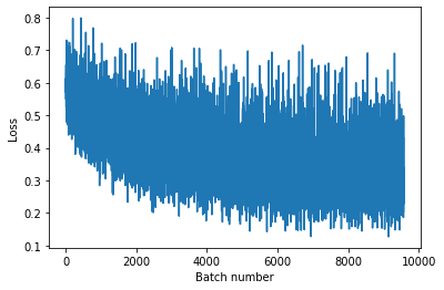
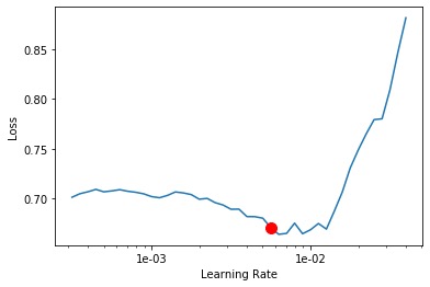
Submissions are evaluated on the log loss between the predicted values and the ground truth. By applying our FILM, we obtain a log loss score of 0.32141 from a single classifier (trained less than 20 minutes). The loss of the model decreased rapidly in the initial epochs but flattened out into a plateau as the number of training steps increased which is shown in Fig. 2.

Figure 1: Training loss is decreased when the numbers of training steps are increasing.

Figure 2: Find a best min numerical gradient of 5.62E-03.

Figure 3: Log loss of different sample in test dataset with hist() function.

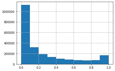
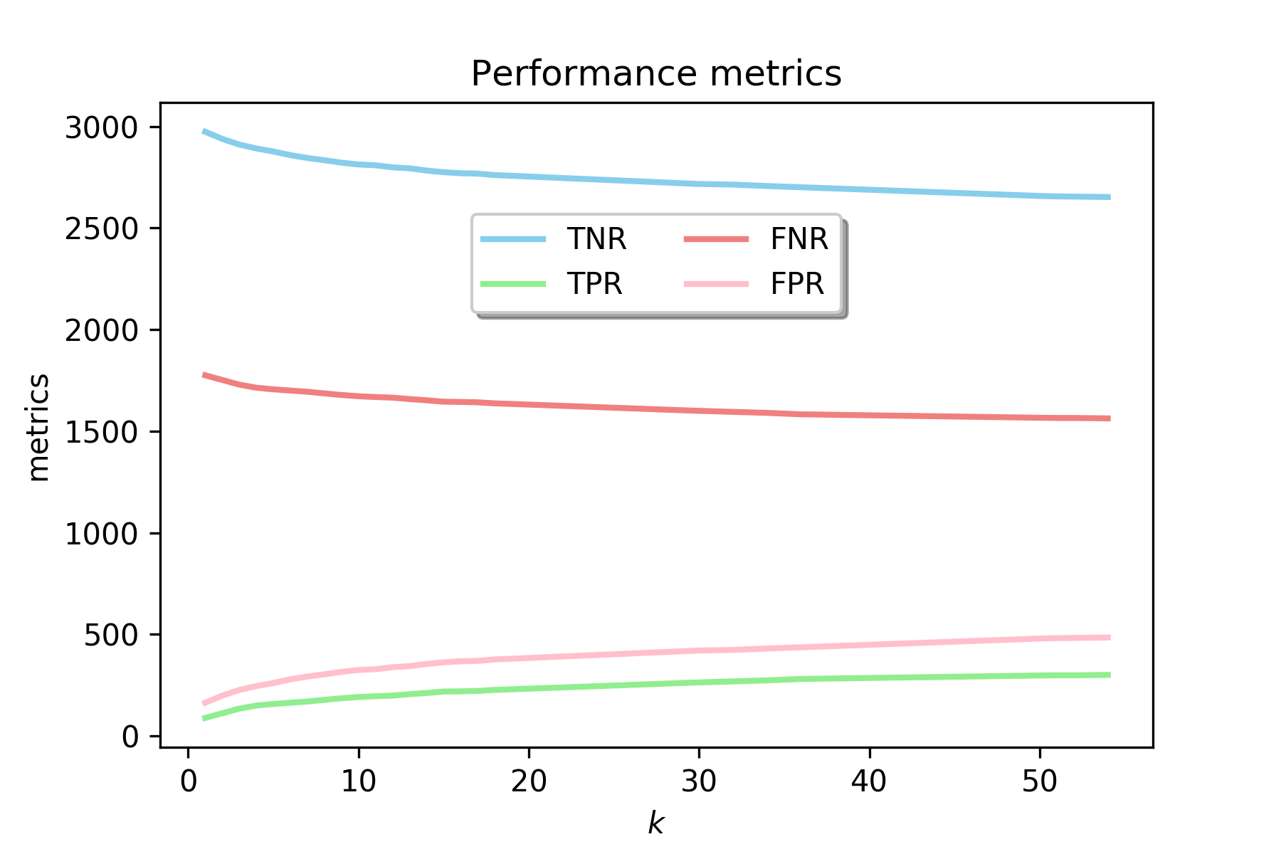
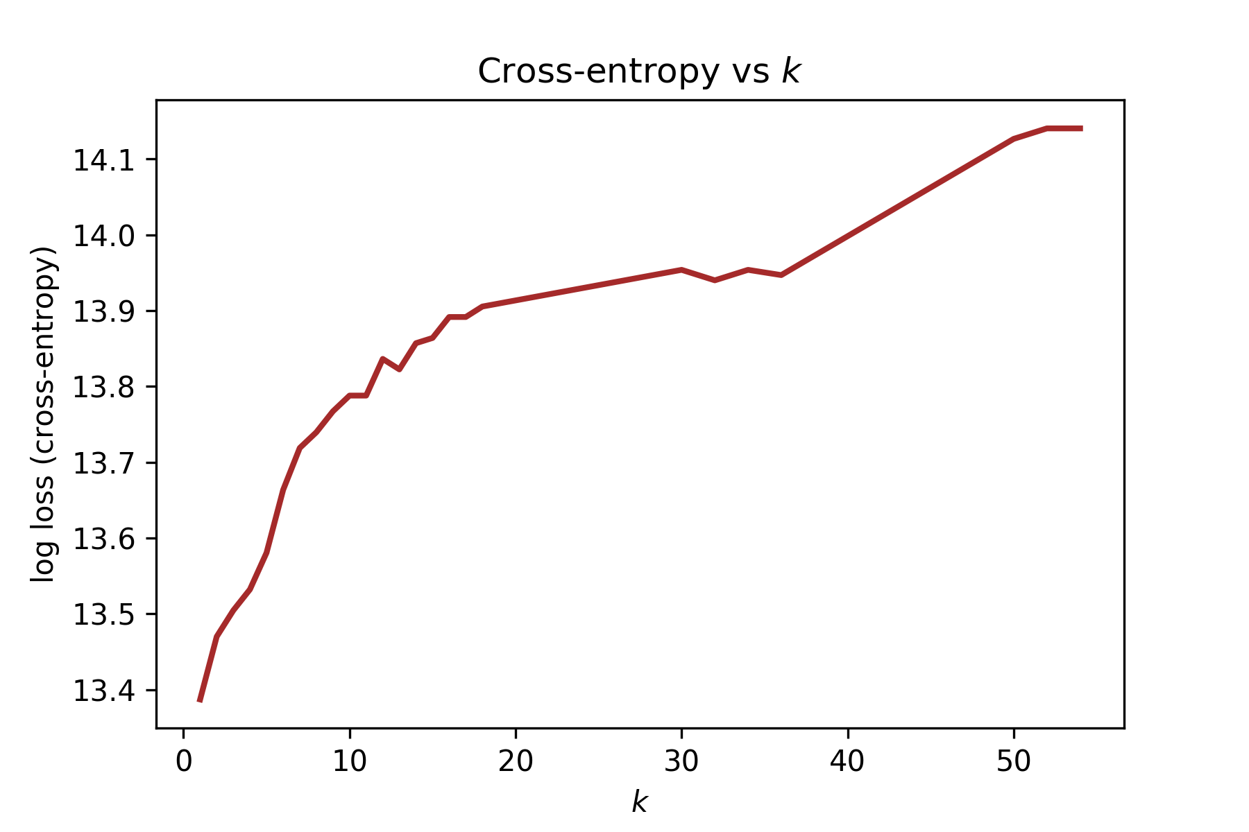
TF-IDF produced high-dimensional vectorizations $\mathbf{x}\in\mathbb{R}^{78113}$ of the training sentences. Setting $d=100$ and running FILM on the training set, we obtained a mapping $\mathbf{L}\in\mathbb{R}^{100\times 78113}$. We ran kNN for values of $k$ ranging from $1$ to $55$. For each value of $k$, we compute the cross-entropy loss (CE) and four other performance metrics: the True Positive Rate (TPR, defined as number of correctly classified similar pairs), True Negative Rate (TNR, defined as number of correctly classified dissimilar pairs), False Positive Rate (FPR) and False Negative Rate (FNR). We find that $k=1$ achieves the lowest CE, and the FNR does not decrease significantly as $k$ increases (see Figure2 below). Even though $k=1$ produces the lowest CE, we pick $k=36$ to run FILM on the test set, since there is an ‘‘elbow’’ in the CE for $k\geqslant 37$.

5 Analysis

After running the deep neural network, we find that our approaches have different strengths and weaknesses (Table 3). FILM is executable on a CPU, but we had to run the black box model on a GPU.

Figure 4: Metrics for performance of FILM on the validation set, $(\mathscr{S}_{\text{val}},\mathcal{P}_{\text{val}})$, as described in FILM Algorithm Step 6 of Section 3.2. (Top) TPR, TNR, FPR, FNR. (Bottom) Cross-entropy loss.

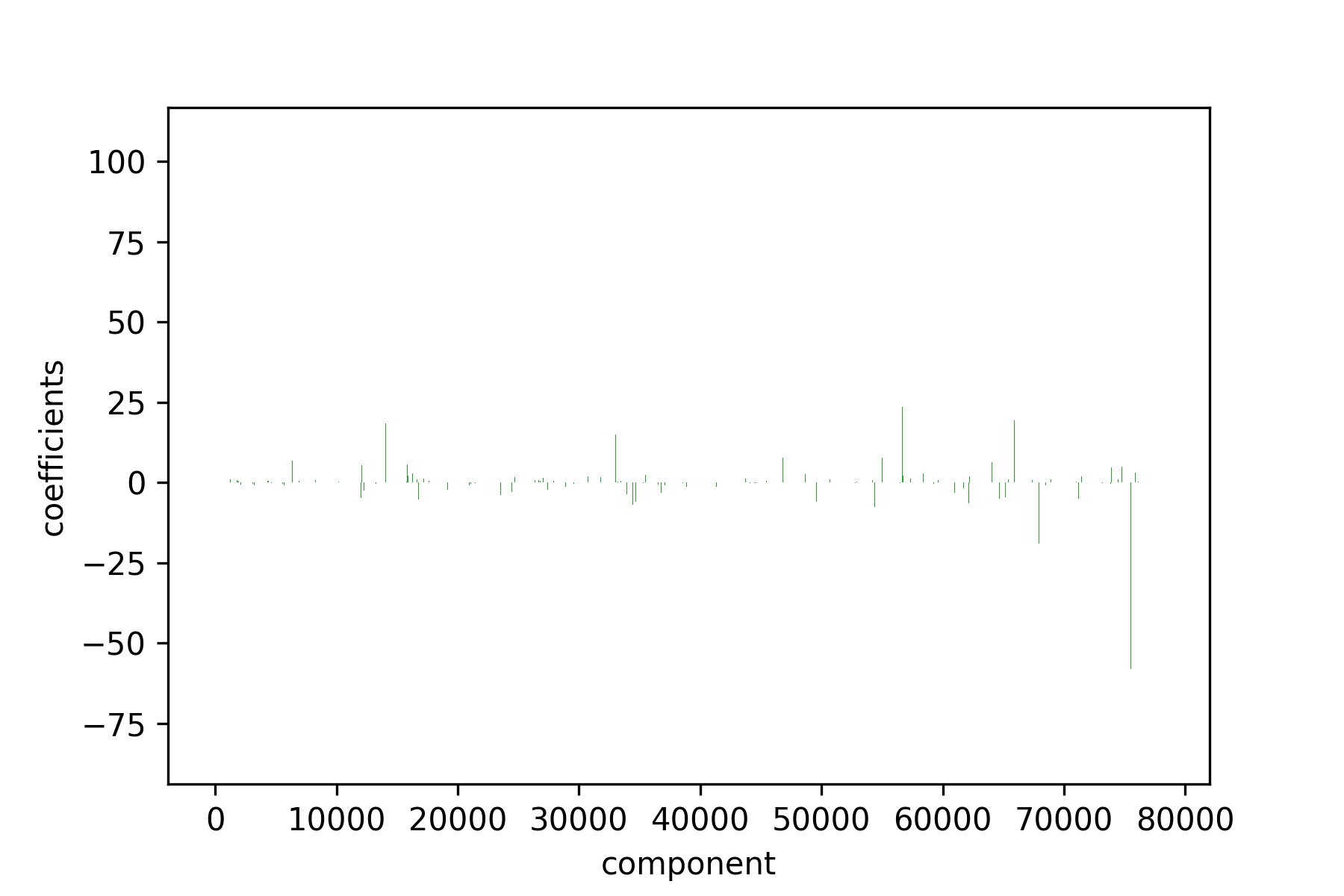
Finally, we find that the function learned on the black box model, $\phi$, lacks interpretability, whereas the mapping learned by FILM, $\mathbf{L}$, has a natural interpretation, as showed in Figure 5. Here, we observe that $\mathbf{l}_{1}$ has identified a small subset of features of $\mathbf{x}$. By comparing the nonzero indices of $\mathbf{l}_{1}$ with the corresponding word features in the TF-IDF embedding, we can identify if $\mathbf{l}_{1}$ has picked up any meaningful signal.

Figure 5: The $78113$ components of the first row of $\mathbf{L}$, which correspond to coefficients of the linear combination of $\mathbf{x}$ that determines the first component of the representation $\mathbf{y}$: $\mathbf{l}_{1}\mathbf{x}=y_{1}$.

The main unresolved problem of deep metric learning we found is overfitting. We can do detailed data analysis in the future to analyze the influence of selection bias and explore ways to select representative validation datasets. So the future work is to make metric learning more efficient to generalize model better. Also, it is hard to train, but we optimize it with N-Pair Loss. Moreover, the Quora dataset has a selection bias, which hurt the generalization performance of trained models and gives untrustworthy evaluation results. In other words, such train dataset leads to overfitting problem. In the future, we hope to propose frameworks that can improve the generalization ability of trained models, and give more trustworthy evaluation results for real-world adoptions.

Characteristic	Black Box Model	FILM
Memory Usage	Requires GPU	on CPU
Speed	$80$ minutes	$<30$ mins
Performance	SOTA	Strong
Interpretability	Weak	Strong

Table 3: Summary of strengths and weaknesses of the neural network model and FILM based on application to text matching data.

6 Conclusion

We investigated text matching, a core task in information retrieval and semantic analysis. We introduced the notation and definition of metric learning, and how it can be applied to text matching. Then, we explored FILM (Fast, Interpretable and Low-rank Metric learning), which aim to reduces the time cost and memory usage, also save energy consumption. In order to solve this task efficiently, FILM combined with a fast approximate k nearest neighbour search index. Compare to neural models, our method also has advantage in time and memory usage on large-scale and high-dimensional datasets.

References

- Absil and Malick (2012) Pierre-Antoine Absil and Jérôme Malick. 2012. Projection-like retractions on matrix manifolds. SIAM Journal on Optimization, 22(1):135--158.
- Barzilai and Borwein (1988) Jonathan Barzilai and Jonathan M Borwein. 1988. Two-point step size gradient methods. IMA Journal of Numerical Analysis, 8(1):141--148.
- Bogdanova et al. (2015) Dasha Bogdanova, Cicero dos Santos, Luciano Barbosa, and Bianca Zadrozny. 2015. Detecting semantically equivalent questions in online user forums. In Proceedings of the Nineteenth Conference on Computational Natural Language Learning, pages 123--131.
- Bonadiman et al. (2019) Daniele Bonadiman, Anjishnu Kumar, and Arpit Mittal. 2019. Large scale question paraphrase retrieval with smoothed deep metric learning. arXiv preprint arXiv:1905.12786.
- Bonadiman et al. (2017) Daniele Bonadiman, Antonio Uva, and Alessandro Moschitti. 2017. Multitask learning with deep neural networks for community question answering. arXiv preprint arXiv:1702.03706.
- Cheng (2013) Li Cheng. 2013. Riemannian similarity learning. In International Conference on Machine Learning, pages 540--548.
- Devlin et al. (2018) Jacob Devlin, Ming-Wei Chang, Kenton Lee, and Kristina Toutanova. 2018. Bert: Pre-training of deep bidirectional transformers for language understanding. arXiv preprint arXiv:1810.04805.
- Goldfarb et al. (2009) Donald Goldfarb, Zaiwen Wen, and Wotao Yin. 2009. A curvilinear search method for -harmonic flows on spheres. SIAM Journal on Imaging Sciences, 2(1):84--109.
- Harandi et al. (2017) Mehrtash Harandi, Mathieu Salzmann, and Richard Hartley. 2017. Joint dimensionality reduction and metric learning: A geometric take. In Proceedings of the 34th International Conference on Machine Learning-Volume 70, pages 1404--1413. JMLR. org.
- Hoffer and Ailon (2015) Elad Hoffer and Nir Ailon. 2015. Deep metric learning using triplet network. In International Workshop on Similarity-Based Pattern Recognition, pages 84--92. Springer.
- Huang et al. (2015) Zhiwu Huang, Ruiping Wang, Shiguang Shan, and Xilin Chen. 2015. Projection metric learning on grassmann manifold with application to video based face recognition. In Proceedings of the IEEE Conference on Computer Vision and Pattern Recognition, pages 140--149.
- Kim et al. (2019) Sungyeon Kim, Minkyo Seo, Ivan Laptev, Minsu Cho, and Suha Kwak. 2019. Deep metric learning beyond binary supervision. In Proceedings of the IEEE Conference on Computer Vision and Pattern Recognition, pages 2288--2297.
- Kwok and Tsang (2003) James T Kwok and Ivor W Tsang. 2003. Learning with idealized kernels. In Proceedings of the 20th International Conference on Machine Learning (ICML-03), pages 400--407.
- Liu et al. (2019) Han Liu, Zhizhong Han, Yu-Shen Liu, and Ming Gu. 2019. Fast low-rank metric learning for large-scale and high-dimensional data. In Advances in Neural Information Processing Systems, pages 817--827.
- Liu et al. (2015) Wei Liu, Cun Mu, Rongrong Ji, Shiqian Ma, John R Smith, and Shih-Fu Chang. 2015. Low-rank similarity metric learning in high dimensions. In Twenty-ninth AAAI conference on artificial intelligence.
- Mason et al. (2017) Blake Mason, Lalit Jain, and Robert Nowak. 2017. Learning low-dimensional metrics. In Advances in neural information processing systems, pages 4139--4147.
- Mikolov et al. (2013) Tomas Mikolov, Ilya Sutskever, Kai Chen, Greg S Corrado, and Jeff Dean. 2013. Distributed representations of words and phrases and their compositionality. In Advances in neural information processing systems, pages 3111--3119.
- Mu (2016) Yadong Mu. 2016. Fixed-rank supervised metric learning on riemannian manifold. In Thirtieth AAAI Conference on Artificial Intelligence.
- Nishimori and Akaho (2005) Yasunori Nishimori and Shotaro Akaho. 2005. Learning algorithms utilizing quasi-geodesic flows on the Stiefel manifold. Neurocomputing, 67:106--135.
- Pang et al. (2016) Liang Pang, Yanyan Lan, Jiafeng Guo, Jun Xu, Shengxian Wan, and Xueqi Cheng. 2016. Text matching as image recognition. In Thirtieth AAAI Conference on Artificial Intelligence.
- Salakhutdinov and Hinton (2009) Ruslan Salakhutdinov and Geoffrey Hinton. 2009. Semantic hashing. International Journal of Approximate Reasoning, 50(7):969--978.
- Schultz and Joachims (2004) Matthew Schultz and Thorsten Joachims. 2004. Learning a distance metric from relative comparisons. In Advances in neural information processing systems, pages 41--48.
- Wan et al. (2016) Shengxian Wan, Yanyan Lan, Jun Xu, Jiafeng Guo, Liang Pang, and Xueqi Cheng. 2016. Match-srnn: Modeling the recursive matching structure with spatial rnn. arXiv preprint arXiv:1604.04378.
- Wang et al. (2014) Jiang Wang, Yang Song, Thomas Leung, Chuck Rosenberg, Jingbin Wang, James Philbin, Bo Chen, and Ying Wu. 2014. Learning fine-grained image similarity with deep ranking. In Proceedings of the IEEE Conference on Computer Vision and Pattern Recognition, pages 1386--1393.
- Wang et al. (2017) Zhiguo Wang, Wael Hamza, and Radu Florian. 2017. Bilateral multi-perspective matching for natural language sentences. arXiv preprint arXiv:1702.03814.
- Zhang and Zhang (2017) Jie Zhang and Lijun Zhang. 2017. Efficient stochastic optimization for low-rank distance metric learning. In Thirty-First AAAI Conference on Artificial Intelligence.