State and parameter estimation from exact partial state observation in stochastic reaction networks

Muruhan Rathinam Department of Mathematics and Statistics, University of Maryland Baltimore County Mingkai Yu Department of Mathematics and Statistics, University of Maryland Baltimore County
Abstract

We consider chemical reaction networks modeled by a discrete state and continuous in time Markov process for the vector copy number of the species and provide a novel particle filter method for state and parameter estimation based on exact observation of some of the species in continuous time. The conditional probability distribution of the unobserved states is shown to satisfy a system of differential equations with jumps. We provide a method of simulating a process that is a proxy for the vector copy number of the unobserved species along with a weight. The resulting weighted Monte Carlo simulation is then used to compute the conditional probability distribution of the unobserved species. We also show how our algorithm can be adapted for a Bayesian estimation of parameters and for the estimation of a past state value based on observations up to a future time.

1 Introduction

Chemical reaction networks occurring at the intracellular level often have some or all molecular species present in low copy numbers. As such, these are best modeled by a discrete state Markov process in continuous time, where the state Z​(t)βˆˆβ„€+n𝑍𝑑superscriptsubscript℀𝑛Z(t)\in{\mathbb{Z}}_{+}^{n} of the process is the vector copy number of the molecular species at time t𝑑t. This model and the corresponding stochastic simulation algorithm introduced by Gillespie [18, 19] assumed a well-stirred system where spatial variations in molecular concentrations were considered negligible. Later on when the spatial variations were considered important, this model still proved useful in that its framework allowed for a spatial compartmental model where transport of molecules across compartments could be treated mathematically as reactions [6].

In this paper, we consider the problem of estimating the state Z​(t)𝑍𝑑Z(t) from exact and continuous observations of some of the states in time. In other words, suppose that the reaction network consists of n𝑛n molecular species where the vector copy number of n2subscript𝑛2n_{2} of the molecular species may be observed exactly as a function of time over the interval [0,t]0𝑑[0,t]. Based on this observation, we are interested in estimating the vector copy number of the remaining n1=nβˆ’n2subscript𝑛1𝑛subscript𝑛2n_{1}=n-n_{2} species at time t𝑑t. If we denote the vector copy number of the observable species by Y​(t)βˆˆβ„€+n2π‘Œπ‘‘superscriptsubscriptβ„€subscript𝑛2Y(t)\in{\mathbb{Z}}_{+}^{n_{2}} and that of the rest of the (unobservable) species by X​(t)βˆˆβ„€+n1𝑋𝑑superscriptsubscriptβ„€subscript𝑛1X(t)\in{\mathbb{Z}}_{+}^{n_{1}} (so that Z​(t)=(X​(t),Y​(t))π‘π‘‘π‘‹π‘‘π‘Œπ‘‘Z(t)=(X(t),Y(t))), then our goal is to compute the conditional probability distribution

π​(t,x)=P​{X​(t)=x|Y​(s)=y​(s), 0≀s≀t}πœ‹π‘‘π‘₯𝑃conditional-set𝑋𝑑π‘₯formulae-sequenceπ‘Œπ‘ π‘¦π‘ β€„0𝑠𝑑\pi(t,x)=P\{X(t)=x\,|\,Y(s)=y(s),\;0\leq s\leq t\}

for xβˆˆβ„€+n1π‘₯superscriptsubscriptβ„€subscript𝑛1x\in{\mathbb{Z}}_{+}^{n_{1}}.

Stochastic filtering methods provide a framework for addressing this type of problem, which is not restricted to reaction networks. The stochastic filtering methods usually involve generating recursive updates in time so that the additional computation required in going from the knowledge of conditional probability at a time instant t𝑑t to a future time instant t+hπ‘‘β„Žt+h only involves the observations made during (t,t+h]π‘‘π‘‘β„Ž(t,t+h] and the conditional probability computed by time t𝑑t. The widely known instance of stochastic filtering is the Kalman filter [27] which was concerned with a Gaussian process with a linear evolution in discrete time. Later on, the Kalman-Bucy filter [26] was introduced in the continuous time setting of linear stochastic differential equations (SDEs). In these linear and Gaussian settings the conditional probability distribution is also Gaussian, and hence its time evolution can be reduced to studying the time evolution of the mean and the covariance.

In general, one may not expect the conditional probability to be Gaussian and hence the methods are more complex. In the general nonlinear setting for SDEs there are several methods and one may find [4] as a general reference. In the setting of Markov processes in discrete time, one may find recursive filtering equations which describe the time evolution of the conditional probability distribution [14].

For discrete and finite state Markov processes in continuous time, a rigorous derivation of the evolution equation for the conditional probability distribution π​(t,x)πœ‹π‘‘π‘₯\pi(t,x) was provided in [10]. These evolution equations take the form of differential equations with jumps. These equations, known as the filtering equations, are analogous to Kolmogorov’s forward equations for the time evolution of the (unconditional) probability distribution P​{Z​(t)=z}𝑃𝑍𝑑𝑧P\{Z(t)=z\} of a continuous time and discrete state Markov process. In the case of reaction networks, Kolmogorov’s forward equations are known as the Chemical Master Equations (CME).

It is well known that when the number of states is infinite or very large, the solution of the CME is not practical and Monte Carlo simulation is the more efficient method of choice. The well known Gillespie algorithm [18, 21] and its variants[17, 1] are the methods of choice for exact realizations of sample paths. Likewise, when the state space for X​(t)𝑋𝑑X(t) is very large or infinite, direct numerical solution of the filtering equations is not practical.

As we shall describe in Section 2, the evolution equation for π​(t,x)πœ‹π‘‘π‘₯\pi(t,x) is nonlinear, and hence it is not possible to regard π​(t,x)πœ‹π‘‘π‘₯\pi(t,x) as the (unconditional) probability distribution of a Markov process. We shall define a nonnegative function ρ​(t,x)πœŒπ‘‘π‘₯\rho(t,x) which satisfies a linear evolution equation and when normalized yields π​(t,x)πœ‹π‘‘π‘₯\pi(t,x):

π​(t,x)=ρ​(t,x)βˆ‘x~ρ​(t,x~).πœ‹π‘‘π‘₯πœŒπ‘‘π‘₯subscript~π‘₯πœŒπ‘‘~π‘₯\pi(t,x)=\frac{\rho(t,x)}{\sum_{\tilde{x}}\rho(t,\tilde{x})}.

We refer to ρ​(t,x)πœŒπ‘‘π‘₯\rho(t,x) as the unnormalized conditional distribution and refer to the evolution equations (8) and (9) for ρ​(t,x)πœŒπ‘‘π‘₯\rho(t,x), that are defined in Section 2, as the unnormalized filtering equations. We shall show that ρ​(t,x)πœŒπ‘‘π‘₯\rho(t,x) equals the expected value of a function of a suitably defined Markov process (V​(t),w​(t))𝑉𝑑𝑀𝑑(V(t),w(t)):

ρ​(t,x)=𝔼​(1{x}​(V​(t))​w​(t)),πœŒπ‘‘π‘₯𝔼subscript1π‘₯𝑉𝑑𝑀𝑑\rho(t,x)={\mathbb{E}}\left(1_{\{x\}}(V(t))\,w(t)\right),

and thereby enabling an unbiased Monte Carlo estimate of ρ​(t,x)πœŒπ‘‘π‘₯\rho(t,x). Here, V𝑉V has β„€+n1superscriptsubscriptβ„€subscript𝑛1{\mathbb{Z}}_{+}^{n_{1}} as its state space (thus V𝑉V has the same state space as the unobserved species X𝑋X) and w𝑀w is a nonnegative weight.

To our best knowledge, in the context of discrete state and continuous time Markov chains, a Monte Carlo algorithm for the computation of π​(t,x)πœ‹π‘‘π‘₯\pi(t,x) based on an exact partial state trajectory y​(t)𝑦𝑑y(t) observed in continuous time, is not available in the literature. In this paper, we provide such a weighted Monte Carlo algorithm, also referred to as a particle filter, that is tailored to chemical reaction networks. Our algorithm provides an unbiased estimate of ρ​(t,x)πœŒπ‘‘π‘₯\rho(t,x), the unnormalized conditional distribution. The algorithm simulates Nssubscript𝑁𝑠N_{s} identically distributed copies of (V,w)𝑉𝑀(V,w) such that ρ​(t,x)πœŒπ‘‘π‘₯\rho(t,x) is estimated by

ρ^​(t,x)=1Nsβ€‹βˆ‘i=1Ns1{x}​(V(i)​(t))​w(i)​(t).^πœŒπ‘‘π‘₯1subscript𝑁𝑠superscriptsubscript𝑖1subscript𝑁𝑠subscript1π‘₯superscript𝑉𝑖𝑑superscript𝑀𝑖𝑑\hat{\rho}(t,x)=\frac{1}{N_{s}}\,\sum_{i=1}^{N_{s}}1_{\{x\}}(V^{(i)}(t))\,w^{(i)}(t).

Thus, π​(t,x)πœ‹π‘‘π‘₯\pi(t,x) is estimated by

Ο€^​(t,x)=βˆ‘i=1Ns1{x}​(V(i)​(t))​w(i)​(t)βˆ‘i=1Nsw(i)​(t).^πœ‹π‘‘π‘₯superscriptsubscript𝑖1subscript𝑁𝑠subscript1π‘₯superscript𝑉𝑖𝑑superscript𝑀𝑖𝑑superscriptsubscript𝑖1subscript𝑁𝑠superscript𝑀𝑖𝑑\hat{\pi}(t,x)=\frac{\sum_{i=1}^{N_{s}}1_{\{x\}}(V^{(i)}(t))\,w^{(i)}(t)}{\sum_{i=1}^{N_{s}}w^{(i)}(t)}.

Due to the division, Ο€^​(t,x)^πœ‹π‘‘π‘₯\hat{\pi}(t,x) is not an unbiased estimator of π​(t,x)πœ‹π‘‘π‘₯\pi(t,x). In fact, Monte Carlo methods of filtering in most other contexts (discrete time Markov chains, nonlinear SDEs etc.) also obtain the conditional probabilities by estimating an unnormalized version and then normalizing.

We describe some previous results for state and parameter estimation in the context of reaction networks. All these methods are for observations based on discrete time snapshots while our work addresses the case of continuous time observation. [7] considers Bayesian inference of parameters based on exact partial state observations in discrete time snapshots and proposes a Markov Chain Monte Carlo (MCMC) method. [22, 23] use the Chemical Langevin Equation (CLE) as the underlying model and propose MCMC methods for state and parameter estimation based on partial state observations corrupted by additive Gaussian noise in discrete time snapshots. [9] considers the case where the reaction network is approximated by the linear noise approximation. The observations are assumed to be linear combination of the states corrupted by an additive Gaussian noise with an unknown variance and they propose an extended Kalman-Bucy filter. They also consider pure delays in the system. The recent work in [13] considers the case where the reaction network may be approximated by an ODE model with jumps. A function of the state corrupted by an additive Gaussian noise is observed in discrete time snapshots. Rigorous results are derived to show that by solving the filtering problem for the reduced model based on observations of the original model, one can also obtain a good approximation of the estimation of the original model.

The weighted Monte Carlo method provided in this paper is concerned with the computation of the conditional distribution of the unobserved species based on exact observation of some species in continuous time. In reality, perfect observations are not possible. However, it is often reasonable to assume that the observation noise is discrete in nature and hence the noise could be incorporated into the model via the introduction of additional species and reactions. For instance, during fluorescence intensity observations, photons produced constitute a species and their production by a fluorescently tagged molecule constitutes a reaction channel. The assumption of continuous in time observation is less realistic. Nevertheless, if the sampling rate is high compared to reaction rates, then we expect this to provide a good approximation. Moreover, having an algorithm for the idealised baseline case of continuous in time observations is expected to provide valuable insights into how to analyse and develop techniques for the case of discrete time observations of a continuous time process.

The rest of the paper is organized as follows. In Section 2 we briefly review the basics of stochastic reaction networks and provide the filtering equations. We also introduce the useful unnormalized filtering equations. In Section 3 we provide a Monte Carlo filtering algorithm which generates a pair of processes (V,w)𝑉𝑀(V,w) where V𝑉V has the same state space as X𝑋X such that

π​(t,x)=𝔼​[1{x}​(V​(t))​w​(t)]𝔼​[w​(t)].πœ‹π‘‘π‘₯𝔼delimited-[]subscript1π‘₯𝑉𝑑𝑀𝑑𝔼delimited-[]𝑀𝑑\pi(t,x)=\frac{{\mathbb{E}}[1_{\{x\}}(V(t))\,w(t)]}{{\mathbb{E}}[w(t)]}.

We also show how our algorithm can be easily adapted to do parameter estimation based on exact partial state observation in a Bayesian framework and also how to estimate the conditional probability of a past event based on the observations made until a later time. That is, we show how to compute

P​{X​(t)=x|Y​(s)=y​(s), 0≀s≀T},𝑃conditional-set𝑋𝑑π‘₯formulae-sequenceπ‘Œπ‘ π‘¦π‘ β€‰0𝑠𝑇P\{X(t)=x\,|\,Y(s)=y(s),\,0\leq s\leq T\},

where xβˆˆβ„€+n1π‘₯superscriptsubscriptβ„€subscript𝑛1x\in{\mathbb{Z}}_{+}^{n_{1}} and 0<t<T0𝑑𝑇0<t<T, via an easy modification of our algorithm. In Section 5 we illustrate our algorithms via numerical examples and Section 6 makes some concluding remarks and discusses future work.

2 Stochastic reaction networks and filtering equations

We consider a stochastic reaction network with n𝑛n molecular species and mπ‘šm reaction channels. The process Z​(t)βˆˆβ„€+n𝑍𝑑superscriptsubscript℀𝑛Z(t)\in{\mathbb{Z}}_{+}^{n} stands for the copy number vector of the species at time t𝑑t. The dynamics of the reaction network are characterized by propensity functions aj​(z,c)subscriptπ‘Žπ‘—π‘§π‘a_{j}(z,c) where zβˆˆβ„€+n𝑧superscriptsubscript℀𝑛z\in{\mathbb{Z}}_{+}^{n} is the state and cβˆˆβ„p𝑐superscriptℝ𝑝c\in{\mathbb{R}}^{p} is a vector of parameters, and also by the stoichiometric vectors Ξ½jβˆˆβ„€nsubscriptπœˆπ‘—superscript℀𝑛\nu_{j}\in{\mathbb{Z}}^{n} for j=1,…,m𝑗1β€¦π‘šj=1,\dots,m. The occurrence of a reaction event j𝑗j at time t𝑑t leads to a state change Z​(t)=Z​(tβˆ’)+Ξ½j𝑍𝑑𝑍limit-from𝑑subscriptπœˆπ‘—Z(t)=Z(t-)+\nu_{j} and given Z​(t)=z𝑍𝑑𝑧Z(t)=z, the probability that a reaction event j𝑗j occurs during (t,t+h]π‘‘π‘‘β„Ž(t,t+h] is aj​(z,c)​h+o​(h)subscriptπ‘Žπ‘—π‘§π‘β„Žπ‘œβ„Ža_{j}(z,c)h+o(h) as hβ†’0+β†’β„Žlimit-from0h\to 0+. We shall adopt the convention that the process Z​(t)𝑍𝑑Z(t) is right continuous and assume Z​(t)𝑍𝑑Z(t) to be non-explosive, meaning that there are only finitely many reaction events during any finite time interval. For brevity, we suppress the dependence on parameters except when we are concerned with parameter estimation. It is well known[18, 21, 19, 21] that the time evolution of the (unconditional) probability mass function

p​(t,z)=P​{Z​(t)=z}𝑝𝑑𝑧𝑃𝑍𝑑𝑧p(t,z)=P\{Z(t)=z\}

is given by the Kolmogorov’s forward equations also known as the chemical master equations (CME):

p′​(t,z)=βˆ‘j=1maj​(zβˆ’Ξ½j)​p​(t,zβˆ’Ξ½j)βˆ’βˆ‘j=1maj​(z)​p​(t,z).superscript𝑝′𝑑𝑧superscriptsubscript𝑗1π‘šsubscriptπ‘Žπ‘—π‘§subscriptπœˆπ‘—π‘π‘‘π‘§subscriptπœˆπ‘—superscriptsubscript𝑗1π‘šsubscriptπ‘Žπ‘—π‘§π‘π‘‘π‘§p^{\prime}(t,z)=\sum_{j=1}^{m}a_{j}(z-\nu_{j})\,p(t,z-\nu_{j})-\sum_{j=1}^{m}a_{j}(z)\,p(t,z). (1)

We consider the situation where we make exact (noiseless) observations of the copy number of the last n2subscript𝑛2n_{2} species in continuous time. We write Z​(t)=(X​(t),Y​(t))π‘π‘‘π‘‹π‘‘π‘Œπ‘‘Z(t)=(X(t),Y(t)) where X​(t)βˆˆβ„€+n1𝑋𝑑superscriptsubscriptβ„€subscript𝑛1X(t)\in{\mathbb{Z}}_{+}^{n_{1}} is the unobserved component of the state and Y​(t)βˆˆβ„€+n2π‘Œπ‘‘superscriptsubscriptβ„€subscript𝑛2Y(t)\in{\mathbb{Z}}_{+}^{n_{2}} is the observed component of the state. Suppose we make a particular observation Y​(s)=y​(s)π‘Œπ‘ π‘¦π‘ Y(s)=y(s) for 0≀s≀t0𝑠𝑑0\leq s\leq t for tβ‰₯0𝑑0t\geq 0. We are interested in computing the conditional probability

π​(t,x)=P​{X​(t)=x|Y​(s)=y​(s), 0≀s≀t}βˆ€xβˆˆβ„€+n1.formulae-sequenceπœ‹π‘‘π‘₯𝑃conditional-set𝑋𝑑π‘₯formulae-sequenceπ‘Œπ‘ π‘¦π‘ β€‰0𝑠𝑑for-allπ‘₯superscriptsubscriptβ„€subscript𝑛1\pi(t,x)=P\{X(t)=x\,|\,Y(s)=y(s),\,0\leq s\leq t\}\quad\forall x\in{\mathbb{Z}}_{+}^{n_{1}}. (2)

Let us denote by Ξ½jβ€²subscriptsuperscriptπœˆβ€²π‘—\nu^{\prime}_{j} the first n1subscript𝑛1n_{1} components and by Ξ½jβ€²β€²subscriptsuperscriptπœˆβ€²β€²π‘—\nu^{\prime\prime}_{j} the last n2subscript𝑛2n_{2} components of Ξ½jsubscriptπœˆπ‘—\nu_{j} for j=1,…,m𝑗1β€¦π‘šj=1,\dots,m and define the subset π’ͺβŠ‚{1,…,m}π’ͺ1β€¦π‘š\mathcal{O}\subset\{1,\dots,m\} consisting of observable reaction channels, that is those that alter Y​(t)π‘Œπ‘‘Y(t). Thus j∈π’ͺ𝑗π’ͺj\in\mathcal{O} if and only if Ξ½jβ€²β€²β‰ 0subscriptsuperscriptπœˆβ€²β€²π‘—0\nu^{\prime\prime}_{j}\neq 0. We denote by 𝒰𝒰\mathcal{U}, the complement of π’ͺπ’ͺ\mathcal{O}. Thus 𝒰𝒰\mathcal{U} consists of the unobservable reaction channels.

We shall denote by tk,k=1,2,…formulae-sequencesubscriptπ‘‘π‘˜π‘˜12…t_{k},k=1,2,\dots the successive jump times of y​(t)𝑦𝑑y(t) and let t0=0subscript𝑑00t_{0}=0. Let’s define aπ’ͺ​(x,y)superscriptπ‘Žπ’ͺπ‘₯𝑦a^{\mathcal{O}}(x,y) and a𝒰​(x,y)superscriptπ‘Žπ’°π‘₯𝑦a^{\mathcal{U}}(x,y) by

aπ’ͺ​(x,y)=βˆ‘j∈π’ͺaj​(x,y),a𝒰​(x,y)=βˆ‘jβˆˆπ’°aj​(x,y),formulae-sequencesuperscriptπ‘Žπ’ͺπ‘₯𝑦subscript𝑗π’ͺsubscriptπ‘Žπ‘—π‘₯𝑦superscriptπ‘Žπ’°π‘₯𝑦subscript𝑗𝒰subscriptπ‘Žπ‘—π‘₯𝑦a^{\mathcal{O}}(x,y)=\sum_{j\in\mathcal{O}}a_{j}(x,y),\quad a^{\mathcal{U}}(x,y)=\sum_{j\in\mathcal{U}}a_{j}(x,y), (3)

which are respectively the total propensity of the observable and the unobservable reactions. For each kβˆˆβ„•π‘˜β„•k\in{\mathbb{N}} define π’ͺksubscriptπ’ͺπ‘˜\mathcal{O}_{k} by

π’ͺk={j∈π’ͺ|Ξ½jβ€²β€²=y​(tk)βˆ’y​(tkβˆ’)}.subscriptπ’ͺπ‘˜conditional-set𝑗π’ͺsubscriptsuperscriptπœˆβ€²β€²π‘—π‘¦subscriptπ‘‘π‘˜π‘¦limit-fromsubscriptπ‘‘π‘˜\mathcal{O}_{k}=\{j\in\mathcal{O}\,|\,\nu^{\prime\prime}_{j}=y(t_{k})-y(t_{k}-)\}.

Thus π’ͺksubscriptπ’ͺπ‘˜\mathcal{O}_{k} is the subset of observable reactions that are consistent with the observed jump y​(tk)βˆ’y​(tkβˆ’)=y​(tk)βˆ’y​(tkβˆ’1)𝑦subscriptπ‘‘π‘˜π‘¦limit-fromsubscriptπ‘‘π‘˜π‘¦subscriptπ‘‘π‘˜π‘¦subscriptπ‘‘π‘˜1y(t_{k})-y(t_{k}-)=y(t_{k})-y(t_{k-1}) at time tksubscriptπ‘‘π‘˜t_{k}.

The time evolution of π​(t,x)πœ‹π‘‘π‘₯\pi(t,x) follows a system of differential equations in between jump times tksubscriptπ‘‘π‘˜t_{k} and at the jump times π​(t,x)πœ‹π‘‘π‘₯\pi(t,x) undergoes jumps. A rigorous derivation of the evolution equations for π​(t,x)πœ‹π‘‘π‘₯\pi(t,x) (for finite state Markov processes) is given in [10] and we provide a more intuitive derivation in the Appendix. We summarize these equations which we call the filtering equations here.

For k=0,1,β€¦π‘˜01…k=0,1,\dots, and for tk≀t<tk+1subscriptπ‘‘π‘˜π‘‘subscriptπ‘‘π‘˜1t_{k}\leq t<t_{k+1}, Ο€πœ‹\pi satisfies the following system of differential equations:

π′​(t,x)superscriptπœ‹β€²π‘‘π‘₯\displaystyle\pi^{\prime}(t,x) =βˆ‘jβˆˆπ’°Ο€β€‹(t,xβˆ’Ξ½jβ€²)​aj​(xβˆ’Ξ½jβ€²,y​(tk))βˆ’βˆ‘jβˆˆπ’°Ο€β€‹(t,x)​aj​(x,y​(tk))absentsubscriptπ‘—π’°πœ‹π‘‘π‘₯superscriptsubscriptπœˆπ‘—β€²subscriptπ‘Žπ‘—π‘₯superscriptsubscriptπœˆπ‘—β€²π‘¦subscriptπ‘‘π‘˜subscriptπ‘—π’°πœ‹π‘‘π‘₯subscriptπ‘Žπ‘—π‘₯𝑦subscriptπ‘‘π‘˜\displaystyle=\sum_{j\in\mathcal{U}}\pi(t,x-\nu_{j}^{\prime})\,a_{j}(x-\nu_{j}^{\prime},y(t_{k}))-\sum_{j\in\mathcal{U}}\pi(t,x)\,a_{j}(x,y(t_{k})) (4)
βˆ’Ο€β€‹(t,x)​(aπ’ͺ​(x,y​(tk))βˆ’βˆ‘x~aπ’ͺ​(x~,y​(tk))​π​(t,x~))βˆ€xβˆˆβ„€+n1πœ‹π‘‘π‘₯superscriptπ‘Žπ’ͺπ‘₯𝑦subscriptπ‘‘π‘˜subscript~π‘₯superscriptπ‘Žπ’ͺ~π‘₯𝑦subscriptπ‘‘π‘˜πœ‹π‘‘~π‘₯for-allπ‘₯superscriptsubscriptβ„€subscript𝑛1\displaystyle-\pi(t,x)\left(a^{\mathcal{O}}(x,y(t_{k}))-\sum_{\tilde{x}}a^{\mathcal{O}}(\tilde{x},y(t_{k}))\pi(t,\tilde{x})\right)\quad\forall x\in{\mathbb{Z}}_{+}^{n_{1}}

and for k=1,2,β€¦π‘˜12…k=1,2,\dots, and at times tksubscriptπ‘‘π‘˜t_{k}, π​(t,x)πœ‹π‘‘π‘₯\pi(t,x) jumps according to:

π​(tk,x)=βˆ‘l∈π’ͺkal​(xβˆ’Ξ½lβ€²,y​(tkβˆ’1))​π​(tkβˆ’,xβˆ’Ξ½lβ€²)βˆ‘x~βˆ‘l∈π’ͺkal​(x~,y​(tkβˆ’1))​π​(tkβˆ’,x~)βˆ€xβˆˆβ„€+n1.formulae-sequenceπœ‹subscriptπ‘‘π‘˜π‘₯subscript𝑙subscriptπ’ͺπ‘˜subscriptπ‘Žπ‘™π‘₯superscriptsubscriptπœˆπ‘™β€²π‘¦subscriptπ‘‘π‘˜1πœ‹limit-fromsubscriptπ‘‘π‘˜π‘₯superscriptsubscriptπœˆπ‘™β€²subscript~π‘₯subscript𝑙subscriptπ’ͺπ‘˜subscriptπ‘Žπ‘™~π‘₯𝑦subscriptπ‘‘π‘˜1πœ‹limit-fromsubscriptπ‘‘π‘˜~π‘₯for-allπ‘₯superscriptsubscriptβ„€subscript𝑛1\pi(t_{k},x)=\frac{\sum_{l\in\mathcal{O}_{k}}a_{l}(x-\nu_{l}^{\prime},y(t_{k-1}))\,\pi(t_{k}-,x-\nu_{l}^{\prime})}{\sum_{\tilde{x}}\sum_{l\in\mathcal{O}_{k}}a_{l}(\tilde{x},y(t_{k-1}))\,\pi(t_{k}-,\tilde{x})}\quad\forall x\in{\mathbb{Z}}_{+}^{n_{1}}. (5)

We note that π​(t,x)πœ‹π‘‘π‘₯\pi(t,x) is right continuous since by our convention the process Z​(t)𝑍𝑑Z(t) is right continuous and as a consequence the observed trajectory y​(t)𝑦𝑑y(t) is right continuous as well.

Since we are interested in the case where the state space of the system of ODEs (4) is either an infinite or a very large finite subset of β„€+n1superscriptsubscriptβ„€subscript𝑛1{\mathbb{Z}}_{+}^{n_{1}}, a direct solution of this equation is not practical. Instead our goal is a Monte Carlo simulation. Our Monte Carlo algorithm involves generating a trajectory V​(t)𝑉𝑑V(t) with same state space β„€+n1superscriptsubscriptβ„€subscript𝑛1{\mathbb{Z}}_{+}^{n_{1}} as X​(t)𝑋𝑑X(t), along with a weight trajectory w​(t)𝑀𝑑w(t), such that at any time tβ‰₯0𝑑0t\geq 0 and for xβˆˆβ„€+n1π‘₯superscriptsubscriptβ„€subscript𝑛1x\in{\mathbb{Z}}_{+}^{n_{1}}

π​(t,x)=𝔼​[w​(t)​1{x}​(V​(t))]𝔼​[w​(t)].πœ‹π‘‘π‘₯𝔼delimited-[]𝑀𝑑subscript1π‘₯𝑉𝑑𝔼delimited-[]𝑀𝑑\pi(t,x)=\frac{{\mathbb{E}}[w(t)1_{\{x\}}(V(t))]}{{\mathbb{E}}[w(t)]}. (6)

We note that, given a set A𝐴A, 1Asubscript1𝐴1_{A} is the indicator function of the set. In practice, from a sample of Nssubscript𝑁𝑠N_{s} identically distributed trajectories V(i)superscript𝑉𝑖V^{(i)} along with weights w(i)superscript𝑀𝑖w^{(i)} for i=1,…,Ns𝑖1…subscript𝑁𝑠i=1,\dots,N_{s}, π​(t,x)πœ‹π‘‘π‘₯\pi(t,x) is estimated by

Ο€^​(t,x)=βˆ‘i=1Ns1{x}​(V(i)​(t))​w(i)​(t)βˆ‘i=1Nsw(i)​(t)^πœ‹π‘‘π‘₯superscriptsubscript𝑖1subscript𝑁𝑠subscript1π‘₯superscript𝑉𝑖𝑑superscript𝑀𝑖𝑑superscriptsubscript𝑖1subscript𝑁𝑠superscript𝑀𝑖𝑑\hat{\pi}(t,x)=\frac{\sum_{i=1}^{N_{s}}1_{\{x\}}(V^{(i)}(t))\,w^{(i)}(t)}{\sum_{i=1}^{N_{s}}w^{(i)}(t)} (7)

Since (4) is not linear, Ο€πœ‹\pi cannot be interpreted as the probability mass function of some Markov process. However, we can define a related quantity ρ​(t,x)πœŒπ‘‘π‘₯\rho(t,x) which evolves according to a linear equation and can be related to a Markov process. We define ρ​(t,x)πœŒπ‘‘π‘₯\rho(t,x) to be a nonnegative function that satisfies the unnormalized filtering equations defined as below.

For k=0,1,β€¦π‘˜01…k=0,1,\dots on the interval tk≀t<tk+1subscriptπ‘‘π‘˜π‘‘subscriptπ‘‘π‘˜1t_{k}\leq t<t_{k+1}, ρ​(x,t)𝜌π‘₯𝑑\rho(x,t) satisfies

ρ′​(t,x)superscriptπœŒβ€²π‘‘π‘₯\displaystyle\rho^{\prime}(t,x) =βˆ‘jβˆˆπ’°Οβ€‹(t,xβˆ’Ξ½jβ€²)​aj​(xβˆ’Ξ½jβ€²,y​(tk))βˆ’βˆ‘jβˆˆπ’°Οβ€‹(t,x)​aj​(x,y​(tk))absentsubscriptπ‘—π’°πœŒπ‘‘π‘₯superscriptsubscriptπœˆπ‘—β€²subscriptπ‘Žπ‘—π‘₯superscriptsubscriptπœˆπ‘—β€²π‘¦subscriptπ‘‘π‘˜subscriptπ‘—π’°πœŒπ‘‘π‘₯subscriptπ‘Žπ‘—π‘₯𝑦subscriptπ‘‘π‘˜\displaystyle=\sum_{j\in\mathcal{U}}\rho(t,x-\nu_{j}^{\prime})\,a_{j}(x-\nu_{j}^{\prime},y(t_{k}))-\sum_{j\in\mathcal{U}}\rho(t,x)\,a_{j}(x,y(t_{k})) (8)
βˆ’Οβ€‹(t,x)​aπ’ͺ​(x,y​(tk))βˆ€xβˆˆβ„€+n1.πœŒπ‘‘π‘₯superscriptπ‘Žπ’ͺπ‘₯𝑦subscriptπ‘‘π‘˜for-allπ‘₯superscriptsubscriptβ„€subscript𝑛1\displaystyle-\rho(t,x)\,a^{\mathcal{O}}(x,y(t_{k}))\quad\forall x\in{\mathbb{Z}}_{+}^{n_{1}}.

For k=1,2,β€¦π‘˜12…k=1,2,\dots at jump times tksubscriptπ‘‘π‘˜t_{k}, ρ​(t,x)πœŒπ‘‘π‘₯\rho(t,x) jumps according to

ρ​(tk,x)=1|π’ͺk|β€‹βˆ‘j∈π’ͺkaj​(xβˆ’Ξ½jβ€²,y​(tkβˆ’1))​ρ​(tkβˆ’,xβˆ’Ξ½jβ€²)xβˆˆβ„€+n1.formulae-sequence𝜌subscriptπ‘‘π‘˜π‘₯1subscriptπ’ͺπ‘˜subscript𝑗subscriptπ’ͺπ‘˜subscriptπ‘Žπ‘—π‘₯superscriptsubscriptπœˆπ‘—β€²π‘¦subscriptπ‘‘π‘˜1𝜌limit-fromsubscriptπ‘‘π‘˜π‘₯superscriptsubscriptπœˆπ‘—β€²π‘₯superscriptsubscriptβ„€subscript𝑛1\rho(t_{k},x)=\frac{1}{|\mathcal{O}_{k}|}\sum_{j\in\mathcal{O}_{k}}a_{j}(x-\nu_{j}^{\prime},y(t_{k-1}))\,\rho(t_{k}-,x-\nu_{j}^{\prime})\quad x\in{\mathbb{Z}}_{+}^{n_{1}}. (9)

We note that |π’ͺk|subscriptπ’ͺπ‘˜|\mathcal{O}_{k}| is the number of reaction channels in the set π’ͺksubscriptπ’ͺπ‘˜\mathcal{O}_{k} and this is non-zero. Let ρ¯​(t)=βˆ‘x~ρ​(t,x~)Β―πœŒπ‘‘subscript~π‘₯πœŒπ‘‘~π‘₯\bar{\rho}(t)=\sum_{\tilde{x}}\rho(t,\tilde{x}). It is shown in Appendix B that Ο€πœ‹\pi is given by π​(t,x)=ρ​(t,x)/ρ¯​(t)πœ‹π‘‘π‘₯πœŒπ‘‘π‘₯Β―πœŒπ‘‘\pi(t,x)=\rho(t,x)/\bar{\rho}(t). In the next section we shall see that an appropriate stochastic interpretation of ρ​(t,x)πœŒπ‘‘π‘₯\rho(t,x) leads to the stochastic simulation algorithm to generate V𝑉V and w𝑀w such that

𝔼​[1{x}​(V​(t))​w​(t)]=ρ​(t,x).𝔼delimited-[]subscript1π‘₯π‘‰π‘‘π‘€π‘‘πœŒπ‘‘π‘₯{\mathbb{E}}\left[1_{\{x\}}(V(t))\,w(t)\right]=\rho(t,x). (10)

3 Monte Carlo Algorithms

3.1 Weighted Monte Carlo and Resampling

In Section 3.2 we shall define a pair of processes (V,w)𝑉𝑀(V,w) with state space β„€+n1Γ—[0,∞)superscriptsubscriptβ„€subscript𝑛10{\mathbb{Z}}_{+}^{n_{1}}\times[0,\infty) such that (10) holds where ρ𝜌\rho satisfies the unnormalized filtering equations (8) and (9). The estimation of π​(t,x)πœ‹π‘‘π‘₯\pi(t,x) is accomplished by simulating Nssubscript𝑁𝑠N_{s} identically distributed copies of the pair of processes (V,w)𝑉𝑀(V,w) and estimating π​(t,x)πœ‹π‘‘π‘₯\pi(t,x) via (7).

We note that this type of procedure differs from the most common form of simulating a reaction network via Nssubscript𝑁𝑠N_{s} i.i.d.Β trajectories, say Z(i)superscript𝑍𝑖Z^{(i)} and then estimating 𝔼​[φ​(Z​(t))]𝔼delimited-[]πœ‘π‘π‘‘{\mathbb{E}}[\varphi(Z(t))], the expectation of a function Ο†πœ‘\varphi of the state via the sample average

1Nsβ€‹βˆ‘i=1Nsφ​(Z(i)​(t)).1subscript𝑁𝑠superscriptsubscript𝑖1subscriptπ‘π‘ πœ‘superscript𝑍𝑖𝑑\frac{1}{N_{s}}\sum_{i=1}^{N_{s}}\varphi(Z^{(i)}(t)).

In this most familiar form of Monte Carlo simulation, all trajectories are weighted equally. In our situation, the Monte Carlo algorithm involves a weighted average. The weights carry information about the relative importance of trajectories of V𝑉V.

Corresponding to the sample (V(i),w(i))superscript𝑉𝑖superscript𝑀𝑖(V^{(i)},w^{(i)}) where i=1,…,Ns𝑖1…subscript𝑁𝑠i=1,\dots,N_{s}, we may associate the (random) empirical measure (mass) M​(t)𝑀𝑑M(t) at time t𝑑t given by

M​(t)=1Nsβ€‹βˆ‘i=1Nsw(i)​(t)​δV(i)​(t),𝑀𝑑1subscript𝑁𝑠superscriptsubscript𝑖1subscript𝑁𝑠superscript𝑀𝑖𝑑subscript𝛿superscript𝑉𝑖𝑑M(t)=\frac{1}{N_{s}}\sum_{i=1}^{N_{s}}w^{(i)}(t)\,\delta_{V^{(i)}(t)}, (11)

where Ξ΄xsubscript𝛿π‘₯\delta_{x} stands for the Dirac mass or unit point mass concentrated at xβˆˆβ„€+n1π‘₯superscriptsubscriptβ„€subscript𝑛1x\in{\mathbb{Z}}_{+}^{n_{1}}. If we choose (V,w)𝑉𝑀(V,w) to satisfy (10), then for each xβˆˆβ„€+n1π‘₯superscriptsubscriptβ„€subscript𝑛1x\in{\mathbb{Z}}_{+}^{n_{1}} the expected value of the empirical measure of the singleton {x}π‘₯\{x\} is ρ​(t,x)πœŒπ‘‘π‘₯\rho(t,x):

𝔼​[M​(t)​({x})]=ρ​(t,x).𝔼delimited-[]𝑀𝑑π‘₯πœŒπ‘‘π‘₯{\mathbb{E}}[M(t)(\{x\})]=\rho(t,x). (12)

The fact that the weights may grow (or decay) unevenly as time progresses leads to two different issues. The first issue is that the simulation may run into numerical problems where some weights become very large while others become very small, exceeding the finite precision of the computer. Especially, very large weights will become Inf in the finite precision representation of the computer, rendering computations impractical. The second issue is more fundamental and is unrelated to the finite precision nature of computations. The accuracy of the Monte Carlo estimate of π​(t,x)πœ‹π‘‘π‘₯\pi(t,x) depends on the variance of w​(t)𝑀𝑑w(t) as well as the variance of 1{x}​(V​(t))​w​(t)subscript1π‘₯𝑉𝑑𝑀𝑑1_{\{x\}}(V(t))\,w(t) and also the covariance between these two terms. If the algorithm allows for a large variance in w​(t)𝑀𝑑w(t), naturally this would have negative implications for the accuracy of the estimate.

In order to avoid these issues, one may resample the empirical measure at certain time points to produce a new empirical measure that is still the sum of Nssubscript𝑁𝑠N_{s} Dirac masses but with equal weights. By resampling, we mean the creation a new weighted sample of size Nssubscript𝑁𝑠N_{s} from an existing weighted sample of size Nssubscript𝑁𝑠N_{s} that captures the information in the original sample. In particular, if an empirical measure M​(t)𝑀𝑑M(t) at time t𝑑t is resampled to produce another empirical measure M~​(t)~𝑀𝑑\tilde{M}(t), then we want the resampling procedure to satisfy the basic condition that

𝔼​[M~​(t)​({x})]=𝔼​[M​(t)​({x})]βˆ€xβˆˆβ„€+n1.formulae-sequence𝔼delimited-[]~𝑀𝑑π‘₯𝔼delimited-[]𝑀𝑑π‘₯for-allπ‘₯superscriptsubscriptβ„€subscript𝑛1{\mathbb{E}}[\tilde{M}(t)(\{x\})]={\mathbb{E}}[M(t)(\{x\})]\quad\forall x\in{\mathbb{Z}}_{+}^{n_{1}}. (13)

In order to maintain above requirement, the resampling procedure itself introduces extra randomness which in turn can result in loss of accuracy. Thus the frequency with which resampling is performed will be an important topic of investigation. We also note that the resampling procedure introduces dependence among the sample trajectories. Thus, while (V(i),w(i))superscript𝑉𝑖superscript𝑀𝑖(V^{(i)},w^{(i)}) for i=1,…,Ns𝑖1…subscript𝑁𝑠i=1,\dots,N_{s} are identically distributed, the collection is not necessarily independent.

Suppose that at time t0>0subscript𝑑00t_{0}>0, we have simulated pairs (V(i)​(t0),w(i)​(t0))superscript𝑉𝑖subscript𝑑0superscript𝑀𝑖subscript𝑑0(V^{(i)}(t_{0}),w^{(i)}(t_{0})) for i=1,…,Ns𝑖1…subscript𝑁𝑠i=1,\dots,N_{s}, and we resample to produce a new set of pairs (V~(i)​(t0),w~(i)​(t0))superscript~𝑉𝑖subscript𝑑0superscript~𝑀𝑖subscript𝑑0(\tilde{V}^{(i)}(t_{0}),\tilde{w}^{(i)}(t_{0})) for i=1,…,Ns𝑖1…subscript𝑁𝑠i=1,\dots,N_{s}. Then we shall have that for all i𝑖i and j𝑗j,

𝔼​[1{x}​(V~(j)​(t0))​w~(j)​(t0)]=𝔼​[1{x}​(V(i)​(t0))​w(i)​(t0)],𝔼delimited-[]subscript1π‘₯superscript~𝑉𝑗subscript𝑑0superscript~𝑀𝑗subscript𝑑0𝔼delimited-[]subscript1π‘₯superscript𝑉𝑖subscript𝑑0superscript𝑀𝑖subscript𝑑0{\mathbb{E}}[1_{\{x\}}(\tilde{V}^{(j)}(t_{0}))\,\tilde{w}^{(j)}(t_{0})]={\mathbb{E}}[1_{\{x\}}(V^{(i)}(t_{0}))\,w^{(i)}(t_{0})],

and w~(j)​(t0)=1superscript~𝑀𝑗subscript𝑑01\tilde{w}^{(j)}(t_{0})=1 for j=1,…,Ns𝑗1…subscript𝑁𝑠j=1,\dots,N_{s}. The consequent evolution of (V~(j)​(t),w~(j)​(t))superscript~𝑉𝑗𝑑superscript~𝑀𝑗𝑑(\tilde{V}^{(j)}(t),\tilde{w}^{(j)}(t)) for j=1,…,Ns𝑗1…subscript𝑁𝑠j=1,\dots,N_{s} (which we shall rename (V(j),w(j))superscript𝑉𝑗superscript𝑀𝑗(V^{(j)},w^{(j)})), will proceed in a conditionally independent fashion until the next resampling.

We shall employ a particular resampling algorithm described in [4] and Β [11]. This is given in Algorithm 4 and involves regarding each sample point/particle as giving birth to a number (possibly zero) of offsprings. It is most convenient to think of this algorithm as propagating Nssubscript𝑁𝑠N_{s} particles so that at time t𝑑t, the i𝑖ith particle is situated at location V(i)​(t)βˆˆβ„€+n1superscript𝑉𝑖𝑑superscriptsubscriptβ„€subscript𝑛1V^{(i)}(t)\in{\mathbb{Z}}_{+}^{n_{1}} and has weight w(i)​(t)β‰₯0superscript𝑀𝑖𝑑0w^{(i)}(t)\geq 0. When resampling occurs at say, time t0subscript𝑑0t_{0}, Algorithm 4 considers the weight of each particle i𝑖i and assigns a random number o(i)βˆˆβ„€+superscriptπ‘œπ‘–subscriptβ„€o^{(i)}\in{\mathbb{Z}}_{+} of offsprings to the particle. The number o(i)superscriptπ‘œπ‘–o^{(i)} is chosen such that 𝔼​[o(i)|w(i)​(t0)]=w(i)​(t0)𝔼delimited-[]conditionalsuperscriptπ‘œπ‘–superscript𝑀𝑖subscript𝑑0superscript𝑀𝑖subscript𝑑0{\mathbb{E}}[o^{(i)}\,|\,w^{(i)}(t_{0})]=w^{(i)}(t_{0}) and subject to the condition that the total number of offsprings of all particles is Nssubscript𝑁𝑠N_{s}. Each particle i𝑖i is considered β€œdead” after it gives β€œbirth” to o(i)superscriptπ‘œπ‘–o^{(i)} offsprings each of which start at the same location V(i)​(t0)superscript𝑉𝑖subscript𝑑0V^{(i)}(t_{0}) as its parent and with weight w(i)​(t0)=1superscript𝑀𝑖subscript𝑑01w^{(i)}(t_{0})=1. Subsequently all the offsprings evolve independently. We refer the reader to [4] (Section 9.2) and [11] regarding further details of a specific version of this algorithm that is also used by us and described in Algorithm 4.

3.2 Processes V𝑉V and w𝑀w

In this section we define a pair of processes (V,w)𝑉𝑀(V,w) where V​(t)βˆˆβ„€+n1𝑉𝑑superscriptsubscriptβ„€subscript𝑛1V(t)\in{\mathbb{Z}}_{+}^{n_{1}} and w​(t)β‰₯0𝑀𝑑0w(t)\geq 0 as follows. We initialize V​(0)𝑉0V(0) with the same distribution as that of the initial state X​(0)=x0𝑋0subscriptπ‘₯0X(0)=x_{0} and set w​(0)=1𝑀01w(0)=1. In between jump times, that is, for tk≀t<tk+1subscriptπ‘‘π‘˜π‘‘subscriptπ‘‘π‘˜1t_{k}\leq t<t_{k+1} where k=0,1,β€¦π‘˜01…k=0,1,\dots, the process V𝑉V is evolved according to the underlying reaction network with all observable reactions removed. Thus only the copy number of the first n1subscript𝑛1n_{1} species can change during (tk,tk+1)subscriptπ‘‘π‘˜subscriptπ‘‘π‘˜1(t_{k},t_{k+1}). Moreover, for tk≀t<tk+1subscriptπ‘‘π‘˜π‘‘subscriptπ‘‘π‘˜1t_{k}\leq t<t_{k+1} where k=0,1,β€¦π‘˜01…k=0,1,\dots, the weight process w​(t)𝑀𝑑w(t) is evolved according to

w​(t)=w​(tk)​exp⁑{βˆ’βˆ«tktaπ’ͺ​(V​(s),y​(tk))​𝑑s}.𝑀𝑑𝑀subscriptπ‘‘π‘˜superscriptsubscriptsubscriptπ‘‘π‘˜π‘‘superscriptπ‘Žπ’ͺ𝑉𝑠𝑦subscriptπ‘‘π‘˜differential-d𝑠w(t)=w(t_{k})\,\exp\left\{-\int_{t_{k}}^{t}a^{\mathcal{O}}(V(s),y(t_{k}))\,ds\right\}. (14)

Equivalently, we note that w​(t)𝑀𝑑w(t) satisfies the ODE

w′​(t)=w​(t)​aπ’ͺ​(V​(t),y​(tk))superscript𝑀′𝑑𝑀𝑑superscriptπ‘Žπ’ͺ𝑉𝑑𝑦subscriptπ‘‘π‘˜w^{\prime}(t)=w(t)\,a^{\mathcal{O}}(V(t),y(t_{k}))

for tk≀t<tk+1subscriptπ‘‘π‘˜π‘‘subscriptπ‘‘π‘˜1t_{k}\leq t<t_{k+1} (at t=tk𝑑subscriptπ‘‘π‘˜t=t_{k} the right-hand side derivative is considered). At jump times t=tk𝑑subscriptπ‘‘π‘˜t=t_{k} for k=1,2,β€¦π‘˜12…k=1,2,\dots the process w​(t)𝑀𝑑w(t) jumps as follows. For j∈π’ͺk𝑗subscriptπ’ͺπ‘˜j\in\mathcal{O}_{k}, set

w​(tk)=w​(tkβˆ’)​aj​(V​(tkβˆ’),y​(tkβˆ’1))​ with probability ​1|π’ͺk|.𝑀subscriptπ‘‘π‘˜π‘€limit-fromsubscriptπ‘‘π‘˜subscriptπ‘Žπ‘—π‘‰limit-fromsubscriptπ‘‘π‘˜π‘¦subscriptπ‘‘π‘˜1Β with probabilityΒ 1subscriptπ’ͺπ‘˜w(t_{k})=w(t_{k}-)\,a_{j}(V(t_{k}-),y(t_{k-1}))\;\;\text{ with probability }\frac{1}{|\mathcal{O}_{k}|}. (15)

Moreover, at jump times t=tk𝑑subscriptπ‘‘π‘˜t=t_{k} for k=1,2,β€¦π‘˜12…k=1,2,\dots the process V​(t)𝑉𝑑V(t) jumps as follows. For j∈π’ͺk𝑗subscriptπ’ͺπ‘˜j\in\mathcal{O}_{k}, set

V​(tk)=V​(tkβˆ’)+Ξ½j′​ with probability ​1|π’ͺk|.𝑉subscriptπ‘‘π‘˜π‘‰limit-fromsubscriptπ‘‘π‘˜superscriptsubscriptπœˆπ‘—β€²Β with probabilityΒ 1subscriptπ’ͺπ‘˜V(t_{k})=V(t_{k}-)+\nu_{j}^{\prime}\;\;\text{ with probability }\frac{1}{|\mathcal{O}_{k}|}. (16)

We note that if aj​(V​(tkβˆ’),y​(tkβˆ’1))=0subscriptπ‘Žπ‘—π‘‰limit-fromsubscriptπ‘‘π‘˜π‘¦subscriptπ‘‘π‘˜10a_{j}(V(t_{k}-),y(t_{k-1}))=0 for the chosen j∈π’ͺk𝑗subscriptπ’ͺπ‘˜j\in\mathcal{O}_{k}, it may be possible that V​(tk)𝑉subscriptπ‘‘π‘˜V(t_{k}) is assigned an infeasible state, that is a state that has negative components. However, at the same time w​(tk)𝑀subscriptπ‘‘π‘˜w(t_{k}) would be zero and hence the value of V​(tk)𝑉subscriptπ‘‘π‘˜V(t_{k}) would not matter.

Our goal is to show that

𝔼​[1{x}​(V​(t))​w​(t)]=ρ​(t,x)𝔼delimited-[]subscript1π‘₯π‘‰π‘‘π‘€π‘‘πœŒπ‘‘π‘₯{\mathbb{E}}[1_{\{x\}}(V(t))\ w(t)]=\rho(t,x)

for all t𝑑t and xπ‘₯x, where ρ𝜌\rho is defined by (8) and (9). The following two lemmas basically establish that.

Lemma 1

Let V𝑉V and w𝑀w be defined as above, and let ρ𝜌\rho defined by

ρ​(t,x)=𝔼​[1{x}​(V​(t))​w​(t)].πœŒπ‘‘π‘₯𝔼delimited-[]subscript1π‘₯𝑉𝑑𝑀𝑑\rho(t,x)={\mathbb{E}}[1_{\{x\}}(V(t))\,w(t)]. (17)

If V𝑉V is non-explosive then ρ​(t,x)πœŒπ‘‘π‘₯\rho(t,x) satisfies (8) on tk≀t<tk+1subscriptπ‘‘π‘˜π‘‘subscriptπ‘‘π‘˜1t_{k}\leq t<t_{k+1}.

Proof.

As a function of t𝑑t, 1{x}​(V​(t))subscript1π‘₯𝑉𝑑1_{\{x\}}(V(t)) is of bounded variation and piecewise constant on every bounded interval of time. Moreover, w​(t)𝑀𝑑w(t) is absolutely continuous in t𝑑t. Thus we may write for tk≀t<tk+1subscriptπ‘‘π‘˜π‘‘subscriptπ‘‘π‘˜1t_{k}\leq t<t_{k+1}

1{x}​(V​(t))​w​(t)subscript1π‘₯𝑉𝑑𝑀𝑑\displaystyle 1_{\{x\}}(V(t))\,w(t) =1{x}​(V​(tk))​w​(tk)+∫tkt1{x}​(V​(s))​w′​(s)​𝑑sabsentsubscript1π‘₯𝑉subscriptπ‘‘π‘˜π‘€subscriptπ‘‘π‘˜superscriptsubscriptsubscriptπ‘‘π‘˜π‘‘subscript1π‘₯𝑉𝑠superscript𝑀′𝑠differential-d𝑠\displaystyle=1_{\{x\}}(V(t_{k}))\,w(t_{k})+\int_{t_{k}}^{t}1_{\{x\}}(V(s))\,w^{\prime}(s)ds
+βˆ‘tk<s≀tw​(s)​(1{x}​(V​(s))βˆ’1{x}​(V​(sβˆ’)))subscriptsubscriptπ‘‘π‘˜π‘ π‘‘π‘€π‘ subscript1π‘₯𝑉𝑠subscript1π‘₯𝑉limit-from𝑠\displaystyle+\sum_{t_{k}<s\leq t}w(s)\,\left(1_{\{x\}}(V(s))-1_{\{x\}}(V(s-))\right)
=1{x}​(V​(tk))​w​(tk)βˆ’βˆ«tkt1{x}​(V​(s))​w​(s)​aπ’ͺ​(V​(s),y​(tk))​𝑑sabsentsubscript1π‘₯𝑉subscriptπ‘‘π‘˜π‘€subscriptπ‘‘π‘˜superscriptsubscriptsubscriptπ‘‘π‘˜π‘‘subscript1π‘₯𝑉𝑠𝑀𝑠superscriptπ‘Žπ’ͺ𝑉𝑠𝑦subscriptπ‘‘π‘˜differential-d𝑠\displaystyle=1_{\{x\}}(V(t_{k}))\,w(t_{k})-\int_{t_{k}}^{t}1_{\{x\}}(V(s))\,w(s)\,a^{\mathcal{O}}(V(s),y(t_{k}))\,ds
+βˆ‘jβˆˆπ’°βˆ‘tk<s≀tw​(s)​(1{x}​(V​(sβˆ’)+Ξ½jβ€²)βˆ’1{x}​(V​(sβˆ’)))​(Rj​(s)βˆ’Rj​(sβˆ’)),subscript𝑗𝒰subscriptsubscriptπ‘‘π‘˜π‘ π‘‘π‘€π‘ subscript1π‘₯𝑉limit-from𝑠superscriptsubscriptπœˆπ‘—β€²subscript1π‘₯𝑉limit-from𝑠subscript𝑅𝑗𝑠subscript𝑅𝑗limit-from𝑠\displaystyle+\sum_{j\in\mathcal{U}}\sum_{t_{k}<s\leq t}w(s)\,\left(1_{\{x\}}(V(s-)+\nu_{j}^{\prime})-1_{\{x\}}(V(s-))\right)\,\left(R_{j}(s)-R_{j}(s-)\right),

where Rjsubscript𝑅𝑗R_{j} is the process that counts the number of firings of reaction channel j𝑗j during (0,t]0𝑑(0,t]. Since the stochastic intensity [8, 3] of Rjsubscript𝑅𝑗R_{j} is given by aj​(V​(tβˆ’))subscriptπ‘Žπ‘—π‘‰limit-from𝑑a_{j}(V(t-)), taking expectations we obtain

ρ​(t,x)πœŒπ‘‘π‘₯\displaystyle\rho(t,x) =ρ​(tk,x)+βˆ‘jβˆˆπ’°π”Όβ€‹[∫0t(1{x}​(V​(s)+Ξ½jβ€²)βˆ’1{x}​(V​(s)))​w​(s)​aj​(V​(s),y​(tk))​𝑑s]absent𝜌subscriptπ‘‘π‘˜π‘₯subscript𝑗𝒰𝔼delimited-[]superscriptsubscript0𝑑subscript1π‘₯𝑉𝑠superscriptsubscriptπœˆπ‘—β€²subscript1π‘₯𝑉𝑠𝑀𝑠subscriptπ‘Žπ‘—π‘‰π‘ π‘¦subscriptπ‘‘π‘˜differential-d𝑠\displaystyle=\rho(t_{k},x)+\sum_{j\in\mathcal{U}}{\mathbb{E}}\left[\int_{0}^{t}\left(1_{\{x\}}(V(s)+\nu_{j}^{\prime})-1_{\{x\}}(V(s))\right)\,w(s)\,a_{j}(V(s),y(t_{k}))\,ds\right]
βˆ’π”Όβ€‹[∫0t1{x}​(V​(s))​w​(s)​aπ’ͺ​(V​(s),y​(tk))​𝑑s].𝔼delimited-[]superscriptsubscript0𝑑subscript1π‘₯𝑉𝑠𝑀𝑠superscriptπ‘Žπ’ͺ𝑉𝑠𝑦subscriptπ‘‘π‘˜differential-d𝑠\displaystyle-{\mathbb{E}}\left[\int_{0}^{t}1_{\{x\}}(V(s))\,w(s)\,a^{\mathcal{O}}(V(s),y(t_{k}))\,ds\right].

Using Fubini and differentiating with respect to t𝑑t, We obtain that

ρ′​(t,x)superscriptπœŒβ€²π‘‘π‘₯\displaystyle\rho^{\prime}(t,x) =βˆ‘jβˆˆπ’°π”Όβ€‹[(1{x}​(V​(t)+Ξ½jβ€²)βˆ’1{x}​(V​(t)))​aj​(V​(t),y​(tk))​w​(t)]absentsubscript𝑗𝒰𝔼delimited-[]subscript1π‘₯𝑉𝑑superscriptsubscriptπœˆπ‘—β€²subscript1π‘₯𝑉𝑑subscriptπ‘Žπ‘—π‘‰π‘‘π‘¦subscriptπ‘‘π‘˜π‘€π‘‘\displaystyle=\sum_{j\in\mathcal{U}}{\mathbb{E}}[(1_{\{x\}}(V(t)+\nu_{j}^{\prime})-1_{\{x\}}(V(t)))\,a_{j}(V(t),y(t_{k}))\,w(t)]
βˆ’π”Όβ€‹[1{x}​(V​(t))​w​(t)​aπ’ͺ​(V​(t),y​(tk))]𝔼delimited-[]subscript1π‘₯𝑉𝑑𝑀𝑑superscriptπ‘Žπ’ͺ𝑉𝑑𝑦subscriptπ‘‘π‘˜\displaystyle-{\mathbb{E}}[1_{\{x\}}(V(t))\,w(t)\,a^{\mathcal{O}}(V(t),y(t_{k}))]
=βˆ‘jβˆˆπ’°π”Ό[1{xβˆ’Ξ½jβ€²}(V(t))aj(xβˆ’Ξ½jβ€²,y(tk))w(t)]βˆ’βˆ‘jβˆˆπ’°π”Ό[1{x}(V(t)))aj(x,Ξ½jβ€²)w(t)]\displaystyle=\sum_{j\in\mathcal{U}}{\mathbb{E}}[1_{\{x-\nu_{j}^{\prime}\}}(V(t))\,a_{j}(x-\nu_{j}^{\prime},y(t_{k}))\,w(t)]-\sum_{j\in\mathcal{U}}{\mathbb{E}}[1_{\{x\}}(V(t)))\,a_{j}(x,\nu_{j}^{\prime})\,w(t)]
βˆ’π”Όβ€‹[1{x}​(V​(t))​w​(t)​aπ’ͺ​(x,y​(tk))]𝔼delimited-[]subscript1π‘₯𝑉𝑑𝑀𝑑superscriptπ‘Žπ’ͺπ‘₯𝑦subscriptπ‘‘π‘˜\displaystyle-{\mathbb{E}}[1_{\{x\}}(V(t))\,w(t)\,a^{\mathcal{O}}(x,y(t_{k}))]
=βˆ‘jβˆˆπ’°Οβ€‹(t,xβˆ’Ξ½jβ€²)​aj​(xβˆ’Ξ½jβ€²,y​(tk))βˆ’βˆ‘jβˆˆπ’°Οβ€‹(t,x)​aj​(x,y​(tk))βˆ’Οβ€‹(t,x)​aπ’ͺ​(t,x),absentsubscriptπ‘—π’°πœŒπ‘‘π‘₯superscriptsubscriptπœˆπ‘—β€²subscriptπ‘Žπ‘—π‘₯superscriptsubscriptπœˆπ‘—β€²π‘¦subscriptπ‘‘π‘˜subscriptπ‘—π’°πœŒπ‘‘π‘₯subscriptπ‘Žπ‘—π‘₯𝑦subscriptπ‘‘π‘˜πœŒπ‘‘π‘₯superscriptπ‘Žπ’ͺ𝑑π‘₯\displaystyle=\sum_{j\in\mathcal{U}}\rho(t,x-\nu_{j}^{\prime})\,a_{j}(x-\nu_{j}^{\prime},y(t_{k}))-\sum_{j\in\mathcal{U}}\rho(t,x)\,a_{j}(x,y(t_{k}))-\rho(t,x)\,a^{\mathcal{O}}(t,x),

which agrees with (8). ∎

Lemma 2

Let k∈{1,2,…}π‘˜12…k\in\{1,2,\dots\} and suppose

𝔼​[1{x}​(V​(tkβˆ’))​w​(tkβˆ’)]=ρ​(tkβˆ’,x)𝔼delimited-[]subscript1π‘₯𝑉limit-fromsubscriptπ‘‘π‘˜π‘€limit-fromsubscriptπ‘‘π‘˜πœŒlimit-fromsubscriptπ‘‘π‘˜π‘₯{\mathbb{E}}[1_{\{x\}}(V(t_{k}-))\,w(t_{k}-)]=\rho(t_{k}-,x)

for all xπ‘₯x. Then

𝔼​[1{x}​(V​(tk))​w​(tk)]=ρ​(tk,x)𝔼delimited-[]subscript1π‘₯𝑉subscriptπ‘‘π‘˜π‘€subscriptπ‘‘π‘˜πœŒsubscriptπ‘‘π‘˜π‘₯{\mathbb{E}}[1_{\{x\}}(V(t_{k}))\,w(t_{k})]=\rho(t_{k},x)
Proof.

It follows that the conditional expectation

𝔼[\displaystyle{\mathbb{E}}[ w(tk) 1{x}(V(tk))|w(tkβˆ’),V(tkβˆ’)]\displaystyle w(t_{k})\,1_{\{x\}}(V(t_{k}))\,|\,w(t_{k}-),V(t_{k}-)]
=1|π’ͺk|β€‹βˆ‘j∈π’ͺkw​(tkβˆ’)​aj​(xβˆ’Ξ½jβ€²,y​(tkβˆ’1))​ 1{xβˆ’Ξ½jβ€²}​(V​(tkβˆ’)).absent1subscriptπ’ͺπ‘˜subscript𝑗subscriptπ’ͺπ‘˜π‘€limit-fromsubscriptπ‘‘π‘˜subscriptπ‘Žπ‘—π‘₯superscriptsubscriptπœˆπ‘—β€²π‘¦subscriptπ‘‘π‘˜1subscript1π‘₯superscriptsubscriptπœˆπ‘—β€²π‘‰limit-fromsubscriptπ‘‘π‘˜\displaystyle=\frac{1}{|\mathcal{O}_{k}|}\,\sum_{j\in\mathcal{O}_{k}}w(t_{k}-)\,a_{j}(x-\nu_{j}^{\prime},y(t_{k-1}))\,1_{\{x-\nu_{j}^{\prime}\}}(V(t_{k}-)).

Taking expectation, we obtain

𝔼​[w​(tk)​ 1{x}​(V​(tk))]=1|π’ͺk|β€‹βˆ‘j∈π’ͺkρ​(tkβˆ’,xβˆ’Ξ½jβ€²)​aj​(xβˆ’Ξ½jβ€²,y​(tkβˆ’1)).𝔼delimited-[]𝑀subscriptπ‘‘π‘˜subscript1π‘₯𝑉subscriptπ‘‘π‘˜1subscriptπ’ͺπ‘˜subscript𝑗subscriptπ’ͺπ‘˜πœŒlimit-fromsubscriptπ‘‘π‘˜π‘₯superscriptsubscriptπœˆπ‘—β€²subscriptπ‘Žπ‘—π‘₯superscriptsubscriptπœˆπ‘—β€²π‘¦subscriptπ‘‘π‘˜1{\mathbb{E}}[w(t_{k})\,1_{\{x\}}(V(t_{k}))]=\frac{1}{|\mathcal{O}_{k}|}\,\sum_{j\in\mathcal{O}_{k}}\rho(t_{k}-,x-\nu_{j}^{\prime})\,a_{j}(x-\nu_{j}^{\prime},y(t_{k-1})).

The result follows from (9). ∎

From the above lemmas and mathematical induction, it follows that

𝔼​[1{x}​(V​(t))​w​(t)]=ρ​(t,x),𝔼delimited-[]subscript1π‘₯π‘‰π‘‘π‘€π‘‘πœŒπ‘‘π‘₯{\mathbb{E}}[1_{\{x\}}(V(t))\,w(t)]=\rho(t,x),

for all tβ‰₯0𝑑0t\geq 0 and xπ‘₯x.

Algorithm 1 describes the overall filtering algorithm whereas Algorithm 2 describes the continuous evolution and Algorithm 3 describes the jumps at observed jump times tksubscriptπ‘‘π‘˜t_{k}. Algorithm 4 describes the resampling via offsprings [4]. We observe that in Algorithm 1, resampling is only performed at the observed jump times tksubscriptπ‘‘π‘˜t_{k} and not necessarily always. In Section 5.5 we numerically explore different resampling strategies. One extreme option is always to resample at tksubscriptπ‘‘π‘˜t_{k}, the other extreme is never to resample. The third option is to resample at tksubscriptπ‘‘π‘˜t_{k} if either the number of zero weights among the Nssubscript𝑁𝑠N_{s} particles exceeds a predetermined number or if the ratio of the largest weight to the smallest non-zero weight among the particles exceeds a predetermined value. If resampling is not performed at tksubscriptπ‘‘π‘˜t_{k}, then the weights are rescaled so that the average weight is 111. This latter step prevents all weights from growing to be too large or too small. We also note that it is possible to consider resampling at time points which may not coincide with the observed jump times tksubscriptπ‘‘π‘˜t_{k}. However, since the only point in time where some weights may become zero is at the jump times tksubscriptπ‘‘π‘˜t_{k}, it makes sense to consider the jump times as the points in time to determine if a resampling step is required.

Algorithm 1 Overall scheme
1:Input: Jump times of Yπ‘ŒY (t1,…,tNk)subscript𝑑1…subscript𝑑subscriptπ‘π‘˜(t_{1},\dots,t_{N_{k}}) and observed Yπ‘ŒY at jump times (y1,…,yNk)subscript𝑦1…subscript𝑦subscriptπ‘π‘˜(y_{1},\dots,y_{N_{k}}). Initial distribution ΞΌ0subscriptπœ‡0\mu_{0} for X​(0)=x0𝑋0subscriptπ‘₯0X(0)=x_{0}, parameter value c𝑐c, final time T𝑇T, filter sample size Nssubscript𝑁𝑠N_{s}.
2:Generate Nssubscript𝑁𝑠N_{s} i.i.dΒ sample from ΞΌ0subscriptπœ‡0\mu_{0} and assign to V(1),…,V(Ns)superscript𝑉1…superscript𝑉subscript𝑁𝑠V^{(1)},\dots,V^{(N_{s})}. Set w(i)=1superscript𝑀𝑖1w^{(i)}=1 for i=1,…,Ns𝑖1…subscript𝑁𝑠i=1,\dots,N_{s}.
3:k=1π‘˜1k=1, t=0𝑑0t=0, y=y0𝑦subscript𝑦0y=y_{0}
4:forΒ  k=1π‘˜1k=1 to Nksubscriptπ‘π‘˜N_{k}Β do
5:Β Β Β Β Β forΒ  i=1𝑖1i=1 to Nssubscript𝑁𝑠N_{s} Β do
6:Β Β Β Β Β Β Β Β Β (Vβˆ’(i),wβˆ’(i))=Continuous-evolution​(V(i),w(i),t,tk,y,c)subscriptsuperscript𝑉𝑖subscriptsuperscript𝑀𝑖Continuous-evolutionsuperscript𝑉𝑖superscript𝑀𝑖𝑑subscriptπ‘‘π‘˜π‘¦π‘(V^{(i)}_{-},w^{(i)}_{-})=\text{Continuous-evolution}(V^{(i)},w^{(i)},t,t_{k},y,c)
7:Β Β Β Β Β Β Β Β Β (V(i),w(i))=Jump​(Vβˆ’(i),wβˆ’(i),y,yk,c)superscript𝑉𝑖superscript𝑀𝑖Jumpsubscriptsuperscript𝑉𝑖subscriptsuperscript𝑀𝑖𝑦subscriptπ‘¦π‘˜π‘(V^{(i)},w^{(i)})=\text{Jump}(V^{(i)}_{-},w^{(i)}_{-},y,y_{k},c)
8:Β Β Β Β Β endΒ for
9:Β Β Β Β Β ifΒ resamplingΒ then (V,w)=Offsprings​(V,w)𝑉𝑀Offsprings𝑉𝑀(V,w)=\text{Offsprings}(V,w)
10:Β Β Β Β Β else rescale w𝑀w so that βˆ‘i=1Nsw(i)=Nssuperscriptsubscript𝑖1subscript𝑁𝑠superscript𝑀𝑖subscript𝑁𝑠\sum_{i=1}^{N_{s}}w^{(i)}=N_{s}
11:Β Β Β Β Β endΒ if
12:Β Β Β Β Β Set t=tk𝑑subscriptπ‘‘π‘˜t=t_{k}, y=yk𝑦subscriptπ‘¦π‘˜y=y_{k}
13:endΒ for
14:forΒ  i=1𝑖1i=1 to Nssubscript𝑁𝑠N_{s}Β do
15:Β Β Β Β Β (V(i),w(i))=Continuous-evolution​(V(i),w(i),tNk,T,yNk,c)superscript𝑉𝑖superscript𝑀𝑖Continuous-evolutionsuperscript𝑉𝑖superscript𝑀𝑖subscript𝑑subscriptπ‘π‘˜π‘‡subscript𝑦subscriptπ‘π‘˜π‘(V^{(i)},w^{(i)})=\text{Continuous-evolution}(V^{(i)},w^{(i)},t_{N_{k}},T,y_{N_{k}},c)
16:endΒ for
Algorithm 2 Continuous evolution
1:functionΒ Continuous-evolution(V0,w0,t0,tf,y,csubscript𝑉0subscript𝑀0subscript𝑑0subscript𝑑𝑓𝑦𝑐V_{0},w_{0},t_{0},t_{f},y,c)
2:Β Β Β Β Β Assume unobservable reactions are numbered 1,2,…,mu12…subscriptπ‘šπ‘’1,2,\dots,m_{u}
3:Β Β Β Β Β Assume observable reactions are numbered mu+1,…,msubscriptπ‘šπ‘’1β€¦π‘šm_{u}+1,\dots,m
4:Β Β Β Β Β Set V=V0𝑉subscript𝑉0V=V_{0}, w=w0𝑀subscript𝑀0w=w_{0}, t=t0𝑑subscript𝑑0t=t_{0}
5:Β Β Β Β Β whileΒ t<tf𝑑subscript𝑑𝑓t<t_{f}Β do
6:Β Β Β Β Β Β Β Β Β forΒ j=1𝑗1j=1 to musubscriptπ‘šπ‘’m_{u}Β do
7:Β Β Β Β Β Β Β Β Β Β Β Β Β Β Set Ξ»j=aj​(V,y,c)subscriptπœ†π‘—subscriptπ‘Žπ‘—π‘‰π‘¦π‘\lambda_{j}=a_{j}(V,y,c)
8:Β Β Β Β Β Β Β Β Β endΒ for
9:Β Β Β Β Β Β Β Β Β Set Ξ»π’ͺ=βˆ‘j=mu+1mΞ»jsuperscriptπœ†π’ͺsuperscriptsubscript𝑗subscriptπ‘šπ‘’1π‘šsubscriptπœ†π‘—\lambda^{\mathcal{O}}=\sum_{j=m_{u}+1}^{m}\lambda_{j}
10:Β Β Β Β Β Β Β Β Β Set λ𝒰=βˆ‘j=1muΞ»jsuperscriptπœ†π’°superscriptsubscript𝑗1subscriptπ‘šπ‘’subscriptπœ†π‘—\lambda^{\mathcal{U}}=\sum_{j=1}^{m_{u}}\lambda_{j}
11:Β Β Β Β Β Β Β Β Β Generate Ο„βˆΌExponential​(λ𝒰)similar-to𝜏Exponentialsuperscriptπœ†π’°\tau\sim\text{Exponential}(\lambda^{\mathcal{U}})
12:Β Β Β Β Β Β Β Β Β ifΒ t+Ο„<tfπ‘‘πœsubscript𝑑𝑓t+\tau<t_{f}Β then
13:Β Β Β Β Β Β Β Β Β Β Β Β Β Β Generate u∼Uniform​[0,1]similar-to𝑒Uniform01u\sim\text{Uniform}[0,1]
14:Β Β Β Β Β Β Β Β Β Β Β Β Β Β Find j∈{1,…,mu}𝑗1…subscriptπ‘šπ‘’j\in\{1,\dots,m_{u}\} such that βˆ‘l=1jβˆ’1Ξ»l<uβ€‹Ξ»π’°β‰€βˆ‘l=1jΞ»lsuperscriptsubscript𝑙1𝑗1subscriptπœ†π‘™π‘’superscriptπœ†π’°superscriptsubscript𝑙1𝑗subscriptπœ†π‘™\sum_{l=1}^{j-1}\lambda_{l}<u\lambda^{\mathcal{U}}\leq\sum_{l=1}^{j}\lambda_{l}
15:Β Β Β Β Β Β Β Β Β Β Β Β Β Β Set V=V+Ξ½j′𝑉𝑉superscriptsubscriptπœˆπ‘—β€²V=V+\nu_{j}^{\prime}
16:Β Β Β Β Β Β Β Β Β endΒ if
17:Β Β Β Β Β Β Β Β Β Set tn=min⁑{t+Ο„,tf}subscriptπ‘‘π‘›π‘‘πœsubscript𝑑𝑓t_{n}=\min\{t+\tau,t_{f}\}
18:Β Β Β Β Β Β Β Β Β Set w=wΓ—exp⁑{βˆ’(tnβˆ’t)​λπ’ͺ}𝑀𝑀subscript𝑑𝑛𝑑superscriptπœ†π’ͺw=w\times\exp\{-(t_{n}-t)\,\lambda^{\mathcal{O}}\}
19:Β Β Β Β Β Β Β Β Β Set t=tn𝑑subscript𝑑𝑛t=t_{n}
20:Β Β Β Β Β endΒ while
21:Β Β Β Β Β return (V,w)𝑉𝑀(V,w)
22:endΒ function
Algorithm 3 Jump
1:functionΒ Jump(Vβˆ’,wβˆ’,yβˆ’,y,csubscript𝑉subscript𝑀subscript𝑦𝑦𝑐V_{-},w_{-},y_{-},y,c)
2:Β Β Β Β Β Assume unobservable reactions are numbered 1,2,…,mu12…subscriptπ‘šπ‘’1,2,\dots,m_{u}
3:Β Β Β Β Β Assume observable reactions are numbered mu+1,…,msubscriptπ‘šπ‘’1β€¦π‘šm_{u}+1,\dots,m
4:Β Β Β Β Β Find indices j∈{mu+1,…,m}𝑗subscriptπ‘šπ‘’1β€¦π‘šj\in\{m_{u}+1,\dots,m\} that satisfy Ξ½jβ€²β€²=yβˆ’yβˆ’superscriptsubscriptπœˆπ‘—β€²β€²π‘¦subscript𝑦\nu_{j}^{\prime\prime}=y-y_{-}.
5:     Let above indices be stored in array J𝐽J of length L𝐿L.
6:Β Β Β Β Β forΒ i=1𝑖1i=1 to L𝐿LΒ do
7:Β Β Β Β Β Β Β Β Β Set Ξ»i=aJ​(i)​(Vβˆ’,yβˆ’,c)subscriptπœ†π‘–subscriptπ‘Žπ½π‘–subscript𝑉subscript𝑦𝑐\lambda_{i}=a_{J(i)}(V_{-},y_{-},c)
8:Β Β Β Β Β endΒ for
9:     if L>1𝐿1L>1 then
10:Β Β Β Β Β Β Β Β Β Generate u∼Uniform​[0,1]similar-to𝑒Uniform01u\sim\text{Uniform}[0,1]
11:Β Β Β Β Β Β Β Β Β Let i∈{1,…,L}𝑖1…𝐿i\in\{1,\dots,L\} be such that iβˆ’1<u​L≀i𝑖1𝑒𝐿𝑖i-1<u\,L\leq i
12:Β Β Β Β Β else
13:Β Β Β Β Β Β Β Β Β Set i=1𝑖1i=1
14:Β Β Β Β Β endΒ if
15:Β Β Β Β Β Set V=Vβˆ’+Ξ½J​(i)′𝑉subscript𝑉superscriptsubscriptπœˆπ½π‘–β€²V=V_{-}+\nu_{J(i)}^{\prime}
16:Β Β Β Β Β Set w=wβˆ’β€‹Ξ»J​(i)𝑀subscript𝑀subscriptπœ†π½π‘–w=w_{-}\,\lambda_{J(i)}
17:Β Β Β Β Β return (V,w)𝑉𝑀(V,w)
18:endΒ function
Algorithm 4 Offsprings
1:functionΒ Offsprings(V,w𝑉𝑀V,w)
2:Β Β Β Β Β We note that V=(V1,…,VNs)𝑉subscript𝑉1…subscript𝑉subscript𝑁𝑠V=(V_{1},\dots,V_{N_{s}}) and w=(w1,…,wNs)𝑀subscript𝑀1…subscript𝑀subscript𝑁𝑠w=(w_{1},\dots,w_{N_{s}}). We denote [x]delimited-[]π‘₯[x] by the integer part of a number xπ‘₯x, that is the greatest integer less than or equal to xπ‘₯x, while {x}=xβˆ’[x]π‘₯π‘₯delimited-[]π‘₯\{x\}=x-[x] the fractional part of xπ‘₯x.
3:Β Β Β Β Β Normalize wΒ―i=wi/βˆ‘i=1Nwisubscript¯𝑀𝑖subscript𝑀𝑖superscriptsubscript𝑖1𝑁subscript𝑀𝑖\bar{w}_{i}=w_{i}/\sum_{i=1}^{N}w_{i}.
4:Β Β Β Β Β Simulate i.i.d random variables uisubscript𝑒𝑖u_{i} ∼similar-to\sim Unif[0,1], for i=1,…,Nβˆ’1𝑖1…𝑁1i=1,...,N-1
5:Β Β Β Β Β Initialize g=N,h=Nformulae-sequenceπ‘”π‘β„Žπ‘g=N,h=N
6:Β Β Β Β Β forΒ i=1𝑖1i=1 to Nβˆ’1𝑁1N-1Β do
7:Β Β Β Β Β Β Β Β Β ifΒ {N​wΒ―i}+{gβˆ’N​wΒ―i}<1𝑁subscript¯𝑀𝑖𝑔𝑁subscript¯𝑀𝑖1\{N\bar{w}_{i}\}+\{g-N\bar{w}_{i}\}<1Β then
8:Β Β Β Β Β Β Β Β Β Β Β Β Β Β ifΒ ui<1βˆ’({N​wΒ―o}/{g})subscript𝑒𝑖1𝑁subscriptΒ―π‘€π‘œπ‘”u_{i}<1-(\{N\bar{w}_{o}\}/\{g\})Β then
9:Β Β Β Β Β Β Β Β Β Β Β Β Β Β Β Β Β Β oi=[N​wΒ―i]subscriptπ‘œπ‘–delimited-[]𝑁subscript¯𝑀𝑖o_{i}=[N\bar{w}_{i}]
10:Β Β Β Β Β Β Β Β Β Β Β Β Β Β else
11:Β Β Β Β Β Β Β Β Β Β Β Β Β Β Β Β Β Β oi=[N​wΒ―i]+(hβˆ’[g])subscriptπ‘œπ‘–delimited-[]𝑁subscriptΒ―π‘€π‘–β„Ždelimited-[]𝑔o_{i}=[N\bar{w}_{i}]+(h-[g])
12:Β Β Β Β Β Β Β Β Β Β Β Β Β Β endΒ if
13:Β Β Β Β Β Β Β Β Β else
14:Β Β Β Β Β Β Β Β Β Β Β Β Β Β ifΒ ui<1βˆ’1βˆ’{N​wΒ―i}1βˆ’{g}subscript𝑒𝑖11𝑁subscript¯𝑀𝑖1𝑔u_{i}<1-\frac{1-\{N\bar{w}_{i}\}}{1-\{g\}}Β then
15:Β Β Β Β Β Β Β Β Β Β Β Β Β Β Β Β Β Β oi=[N​wΒ―i]+1subscriptπ‘œπ‘–delimited-[]𝑁subscript¯𝑀𝑖1o_{i}=[N\bar{w}_{i}]+1
16:Β Β Β Β Β Β Β Β Β Β Β Β Β Β else
17:Β Β Β Β Β Β Β Β Β Β Β Β Β Β Β Β Β Β oi=[N​wΒ―i]+(hβˆ’[g])subscriptπ‘œπ‘–delimited-[]𝑁subscriptΒ―π‘€π‘–β„Ždelimited-[]𝑔o_{i}=[N\bar{w}_{i}]+(h-[g])
18:Β Β Β Β Β Β Β Β Β Β Β Β Β Β endΒ if
19:Β Β Β Β Β Β Β Β Β endΒ if
20:Β Β Β Β Β endΒ for
21:Β Β Β Β Β Set j=1𝑗1j=1
22:Β Β Β Β Β forΒ i=1𝑖1i=1 to Nssubscript𝑁𝑠N_{s}Β do
23:Β Β Β Β Β Β Β Β Β wi=1subscript𝑀𝑖1w_{i}=1
24:Β Β Β Β Β Β Β Β Β forΒ l=1𝑙1l=1 to oisubscriptπ‘œπ‘–o_{i}Β do
25:Β Β Β Β Β Β Β Β Β Β Β Β Β Β V~j=Visubscript~𝑉𝑗subscript𝑉𝑖\tilde{V}_{j}=V_{i}, j=j+1𝑗𝑗1j=j+1
26:Β Β Β Β Β Β Β Β Β endΒ for
27:Β Β Β Β Β endΒ for
28:Β Β Β Β Β return (V~,w)~𝑉𝑀(\tilde{V},w)
29:endΒ function

3.3 Treating parameters as random variables

In general, the propensity functions aj​(x,y)subscriptπ‘Žπ‘—π‘₯𝑦a_{j}(x,y) depend on a vector c𝑐c of parameters, thus aj=aj​(x,y,c)subscriptπ‘Žπ‘—subscriptπ‘Žπ‘—π‘₯𝑦𝑐a_{j}=a_{j}(x,y,c) where cβˆˆβ„p𝑐superscriptℝ𝑝c\in{\mathbb{R}}^{p}. Here we consider a Bayesian framework for inferring the parameters c𝑐c from the observation Y​(s)=y​(s)π‘Œπ‘ π‘¦π‘ Y(s)=y(s) for 0≀s≀t0𝑠𝑑0\leq s\leq t. This involves treating c𝑐c as a random variable, or rather a stochastic process C​(t)𝐢𝑑C(t) which remains constant in time tβ‰₯0𝑑0t\geq 0. Thus, we may β€œabsorb” C​(t)𝐢𝑑C(t) into X​(t)𝑋𝑑X(t), thus expanding the unobserved components of the state by p𝑝p extra dimensions. The Bayesian framework involves starting with a prior distribution ΞΌΒ―Β―πœ‡\bar{\mu} on the parameter space ℝpsuperscriptℝ𝑝{\mathbb{R}}^{p}. Then we compute the posterior distribution probability mass/density function π​(t,x,c)πœ‹π‘‘π‘₯𝑐\pi(t,x,c) which is characterized by

P​{X​(t)=x,C​(t)∈A|Y​(s)=y​(s), 0≀s≀t}=∫c∈Aπ​(t,x,c)​𝑑c.𝑃conditional-setformulae-sequence𝑋𝑑π‘₯𝐢𝑑𝐴formulae-sequenceπ‘Œπ‘ π‘¦π‘ β€‰0𝑠𝑑subscriptπ‘π΄πœ‹π‘‘π‘₯𝑐differential-d𝑐P\{X(t)=x,C(t)\in A\,|\,Y(s)=y(s),\,0\leq s\leq t\}=\int_{c\in A}\pi(t,x,c)\,dc.

Since the parameters are distributed continuously, the filtering equations (4) and (5) need to be modified as follows. For tk≀t<tk+1subscriptπ‘‘π‘˜π‘‘subscriptπ‘‘π‘˜1t_{k}\leq t<t_{k+1}, Ο€πœ‹\pi satisfies the following system of differential equations:

π′​(t,x,c)superscriptπœ‹β€²π‘‘π‘₯𝑐\displaystyle\pi^{\prime}(t,x,c) =βˆ‘jβˆˆπ’°Ο€β€‹(t,xβˆ’Ξ½jβ€²,c)​aj​(xβˆ’Ξ½jβ€²,y​(tk),c)βˆ’βˆ‘jβˆˆπ’°Ο€β€‹(t,x,c)​aj​(x,y​(tk),c)absentsubscriptπ‘—π’°πœ‹π‘‘π‘₯superscriptsubscriptπœˆπ‘—β€²π‘subscriptπ‘Žπ‘—π‘₯superscriptsubscriptπœˆπ‘—β€²π‘¦subscriptπ‘‘π‘˜π‘subscriptπ‘—π’°πœ‹π‘‘π‘₯𝑐subscriptπ‘Žπ‘—π‘₯𝑦subscriptπ‘‘π‘˜π‘\displaystyle=\sum_{j\in\mathcal{U}}\pi(t,x-\nu_{j}^{\prime},c)\,a_{j}(x-\nu_{j}^{\prime},y(t_{k}),c)-\sum_{j\in\mathcal{U}}\pi(t,x,c)\,a_{j}(x,y(t_{k}),c) (18)
βˆ’Ο€β€‹(t,x,c)​(aπ’ͺ​(x,y​(tk),c)βˆ’βˆ«c~βˆ‘x~aπ’ͺ​(x~,y​(tk),c~)​π​(t,x~,c~)​d​c~),πœ‹π‘‘π‘₯𝑐superscriptπ‘Žπ’ͺπ‘₯𝑦subscriptπ‘‘π‘˜π‘subscript~𝑐subscript~π‘₯superscriptπ‘Žπ’ͺ~π‘₯𝑦subscriptπ‘‘π‘˜~π‘πœ‹π‘‘~π‘₯~𝑐𝑑~𝑐\displaystyle-\pi(t,x,c)\left(a^{\mathcal{O}}(x,y(t_{k}),c)-\int_{\tilde{c}}\sum_{\tilde{x}}a^{\mathcal{O}}(\tilde{x},y(t_{k}),\tilde{c})\pi(t,\tilde{x},\tilde{c})d\tilde{c}\right),

which holds for all xβˆˆβ„€+n1π‘₯superscriptsubscriptβ„€subscript𝑛1x\in{\mathbb{Z}}_{+}^{n_{1}} and cβˆˆβ„p𝑐superscriptℝ𝑝c\in{\mathbb{R}}^{p}. At times tksubscriptπ‘‘π‘˜t_{k}, π​(t,x,c)πœ‹π‘‘π‘₯𝑐\pi(t,x,c) jumps according to:

π​(tk,x,c)=βˆ‘l∈π’ͺkal​(xβˆ’Ξ½lβ€²,y​(tkβˆ’1),c)​π​(tkβˆ’,xβˆ’Ξ½lβ€²,c)∫c~βˆ‘x~βˆ‘l∈π’ͺkal​(x~,y​(tkβˆ’1),c~)​π​(tkβˆ’,x~,c~)​d​c~,πœ‹subscriptπ‘‘π‘˜π‘₯𝑐subscript𝑙subscriptπ’ͺπ‘˜subscriptπ‘Žπ‘™π‘₯superscriptsubscriptπœˆπ‘™β€²π‘¦subscriptπ‘‘π‘˜1π‘πœ‹limit-fromsubscriptπ‘‘π‘˜π‘₯superscriptsubscriptπœˆπ‘™β€²π‘subscript~𝑐subscript~π‘₯subscript𝑙subscriptπ’ͺπ‘˜subscriptπ‘Žπ‘™~π‘₯𝑦subscriptπ‘‘π‘˜1~π‘πœ‹limit-fromsubscriptπ‘‘π‘˜~π‘₯~𝑐𝑑~𝑐\pi(t_{k},x,c)=\frac{\sum_{l\in\mathcal{O}_{k}}a_{l}(x-\nu_{l}^{\prime},y(t_{k-1}),c)\,\pi(t_{k}-,x-\nu_{l}^{\prime},c)}{\int_{\tilde{c}}\sum_{\tilde{x}}\sum_{l\in\mathcal{O}_{k}}a_{l}(\tilde{x},y(t_{k-1}),\tilde{c})\,\pi(t_{k}-,\tilde{x},\tilde{c})d\tilde{c}}, (19)

which holds for all xβˆˆβ„€+n1π‘₯superscriptsubscriptβ„€subscript𝑛1x\in{\mathbb{Z}}_{+}^{n_{1}} and cβˆˆβ„p𝑐superscriptℝ𝑝c\in{\mathbb{R}}^{p}.

Algorithm 5 describes the Monte Carlo algorithm to generate a weighted sample from the posterior distribution for the parameter. Having computed C(i)superscript𝐢𝑖C^{(i)} and w(i)superscript𝑀𝑖w^{(i)} for =1,…,Nsabsent1…subscript𝑁𝑠=1,\dots,N_{s}, we may estimate the posterior mean C¯¯𝐢\bar{C} and standard deviation ΟƒCsubscript𝜎𝐢\sigma_{C} by

CΒ―=βˆ‘i=1Nsw(i)​C(i)βˆ‘i=1Nsw(i),¯𝐢superscriptsubscript𝑖1subscript𝑁𝑠superscript𝑀𝑖superscript𝐢𝑖superscriptsubscript𝑖1subscript𝑁𝑠superscript𝑀𝑖\bar{C}=\frac{\sum_{i=1}^{N_{s}}w^{(i)}\,C^{(i)}}{\sum_{i=1}^{N_{s}}w^{(i)}}, (20)

and

ΟƒC2=βˆ‘i=1Nsw(i)​(C(i)βˆ’CΒ―)2βˆ‘i=1Nsw(i).superscriptsubscript𝜎𝐢2superscriptsubscript𝑖1subscript𝑁𝑠superscript𝑀𝑖superscriptsuperscript𝐢𝑖¯𝐢2superscriptsubscript𝑖1subscript𝑁𝑠superscript𝑀𝑖\sigma_{C}^{2}=\frac{\sum_{i=1}^{N_{s}}w^{(i)}\,(C^{(i)}-\bar{C})^{2}}{\sum_{i=1}^{N_{s}}w^{(i)}}. (21)
Algorithm 5 Overall scheme for Bayesian inference
1:Input: Jump times of Yπ‘ŒY (t1,…,tNk)subscript𝑑1…subscript𝑑subscriptπ‘π‘˜(t_{1},\dots,t_{N_{k}}) and observed Yπ‘ŒY at jump times (y1,…,yNk)subscript𝑦1…subscript𝑦subscriptπ‘π‘˜(y_{1},\dots,y_{N_{k}}). Initial distribution ΞΌ0subscriptπœ‡0\mu_{0} for X​(0)=x0𝑋0subscriptπ‘₯0X(0)=x_{0}, prior distribution ΞΌΒ―Β―πœ‡\bar{\mu} for parameter c𝑐c, final time T𝑇T, filter sample size Nssubscript𝑁𝑠N_{s}.
2:Generate a sample x0subscriptπ‘₯0x_{0} from ΞΌ0subscriptπœ‡0\mu_{0} and a sample c𝑐c from ΞΌΒ―Β―πœ‡\bar{\mu}. Set V(i)=x0superscript𝑉𝑖subscriptπ‘₯0V^{(i)}=x_{0}, w(i)=1superscript𝑀𝑖1w^{(i)}=1, C(i)=csuperscript𝐢𝑖𝑐C^{(i)}=c for i=1𝑖1i=1 to Nssubscript𝑁𝑠N_{s}
3:Set k=1π‘˜1k=1, t=0𝑑0t=0, y=y0𝑦subscript𝑦0y=y_{0}
4:forΒ  k=1π‘˜1k=1 to Nksubscriptπ‘π‘˜N_{k}Β do
5:Β Β Β Β Β forΒ  i=1𝑖1i=1 to Nssubscript𝑁𝑠N_{s} Β do
6:Β Β Β Β Β Β Β Β Β (Vβˆ’(i),wβˆ’(i))=Continuous-evolution​(V(i),w(i),t,tk,y,C(i))subscriptsuperscript𝑉𝑖subscriptsuperscript𝑀𝑖Continuous-evolutionsuperscript𝑉𝑖superscript𝑀𝑖𝑑subscriptπ‘‘π‘˜π‘¦superscript𝐢𝑖(V^{(i)}_{-},w^{(i)}_{-})=\text{Continuous-evolution}(V^{(i)},w^{(i)},t,t_{k},y,C^{(i)})
7:Β Β Β Β Β Β Β Β Β (V(i),w(i))=Jump​(Vβˆ’(i),wβˆ’(i),y,yk,C(i))superscript𝑉𝑖superscript𝑀𝑖Jumpsubscriptsuperscript𝑉𝑖subscriptsuperscript𝑀𝑖𝑦subscriptπ‘¦π‘˜superscript𝐢𝑖(V^{(i)},w^{(i)})=\text{Jump}(V^{(i)}_{-},w^{(i)}_{-},y,y_{k},C^{(i)})
8:Β Β Β Β Β endΒ for
9:Β Β Β Β Β Set U(i)=(V(i),C(i))superscriptπ‘ˆπ‘–superscript𝑉𝑖superscript𝐢𝑖U^{(i)}=(V^{(i)},C^{(i)}) for i=1𝑖1i=1 to Nssubscript𝑁𝑠N_{s}
10:Β Β Β Β Β ifΒ resamplingΒ then (U,w)=Offsprings​(U,w)π‘ˆπ‘€Offspringsπ‘ˆπ‘€(U,w)=\text{Offsprings}(U,w)
11:Β Β Β Β Β else rescale w𝑀w so that βˆ‘i=1Nsw(i)=Nssuperscriptsubscript𝑖1subscript𝑁𝑠superscript𝑀𝑖subscript𝑁𝑠\sum_{i=1}^{N_{s}}w^{(i)}=N_{s}
12:Β Β Β Β Β endΒ if
13:Β Β Β Β Β Set (V(i),C(i))=U(i)superscript𝑉𝑖superscript𝐢𝑖superscriptπ‘ˆπ‘–(V^{(i)},C^{(i)})=U^{(i)} for i=1𝑖1i=1 to Nssubscript𝑁𝑠N_{s}
14:Β Β Β Β Β Set t=tk𝑑subscriptπ‘‘π‘˜t=t_{k}, y=yk𝑦subscriptπ‘¦π‘˜y=y_{k}
15:endΒ for
16:forΒ  i=1𝑖1i=1 to Nssubscript𝑁𝑠N_{s}Β do
17:Β Β Β Β Β (V(i),w(i))=Continuous-evolution​(V(i),w(i),tNk,T,yNk,C(i))superscript𝑉𝑖superscript𝑀𝑖Continuous-evolutionsuperscript𝑉𝑖superscript𝑀𝑖subscript𝑑subscriptπ‘π‘˜π‘‡subscript𝑦subscriptπ‘π‘˜superscript𝐢𝑖(V^{(i)},w^{(i)})=\text{Continuous-evolution}(V^{(i)},w^{(i)},t_{N_{k}},T,y_{N_{k}},C^{(i)})
18:endΒ for

3.4 Estimating past state

Besides the real-time update of the conditional probability mass function π​(t,x)=P​{X​(t)=x|Y​(s)=y​(s), 0≀s≀t}πœ‹π‘‘π‘₯𝑃conditional-set𝑋𝑑π‘₯formulae-sequenceπ‘Œπ‘ π‘¦π‘ β€‰0𝑠𝑑\pi(t,x)=P\{X(t)=x\,|\,Y(s)=y(s),\,0\leq s\leq t\}, we would like to look back and consider estimation of the state at time t𝑑t with the observation made until a later time T𝑇T. A special case is when the initial state of the system is not known precisely, but rather a prior distribution is the best of our knowledge.

To tackle the problem of finding

P​{X​(t0)=x|Y​(s)=y​(s), 0≀s≀T}𝑃conditional-set𝑋subscript𝑑0π‘₯formulae-sequenceπ‘Œπ‘ π‘¦π‘ β€‰0𝑠𝑇P\{X(t_{0})=x\,|\,Y(s)=y(s),\,0\leq s\leq T\}

with 0≀t0≀T0subscript𝑑0𝑇0\leq t_{0}\leq T, we expand the state of the underlying process as (X,X~,Y)𝑋~π‘‹π‘Œ(X,\tilde{X},Y) where X~~𝑋\tilde{X} is simply a copy of X𝑋X until time t0subscript𝑑0t_{0} and there after X~​(t)~𝑋𝑑\tilde{X}(t) remains fixed at the value X~​(t0)~𝑋subscript𝑑0\tilde{X}(t_{0}).

The process (X,X~,Y)𝑋~π‘‹π‘Œ(X,\tilde{X},Y) with state space β„€+n1Γ—β„€+n1Γ—β„€+n2superscriptsubscriptβ„€subscript𝑛1superscriptsubscriptβ„€subscript𝑛1superscriptsubscriptβ„€subscript𝑛2{\mathbb{Z}}_{+}^{n_{1}}\times{\mathbb{Z}}_{+}^{n_{1}}\times{\mathbb{Z}}_{+}^{n_{2}} will be a piecewise time homogeneous Markov process in the sense that on the interval [0,t0]0subscript𝑑0[0,t_{0}] it will evolve according to a certain reaction network and during (t0,T]subscript𝑑0𝑇(t_{0},T] it will evolve according to a different reaction network. During [0,t0]0subscript𝑑0[0,t_{0}] whenever X𝑋X jumps by Ξ½jβ€²superscriptsubscriptπœˆπ‘—β€²\nu_{j}^{\prime}, X~~𝑋\tilde{X} also jumps by Ξ½~jβ€²=Ξ½jβ€²superscriptsubscript~πœˆπ‘—β€²superscriptsubscriptπœˆπ‘—β€²\tilde{\nu}_{j}^{\prime}=\nu_{j}^{\prime}. However, during (t0,T]subscript𝑑0𝑇(t_{0},T] the stoichiometric vectors Ξ½~jβ€²superscriptsubscript~πœˆπ‘—β€²\tilde{\nu}_{j}^{\prime} corresponding to X~~𝑋\tilde{X} are all zero indicating no change in state. Based on this, the original filtering equations (4), (5), (8) and (9) are still valid for this extended process. We are simply estimating

P​{X~​(T)=x|Y​(s)=y​(s), 0≀s≀T}𝑃conditional-set~𝑋𝑇π‘₯formulae-sequenceπ‘Œπ‘ π‘¦π‘ β€„0𝑠𝑇P\{\tilde{X}(T)=x\,|\,Y(s)=y(s),\;0\leq s\leq T\}

which equals

P​{X​(t0)=x|Y​(s)=y​(s), 0≀s≀T}𝑃conditional-set𝑋subscript𝑑0π‘₯formulae-sequenceπ‘Œπ‘ π‘¦π‘ β€‰0𝑠𝑇P\{X(t_{0})=x\,|\,Y(s)=y(s),\,0\leq s\leq T\}

since X~​(T)=X​(t0)~𝑋𝑇𝑋subscript𝑑0\tilde{X}(T)=X(t_{0}). Algorithm 6 describes this.

Algorithm 6 Past state estimation
1:Input: Jump times of Yπ‘ŒY (t1,…,tNk)subscript𝑑1…subscript𝑑subscriptπ‘π‘˜(t_{1},\dots,t_{N_{k}}) and observed Yπ‘ŒY at jump times (y1,…,yNk)subscript𝑦1…subscript𝑦subscriptπ‘π‘˜(y_{1},\dots,y_{N_{k}}). Initial distribution ΞΌ0subscriptπœ‡0\mu_{0} for X​(0)=x0𝑋0subscriptπ‘₯0X(0)=x_{0}, parameter value c𝑐c, intermediate time t0subscript𝑑0t_{0}, final time T𝑇T, filter sample size Nssubscript𝑁𝑠N_{s}.
2:Set k=1π‘˜1k=1, t=0𝑑0t=0, y=y0𝑦subscript𝑦0y=y_{0}
3:forΒ  k=1π‘˜1k=1 to k1subscriptπ‘˜1k_{1}Β do
4:Β Β Β Β Β forΒ  i=1𝑖1i=1 to Nssubscript𝑁𝑠N_{s} Β do
5:Β Β Β Β Β Β Β Β Β (Vβˆ’(i),wβˆ’(i))=Continuous-evolution​(V(i),w(i),t,tk,y,c)subscriptsuperscript𝑉𝑖subscriptsuperscript𝑀𝑖Continuous-evolutionsuperscript𝑉𝑖superscript𝑀𝑖𝑑subscriptπ‘‘π‘˜π‘¦π‘(V^{(i)}_{-},w^{(i)}_{-})=\text{Continuous-evolution}(V^{(i)},w^{(i)},t,t_{k},y,c)
6:Β Β Β Β Β Β Β Β Β (V(i),w(i))=Jump​(Vβˆ’(i),wβˆ’(i),y,yk,c)superscript𝑉𝑖superscript𝑀𝑖Jumpsubscriptsuperscript𝑉𝑖subscriptsuperscript𝑀𝑖𝑦subscriptπ‘¦π‘˜π‘(V^{(i)},w^{(i)})=\text{Jump}(V^{(i)}_{-},w^{(i)}_{-},y,y_{k},c)
7:Β Β Β Β Β endΒ for
8:Β Β Β Β Β ifΒ resamplingΒ then (V,w)=Offsprings​(V,w)𝑉𝑀Offsprings𝑉𝑀(V,w)=\text{Offsprings}(V,w)
9:Β Β Β Β Β else rescale w𝑀w so that βˆ‘i=1Nsw(i)=Nssuperscriptsubscript𝑖1subscript𝑁𝑠superscript𝑀𝑖subscript𝑁𝑠\sum_{i=1}^{N_{s}}w^{(i)}=N_{s}
10:Β Β Β Β Β endΒ if
11:Β Β Β Β Β Set t=tk𝑑subscriptπ‘‘π‘˜t=t_{k}, y=yk𝑦subscriptπ‘¦π‘˜y=y_{k}
12:endΒ for
13:(V(i),w(i))=Continuous-evolution​(V(i),w(i),t,t0,yNk,c)superscript𝑉𝑖superscript𝑀𝑖Continuous-evolutionsuperscript𝑉𝑖superscript𝑀𝑖𝑑subscript𝑑0subscript𝑦subscriptπ‘π‘˜π‘(V^{(i)},w^{(i)})=\text{Continuous-evolution}(V^{(i)},w^{(i)},t,t_{0},y_{N_{k}},c) for i=1,β‹―,Ns𝑖1β‹―subscript𝑁𝑠i=1,\cdots,N_{s}
14:Set V~(i)=V(i)superscript~𝑉𝑖superscript𝑉𝑖\tilde{V}^{(i)}=V^{(i)} for i=1,β‹―,Ns𝑖1β‹―subscript𝑁𝑠i=1,\cdots,N_{s}
15:forΒ  k=k1+1π‘˜subscriptπ‘˜11k=k_{1}+1 to Nksubscriptπ‘π‘˜N_{k}Β do
16:Β Β Β Β Β forΒ  i=1𝑖1i=1 to Nssubscript𝑁𝑠N_{s} Β do
17:Β Β Β Β Β Β Β Β Β (Vβˆ’(i),wβˆ’(i))=Continuous-evolution​(V(i),w(i),t,tk,y,c)subscriptsuperscript𝑉𝑖subscriptsuperscript𝑀𝑖Continuous-evolutionsuperscript𝑉𝑖superscript𝑀𝑖𝑑subscriptπ‘‘π‘˜π‘¦π‘(V^{(i)}_{-},w^{(i)}_{-})=\text{Continuous-evolution}(V^{(i)},w^{(i)},t,t_{k},y,c)
18:Β Β Β Β Β Β Β Β Β (V(i),w(i))=Jump​(Vβˆ’(i),wβˆ’(i),y,yk,c)superscript𝑉𝑖superscript𝑀𝑖Jumpsubscriptsuperscript𝑉𝑖subscriptsuperscript𝑀𝑖𝑦subscriptπ‘¦π‘˜π‘(V^{(i)},w^{(i)})=\text{Jump}(V^{(i)}_{-},w^{(i)}_{-},y,y_{k},c)
19:Β Β Β Β Β endΒ for
20:Β Β Β Β Β Set U(i)=(V(i),V~(i))superscriptπ‘ˆπ‘–superscript𝑉𝑖superscript~𝑉𝑖U^{(i)}=(V^{(i)},\tilde{V}^{(i)}) for i=1,…,Ns𝑖1…subscript𝑁𝑠i=1,\dots,N_{s}
21:Β Β Β Β Β ifΒ resamplingΒ then (U,w)=Offsprings​(U,w)π‘ˆπ‘€Offspringsπ‘ˆπ‘€(U,w)=\text{Offsprings}(U,w)
22:Β Β Β Β Β else rescale w𝑀w so that βˆ‘i=1Nsw(i)=Nssuperscriptsubscript𝑖1subscript𝑁𝑠superscript𝑀𝑖subscript𝑁𝑠\sum_{i=1}^{N_{s}}w^{(i)}=N_{s}
23:Β Β Β Β Β endΒ if
24:Β Β Β Β Β Set (V(i),V~(i))=U(i)superscript𝑉𝑖superscript~𝑉𝑖superscriptπ‘ˆπ‘–(V^{(i)},\tilde{V}^{(i)})=U^{(i)} for i=1,…,Ns𝑖1…subscript𝑁𝑠i=1,\dots,N_{s}
25:Β Β Β Β Β Set t=tk𝑑subscriptπ‘‘π‘˜t=t_{k}, y=yk𝑦subscriptπ‘¦π‘˜y=y_{k}
26:endΒ for
27:(V(i),w(i))=Continuous-evolution​(V(i),w(i),t,T,yNk,c)superscript𝑉𝑖superscript𝑀𝑖Continuous-evolutionsuperscript𝑉𝑖superscript𝑀𝑖𝑑𝑇subscript𝑦subscriptπ‘π‘˜π‘(V^{(i)},w^{(i)})=\text{Continuous-evolution}(V^{(i)},w^{(i)},t,T,y_{N_{k}},c) for i=1,β‹―,Ns𝑖1β‹―subscript𝑁𝑠i=1,\cdots,N_{s}

4 Estimation error

In this section, we discuss two notions of error in state or parameter estimation. The first is a measure of the error in the estimated conditional distribution and the true conditional distribution while the second is the L2superscript𝐿2L^{2} error in estimating the state or a parameter.

We first note that the conditional distribution π​(t,x)πœ‹π‘‘π‘₯\pi(t,x) is a function of the observed trajectory of Yπ‘ŒY from 00 to t𝑑t. For clarity, we write π​(t,x,Y[0,t])πœ‹π‘‘π‘₯subscriptπ‘Œ0𝑑\pi(t,x,Y_{[0,t]}). Likewise, we write Ο€^​(t,x,Y[0,t])^πœ‹π‘‘π‘₯subscriptπ‘Œ0𝑑\hat{\pi}(t,x,Y_{[0,t]}) for the estimator.

In order to measure the error between the estimated conditional distribution and the true conditional distribution we introduce the mean total variation error (MTVE):

MTVE=𝔼​(βˆ‘xβˆˆβ„€+n1|Ο€^​(t,x,Y[0,t])βˆ’Ο€β€‹(t,x,Y[0,t])|).MTVE𝔼subscriptπ‘₯superscriptsubscriptβ„€subscript𝑛1^πœ‹π‘‘π‘₯subscriptπ‘Œ0π‘‘πœ‹π‘‘π‘₯subscriptπ‘Œ0𝑑\text{MTVE}={\mathbb{E}}\left(\sum_{x\in{\mathbb{Z}}_{+}^{n_{1}}}|\hat{\pi}(t,x,Y_{[0,t]})-\pi(t,x,Y_{[0,t]})|\right). (22)

We also introduce the conditional mean total variation error (CMTVE):

CMTVE=𝔼​(βˆ‘xβˆˆβ„€+n1|Ο€^​(t,x,Y[0,t])βˆ’Ο€β€‹(t,x,Y[0,t])||𝒴t),CMTVE𝔼conditionalsubscriptπ‘₯superscriptsubscriptβ„€subscript𝑛1^πœ‹π‘‘π‘₯subscriptπ‘Œ0π‘‘πœ‹π‘‘π‘₯subscriptπ‘Œ0𝑑subscript𝒴𝑑\text{CMTVE}={\mathbb{E}}\left(\sum_{x\in{\mathbb{Z}}_{+}^{n_{1}}}|\hat{\pi}(t,x,Y_{[0,t]})-\pi(t,x,Y_{[0,t]})|\,\,\Big{|}\,\mathcal{Y}_{t}\right), (23)

where 𝒴tsubscript𝒴𝑑\mathcal{Y}_{t} is the ΟƒπœŽ\sigma-algebra generated by the observed process Yπ‘ŒY up to time t𝑑t. The reader unfamiliar with ΟƒπœŽ\sigma-algebras may regard this as condition on the trajectory of Yπ‘ŒY up to time t𝑑t. Thus, CMTVE is a function of the observed trajectory. If we are estimating conditional density of a parameter as opposed to state, the summations in the above definitions need to be replaced by an integrals.

On the other hand, instead of attempting to describe the entire conditional distribution for the (unobserved) state or a parameter, one is frequently interested in obtaining a point estimate. The ideal point estimate of the unobserved state X​(t)𝑋𝑑X(t) is the conditional expectation 𝔼​[X​(t)|𝒴t]𝔼delimited-[]conditional𝑋𝑑subscript𝒴𝑑{\mathbb{E}}[X(t)\,|\,\mathcal{Y}_{t}]. In practice one estimates the latter via the estimator ℰ​(t)ℰ𝑑\mathcal{E}(t) defined by

ℰ​(t)=βˆ‘i=1NsV(i)​(t)​w(i)​(t)βˆ‘i=1Nsw(i)​(t).ℰ𝑑superscriptsubscript𝑖1subscript𝑁𝑠superscript𝑉𝑖𝑑superscript𝑀𝑖𝑑superscriptsubscript𝑖1subscript𝑁𝑠superscript𝑀𝑖𝑑\mathcal{E}(t)=\frac{\sum_{i=1}^{N_{s}}V^{(i)}(t)\,w^{(i)}(t)}{\sum_{i=1}^{N_{s}}w^{(i)}(t)}. (24)

Thus the estimation error is given by e​(t)=ℰ​(t)βˆ’X​(t)𝑒𝑑ℰ𝑑𝑋𝑑e(t)=\mathcal{E}(t)-X(t). The quantities of interest are, the conditional bias 𝔼​[e​(t)|𝒴t]𝔼delimited-[]conditional𝑒𝑑subscript𝒴𝑑{\mathbb{E}}[e(t)\,|\,\mathcal{Y}_{t}], the bias 𝔼​[e​(t)]𝔼delimited-[]𝑒𝑑{\mathbb{E}}[e(t)], the conditional L2superscript𝐿2L^{2} error (𝔼​[e2​(t)|𝒴t])1/2superscript𝔼delimited-[]conditionalsuperscript𝑒2𝑑subscript𝒴𝑑12({\mathbb{E}}[e^{2}(t)\,|\,\mathcal{Y}_{t}])^{1/2} and the L2superscript𝐿2L^{2} error (𝔼​[e2​(t)])1/2superscript𝔼delimited-[]superscript𝑒2𝑑12({\mathbb{E}}[e^{2}(t)])^{1/2}.

It is instructive to split e​(t)𝑒𝑑e(t) as

e​(t)=(ℰ​(t)βˆ’π”Όβ€‹[X​(t)|𝒴t])+(𝔼​[X​(t)|𝒴t]βˆ’X​(t)).𝑒𝑑ℰ𝑑𝔼delimited-[]conditional𝑋𝑑subscript𝒴𝑑𝔼delimited-[]conditional𝑋𝑑subscript𝒴𝑑𝑋𝑑e(t)=\left(\mathcal{E}(t)-{\mathbb{E}}[X(t)\,|\,\mathcal{Y}_{t}]\right)+\left({\mathbb{E}}[X(t)\,|\,\mathcal{Y}_{t}]-X(t)\right).

We make the important observation that ℰ​(t)ℰ𝑑\mathcal{E}(t) and X​(t)𝑋𝑑X(t) are independent when conditioned on 𝒴tsubscript𝒴𝑑\mathcal{Y}_{t}. Hence

𝔼​{(ℰ​(t)βˆ’π”Όβ€‹[X​(t)|𝒴t])​(𝔼​[X​(t)|𝒴t]βˆ’X​(t))|𝒴t}𝔼conditionalℰ𝑑𝔼delimited-[]conditional𝑋𝑑subscript𝒴𝑑𝔼delimited-[]conditional𝑋𝑑subscript𝒴𝑑𝑋𝑑subscript𝒴𝑑\displaystyle{\mathbb{E}}\Big{\{}\Big{(}\mathcal{E}(t)-{\mathbb{E}}[X(t)|\mathcal{Y}_{t}]\Big{)}\,\Big{(}{\mathbb{E}}[X(t)|\mathcal{Y}_{t}]-X(t)\Big{)}\;\Big{|}\;\mathcal{Y}_{t}\Big{\}}
=𝔼​{(ℰ​(t)βˆ’π”Όβ€‹[X​(t)|𝒴t])|𝒴t}​𝔼​{(𝔼​[X​(t)|𝒴t]βˆ’X​(t))|𝒴t}=0.absent𝔼conditionalℰ𝑑𝔼delimited-[]conditional𝑋𝑑subscript𝒴𝑑subscript𝒴𝑑𝔼conditional𝔼delimited-[]conditional𝑋𝑑subscript𝒴𝑑𝑋𝑑subscript𝒴𝑑0\displaystyle={\mathbb{E}}\Big{\{}\Big{(}\mathcal{E}(t)-{\mathbb{E}}[X(t)|\mathcal{Y}_{t}]\Big{)}\,\Big{|}\,\mathcal{Y}_{t}\Big{\}}\,{\mathbb{E}}\Big{\{}\Big{(}{\mathbb{E}}[X(t)|\mathcal{Y}_{t}]-X(t)\Big{)}\,\Big{|}\,\mathcal{Y}_{t}\Big{\}}=0.

Hence we may expand

𝔼​[e2​(t)|𝒴t]𝔼delimited-[]conditionalsuperscript𝑒2𝑑subscript𝒴𝑑\displaystyle{\mathbb{E}}[e^{2}(t)\,|\,\mathcal{Y}_{t}] =𝔼​[(ℰ​(t)βˆ’π”Όβ€‹[X​(t)|𝒴t])2|𝒴t]+𝔼​[(𝔼​[X​(t)|𝒴t]βˆ’X​(t))2|𝒴t]absent𝔼delimited-[]conditionalsuperscriptℰ𝑑𝔼delimited-[]conditional𝑋𝑑subscript𝒴𝑑2subscript𝒴𝑑𝔼delimited-[]conditionalsuperscript𝔼delimited-[]conditional𝑋𝑑subscript𝒴𝑑𝑋𝑑2subscript𝒴𝑑\displaystyle={\mathbb{E}}\left[\left(\mathcal{E}(t)-{\mathbb{E}}[X(t)|\mathcal{Y}_{t}]\right)^{2}\,|\mathcal{Y}_{t}\right]+{\mathbb{E}}\left[\left({\mathbb{E}}[X(t)|\mathcal{Y}_{t}]-X(t)\right)^{2}\,|\mathcal{Y}_{t}\right] (25)
=𝔼​[(ℰ​(t)βˆ’π”Όβ€‹[X​(t)|𝒴t])2|𝒴t]+Var​[X​(t)|𝒴t]absent𝔼delimited-[]conditionalsuperscriptℰ𝑑𝔼delimited-[]conditional𝑋𝑑subscript𝒴𝑑2subscript𝒴𝑑Vardelimited-[]conditional𝑋𝑑subscript𝒴𝑑\displaystyle={\mathbb{E}}\left[\left(\mathcal{E}(t)-{\mathbb{E}}[X(t)|\mathcal{Y}_{t}]\right)^{2}\,|\,\mathcal{Y}_{t}\right]+\text{Var}\left[X(t)\,|\,\mathcal{Y}_{t}\right]

We observe that the second term depends only on the filtering problem and not on the filtering algorithm, while the first term depends on the filtering algorithm. We expect as the filter sample size Nssubscript𝑁𝑠N_{s} approaches infinity the first term to approach zero in some sense. Taking expectation on (25) we obtain that

𝔼​[e2​(t)]=𝔼​[(ℰ​(t)βˆ’π”Όβ€‹[X​(t)|𝒴t])2]+𝔼​[Var​[X​(t)|𝒴t]],𝔼delimited-[]superscript𝑒2𝑑𝔼delimited-[]superscriptℰ𝑑𝔼delimited-[]conditional𝑋𝑑subscript𝒴𝑑2𝔼delimited-[]Vardelimited-[]conditional𝑋𝑑subscript𝒴𝑑{\mathbb{E}}[e^{2}(t)]={\mathbb{E}}\left[\left(\mathcal{E}(t)-{\mathbb{E}}[X(t)|\mathcal{Y}_{t}]\right)^{2}\right]+{\mathbb{E}}\left[\text{Var}[X(t)\,|\,\mathcal{Y}_{t}]\right], (26)

where as observed earlier, the second term depends only on the filtering problem and provides a lower bound on the L2superscript𝐿2L^{2} error.

In situations where observations are obtained via simulations as is the case in this paper, we do know the true value X​(t)𝑋𝑑X(t) of the unobserved state and thus 𝔼​[e2​(t)]𝔼delimited-[]superscript𝑒2𝑑{\mathbb{E}}[e^{2}(t)] may be estimated as follows. We simulate the original system via the Gillespie algorithm Nrsubscriptπ‘π‘ŸN_{r} independent times to obtain (X(1),Y(1)),…,(X(Nr),Y(Nr))superscript𝑋1superscriptπ‘Œ1…superscript𝑋subscriptπ‘π‘Ÿsuperscriptπ‘Œsubscriptπ‘π‘Ÿ(X^{(1)},Y^{(1)}),\dots,(X^{(N_{r})},Y^{(N_{r})}). For each such simulation j𝑗j, we run the overall filter algorithm (with some sample size Nssubscript𝑁𝑠N_{s}) for the observed trajectory Y(j)superscriptπ‘Œπ‘—Y^{(j)} to record β„°j​(t)subscriptℰ𝑗𝑑\mathcal{E}_{j}(t), the filter estimate of the conditional expectation. Then we may estimate 𝔼​[e2​(t)]𝔼delimited-[]superscript𝑒2𝑑{\mathbb{E}}[e^{2}(t)] as

𝔼​[e2​(t)]β‰ˆ1Nrβ€‹βˆ‘j=1Nr|β„°j​(t)βˆ’X(j)​(t)|2.𝔼delimited-[]superscript𝑒2𝑑1subscriptπ‘π‘Ÿsuperscriptsubscript𝑗1subscriptπ‘π‘Ÿsuperscriptsubscriptℰ𝑗𝑑superscript𝑋𝑗𝑑2{\mathbb{E}}[e^{2}(t)]\approx\frac{1}{N_{r}}\sum_{j=1}^{N_{r}}|\mathcal{E}_{j}(t)-X^{(j)}(t)|^{2}.

On the other hand, for any given observation trajectory, estimation of the conditional error 𝔼​[e2​(t)|𝒴t]𝔼delimited-[]conditionalsuperscript𝑒2𝑑subscript𝒴𝑑{\mathbb{E}}[e^{2}(t)\,|\mathcal{Y}_{t}] is harder even in situations as in this paper where observations are generated via Monte Carlo simulations. If the filter sample size Nssubscript𝑁𝑠N_{s} is very large, we may be justified in approximating 𝔼​[e2​(t)|𝒴t]𝔼delimited-[]conditionalsuperscript𝑒2𝑑subscript𝒴𝑑{\mathbb{E}}[e^{2}(t)\,|\mathcal{Y}_{t}] by Var​[X​(t)|𝒴t]Vardelimited-[]conditional𝑋𝑑subscript𝒴𝑑\text{Var}[X(t)\,|\mathcal{Y}_{t}] according to (25). This suggests the following estimation of 𝔼​[e2​(t)|𝒴t]𝔼delimited-[]conditionalsuperscript𝑒2𝑑subscript𝒴𝑑{\mathbb{E}}[e^{2}(t)\,|\,\mathcal{Y}_{t}]. Generate an observation Yπ‘ŒY of one trajectory and apply the filter with sample size Nssubscript𝑁𝑠N_{s} once to obtain an estimate 𝒱​(t)𝒱𝑑\mathcal{V}(t) of Var​[X​(t)|𝒴t]Vardelimited-[]conditional𝑋𝑑subscript𝒴𝑑\text{Var}[X(t)\,|\mathcal{Y}_{t}]. Here

𝒱​(t)=βˆ‘i=1Ns(V(i)​(t))2​w(i)​(t)βˆ‘i=1Nsw(i)​(t)βˆ’(βˆ‘i=1NsV(i)​(t)​w(i)​(t)βˆ‘i=1Nsw(i)​(t))2.𝒱𝑑superscriptsubscript𝑖1subscript𝑁𝑠superscriptsuperscript𝑉𝑖𝑑2superscript𝑀𝑖𝑑superscriptsubscript𝑖1subscript𝑁𝑠superscript𝑀𝑖𝑑superscriptsuperscriptsubscript𝑖1subscript𝑁𝑠superscript𝑉𝑖𝑑superscript𝑀𝑖𝑑superscriptsubscript𝑖1subscript𝑁𝑠superscript𝑀𝑖𝑑2\mathcal{V}(t)=\frac{\sum_{i=1}^{N_{s}}(V^{(i)}(t))^{2}\,w^{(i)}(t)}{\sum_{i=1}^{N_{s}}w^{(i)}(t)}-\left(\frac{\sum_{i=1}^{N_{s}}V^{(i)}(t)\,w^{(i)}(t)}{\sum_{i=1}^{N_{s}}w^{(i)}(t)}\right)^{2}. (27)

5 Numerical Examples

In this section we illustrate the filtering algorithms via examples. In all examples, observations were made by simulation of the underlying reaction network using the Gillespie algorithm [18] to obtain one or more independent samples of (X,Y)π‘‹π‘Œ(X,Y), the unobserved and observed trajectories. Then the filtering algorithms were applied to the observed trajectories.

5.1 A linear propensity example

We consider the simple reaction network

S𝑆\displaystyle S ⟢c1S+A,superscript⟢subscript𝑐1absent𝑆𝐴\displaystyle\stackrel{{\scriptstyle c_{1}}}{{\longrightarrow}}S+A, (28)
βˆ…\displaystyle\varnothing ⟢c2S,superscript⟢subscript𝑐2absent𝑆\displaystyle\stackrel{{\scriptstyle c_{2}}}{{\longrightarrow}}S,
S𝑆\displaystyle S ⟢c3βˆ…,superscript⟢subscript𝑐3absent\displaystyle\stackrel{{\scriptstyle c_{3}}}{{\longrightarrow}}\varnothing,

consisting of two species and three reaction channels and assume mass action form of propensities. Thus the propensities are given by a1​(z)=c1​z2subscriptπ‘Ž1𝑧subscript𝑐1subscript𝑧2a_{1}(z)=c_{1}z_{2}, a2​(z)=c2subscriptπ‘Ž2𝑧subscript𝑐2a_{2}(z)=c_{2}, a3​(z)=c3​z2subscriptπ‘Ž3𝑧subscript𝑐3subscript𝑧2a_{3}(z)=c_{3}z_{2}.

First, consider the case where the copy number of species S𝑆S is observed exactly while the species A𝐴A is unobserved. Thus, Z​(t)=(X​(t),Y​(t))=(#​A​(t),#​S​(t))π‘π‘‘π‘‹π‘‘π‘Œπ‘‘#𝐴𝑑#𝑆𝑑Z(t)=(X(t),Y(t))=(\#A(t),\#S(t)). In this situation, since the second two reaction channels alone determine the copy number of S𝑆S, the conditional probability density function π​(t,x)πœ‹π‘‘π‘₯\pi(t,x) could be computed exactly as

π​(t,x)=Ξ»x​eβˆ’Ξ»x!πœ‹π‘‘π‘₯superscriptπœ†π‘₯superscriptπ‘’πœ†π‘₯\pi(t,x)=\frac{\lambda^{x}e^{-\lambda}}{x!}

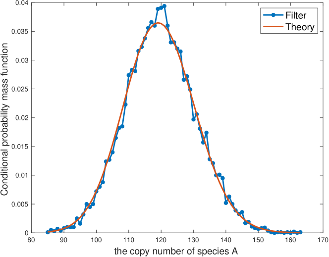
where Ξ»=∫0tc1​y​(t)​𝑑tπœ†superscriptsubscript0𝑑subscript𝑐1𝑦𝑑differential-d𝑑\lambda=\int_{0}^{t}c_{1}y(t)dt. With initial state #​A=0#𝐴0\#A=0 and #​S=5#𝑆5\#S=5, parameter values c=(1,5,1)𝑐151c=(1,5,1), and filter sample size Ns=10,000subscript𝑁𝑠10000N_{s}=10,000, we ran Algorithm 1, and Figure 1 shows the comparison between the conditional distribution computed by the filter with the exact conditional distribution.
Refer to caption
Figure 1: The conditional distribution of the number of A𝐴A at time T=20𝑇20T=20 conditioned on one observation of the entire trajectory of the copy number of S𝑆S on the interval [0,T]0𝑇[0,T], in the linear propensity example. The estimated conditional distribution Ο€^​(T,x)^πœ‹π‘‡π‘₯\hat{\pi}(T,x) and the exact theoretical conditional distribution π​(T,x)πœ‹π‘‡π‘₯\pi(T,x) are shown.

In order to estimate the CMTVE defined by (23), with same initial state, parameter values, final time T=20𝑇20T=20, filter sample size Ns=10,000subscript𝑁𝑠10000N_{s}=10,000, and the same observation trajectory, we ran 100 simulations of algorithm 1. From this we estimated CMTVE for the algorithm to be 0.04750.04750.0475 with a 95%percent9595\%confidence interval of [0.0461,0.0488]0.04610.0488[0.0461,0.0488].

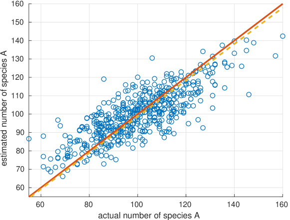
We also tested the filter’s performance on point estimation. To compare estimated state ℰ​(t)ℰ𝑑\mathcal{E}(t) with the actual state X​(t)𝑋𝑑X(t), as described in Section 4, we generated Nr=500subscriptπ‘π‘Ÿ500N_{r}=500 independent realizations of the system (X,Y)π‘‹π‘Œ(X,Y), and applied the filtering algorithm with filter sample size Ns=1000subscript𝑁𝑠1000N_{s}=1000 to get an estimate ℰ​(t)ℰ𝑑\mathcal{E}(t) for each of the realizations. Figure 2 shows a scatter plot of the values of ℰ​(T)ℰ𝑇\mathcal{E}(T) against X​(T)𝑋𝑇X(T). We note that ℰ​(T)ℰ𝑇\mathcal{E}(T) is a biased estimator whose bias is expected to approach zero as Nssubscript𝑁𝑠N_{s} tends to infinity. The fact that the regression line does not have slope 1 is due to this as well as due to finite sample size of Nrsubscriptπ‘π‘ŸN_{r}.

Refer to caption
Figure 2: Scatter plot of the point estimates ℰ​(T)ℰ𝑇\mathcal{E}(T) of the copy number of species A𝐴A at T=20𝑇20T=20 (based on the observation of species S𝑆S on the interval [0,T]0𝑇[0,T]) against the actual copy numbers X​(T)𝑋𝑇X(T) in the linear propensity example. In each trial, a realization of the system (X,Y)π‘‹π‘Œ(X,Y) was generated, and we computed the point estimates ℰ​(T)ℰ𝑇\mathcal{E}(T) of the copy number of species A𝐴A at time T𝑇T based on the trajectory of species S𝑆S. 500500500 independent trials were performed. The dashed yellow line is the regression line and solid red line is the line with slope 1. The bias is βˆ’0.28100.2810-0.2810 with a 95%percent9595\% confidence interval of [βˆ’1.20427,0.642256]1.204270.642256[-1.20427,0.642256] the estimated L2superscript𝐿2L^{2} error is 10.315910.315910.3159 with a 95%percent9595\% confidence interval of [9.58143,11.0014]9.5814311.0014[9.58143,11.0014].

Next, with the same system, we considered observing species A𝐴A rather than species S𝑆S. So Z​(t)=(X​(t),Y​(t))=(#​S​(t),#​A​(t))π‘π‘‘π‘‹π‘‘π‘Œπ‘‘#𝑆𝑑#𝐴𝑑Z(t)=(X(t),Y(t))=(\#S(t),\#A(t)). We kept the initial state and parameter values of c1subscript𝑐1c_{1} and c3subscript𝑐3c_{3} to be the same as before and performed a Bayesian estimation of parameter c2subscript𝑐2c_{2}. Thus we considered c2subscript𝑐2c_{2} as a random variable C2subscript𝐢2C_{2} with a uniform prior distribution on [4,6]46[4,6]. We randomly generated a sample of Nr=1000subscriptπ‘π‘Ÿ1000N_{r}=1000 values of C2subscript𝐢2C_{2} following uniform distribution [4,6]46[4,6] and generated one observation trajectory Yπ‘ŒY for each value of C2subscript𝐢2C_{2}. Then we applied Algorithm 5 to compute CΒ―2​(t)subscript¯𝐢2𝑑\bar{C}_{2}(t), the filter estimate of 𝔼​(C2|𝒴t)𝔼conditionalsubscript𝐢2subscript𝒴𝑑{\mathbb{E}}(C_{2}\,|\mathcal{Y}_{t}) (see (20). The result is shown in Figure 3.
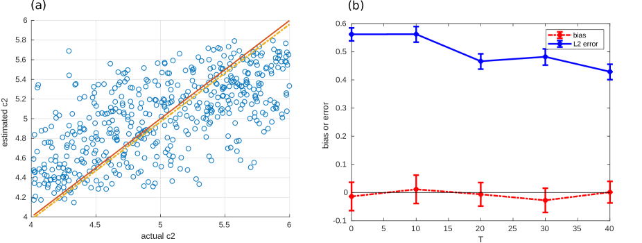
Refer to caption
Figure 3: (a) A scatter plot of CΒ―2​(40)subscript¯𝐢240\bar{C}_{2}(40), the estimated value of C2subscript𝐢2C_{2} (based on the observation of the copy number trajectory of species A𝐴A on the interval [0,40]040[0,40]), against the actual value of C2subscript𝐢2C_{2} in the linear propensity example. In each trial, we randomly generated a value of C2subscript𝐢2C_{2} following a uniform distribution on [4,6]46[4,6] and simulated the full system to generate an observation trajectory of species A𝐴A. Then we applied Algorithm 5 to compute CΒ―2​(40)subscript¯𝐢240\bar{C}_{2}(40), where a uniform (prior) distribution on the interval [4,6]46[4,6] was endowed. Filter sample size was Ns=1000subscript𝑁𝑠1000N_{s}=1000 and trial size Nr=500subscriptπ‘π‘Ÿ500N_{r}=500. (b) The bias 𝔼​[CΒ―2​(T)βˆ’C2]𝔼delimited-[]subscript¯𝐢2𝑇subscript𝐢2{\mathbb{E}}[\bar{C}_{2}(T)-C_{2}] as well as the L2superscript𝐿2L^{2} error 𝔼​[(CΒ―2​(T)βˆ’C2)2]1/2𝔼superscriptdelimited-[]superscriptsubscript¯𝐢2𝑇subscript𝐢2212{\mathbb{E}}[(\bar{C}_{2}(T)-C_{2})^{2}]^{1/2} (along with 95%percent9595\% confidence intervals) are plotted against T𝑇T. Decreasing L2superscript𝐿2L^{2} error with T𝑇T suggests that longer observations lead to better estimations.

5.2 Genetic Circuit Example

We consider a genetic transcription example [32] where a protein A𝐴A encoded by gene DAsubscript𝐷𝐴D_{A} could bind with its own gene promoter to enhance or suppress its transcription:

DA+Asubscript𝐷𝐴𝐴\displaystyle D_{A}+A ⟢c1DAβ€²,superscript⟢subscript𝑐1absentsuperscriptsubscript𝐷𝐴′\displaystyle\stackrel{{\scriptstyle c_{1}}}{{\longrightarrow}}D_{A}^{\prime}, (29)
DAβ€²superscriptsubscript𝐷𝐴′\displaystyle D_{A}^{\prime} ⟢c2DA+A,superscript⟢subscript𝑐2absentsubscript𝐷𝐴𝐴\displaystyle\stackrel{{\scriptstyle c_{2}}}{{\longrightarrow}}D_{A}+A,
DAsubscript𝐷𝐴\displaystyle D_{A} ⟢c3DA+A,superscript⟢subscript𝑐3absentsubscript𝐷𝐴𝐴\displaystyle\stackrel{{\scriptstyle c_{3}}}{{\longrightarrow}}D_{A}+A,
DAβ€²superscriptsubscript𝐷𝐴′\displaystyle D_{A}^{\prime} ⟢c4DAβ€²+A,superscript⟢subscript𝑐4absentsuperscriptsubscript𝐷𝐴′𝐴\displaystyle\stackrel{{\scriptstyle c_{4}}}{{\longrightarrow}}D_{A}^{\prime}+A,
A𝐴\displaystyle A ⟢c5βˆ….superscript⟢subscript𝑐5absent\displaystyle\stackrel{{\scriptstyle c_{5}}}{{\longrightarrow}}\varnothing.

Let Z​(t)=(#​DA​(t),#​DA′​(t),#​A​(t))𝑍𝑑#subscript𝐷𝐴𝑑#superscriptsubscript𝐷𝐴′𝑑#𝐴𝑑Z(t)=(\#D_{A}(t),\#D_{A}^{\prime}(t),\#A(t)) and suppose the propensity function has the mass action form a1​(z)=c1​z1​z3,a2​(z)=c2​z2,a3​(z)=c3​z1,a4​(z)=c4​z2,a5​(z)=c5​z3formulae-sequencesubscriptπ‘Ž1𝑧subscript𝑐1subscript𝑧1subscript𝑧3formulae-sequencesubscriptπ‘Ž2𝑧subscript𝑐2subscript𝑧2formulae-sequencesubscriptπ‘Ž3𝑧subscript𝑐3subscript𝑧1formulae-sequencesubscriptπ‘Ž4𝑧subscript𝑐4subscript𝑧2subscriptπ‘Ž5𝑧subscript𝑐5subscript𝑧3a_{1}(z)=c_{1}z_{1}z_{3},a_{2}(z)=c_{2}z_{2},a_{3}(z)=c_{3}z_{1},a_{4}(z)=c_{4}z_{2},a_{5}(z)=c_{5}z_{3}. Suppose we only observe the molecule counts of protein A𝐴A and would like to estimate the copy number of the naked form of gene promoter DAsubscript𝐷𝐴D_{A} and the bounded form of the gene promoter DAβ€²superscriptsubscript𝐷𝐴′D_{A}^{\prime}. We ran all numerical experiments with initial condition Z​(0)=(3,0,15)𝑍03015Z(0)=(3,0,15) and nominal parameter values c1=0.3,c2=3,c3=0.5,c4=0.2,c5=0.06formulae-sequencesubscript𝑐10.3formulae-sequencesubscript𝑐23formulae-sequencesubscript𝑐30.5formulae-sequencesubscript𝑐40.2subscript𝑐50.06c_{1}=0.3,c_{2}=3,c_{3}=0.5,c_{4}=0.2,c_{5}=0.06 and filter sample size Ns=10,000subscript𝑁𝑠10000N_{s}=10,000.

The estimation of the copy number of DAsubscript𝐷𝐴D_{A} at time t𝑑t based on observation of A𝐴A over [0,t]0𝑑[0,t] is shown in Figure 4.

Refer to caption
Figure 4: Estimation of copy number of DAsubscript𝐷𝐴D_{A} at time t𝑑t based on the observation of species A𝐴A over [0,t]0𝑑[0,t] (genetic circuit example). Estimates are shown at jump times of the observed species A𝐴A along with their 68%percent6868\% confidence intervals. Filter sample size used was Ns=10,000subscript𝑁𝑠10000N_{s}=10,000.

We estimated one parameter at a time while fixing the other parameters at their nominal values mentioned before. We chose a uniform distribution as the prior and the posterior conditional distributions corresponding to the same single observed trajectory at several snapshots in time are shown in Figure 5.
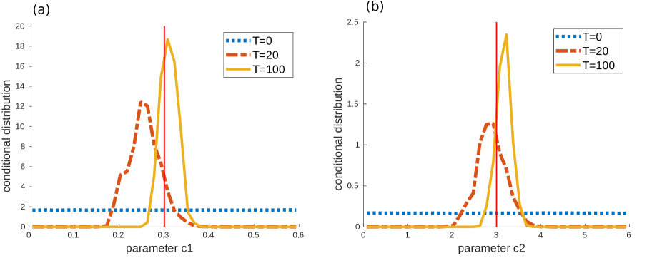
Refer to caption
Figure 5: The posterior conditional probability density function of parameters C1subscript𝐢1C_{1} and C2subscript𝐢2C_{2} based on one observed trajectory of A𝐴A on interval [0,T]0𝑇[0,T] in the genetic circuit example for T=0,20𝑇020T=0,20 and 100100100. The filter sample size was Ns=1,000,000subscript𝑁𝑠1000000N_{s}=1,000,000. T=0𝑇0T=0 is simply the uniform priors on C1subscript𝐢1C_{1} and C2subscript𝐢2C_{2}. The vertical lines show the true parameter values.

5.3 Genetic toggle switch

Consider the system of genetic toggle switch[16]

βˆ…\displaystyle\varnothing ⟢a1S1,superscript⟢subscriptπ‘Ž1absentsubscript𝑆1\displaystyle\stackrel{{\scriptstyle a_{1}}}{{\longrightarrow}}S_{1}, (30)
S1subscript𝑆1\displaystyle S_{1} ⟢a2βˆ…,superscript⟢subscriptπ‘Ž2absent\displaystyle\stackrel{{\scriptstyle a_{2}}}{{\longrightarrow}}\varnothing,
βˆ…\displaystyle\varnothing ⟢a3S2,superscript⟢subscriptπ‘Ž3absentsubscript𝑆2\displaystyle\stackrel{{\scriptstyle a_{3}}}{{\longrightarrow}}S_{2},
S2subscript𝑆2\displaystyle S_{2} ⟢a4βˆ….superscript⟢subscriptπ‘Ž4absent\displaystyle\stackrel{{\scriptstyle a_{4}}}{{\longrightarrow}}\varnothing.

Let Z​(t)=(X​(t),Y​(t))=(#​S1​(t),#​S2​(t))π‘π‘‘π‘‹π‘‘π‘Œπ‘‘#subscript𝑆1𝑑#subscript𝑆2𝑑Z(t)=(X(t),Y(t))=(\#S_{1}(t),\#S_{2}(t)) and suppose the propensity functions have the form a1​(z)=Ξ±11+yΞ²subscriptπ‘Ž1𝑧subscript𝛼11superscript𝑦𝛽a_{1}(z)=\frac{\alpha_{1}}{1+y^{\beta}}, a2​(z)=xsubscriptπ‘Ž2𝑧π‘₯a_{2}(z)=x, a3​(z)=Ξ±21+xΞ³subscriptπ‘Ž3𝑧subscript𝛼21superscriptπ‘₯𝛾a_{3}(z)=\frac{\alpha_{2}}{1+x^{\gamma}}, a4​(z)=ysubscriptπ‘Ž4𝑧𝑦a_{4}(z)=y. Suppose we only observe species S2subscript𝑆2S_{2} and we estimate the molecule counts of species S1subscript𝑆1S_{1}. We chose the initial condition Z​(0)=(0,0)𝑍000Z(0)=(0,0) and the nominal parameter values Ξ±1=50,Ξ±2=16,Ξ²=2.5,Ξ³=1formulae-sequencesubscript𝛼150formulae-sequencesubscript𝛼216formulae-sequence𝛽2.5𝛾1\alpha_{1}=50,\alpha_{2}=16,\beta=2.5,\gamma=1. The estimation of the molecular counts of species S1subscript𝑆1S_{1} right after each jump of #​S2​(t)#subscript𝑆2𝑑\#S_{2}(t) for a particular observed trajectory is shown in Figure 6 where a filter sample size of Ns=10,000subscript𝑁𝑠10000N_{s}=10,000 was used.

As in the genetic circuit example, we estimated one parameter at a time while fixing the other parameter at its nominal value mentioned before. We chose a uniform distribution as the prior and the posterior conditional distributions computed based on the same single observed trajectory at several snapshots in time are shown in Figure 7.

Figure 7 suggests that the inference of Ξ±2subscript𝛼2\alpha_{2} is much better than the inference of Ξ±1subscript𝛼1\alpha_{1}. To understand why, we note that in the toggle switch example, the trajectories of #​S1#subscript𝑆1\#S_{1} and #​S2#subscript𝑆2\#S_{2} exhibit a switching pattern that switches between two modes. In one mode, #​S1#subscript𝑆1\#S_{1} fluctuates around Ξ±1subscript𝛼1\alpha_{1} while #​S2#subscript𝑆2\#S_{2} is nearly zero, and in the other, #​S2#subscript𝑆2\#S_{2} fluctuates around Ξ±2subscript𝛼2\alpha_{2} while #​S1#subscript𝑆1\#S_{1} is nearly zero. The influence of Ξ±1subscript𝛼1\alpha_{1} on the behavior of S2subscript𝑆2S_{2} only enters indirectly, and we conjecture by affecting the switching frequency. If this were to be the case, one may need a long observation trajectory, perhaps beyond T=10,000𝑇10000T=10,000 to make a good estimate of Ξ±1subscript𝛼1\alpha_{1}. Longer time duration T𝑇T may require larger sample size Nssubscript𝑁𝑠N_{s} making the computations more tedious.

In order to test our hypothesis regarding the switching frequency, after some trial and error, we chose the parameter values Ξ±1=20subscript𝛼120\alpha_{1}=20 and Ξ±=9𝛼9\alpha=9 and kept the other two parameters the same. Figure 8 shows a comparison of trajectories of the system with the two different sets of parameters. We repeated the parameter inference experiment with this new choice of Ξ±1subscript𝛼1\alpha_{1} and Ξ±2subscript𝛼2\alpha_{2} and the results are shown in Figure 9 and show that Ξ±1subscript𝛼1\alpha_{1} is predicted better.

Refer to caption
Figure 6: Estimation of copy number of S1subscript𝑆1S_{1} at time t𝑑t in the genetic toggle switch example based on one observed trajectory of S2subscript𝑆2S_{2} over [0,t]0𝑑[0,t]. Estimates are shown at jump times of the observed species S2subscript𝑆2S_{2} along with their 68%percent6868\% confidence intervals. Filter sample size used was Ns=10,000subscript𝑁𝑠10000N_{s}=10,000.
Refer to caption
Figure 7: The posterior conditional probability density function of parameters Ξ±1subscript𝛼1\alpha_{1} (left) and Ξ±2subscript𝛼2\alpha_{2} (right) in the genetic toggle example based on the observation of the trajectory of #​S2#subscript𝑆2\#S_{2} over [0,T]0𝑇[0,T]. The nominal parameter values were Ξ±1=50,Ξ±2=16,Ξ²=2.5,Ξ³=1formulae-sequencesubscript𝛼150formulae-sequencesubscript𝛼216formulae-sequence𝛽2.5𝛾1\alpha_{1}=50,\alpha_{2}=16,\beta=2.5,\gamma=1. Estimates are shown at times T=0,20,100,1000𝑇0201001000T=0,20,100,1000 and 200020002000 on the left and T=0,20𝑇020T=0,20 and 100100100 on the right. The filter sample size was Ns=10,000subscript𝑁𝑠10000N_{s}=10,000. Note that T=0𝑇0T=0 corresponds to the uniform priors. Two different observation trajectories, one for the estimation of Ξ±1subscript𝛼1\alpha_{1} and the other for Ξ±2subscript𝛼2\alpha_{2} were used.
Refer to caption
Figure 8: Trajectories of the genetic toggle switch system under different parameters. The figure on the left has less frequent switching, which corresponds to Ξ±1=50,Ξ±2=16,Ξ²=2.5,Ξ³=1formulae-sequencesubscript𝛼150formulae-sequencesubscript𝛼216formulae-sequence𝛽2.5𝛾1\alpha_{1}=50,\alpha_{2}=16,\beta=2.5,\gamma=1, the figure on the right corresponds to Ξ±1=20,Ξ±2=9,Ξ²=2.5,Ξ³=1formulae-sequencesubscript𝛼120formulae-sequencesubscript𝛼29formulae-sequence𝛽2.5𝛾1\alpha_{1}=20,\alpha_{2}=9,\beta=2.5,\gamma=1.
Refer to caption
Figure 9: The posterior conditional probability density function of parameters Ξ±1subscript𝛼1\alpha_{1} (left) and Ξ±2subscript𝛼2\alpha_{2} (right) in the genetic toggle example based on the observation of the trajectory of #​S2#subscript𝑆2\#S_{2} over [0,T]0𝑇[0,T]. The nominal parameter values were Ξ±1=20,Ξ±2=9,Ξ²=2.5,Ξ³=1formulae-sequencesubscript𝛼120formulae-sequencesubscript𝛼29formulae-sequence𝛽2.5𝛾1\alpha_{1}=20,\alpha_{2}=9,\beta=2.5,\gamma=1. Estimates are shown at times T=0,20,100𝑇020100T=0,20,100 and 600600600 on the left and T=0,20𝑇020T=0,20 and 100100100 on the right. The filter sample size was Ns=100,0000subscript𝑁𝑠1000000N_{s}=100,0000. Note that T=0𝑇0T=0 corresponds to the uniform priors.

5.4 SEIR model

Consider the SEIR model for the spread of infectious diseases

S+I𝑆𝐼\displaystyle S+I ⟢βE+I,superscriptβŸΆπ›½absent𝐸𝐼\displaystyle\stackrel{{\scriptstyle\beta}}{{\longrightarrow}}E+I, (31)
E𝐸\displaystyle E ⟢κI,superscriptβŸΆπœ…absent𝐼\displaystyle\stackrel{{\scriptstyle\kappa}}{{\longrightarrow}}I,
I𝐼\displaystyle I ⟢γR.superscriptβŸΆπ›Ύabsent𝑅\displaystyle\stackrel{{\scriptstyle\gamma}}{{\longrightarrow}}R.

Let Z​(t)=(#​S​(t),#​E​(t),#​R​(t),#​I​(t))𝑍𝑑#𝑆𝑑#𝐸𝑑#𝑅𝑑#𝐼𝑑Z(t)=(\#S(t),\#E(t),\#R(t),\#I(t)) where S,E,I𝑆𝐸𝐼S,E,I and R𝑅R stand for susceptible, exposed, infected and recovered respectively. We assume that we could observe the infectious population I𝐼I exactly. The propensity functions aj​(β‹…)subscriptπ‘Žπ‘—β‹…a_{j}(\cdot) have the form a1​(z)=β​z1​z4/Nsubscriptπ‘Ž1𝑧𝛽subscript𝑧1subscript𝑧4𝑁a_{1}(z)=\beta z_{1}z_{4}/N, a2​(z)=κ​z2subscriptπ‘Ž2π‘§πœ…subscript𝑧2a_{2}(z)=\kappa z_{2}, a3​(z)=γ​z4subscriptπ‘Ž3𝑧𝛾subscript𝑧4a_{3}(z)=\gamma z_{4}, where N=z1+z2+z3+z4𝑁subscript𝑧1subscript𝑧2subscript𝑧3subscript𝑧4N=z_{1}+z_{2}+z_{3}+z_{4} is the total population. We ran all numerical experiments with initial condition Z​(0)=(s0,e0,r0,i0)=(500,20,0,5)𝑍0subscript𝑠0subscript𝑒0subscriptπ‘Ÿ0subscript𝑖05002005Z(0)=(s_{0},e_{0},r_{0},i_{0})=(500,20,0,5) and parameter values Ξ²=0.05,ΞΊ=0.2,Ξ³=0.05formulae-sequence𝛽0.05formulae-sequenceπœ…0.2𝛾0.05\beta=0.05,\kappa=0.2,\gamma=0.05.

The estimation of the susceptible and exposed population after each change of Z4​(t)=#​I​(t)subscript𝑍4𝑑#𝐼𝑑Z_{4}(t)=\#I(t) for a particular observed trajectory of I𝐼I is shown in Figure 10 where a filter sample size of Ns=10,000subscript𝑁𝑠10000N_{s}=10,000 was used. Figure 11 shows scatter plots corresponding to state estimation of susceptible and exposed number of individuals.

Keeping other parameters at their nominal values, we explored Bayesian inference of parameter ΞΊπœ…\kappa (the reciprocal of the incubation period) based on a uniform prior. The scatter plot of the parameter estimation of ΞΊπœ…\kappa based on Nr=1000subscriptπ‘π‘Ÿ1000N_{r}=1000 trials each with a filter sample size Ns=1000subscript𝑁𝑠1000N_{s}=1000 is in shown in Figure 12.

Refer to caption
Figure 10: Estimation of the susceptible population (left) and the exposed population (right) at time t𝑑t in the SEIR example given one trajectory of the infected population over [0,t]0𝑑[0,t]. Estimates are shown at times of observed new infections or recovery along with the 68%percent6868\% confidence intervals. Filter sample size used was Ns=10,000subscript𝑁𝑠10000N_{s}=10,000.
Refer to caption
Figure 11: Estimate of the susceptible (a) and exposed (b) population in SEIR example at time T=40𝑇40T=40 given observations of the infected population over [0,T]0𝑇[0,T]. The filter sample size was Ns=1000subscript𝑁𝑠1000N_{s}=1000, and trial size Nr=500subscriptπ‘π‘Ÿ500N_{r}=500. For the susceptible population, the bias is 0.01560.01560.0156 within a 95%percent9595\% confidence interval [βˆ’0.160955,0.192202]0.1609550.192202[-0.160955,0.192202] and L2subscript𝐿2L_{2} error is 1.97231.97231.9723 within [1.81684,2.11637]1.816842.11637[1.81684,2.11637]. For the exposed population, the bias is βˆ’0.01560.0156-0.0156 within a 95%percent9595\% confidence interval [βˆ’0.192202,0.160955]0.1922020.160955[-0.192202,0.160955] and L2subscript𝐿2L_{2} error is 1.97231.97231.9723 within [1.81684,2.11637]1.816842.11637[1.81684,2.11637].
Refer to caption
Figure 12: (a) A scatter plot of ΞΊ^​(T)^πœ…π‘‡\hat{\kappa}(T), the estimated value of ΞΊπœ…\kappa against the actual value of ΞΊπœ…\kappa. Here T=40𝑇40T=40. Filter sample size was Ns=1000subscript𝑁𝑠1000N_{s}=1000 and trial size Nr=500subscriptπ‘π‘Ÿ500N_{r}=500. (b) The the bias 𝔼​[ΞΊ^​(T)βˆ’ΞΊ]𝔼delimited-[]^πœ…π‘‡πœ…{\mathbb{E}}[\hat{\kappa}(T)-\kappa] as well as the L2superscript𝐿2L^{2} error 𝔼​[(ΞΊ^​(T)βˆ’ΞΊ)2]1/2𝔼superscriptdelimited-[]superscript^πœ…π‘‡πœ…212{\mathbb{E}}[(\hat{\kappa}(T)-\kappa)^{2}]^{1/2} (along with 95%percent9595\% confidence intervals) are plotted against T𝑇T.

Next we explore estimation of the state at a past time t0subscript𝑑0t_{0} based on observation up to a future time T𝑇T. That is 0≀t0≀T0subscript𝑑0𝑇0\leq t_{0}\leq T. The case of t0=0subscript𝑑00t_{0}=0 corresponds to the situation where the initial state itself is not known, but we only have a prior distribution for it. We assumed that the exposed population at initial time t=0𝑑0t=0 followed a binomial distribution, with parameters N=520𝑁520N=520 and p=0.04𝑝0.04p=0.04. Since #​I​(0)=5#𝐼05\#I(0)=5 and the total population is 525525525, this left us with 520520520 individuals. We assumed a probability p=0.04𝑝0.04p=0.04 of being exposed, which lead us to choose the binomial distribution. Algorithm 6 was used to estimate the conditional probability mass function

P​{X2​(t0)=x|Y​(s)=y​(s), 0≀s≀T}𝑃conditional-setsubscript𝑋2subscript𝑑0π‘₯formulae-sequenceπ‘Œπ‘ π‘¦π‘ β€‰0𝑠𝑇P\{X_{2}(t_{0})=x\,|\,Y(s)=y(s),\,0\leq s\leq T\}

for various t0subscript𝑑0t_{0} and T𝑇T. The results are shown in Figure 13.

Refer to caption
Figure 13: (a) Conditional distribution of the exposed population at the initial time X2​(0)|𝒴Tconditionalsubscript𝑋20subscript𝒴𝑇X_{2}(0)|\mathcal{Y}_{T} for T=0,20𝑇020T=0,20 and 404040. (b) Conditional distribution of the exposed population at an intermediate time X2​(10)|𝒴Tconditionalsubscript𝑋210subscript𝒴𝑇X_{2}(10)|\mathcal{Y}_{T} for T=10,20𝑇1020T=10,20 and 404040. Filter sample size was Ns=10,000subscript𝑁𝑠10000N_{s}=10,000. The prior of the initial distribution of the exposed population follows a binomial distribution B​(520,0.04)𝐡5200.04B(520,0.04).

5.5 Investigation of resampling

Here we investigate the strategies of resampling in our filter. In the numerical examples presented so far, we applied the offspring algorithm to resample right after each jump tksubscriptπ‘‘π‘˜t_{k}. Here we present the results of three different resampling strategies. One was to resample at each jump time tksubscriptπ‘‘π‘˜t_{k} as we did earlier. As an alternative, we applied an adaptive resampling method where resampling is applied at tksubscriptπ‘‘π‘˜t_{k} if more than 10 particles had zero weights or if the ratio of the maximum weight to the minimum nonzero weight was greater than 1000. The third alternative was not to resample at all. We note that, whenever resampling was not used, the weights were normalized instead so that the average weight was 1 right after any jump time tksubscriptπ‘‘π‘˜t_{k}.

Table 1 shows the L2superscript𝐿2L^{2} error as well as the bias in estimating the conditional mean of the state or a parameter along with the 95%percent9595\% confidence intervals, for the various examples considered earlier. The results are for state estimation unless a parameter is mentioned in the first column. The entrees NaN indicate numerical issues in MATLAB mainly due to the fact that all weights became either zero or infinity within numerical precision. These results show that the three approaches yield more or less the same accuracy (the estimated errors are within the confidence intervals of each other) except in the case of the genetic circuit example where serious numerical issues manifest without resampling. We suspect that in the other examples, if final time T𝑇T is increased, the need for resampling will become evident.

Table 1: The bias and error of estimation of the states or parameters when different resampling schemes were applied.
System Method L2superscript𝐿2L^{2} error Confidence interval bias Condidence interval
linear propensity each jump 9.74709.74709.7470 [9.0677,10.3819]9.067710.3819[9.0677,10.3819] βˆ’0.33460.3346-0.3346 [βˆ’1.2068,0.5375]1.20680.5375[-1.2068,0.5375]
linear propensity adaptive (0%)percent0(0\%) 10.021610.021610.0216 [9.3373,10.6621]9.337310.6621[9.3373,10.6621] βˆ’0.06990.0699-0.0699 [βˆ’0.9671,0.8273]0.96710.8273[-0.9671,0.8273]
linear propensity never 10.078310.078310.0783 [9.4464,10.6728]9.446410.6728[9.4464,10.6728] βˆ’0.49100.4910-0.4910 [βˆ’1.3922,0.4103]1.39220.4103[-1.3922,0.4103]
genetic circuit each jump 0.56380.56380.5638 [0.5241,0.6009]0.52410.6009[0.5241,0.6009] 0.01000.01000.0100 [βˆ’0.0405,0.0604]0.04050.0604[-0.0405,0.0604]
genetic circuit adaptive (75.85%)percent75.85(75.85\%) 0.54560.54560.5456 [0.5066,0.5820]0.50660.5820[0.5066,0.5820] βˆ’0.00850.0085-0.0085 [βˆ’0.0574,0.0403]0.05740.0403[-0.0574,0.0403]
genetic circuit never NaN NaN NaN NaN
genetic toggle each jump 5.50835.50835.5083 [5.0655,5.9181]5.06555.9181[5.0655,5.9181] 0.37010.37010.3701 [βˆ’0.1219,0.8622]0.12190.8622[-0.1219,0.8622]
genetic toggle adaptive (2.20%)percent2.20(2.20\%) 5.53075.53075.5307 [5.0344,5.9860]5.03445.9860[5.0344,5.9860] 0.24060.24060.2406 [βˆ’0.2541,0.7353]0.25410.7353[-0.2541,0.7353]
genetic toggle never 5.41755.41755.4175 [4.9015,5.8886]4.90155.8886[4.9015,5.8886] βˆ’0.81340.8134-0.8134 [βˆ’1.2930,βˆ’0.3339]1.29300.3339[-1.2930,-0.3339]
SEIR each jump 2.08532.08532.0853 [1.9323,2.2279]1.93232.2279[1.9323,2.2279] βˆ’0.01760.0176-0.0176 [βˆ’0.2043,0.1691]0.20430.1691[-0.2043,0.1691]
SEIR adaptive (9.91%)percent9.91(9.91\%) 2.37262.37262.3726 [2.2102,2.5245]2.21022.5245[2.2102,2.5245] 0.12380.12380.1238 [βˆ’0.0884,0.3359]0.08840.3359[-0.0884,0.3359]
SEIR never 2.08232.08232.0823 [1.9572,2.2003]1.95722.2003[1.9572,2.2003] βˆ’0.00290.0029-0.0029 [βˆ’0.1893,0.1835]0.18930.1835[-0.1893,0.1835]
linear propensity c2subscript𝑐2c_{2} each jump 0.40990.40990.4099 [0.3850,0.4334]0.38500.4334[0.3850,0.4334] 0.02330.02330.0233 [βˆ’0.0134,0.0599]0.01340.0599[-0.0134,0.0599]
linear propensity c2subscript𝑐2c_{2} adaptive (23.00%)percent23.00(23.00\%) 0.42370.42370.4237 [0.3977,0.4481]0.39770.4481[0.3977,0.4481] βˆ’0.02950.0295-0.0295 [βˆ’0.0674,0.0083]0.06740.0083[-0.0674,0.0083]
linear propensity c2subscript𝑐2c_{2} never 0.53800.53800.5380 [0.5022,0.5716]0.50220.5716[0.5022,0.5716] 0.06280.06280.0628 [0.0149,0.1106]0.01490.1106[0.0149,0.1106]
SEIR ΞΊπœ…\kappa each jump 0.03770.03770.0377 [0.0354,0.0398]0.03540.0398[0.0354,0.0398] 0.00020.00020.0002 [βˆ’0.003,0.004]0.0030.004[-0.003,0.004]
SEIR ΞΊπœ…\kappa adaptive (20.61%)percent20.61(20.61\%) 0.03510.03510.0351 [0.0329,0.0372]0.03290.0372[0.0329,0.0372] βˆ’0.0030.003-0.003 [βˆ’0.004,0.0028]0.0040.0028[-0.004,0.0028]
SEIR ΞΊπœ…\kappa never 0.03710.03710.0371 [0.0343,0.0396]0.03430.0396[0.0343,0.0396] βˆ’0.00640.0064-0.0064 [βˆ’0.0097,βˆ’0.003]0.00970.003[-0.0097,-0.003]

6 Conclusions and future work

We presented a novel filtering algorithm to compute the conditional probability mass function

π​(t,x)=P​{X​(t)=x|Y​(s)=y​(s),0≀s≀t},πœ‹π‘‘π‘₯𝑃conditional-set𝑋𝑑π‘₯formulae-sequenceπ‘Œπ‘ π‘¦π‘ 0𝑠𝑑\pi(t,x)=P\{X(t)=x\,|\,Y(s)=y(s),0\leq s\leq t\},

in the context of reaction networks. Here Y​(t)=y​(t)π‘Œπ‘‘π‘¦π‘‘Y(t)=y(t) is the vector copy number of a subset of species that are assumed to be observed exactly in continuous time and X​(t)𝑋𝑑X(t) is the vector copy number of the remaining unobserved species. We also showed how this algorithm can be adapted for the purposes of Bayesian parameter estimation based on exact partial state observation. Furthermore, we also showed how the state X​(t0)𝑋subscript𝑑0X(t_{0}) at time t0subscript𝑑0t_{0} can be estimated based on observations up to a later time T𝑇T where 0≀t0≀T0subscript𝑑0𝑇0\leq t_{0}\leq T.

The filtering algorithm involves a weighted Monte Carlo method and a resampling strategy needs to be employed. We explored some possibilities for resampling at the observed jump times tksubscriptπ‘‘π‘˜t_{k}. Our investigations in this regards were numerical and based on relatively simple examples, and hence not exhaustive. An investigation of adaptive resampling based on some theoretical analysis is the subject of future work.

While we presented an intuitive derivation of the filtering equations, our derivation is not mathematically rigorous. [10] provides a rigorous derivation in the context of finite state Markov processes which in the case of reaction networks correspond to systems where species conservation relations limit the species counts to be bounded. A rigorous derivation is certainly possible for the case of unbounded species copy numbers provided certain integrability or moment bound conditions hold. In this context conditions in Refs.Β  [30, 24, 12] will be relevant.

As is well known, many intracellular reaction networks may have some species in greater abundance and a discrete state model can be tedious to simulate one event at a time. Tau-leap methods [20] as well as model reduction approaches have been proposed for efficient simulation of such systems. See [21] and references therein for several methods as well as [5, 28, 25, 15, 29, 2, 31] for rigorous mathematical analysis of methods. These same considerations could be applied to the filtering method proposed here to develop reduced order models and tau-leap simulations.

Our assumption of exact (noiseless) observation of some species may appear unrealistic. However, as mentioned in the introduction, most observation noise may be modeled via extra reactions and extra species such as photons. If the photon counts are very large, the same considerations of reduced order models or tau-leaping mentioned above apply. Less realistic is the assumption of continuous in time observations. In reality, observations are recorded in discrete time snapshots. If the frequency of the snapshots is very high, then the theory of continuous in time observations provides a good approximation. If the frequency is low, then this is not the case. Future work will involve the case where observations of some species are made at certain time snapshots as well as the limiting behavior as the time snapshots increase in frequency. Either way, the theory and the algorithm discussed in this paper provides a baseline for the exploration of observations at discrete time snapshots.

Acknowledgments: We thank Ankit Gupta for introducing us to the rich and subtle topic of stochastic filtering.

Appendix A Derivation of the evolution equations for π​(t,x)πœ‹π‘‘π‘₯\pi(t,x)

We note that [10] provides a rigorous derivation of the evolution equation for the conditional probability π​(t,z)πœ‹π‘‘π‘§\pi(t,z) when the state space is finite and the exact observation is of the form y=h​(z)π‘¦β„Žπ‘§y=h(z) where hβ„Žh is a function of the state space. The derivation in Ref.Β  [10] may not be easily accessible to applied scientists who may not be familiar with the language of stochastic analysis. Moreover, our filtering equations (while in agreement with Ref.Β  [10]) are somewhat simpler in appearance since in our case hβ„Žh corresponds to the projection onto the last n2subscript𝑛2n_{2} components of the state and also due to the structure of the reaction network. The derivation shown here is more intuitive to follow (at the expense of some rigor) and results in equations consistent with [10]. Moreover, we shall not make the assumption that the state space is finite. We believe that the rigorous derivation in Ref.Β  [10] can be extended to infinite state space under reasonable assumptions, but such an endeavor is beyond the scope of this paper.

We start with a discretization of the time interval [0,∞)0[0,\infty) by a mesh

{ℓ​h|β„“=0,1,…}conditional-setβ„“β„Žβ„“01…\{\ell h\,|\ell=0,1,\dots\}

of spacing hβ„Žh. We consider (X​(ℓ​h),Y​(ℓ​h))π‘‹β„“β„Žπ‘Œβ„“β„Ž(X(\ell h),Y(\ell h)) as a discrete time Markov chain. If the observed trajectory of Y​(t)π‘Œπ‘‘Y(t) is given by y​(t)𝑦𝑑y(t), then the observations on the mesh points will be given by

yΒ―β„“=y​(ℓ​h),β„“=0,1,…formulae-sequencesubscriptΒ―π‘¦β„“π‘¦β„“β„Žβ„“01…\bar{y}_{\ell}=y(\ell h),\quad\ell=0,1,\dots

We may use the filtering equations for a partially observed discrete time Markov chain derived in [14]. For the discrete time Markov chain (X​(ℓ​h),Y​(ℓ​h))π‘‹β„“β„Žπ‘Œβ„“β„Ž(X(\ell h),Y(\ell h)) (for β„“=0,1,…ℓ01…\ell=0,1,\dots) where Yπ‘ŒY is observed exactly, the conditional probability

Ο€β„“(x)=P(X(β„“h)=x|Y(jh)=yΒ―jj=0,…,n),\pi_{\ell}(x)=P(X(\ell h)=x\,|\,Y(jh)=\bar{y}_{j}\,j=0,\dots,n),

is shown in [14] to satisfy

πℓ​(xβ€²)=βˆ‘xκ​((x,yΒ―β„“βˆ’1),(xβ€²,yΒ―β„“))β€‹Ο€β„“βˆ’1​(x)βˆ‘xβ„“βˆ‘xβ„“βˆ’1κ​((xβ„“βˆ’1,yΒ―β„“βˆ’1),(xβ„“,yΒ―β„“))β€‹Ο€β„“βˆ’1​(xβ„“βˆ’1),subscriptπœ‹β„“superscriptπ‘₯β€²subscriptπ‘₯πœ…π‘₯subscript¯𝑦ℓ1superscriptπ‘₯β€²subscript¯𝑦ℓsubscriptπœ‹β„“1π‘₯subscriptsubscriptπ‘₯β„“subscriptsubscriptπ‘₯β„“1πœ…subscriptπ‘₯β„“1subscript¯𝑦ℓ1subscriptπ‘₯β„“subscript¯𝑦ℓsubscriptπœ‹β„“1subscriptπ‘₯β„“1\pi_{\ell}(x^{\prime})=\frac{\sum_{x}\kappa((x,\bar{y}_{\ell-1}),(x^{\prime},\bar{y}_{\ell}))\pi_{\ell-1}(x)}{\sum_{x_{\ell}}\sum_{x_{\ell-1}}\kappa((x_{\ell-1},\bar{y}_{\ell-1}),(x_{\ell},\bar{y}_{\ell}))\pi_{\ell-1}(x_{\ell-1})}, (32)

where

ΞΊ((x,y),(xβ€²,yβ€²))=P(X(β„“h)=xβ€²,Y(β„“h)=yβ€²|X((β„“βˆ’1)h)=x,Y((β„“βˆ’1)h)=y).\kappa((x,y),(x^{\prime},y^{\prime}))=P(X(\ell h)=x^{\prime},Y(\ell h)=y^{\prime}\,|\,X((\ell-1)h)=x,Y((\ell-1)h)=y).

From the infinitesimal characteristics of continuous time Markov chains, as hβ„Žh approaches 0+limit-from00+,

κ​((x,y),(xβ€²,yβ€²))πœ…π‘₯𝑦superscriptπ‘₯β€²superscript𝑦′\displaystyle\kappa((x,y),(x^{\prime},y^{\prime})) =aj​(x,y)​h+o​(h)(xβ€²,yβ€²)=(x,y)+Ξ½j,formulae-sequenceabsentsubscriptπ‘Žπ‘—π‘₯π‘¦β„Žπ‘œβ„Žsuperscriptπ‘₯β€²superscript𝑦′π‘₯𝑦subscriptπœˆπ‘—\displaystyle=a_{j}(x,y)h+o(h)\quad(x^{\prime},y^{\prime})=(x,y)+\nu_{j}, (33)
κ​((x,y),(x,y))πœ…π‘₯𝑦π‘₯𝑦\displaystyle\kappa((x,y),(x,y)) =1βˆ’hβ€‹βˆ‘j=1maj​(x,y)+o​(h),absent1β„Žsuperscriptsubscript𝑗1π‘šsubscriptπ‘Žπ‘—π‘₯π‘¦π‘œβ„Ž\displaystyle=1-h\sum_{j=1}^{m}a_{j}(x,y)+o(h),
κ​((x,y),(xβ€²,yβ€²))πœ…π‘₯𝑦superscriptπ‘₯β€²superscript𝑦′\displaystyle\kappa((x,y),(x^{\prime},y^{\prime})) =o​(h)Β otherwise.absentπ‘œβ„ŽΒ otherwise.\displaystyle=o(h)\quad\text{ otherwise.}

Let’s consider two adjacent mesh points t𝑑t and t+hπ‘‘β„Žt+h. There are two possibilities; there are no jumps of y𝑦y on the interval (t,t+h]π‘‘π‘‘β„Ž(t,t+h] or there are jumps. Again from the infinitesimal characteristics of continuous time Markov chains, as hβ„Žh approaches 0+limit-from00+, there is either no jump or one jump during (t,t+h]π‘‘π‘‘β„Ž(t,t+h]. We approximate π​(t,x)πœ‹π‘‘π‘₯\pi(t,x) by Ο€β„“βˆ’1​(x)subscriptπœ‹β„“1π‘₯\pi_{\ell-1}(x) and π​(t+h,x)πœ‹π‘‘β„Žπ‘₯\pi(t+h,x) by πℓ​(x)subscriptπœ‹β„“π‘₯\pi_{\ell}(x). For the case when there is no jump during (t,t+h]π‘‘π‘‘β„Ž(t,t+h], if we suppose tk≀t<t+h<tk+1subscriptπ‘‘π‘˜π‘‘π‘‘β„Žsubscriptπ‘‘π‘˜1t_{k}\leq t<t+h<t_{k+1}, then

yΒ―β„“=yΒ―β„“βˆ’1=y​(tk).subscript¯𝑦ℓsubscript¯𝑦ℓ1𝑦subscriptπ‘‘π‘˜\bar{y}_{\ell}=\bar{y}_{\ell-1}=y(t_{k}).

Using (32) and (33), we obtain π​(t+h,x)πœ‹π‘‘β„Žπ‘₯\pi(t+h,x) as a ratio where the numerator is

βˆ‘jβˆˆπ’°Ο€β€‹(t,xβˆ’Ξ½jβ€²)​aj​(xβˆ’Ξ½jβ€²,y​(tk))​h+π​(t,x)βˆ’Ο€β€‹(t,x)β€‹βˆ‘j=1maj​(x,y​(tk))​h+o​(h)subscriptπ‘—π’°πœ‹π‘‘π‘₯superscriptsubscriptπœˆπ‘—β€²subscriptπ‘Žπ‘—π‘₯superscriptsubscriptπœˆπ‘—β€²π‘¦subscriptπ‘‘π‘˜β„Žπœ‹π‘‘π‘₯πœ‹π‘‘π‘₯superscriptsubscript𝑗1π‘šsubscriptπ‘Žπ‘—π‘₯𝑦subscriptπ‘‘π‘˜β„Žπ‘œβ„Ž\sum_{j\in\mathcal{U}}\pi(t,x-\nu_{j}^{\prime})a_{j}(x-\nu_{j}^{\prime},y(t_{k}))h+\pi(t,x)-\pi(t,x)\sum_{j=1}^{m}a_{j}(x,y(t_{k}))h+o(h)

and the denominator is

βˆ‘x~(1βˆ’βˆ‘j∈π’ͺaj​(x~,y​(tk))​h)​π​(t,x~)+o​(h).subscript~π‘₯1subscript𝑗π’ͺsubscriptπ‘Žπ‘—~π‘₯𝑦subscriptπ‘‘π‘˜β„Žπœ‹π‘‘~π‘₯π‘œβ„Ž\sum_{\tilde{x}}\left(1-\sum_{j\in\mathcal{O}}a_{j}(\tilde{x},y(t_{k}))h\right)\pi(t,\tilde{x})+o(h).

From the above, we may obtain an expression for (π​(t+h,x)βˆ’Ο€β€‹(t,x))/hπœ‹π‘‘β„Žπ‘₯πœ‹π‘‘π‘₯β„Ž(\pi(t+h,x)-\pi(t,x))/h which upon taking limit as hβ†’0+β†’β„Žlimit-from0h\to 0+ yields (4). The second case is when t<tk<t+h𝑑subscriptπ‘‘π‘˜π‘‘β„Žt<t_{k}<t+h and in this case

yΒ―β„“βˆ’1=y​(tkβˆ’1)β‰ y​(tk)=yΒ―β„“.subscript¯𝑦ℓ1𝑦subscriptπ‘‘π‘˜1𝑦subscriptπ‘‘π‘˜subscript¯𝑦ℓ\bar{y}_{\ell-1}=y(t_{k-1})\neq y(t_{k})=\bar{y}_{\ell}.

Using (32) and (33), we obtain

π​(t+h,x)=βˆ‘l∈π’ͺkal​(xβˆ’Ξ½lβ€²,y​(tkβˆ’1))​π​(t,xβˆ’Ξ½lβ€²)​h+o​(h)βˆ‘x~βˆ‘l∈π’ͺkal​(x~βˆ’Ξ½lβ€²,y​(tkβˆ’1))​π​(t,x~)​h+o​(h).πœ‹π‘‘β„Žπ‘₯subscript𝑙subscriptπ’ͺπ‘˜subscriptπ‘Žπ‘™π‘₯subscriptsuperscriptπœˆβ€²π‘™π‘¦subscriptπ‘‘π‘˜1πœ‹π‘‘π‘₯subscriptsuperscriptπœˆβ€²π‘™β„Žπ‘œβ„Žsubscript~π‘₯subscript𝑙subscriptπ’ͺπ‘˜subscriptπ‘Žπ‘™~π‘₯subscriptsuperscriptπœˆβ€²π‘™π‘¦subscriptπ‘‘π‘˜1πœ‹π‘‘~π‘₯β„Žπ‘œβ„Ž\pi(t+h,x)=\frac{\sum_{l\in\mathcal{O}_{k}}a_{l}(x-\nu^{\prime}_{l},y(t_{k-1}))\,\pi(t,x-\nu^{\prime}_{l})\,h+o(h)}{\sum_{\tilde{x}}\sum_{l\in\mathcal{O}_{k}}a_{l}(\tilde{x}-\nu^{\prime}_{l},y(t_{k-1}))\,\pi(t,\tilde{x})\,h+o(h)}.

Noting that π​(t+h,x)→π​(tk,x)β†’πœ‹π‘‘β„Žπ‘₯πœ‹subscriptπ‘‘π‘˜π‘₯\pi(t+h,x)\to\pi(t_{k},x) and π​(t,x)→π​(tkβˆ’,x)β†’πœ‹π‘‘π‘₯πœ‹limit-fromsubscriptπ‘‘π‘˜π‘₯\pi(t,x)\to\pi(t_{k}-,x) as hβ†’0+β†’β„Žlimit-from0h\to 0+, we obtain (5).

We note that for a rigorous treatment one needs to use the language of measure theory, since unlike in the discrete time Markov chain case, in the continuous time case we are conditioning on a zero probability event of observing Y​(s)=y​(s)π‘Œπ‘ π‘¦π‘ Y(s)=y(s) for 0≀s≀t0𝑠𝑑0\leq s\leq t. Moreover, a rigorous and mathematically β€œcleaner” treatment involves working with the integral representation of the differential equation with jumps. The derivation provided here, we hope, provides the β€œessence” of the idea.

Appendix B Unnormalized and normalized filtering equations

We show that if ρ​(t,x)πœŒπ‘‘π‘₯\rho(t,x) satisfies the unnormalized filtering equations, then π​(t,x)=ρ​(t,x)/βˆ‘x~ρ​(t,x~)πœ‹π‘‘π‘₯πœŒπ‘‘π‘₯subscript~π‘₯πœŒπ‘‘~π‘₯\pi(t,x)=\rho(t,x)/\sum_{\tilde{x}}{\rho}(t,\tilde{x}). We assume the existence and uniqueness of solutions of both the unnormalized and normalized filtering equations.

To that end, suppose ρ𝜌\rho solves the unnormalized filtering equations (8) and (9), and let Ο€~​(t,x)=ρ​(t,x)/βˆ‘x~ρ​(t,x~)~πœ‹π‘‘π‘₯πœŒπ‘‘π‘₯subscript~π‘₯πœŒπ‘‘~π‘₯\tilde{\pi}(t,x)=\rho(t,x)/\sum_{\tilde{x}}{\rho}(t,\tilde{x}). It is adequate to show that Ο€~​(t,x)~πœ‹π‘‘π‘₯\tilde{\pi}(t,x) satisfies the filtering equations (4) and (5).

In between jump times, that is, for tk≀t<tk+1subscriptπ‘‘π‘˜π‘‘subscriptπ‘‘π‘˜1t_{k}\leq t<t_{k+1}, ρ𝜌\rho satisfies

ρ′​(t,x)superscriptπœŒβ€²π‘‘π‘₯\displaystyle\rho^{\prime}(t,x) =βˆ‘jβˆˆπ’°Οβ€‹(t,xβˆ’Ξ½jβ€²)​aj​(xβˆ’Ξ½jβ€²,y​(tk))βˆ’βˆ‘jβˆˆπ’°Οβ€‹(t,x)​aj​(x,y​(tk))absentsubscriptπ‘—π’°πœŒπ‘‘π‘₯superscriptsubscriptπœˆπ‘—β€²subscriptπ‘Žπ‘—π‘₯superscriptsubscriptπœˆπ‘—β€²π‘¦subscriptπ‘‘π‘˜subscriptπ‘—π’°πœŒπ‘‘π‘₯subscriptπ‘Žπ‘—π‘₯𝑦subscriptπ‘‘π‘˜\displaystyle=\sum_{j\in\mathcal{U}}\rho(t,x-\nu_{j}^{\prime})\,a_{j}(x-\nu_{j}^{\prime},y(t_{k}))-\sum_{j\in\mathcal{U}}\rho(t,x)\,a_{j}(x,y(t_{k}))
βˆ’Οβ€‹(t,x)​aπ’ͺ​(x,y​(tk))βˆ€xβˆˆβ„€+n1.πœŒπ‘‘π‘₯superscriptπ‘Žπ’ͺπ‘₯𝑦subscriptπ‘‘π‘˜for-allπ‘₯superscriptsubscriptβ„€subscript𝑛1\displaystyle-\rho(t,x)\,a^{\mathcal{O}}(x,y(t_{k}))\quad\forall x\in{\mathbb{Z}}_{+}^{n_{1}}.

Then

Ο€~′​(t,x)=ρ′​(t,x)βˆ‘x~ρ​(t,x~)βˆ’Οβ€‹(t,x)β€‹βˆ‘x~ρ′​(t,x~)(βˆ‘x~ρ​(t,x~))2.superscript~πœ‹β€²π‘‘π‘₯superscriptπœŒβ€²π‘‘π‘₯subscript~π‘₯πœŒπ‘‘~π‘₯πœŒπ‘‘π‘₯subscript~π‘₯superscriptπœŒβ€²π‘‘~π‘₯superscriptsubscript~π‘₯πœŒπ‘‘~π‘₯2\begin{split}\tilde{\pi}^{\prime}(t,x)=\frac{\rho^{\prime}(t,x)}{\sum_{\tilde{x}}{\rho}(t,\tilde{x})}-\rho(t,x)\frac{\sum_{\tilde{x}}{\rho^{\prime}}(t,\tilde{x})}{(\sum_{\tilde{x}}{\rho}(t,\tilde{x}))^{2}}.\end{split}

The first term may be written as

ρ′​(t,x)βˆ‘x~ρ​(t,x~)=βˆ‘jβˆˆπ’°Ο€~​(t,xβˆ’Ξ½jβ€²)​aj​(xβˆ’Ξ½jβ€²,y​(tk))βˆ’βˆ‘jβˆˆπ’°Ο€~​(t,x)​aj​(x,y​(tk))βˆ’Ο€~​(t,x)​aπ’ͺ​(x,y​(tk)).superscriptπœŒβ€²π‘‘π‘₯subscript~π‘₯πœŒπ‘‘~π‘₯subscript𝑗𝒰~πœ‹π‘‘π‘₯superscriptsubscriptπœˆπ‘—β€²subscriptπ‘Žπ‘—π‘₯superscriptsubscriptπœˆπ‘—β€²π‘¦subscriptπ‘‘π‘˜subscript𝑗𝒰~πœ‹π‘‘π‘₯subscriptπ‘Žπ‘—π‘₯𝑦subscriptπ‘‘π‘˜~πœ‹π‘‘π‘₯superscriptπ‘Žπ’ͺπ‘₯𝑦subscriptπ‘‘π‘˜\frac{\rho^{\prime}(t,x)}{\sum_{\tilde{x}}{\rho}(t,\tilde{x})}=\sum_{j\in\mathcal{U}}\tilde{\pi}(t,x-\nu_{j}^{\prime})\,a_{j}(x-\nu_{j}^{\prime},y(t_{k}))-\sum_{j\in\mathcal{U}}\tilde{\pi}(t,x)\,a_{j}(x,y(t_{k}))-\tilde{\pi}(t,x)\,a^{\mathcal{O}}(x,y(t_{k})).

The second term can be written as

ρ​(t,x)β€‹βˆ‘x~ρ′​(t,x~)(βˆ‘x~ρ​(t,x~))2=π​(t,x)β€‹βˆ‘x~ρ′​(t,x~)βˆ‘x~ρ​(t,x~)πœŒπ‘‘π‘₯subscript~π‘₯superscriptπœŒβ€²π‘‘~π‘₯superscriptsubscript~π‘₯πœŒπ‘‘~π‘₯2πœ‹π‘‘π‘₯subscript~π‘₯superscriptπœŒβ€²π‘‘~π‘₯subscript~π‘₯πœŒπ‘‘~π‘₯\rho(t,x)\frac{\sum_{\tilde{x}}{\rho^{\prime}}(t,\tilde{x})}{(\sum_{\tilde{x}}{\rho}(t,\tilde{x}))^{2}}=\pi(t,x)\frac{\sum_{\tilde{x}}{\rho^{\prime}}(t,\tilde{x})}{\sum_{\tilde{x}}{\rho}(t,\tilde{x})}

Note that βˆ‘x~(βˆ‘jβˆˆπ’°Οβ€‹(t,x~βˆ’Ξ½jβ€²)​aj​(x~βˆ’Ξ½jβ€²,y​(tk))βˆ’βˆ‘jβˆˆπ’°Οβ€‹(t,x~)​aj​(x~,y​(tk)))=0subscript~π‘₯subscriptπ‘—π’°πœŒπ‘‘~π‘₯superscriptsubscriptπœˆπ‘—β€²subscriptπ‘Žπ‘—~π‘₯superscriptsubscriptπœˆπ‘—β€²π‘¦subscriptπ‘‘π‘˜subscriptπ‘—π’°πœŒπ‘‘~π‘₯subscriptπ‘Žπ‘—~π‘₯𝑦subscriptπ‘‘π‘˜0\sum_{\tilde{x}}\left(\sum_{j\in\mathcal{U}}\rho(t,\tilde{x}-\nu_{j}^{\prime})\,a_{j}(\tilde{x}-\nu_{j}^{\prime},y(t_{k}))-\sum_{j\in\mathcal{U}}\rho(t,\tilde{x})\,a_{j}(\tilde{x},y(t_{k}))\right)=0, and hence

βˆ‘x~ρ′​(t,x~)=βˆ‘x~(βˆ‘jβˆˆπ’°Οβ€‹(t,x~βˆ’Ξ½jβ€²)​aj​(x~βˆ’Ξ½jβ€²,y​(tk))βˆ’βˆ‘jβˆˆπ’°Οβ€‹(t,x~)​aj​(x~,y​(tk))βˆ’Οβ€‹(t,x~)​aπ’ͺ​(x~,y​(tk)))=βˆ’βˆ‘x~ρ​(t,x~)​aπ’ͺ​(x~,y​(tk))subscript~π‘₯superscriptπœŒβ€²π‘‘~π‘₯subscript~π‘₯subscriptπ‘—π’°πœŒπ‘‘~π‘₯superscriptsubscriptπœˆπ‘—β€²subscriptπ‘Žπ‘—~π‘₯superscriptsubscriptπœˆπ‘—β€²π‘¦subscriptπ‘‘π‘˜subscriptπ‘—π’°πœŒπ‘‘~π‘₯subscriptπ‘Žπ‘—~π‘₯𝑦subscriptπ‘‘π‘˜πœŒπ‘‘~π‘₯superscriptπ‘Žπ’ͺ~π‘₯𝑦subscriptπ‘‘π‘˜subscript~π‘₯πœŒπ‘‘~π‘₯superscriptπ‘Žπ’ͺ~π‘₯𝑦subscriptπ‘‘π‘˜\begin{split}\sum_{\tilde{x}}{\rho^{\prime}}(t,\tilde{x})&=\sum_{\tilde{x}}\left(\sum_{j\in\mathcal{U}}\rho(t,\tilde{x}-\nu_{j}^{\prime})\,a_{j}(\tilde{x}-\nu_{j}^{\prime},y(t_{k}))-\sum_{j\in\mathcal{U}}\rho(t,\tilde{x})\,a_{j}(\tilde{x},y(t_{k}))-\rho(t,\tilde{x})\,a^{\mathcal{O}}(\tilde{x},y(t_{k}))\right)\\ &=-\sum_{\tilde{x}}\rho(t,\tilde{x})\,a^{\mathcal{O}}(\tilde{x},y(t_{k}))\end{split}

Hence Ο€~~πœ‹\tilde{\pi} satisfies (4).

For k=1,2,β€¦π‘˜12…k=1,2,\dots at jump times tksubscriptπ‘‘π‘˜t_{k}, ρ​(t,x)πœŒπ‘‘π‘₯\rho(t,x) jumps according to

ρ​(tk,x)=1|π’ͺk|β€‹βˆ‘j∈π’ͺkaj​(xβˆ’Ξ½jβ€²,y​(tkβˆ’1))​ρ​(tkβˆ’,xβˆ’Ξ½jβ€²)xβˆˆβ„€+n1.formulae-sequence𝜌subscriptπ‘‘π‘˜π‘₯1subscriptπ’ͺπ‘˜subscript𝑗subscriptπ’ͺπ‘˜subscriptπ‘Žπ‘—π‘₯superscriptsubscriptπœˆπ‘—β€²π‘¦subscriptπ‘‘π‘˜1𝜌limit-fromsubscriptπ‘‘π‘˜π‘₯superscriptsubscriptπœˆπ‘—β€²π‘₯superscriptsubscriptβ„€subscript𝑛1\rho(t_{k},x)=\frac{1}{|\mathcal{O}_{k}|}\sum_{j\in\mathcal{O}_{k}}a_{j}(x-\nu_{j}^{\prime},y(t_{k-1}))\,\rho(t_{k}-,x-\nu_{j}^{\prime})\quad x\in{\mathbb{Z}}_{+}^{n_{1}}.

Since Ο€~​(t,x)=ρ​(t,x)/βˆ‘x~ρ​(t,x~)~πœ‹π‘‘π‘₯πœŒπ‘‘π‘₯subscript~π‘₯πœŒπ‘‘~π‘₯\tilde{\pi}(t,x)=\rho(t,x)/\sum_{\tilde{x}}{\rho}(t,\tilde{x}), we have

Ο€~​(tk,x)=βˆ‘l∈π’ͺkal​(xβˆ’Ξ½lβ€²,y​(tkβˆ’1))​π~​(tkβˆ’,xβˆ’Ξ½lβ€²)βˆ‘x~βˆ‘l∈π’ͺkal​(x~,y​(tkβˆ’1))​π~​(tkβˆ’,x~)βˆ€xβˆˆβ„€+n1formulae-sequence~πœ‹subscriptπ‘‘π‘˜π‘₯subscript𝑙subscriptπ’ͺπ‘˜subscriptπ‘Žπ‘™π‘₯superscriptsubscriptπœˆπ‘™β€²π‘¦subscriptπ‘‘π‘˜1~πœ‹limit-fromsubscriptπ‘‘π‘˜π‘₯superscriptsubscriptπœˆπ‘™β€²subscript~π‘₯subscript𝑙subscriptπ’ͺπ‘˜subscriptπ‘Žπ‘™~π‘₯𝑦subscriptπ‘‘π‘˜1~πœ‹limit-fromsubscriptπ‘‘π‘˜~π‘₯for-allπ‘₯superscriptsubscriptβ„€subscript𝑛1\tilde{\pi}(t_{k},x)=\frac{\sum_{l\in\mathcal{O}_{k}}a_{l}(x-\nu_{l}^{\prime},y(t_{k-1}))\,\tilde{\pi}(t_{k}-,x-\nu_{l}^{\prime})}{\sum_{\tilde{x}}\sum_{l\in\mathcal{O}_{k}}a_{l}(\tilde{x},y(t_{k-1}))\,\tilde{\pi}(t_{k}-,\tilde{x})}\quad\forall x\in{\mathbb{Z}}_{+}^{n_{1}}

which shows that Ο€~​(t,x)~πœ‹π‘‘π‘₯\tilde{\pi}(t,x) satisfies (5) at jump times tksubscriptπ‘‘π‘˜t_{k}.

References

  • [1] DavidΒ F Anderson. A modified next reaction method for simulating chemical systems with time dependent propensities and delays. The Journal of chemical physics, 127(21):214107, 2007.
  • [2] DavidΒ F Anderson, Arnab Ganguly, ThomasΒ G Kurtz, etΒ al. Error analysis of tau-leap simulation methods. The Annals of Applied Probability, 21(6):2226–2262, 2011.
  • [3] DavidΒ F Anderson and ThomasΒ G Kurtz. Continuous time markov chain models for chemical reaction networks. In Design and analysis of biomolecular circuits, pages 3–42. Springer, 2011.
  • [4] Alan Bain and Dan Crisan. Fundamentals of stochastic filtering, volumeΒ 60. Springer Science & Business Media, 2008.
  • [5] Karen Ball, ThomasΒ G Kurtz, Lea Popovic, Greg Rempala, etΒ al. Asymptotic analysis of multiscale approximations to reaction networks. The Annals of Applied Probability, 16(4):1925–1961, 2006.
  • [6] David Bernstein. Simulating mesoscopic reaction-diffusion systems using the gillespie algorithm. Physical Review E, 71(4):041103, 2005.
  • [7] RichardΒ J Boys, DarrenΒ J Wilkinson, and ThomasΒ BL Kirkwood. Bayesian inference for a discretely observed stochastic kinetic model. Statistics and Computing, 18(2):125–135, 2008.
  • [8] Pierre BrΓ©maud. Point processes and queues: martingale dynamics. Springer-Verlag, 1981.
  • [9] Silvia Calderazzo, Marco Brancaccio, and BΓ€rbel FinkenstΓ€dt. Filtering and inference for stochastic oscillators with distributed delays. Bioinformatics, 35(8):1380–1387, 2019.
  • [10] Fulvia Confortola and Marco Fuhrman. Filtering of continuous-time markov chains with noise-free observation and applications. Stochastics An International Journal of Probability and Stochastic Processes, 85(2):216–251, 2013.
  • [11] Dan Crisan and Terry Lyons. Minimal entropy approximations and optimal algorithms. Monte Carlo methods and applications, 8(4):343–356, 2002.
  • [12] S.Β Engblom. On the stability of stochastic jump kinetics. App. Math., 5(6):3217–3239, 2014.
  • [13] Zhou Fang, Ankit Gupta, and Mustafa Khammash. Stochastic filters based on hybrid approximations of multiscale stochastic reaction networks. arXiv preprint arXiv:2008.11682, 2020.
  • [14] Bert Fristedt, Naresh Jain, NΒ Krylov, and NikolaΔ­Β Vladimirovich Krylov. Filtering and Prediction: A Primer: A Primer, volumeΒ 10. American Mathematical Soc., 2007.
  • [15] Arnab Ganguly, Derya Altintan, and Heinz Koeppl. Jump-diffusion approximation of stochastic reaction dynamics: error bounds and algorithms. Multiscale Modeling & Simulation, 13(4):1390–1419, 2015.
  • [16] TimothyΒ S Gardner, CharlesΒ R Cantor, and JamesΒ J Collins. Construction of a genetic toggle switch in escherichia coli. Nature, 403(6767):339–342, 2000.
  • [17] MichaelΒ A Gibson and Jehoshua Bruck. Efficient exact stochastic simulation of chemical systems with many species and many channels. The journal of physical chemistry A, 104(9):1876–1889, 2000.
  • [18] D.Β T. Gillespie. Exact stochastic simulation of coupled chemical reactions. J. Phys. Chem., 81:2340–2361, 1977.
  • [19] DanielΒ T Gillespie. A general method for numerically simulating the stochastic time evolution of coupled chemical reactions. Journal of computational physics, 22(4):403–434, 1976.
  • [20] DanielΒ T Gillespie. Approximate accelerated stochastic simulation of chemically reacting systems. The Journal of chemical physics, 115(4):1716–1733, 2001.
  • [21] DanielΒ T Gillespie. Stochastic simulation of chemical kinetics. Annu. Rev. Phys. Chem., 58:35–55, 2007.
  • [22] Andrew Golightly and DarrenΒ J Wilkinson. Bayesian sequential inference for stochastic kinetic biochemical network models. Journal of Computational Biology, 13(3):838–851, 2006.
  • [23] Andrew Golightly and DarrenΒ J Wilkinson. Bayesian parameter inference for stochastic biochemical network models using particle markov chain monte carlo. Interface focus, 1(6):807–820, 2011.
  • [24] Ankit Gupta, Corentin Briat, and Mustafa Khammash. A scalable computational framework for establishing long-term behavior of stochastic reaction networks. PLoS Comput Biol, 10(6):e1003669, 2014.
  • [25] Benjamin Hepp, Ankit Gupta, and Mustafa Khammash. Adaptive hybrid simulations for multiscale stochastic reaction networks. The Journal of chemical physics, 142(3):034118, 2015.
  • [26] RudolphΒ E Kalman and RichardΒ S Bucy. New results in linear filtering and prediction theory. 1961.
  • [27] RudolphΒ Emil Kalman. A new approach to linear filtering and prediction problems. 1960.
  • [28] Hye-Won Kang, ThomasΒ G Kurtz, etΒ al. Separation of time-scales and model reduction for stochastic reaction networks. The Annals of Applied Probability, 23(2):529–583, 2013.
  • [29] Tiejun Li. Analysis of explicit tau-leaping schemes for simulating chemically reacting systems. Multiscale Modeling & Simulation, 6(2):417–436, 2007.
  • [30] Muruhan Rathinam. Moment growth bounds on continuous time markov processes on non-negative integer lattices. Quart. Appl. Math., 53(2):347–364, 2015.
  • [31] Muruhan Rathinam. Convergence of moments of tau leaping schemes for unbounded markov processes on integer lattices. SIAM Journal on Numerical Analysis, 54(1):415–439, 2016.
  • [32] Muruhan Rathinam and Hana ElΒ Samad. Reversible-equivalent-monomolecular tau: A leaping method for β€œsmall number and stiff” stochastic chemical systems. Journal of Computational Physics, 224(2):897–923, 2007.