A hierarchical spatio-temporal model to analyze relative risk variations of COVID-19: a focus on Spain, Italy and Germany

Abstract

The novel coronavirus disease (COVID-19) has spread rapidly across the world in a short period of time and with a heterogeneous pattern. Understanding the underlying temporal and spatial dynamics in the spread of COVID-19 can result in informed and timely public health policies. In this paper, we use a spatio-temporal stochastic model to explain the temporal and spatial variations in the daily number of new confirmed cases in Spain, Italy and Germany from late February to mid September 2020. Using a hierarchical Bayesian framework, we found that the temporal trend of the epidemic in the three countries rapidly reached their peaks and slowly started to decline at the beginning of April and then increased and reached their second maximum in August. However decline and increase of the temporal trend seems to be sharper in Spain and smoother in Germany. The spatial heterogeneity of the relative risk of COVID-19 in Spain is also more pronounced than Italy and Germany.

Keywords: Autoregressive model Besag model COVID-19 Disease mapping Spatio-temporal prediction

MSC 2010: 62M30 62M10 91G70

1 Introduction

Started from Wuhan, the capital of Hubei province, China in December 2019, the outbreak of 2019 novel coronavirus disease (COVID-19) has spread rapidly across more than 200 countries, areas or territories in a short period of time with so far over 4.4 million confirmed cases and 296 thousand confirmed deaths (World Health Organization,, 2020).

The spread of COVID-19 across and within countries has not followed a homogeneous pattern (Giuliani et al.,, 2020). The causes of this heterogeneity are not yet clearly identified, but different countries have different levels of national capacity based on their abilities in prevention, detection, response strategies, enabling function, and operational readiness (Kandel et al.,, 2020). Besides, different countries have implemented different levels of rigorous quarantine and control measures to prevent and contain the epidemic, which affect the population movement and hence the spread pattern of COVID-19. Given the highly contagious nature of COVID-19, the spatial pattern of the spread of the disease changes rapidly over time. Thus, understanding the spatio-temporal dynamics of the spread of COVID-19 in different countries is undoubtedly critical.

The spatial or geographical distribution of relative location of incidence (new cases) of COVID-19 in a country is important in the analyses of the disease risk across the country. In disease mapping studies, the spatial domain of interest is partitioned into a number of contiguous smaller areas, usually defined by administrative divisions such as provinces, counties, municipalities, towns or census tracts, and the aim of the study is to estimate the relative risk of each area at different times (Lee,, 2011; Lawson,, 2018). Spatio-temporal models are then required to explain and predict the evolution of incidence and risk of the disease in both space and time simultaneously (Anderson and Ryan,, 2017).

Estimation of area-specific risks over time provides information on the disease burden in specific areas and identifies areas with elevated risk levels (hot spots). In addition, identifying the changes in the spatial patterns of the disease risk over time may result in detecting either regional or global trends, and contributes to make informed and timely public health resource allocation (Wakefield,, 2007).

To account for the underlying temporal and spatial autocorrelation structure in the spread of COVID-19, available data on the daily number of new cases and deaths in different countries/regions have already been analyzed in a considerable number of studies. For example, Kang et al., (2020) used Moran’s I spatial statistic with various definitions of neighbors and observed a significant spatial association of COVID-19 in daily number of new cases in provinces of mainland China. Gayawan et al., (2020) used a zero-inflated Poisson model for the daily number of new COVID-19 cases in the African continent and found that the pandemic varies geographically across Africa with notable high incidence in neighboring countries. Briz-Redón and Serrano-Aroca, (2020) conducted a spatio-temporal analysis for exploring the effect of daily temperature on the accumulated number of COVID-19 cases in the provinces of Spain. They found no evidence suggesting a relationship between the temperature and the prevalence of COVID-19 in Spain. Gross et al., (2020) studied the spatio-temporal spread of COVID-19 in China and compare it to other global regions and concluded that human mobility/migration from Hubei and the spread of COVID-19 are highly related. Danon et al., (2020) combined 2011 census data to capture population sizes and population movement in England and Wales with parameter estimates from the outbreak in China and found that the COVID-19 outbreak is going to peak around 4 months after the start of person-to-person transmission. Using linear regression, multilayer perceptron and vector autoregression, Sujath et al., (2020) modeled and forecasted the spread of COVID-19 cases in India.

As pointed out in Alamo et al., (2020), there are many national and international organizations that provide open data on the number of confirmed cases and deaths. However, these data often suffer from incompleteness and inaccuracy, which are considerable limitations for any analyses and modeling conducted on the available data on COVID-19 (Langousis and Carsteanu,, 2020). We highlight that we are yet in the center of the pandemic crisis and due to the public health problem, and also to the severe economical situation, we do not have access to all sources of data. Thus reseachers know only a portion of all the elements related to COVID-19. In addition, data on many relevant variables such as population movement and interaction and the impact of quarantine and social distancing policies are not either available or accurately measured. Combined with the unknown nature of the new COVID-19 virus, any analysis such as the present study only provides an approximate and imprecise description of the underlying spatio-temporal dynamic of the pandemic. Nevertheless, having a vague idea is better than having no idea, and the results should be interpreted with caution.

Currently, a wealth of studies have appeared in the very recent literature. Many of them follow the compartmental models in epidemiology, partition the population into subpopulations (compartments) of susceptible (S), exposed (E), infectious (I) and recovered (R), and fit several variations of the classical deterministic SIR and SEIR epidemiological models (Peng et al.,, 2020; Roda et al.,, 2020; Bastos and Cajueiro,, 2020). We believe that considering stochastic components is important, if not essential, to explain the complexity and heterogeneity of the spread of COVID-19 over time and space. For this reason, in the present work we propose a spatio-temporal stochastic modeling approach that is able to account for the spatial, temporal and interactions effects, together with possible deterministic covariates.

We acknowledge that the proposed model in its current form requires development and refinements as more information becomes available, but at the stage of the pandemic we are now, it can provide a reasonable modeling framework for the spatio-temporal spread of COVID-19. This is illustrated by modeling the daily number of new confirmed cases in Spain, Italy and Germany from late February to mid August 2020. The R code for implementing the proposed model can be made available upon request. We also provide a Shiny web application (Chang et al.,, 2020) based on the model discussed in this paper at https://ajalilian.shinyapps.io/shinyapp/.

The structure of the paper is the following. The open data resources used in this study are introduced in Section 2. A model for the daily number of regional cases is considered in Section 3. As described in Section 4, this model explains the spatio-temporal variations in the relative risk of each country in terms of a number of temporal, spatial and spatio-temporal random effects. The results of fitting the considered model to the number of daily confirmed cases in Spain, Italy and Germany are given in Section 5. The paper concludes in Section 6 with a few last remarks.

2 Data on the daily number of COVID-19 cases

Governmental and non-governmental organizations across the world are collecting and reporting regional, national and global data on the daily number of confirmed cases, deaths and recovered patients and provide open data resources. Incompleteness, inconsistency, inaccuracy and ambiguity of these open data are among limitations of any analysis, modeling and forecasting based on the data (Alamo et al.,, 2020). Particularly, the number of cases mainly consist of cases confirmed by a laboratory test and do not include infected asymptomatic cases and infected symptomatic cases without a positive laboratory test.

In this study, we focus on the daily number of confirmed cases in Spain, Italy and Germany and used the following open data resources.

Spain:

DATADISTA, a Spanish digital communication medium that extracts the data on confirmed cases (PCR and antibody test) registered by the Autonomous Communities of Spain and published by the Ministry of Health and the Carlos III Health Institute. DATADISTA makes the data available in an accessible format at the GitHub repository https://github.com/datadista/datasets/tree/master/COVID%2019. The daily accumulated number of total confirmed cases registered in the 19 Autonomous Communities of Spain are updated by DATADISTA on a daily bases.

Italy:

Data on the daily accumulated number of confirmed cases in the 20 regions of Italy are reported by the Civil Protection Department (Dipartimento della Protezione Civile), a national organization in Italy that deals with the prediction, prevention and management of emergency events. These data are available at the GitHub repository https://github.com/pcm-dpc/COVID-19 and are being constantly updated every day at 18:00.

Germany:

The Robert Koch Institute, a federal government agency and research institute responsible for disease control and prevention, collects data and publishes official daily situation reports on COVID-19 in Germany. Data on the daily accumulated number of confirmed cases in the 16 federal states of Germany extracted from the situation reports of the Robert Koch Institute are available at the GitHub repository https://github.com/jgehrcke/covid-19-germany-gae and are being updated on a daily basis.

Table 1: Considered countries with their corresponding number of regions ($m$), length of study period and the estimated country-wide daily incidence rate ($\widehat{\varrho}_{0}$).

country	number of regions	study period	incidence rate
Spain	18a Autonomous Communities	2020-02-25 to 2020-09-13	$62.5\times 10^{-6}$
Italy	20 Regions	2020-02-25 to 2020-09-15	$24.0\times 10^{-6}$
Germany	16 Federal States	2020-03-03 to 2020-09-12	$16.6\times 10^{-6}$

^a The Autonomous Communities Ceuta and Melilla are merged into “Ceuta y Melilla”

Table 1 summarizes the number of regions, study period and country-wide daily incidence rate of the data for each country.

Data on distribution population of the considered countries are extracted from the Gridded Population of the World, Version 4 (GPWv4), which provides estimates of the number of persons per pixel (1 degree resolution) for the year 2020 (Center International Earth Science Information Network Columbia University, 2018, CIESIN). These data are consistent with national censuses and population registers.

3 Modeling daily regional counts

Suppose that a country, the spatial domain of interest, is partitioned into regions $A_{1},\ldots,A_{m}$, defined by administrative divisions such as states, provinces, counties, etc (see Table 1). Let $Y_{it}$ denote the number of new COVID-19 cases in region $A_{i}$, $i=1,\ldots,m$, at time (day) $t=1,\ldots,T$ and $E_{it}={\mathbb{E}}[Y_{it}]$ be the expected number of new COVID-19 cases in region $A_{i}$ at time $t$.

3.1 The null model of homogeneous incidence rates

The expected number of new cases is given by $E_{it}=P_{i}\varrho_{it}$, where $P_{i}$ is the population of region $A_{i}$ and $\varrho_{it}$ is the incidence rate of COVID-19 in region $A_{i}$ at time $t$. Under the null model of spatial and temporal homogeneity of the incidence rate $\varrho_{it}=\varrho_{0}$ and

$$\widehat{E}_{it}=P_{i}\widehat{\varrho}_{0},$$ (1)

provides an estimate for $E_{it}$, where

$$\widehat{\varrho}_{0}=\frac{1}{T}\sum_{t=1}^{T}\frac{\sum_{i=1}^{m}Y_{it}}{\sum_{i=1}^{m}P_{i}}$$

is an estimate of the country-wide homogeneous daily incidence rate (Waller et al.,, 1997). The estimated daily incidence rate per million population ($10^{6}\widehat{\varrho}_{0}$) so far is around 68, 46 and 29 for Spain, Italy and Germany, respectively (see Table 1).

3.2 Distribution of daily regional counts

Consul and Jain, (1973) introduced a generalization of the Poisson distribution, which is a suitable model to most unimodal or reverse J-shaped counting distributions. Given nonnegative random rates $\Lambda_{it}$, $i=1,\ldots,m$, $t=1,\ldots,T$, we assume that $Y_{it}$’s are independent random variables following the generalized Poisson distribution with

$${\mathbb{P}}(Y_{it}=y_{it}|\Lambda_{it},\varphi,\alpha)=\exp\left(-\Omega_{it}-\Psi_{it}y_{it}\right)\frac{\Omega_{it}(\Omega_{it}+\Psi_{it}y_{it})^{y_{it}-1}}{y_{it}!},\quad y_{it}=0,1,\ldots,$$

and the parameterization (Zamani and Ismail,, 2012)

$$\Omega_{it}=\frac{\Lambda_{it}}{1+\varphi\Lambda_{it}^{\alpha-1}},\quad\Psi_{it}=\frac{\varphi\Lambda_{it}^{\alpha-1}}{1+\varphi\Lambda_{it}^{\alpha-1}},$$

where $\varphi\geq 0$ and $\alpha\in{\mathbb{R}}$. Then

$${\mathbb{P}}(Y_{it}=y_{it}|\Lambda_{it},\varphi,\alpha)=\exp\left(-\frac{\Lambda_{it}+\varphi\Lambda_{it}^{\alpha-1}y_{it}}{1+\varphi\Lambda_{it}^{\alpha-1}}\right)\frac{\Lambda_{it}\left(\Lambda_{it}+\varphi\Lambda_{it}^{\alpha-1}y_{it}\right)^{y_{it}-1}}{\left(1+\varphi\Lambda_{it}^{\alpha-1}\right)^{y_{it}}y_{it}!}$$

and

$${\mathbb{E}}[Y_{it}|\Lambda_{it},\varphi,\alpha]=\Lambda_{it},\quad{\mathbb{V}\mathrm{ar}}(Y_{it}|\Lambda_{it},\varphi,\alpha)=\Lambda_{it}\left(1+\varphi\Lambda_{it}^{\alpha-1}\right)^{2}.$$

Thus $\varphi$ is the dispersion parameter and the case $\varphi=0$ represents the ordinary Poisson distribution (no dispersion) with

$${\mathbb{P}}\left(Y_{it}=y_{it}|\Lambda_{it}\right)=\exp\left(-\Lambda_{it}\right)\frac{\Lambda_{it}^{y_{it}}}{y_{it}!},\quad y_{it}=0,1,\ldots.$$

Here, parameter $\alpha$ controls the shape (power) of the relation between the conditional variance of $Y_{it}|\Lambda_{it}$ and its conditional mean. For example, the relation between ${\mathbb{V}\mathrm{ar}}(Y_{it}|\Lambda_{it})$ and ${\mathbb{E}}[Y_{it}|\Lambda_{it}]$ is linear if $\alpha=1$ and cubic if $\alpha=2$ (Zamani and Ismail,, 2012).

4 Modeling relative risks

The underlying random rates $\Lambda_{it}$, $i=1,\ldots,m,t=1,\ldots,T$, account for the extra variability (overdispersion), which may represent unmeasured confounders and model misspecification (Wakefield,, 2007). Variations of the random rate $\Lambda_{it}$ relative to the expected number of cases $E_{it}$ provide useful information about the spatio-temporal risk of COVID-19 in the whole spatial domain of interest during the study period.

4.1 Relative risks

In disease mapping literature, the nonnegative random quantities

$$\theta_{it}=\frac{{\mathbb{E}}[Y_{it}|\Lambda_{it}]}{{\mathbb{E}}[Y_{it}]}=\frac{\Lambda_{it}}{E_{it}},\quad i=1,\ldots,m,$$

are called the area-specific relative risks at time $t$ (Lawson,, 2018, Section 5.1.4). Obviously ${\mathbb{E}}\theta_{it}=1$ and

$${\mathbb{C}ov}(\theta_{it},\theta_{i^{\prime}t^{\prime}})=\frac{{\mathbb{C}ov}(\Lambda_{it},\Lambda_{i^{\prime}t^{\prime}})}{E_{it}E_{i^{\prime}t^{\prime}}},$$

which means that the temporal and spatial correlation structure of the underlying random rates $\Lambda_{it}$ determine the spatio-temporal correlations between $\theta_{it}$’s.

By ignoring these correlations, the standardized incidence ratio $\widehat{\theta}_{it}=Y_{it}/\widehat{E}_{it}$ provides a naive estimate for the relative risks (Lee,, 2011). However, in a model-based approach the variations of the relative risks are often related to regional and/or temporal observed covariates and the correlation between $\theta_{it}$’s are explained in terms of regional and/or temporal random effects using, for example, a log linear model (Wakefield,, 2007; Lee,, 2011; Lawson,, 2018).

4.2 A model for relative risks

In the present study, we consider the log linear model

$$\theta_{it}=\exp\left(\mu+\beta d_{i}+\eta_{it}\right),$$ (2)

where $\mu$ is the intercept and $d_{i}$ is the population density of region $A_{i}$, i.e. the population of $A_{i}$, $P_{i}$, divided by the area of $A_{i}$. The population density is standardized to have mean 0 and variance 1 and $\beta$ is its regression coefficient. Moreover, $\eta_{it}$ is a zero mean random effect which represents spatio-temporal variations in relative risks due to temporal and spatial trend and correlation. Among many different possibilities, we assume that $\eta_{it}$ takes the additive form

$$\eta_{it}=\delta_{t}+\varepsilon_{t}+\zeta_{i}+\xi_{i}$$ (3)

where $\delta_{i}$ represents the temporal trend, $\varepsilon_{t}$ accounts for temporal correlation and $\zeta_{i}$ and $\xi_{i}$ explain spatial correlation due to spatial distance and neighborhood relations among regions $A_{1},\ldots,A_{m}$, respectively (see Table 2).

Table 2: Considered terms in the additive model for the spatio-temporal random effect of the log-linear model for relative risks.

term	description	model
$\delta_{t}$	temporal trend	RW2
$\varepsilon_{t}$	temporal correlation	AR(2)
$\zeta_{i}$	spatial correlation due to distance between regions	GMRF
$\xi_{i}$	spatial correlation due to neighborhood relation between regions	BYM

The latent (stochastic) temporal trend $\delta_{t}$ is expected to be a smooth function of $t$. Since the second order random walk (RW2) model is appropriate for representing smooth curves (Fahrmeir and Kneib,, 2008), $\boldsymbol{\delta}=(\delta_{1},\ldots,\delta_{T})$ is assumed to follow a RW2 model, i.e.,

$$\Delta^{2}\delta_{t+1}=\delta_{t+1}-2\delta_{t}+\delta_{t-1}=\epsilon_{t},\quad t=2,\ldots,T-1,$$

where $\epsilon_{2},\ldots,\epsilon_{T-1}$ are independent and identically distributed (i.i.d.) zero mean Gaussian random variables with variance ${1}/{\tau_{\delta}}$. Here the precision parameter $\tau_{\delta}>0$ acts as a smoothing parameter enforcing small or allowing for large variations in $\delta_{t}$ (Fahrmeir and Kneib,, 2008).

To account for temporal correlation, we assume that $\varepsilon_{t}$ follows a stationary autoregressive model of order 2, AR(2); i.e.,

$$\varepsilon_{t}=\psi_{1}(1-\psi_{2})\varepsilon_{t-1}+\psi_{2}\varepsilon_{t-2}+\epsilon^{\prime}_{t},\quad t=2,\ldots,T,$$

where $-1<\psi_{1}<1$ and $-1<\psi_{2}<1$ are the first and second partial autocorrelations of $\varepsilon_{t}$ and $\epsilon^{\prime}_{2},\ldots,\epsilon^{\prime}_{T}$ are i.i.d. zero mean Gaussian random variables with variance $1/\tau_{\varepsilon}$.

On the other hand, to account for spatial correlation, we assume that $\boldsymbol{\zeta}=(\zeta_{1},\ldots,\zeta_{m})$ follows a Gaussian Markov random field (GMRF). More specifically, we assume that $\boldsymbol{\zeta}$ is a zero mean Gaussian random vector with the structured covariance matrix

$${\mathbb{V}\mathrm{ar}}(\boldsymbol{\zeta})=\frac{1}{\tau_{\zeta}}\left(\mathbf{I}_{m}-\frac{\omega}{e_{\max}}{\mathbf{C}}\right)^{-1}$$

where $\mathbf{I}_{m}$ is the $m\times m$ identity matrix, $0\leq\omega<1$ and $e_{\max}$ is the largest eigenvalue of the $m\times m$ symmetric positive definite matrix ${\mathbf{C}}=[{C}_{ii^{\prime}}]$. The entry $C_{ii^{\prime}}$ of matrix $\mathbf{C}$ represents to what extend the regions $A_{i}$ and $A_{i^{\prime}}$ are interconnected. For example, ${C}_{ii^{\prime}}$ can be related to a data on commuting or population movement between regions $A_{i}$ and $A_{i^{\prime}}$. In absence of most recent and reliable movement data between the regions of Spain, Italy and Germany, we set $C_{ii^{\prime}}$ to be the Euclidean distance between the centroids of $A_{i}$ and $A_{i^{\prime}}$.

In addition to interconnectivity and correlations due to spatial distance, the neighbourhood structure of regions $A_{1},\ldots,A_{m}$ may induce spatial correlation among relative risks of regions because neighbouring regions often tend to have similar relative risks. To include spatial correlation due to neighborhood structure of regions in the model, we assume that $\boldsymbol{\xi}=(\xi_{1},\ldots,\xi_{m})$ follows a scaled version of the Besag-York-Mollié (BYM) model (Besag et al.,, 1991); i.e., $\boldsymbol{\xi}$ is a zero mean Gaussian random vector with (Riebler et al.,, 2016)

$${\mathbb{V}\mathrm{ar}}(\boldsymbol{\xi})=\frac{1}{\tau_{\xi}}\left((1-\phi)\mathbf{Q}^{-}+\phi\mathbf{I}_{m}\right).$$

Here $\mathbf{Q}^{-}$ denotes the generalized inverse of the $m\times m$ spatial precision matrix $\mathbf{Q}=[Q_{ii^{\prime}}]$ with entries

$$Q_{ii^{\prime}}=\left\{\begin{array}[]{lc}n_{i}&i=i^{\prime}\\ -1&i\sim i^{\prime}\\ 0&\text{otherwise}\end{array}\right.$$

where $n_{i}$ is the number of neighbors of region $A_{i}$ and $i\sim i^{\prime}$ means that regions $A_{i}$ and $A_{i^{\prime}}$ share a common border. The parameter $\tau_{\xi}>0$ represents the marginal precision and $0\leq\phi\leq 1$ indicates the proportion of the marginal variance explained by the neighborhood structure of regions (Riebler et al.,, 2016).

4.3 Prior specification and implementation

In a Bayesian framework, it is necessary to specify prior distributions for all unknown parameters of the considered model. The Gaussian prior with mean zero and variance $10^{6}$ is considered as a non-informative prior for the dispersion parameter of generalized Poisson distribution, $\log\varphi$, and for the parameters of the log linear model for the relative risks $\mu$, $\beta$, $\log\tau_{\delta}$, $\log\tau_{\varepsilon}$, $\log\tau_{\zeta}$, $\log\tau_{\xi}$, $\log\frac{\omega}{1-\omega}$, $\log\frac{\phi}{1-\phi}$, $\log\frac{1+\psi_{1}}{1-\psi_{1}}$ and $\log\frac{1+\psi_{2}}{1-\psi_{2}}$. The prior distribution for the $\alpha$ parameter of the generalized Poisson distribution is considered to be a Gaussian distribution with mean $1.5$ and variance $10^{6}$. Table 3 summarizes the model parameters and their necessary transformation for imposing the non-informative Gaussian priors.

Table 3: Parameters of the considered model for the daily number of new cases, their transformation for non-informative uniform (flat) priors and initial values.

parameter	notation	transformation	initial value
dispersion parameter of generalized Poisson	$\varphi$	$\log\varphi$	0
shape parameter of of generalized Poisson	$\alpha$	$\alpha$	1.5
intercept	$\mu$	$\mu$	0
coefficient of population density	$\beta$	$\beta$	0
precision (smoothness) of the temporal trend	$\tau_{\delta}$	$\log\tau_{\delta}$	0
precision of $\varepsilon_{t}$	$\tau_{\varepsilon}$	$\log\tau_{\varepsilon}$	0
first partial autocorrelation of $\varepsilon_{t}$	$\psi_{1}$	$\log\frac{1+\psi_{1}}{1-\psi_{1}}$	0
second partial autocorrelation of $\varepsilon_{t}$	$\psi_{2}$	$\log\frac{1+\psi_{2}}{1-\psi_{2}}$	0
precision of $\zeta_{i}$	$\tau_{\zeta}$	$\log\tau_{\zeta}$	0
contribution of $\mathbf{C}$ in the variance of $\boldsymbol{\zeta}$	$\omega$	$\log\frac{\omega}{1-\omega}$	0
precision of $\xi_{i}$	$\tau_{\xi}$	$\log\tau_{\xi}$	0
contribution of $\mathbf{Q}^{-}$ in the variance of $\boldsymbol{\xi}$	$\phi$	$\log\frac{\phi}{1-\phi}$	0

Since all random effects of the model are Gaussian, the integrated nested Laplace approximation (INLA) method (Rue et al.,, 2009) can be used for deterministic fast approximation of posterior probability distributions of the model parameters and latent random effects (Martins et al.,, 2013; Lindgren et al.,, 2015). The R-INLA package, an R interface to the INLA program and available at www.r-inla.org, is used for the implementation of the Bayesian computations in the present work. The R code can be made available upon request. The initial values for all parameters in the INLA numerical computations are set to be the mean of their corresponding prior distribution. The initial value of $\alpha$ is chosen to be one (see Table 3).

4.4 Bayesian model posterior predictive checks

For count data $Y_{it}$ and in a Bayesian framework, a probabilistic forecast is a posterior predictive distribution on $\mathbb{Z}_{+}$. It is expected to generate values that are consistent with the observations (calibration) and concentrated around their means (sharpness) as much as possible (Czado et al.,, 2009). Following a leave-one-out cross-validation approach, let

$$\mathcal{B}_{-(it)}=\bigcap_{i^{\prime}\neq i=1}^{m}\bigcap_{t^{\prime}\neq t=1}^{T}\left\{Y_{i^{\prime}t^{\prime}}=y_{i^{\prime}t^{\prime}}\right\}$$

be the event of observing all count values except the one for region $A_{i}$ at time $t$. Dawid, (1984) proposed the cross-validated probability integral transform (PIT)

$$\mathrm{PIT}_{it}(y_{it})=\mathbb{P}\left(Y_{it}\leq y_{it}\big{|}\mathcal{B}_{-(it)}\right)$$

for calibration checks. Thus, $\mathrm{PIT}_{it}$ is simply the value that the predictive distribution function of $Y_{it}$ attains at the observation point $y_{it}$. The conditional predictive ordinate (CPO)

$$\mathrm{CPO}_{it}(y_{it})=\mathbb{P}\left(Y_{it}=y_{it}\big{|}\mathcal{B}_{-(it)}\right)$$

is another Bayesian model diagnostic. Small values of $\mathrm{CPO}_{it}(y_{it})$ indicate possible outliers, high-leverage and influential observations (Pettit,, 1990).

For count data, Czado et al., (2009) suggested a nonrandomized yet uniform version of the PIT with

$$F_{it}(u|y_{it})=\left\{\begin{array}[]{ll}0,&u<\mathrm{PIT}_{it}(y_{it}-1),\\ \frac{u-\mathrm{PIT}_{it}(y_{it}-1)}{\mathrm{PIT}_{it}(y_{it})-\mathrm{PIT}_{it}(y_{it}-1)},&\mathrm{PIT}_{it}(y_{it}-1)\leq u<\mathrm{PIT}_{it}(y_{it}),\\ 1,&u\geq\mathrm{PIT}_{it}(y_{it}),\end{array}\right.$$

which is equivalent to

$$F_{it}(u|y_{it}) =\left(1-\frac{\mathrm{PIT}_{it}(y_{it})-u}{\mathrm{CPO}_{it}(y_{it})}\right){\mathbbm{1}}[0<\mathrm{PIT}_{it}(y_{it})-u\leq\mathrm{CPO}_{it}(y_{it})]$$

$$+{\mathbbm{1}}[\mathrm{PIT}_{it}(y_{it})-u\leq 0],$$

where ${\mathbbm{1}}[\,\cdot\,]$ is the indicator function, because

$$\mathrm{PIT}_{it}(y_{it}-1) =\mathbb{P}\left(Y_{it}\leq y_{it}-1\big{|}\mathcal{B}_{-(it)}\right)$$

$$=\mathbb{P}\left(Y_{it}\leq y_{it}\big{|}\mathcal{B}_{-(it)}\right)-\mathbb{P}\left(Y_{it}=y_{it}\big{|}\mathcal{B}_{-(it)}\right)$$

$$=\mathrm{PIT}_{it}(y_{it})-\mathrm{CPO}_{it}(y_{it}).$$

The mean PIT

$$\overline{F}(u)=\frac{1}{mT}\sum_{i=1}^{m}\sum_{t=1}^{T}F_{it}(u|y_{it}),\quad 0\leq u\leq 1,$$

can then be comparing with the standard uniform distribution for calibration. For example, a histogram with heights

$$\overline{f}_{j}=\overline{F}\left(\frac{j}{J}\right)-\overline{F}\left(\frac{j-1}{J}\right),\quad j=1,\ldots,J,$$

and equally spaced bins $\left[(j-1)/J,j/J\right)$, $j=1,\ldots,J$, can be compared with its counterpart from the standard uniform distribution with $f_{j}=1/J$. Any departure from uniformity indicates forecast failures and model deficiencies. As mentioned in Czado et al., (2009), U-shaped (reverse U-shaped) histograms indicate underdispersed (overdispersed) predictive distributions and when central tendencies of the predictive distributions are biased, the histograms are skewed.

5 Results

Table 4 presents the Bayesian estimates (posterior means) for every parameter of the considered model fitted to the daily number of new COVID-19 cases in Spain, Italy and Germany. The corresponding 95% credible intervals of the model parameters are also reported in parentheses.

Table 4: Posterior mean and 95% credible interval (in parentheses) for every parameter of the considered model fitted to the daily number of new COVID-19 cases in Spain, Italy and Germany.

parameter	Spain	Italy	Germany
$\varphi$	0.613 (0.584, 0.645)	1.196 (1.144, 1.251)	0.836 (0.745, 0.910)
$\alpha$	1.482 (1.471, 1.492)	1.319 (1.306, 1.330)	1.301 (1.287, 1.314)
$\mu$	-1.346 (-1.508, -1.205)	-0.951 (-1.101, -0.827)	-0.753 (-0.885, -0.620)
$\beta$	-0.062 (-1.182, 1.065)	0.085 (-0.096, 0.274)	0.323 (0.031, 0.615)
$\tau_{\delta}$	0.062 (0.013, 0.127)	0.440 (0.256, 0.668)	0.200 (0.100, 0.374)
$\tau_{\varepsilon}$	57.9 (23.9, 126.1)	54.9 (24.4, 101.3)	7.11 (4.58, 11.45)
$\psi_{1}$	0.632 (0.573, 0.671)	0.638 (0.605, 0.662)	0.585 (0.524, 0.634)
$\psi_{2}$	-0.932 (-0.981, -0.832)	-0.973 (-0.998, -0.926)	-0.688 (-0.841, -0.416)
$\tau_{\zeta}$	0.185 (0.077, 0.352)	17465.8 ( 1211.3, 67482.4)	20175.4 (923.5, 72246.7)
$\omega$	0.337 (0.001, 0.963)	0.315 (0.001, 0.958)	0.302 (0.001, 0.962)
$\tau_{\xi}$	1087.5 (2.2, 6341.9)	4.26 (2.13, 7.48)	5.37 (2.32, 10.90)
$\phi$	0.422 (0.021, 0.958)	0.876 (0.455, 0.999)	0.622 (0.072, 0.986)

Comparing the estimated parameters among different countries, it can be seen that the dispersion parameter $\varphi$ of the generalized Poisson distribution for Italy is higher than Spain and Germany, but its shape parameter $\alpha$ is around $1.5$ for the three countries, which implies that the variance of the daily counts in each region is approximately a quadratic function of their mean. The coefficient of the population density is not significantly different from zero for Spain and Italy, but is positive for Germany which indicates that regions with higher population density have larger relative risks.

The precision parameters of the temporal random effects imply that the temporal trend $\delta_{t}$ has at least 35 times larger contribution (smaller precision) than $\varepsilon_{t}$ which represents temporal correlation. The opposite signs of $\psi_{1}$ and $\psi_{2}$ indicate rough oscillations in $\varepsilon_{t}$. The spatial random effect $\zeta_{i}$ has larger contribution (smaller precision) than $\xi_{i}$ in the total variations of the relative risks only in Spain, while for Italy and Germany it is the opposite. This could be a result of large Euclidean distance between Spain continental European territory from two archipelagos territories, which is affecting the considered covariance structure of $\zeta_{i}$.

In summary, the higher contribution (lower precision) in the total variations of the relative risks for Spain, Italy and Germany is due to the temporal trend, spatial correlation and finally temporal correlation, respectively. This may hint that spatial correlations have a greater impact on the relative risks of COVID-19 than temporal correlations.

Figure 1: Smoothed temporal trend of the relative risks of COVID-19, obtained from posterior mean and 95% credible interval of the structured temporal random effect of the fitted model

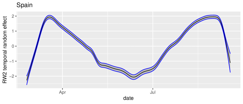
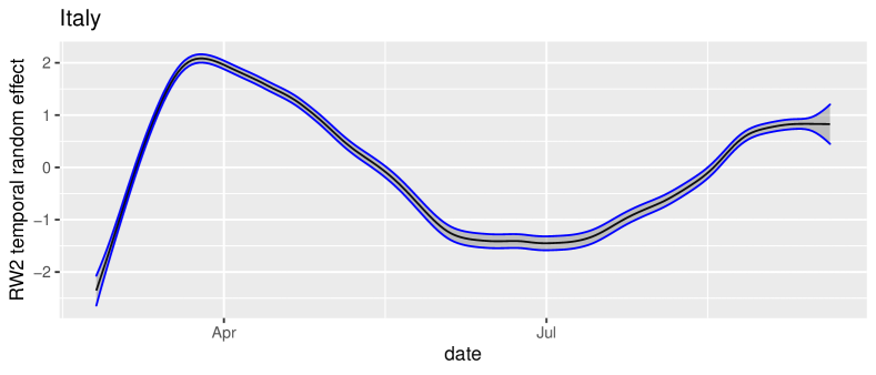
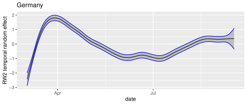
The Bayesian estimates and 95% credible intervals for the temporal trend $\delta_{t}$, $t=1,\ldots,T$, are shown in Figure 1. These plots can be interpreted as a smoothed temporal trend of the relative risk in the whole country. In fact, Figure 1 suggests that the COVID-19 epidemic in all three countries rapidly reached their peaks and slowly started to decline at the beginning of April and then increased and reached its maximum in August. In addition, the second wave of the epidemic seems to be stronger in Spain and Germany shows a more smoother trend during the study period.

Figure 2: Posterior mean of the spatial random effects $\zeta_{i}$ (left) and $\xi_{i}$ (right) in the fitted model

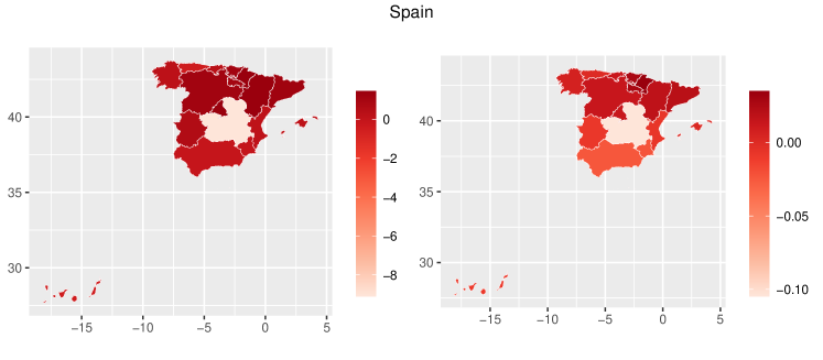
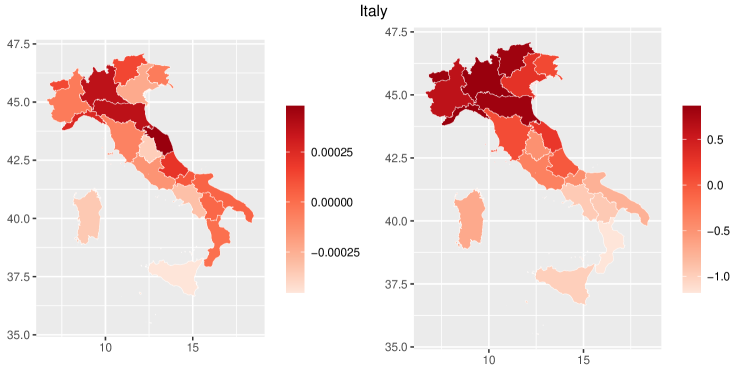
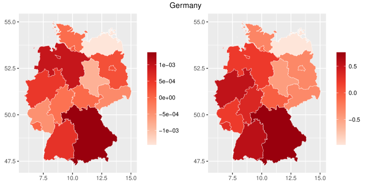
Figure 2 shows the the posterior means of the spatial random effects $\zeta_{i}$ and $\xi_{i}$, $i=1,\ldots,m$, on the corresponding map of each country. The plot illustrates spatial heterogeneity of the relative risk of COVID-19 across regions in each country, particularly in Spain. Regions with positive (negative) $\zeta_{i}+\xi_{i}$ values are expected to have elevated (lower) relative risks than the the baseline country-wide risk during the study period.

Figure 3: Observed value (solid line), predicted value (dashed line) and 95% prediction interval (grey area) for the daily number of new COVID-19 cases in the whole country, based on the posterior mean and 95% credible interval of the spatially accumulated relative risks of the fitted model

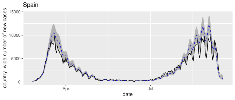
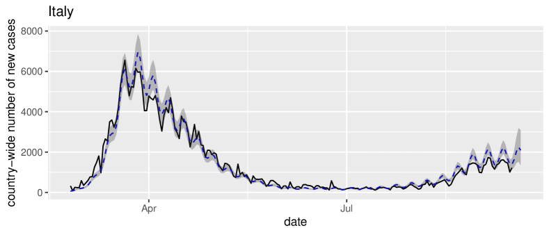
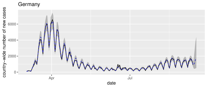
In order to see how the estimated relative risks under the fitted model are in agreement with the observed data, Figure 3 shows the spatially accumulated daily number of cases $\sum_{i=1}^{m}Y_{it}$, $t=1,\ldots,T$, and their expected values under the fitted model, namely the posterior mean and 95% credible interval of $\sum_{i=1}^{m}\widehat{E}_{it}\widehat{\theta}_{it}$, $t=1,\ldots,T$. Except some discrepancies for Spain and Italy, the observed values are inside the 95% credible intervals and close to the expected values under the fitted model. Figure 3 in addition shows 4-days ahead forecasts of the total daily number of new cases at the end of study period of each country.

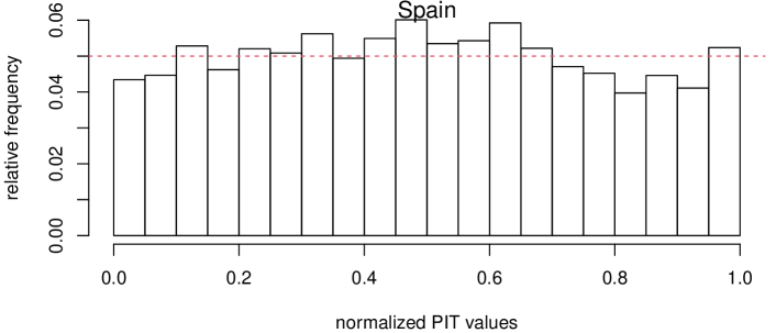
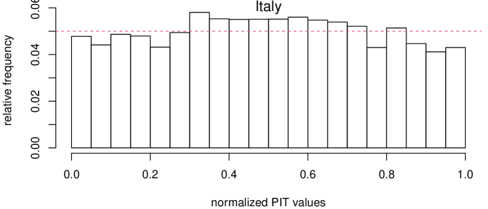
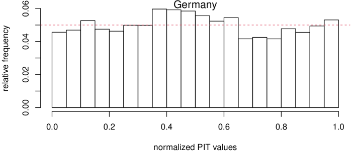
Finally, histograms of the normalized PIT values described in Section 4.4 are obtained using $J=20$ from the fitted models and plotted in Figure 4. The normalized PIT values for the fitted models to data do not show a clear visible pattern and the histograms seems to be close to the standard uniform distribution.

Figure 4: Histograms of normalized PIT values to check for uniformity

The above results and more details on observed and predicated values from the fitted model are also provided in an interactive Shiny web application at https://ajalilian.shinyapps.io/shinyapp/.

6 Concluding remarks

There are some limitations in the analyses and modeling of data on the number of new cases of COVID-19, including data incompleteness and inaccuracy, unavailability or inaccuracy of relevant variables such as population movement and interaction, as well as the unknown nature of the new COVID-19 virus. Nevertheless, understanding the underlying spatial and temporal dynamics of the spread of COVID-19 can result in detecting regional or global trends and to further make informed and timely public health policies such as resource allocation.

In this study, we used a spatio-temporal model to explain the spatial and temporal variations of the relative risk of the disease in Spain, Italy and Germany. Despite data limitations and the complexity and uncertainty in the spread of COVID-19, the model was able to grasp the temporal and spatial trends in the data. However, the posterior predictive checks using the normalized probability integral transform (PIT) showed that there is room for the model improvements.

Obliviously, there are many relevant information and covariates that can be considered in our modeling framework and improve the model’s predictive capabilities. One good possibility would be considering most recent and accurate human mobility amongst regions. We would expect our model would benefit from this information, which right now can not be accessed. Moreover, the considered spatio-temporal model in this paper is one instance among many possibilities. For example, one possibility is to include a random effect term in the model that represents variations due to joint spatio-temporal correlations; e.g., a separable sptaio-temporal covariance structure. However, the considered model was adequate and no joint spatio-temporal random effect term was considered to avoid increasing the model’s complexity.

We focused here on a stochastic spatio-temporal model as a good alternative to existing deterministic compartmental models in epidemiology to explain the spatio-temporal dynamics in the spread of COVID-19. However, it should be emphasized that one step forward would be considering a combination of a deterministic compartmental model in terms of differential equations for the number of susceptible, exposed, infectious and recovered cases with our sort of stochastic modeling approach. This is a clear novelty and a direction for future research.

Conflict of interest

The authors declare that they have no conflict of interest.

References

- Alamo et al., (2020) Alamo, T., Reina, D. G., Mammarella, M., and Abella, A. (2020). Open data resources for fighting covid-19. arXiv preprint arXiv:2004.06111.
- Anderson and Ryan, (2017) Anderson, C. and Ryan, L. M. (2017). A comparison of spatio-temporal disease mapping approaches including an application to ischaemic heart disease in new south wales, australia. International journal of environmental research and public health, 14(2):146.
- Bastos and Cajueiro, (2020) Bastos, S. B. and Cajueiro, D. O. (2020). Modeling and forecasting the covid-19 pandemic in brazil. arXiv preprint arXiv:2003.14288.
- Besag et al., (1991) Besag, J., York, J., and Mollié, A. (1991). Bayesian image restoration, with two applications in spatial statistics. Annals of the institute of statistical mathematics, 43(1):1–20.
- Briz-Redón and Serrano-Aroca, (2020) Briz-Redón, Á. and Serrano-Aroca, Á. (2020). A spatio-temporal analysis for exploring the effect of temperature on covid-19 early evolution in spain. Science of The Total Environment, page 138811.
- Center International Earth Science Information Network Columbia University, 2018 (CIESIN) Center International Earth Science Information Network (CIESIN) Columbia University (2018). Gridded population of the world, version 4 (gpwv4): Population count, revision 11. https://doi.org/10.7927/H4JW8BX5. Accessed 15 May 2020.
- Chang et al., (2020) Chang, W., Cheng, J., Allaire, J., Xie, Y., and McPherson, J. (2020). shiny: Web Application Framework for R. R package version 1.4.0.2.
- Consul and Jain, (1973) Consul, P. C. and Jain, G. C. (1973). A generalization of the poisson distribution. Technometrics, 15(4):791–799.
- Czado et al., (2009) Czado, C., Gneiting, T., and Held, L. (2009). Predictive model assessment for count data. Biometrics, 65(4):1254–1261.
- Danon et al., (2020) Danon, L., Brooks-Pollock, E., Bailey, M., and Keeling, M. J. (2020). A spatial model of covid-19 transmission in england and wales: early spread and peak timing. medRxiv.
- Dawid, (1984) Dawid, A. P. (1984). Present position and potential developments: Some personal views statistical theory the prequential approach. Journal of the Royal Statistical Society: Series A (General), 147(2):278–290.
- Fahrmeir and Kneib, (2008) Fahrmeir, L. and Kneib, T. (2008). On the identification of trend and correlation in temporal and spatial regression. In Recent advances in linear models and related areas, pages 1–27. Springer.
- Gayawan et al., (2020) Gayawan, E., Awe, O., Oseni, B. M., Uzochukwu, I. C., Adekunle, A. I., Samuel, G., Eisen, D., and Adegboye, O. (2020). The spatio-temporal epidemic dynamics of covid-19 outbreak in africa. medRxiv.
- Giuliani et al., (2020) Giuliani, D., Dickson, M. M., Espa, G., and Santi, F. (2020). Modelling and predicting the spatio-temporal spread of coronavirus disease 2019 (covid-19) in italy. Available at SSRN 3559569.
- Gross et al., (2020) Gross, B., Zheng, Z., Liu, S., Chen, X., Sela, A., Li, J., Li, D., and Havlin, S. (2020). Spatio-temporal propagation of covid-19 pandemics.
- Kandel et al., (2020) Kandel, N., Chungong, S., Omaar, A., and Xing, J. (2020). Health security capacities in the context of covid-19 outbreak: an analysis of international health regulations annual report data from 182 countries. The Lancet.
- Kang et al., (2020) Kang, D., Choi, H., Kim, J.-H., and Choi, J. (2020). Spatial epidemic dynamics of the covid-19 outbreak in china. International Journal of Infectious Diseases.
- Langousis and Carsteanu, (2020) Langousis, A. and Carsteanu, A. A. (2020). Undersampling in action and at scale: application to the COVID-19 pandemic. Stochastic Environmental Research and Risk Assessment, 34(8):1281–1283.
- Lawson, (2018) Lawson, A. B. (2018). Bayesian Disease Mapping: Hierarchical Modeling in Spatial Epidemiology. Chapman and Hall/CRC, 3 edition.
- Lee, (2011) Lee, D. (2011). A comparison of conditional autoregressive models used in bayesian disease mapping. Spatial and spatio-temporal epidemiology, 2(2):79–89.
- Lindgren et al., (2015) Lindgren, F., Rue, H., et al. (2015). Bayesian spatial modelling with r-inla. Journal of Statistical Software, 63(19):1–25.
- Martins et al., (2013) Martins, T. G., Simpson, D., Lindgren, F., and Rue, H. (2013). Bayesian computing with inla: new features. Computational Statistics & Data Analysis, 67:68–83.
- Peng et al., (2020) Peng, L., Yang, W., Zhang, D., Zhuge, C., and Hong, L. (2020). Epidemic analysis of covid-19 in china by dynamical modeling. arXiv preprint arXiv:2002.06563.
- Pettit, (1990) Pettit, L. (1990). The conditional predictive ordinate for the normal distribution. Journal of the Royal Statistical Society: Series B (Methodological), 52(1):175–184.
- Riebler et al., (2016) Riebler, A., Sørbye, S. H., Simpson, D., and Rue, H. (2016). An intuitive bayesian spatial model for disease mapping that accounts for scaling. Statistical methods in medical research, 25(4):1145–1165.
- Roda et al., (2020) Roda, W. C., Varughese, M. B., Han, D., and Li, M. Y. (2020). Why is it difficult to accurately predict the covid-19 epidemic? Infectious Disease Modelling.
- Rue et al., (2009) Rue, H., Martino, S., and Chopin, N. (2009). Approximate bayesian inference for latent gaussian models by using integrated nested laplace approximations. Journal of the royal statistical society: Series b (statistical methodology), 71(2):319–392.
- Sujath et al., (2020) Sujath, R., Chatterjee, J. M., and Hassanien, A. E. (2020). A machine learning forecasting model for COVID-19 pandemic in india. Stochastic Environmental Research and Risk Assessment, 34(7):959–972.
- Wakefield, (2007) Wakefield, J. (2007). Disease mapping and spatial regression with count data. Biostatistics, 8(2):158–183.
- Waller et al., (1997) Waller, L. A., Carlin, B. P., Xia, H., and Gelfand, A. E. (1997). Hierarchical spatio-temporal mapping of disease rates. Journal of the American Statistical association, 92(438):607–617.
- World Health Organization, (2020) World Health Organization (2020). Coronavirus disease (covid-19) outbreak. URL https://www.who.int/emergencies/diseases/novel-coronavirus-2019.
- Zamani and Ismail, (2012) Zamani, H. and Ismail, N. (2012). Functional form for the generalized poisson regression model. Communications in Statistics-Theory and Methods, 41(20):3666–3675.