Experimental Parameter Analysis
of the Reservoirs Observers
using Echo State Network Approach

Abstract

Dynamical systems has a variety of applications for the new information generated during the time. Many phenomenons like physical, chemical or social are not static, then an analysis over the time is necessary. In this work, an experimental analysis of parameters of the model Echo State Network is performed and the influence of the kind of Complex Network is explored to understand the influence on the performance. The experiments are performed using the Rossler attractor.

I INTRODUCTION

Frequently, chaos is associated with disorder, instability, inconsistency, no control and so on, a common phenomenon in the nature. Using a formal definition, chaos is the irregular movement observed in non linear deterministic dynamical systems From the chaos perspective, many temporal series are understood and analyzed. There is a increasing interest to predict temporal series because they can represent real phenomenons. By consequence, many methods based on kernel as Support Vector Machine[1], Relevant Vector Machine (RVM)[2] and neural network models: Multilayer perceptron[3], Radial Basis Function Neural Network[4], Recurrent Predictor Neural Network[5], Elman Network[6], and Echo state network (ESN)[7]. Besides, other methods based on Fuzzy Model[8], Extended Kalman filter[9].

Recurrent Neural Networks are a powerful tool based on biological brain, there is a great diversity of applications. However, the main difficulty is the training step, because all the weights of the network must be trained[10].

Reservoir computing (RC) is a recent technique of Machine Learning based on the design of Recurrent Networks, the difference is the simplicity of the training step, only a the weights of output layer is trained. Echo State Network Models(ESNs), Liquid State Machines(LSMs), Backpropagation Decorrelation Neural Networks and Evolution of Systems with Linear Outputs(Evolino) are examples of RC. [11], proposed ESN to find a way of predicting temporal series.

ESN is a kind of RNNS with a features of simplicity and less computational cost. ESN classical models are build using a big number of neurons with sparse and random connections where only weights of output layer are trained. ESN has big potential for non linear approximation problems and his use is big in the prediction of temporal series: Identification Systems[12], Modeling neural plasticity for classification and regression[13], Time series Prediction [7], Pattern Recognition[14].

The reservoir of a ESN is used as processing layer and this is not modified during training phase. For a good performance of ESN, the reservoir must satisfied a condition about his state dynamics(echo property), the state of reservoir is an echo of the history of his inputs. Spectral Radius of the reservoir has a high impact over the performance model and his capacity of good estimations[10].

Complex Networks are added to the design of the reservoir dynamics of original model of ESN to imitate the way how learning mechanisms of real world works, like Small World and Free Scale Complex Networks[15]. Giving ESN the potential of solving non linear modelling problems and prediction of chaotic temporal series, showing similar features of biological neural networks, like a power-law distribution, small-word feature, community structure, and distributed architecture[16].

Small World is a feature in a Complex Network with high degree of clustering with a property of a high number of connections between closest nodes forming a small world. In contrast, Free Scale, the connection of nodes is represented by Potency Law. Recently, Neural Networks with Complex Network Topology presented better performance than classical ones[17, 18].

The present work is organized: in Section II, a literature review of ESN and extentions are presented. In Section III, a briefly description ESN is summarized, in Section IV the results of experiments are presented. Finally, Section V states with the conclusions.

II LITERATURE REVIEW

The classic ESN model has recently been criticized[19] for the fact that the reservoir is generated randomly, as well as the connections of the internal units. This fact causes high complexity in the performance on the model and in many cases does not guarantee the stability of the prediction. This is because the classic ESN model has difficulties due to the lack of information about the understanding and the properties of the reservoir, such as connection configuration and weight allocation, it does not guarantee an optimal configuration. In addition to, it does not providing a clear view of the design and structure about model. That’s the reason which motivated many researchers to carry out studies in order to find those parameters that optimize and guarantee the stability of the solution.

As a solution to the randomness’ problem, several studies have been developed, finding two strong approaches: modification of weights [20] and modification of the reservoir’s structure[16]. On the other hand, Multiple Loops Reservoir structure (MLR) model[21] was proposed and compared to the Adjacent-feedback loop Resevoir (ALR) model, MLR strengthens the connections within the reservoir and improves the skills of the classic model for the nonlinear approach. The work also analyzes the influence of the parameters of the proposed model based in the prediction accuracy. Attending to the same goal, in 2014, a new ESN model known as Simple Cycle Reservoir Network (SCRN)[22] was introduced, where the reservoir was constructed deterministically. Initially the proposal considered a reservoir of size larger than required and using a pruning algorithm, in this case, the Sensitive Iterated Pruning Algorithm algorithm (SIPA) then the less sensitive neurons are turned off to optimize the number of required neurons to reach a good approximation. In the work [15], a design of clustered complex echo state network is formulated for the forecast of mobile communications traffic using the Fourier spectrum as prior knowledge to generate the functional clusters.

The performance of an ESN network is closely related to its learning paradigm, that is, the training algorithms used, which can be categorized in two ways: batch learning and online sequential learning. In batch learning, the constant system weights are fixed while calculating the error associated with each sample in the input. Whereas the online sequential learning weights are constantly updated, and error (and, therefore, the gradient estimate), so that different weights are used for each input sample. In the online sequential learning scheme the data is processed sequentially as well as the network topology is adapted. RNNs have been widely used following this type of approach.

Recently, in [23], the OSESN-RLS (Online Sequential ESN with Sparse Recursive Least Squares) algorithm was proposed, which controls the size of the network using the penalty restrictions of the $l_{0}$ and $l_{1}$ norms into the error criterion.

In addition to the learning paradigm, the effectiveness of this type of networks is strongly influenced by the size of the reservoir. According to [10], the fact that the network is generated randomly means that a greater amount of neurons is needed, because a memory capacity in an network with dynamic reservoir with $N$ nodes is always lower than of amount of reservoir’s units in comparison to traditional neural networks, being one of the possible causes of overfitting. As an alternative solution to this problem, evolutionary algorithms have been used [24, 25] to find an optimal number of neurons for the reservoir, the disadvantage is the computational cost, experience and skill abilities of those who use them. Recently, in [26] Leaky-ESN was proposed, modifying the reservoir units of a classic ESN to replace them with leaky integrator units, facilitating learning of slow dynamics[27]. This method considers the output feedback line in the network, thus maintaining the natural essence of a recurring network that generally ignores this type of connections. In addition to, it modifies the sufficient conditions for the echo condition and uses the barrier method to optimize the control of the network parameters.

III ESN MODEL

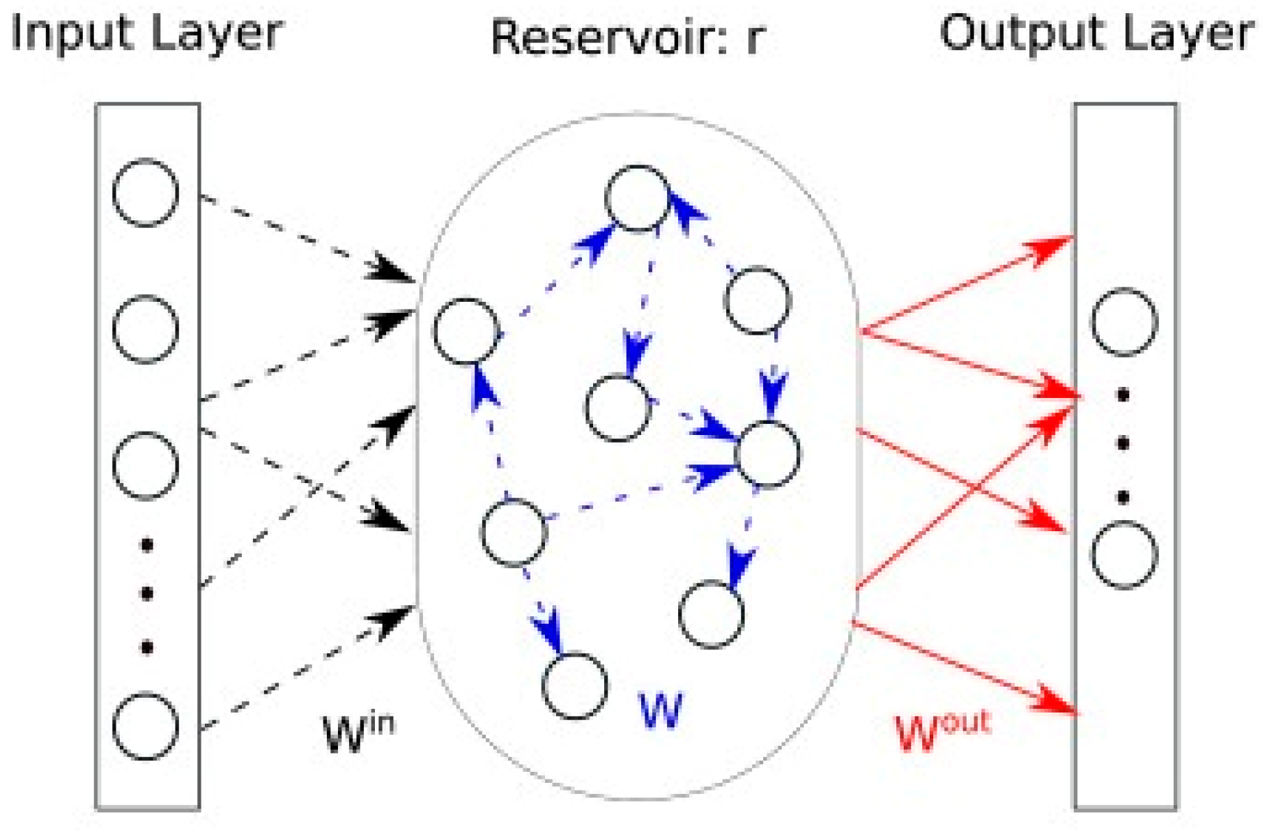
The Echo state network (ESN) neural network model is a new and robust type of recurring network that has a special configuration. It consists of a network whose hidden layer is a reservoir with a certain number of neurons, where only the weights of the network are trained during the learning phase. For this model to work, it is necessary that the dynamics of the reservoir be less chaotic as possible, it is known as “ echo property”. According to Jaeger (2002)[10], we define the previously assumption in the next definition.

Definition 1 (Echo property).

A network has the echo status property if the current state of the network is only determined by the values of the past inputs and outputs. In other words for each internal unit of the $r_{i}$ reservoir, there is a $e_{i}$ function, which is known as an echo function, which maps the input/output pair ($x_{i},y_{i}$) of its history to the current state. Thus the current state for one reservoir’s unit $r_{i}(n)$ in the time instance $t$ is given by the equation (1)

$$r_{i}(n)=e_{i}((x(n),y(n)),(x(n-1),y(n-1)),\dots)$$ (1)

We are going to consider in the case of time a RNN that has $K$ input units $\mathbf{x}=(x_{1},x_{2},x_{3},\dots,x_{K})$, a hidden layer consisting of a reservoir with N internal units, $\mathbf{r}=(r_{1},r_{2},r_{3},\dots,r_{N})$, where $\mathbf{r}$ represents the system state vector for some time of time $t$, and a output layer with $L$ units, $\mathbf{y}=(y_{1},y_{2},y_{3},\dots,y_{L})$. The weights of the connections between the neurons are stored in the adjacency matrices $W_{in},W,W_{out},W_{back}$ (the last case matrix only if exists feedback), where $W$ is a matrix which stored the weights of the resevoir’s units. The sizes of these matrices are $N\times K,N\times N,L\times(K+N+L),N\times L$, respectively. The figure 1 shows an example of the architecture of a ESN classical model.

Figure 1: Basic setup of ESN[28].

For the implementation of the model we follow the design and ideas proposed in [29]. Therefore, the activation function for the internal units of the reservoir is given by the equation

$$\mathbf{r}(n+1)=(1-\alpha)\mathbf{r}(t)+\alpha f(W\mathbf{r}(t)+W_{in}\mathbf{x}(t)+\zeta)$$

where $0<\alpha\leq 1$ is “ the leakage rate” which causes the reservoir to evolve more slowly as $\alpha\longrightarrow 0$, $\zeta$ bias and the function $f=tanh$. On the other hand, the output of the network is given by the equation

$$\mathbf{y}(t)=W_{out}\mathbf{r}(t)+c$$

The adjacency matrix of the reservoir, $W$, is obtained through the different configurations of the complex network designs used in the experiments. According to Jaeger(2001)[10], the echo property for a neural network is closely related to the algebraic properties of the reservoir adjacency matrix, so that a condition necessary for the echo property to be guaranteed is that said matrix has a spectral radius of less than 1. So in this case, we scale the $W$ matrix so that we guarantee that the model works.

IV EXPERIMENTS AND RESULTS

IV-A Problem

Let be a dynamical system: $d\phi/dt=f(\phi)$ and input, output vector of the system: $\mathbf{x}(t),\mathbf{y}(t)$. Where $\phi$ represents the state of the system. In this problem, $\mathbf{x}\in\mathbb{R}^{N}$ and $\mathbf{y}\in\mathbb{R}^{M}$ are known during the interval of time $[0,T]$ para $T\in\mathbb{R}$.

IV-B Purpose

The main objective is to estimate the values of $\mathbf{y}$ for a time $t>T$, from knowing the value of $\mathbf{x}$, this is known as an ‘observer”[29]. For this task, a technique from Machine Learning is used, “reservoir computing”. This network originally proposed by Jaeger y Haas[11]. A experimental analysis of the parameters were performed and make an adaptation to change the complex network architecture to analyze the influence of the kind of CN to know the performance, benefits and restrictions.

Rossler Atractor Dynamical System

Let consider the next equation system:

$$\begin{cases}dx/dt=-y-z,\\ dy/dt=x+ay,\\ dz/dt=b+z(x-c)\end{cases}$$ (2)

then the study is on the Equation Eq. 2 for the instance of $a=0.5$, $b=2.0$ y $c=4.0$. For the experiment, the known and available variable is $x$ so $x$ is the input with the information of the variables $y$ y $z$ together in the interval of time $[T_{0},T_{1}]$, for $T_{0}>0$. The data used in this experiment was obtained by solving the equation’s system described in (2) using Runge Kutta 4th order method, with $0.1$ time step.

number of reservoir nodes: $$N=400$$

spectral radius: $$\rho=1$$

average degree: $$D=20$$

bias constant: $$\zeta=1$$

leakage rate: $$\alpha=1$$

time step: $$\textrm{delta }t=0.1$$

initial time: $$T_{0}=100$$

initial time of training phase: $$T_{1}=260$$

final time of predicted phase: $$T_{2}=500$$

The values of the tested parameters follows the next criterion: $List\_X$ = A:inc:B, the list starts with $A$ value to $B$ and an increment of $inc$.

IV-C Number of Reservoir Nodes

The values of N tested: $List_{N}$ = 50:50:2000. The Figure Fig. 2 presents the results of varying the number of reservoir nodes.

Figure 2: ESN model performance using Erdos Renyi, varying the number of neurons into the reservoir

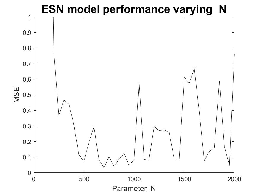
The best results are around the interval [$600$, $900$] neurons.

IV-D Mean Degree of The Connections

The values of parameter $D$: $List\_D$=10:20:390. The graphic Fig.3 presents the results of different mean degree.

Figure 3: ESN model performance using Erdos Renyi, varying the mean degree into the reservoir

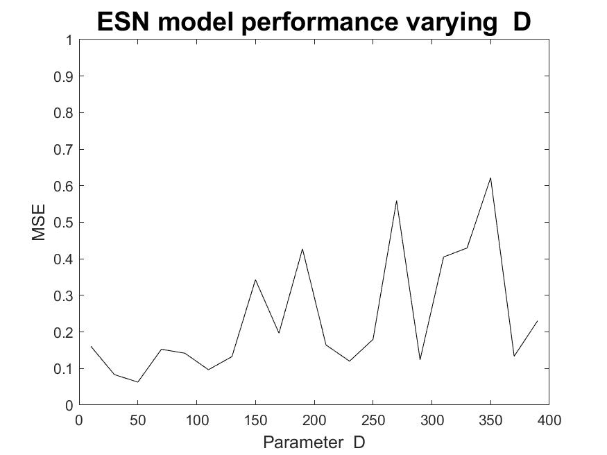
In contrast of the previous parameter N, this parameter presents more specific good values, around $50$.

IV-E Initial Time for Training Step

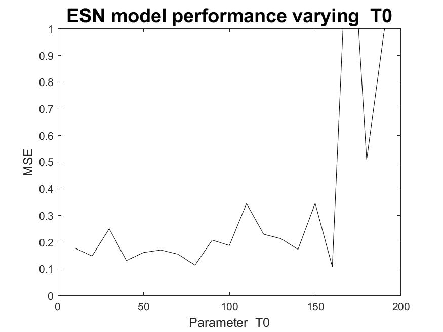
Values for parameter $T0$, $List\_T0$ = 10:10:200. The plot presented in Fig. 4 present the MSE values for parameter $T0$.

Figure 4: ESN model performance using Erdos Renyi, varying the initial time instance of training phase

IV-F Initial/Final time for Prediction Step

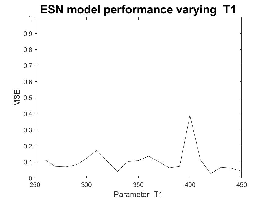
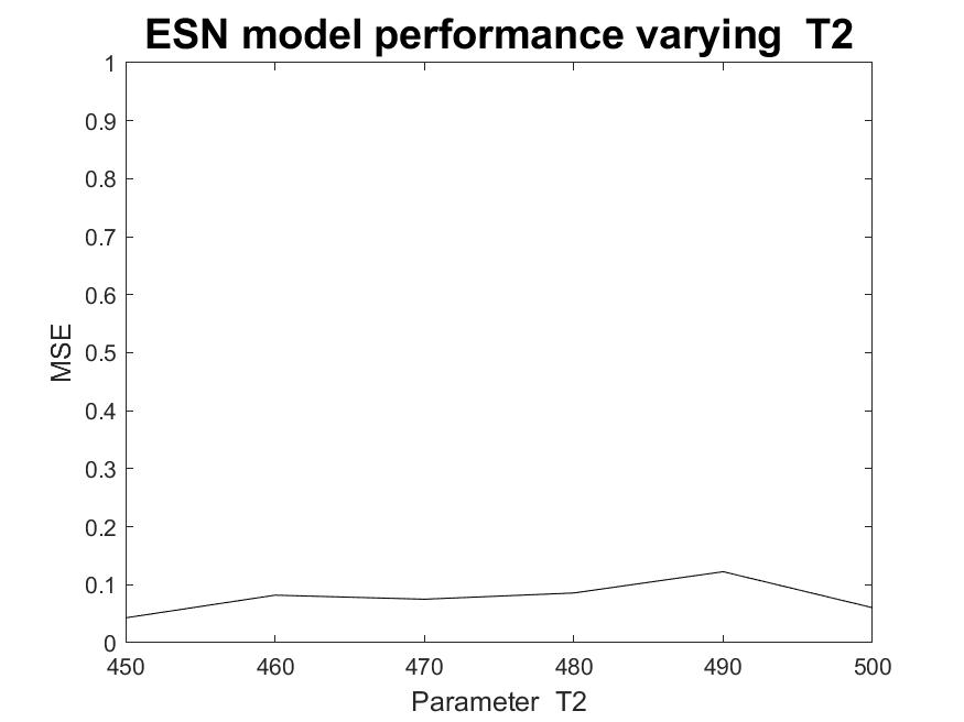
The values for parameters $T1$ and $T2$ are: $List\_T1$ = 260:10:450 and $List\_T2$ = 450:10:800, respectively. The figure Fig. 5 and 6 presents the results for the experiment.

Figure 5: ESN model performance using Erdos Renyi, varying the initial time instance of prediction phase

Figure 6: ESN model performance using Erdos Renyi, varying the final time instance for prediction phase

IV-G Time Step for Prediction phase

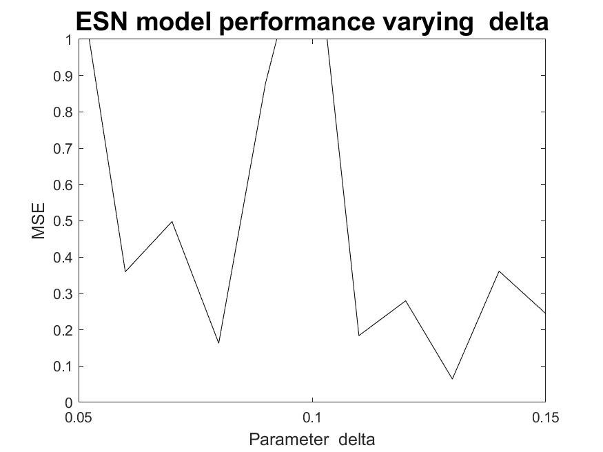
The graphic Fig. 7 shows the values for parameter $delta$.

Figure 7: ESN model performance using Erdos Renyi, varying the parameter delta

From the figures: Fig. 2, 3, 4, 5,6, 7. The first analyzis shows that the parameter $N$ and $D$, $delta$ presents higher inestability or influence with a variation of their values. In contrast, parameter $T0$, $T1$ and $T2$ has high stability or less variance in MSE values.

IV-H Complex Network Architecture

In the table Tab. I, a variation of MSE(minimal square error) is presented with the change of Complex Network Architecture for the ESN model[29]. The Complex Networks tested were: Erd$\ddot{o}$s Renyi, Barabási, Small world and Random Matrix(reservoir randomly generated)

TABLE I: MSE of ESN model varying the reservoir’s configuration

Reservoir	MSE
Erd$\ddot{o}$s Renyi	0.0669
Random Matrix	0.1811
Barabási	0.0808
Small World	0.1638

From the table Tab. I, the best was Erd$\ddot{o}$s Renyi. However, the differences between the architectures are not high.

The next graphics Fig. 8 are the result of considering the same criterion of previous experiments using different complex network architecture to analyze visually the impact of the parameters over the performance.

Figure 8: Results of Parameter Variation for Different Complex Network Architecture

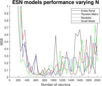
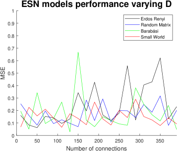
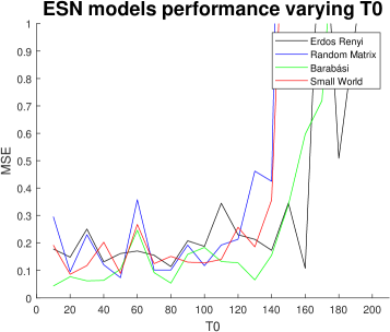
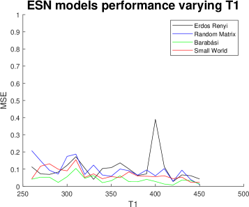
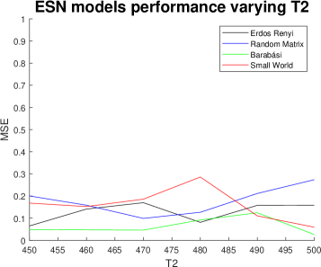
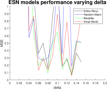
From the results presented in the figure Fig. 8, a similar conclusion than previous experiments only using original EsN can be stated. Parameters $N$, $D$ and $delta$ has higher variance in MSE values but a new parameter is found $T0$, the other parameters has less variance. Besides, there is a different behaviour using many kind of Complex Networks and the architecture with similar performance than Erdos Renyi(original ESN model) is Small World even this model overperform Erdos Renyi.

V CONCLUSION

Following the results of the experiments of this work, we can conclude that some parameters studied are potentially influencers than others in the performance for each original ESN model and the performance is very sensible to variety of them. In some cases, a reservoir with a certain configuration(Complex Network architecture) can adjusted with precision to the training data, but at the same time, this fact can generate a deficient generalization and high computational cost, due the reservoirs are constructed based in randomness.

References

- [1] T. Van Gestel, J. A. K. Suykens, D. . Baestaens, A. Lambrechts, G. Lanckriet, B. Vandaele, B. De Moor, and J. Vandewalle, “Financial time series prediction using least squares support vector machines within the evidence framework,” IEEE Transactions on Neural Networks, vol. 12, no. 4, pp. 809–821, July 2001.
- [2] A. F. Khalil, M. McKee, M. Kemblowski, T. Asefa, and L. Bastidas, “Multiobjective analysis of chaotic dynamic systems with sparse learning machines,” Advances in Water Resources, vol. 29, no. 1, pp. 72 – 88, 2006.
- [3] N. Stamatis, D. Parthimos, and T. M. Griffith, “Forecasting chaotic cardiovascular time series with an adaptive slope multilayer perceptron neural network,” IEEE Transactions on Biomedical Engineering, vol. 46, no. 12, pp. 1441–1453, Dec 1999.
- [4] Henry Leung, Titus Lo, and Sichun Wang, “Prediction of noisy chaotic time series using an optimal radial basis function neural network,” IEEE Transactions on Neural Networks, vol. 12, no. 5, pp. 1163–1172, Sep. 2001.
- [5] Min Han, Jianhui Xi, Shiguo Xu, and Fu-Liang Yin, “Prediction of chaotic time series based on the recurrent predictor neural network,” IEEE Transactions on Signal Processing, vol. 52, no. 12, pp. 3409–3416, Dec 2004.
- [6] M. Ardalani-Farsa and S. Zolfaghari, “Chaotic time series prediction with residual analysis method using hybrid elman–narx neural networks,” Neurocomputing, vol. 73, no. 13, pp. 2540 – 2553, 2010, pattern Recognition in Bioinformatics Advances in Neural Control.
- [7] D. Li, M. Han, and J. Wang, “Chaotic time series prediction based on a novel robust echo state network,” IEEE Transactions on Neural Networks and Learning Systems, vol. 23, no. 5, pp. 787–799, May 2012.
- [8] Y. J. Mao Jian-Qin, Ding Hai-Shan, “Chaotic time series prediction based on fuzzy tree,” Acta Physica Sinica, vol. 58, no. 4, p. 2220, 2009.
- [9] X. Hu, D. V. Prokhorov, and D. C. W. II, “Time series prediction with a weighted bidirectional multi-stream extended kalman filter,” Neurocomputing, vol. 70, no. 13, pp. 2392 – 2399, 2007, selected papers from the 3rd International Conference on Development and Learning (ICDL 2004) Time series prediction competition: the CATS benchmark.
- [10] H. Jaeger, “A tutorial on training recurrent neural networks, covering bppt, rtrl, ekf and the ”echo state network” approach,” 2005.
- [11] ——, “The”echo state”approach to analysing and training recurrent neural networks,” 2001.
- [12] ——, “Adaptive nonlinear system identification with echo state networks,” in NIPS, 2002.
- [13] M.-H. Yusoff, J. Chrol-Cannon, and Y. Jin, “Modeling neural plasticity in echo state networks for classification and regression,” Information Sciences, vol. 364-365, pp. 184 – 196, 2016. [Online]. Available: http://www.sciencedirect.com/science/article/pii/S0020025515008270
- [14] M. D. Skowronski and J. G. Harris, “Noise-robust automatic speech recognition using a discriminative echo state network,” in 2007 IEEE International Symposium on Circuits and Systems, May 2007, pp. 1771–1774.
- [15] P. Yu, L. Miao, and G. Jia, “Clustered complex echo state networks for traffic forecasting with prior knowledge,” in 2011 IEEE International Instrumentation and Measurement Technology Conference, May 2011, pp. 1–5.
- [16] E. Najibi and H. Rostami, “Scesn, spesn, swesn: Three recurrent neural echo state networks with clustered reservoirs for prediction of nonlinear and chaotic time series,” Applied Intelligence, vol. 43, no. 2, pp. 460–472, Sep 2015.
- [17] J. W. Bohland and A. A. Minai, “Efficient associative memory using small-world architecture,” Neurocomputing, vol. 38-40, pp. 489 – 496, 2001, computational Neuroscience: Trends in Research 2001.
- [18] D. Stauffer, A. Aharony, L. da Fontoura Costa, and J. Adler, “Efficient hopfield pattern recognition on a scale-free neural network,” The European Physical Journal B - Condensed Matter and Complex Systems, vol. 32, no. 3, pp. 395–399, Apr 2003.
- [19] H. Jaeger, W. Maass, and J. Principe, “Editorial: Special issue on echo state networks and liquid state machines,” Neural Netw., vol. 20, no. 3, pp. 287–289, Apr. 2007.
- [20] H. Wang and X. Yan, “Optimizing the echo state network with a binary particle swarm optimization algorithm,” Knowledge-Based Systems, vol. 86, pp. 182 – 193, 2015.
- [21] L. Sun, X. Yang, J. L. Zhou, J. Wang, and F. Xiao, “Echo state network with multiple loops reservoir and its application in network traffic prediction,” 2018 IEEE 22nd International Conference on Computer Supported Cooperative Work in Design ((CSCWD)), pp. 689–694, 2018.
- [22] H. Wang and X. Yan, “Improved simple deterministically constructed cycle reservoir network with sensitive iterative pruning algorithm,” Neurocomputing, vol. 145, pp. 353 – 362, 2014.
- [23] C. Yang, J. Qiao, Z. Ahmad, K. Nie, and L. Wang, “Online sequential echo state network with sparse rls algorithm for time series prediction,” Neural Networks, vol. 118, pp. 32 – 42, 2019.
- [24] S. Otte, M. V. Butz, D. Koryakin, F. Becker, M. Liwicki, and A. Zell, “Optimizing recurrent reservoirs with neuro-evolution,” Neurocomputing, vol. 192, pp. 128 – 138, 2016, advances in artificial neural networks, machine learning and computational intelligence. [Online]. Available: http://www.sciencedirect.com/science/article/pii/S0925231216002629
- [25] H. Wang and X. Yan, “Optimizing the echo state network with a binary particle swarm optimization algorithm,” Knowledge-Based Systems, vol. 86, pp. 182 – 193, 2015. [Online]. Available: http://www.sciencedirect.com/science/article/pii/S095070511500221X
- [26] S. xian Lun, H. feng Hu, and X. shuang Yao, “The modified sufficient conditions for echo state property and parameter optimization of leaky integrator echo state network,” Applied Soft Computing, vol. 77, pp. 750 – 760, 2019.
- [27] G. Boffetta, A. Crisanti, F. Paparella, A. Provenzale, and A. Vulpiani, “Slow and fast dynamics in coupled systems: A time series analysis view,” Physica D: Nonlinear Phenomena, vol. 116, no. 3, pp. 301 – 312, 1998. [Online]. Available: http://www.sciencedirect.com/science/article/pii/S016727899700300X
- [28] Q.-u.-a. Mastoi, T. Y. Wah, and R. Gopal Raj, “Reservoir computing based echo state networks for ventricular heart beat classification,” Applied Sciences, vol. 9, no. 4, 2019. [Online]. Available: https://www.mdpi.com/2076-3417/9/4/702
- [29] Z. Lu, J. Pathak, B. Hunt, M. Girvan, R. Brockett, and E. Ott, “Reservoir observers: Model-free inference of unmeasured variables in chaotic systems,” Chaos: An Interdisciplinary Journal of Nonlinear Science, vol. 27, no. 4, p. 041102, 2017. [Online]. Available: https://doi.org/10.1063/1.4979665