‘Less Than One’-Shot Learning:
Learning N Classes From M<N Samples
Abstract
Deep neural networks require large training sets but suffer from high computational cost and long training times. Training on much smaller training sets while maintaining nearly the same accuracy would be very beneficial. In the few-shot learning setting, a model must learn a new class given only a small number of samples from that class. One-shot learning is an extreme form of few-shot learning where the model must learn a new class from a single example. We propose the ‘less than one’-shot learning task where models must learn new classes given only examples and we show that this is achievable with the help of soft labels. We use a soft-label generalization of the k-Nearest Neighbors classifier to explore the intricate decision landscapes that can be created in the ‘less than one’-shot learning setting. We analyze these decision landscapes to derive theoretical lower bounds for separating classes using soft-label samples and investigate the robustness of the resulting systems.
Introduction
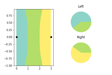
Deep supervised learning models are extremely data-hungry, generally requiring a very large number of samples to train on. Meanwhile, it appears that humans can quickly generalize from a tiny number of examples (Lake, Salakhutdinov, and Tenenbaum 2015). Getting machines to learn from ‘small’ data is an important aspect of trying to bridge this gap in abilities. Few-shot learning (FSL) is one approach to making models more sample efficient. In this setting, models must learn to discern new classes given only a few examples per class (Lake, Salakhutdinov, and Tenenbaum 2015; Snell, Swersky, and Zemel 2017; Wang et al. 2020). Further progress in this area has enabled a more extreme form of FSL called one-shot learning (OSL); a difficult task where models must learn to discern a new class given only a single example of it (Fei-Fei, Fergus, and Perona 2006; Vinyals et al. 2016). In this paper, we propose ‘less than one’-shot learning (LO-shot learning), a setting where a model must learn new classes given only examples, less than one example per class. At first glance, this appears to be an impossible task, but we both theoretically and empirically demonstrate feasibility. As an analogy, consider an alien zoologist who arrived on Earth and is being tasked with catching a unicorn. It has no familiarity with local fauna and there are no photos of unicorns, so humans show it a photo of a horse and a photo of a rhinoceros, and say that a unicorn is something in between. With just two examples, the alien has now learned to recognize three different animals. The type of information sharing that allows us to describe a unicorn by its common features with horses and rhinoceroses is the key to enabling LO-shot learning. In particular, this unintuitive setting relies on soft labels to encode and decode more information from each example than is otherwise possible. An example can be seen in Figure 1 where two samples with soft labels are used to separate a space into three classes.
There is already some existing evidence that LO-shot learning is feasible. Sucholutsky and Schonlau (2019) showed that it is possible to design a set of five soft-labelled synthetic images, sometimes called ‘prototypes’, that train neural networks to over 90% accuracy on the ten-class MNIST task. We discuss the algorithm used to achieve this result in more detail in the next section. In this paper, we aim to investigate the theoretical foundations of LO-shot learning so we choose to work with a simpler model that is easier to analyze than deep neural networks. Specifically, we propose a generalization of the k-Nearest Neighbors classifier that can be fitted on soft-label points. We use it to explore the intricate decision landscapes that can still be created even with an extremely limited number of training samples. We first analyze these decision landscapes in a data-agnostic way to derive theoretical lower bounds for separating classes using soft-label samples. Unexpectedly, we find that our model fitted on just two prototypes with carefully designed soft labels can be used to divide the decision space into any finite number of classes. Additionally, we provide a method for analyzing the stability and robustness of the created decision landscapes. We find that by carefully tuning the hyper-parameters we can elicit certain desirable properties. We also perform a case study to confirm that soft labels can be used to represent training sets using fewer prototypes than there are classes, achieving large increases in sample-efficiency over regular (hard-label) prototypes. In extreme cases, using soft labels can even reduce the minimal number of prototypes required to perfectly separate classes from down to .
The rest of this paper is split into three sections. In the first section we discuss related work. In the second section we explore decision landscapes that can be created in the ‘less than one’-shot learning setting and derive theoretical lower bounds for separating classes using soft-label samples. We also examine the robustness of the decision landscapes to perturbations of the prototypes. In the final section we discuss the implications of this paper and propose future directions for research.
Related Work
Wang et al. (2018) showed that Dataset Distillation (DD) can use backpropagation to create small synthetic datasets that train neural networks to nearly the same accuracy as when training on the original datasets. Networks can reach over 90% accuracy on MNIST after training on just one such distilled image per class (ten in total), an impressive example of one-shot learning. Sucholutsky and Schonlau (2019) showed that dataset sizes could be reduced even further by enhancing DD with soft, learnable labels. Soft-Label Dataset Distillation (SLDD) can create a dataset of just five distilled images (less than one per class) that trains neural networks to over 90% accuracy on MNIST. In other words, SLDD can create five samples that allow a neural network to separate ten classes. To the best of our knowledge, this is the first example of LO-shot learning and it motivates us to further explore this direction.
However, we do not focus on the process of selecting or generating a small number of prototypes based on a large training dataset. There are already numerous methods making use of various tricks and heuristics to achieve impressive results in this area. These include active learning (Cohn, Ghahramani, and Jordan 1996; Tong and Koller 2001), core-set selection (Tsang, Kwok, and Cheung 2005; Bachem, Lucic, and Krause 2017; Sener and Savarese 2017), pruning (Angelova, Abu-Mostafam, and Perona 2005), and kNN prototype methods (Bezdek and Kuncheva 2001; Triguero et al. 2011; Garcia et al. 2012; Kusner et al. 2014) among many others. There are even methods that perform soft-label dataset condensation (Ruta 2006). We do not explicitly use any of these methods to derive our soft-label prototypes. We instead focus on theoretically establishing the link between soft-label prototypes and ‘less than one’-shot learning.
Our analysis is centered around a distance-weighted kNN variant that can make use of soft-label prototypes. Distance-weighted kNN rules have been studied extensively (Dudani 1976; Macleod, Luk, and Titterington 1987; Gou et al. 2012; Yigit 2015) since inverse distance weighting was first proposed by Shepard (1968). Much effort has also gone into providing finer-grained class probabilities by creating soft, fuzzy, and conditional variants of the kNN classifier (Mitchell and Schaefer 2001; El Gayar, Schwenker, and Palm 2006; Thiel 2008; El-Zahhar and El-Gayar 2010; Kanjanatarakul, Kuson, and Denoeux 2018; Wang and Zhang 2019; Gweon, Schonlau, and Steiner 2019). We chose our kNN variant, described in the next section, because it works well with soft-label prototypes but remains simple and easy to implement.
Several studies have been conducted on the robustness and stability of kNN classifiers. El Gayar, Schwenker, and Palm (2006) found that that using soft labels with kNN resulted in classifiers that were more robust to noise in the training data. Sun, Qiao, and Cheng (2016) proposed a nearest neighbor classifier with optimal stability based on their extensive study of the stability of hard-label kNN classifiers for binary classification. Our robustness and stability analyses focus specifically on the LO-shot learning setting which has never previously been explored.
‘Less Than One’-Shot Learning
We derive and analyze several methods of configuring soft-label prototypes to divide a space into classes using the distance-weighted SLaPkNN classifier. All proofs for results in this section can be found in the appendix contained in the supplemental materials.
Definitions
Definition 1.
A hard label is a vector of length representing a point’s membership to exactly one out of classes.
Hard labels can only be used when each point belongs to exactly one class. If there are classes, and some point belongs to class , then the hard label for this point is the unit vector from the standard basis.
Definition 2.
A soft label is the vector-representation of a point’s simultaneous membership to several classes. Soft labels can be used when each point is associated with a distribution of classes. We denote soft labels by .
Definition 2.1
A probabilistic (soft) label is a soft label whose elements form a valid probability distribution.
Definition 2.2 An unrestricted (soft) label is a soft label whose elements can take on any real value, including negative values.
Definition 3.
A soft-label prototype (SLaP) is a pair of vectors (X,Y) where X is a feature (or location) vector, and Y is the associated soft label.
A probabilistic label can be derived from an unrestricted label by applying the softmax function. A hard label can be derived from a probabilistic label by applying the argmax function (setting the element with the highest associated probability to 1 and the remaining elements to 0). We illustrate this in Figure 2.
When using the classical k-Nearest Neighbors (kNN) classifier rule to partition a space, it is clear that at least points are required to separate classes (i.e. create partitions). kNN uses only hard labels, so each of these points, or prototypes, contains information only about the single class to which it is assigned. We investigate whether a soft-label prototype generalization of kNN can more efficiently separate classes by using only soft-label prototypes.
Definition 4.
The distance-weighted soft-label prototype k-Nearest Neighbors (SLaPkNN) classification rule takes the sum of the label vectors of the -nearest prototypes to target point , with each prototype weighted inversely proportional to its distance from . is then assigned to the class corresponding to the largest value of the resulting vector.
More formally, assume we are given a set of soft-label prototypes representing a dataset with classes. Let be the prototypes available for training where is the position of the prototype and , a vector of length , is its soft label. Let be the position of the target point that we wish to classify. Compute , the set of distances between each prototype and the target. Let be a reordering of the prototypes such that . Then the distance-weighted sum of the -nearest prototype labels is and is assigned to class where is the element of .
Distance-weighted kNN is the special case of SLaPkNN where each prototype is assigned a hard label.
Probabilistic Prototypes and SLaPkNN with k=2
We first derive and analyze several methods of configuring soft-label prototypes to separate a space into partitions using points in the restricted case where prototypes must be probabilistic, and the number of considered neighbors () is set to two.
Theorem 1.
(Learning Three Classes From Two Samples) Assume that two points are positioned 3 units apart in two-dimensional Euclidean space. Without loss of generality, suppose that point and point have probabilistic labels and respectively. We denote the element of each label by and for . There exist and such that SLaPkNN with can separate three classes when fitted on and .
Assuming that we want symmetrical labels for the two prototypes (i.e. ), the resulting system of linear equations is quite simple.
| (1) |
Since we have a system of linear equations with one free variable, infinite solutions exist. We set to zero in order to get a single solution and simplify the resulting label.
We visualize the results of fitting a SLaPkNN classifier with to a set of two points with these labels in Figure 1.
Corollary 2.
Assume that the distance between two points (in two-dimensional Euclidean space) is . Without loss of generality, suppose that point and point have probabilistic labels and respectively. We denote the element of each label by and . There exist values of and such that SLaPkNN with can separate three classes when fitted on and .
‘Every Pair’ Methods
We have shown that a third class can be induced between a pair of points. We now focus on the case where we consider more than two points. We first show that it is possible for a single point to simultaneously belong to multiple pairs, each creating an additional class.
Theorem 3.
Suppose we have soft-label prototypes with the arranged such that each pair of the form is unique and the other terms are all equidistant from . There exist values of such that SLaPkNN with can can partition the space into classes.
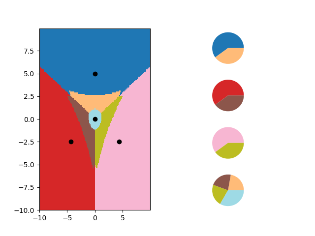
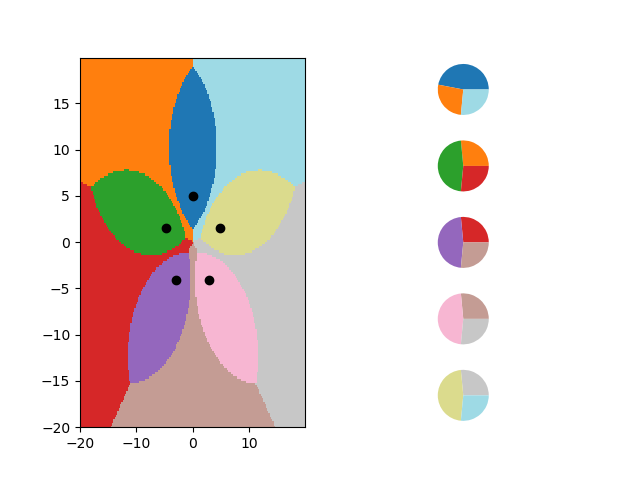
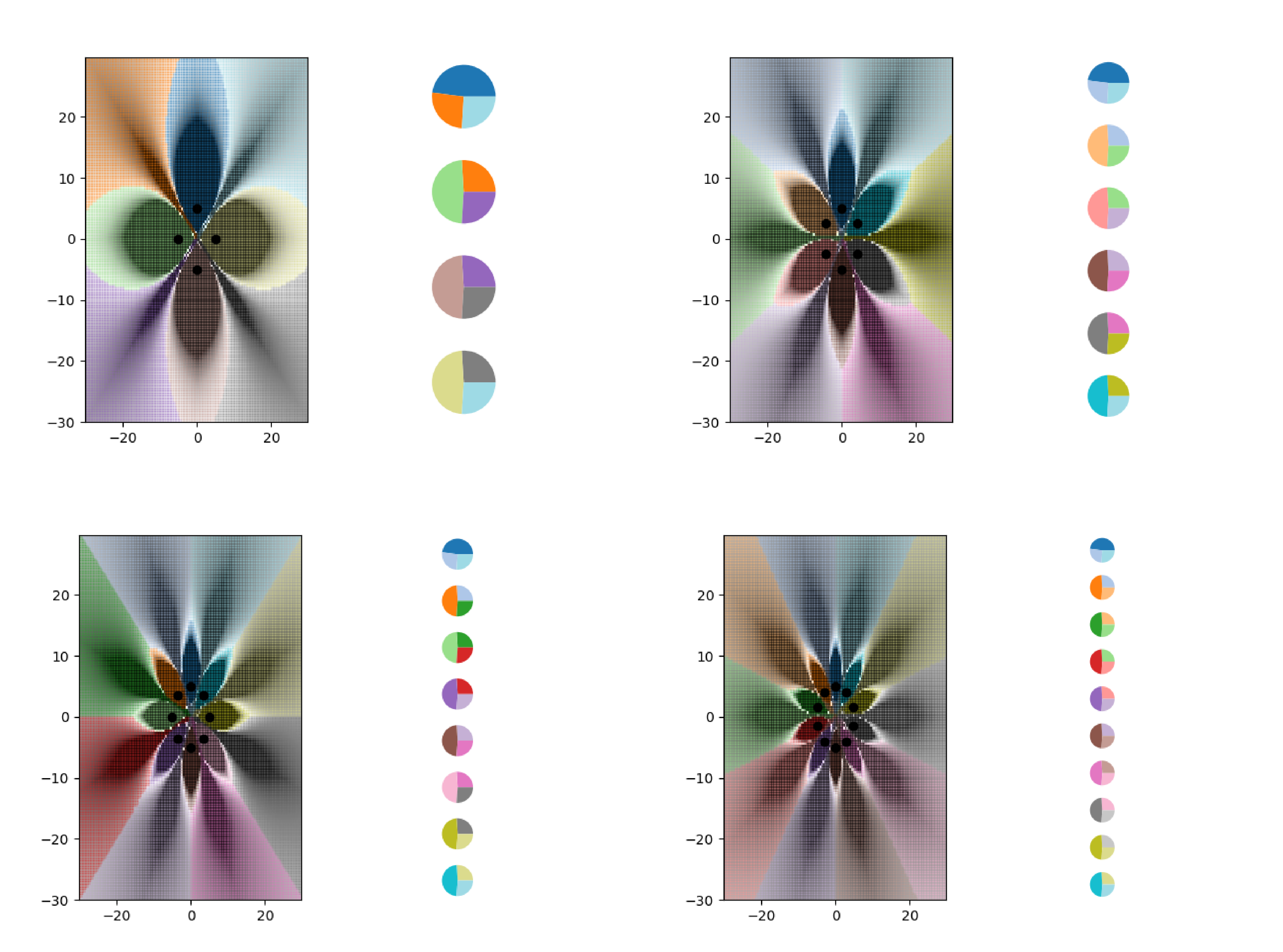
One way to select such labels is to use the same labels for each pair as in Theorem 1, This results in each having a label distribution containing two non-zero values: (associated with its main class) and (associated with the class created between itself and ). Meanwhile, contains one element with value (associated with its own class) and M-1 elements with value (each associated with a unique class created between and each one of the other points). To get probabilistic labels, we can normalize to instead have values and . The resulting decision landscape is visualized in Figure 3. The local decision boundaries in the neighbourhood between and any one of the surrounding prototypes then takes the following form.
| (2) |
Examining the asymptotic behavior as the total number of classes increases, we notice a potentially undesirable property of this configuration. Increases in ‘dilute’ classes and , which results in them shrinking towards . In the limit, only class remains. It is possible to find a configuration of probabilistic labels that results in asymptotically stable classes but this would require either lifting our previous restriction that the third label value be zero when separating three classes with two points, or changing the underlying geometrical arrangement of our prototypes.
Proposition 4.
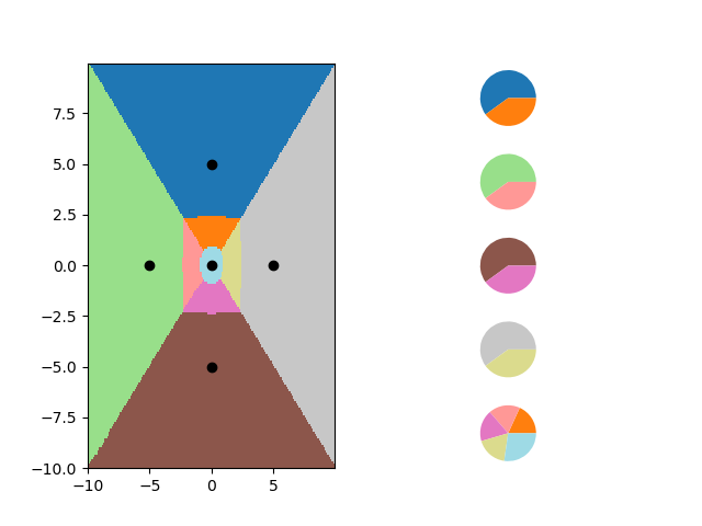
Suppose soft-label prototypes are arranged as the vertices of an -sided regular polygon. There exist soft labels such that fitting SLaPkNN with will divide the space into classes.
In this configuration, it is possible to decouple the system from the number of pairs that each prototype participates in. It can then be shown that the local decision boundaries, in the neighbourhood of any pair of adjacent prototypes, do not depend on M.
| (3) |
We visualize the resulting decision landscape in Figure 4.
By combining these two results, we can produce configurations that further increase the number of classes that can be separated by soft-label prototypes.
Theorem 5.
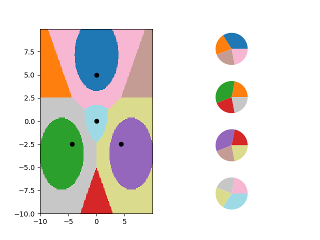
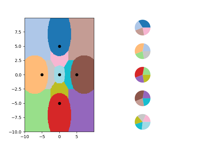
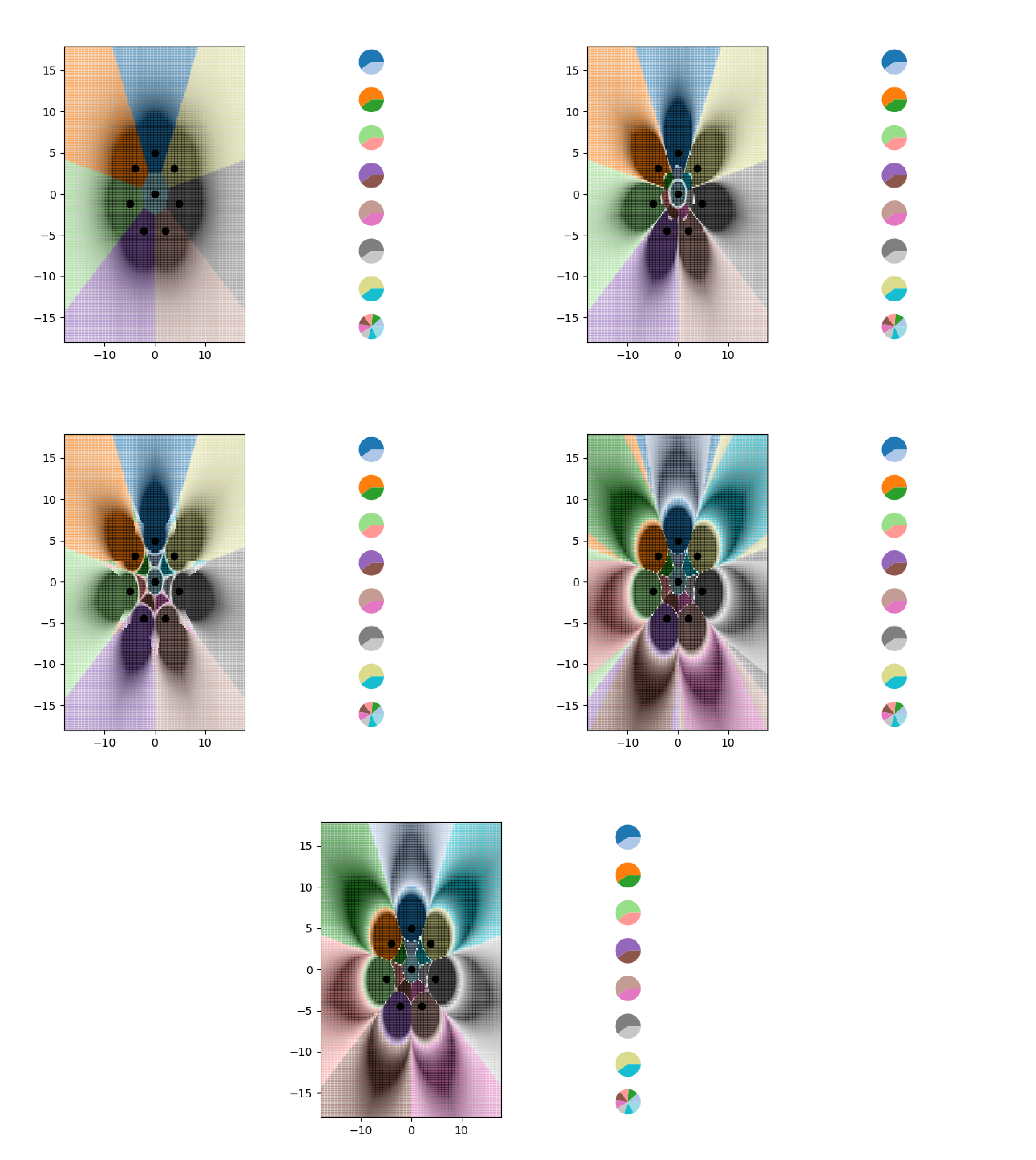
Suppose soft-label prototypes are arranged as the vertices and center of an -sided regular polygon. There exist soft labels such that fitting SLaPkNN with will divide the space into classes.
Interval Partitioning Methods
We now aim to show that two points can even induce multiple classes between them.
Lemma 6.
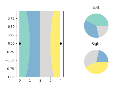
Assume that two points are positioned 4 units apart in two-dimensional Euclidean space. Without loss of generality, suppose that point and point have probabilistic labels and respectively. We denote the element of each label by and . There exist values of and such that SLaPkNN with can separate four classes when fitted on and .
We can again find a solution to this system that has symmetrical labels and also sets an element of the label to zero.
We visualize the results of fitting a SLaPkNN classifier with to a set of two points with these labels in Figure 6.
We can further extend this line of reasoning to produce the main theorem of this paper.
Theorem 7.
(Main Theorem) SLaPkNN with can separate classes using two soft-label prototypes.
This unexpected result is crucial for enabling extreme LO-shot learning as it shows that in some cases we can completely disconnect the number of classes from the number of prototypes required to separate them. The full proof can be found in the supplemental materials, but we provide a system of equations describing soft labels that result in two soft-label prototypes separating classes.
Other Results
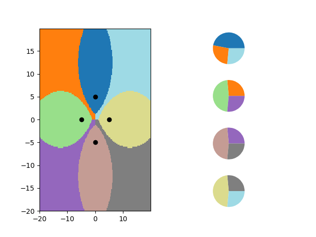
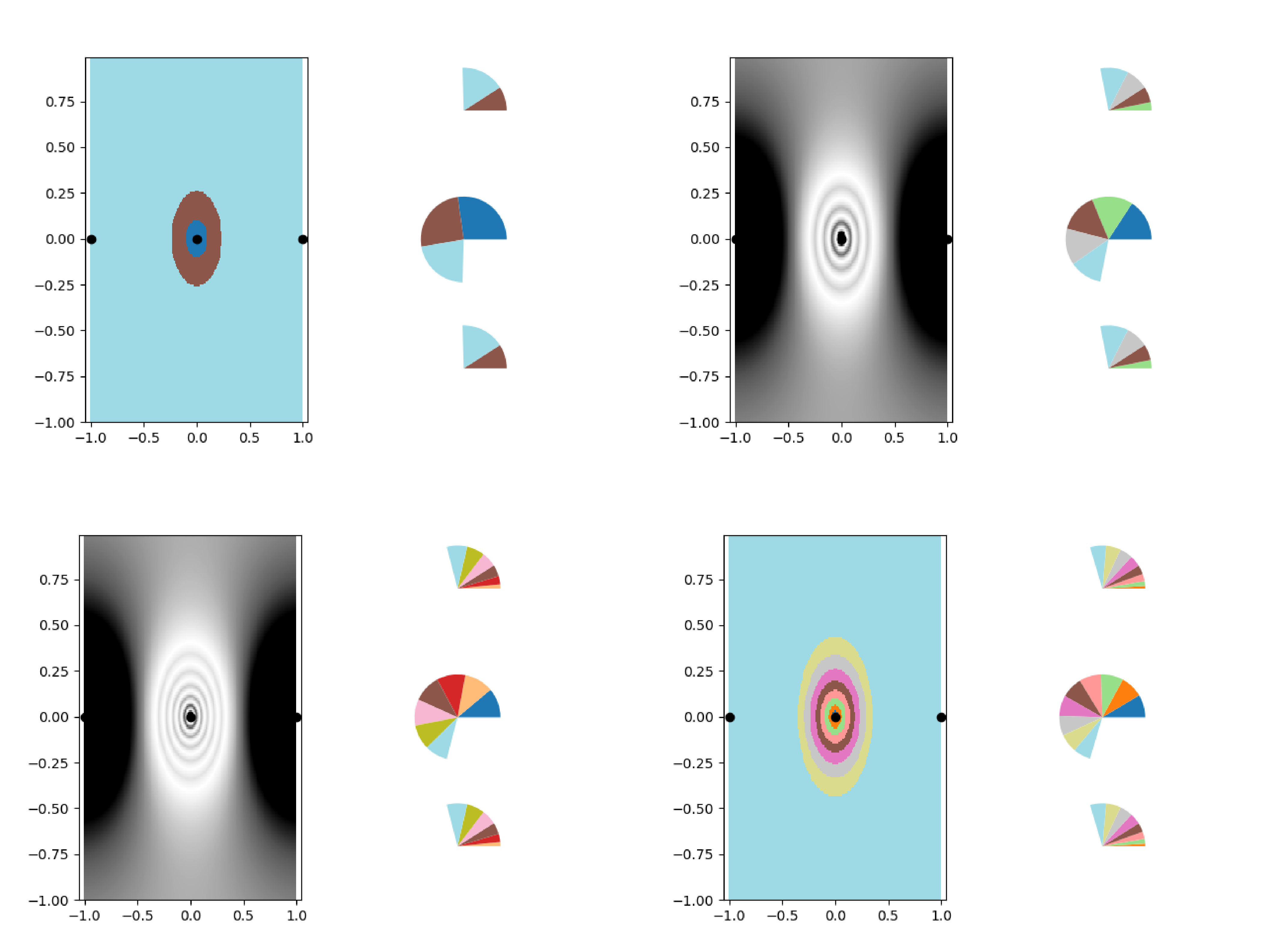
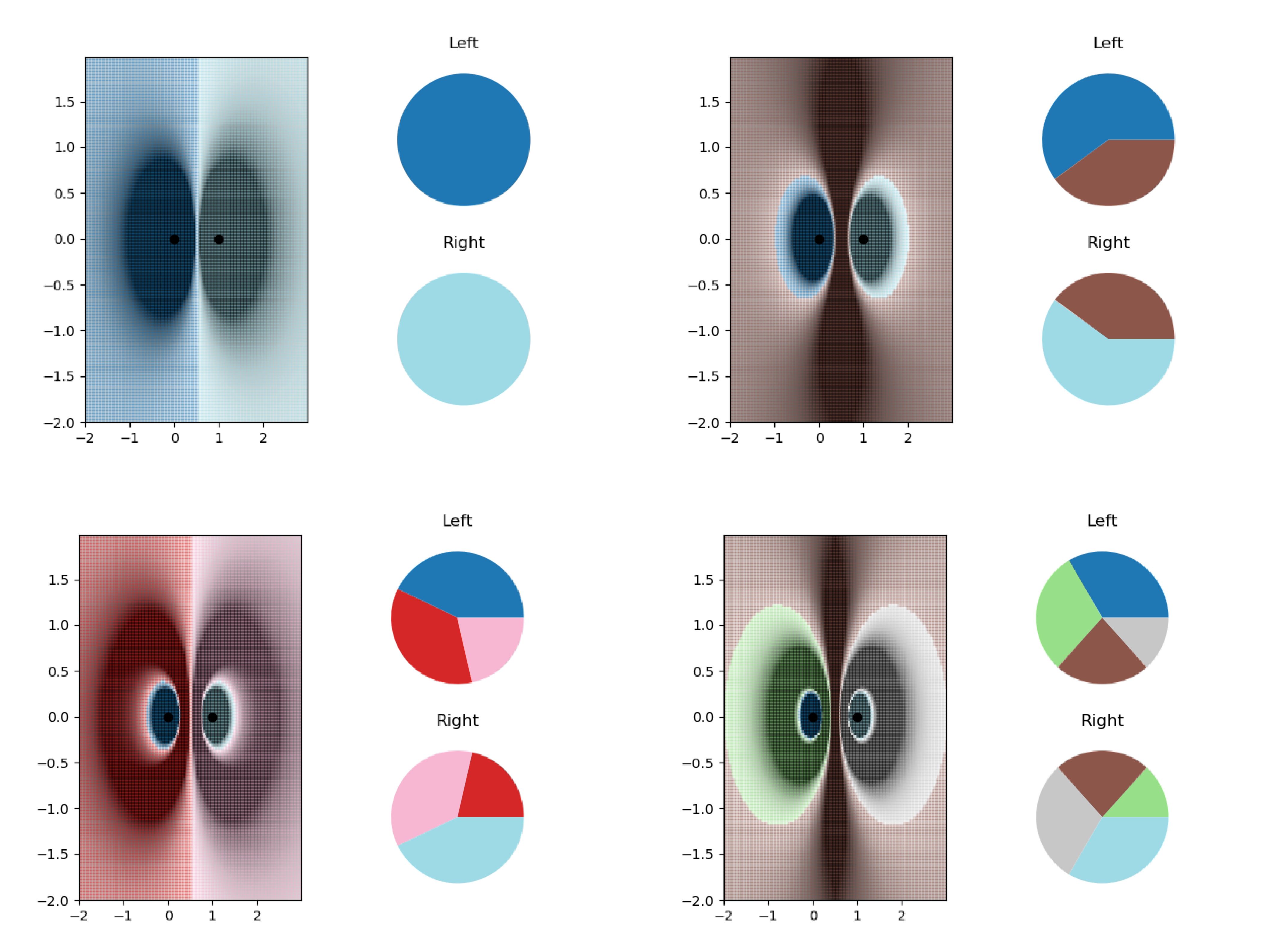
The diverse decision landscapes we have already seen were generated using probabilistic labels and . Using unrestricted soft labels and modifying enables us to explore a much larger space of decision landscapes. Due to space constraints we present only a few of the results from our experiments with modifying these parameters, but more are included in the accompanying supplemental material. One unexpected result is that SLaPkNN can generate any number of concentric elliptical decision bounds using a fixed number of prototypes as seen in Figures 7(a) and 7(b). In Figure 7(d), we show that variations in can cause large changes in the decision landscape, even producing non-contiguous classes.
Robustness
In order to understand the robustness of LO-shot learning landscapes to noise, we aim to analyze which regions are at highest risk of changing their assigned class if the prototype positions or labels are perturbed. We use the difference between the largest predicted label value and second-largest predicted label value as a measure of confidence in our prediction for a given point. The risk of a given point being re-classified is inversely proportional to the confidence. Since our aim is to inspect the entire landscape at once, rather than individual points, we visualize risk as a gradient from black (high confidence/low risk) to white (low confidence/high risk) over the space. We find that due to the inverse distance weighting mechanism, there are often extremely high confidence regions directly surrounding the prototypes, resulting in a very long-tailed, right-skewed distribution of confidence values. As a result, we need to either clip values or convert them to a logarithmic scale in order to be able to properly visualize them. We generally find that clipping is helpful for understanding intra-class changes in risk, while the log scale is more suited for visualizing inter-class changes in risk that occur at decision boundaries.
Figure 7 visualizes the risk gradient for many of the decision landscapes derived above. Overall, we find that LO-shot learning landscapes have lower risk in regions that are distant from decision boundaries and lowest risk near the prototypes themselves. Changes in can have a large effect on the inter-class risk behaviour which can be seen as changes in the decision boundaries. However, they tend to have a smaller effect on intra-class behavior in regions close to the prototypes. The most noticeable changes occur when increasing from 1 to 2, as this causes a large effect on the decision landscape itself, and from 2 to 3, which tends to not affect the decision landscape but causes a sharp increase in risk at decision boundaries. Meanwhile, increasing the number of classes () can in some cases cause large changes in the intra-class risk behaviour, but we can design prototype configurations (such as the ellipse generating configuration) that prevent this behaviour. In general, it appears that by tuning the prototype positions and labels we can simultaneously elicit desired properties both in the decision landscape and risk gradient. This suggests that LO-shot learning is not only feasible, but can also be made at least partially robust to noisy training data.
Case Study: Prototype Generation for Circles
We consider a simple example that captures the difference between hard and soft-label prototype generation. Assume that our data consists of concentric circles, where each circle is associated with a different class. We wish to select or generate the minimal number of prototypes such that the associated kNN classification rule will separate each circle as a different class. We tested several hard-label prototype methods and found their performance to be poor on this simulated data. Many of the methods produced prototypes that did not achieve separation between classes which prevents us from performing a fair comparison between hard and soft-label prototypes. In order to allow such a comparison, we analytically derive a near-optimal hard-label prototype configuration for fitting a 1NN classifier to the circle data.
Theorem 8.
Suppose we have concentric circles with radius for the circle. An upper bound for the minimum number of hard-label prototypes required for 1NN to produce decision boundaries that perfectly separate all circles, is ; with the circle requiring prototypes.
The proof can be found in the appendix. We can use the approximation to get that . Thus the upper bound for the minimum number of prototypes required is approximately . Figure 8 visualizes the decision boundaries of a regular kNN that perfectly separates six concentric circles given prototypes for the circle. It is possible that the number of prototypes may be slightly reduced by carefully adjusting the prototype locations on adjacent circles to maximize the minimal distance between the prototype midpoints of one circle and the prototypes of neighboring circles.
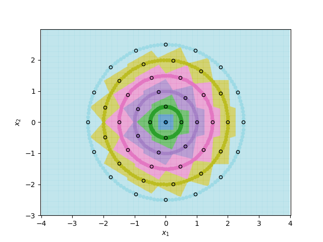
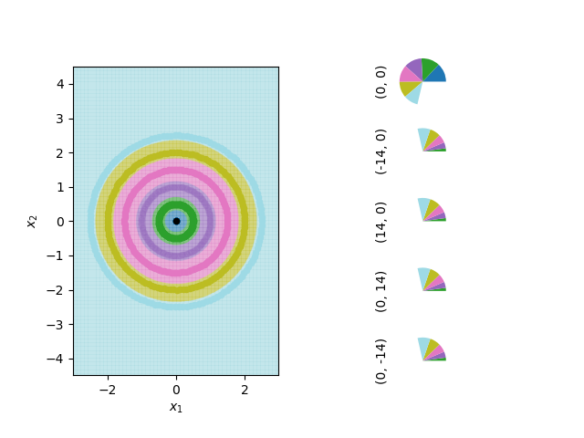
However, SLaPkNN requires only a constant number of prototypes to generate concentric ellipses. In Figure 9, SLaPkNN fitted on five soft-label prototypes is shown separating the six circles. The decision boundaries created by SLaPkNN match the underlying geometry of the data much more accurately than those created by 1NN. This is because 1NN can only create piecewise-linear decision boundaries.
In this case study, enabling soft labels reduced the minimal number of prototypes required to perfectly separate classes from down to . We note that the number of required hard-label prototypes may be reduced by carefully tuning as well as the neighbor weighting mechanism (e.g. uniform or distance-based). However, even in the best case, the number of required hard-label prototypes is at the very least linear in the number of classes.
Conclusion
We have presented a number of results that we believe can be used to create powerful and efficient dataset condensation and prototype generation techniques. More generally, our contributions lay the theoretical foundations necessary to establish ‘less than one’-shot learning as a viable new direction in machine learning research. We have shown that even a simple classifier like SLaPkNN can perform LO-shot learning, and we have proposed a way to analyze the robustness of the decision landscapes produced in this setting. We believe that creating a soft-label prototype generation algorithm that specifically optimizes prototypes for LO-shot learning is an important next step in exploring this area. Such an algorithm will also be helpful for empirically analyzing LO-shot learning in high-dimensional spaces where manually designing soft-label prototypes is not feasible.
Additionally, we are working on showing that LO-shot learning is compatible with a large variety of machine learning models. Improving prototype design is critical for speeding up instance-based, or lazy learning, algorithms like kNN by reducing the size of their training sets. However, eager learning models like deep neural networks would benefit more from the ability to learn directly from a small number of real samples to enable their usage in settings where little training data is available. This remains a major open challenge in LO-shot learning.
References
- Angelova, Abu-Mostafam, and Perona (2005) Angelova, A.; Abu-Mostafam, Y.; and Perona, P. 2005. Pruning training sets for learning of object categories. In 2005 IEEE Computer Society Conference on Computer Vision and Pattern Recognition, volume 1, 494–501. IEEE.
- Bachem, Lucic, and Krause (2017) Bachem, O.; Lucic, M.; and Krause, A. 2017. Practical coreset constructions for machine learning. arXiv preprint arXiv:1703.06476 .
- Bezdek and Kuncheva (2001) Bezdek, J. C.; and Kuncheva, L. I. 2001. Nearest prototype classifier designs: An experimental study. International Journal of Intelligent Systems 16(12): 1445–1473.
- Cohn, Ghahramani, and Jordan (1996) Cohn, D. A.; Ghahramani, Z.; and Jordan, M. I. 1996. Active learning with statistical models. Journal of Artificial Intelligence Research 4: 129–145.
- Dudani (1976) Dudani, S. A. 1976. The distance-weighted k-nearest-neighbor rule. IEEE Transactions on Systems, Man, and Cybernetics (4): 325–327.
- El Gayar, Schwenker, and Palm (2006) El Gayar, N.; Schwenker, F.; and Palm, G. 2006. A study of the robustness of KNN classifiers trained using soft labels. In IAPR Workshop on Artificial Neural Networks in Pattern Recognition, 67–80. Springer.
- El-Zahhar and El-Gayar (2010) El-Zahhar, M. M.; and El-Gayar, N. F. 2010. A semi-supervised learning approach for soft labeled data. In 2010 10th International Conference on Intelligent Systems Design and Applications, 1136–1141. IEEE.
- Fei-Fei, Fergus, and Perona (2006) Fei-Fei, L.; Fergus, R.; and Perona, P. 2006. One-shot learning of object categories. IEEE Transactions on Pattern Analysis and Machine Intelligence 28(4): 594–611.
- Garcia et al. (2012) Garcia, S.; Derrac, J.; Cano, J.; and Herrera, F. 2012. Prototype selection for nearest neighbor classification: Taxonomy and empirical study. IEEE Transactions on Pattern Analysis and Machine Intelligence 34(3): 417–435.
- Gou et al. (2012) Gou, J.; Du, L.; Zhang, Y.; Xiong, T.; et al. 2012. A new distance-weighted k-nearest neighbor classifier. Journal of Information and Computational Science 9(6): 1429–1436.
- Gweon, Schonlau, and Steiner (2019) Gweon, H.; Schonlau, M.; and Steiner, S. H. 2019. The k conditional nearest neighbor algorithm for classification and class probability estimation. PeerJ Computer Science 5: e194.
- Kanjanatarakul, Kuson, and Denoeux (2018) Kanjanatarakul, O.; Kuson, S.; and Denoeux, T. 2018. An evidential K-nearest neighbor classifier based on contextual discounting and likelihood maximization. In International Conference on Belief Functions, 155–162. Springer.
- Kusner et al. (2014) Kusner, M.; Tyree, S.; Weinberger, K.; and Agrawal, K. 2014. Stochastic neighbor compression. In International Conference on Machine Learning, 622–630.
- Lake, Salakhutdinov, and Tenenbaum (2015) Lake, B. M.; Salakhutdinov, R.; and Tenenbaum, J. B. 2015. Human-level concept learning through probabilistic program induction. Science 350(6266): 1332–1338.
- Macleod, Luk, and Titterington (1987) Macleod, J. E.; Luk, A.; and Titterington, D. M. 1987. A re-examination of the distance-weighted k-nearest neighbor classification rule. IEEE Transactions on Systems, Man, and Cybernetics 17(4): 689–696.
- Mitchell and Schaefer (2001) Mitchell, H.; and Schaefer, P. 2001. A “soft” K-nearest neighbor voting scheme. International Journal of Intelligent Systems 16(4): 459–468.
- Ruta (2006) Ruta, D. 2006. Dynamic data condensation for classification. In International Conference on Artificial Intelligence and Soft Computing, 672–681. Springer.
- Sener and Savarese (2017) Sener, O.; and Savarese, S. 2017. Active learning for convolutional neural networks: A core-set approach. arXiv preprint arXiv:1708.00489 .
- Shepard (1968) Shepard, D. 1968. A two-dimensional interpolation function for irregularly-spaced data. In Proceedings of the 1968 23rd ACM National Conference, 517–524.
- Snell, Swersky, and Zemel (2017) Snell, J.; Swersky, K.; and Zemel, R. 2017. Prototypical networks for few-shot learning. In Advances in Neural Information Processing Systems, 4077–4087.
- Sucholutsky and Schonlau (2019) Sucholutsky, I.; and Schonlau, M. 2019. Soft-Label Dataset Distillation and Text Dataset Distillation. arXiv preprint arXiv:1910.02551 .
- Sun, Qiao, and Cheng (2016) Sun, W. W.; Qiao, X.; and Cheng, G. 2016. Stabilized nearest neighbor classifier and its statistical properties. Journal of the American Statistical Association 111(515): 1254–1265.
- Thiel (2008) Thiel, C. 2008. Classification on soft labels is robust against label noise. In International Conference on Knowledge-Based and Intelligent Information and Engineering Systems, 65–73. Springer.
- Tong and Koller (2001) Tong, S.; and Koller, D. 2001. Support vector machine active learning with applications to text classification. Journal of Machine Learning Research 2(Nov): 45–66.
- Triguero et al. (2011) Triguero, I.; Derrac, J.; Garcia, S.; and Herrera, F. 2011. A taxonomy and experimental study on prototype generation for nearest neighbor classification. IEEE Transactions on Systems, Man, and Cybernetics, Part C (Applications and Reviews) 42(1): 86–100.
- Tsang, Kwok, and Cheung (2005) Tsang, I. W.; Kwok, J. T.; and Cheung, P.-M. 2005. Core vector machines: Fast SVM training on very large data sets. Journal of Machine Learning Research 6(Apr): 363–392.
- Vinyals et al. (2016) Vinyals, O.; Blundell, C.; Lillicrap, T.; Wierstra, D.; et al. 2016. Matching networks for one shot learning. In Advances in Neural Information Processing Systems, 3630–3638.
- Wang and Zhang (2019) Wang, S.; and Zhang, L. 2019. Regularized Deep Transfer Learning: When CNN Meets kNN. IEEE Transactions on Circuits and Systems II: Express Briefs .
- Wang et al. (2018) Wang, T.; Zhu, J.-Y.; Torralba, A.; and Efros, A. A. 2018. Dataset distillation. arXiv preprint arXiv:1811.10959 .
- Wang et al. (2020) Wang, Y.; Yao, Q.; Kwok, J. T.; and Ni, L. M. 2020. Generalizing from a few examples: A survey on few-shot learning. ACM Computing Surveys (CSUR) 53(3): 1–34.
- Yigit (2015) Yigit, H. 2015. ABC-based distance-weighted kNN algorithm. Journal of Experimental & Theoretical Artificial Intelligence 27(2): 189–198.