On SkipGram Word Embedding Models with Negative Sampling:
Unified Framework and Impact of Noise Distributions

Abstract

SkipGram word embedding models with negative sampling, or SGN in short, is an elegant family of word embedding models. In this paper, we formulate a framework for word embedding, referred to as Word-Context Classification (WCC), that generalizes SGN to a wide family of models. The framework, utilizing some “noise examples”, is justified through a theoretical analysis. The impact of noise distribution on the learning of the WCC embedding models is studied experimentally, suggesting that the best noise distribution is in fact the data distribution, in terms of both the embedding performance and the speed of convergence during training. Along our way, we discover several novel embedding models that outperform the existing WCC models.

1 Introduction

Learning the representations of words, or word embeddings (Mikolov et al., 2013a), is an important task in natural language processing (NLP).The advances of word embedding models (Pennington, Socher, and Manning, 2014; Peters et al., 2018; Devlin et al., 2019; Yang et al., 2019; Brown et al., 2020) have enabled numerous successes in NLP applications. In the past years, when building a machine learning model for NLP, starting from a pretrained word embedding has become a nearly standard practice.

The SkipGram models are among the first word-embedding models and have been widely used since their introduction. In a SkipGram model, the corpus is first parsed into a collection of (word, context) pairs, where the “context” is also a word living in a neighbourhood surrounding the “word” (often referred to as the “center word”). Then a predictor of the context from the center word is learned. The predictor is parameterized by the word embeddings, and learning the predictor gives the word embeddings.

Learning a SkipGram model may incur significant training complexity when the word vocabulary is large (since the predictor is a $V$-class classifier with large $V$). An elegant approach to by-pass this complexity is through “negative sampling”. In this approach, a set of word-context pairs are drawn from a “noise” distribution, under which the context is independent of the center word. These “noise pairs”, or “negative examples”, together with the word-context pairs from the corpus, or the “positive examples”, are then used to train a binary classifier that is parameterized by the word embeddings. In particular, the classifier is parameterized by the word embeddings and when the classifier is learned, one obtains the word embeddings. This “SkipGram with negative sampling” model is denoted by SGN in this paper for simplicity.

Despite its simplicity, SGN is shown to perform quite well in Mikolov et al. (2013b). Even though SGN now tends to be replaced by more sophisticated embedding models in NLP applications, to us, SGN is still a fundamental model: its elegance seems to imply a general principle for representation learning; its simplicity may allow a theoretical analysis. In contrast, in those more advanced and sophisticated models, e.g., BERT (Devlin et al., 2019), the design is primarily motivated by conceptual intuitions; theoretical analysis appears very difficult, at least with current analytic tools developed for deep learning.

But theoretical analysis of SGN remains thin to date. The main analytic result derived for SGN to date is that of Levy and Goldberg (2014). The result states that under a particular noise distribution, SGN can be interpreted as an implicit factorization of a point-wise mutual information matrix.

Many questions in fact are unanswered for SGN. Specifically, in this paper, we ask the following questions. Beyond that particular distribution, if one chooses a different noise distribution, is SGN still theoretically justified? Is there a general principle underlying SGN that allows us to build new embedding models? If so, how does the noise distribution impact the training of such models and their achievable performances? These questions are answered in this paper.

To that end, we formalize a unified framework, referred to as “word-context classification” or WCC, for SGN-like word embedding models. The framework, including SGN as a special case, allows the noise distribution to take arbitrary forms and hence results in broad family of SGN-like models. We also provide a theoretical analysis that justifies the WCC framework. Consequently, the matrix-factorization result of Levy and Goldberg (2014) can also be derived from this analysis as a special case.

In addition, the impact of noise distribution on learning word embeddings in WCC is also studied in this paper. For this purpose, we classify WCC models into the conventional SGN models and the conditional SGN models, according to the factorization form of the noise distribution. We argue theoretically that the conditional models are inherently advantageous, thereby hypothesizing that the best WCC model is in fact the conditional SGN model with noise distribution precisely equal to the data distribution, i.e., the word-context pair distribution in the corpus. It is unfortunate however that the conditional models are in fact discouraged due to their high training complexity. To tackle this, we propose a variant of the conditional SGN models, the adaptive conditional SGN (caSGN) models, where the noise distribution adapts itself gradually towards the data distribution. Such an adaptation achieved by modeling the noise distribution generatively and learning the generator in a way similar to GAN (Goodfellow et al., 2014). We show that the caSGN models may be constructed with various structures of the generator. In particular, a previously proposed model, ACE (Bose, Ling, and Cao, 2018), may be regarded as a special form of caSGN. For the sake of comparison, the adaptive version of the unconditional SGN model is also presented.

Extensive experiments are then conducted to further this study. A wide spectrum of WCC models (SGN, versions of caSGN, and ACE) are implemented and compared to investigate the impact of noise distribution. These learned embeddings are evaluated using three downstream tasks over twelve datasets. Our experimental results suggest that indeed the caSGN models outperform other models, validating the validity of the WCC framework and confirming the hypothesis that the best noise distribution in WCC is in fact the data distribution.

2 Related Work

There have been a number of recent efforts to improve negative sampling in the word embedding learning. Zhang and Zweigenbaum (2018) designed a fixed conditional negative sampler, but the complexity of sampling is proportional to the size of the vocabulary. Hence to reduce time complexity, the authors pre-computed the noise distribution off-line for each center word and restricted the vocabulary size as $10k$ in their experiments. Both Chen et al. (2018) and Guo et al. (2018) designed a dynamic sampler that selects negative words by ranking score. Specifically, they mended the negative sampling strategy from the optimization perspective. In addition, there are some other works regarding revising negative sampling (Sun et al., 2016; Soleimani and Matwin, 2018; Mu, Yang, and Zheng, 2019), but they focus on designing new objective functions and are not directly related to our paper.

GAN-based negative sampler has also been used in other lines of NLP research (Wang, Liu, and Zhao, 2017; Wang et al., 2017; Wang, Li, and Pan, 2018; Dai et al., 2019; Budhkar et al., 2019). For example, Wang, Li, and Pan (2018) employed GAN-based framework on knowledge representation learning and Budhkar et al. (2019) imposed GAN-based method to generate natural language.

It is worth noting that the well-known unsupervised learning framework, noise constrastive estimation or NCE (Gutmann and Hyvärinen, 2012), adopts a similar negative-sampling approach. Indeed, some previous work has suggested that negative sampling and NCE are very close to each other when applied to the same model (Melamud, Dagan, and Goldberger, 2017; Labeau and Allauzen, 2018; Ma and Collins, 2018). However, the connection between the two is rather loose here. In particular, SGN and more broadly WCC can not be justified using NCE in the sense that in NCE it is required that one can evaluate the noise distribution, whereas in WCC this is not required.

3 Word-Context Classification

3.1 The Word Embedding Problem

Let ${\cal X}$ denote a vocabulary of words, and let ${\cal Y}$ denote a set of contexts. When considering the SkipGram models, context is often considered as a single word, which is the case ${\cal Y}$ is ${\cal X}$. But to better distinguish words and contexts, we prefer using ${\cal Y}$ to denote the set of all contexts.

In this setting, a given training corpus may be parsed into a collection ${\cal D}^{+}$ of word-context pairs $(x,y)$ from ${\cal X}\times{\cal Y}$. For example, as is standard (Mikolov et al., 2013b), we may use a running window of length $2L+1$ to slide over the corpus; for each window location, we collect $2L$ word-context pairs, where the word located at the center of the window is taken as $x$ in each $(x,y)$ pair, and each of the remaining $2L$ words in the window is taken as a context $y$, paired with $x$. This gives rise to the training data, or the positive sample ${\cal D}^{+}$. With respect to the context $y$, we sometimes call the word $x$ the “center word”.

As is conventional, the word-context pairs ${\cal D}^{+}$ are assumed to contain i.i.d. instances of a random word-context pair $(X,Y)$ drawn from an unknown distribution ${\mathbb{P}}$ on ${\cal X}\times{\cal Y}$. We will use ${\mathbb{P}}_{\cal X}$ to denote the marginal of ${\mathbb{P}}$ on ${\cal X}$, and for each $x\in{\cal X}$, use ${\mathbb{P}}_{{\cal Y}|{x}}$ to denote the conditional distribution of $Y$ given $X=x$ under ${\mathbb{P}}$. Let $N^{+}$ denote the number of pairs in ${\cal D}^{+}$.

The objective of word embedding is to learn a vector representation for each word in ${\cal X}$ (and possibly also for each context in ${\cal Y}$).

We now introduce the Word-Context Classification (WCC) framework, which provides a unified perspective to negative-sampling based SkipGram embedding models.

3.2 The WCC Framework

For each $x\in{\cal X}$, we let ${\mathbb{Q}}_{{\cal Y}|x}$ be a distribution on ${\cal Y}$, and we define a distribution ${\mathbb{Q}}$ on ${\cal X}\times{\cal Y}$ as the noise distribution. Given ${\mathbb{Q}}$, we draw $N^{-}$ word-context pairs i.i.d. from ${\mathbb{Q}}$ to form a noise sample or negative sample ${\cal D}^{-}$.

Now we define a binary classification problem on samples ${\cal D}^{+}$ and ${\cal D}^{-}$ with the objective of learning a binary classifier capable of distinguishing the word-context pairs drawn from ${\mathbb{P}}$ from those drawn from ${\mathbb{Q}}$. The word embedding problem of interest will be nested inside the classifier-learning problem.

To that end, let binary variable $U$ denote the class label associated with each word-context pair $(X,Y)$. Specifically, whenever we draw a pair $(X,Y)$ from ${\mathbb{P}}$, we also create a label $U\!=\!1$, and likewise, whenever we draw a pair $(X,Y)$ from ${\mathbb{Q}}$, we also create a label $U\!=\!0$. That is, all pairs in ${\cal D}^{+}$ are associated with label $U\!=\!1$, and all pairs in ${\cal D}^{-}$ associated with label $U\!=\!0$. Then the classification problem is equivalent to learning the conditional distribution $p_{U|XY}(\cdot|x,y)$ from ${\cal D}^{+}$ and ${\cal D}^{-}$.

Let $\sigma(\cdot)$ denote the logistic function and let the classifier $p_{U|XY}(\cdot|x,y)$ take the form

$$p_{U|XY}(1|x,y):=\sigma\left(s(x,y)\right)$$ (1)

for some function $s$ on ${\cal X}\times{\cal Y}$. Note that such form of classifiers is well known to be sufficiently expressive and entail no loss of generality (Jordan, 1995). We will refer to $s(x,y)$ as the score of word-context pair $(x,y)$. Any parameterized modelling for such classification problem then reduces to a selection of the score function $s(\cdot)$.

In order to learn a distributed representation of words, consider the following family of parameterization of the score function $s$.

Let $\overline{\cal X}$ and $\overline{\cal Y}$ be two vector spaces, serving as the embedding spaces for words and contexts respectively. Let $f:{\cal X}\rightarrow\overline{\cal X}$ and $g:{\cal Y}\rightarrow\overline{\cal Y}$ be two functions representing the embedding maps for words and contexts. Let $s(x,y)$ take the form

$$s(x,y):={\bf score}\left(f(x),g(y)\right),$$ (2)

for some function ${\bf score}(\cdot)$ on $\overline{\cal X}\times\overline{\cal Y}$. In the most general case, the functions $f$, $g$ and ${\bf score}$ can all be made learnable. In this paper, we however follow the classical choice in Mikolov et al. (2013b) for simplicity, where $\overline{\cal X}$ and $\overline{\cal Y}$ are taken as the same vector space, and the function ${\bf score}(\cdot)$ is taken as standard inner product operation therein, namely not to be learned.

It is easy to see that the standard cross-entropy loss for this classification problem is

$$\ell\!\!=\!-\!\!\!\!\!\sum_{(x,y)\in{\cal D}^{+}}\!\!\!\!\!\ \log\sigma\left(s(x,y)\right)-\!\!\!\!\!\sum_{(x,y)\in{\cal D}^{-}}\!\!\!\!\!\ \log\sigma\left(-s(x,y)\right).$$ (3)

The standard Maximum Likelihood formulation of the learning problem is then minimizing the loss function $\ell$ over all possible embedding maps $f$ and $g$, namely, solving for

$$\left({f^{*}},{g^{*}}\right):=\arg\min_{f,g}\ell(f,g).$$ (4)

Above we have explicitly written the cross-entropy loss $\ell$ as a function of the embedding maps $f$ and $g$.

At this end, we see that solving this binary “word-context classification” problem provides an embedding map $f$, thus giving a solution to the word embedding problem of interest. We refer to this framework as the Word-Context Classification or WCC framework.

3.3 Theoretical Properties of WCC

To justify the WCC framework, we derive a set of theoretical properties for the optimization problem in (4).

Let $\widetilde{\mathbb{P}}$ and $\widetilde{\mathbb{Q}}$ be the empirical word-context distributions observed in ${\cal D}^{+}$ and ${\cal D}^{-}$ respectively. That is, $\widetilde{\mathbb{P}}(x,y)=\frac{\#(x,y)}{N^{+}}$ where $\#(x,y)$ is the number of times the word-context pair $(x,y)$ appears in ${\cal D}^{+}$, and $\widetilde{\mathbb{Q}}(x,y)$ is defined similarly.

We will say that the distribution $\widetilde{\mathbb{Q}}$ covers the distribution $\widetilde{\mathbb{P}}$ if the support ${\rm Supp}\left(\widetilde{\mathbb{P}}\right)$ of $\widetilde{\mathbb{P}}$ is a subset of the support ${\rm Supp}\left(\widetilde{\mathbb{Q}}\right)$ of $\widetilde{\mathbb{Q}}$. Recall that the support of a distribution is a set of all points on which the probability is non-zero.

Note that the function $s$ assigns a score to each word-context pair $(x,y)$. Thus we can view $s$ as an $|{\cal X}|\times|{\cal Y}|$ “score matrix”. Additionally, the loss $\ell$ in (3) may also be treated as a function of matrix $s$.

Theorem 1.

Suppose that $\widetilde{\mathbb{Q}}$ covers $\widetilde{\mathbb{P}}$. Then the following holds.

1. The loss $\ell$, as a function of $s$, is convex in $s$.

2. If $f$ and $g$ are sufficiently expressive, then there is a unique configuration $s^{*}$ of $s$ that minimizes $\ell(s)$, and the global minimizer $s^{*}$ of $\ell(s)$ is given by

   $$s^{*}(x,y)=\log\frac{\widetilde{\mathbb{P}}(x,y)}{\widetilde{\mathbb{Q}}(x,y)}+\log\frac{N^{+}}{N^{-}}$$

   for every $(x,y)\in{\cal X}\times{\cal Y}$.

Proof.

The first part is straightforward by computing the second derivative:

$$\frac{\partial^{2}\left(-\log\sigma(s)\right)}{\partial s^{2}}=\frac{\partial\left(\sigma(s)-1\right)}{\partial s}=\sigma(s)\cdot\left(1-\sigma(s)\right)\geqslant 0.$$

Thus, $-\log\sigma\left(s\right)$ is a convex function in $s$, and we can prove $-\log\sigma\left(-s\right)$ is also a convex function following the same way. Since the summation of the convex functions is still a convex function, the loss $\ell$ is convex in $s$.

For the second part, we know that the size of ${\cal D}^{+}$ is ${N^{+}}\widetilde{\mathbb{P}}(x,y)$ and the size of ${\cal D}^{-}$ is ${N^{-}}\widetilde{\mathbb{Q}}(x,y)$. Hence the prior distribution of binary random variable $U$ is:

$$p_{U}(U=1)=\frac{{N^{+}}\widetilde{\mathbb{P}}(x,y)}{{N^{+}}\widetilde{\mathbb{P}}(x,y)+{N^{-}}\widetilde{\mathbb{Q}}(x,y)}.$$ (5)

Recall that

$$\ell-{\rm H}(p_{U})={\rm KL}(p_{U}||p_{U|XY}),$$

where ${\rm H}(p_{U})$ is the entropy of $p_{U}$ and ${\rm KL}(p_{U}||p_{U|XY})$ is the Kullback-Leibler divergence between $p_{U}$ and $p_{U|XY}$. Given ${N^{+}}$, ${N^{-}}$, $\widetilde{\mathbb{P}}(x,y)$ and $\widetilde{\mathbb{Q}}(x,y)$, ${\rm H}(p_{U})$ is a constant. In this case,

$$\min_{f,g}\ell(f,g)=\min_{f,g}{\rm KL}(p_{U}||p_{U|XY}).$$

Since ${\rm KL}(p_{U}||p_{U|XY})$ reaches the minimum value $0$ when $p_{U}=p_{U|XY}$, we let

$$p_{U}(U=1)=p_{U|XY}(1|x,y)\Longrightarrow\frac{{N^{+}}\widetilde{\mathbb{P}}(x,y)}{{N^{+}}\widetilde{\mathbb{P}}(x,y)+{N^{-}}\widetilde{\mathbb{Q}}(x,y)}=\sigma\left(s^{*}(x,y)\right),$$ (6)

which indicates $s^{*}(x,y)=\log\frac{\widetilde{\mathbb{P}}(x,y)}{\widetilde{\mathbb{Q}}(x,y)}+\log\frac{N^{+}}{N^{-}}$. We then know this is the unique solution due to the convexity. ∎

Note that the second statement of the theorem does not imply that there is a unique $\left({f^{*}},{g^{*}}\right)$ that minimizes $\ell(f,g)$. In fact there is a continuum of $\left({f^{*}},{g^{*}}\right)$’s which all minimize $\ell(f,g)$ equally well. A consequence of Theorem 1 is the following result.

Corollary 1.

Let $N^{+}=n$ and $N^{-}=kn$. Suppose that ${\mathbb{Q}}$ covers ${\mathbb{P}}$, and that $f$ and $g$ are sufficiently expressive. Then it is possible to construct a distribution $\widehat{\mathbb{P}}$ on ${\cal X}\times{\cal Y}$ using ${f^{*}},{g^{*}}$, $k$, and ${\mathbb{Q}}$ such that for every $(x,y)\in{\cal X}\times{\cal Y}$, $\widehat{\mathbb{P}}(x,y)$ converges to ${\mathbb{P}}(x,y)$ in probability as $n\rightarrow\infty$.

Proof.

Suppose ${f^{*}},{g^{*}}$, $k$, and ${\mathbb{Q}}$ are all known. Recall that $s^{*}(x,y)=\log\frac{\widetilde{\mathbb{P}}(x,y)}{\widetilde{\mathbb{Q}}(x,y)}-\log k$ and $s^{*}(x,y)=\langle f^{*}(x),g^{*}(y)\rangle$. We then reconstruct $\widehat{\mathbb{P}}$ as

$$\begin{split}\widehat{\mathbb{P}}(x,y)&=\underbrace{\exp\left\{\langle f^{*}(x),g^{*}(y)\rangle+\log k\right\}}_{A(x,y)}\cdot\mathbb{Q}(x,y)\\ &=A(x,y)\cdot\widetilde{\mathbb{Q}}(x,y)\cdot\frac{\mathbb{Q}(x,y)}{\widetilde{\mathbb{Q}}(x,y)}\\ &=\widetilde{\mathbb{P}}(x,y)\cdot\frac{\mathbb{Q}(x,y)}{\widetilde{\mathbb{Q}}(x,y)}\\ &=\mathbb{P}(x,y)\cdot\frac{\widetilde{\mathbb{P}}(x,y)}{\mathbb{P}(x,y)}\cdot\frac{\mathbb{Q}(x,y)}{\widetilde{\mathbb{Q}}(x,y)}.\end{split}$$ (7)

According to the weak law of large numbers, $\widetilde{\mathbb{P}}(x,y)$ converges to ${\mathbb{P}}(x,y)$ in probability as $n\rightarrow\infty$ and $\widetilde{\mathbb{Q}}(x,y)$ converges to ${\mathbb{Q}}(x,y)$ in probability as $n\rightarrow\infty$. Thus, for every $(x,y)\in{\cal X}\times{\cal Y}$, $\widehat{\mathbb{P}}(x,y)$ converges to ${\mathbb{P}}(x,y)$ in probability as $n\rightarrow\infty$ ∎

We note that Corollary 1 justifies the WCC framework, since under the condition of the corollary, one can reconstruct the unknown data distribution ${\mathbb{P}}$ from the learned embedding maps ${f^{*}}$ and ${g^{*}}$ without referring to the samples ${\cal D}^{+}$ and ${\cal D}^{-}$. That is, for sufficiently large sample sizes $N^{+}$ and $N^{-}$, the learned embedding maps ${f^{*}}$ and ${g^{*}}$ results in virtually no loss of the information contained in the data distribution ${\mathbb{P}}$.

There are other consequences of Theorem 1, which we postpone to discuss in a later section. For later use, we present another result.

Lemma 1.

The derivative of the loss function $\ell$ with respect to $s(x,y)$ is

$$\frac{\partial\ell}{\partial s(x,y)}\!\!=\!\!\sigma\left(s(x,y)\right)(N^{-}\widetilde{\mathbb{Q}}(x,y)-e^{-s(x,y)}N^{+}\widetilde{\mathbb{P}}(x,y)).$$

3.4 Different Forms of Noise Distribution ${\mathbb{Q}}$

From the formulation of WCC, it is apparent that the choice of the noise distribution ${\mathbb{Q}}$ has an effect on this classifier learning problem and possibly impact the quality and training of the word embeddings. We now discuss various options in selecting the noise distribution ${\mathbb{Q}}$, resulting in different versions of SkipGram models. Such models will all be referred to SGN models, for the ease of reference.

3.4.1 SGN Model

Let ${\mathbb{Q}}$ factorize in the following form

$${\mathbb{Q}}(x,y)=\widetilde{\mathbb{P}}_{\cal X}(x){\mathbb{Q}}_{\cal Y}(y).$$ (8)

In such a model, the noise context does not depend on the noise center word. Thus we may also refer to such a model as an unconditional SGN model. The standard SGN model of Mikolov et al. (2013b), which we will refer to as “Vanilla SGN”, can be regarded as unconditional SGN in which ${\mathbb{Q}}_{\cal Y}$ takes a particular form (see later).

The following result follows from Theorem 1.

Corollary 2.

In an unconditional SGN model, suppose that $f$ and $g$ are sufficiently expressive. Let $N^{+}\!\!\!=n$ and $N^{-}\!\!\!=kn$. Then the global minimizer of loss function (3) is given by

$$s^{*}(x,y)=\overline{x}\cdot\overline{y}=\log\frac{\widetilde{\mathbb{P}}(x,y)}{\widetilde{{\mathbb{P}}}_{\cal X}(x)\widetilde{{\mathbb{Q}}}_{\cal Y}(y)}-\log k.$$

As a special case of Corollary 2, when $\widetilde{{\mathbb{Q}}}_{\cal Y}=\widetilde{\mathbb{P}}_{\cal Y}$, the term $\log\frac{\widetilde{\mathbb{P}}(x,y)}{\widetilde{{\mathbb{P}}}_{\cal X}(x)\widetilde{{\mathbb{Q}}}_{\cal Y}(y)}$ is called “pointwise mutual information” (PMI) (Levy and Goldberg, 2014). In this case, the above corollary states that the WCC learning problem can be regarded as implicitly factorizing a “shifted PMI matrix”, recovering the well-known result of Levy and Goldberg (2014) on SkipGram word embedding models.

It is natural to consider the following forms of ${\mathbb{Q}}_{\cal Y}$ in unconditional SGN.

1. “uniform SGN” (ufSGN): Let ${\mathbb{Q}}_{\cal Y}$ be the discrete uniform distribution over ${\cal Y}$, i.e. ${\mathbb{Q}}_{\cal Y}(y)=1/{|{\cal Y}|}$.

2. “unigram SGN” (ugSGN): Let ${\mathbb{Q}}_{\cal Y}$ be empirical distribution ${\mathbb{P}}_{\cal Y}$ of context word in the corpus, that is, ${\mathbb{Q}}_{\cal Y}(y)=f_{y}/\sum_{y\in{\cal Y}}{f_{y}}$, where $f_{y}$ is the frequency at which the context word $y$ has occurred in the corpus.

3. “3/4-unigram SGN” (3/4-ugSGN): Let ${\mathbb{Q}}_{\cal Y}$ be defined by ${\mathbb{Q}}_{\cal Y}(y)=f_{y}^{3/4}/\sum_{y\in{\cal Y}}{f_{y}^{3/4}}$. This is precisely the noise distribution used in vanilla SGN (Mikolov et al., 2013b).

3.4.2 Conditional SGN

In this case, we factorize ${\mathbb{Q}}$ as

$${\mathbb{Q}}(x,y)=\widetilde{\mathbb{P}}_{\cal X}(x){\mathbb{Q}}_{{\cal Y}|x}(y),$$

where ${\mathbb{Q}}_{{\cal Y}|x}(\cdot)$ varies with $x$. Such form of ${\mathbb{Q}}$ includes all possible distributions ${\mathbb{Q}}$ whose marginals ${\mathbb{Q}}_{\cal X}$ on the center word are the same as $\widetilde{\mathbb{P}}_{\cal X}$. Specifically, if we take ${\mathbb{Q}}_{{\cal Y}|x}$ as $\widetilde{\mathbb{P}}_{{\cal Y}|x}$, then ${\mathbb{Q}}$ is $\widetilde{\mathbb{P}}$. Before we proceed, we make the following remark.

Remark 1. In Theorem 1 and Corollary 1, the WCC framework is justified for any choice of empirical noise distribution $\widetilde{\mathbb{Q}}$ that covers $\widetilde{\mathbb{P}}$. Consider some $(x,y)\in{\rm Supp}\left(\widetilde{\mathbb{Q}}\right)\setminus{\rm Supp}\left(\widetilde{\mathbb{P}}\right)$, namely, $(x,y)$ is “covered” by $\widetilde{\mathbb{Q}}$ but not by $\widetilde{\mathbb{P}}$. By Lemma 1, the gradient is

$$\frac{\partial\ell}{\partial s(x,y)} = \sigma\left(s(x,y)\right)\cdot N^{-}\widetilde{\mathbb{Q}}(x,y).$$

That is, the gradient signal contains only one term, which is used to update the representation $(f(x),g(y))$ for the pair $(x,y)$, which is outside the positive examples. Although the gradient signal updates the embedding $f(x)$, but the training is towards making the classifier sensitive to negative examples (make it to have low loss), without contributing to differentiating the negative examples from the positive one (namely, without aiming at reducing the loss for positive examples). Such a direction of training, not necessarily “wrong”, somewhat deviates from the training objective (i.e., reducing the loss for both positive and negative examples). In the case when the ${\rm Supp}\left(\widetilde{\mathbb{Q}}\right)$ of $\widetilde{\mathbb{Q}}$ contains the support ${\rm Supp}\left(\widetilde{\mathbb{P}}\right)$ of $\widetilde{\mathbb{P}}$ but is much larger, there are a significant fraction of such negative examples outside ${\rm Supp}\left(\widetilde{\mathbb{P}}\right)$. This may result in slow training.

Thus in the sense to efficiently learn word embeddings in the WCC framework, we have the following hypothesis:

Hypothesis 1.

The best $\widetilde{\mathbb{Q}}$ is the one that barely covers $\widetilde{\mathbb{P}}$, namely, equal to $\widetilde{\mathbb{P}}$.

Remark 2. It is important to note that in order to achieve better performance on some NLP downstream tasks, $\widetilde{\mathbb{Q}}$ should not be exactly $\widetilde{\mathbb{P}}$ during the whole training phase. This is because target words in these tasks may not frequently appear in the training corpus, and if they are rarely trained, the learned embeddings will not able to give a good performance. It turns out that we usually apply the sub-sampling technique and try to improve the entropy of $\widetilde{\mathbb{Q}}$ ( e.g., using “3/4-unigram" instead of “unigram" (Mikolov et al., 2013b) ) in practice.

Under this hypothesis, we wish to choose ${\mathbb{Q}}_{{\cal Y}|x}$ to be equal to, or at least to closely resemble, $\widetilde{\mathbb{P}}_{{\cal Y}|x}$.

This choice however entails nearly prohibitively high computation complexity for optimization using mini-batched SGD. This is because for each word-context pair in a mini-batch, the context word needs to be sampled from its own distribution $\widetilde{\mathbb{P}}_{{\cal Y}|x}$, depending on the center word $x$. Such a sampling scheme is not parallelizable within the mini-batch, under current deep learning libraries.

In the next subsection, we will present a solution that can bypass this complexity.

3.4.3 Conditional Adaptive SGN (caSGN)

Now we consider a version of $\left\{\widetilde{\mathbb{Q}}^{t}_{{\cal Y}|x}:x\in{\cal X}\right\}$ that varies with training iteration $t$. We consider training based on mini-batched SGD, where each batch is defined as a random collection of positive examples together with their corresponding negative examples (which are $k$ times many). We take $t$ as the index of a batch. Suppose training is such that the loss computed for a batch converges and that $\widetilde{\mathbb{Q}}^{t}_{{\cal Y}|x}$ converges to $\widetilde{\mathbb{P}}_{{\cal Y}|x}$ for each $x\in{\cal X}$. Let $T$ be the total number of training iterations (largest batch number). The empirical distribution, say $\widehat{\mathbb{Q}}^{T}$, of the noise word-context pair seen during the entire training process is then $\widehat{\mathbb{Q}}^{T}(x,y)\!\!=\!\!\sum\limits_{t=1}^{T}\widetilde{\mathbb{Q}}^{t}_{{\cal Y}|x}(y)\widetilde{\mathbb{P}}_{\cal X}(x)/T$. Under the above stated assumptions, it is easy to see that $\widehat{\mathbb{Q}}^{T}$ must converge to $\widetilde{\mathbb{P}}$ with increasing $T$. Thus, when $T$ is large enough, we can regard training as a version of mini-batched SGD with ${\mathbb{Q}}$ chosen as a distribution arbitrarily close to $\widetilde{\mathbb{P}}$, or a conditional SGN with ${\mathbb{Q}}_{{\cal Y}|x}$ arbitrarily close to $\widetilde{\mathbb{P}}_{{\cal Y}|x}$.

This observation motivates us to design the “Conditional Adaptive SGN” (caSGN) model. The idea is to parameterize $\widetilde{\mathbb{Q}}_{{\cal Y}|x}$ using a neural network and force learning with mini-batched SGD to make $\widetilde{\mathbb{Q}}_{{\cal Y}|x}$ converge to $\widetilde{\mathbb{P}}_{{\cal Y}|x}$. Inspired by GAN (Goodfellow et al., 2014), we parametrize $\widetilde{\mathbb{Q}}_{{\cal Y}|x}$ using a latent variable $Z$ that takes value from a vector space ${\cal Z}$, and model $Y$ as being generated from $(X,Z)$. Figure 1 (a-c) show three structures of such a generator. Each generator can be implemented as a probabilistic neural network $G$. Then one can formulate the loss function in a way similar to GAN, e.g. in caSGN3 (Figure 1(c)),

$$\begin{split}\ell_{\rm caSGN3}&=-{\mathbb{E}}_{x\sim\widetilde{\mathbb{P}}_{\cal X}}\left\{{\mathbb{E}}_{y\sim\widetilde{\mathbb{P}}_{{\cal Y}|x}}\log\sigma(s(x,y))\right.+\left.{\mathbb{E}}_{z\sim G_{X|Z}(x),y\sim G_{Y|XZ}(x,z)}\log(-\sigma(s(x,y)))\right\}\end{split}$$

The min-max optimization problem is defined as

$$\left(f^{*},g^{*},G^{*}\right):=\arg\min_{f,g}\max_{G}\ell_{\rm caSGN3}(f,g,G)$$ (9)

where $G_{Z|X}$ and $G_{Y|XZ}$ are parts of the network $G$. Following the same derivation as that in GAN, the distribution of $(X,Y)$ induced by $G^{*}$ is $\widetilde{\mathbb{Q}}$, and optimizing (9) using mini-batched SGD forces $\widetilde{\mathbb{Q}}$ to converge to $\widetilde{\mathbb{P}}$. Note that caSGN1 and caSGN2 in Figure 1 are special cases of caSGN3, where additional factorization constraint is applied.

(a) caSGN1

(b) caSGN2

(c) caSGN3

(d) aSGN

Figure 1: Generators of the adaptive SkipGram model

3.4.4 Unconditional Adaptive SGN (aSGN)

In this model, we simplify the generator so that $Y$ only depends on $Z$ as shown in Figure 1(d). Since in every language the context always depends on the center word, using such a generator, $\widetilde{\mathbb{Q}}$ tend not to converge to $\widetilde{\mathbb{P}}$ by construction, except for very small training sample, to which model over-fits.

3.4.5 ACE

ACE (Bose, Ling, and Cao, 2018) can also be regarded as a WCC model with an adaptive noise distribution. In particular, it can be regarded as a special case of caSGN1 or caSGN2, where $Y$ depends only on $X$.

4 Experiments

The main objective of our experiments is to investigate the effect of different forms of noise distribution ${\mathbb{Q}}$ in the WCC models on the training of embedding and the achieved performance thereby. The approach taking in this study is first training word embeddings using a given corpus and then evaluating the quality of the embeddings using a set of downstream benchmark datasets.

4.1 Corpus and Downstream Benchmarks

4.1.1 Corpus

We downloaded a Wikipedia dump as our training corpus. After lower-casing the text and removing non-lexical items, it contains $1.1$ billion tokens and the vocabulary contains $153,378$ most-frequent words.

4.1.2 Word Similarity

This task is to predict the similarity of a pair of words. A dataset for this task is a collection of records each containing a word pair and a human-assigned similarity score. When using this task to evaluate a word-embedding model, one computes the cosine similarity for the learned embeddings of the two words in each record. The Spearman’s correlation coefficent, $\rho$, between the model-predicted similarities and human-assigned scores are then used to evaluate the model.

Dataset	Size	Covered
WS	353	353
SIM	203	203
REL	252	252
RW	2034	1179
MTurk287	287	285
MTurk771	771	771
MEN	3000	3000
RG	65	65
MC	30	30
SimLex	999	998
Google Analogy	19544	19364
CoNLL-2003	26871	22948

Table 1: Statistics of downstream benchmark datasets

Ten popular datasets are used in this study are WS (Finkelstein et al., 2002), WS-SIM, WS-REL (Agirre et al., 2009); RW (Luong, Socher, and Manning, 2013), MT287 (Radinsky et al., 2011), MT771 (Halawi et al., 2012), MEN (Bruni et al., 2012), RG (Rubenstein and Goodenough, 1965), MC(Miller and Charles, 1991), and SimLex (Hill, Reichart, and Korhonen, 2015). Note that not all the words in these datasets are included in the vocabulary of the corpus. The number of word pairs in each dataset that are covered by each training corpus is shown in Table 1.

4.1.3 Word Analogy

In this task, each record in the dataset is a sequence of four words $(w_{1},w_{2},w_{3},w_{4})$ indicating “$w_{1}$ is to $w_{2}$ as $w_{3}$ is to $w_{4}$”, and the objective of the task is to predict $w_{4}$ using the learned embedding $f$. Preciously, one computes the cosine similarity between $\left(f(w_{2})-f(w_{1})+f(w_{3})\right)$ and the learned embedding of each candidate word in the vocabulary, and then select the word that has the minimum cosine similarity value as $w_{4}$. The prediction accuracy is the percentage of questions whose $w_{4}$ is predicated correctly. Google’s Analogy dataset consisting of a Semantic subset and a Syntactic subset (Mikolov et al., 2013a) is used in this task.

4.1.4 Named entity recognition (NER)

We select the NER task as a real NLP application to compare the WCC models. The CoNLL-2003 English benchmark dataset (Sang and Meulder, 2003) is used for this task, which consists of Reuters newswire articles that are tagged with four entity types (person, location, organization, and miscellaneous). The objective of this task is to identify these entities in the input text. With learned word embeddings as input, we trained a CNN-BiLSTM-CRF model described in Ma and Hovy (2016).

4.2 Implementation of Compared Models

In this section, we report more details about implementation including the model structure and some tricks used in experiments.

4.3 Compared Models

SGN We implement the SkipGram model with the default architecture in Mikolov et al. (2013b).

aSGN The generator of aSGN is a single multilayer perceptrons (MLP). The input to this generator is a $100$ dimensional latent vector drawn from a standard Normal distribution. The generator contains a hidden layer with $512$ dimension and an output softmax layer that defines the categorical distribution over all the candidate context words. There is a ReLU layer between the hidden layer and the output layer.

caSGN1 For the first conditional version, for each center word $x$, we concatenate its embedding vector $f(x)$ with a latent vector $z$ drawn from the standard Normal distribution as the input to the generator. The remaining part uses the same structure of aSGN.

caSGN2 Instead of drawing a latent vector independent of $x$ as in caSGN1, we construct a Gaussian distribution whose mean $\mu_{x}$ and variance $\sigma_{x}$ both depend on the center word vector $f(x)$. Specifically, we use two Linear-ReLU-Linear structures for $\mu_{x}$ and $\sigma_{x}$ respectively and they share the first $512$-dimension linear layer. Then we sample a latent vector from the Gaussian distribution described by $\mu_{x}$ and $\sigma_{x}$. The output layer of this generator is again a Linear-softmax layer.

caSGN3 The last version combines the features of caSGN1 and caSGN2. We pick a latent vector from a Gaussian distribution as in caSGN2, and then we concatenate the latent vector with the center word vector before it moves to the next layer as in caSGN1. The remainder of the generator consists of a linear hidden layer and a output layer. Again there is a non-linear layer ReLU between the hidden layer and the output layer.

ACE We implement ACE according to Bose, Ling, and Cao (2018), except that the NCE (Gutmann and Hyvärinen, 2012) negative sampler in the model is removed, for the purpose of fair comparison.

4.4 Stochastic Node

In our adaptive SkipGram model, the generator as an adaptive sampler produces the noise context tokens to the discriminator. The output of the generator is a non-differentiable categorical variable so the gradient estimation trick is utilized. REINFORCE (Williams, 1992) and the Gumbel-Softmax trick (Jang, Gu, and Poole, 2017; Maddison, Mnih, and Teh, 2017) are two options. Although we conduct some simulations using Gumbel-Softmax but REINFORCE indeed produces slightly better results so the comparisons of our adaptive SkipGram are all based on the REINFORCE trick. We use the variance reduction technique for the REINFORCE estimator as described in Bose, Ling, and Cao (2018) but the result is barely distinguishable from the experiment without this technique, which indicates the high variance problem is not critical here. After we obtain the mean and variance from the center word, we construct a Gaussian distribution and sample a noise from this distribution. This sampling layer is also a non-differentiable stochastic node so we apply the reparameterization trick (Kingma and Welling, 2014; Rezende, Mohamed, and Wierstra, 2014) to this layer.

4.5 Entropy control

When the generator finds out a specific context word that receives a relatively high score from the discriminator for many center words, it tends to become ’lazy’ and not explore other candidates. Thus, the entropy of the categorical distribution gave by the generator is getting smaller and smaller during training. In this case, the discriminator is unable to learn more about the true data structure and the binary classification task is not challenging any more. In order to guarantee the rich diversity of tokens produced by the generator, we apply a regularizer to give the generator a high penalty when the entropy of the categorical distribution is small. The regularizer proposed by Bose, Ling, and Cao (2018) uses the entropy of a prior uniform distribution as a threshold, and encourages the generator to have more candidates:

$$R(x)=\max(0,\log(\alpha)-H(y|x)),$$

where $\log(\alpha)$ is the entropy of the uniform distribution and $H(y|x))$ is the entropy of the categorical distribution defined by the generator. Indeed, the entropy control trick is already used in the previous work. For example, the prior distribution Mikolov et al. (2013b) used is “3/4-unigram”, and the entropy of this distribution is higher than the unigram distribution.

4.6 Experimental Results

We first show the performance of 100-dimension word embeddings learned by vanilla SGN, ACE and 4 our own adaptive SGN models on the downstream tasks. Then we discuss the impact of the different ${\mathbb{Q}}$ discussed before. Notice that the results presented here are not competitive to the current state of the art results which not only need a sufficiently larger corpus and embedding dimension but more complex structure of $f$ is also required.

Model	WS	SIM	REL	MT287	MT771	RW	MEN	MC	RG	SimLex
SGN	69.56	75.23	64.03	63.67	59.83	40.26	69.71	64.47	70.99	30.32
ACE	73.15	76.82	69.88	68.10	60.80	40.48	71.08	78.11	77.42	30.08
aSGN	70.11	74.30	65.08	69.16	61.72	41.95	71.09	68.92	69.71	32.25
caSGN1	72.02	77.01	66.68	67.66	60.36	42.05	71.37	75.31	77.97	31.75
caSGN2	73.95	78.27	69.81	64.86	62.60	41.92	73.33	72.39	71.79	34.01
caSGN3	73.80	78.52	69.17	65.97	63.31	41.21	72.47	74.33	72.42	32.42

Table 2: Spearman’s $\rho$ ($\ast 100$) on the Word Similarity tasks.

4.6.1 Results of Downstream Tasks

Table 2 and 3 show the models’ performances on Word Similarity and Word Analogy respectively. We see that each adaptive SGN model outperforms vanilla SGN on all the datasets. In particular, we notice that caSGN2 is able to give the highest score on Simlex where SGN often achieves poor scores. Table 4 compares the validation and test $F_{1}$ score on NER. Clearly, the improvement over SGN is statistically significant for most of our models.

Model	Semantic	Syntactic	Total
SGN	55.03	46.97	50.64
ACE	56.13	48.06	51.74
aSGN	54.73	49.93	52.11
caSGN1	55.76	49.60	52.40
caSGN2	58.84	48.94	53.45
caSGN3	58.40	48.98	53.27

Table 3: Accuracy on the Word Analogy task.

Furthermore, the extensive experimental results in Appendix verify that these observations are robust across different corpus sizes and word dimensions. In particular, we provide the significance test results in Appendix based on 12 runs, and their corresponding violin plots are also given.

Among the adaptive samplers (caSGN1,2,3, aSGN and ACE), caSGN3 seems to be able to capture more information than others but we find caSGN2 has superior results in practice. Unfortunately, we don’t have a formal justification to address this so we leave the comparison between these models for future work. In addition, we notice that ACE also performs well on some tasks, but this fact should not be taken negatively on our results. As stated earlier, ACE is essentially an adaptive conditional member of WCC. Its good performance further endorses some claims of our paper, namely WCC is a useful generalization and adaptive conditional schemes can be advantageous.

Model	Val.	Test
SGN	93.67	88.38
ACE	93.85	88.84†
aSGN	93.71	88.62
caSGN1	93.79	88.93‡
caSGN2	94.01†	89.04†
caSGN3	93.93†	88.88‡

Table 4: Validation set and test set $F_{1}$ score on NER.Statistical significance difference to the baseline SGN using t-test: ${\ddagger}$ indicates $p$-value $<0.05$ and ${\dagger}$ indicates $p$-value $<0.01$.

4.6.2 Further Discussions on the Impact of ${\mathbb{Q}}$

To demonstrate Hypothesis 1, we show the estimated Jensen–Shannon divergence (JSD) between ${\mathbb{Q}}$ and ${\mathbb{P}}$ in Table 5. Concretely, the objective function of the generator in GAN is taken to estimate JSD (Goodfellow et al., 2014). For comparison in the same scaling level, JSD of different ${\mathbb{Q}}$ is computed using the same embeddings learned by caSGN2. Notice that we’re not able to fairly compare JSD of different adaptive ${\mathbb{Q}}$ in the same way since generators in these models are jointly trained with word embeddings, using the same word embeddings will not enable different generators to produce valid samples. In addition, Figure 2 shows the performance varying curves on two datasets.

$\widetilde{\mathbb{Q}}$	Estimated JSD
ufSGN	2.35
ugSGN	0.71
3/4-SGN	1.25
caSGN2	1.02

Table 5: Estimated JSD between ${\mathbb{Q}}$ and ${\mathbb{P}}$.

In Table 5, we find that “unigram ${\mathbb{Q}}$" is closest to ${\mathbb{P}}$ in the JSD sense but it gives poor performance as shown in Figure 2. It’s easy to see that “unigram" is “sharper” than “3/4-unigram", or in other words, “unigram" has smaller entropy, which indicates the classifier of ugSGN is trained by limited frequent words in corpus for the most of the time. It turns out that its learned embeddings ’over-fit’ those frequent words but ’under-fit’ others. This does not violate Hypothesis 1, as discussed in Remark 2, ${\mathbb{Q}}$ that close to ${\mathbb{P}}$ cannot perform well due to the mismatch of the downstream task and the training corpus.

(a) WS

(b) Google Analogy

Figure 2: Part of performance varying curves on WS and Google Analogy.

On top of that, Figure 2 shows that ufSGN performs poorly. Notably, ufSGN’s ${\mathbb{Q}}$ is far from ${\mathbb{P}}$ as shown in Table 5 so the classification task is “not challenging” and the classifier does not need to learn much about the data. Notice that ufSGN’s performance converges very slowly, and this phenomenon is consistent with Remark 1.

Figure 2 also presents two caSGN2 models with different $n_{critic}$. We notice that caSGN2 with $n_{critic}$=1 does not converge faster than $n_{critic}$=5. Thus we can choose larger $n_{cirtic}$ to reduce the running time (see Appendix for more discussions about time complexity). At the beginning of training, caSGN2’s performance is improved a little slowly than 3/4-ugSGN and ugSGN. This is not surprising since caSGN2’s ${\mathbb{Q}}$ is not “competitive" at first. After getting closer to ${\mathbb{P}}$ (as indicated in Table 5), caSGN2 outperforms other models. These observations convey the message that best ${\mathbb{Q}}$ is ${\mathbb{P}}$ and GAN is a desired method to apply Hypothesis 1 to practice, because word pairs can be uniformly trained at the initialization and the generator will force the classifier to learn as much as possible about data when ${\mathbb{Q}}$ gradually moves to ${\mathbb{P}}$.

5 Conclusion

In this paper, we introduce the WCC framework for word embedding that generalizes SGN to a much wider family. We provide a theoretical analysis that justifies the framework. The well-known matrix-factorization result of Levy and Goldberg (2014) can be recovered from this analysis. We experimentally study the impact of noise distribution in the framework. Our experiments confirm the hypothesis that the best noise distribution is in fact the data distribution. Along our way, novel word embedding models are developed and shown to outperform the existing models in the WCC family.

Appendix A Experiment Setup

In this section, we give more details regarding the experiment setup. In addition to the Wikipedia dump (wiki) used in main paper, the small corpus text8 Mahoney (2011) is also used, which contains $17$M English words and is pre-processed by lower-casing the text and removing non-lexical items. Words appearing less than 5 times are removed, giving rise to a vocabulary of $71,290$ unique words. A benefit of adopting this small corpus is to enable repeated runs of training under different random seeds so as to arrive at reproducible results with good confidence.

Parameter	Value
	Adaptive	Fixed
Learning rate of classifier	1.0	1.0
Learning rate of sampler	0.05	-
Batch size	128	128
Number of epoch	20	20
Number of negative sample (k)	1	5
$\alpha$	20000	-
Latent vector dimension	100	-

Table 6: Hyper-parameters on text8.

Parameter	Value
	Adaptive	Fixed
Learning rate of classifier	0.8	0.8
Learning rate of sampler	0.05	-
Batch size	128	128
Number of epoch	3	3
Number of negative sample (k)	1	5
$\alpha$	50000	-
Latent vector dimension	100	-

Table 7: Hyper-parameters on wiki.

A.1 Hyper-parameters

In our experiment, the window size of all the WCC models is 10 so each center token has 10 positive context tokens. We use the subsampling technique to randomly eliminate the words in the corpus following the same scheme in Mikolov et al. (2013b). For every WCC model, there are input word embeddings for the center words and output embeddings for the context words. We run all the models trained on text8 for 12 times, and report 3 -run results for models trained on the wiki due to the limitation of our computation resource. More details are in Table.7 and Table.7. Note that the vanilla SGN model in our paper is trained by mini-batched SGD and is implemented via PyTorch, we do not follow the default parameter setting used in word2vec tool.

Models	WS	SIM	REL	MT287	MT771	RW	MEN	MC	RG	SimLex
SGN	70.58	74.54	68.10	64.29	55.59	36.63	62.16	60.82	60.17	29.69
ACE	71.49‡	74.61	69.50‡	65.52‡	56.63‡	37.85‡	62.75	62.65	62.39	30.37‡
aSGN	71.12†	74.76	68.82	65.67‡	56.47†	37.58‡	62.63	62.36	62.36	30.49‡
caSGN1	71.72‡	75.11	69.77‡	65.63‡	56.63‡	37.63‡	63.40†	62.54†	64.18‡	30.36‡
caSGN2	72.02‡	75.05	69.64‡	65.44‡	57.02‡	37.61‡	63.36†	62.86†	64.63‡	30.79‡
caSGN3	71.74‡	74.61	69.63‡	65.57‡	56.56‡	37.78‡	62.69	62.61	62.52	30.31‡

Table 8: Spearman’s $\rho$ ($\ast 100$) on the word similarity tasks (text8). Statistical significance difference to the baseline SGN using t-test: ${\dagger}$ indicates $p$-value $<0.05$ and ${\ddagger}$ indicates $p$-value $<0.01$

Appendix B More experimental results

In this section, we provide more results including experimental results of different word dimensions and violin plots of models trained on text8.

Model	Semantic	Syntactic	Total
SGN	20.50	26.77	24.16
ACE	20.43	28.25‡	25.00†
aSGN	20.84	27.86‡	24.94†
caSGN1	21.25	28.30‡	25.36‡
caSGN2	21.99	27.85‡	25.41†
caSGN3	21.03	27.87‡	25.03

Table 9: Accuracy on the word analogy task (text8).

B.1 Significance Tests of 100-dimension word embeddings

The results 100-dimension word embeddings and the statistical significance tests based on 12 runs are given in Table 8 and Table 9.

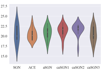
In Table 8, we see that each adaptive SGN model outperforms vanilla SGN on all the datasets. Based on the 12 running results, the violin plots are given in Figure 3. Basically, most differences in Table 8 are significant except for SIM on which no difference is significant ($p$-value $>0.05$).

(a) WS

(b) SIM

(c) REL

(d) MTurk287

(e) MTurk771

(f) RW

(g) MEN

(h) MC

(i) RG

(j) SimLex

Figure 3: Violin Plots of the Word Similarity Task.

(a) Semantic

(b) Syntactic

(c) Total Accuracy

Figure 4: Violin Plots of the Word Analogy Task.

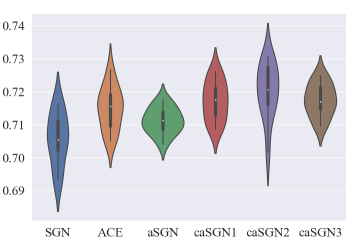
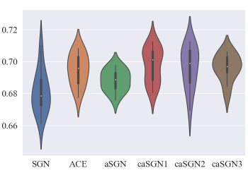
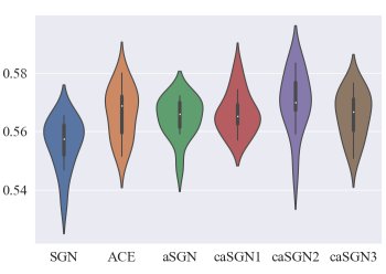
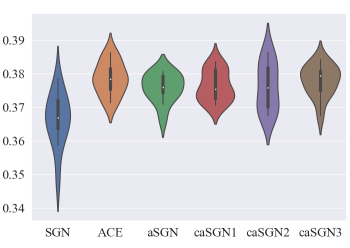
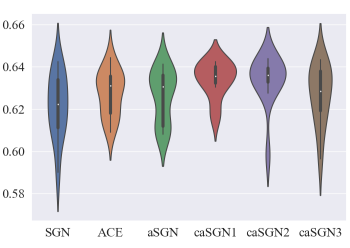
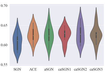
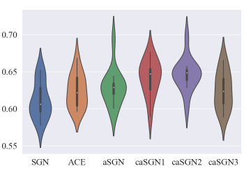
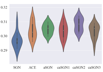
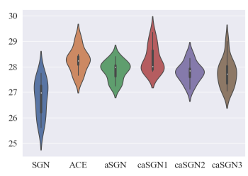
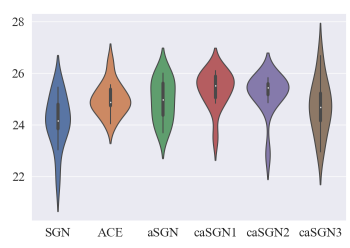
In Table 9, adaptive WCC models (especially conditional adaptive models) still outperform others. More precisely, there is no statistical significance difference on Semantic but the differences for total accuracy are significant except for caSGN3. the The violin plots are given in Figure 4.

Models	WS	SIM	REL	MT287	MT771	RW	MEN	MC	RG	SimLex
SGN	68.07	71.90	65.40	63.77	54.36	35.53	60.64	54.62	56.03	26.79
ACE	69.03	72.24	65.87	64.72	55.50	36.41	61.71	58.02	56.71	29.87
aSGN	68.66	71.80	65.80	65.27	54.44	35.55	60.74	52.17	54.68	26.90
caSGN1	68.83	71.67	65.36	64.32	53.76	36.85	60.11	57.34	54.89	28.15
caSGN2	70.10	73.23	67.10	65.72	55.07	36.75	61.04	57.60	57.93	28.73
caSGN3	69.63	73.07	66.80	64.79	54.19	36.25	60.70	59.21	58.42	26.96

Table 10: Spearman’s $\rho$ ($\ast 100$) of 50-dimension word embeddings on the word similarity tasks (text8).

Model	Semantic	Syntactic	Total
SGN	15.47	20.83	18.60
ACE	17.89	20.56	19.45
aSGN	16.83	21.46	19.53
caSGN1	17.99	20.09	19.22
caSGN2	17.53	21.15	19.64
caSGN3	17.91	20.79	19.59

Table 11: Accuracy of 50-dimension word embeddings on the word analogy task (text8).

B.2 Results of different word dimensions

We provide results of 50-dimension word embeddings in Table 10 and Table 11, and we also provide results of 200-dimension word embeddings in Table 12 and Table 13. We can see that experimental results verify that the observations are robust across different word dimensions.

Models	WS	SIM	REL	MT287	MT771	RW	MEN	MC	RG	SimLex
SGN	70.94	74.41	68.17	63.43	56.42	37.87	62.33	66.14	61.92	31.03
ACE	71.76	74.84	68.72	65.52	57.80	40.11	63.75	70.44	68.19	32.14
aSGN	71.96	74.95	69.50	64.61	58.19	39.02	63.73	66.03	64.80	32.66
caSGN1	69.16	71.72	67.99	62.52	57.50	38.48	65.61	70.26	66.98	31.37
caSGN2	72.23	74.80	69.67	65.09	58.01	38.63	64.75	68.43	68.02	32.86
caSGN3	71.44	72.46	71.28	65.33	57.54	39.84	66.42	64.85	69.14	32.88

Table 12: Spearman’s $\rho$ ($\ast 100$) of 200-dimension word embeddings on the word similarity tasks (text8).

Model	Semantic	Syntactic	Total
SGN	28.56	26.12	27.13
ACE	28.70	27.56	28.03
aSGN	27.10	27.94	27.59
caSGN1	27.63	28.47	28.12
caSGN2	31.59	27.23	29.05
caSGN3	32.67	28.15	29.02

Table 13: Accuracy of 200-dimension word embeddings on the word analogy task (text8).

Appendix C Further discussions

C.1 Limitation: time complexity

Arguably, one of the reasons for using NCE (Gutmann and Hyvärinen, 2012) is the efficiency gain in terms of time complexity. As each adaptive SGN becomes complex due to the training of the generator, it would likely require growing amount of time. In fact, compared with vanilla SGN, the running time of adaptive SGN models has increased more than tenfold.

However, word embeddings, or even other embeddings, are usually pre-trained for downstream tasks. Thus the computation is a one-off cost. Moreover, there are many specific tricks that can accelerate the training of GAN. In addition to the way mentioned in Section 4.6.2, one can see Bose, Ling, and Cao (2018) and Budhkar et al. (2019) for more suggestions.

C.2 WCC vs NCE

NLP researchers tend to regard SGN as an application of NCE to word embedding. We however assert that this understanding is incorrect. Agreeably both SGN and NCE uses noise samples to construct a binary classification problem, and it is possible to convert NCE to a conditional version so that resulting binary classification problem looks the same as that in SGN. However, NCE and SGN differ significantly.

NCE aims at learning a possibly unnormalized “density function” $f$ on a space of examples, through a set of observed examples; the starting point of NCE is setting up the function $f$. NCE then draws noise examples to form a negative class and reformulates the learning problem as a binary classification problem. It is remarkable that the parametrization of $f$ is independent of any noise distribution used in NCE.

SGN aims at learning the representation of the elements in a space (where each element is a word-context pair); the starting point of SGN is a binary classification formulation. That is, in SGN, there does not exist a parametrized density function independent of the choice of noise distribution. If one must equate SGN with a special case of NCE, then the effective density model in SGN would have to be parametrized by the noise distribution.

This difference between NCE and SGN also result in their differences in training: in NCE, one must be able to evaluate the noise distribution, but this is not required in SGN; in NCE, the partition function of the unnormalized density function f must also be estimated during training, but this is also not required in SGN. Thus although SGN is inspired by NCE, it is not NCE.

The distinction of the two extends to distinguishing WCC from NCE. Specifically WCC is a generalization of SGN to allowing more general forms of noise distribution. This generalization is “orthogonal” to the difference between NCE and SGN. Although the formalism of NCE allows any noise distribution, negative sampling with arbitrary noise distribution is established for the first time in this paper. When generalizing SGN to WCC, the PMI-MF result no longer holds. Another contribution of this paper is establishing the “correctness” of WCC in Corollary 1.

C.3 WCC vs ACE

ACE may be viewed as an adaptive conditional member of WCC, with a structure corresponding to Figure 1 (a) or (b) in Section 3.4 with variable Z deleted.

C.4 WCC vs BERT

Although the success of language models like BERT boils down to the complex structures (e.g., Transformer) rather than negative sampling (NS), these complex structure based models are already contained in the WCC framework. More precisely, the functions $f$,$g$ and $s$ in Section 3.2 are only taken by the simplest choices , and they can be more complicated. For example, $s$ can be a learnable neural network instead of an inner product. Specifically, if the model of $f$ is taken as Transformer or LSTM, which is essential to compare to BERT or ELMo, WCC will convert to the pre-trained model from the pre-trained embedding. Since the analysis is structure-independent, the theoretical results still hold. In addition, the language model can be regarded as a special case of the Continuous Bag of Words (CBOW) model with modified definitions of "context" and "window", so it also has the NS version. Particularly, on the Masked LM task of BERT, one can replace the Softmax layer by NS scheme, and on the Next Sentence Prediction task, one can maximize the similarity of the sentence pairs and minimize the similarity of randomly sampled sentences. In these cases, our analysis will be helpful. We leave these studies to the researchers who have enough computation resources to run the pre-training process of BERT.

C.5 Performance gain of WCC over existing models

The main objective of this paper is to present a unifying principle for SGN-like models, not to develop a BERT-like “super model” for word embedding. Word embedding and more generally representation learning have witnessed great successes in recent years. However the fundamental principles underlying these models are poorly explored. For example, even the problem of “representation learning” is poorly defined: except relying some downstream tasks to evaluate a learned representation, very little has been developed pertaining to the metrics or principles for word-embedding alike representation learning; what makes a “good” representation remains elusive. In this respect, Corollary 1 of this paper and PMI-MF are among the only results, to the best of our knowledge.

Despite our theoretical focus, this paper does yield new models that outperform the existing models. Compared with 3/4-ugSGN, our models not only performs significantly better, they are also more “negative-sample efficient”: our adaptive samplers draw one noise sample per data sample, whereas 3/4-ugSGN draws 5 noise samples per data sample. The fact that ACE also performs well should not be taken negatively on our results. As stated earlier, ACE is essentially an adaptive conditional member of WCC. Its good performance further endorses some claims of our paper, namely that WCC is a useful generalization and that adaptive conditional schemes can be advantageous. Nonetheless, the new models discovered in this work still significantly outperform ACE on some tasks.

References

- Agirre et al. (2009) Agirre, E.; Alfonseca, E.; Hall, K.; Kravalova, J.; Paşca, M.; and Soroa, A. 2009. A study on similarity and relatedness using distributional and wordnet-based approaches. In Proceedings of Human Language Technologies: The 2009 Annual Conference of the North American Chapter of the Association for Computational Linguistics, 19–27.
- Bose, Ling, and Cao (2018) Bose, A. J.; Ling, H.; and Cao, Y. 2018. Adversarial contrastive estimation. In Proceedings of the 56th Annual Meeting of the Association for Computational Linguistics (Volume 1: Long Papers), 1021–1032.
- Brown et al. (2020) Brown, T. B.; Mann, B.; Ryder, N.; Subbiah, M.; Kaplan, J.; Dhariwal, P.; Neelakantan, A.; Shyam, P.; Sastry, G.; Askell, A.; et al. 2020. Language models are few-shot learners. arXiv preprint arXiv:2005.14165.
- Bruni et al. (2012) Bruni, E.; Boleda, G.; Baroni, M.; and Tran, N.-K. 2012. Distributional semantics in technicolor. In Proceedings of the 50th Annual Meeting of the Association for Computational Linguistics (Volume 1: Long Papers), 136–145.
- Budhkar et al. (2019) Budhkar, A.; Vishnubhotla, K.; Hossain, S.; and Rudzicz, F. 2019. Generative adversarial networks for text using word2vec intermediaries. In Proceedings of the 4th Workshop on Representation Learning for NLP, 15–26.
- Chen et al. (2018) Chen, L.; Yuan, F.; Jose, J. M.; and Zhang, W. 2018. Improving negative sampling for word representation using self-embedded features. In Proceedings of the Eleventh ACM International Conference on Web Search and Data Mining, 99–107.
- Dai et al. (2019) Dai, Q.; Li, Q.; Zhang, L.; and Wang, D. 2019. Ranking network embedding via adversarial learning. In Advances in Knowledge Discovery and Data Mining - 23rd Pacific-Asia Conference, 27–39.
- Devlin et al. (2019) Devlin, J.; Chang, M.-W.; Lee, K.; and Toutanova, K. 2019. Bert: Pre-training of deep bidirectional transformers for language understanding. In Proceedings of the 2019 Conference of the North American Chapter of the Association for Computational Linguistics: Human Language Technologies (Volume 1: Long and Short Papers), 4171–4186.
- Finkelstein et al. (2002) Finkelstein, L.; Gabrilovich, E.; Matias, Y.; Rivlin, E.; Solan, Z.; Wolfman, G.; and Ruppin, E. 2002. Placing search in context: The concept revisited. ACM Transactions on information systems 20(1):116–131.
- Goodfellow et al. (2014) Goodfellow, I.; Pouget-Abadie, J.; Mirza, M.; Xu, B.; Warde-Farley, D.; Ozair, S.; Courville, A.; and Bengio, Y. 2014. Generative adversarial nets. In Advances in neural information processing systems, 2672–2680.
- Guo et al. (2018) Guo, G.; Ouyang, S.; Yuan, F.; and Wang, X. 2018. Approximating word ranking and negative sampling for word embedding. In Proceedings of the Twenty-Seventh International Joint Conference on Artificial Intelligence, 4092–4098.
- Gutmann and Hyvärinen (2012) Gutmann, M., and Hyvärinen, A. 2012. Noise-contrastive estimation of unnormalized statistical models, with applications to natural image statistics. Journal of Machine Learning Research 13:307–361.
- Halawi et al. (2012) Halawi, G.; Dror, G.; Gabrilovich, E.; and Koren, Y. 2012. Large-scale learning of word relatedness with constraints. In Proceedings of the 18th ACM SIGKDD international conference on Knowledge discovery and data mining, 1406–1414.
- Hill, Reichart, and Korhonen (2015) Hill, F.; Reichart, R.; and Korhonen, A. 2015. Simlex-999: Evaluating semantic models with (genuine) similarity estimation. Computational Linguistics 41(4):665–695.
- Jang, Gu, and Poole (2017) Jang, E.; Gu, S.; and Poole, B. 2017. Categorical reparameterization with gumbel-softmax. In International Conference on Learning Representations.
- Jordan (1995) Jordan, M. I. 1995. Why the logistic function? a tutorial discussion on probabilities and neural networks.
- Kingma and Welling (2014) Kingma, D. P., and Welling, M. 2014. Auto-encoding variational bayes. In International Conference on Learning Representations.
- Labeau and Allauzen (2018) Labeau, M., and Allauzen, A. 2018. Learning with noise-contrastive estimation: Easing training by learning to scale. In Proceedings of the 27th International Conference on Computational Linguistics, 3090–3101.
- Levy and Goldberg (2014) Levy, O., and Goldberg, Y. 2014. Neural word embedding as implicit matrix factorization. In Advances in neural information processing systems, 2177–2185.
- Luong, Socher, and Manning (2013) Luong, T.; Socher, R.; and Manning, C. 2013. Better word representations with recursive neural networks for morphology. In Proceedings of the Seventeenth Conference on Computational Natural Language Learning, 104–113.
- Ma and Collins (2018) Ma, Z., and Collins, M. 2018. Noise contrastive estimation and negative sampling for conditional models: Consistency and statistical efficiency. In Proceedings of the 2018 Conference on Empirical Methods in Natural Language Processing, Brussels, Belgium, October 31 - November 4, 2018, 3698–3707.
- Ma and Hovy (2016) Ma, X., and Hovy, E. 2016. End-to-end sequence labeling via bi-directional lstm-cnns-crf. In Proceedings of the 54th Annual Meeting of the Association for Computational Linguistics (Volume 1: Long Papers), 1064–1074.
- Maddison, Mnih, and Teh (2017) Maddison, C. J.; Mnih, A.; and Teh, Y. W. 2017. The concrete distribution: A continuous relaxation of discrete random variables. In International Conference on Learning Representations.
- Mahoney (2011) Mahoney, M. 2011. Large text compression benchmark. URL: http://www. mattmahoney. net/text/text. html.
- Melamud, Dagan, and Goldberger (2017) Melamud, O.; Dagan, I.; and Goldberger, J. 2017. A simple language model based on PMI matrix approximations. In Proceedings of the 2017 Conference on Empirical Methods in Natural Language Processing, 1860–1865.
- Mikolov et al. (2013a) Mikolov, T.; Chen, K.; Corrado, G.; and Dean, J. 2013a. Efficient estimation of word representations in vector space. arXiv preprint arXiv:1301.3781.
- Mikolov et al. (2013b) Mikolov, T.; Sutskever, I.; Chen, K.; Corrado, G. S.; and Dean, J. 2013b. Distributed representations of words and phrases and their compositionality. In Advances in neural information processing systems, 3111–3119.
- Miller and Charles (1991) Miller, G. A., and Charles, W. G. 1991. Contextual correlates of semantic similarity. Language and cognitive processes 6(1):1–28.
- Mu, Yang, and Zheng (2019) Mu, C. M.; Yang, G.; and Zheng, Y. J. 2019. Revisiting skip-gram negative sampling model with rectification. In Intelligent Computing-Proceedings of the Computing Conference, 485–497.
- Pennington, Socher, and Manning (2014) Pennington, J.; Socher, R.; and Manning, C. 2014. Glove: Global vectors for word representation. In Proceedings of the 2014 Conference on Empirical Methods in Natural Language Processing, 1532–1543.
- Peters et al. (2018) Peters, M.; Neumann, M.; Iyyer, M.; Gardner, M.; Clark, C.; Lee, K.; and Zettlemoyer, L. 2018. Deep contextualized word representations. In Proceedings of the 2018 Conference of the North American Chapter of the Association for Computational Linguistics: Human Language Technologies (Volume 1: Long Papers), 2227–2237.
- Radinsky et al. (2011) Radinsky, K.; Agichtein, E.; Gabrilovich, E.; and Markovitch, S. 2011. A word at a time: computing word relatedness using temporal semantic analysis. In Proceedings of the 20th International Conference on World Wide Web, 337–346.
- Rezende, Mohamed, and Wierstra (2014) Rezende, D. J.; Mohamed, S.; and Wierstra, D. 2014. Stochastic backpropagation and approximate inference in deep generative models. In International Conference on Machine Learning, 1278–1286.
- Rubenstein and Goodenough (1965) Rubenstein, H., and Goodenough, J. B. 1965. Contextual correlates of synonymy. Commun. ACM 8(10):627–633.
- Sang and Meulder (2003) Sang, E. F. T. K., and Meulder, F. D. 2003. Introduction to the conll-2003 shared task: Language-independent named entity recognition. In Proceedings of the Seventh Conference on Natural Language Learning, 142–147.
- Soleimani and Matwin (2018) Soleimani, B. H., and Matwin, S. 2018. Spectral word embedding with negative sampling. In Proceedings of the Thirty-Second AAAI Conference on Artificial Intelligence, 5481–5487.
- Sun et al. (2016) Sun, F.; Guo, J.; Lan, Y.; Xu, J.; and Cheng, X. 2016. Sparse word embeddings using l 1 regularized online learning. In Proceedings of the Twenty-Fifth International Joint Conference on Artificial Intelligence, 2915–2921.
- Wang et al. (2017) Wang, J.; Yu, L.; Zhang, W.; Gong, Y.; Xu, Y.; Wang, B.; Zhang, P.; and Zhang, D. 2017. Irgan: A minimax game for unifying generative and discriminative information retrieval models. In Proceedings of the 40th International ACM SIGIR conference on Research and Development in Information Retrieval, 515–524.
- Wang, Li, and Pan (2018) Wang, P.; Li, S.; and Pan, R. 2018. Incorporating GAN for negative sampling in knowledge representation learning. In Proceedings of the Thirty-Second AAAI Conference on Artificial Intelligence, 2005–2012.
- Wang, Liu, and Zhao (2017) Wang, B.; Liu, K.; and Zhao, J. 2017. Conditional generative adversarial networks for commonsense machine comprehension. In Proceedings of the Twenty-Sixth International Joint Conference on Artificial Intelligence, 4123–4129.
- Williams (1992) Williams, R. J. 1992. Simple statistical gradient-following algorithms for connectionist reinforcement learning. Machine Learning 8:229–256.
- Yang et al. (2019) Yang, Z.; Dai, Z.; Yang, Y.; Carbonell, J.; Salakhutdinov, R. R.; and Le, Q. V. 2019. Xlnet: Generalized autoregressive pretraining for language understanding. In Advances in neural information processing systems, 5754–5764.
- Zhang and Zweigenbaum (2018) Zhang, Z., and Zweigenbaum, P. 2018. Gneg: graph-based negative sampling for word2vec. In Proceedings of the 56th Annual Meeting of the Association for Computational Linguistics (Volume 2: Short Papers), 566–571.