GraphNorm: A Principled Approach to Accelerating
Graph Neural Network Training
Abstract
Normalization is known to help the optimization of deep neural networks. Curiously, different architectures require specialized normalization methods. In this paper, we study what normalization is effective for Graph Neural Networks (GNNs). First, we adapt and evaluate the existing methods from other domains to GNNs. Faster convergence is achieved with InstanceNorm compared to BatchNorm and LayerNorm. We provide an explanation by showing that InstanceNorm serves as a preconditioner for GNNs, but such preconditioning effect is weaker with BatchNorm due to the heavy batch noise in graph datasets. Second, we show that the shift operation in InstanceNorm results in an expressiveness degradation of GNNs for highly regular graphs. We address this issue by proposing GraphNorm with a learnable shift. Empirically, GNNs with GraphNorm converge faster compared to GNNs using other normalization. GraphNorm also improves the generalization of GNNs, achieving better performance on graph classification benchmarks.
1 Introduction
Recently, there has been a surge of interest in Graph Neural Networks (GNNs) for learning with graphs (Gori et al., 2005; Scarselli et al., 2008; Hamilton et al., 2017; Kipf & Welling, 2017; Velickovic et al., 2018; Xu et al., 2018; Ying et al., 2021). GNNs learn node and graph representations by recursively aggregating and updating the node representations from neighbor representations (Gilmer et al., 2017). Empirically, GNNs have succeeded in a variety of tasks such as computational chemistry (Stokes et al., 2020), recommendation systems (Ying et al., 2018), and visual question answering (Santoro et al., 2017). Theoretically, existing works have studied GNNs through the lens of expressive power (Keriven & Peyré, 2019; Xu et al., 2019; Sato et al., 2019; Loukas, 2020; Ying et al., 2021), generalization (Scarselli et al., 2018; Du et al., 2019b; Xu et al., 2020), and extrapolation (Xu et al., 2021). However, the optimization of GNNs is less well understood, and in practice, the training of GNNs is often unstable and the convergence is slow (Xu et al., 2019).
In this paper, we study how to improve the training of GNNs via normalization. Normalization methods shift and scale the hidden representations and are shown to help the optimization for deep neural networks (Ioffe & Szegedy, 2015; Ulyanov et al., 2016; Ba et al., 2016; Salimans & Kingma, 2016; Xiong et al., 2020; Salimans et al., 2016; Miyato et al., 2018; Wu & He, 2018; Santurkar et al., 2018). Curiously, no single normalization helps in every domain, and different architectures require specialized methods. For example, Batch normalization (BatchNorm) is a standard component in computer vision (Ioffe & Szegedy, 2015); Layer normalization (LayerNorm) is popular in natural language processing (Ba et al., 2016; Xiong et al., 2020); Instance normalization (InstanceNorm) has been found effective for style transfer tasks (Ulyanov et al., 2016) . This motivates the question: What normalization methods are effective for GNNs?
We take an initial step towards answering the question above. First, we adapt the existing methods from other domains, including BatchNorm, LayerNorm, and InstanceNorm, to GNNs and evaluate their performance with extensive experiments on graph classification tasks. We observe that our adaptation of InstanceNorm to GNNs, which for each individual graph normalizes its node hidden representations, obtains much faster convergence compared to BatchNorm and LayerNorm. We provide an explanation for the success of InstanceNorm by showing that the shift operation in InstanceNorm serves as a preconditioner of the graph aggregation operation. Empirically, such preconditioning makes the optimization curvature smoother and makes the training more efficient. We also explain why the widely used BatchNorm does not bring the same level of acceleration. The variance of the batch-level statistics on graph datasets is much larger if we apply the normalization across graphs in a batch instead of across individual graphs. The noisy statistics during training may lead to unstable optimization.
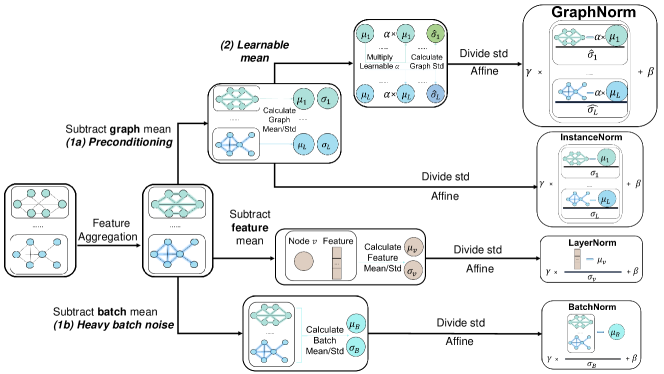
Second, we show that the adaptation of InstanceNorm to GNNs, while being helpful in general, has limitations. The shift operation in InstanceNorm, which subtracts the mean statistics from node hidden representations, may lead to an expressiveness degradation for GNNs. Specifically, for highly regular graphs, the mean statistics contain graph structural information, and thus removing them could hurt the performance. Based on our analysis, we propose GraphNorm to address the issue of InstanceNorm with a learnable shift (Step 2 in Figure 1). The learnable shift could learn to control the ideal amount of information to preserve for mean statistics. Together, GraphNorm normalizes the hidden representations across nodes in each individual graph with a learnable shift to avoid the expressiveness degradation while inheriting the acceleration effect of the shift operation.
We validate the effectiveness of GraphNorm on eight popular graph classification benchmarks. Empirical results confirm that GraphNorm consistently improves the speed of converge and stability of training for GNNs compared to those with BatchNorm, InstanceNorm, LayerNorm, and those without normalization. Furthermore, GraphNorm helps GNNs achieve better generalization performance on most benchmarks.
1.1 Related Work
Closely related to our work, InstanceNorm (Ulyanov et al., 2016) is originally proposed for real-time image generation. Variants of InstanceNorm are also studied in permutation equivalent data processing (Yi et al., 2018; Sun et al., 2020). We instead adapt InstanceNorm to GNNs and find it helpful for the training of GNNs. Our proposed GraphNorm builds on and improves InstanceNorm by addressing its expressiveness degradation with a learnable shift.
Few works have studied normalization in the GNN literature. Xu et al. (2019) adapts BatchNorm to GIN as a plug-in component. A preliminary version of Dwivedi et al. (2020) normalizes the node features with respect to the graph size. Our GraphNorm is size-agnostic and significantly differs from the graph size normalization. More discussions on other normalization methods are in Appendix E.
The reason behind the effectiveness of normalization has been intensively studied. While scale and shift are the main components of normalization, most existing works focus on the scale operation and the “scale-invariant” property: With a normalization layer after a linear (or convolutional) layer, the output values remain the same as the weights are scaled. Hence, normalization decouples the optimization of direction and length of the parameters (Kohler et al., 2019), implicitly tunes the learning rate (Ioffe & Szegedy, 2015; Hoffer et al., 2018; Arora et al., 2018b; Li & Arora, 2019), and smooths the optimization landscape (Santurkar et al., 2018). Our work offers a different view by instead showing specific shift operation has the preconditioning effect and can accelerate the training of GNNs.
2 Preliminaries
We begin by introducing our notations and the basics of GNNs. Let denote a graph where , is the number of nodes. Let the feature vector of node be . We denote the adjacency matrix of a graph as with if and otherwise. The degree matrix associated with is defined as where .
Graph Neural Networks. GNNs use the graph structure and node features to learn the representations of nodes and graphs. Modern GNNs follow a neighborhood aggregation strategy (Sukhbaatar et al., 2016; Kipf & Welling, 2017; Hamilton et al., 2017; Velickovic et al., 2018; Monti et al., 2017; Ying et al., 2021), where the representation of a node is iteratively updated by aggregating the representation of its neighbors. To be concrete, we denote as the representation of at the -th layer and define . We use AGGREGATE to denote the aggregation function in the -th layer:
| (1) |
where is the set of nodes adjacent to . Different GNNs can be obtained by choosing different AGGREGATE functions. Graph Convolutional Networks (GCN) (Kipf & Welling, 2017) can be defined in matrix form as:
| (2) |
where ReLU stands for rectified linear unit, is the feature matrix at the -th layer where denotes the feature dimension, and is the parameter matrix in layer . , where and is the degree matrix of . is the identity matrix.
Graph Isomorphism Network (GIN) (Xu et al., 2019) is defined in matrix form as
| (3) |
where MLP stands for multilayer perceptron, is a learnable parameter and .
For a -layer GNN, the outputs of the final layer, i.e., ,, will be used for prediction. For graph classification tasks, we can apply a READOUT function, e.g., summation, to aggregate node features to obtain the entire graph’s representation . A classifier can be applied upon to predict the labels.
Normalization. Generally, given a set of values , a normalization operation first shifts each by the mean , and then scales them down by standard deviation : , where and are learnable parameters, and . The major difference among different existing normalization methods is which set of feature values the normalization is applied to. For example, in computer vision, BatchNorm normalizes the feature values in the same channel across different samples in a batch. In NLP, LayerNorm normalizes the feature values at each position in a sequence separately.
3 Evaluating and Understanding Normalization for GNNs
In this section, we first adapt and evaluate existing normalization methods to GNNs. Then we give an explanation of the effectiveness of the variant of InstanceNorm, and show why the widely used BatchNorm fails to have such effectiveness. The understanding inspires us to develop better normalization methods, e.g., GraphNorm.
3.1 Adapting and Evaluating Normalization for GNNs
To investigate what normalization methods are effective for GNNs, we first adapt three typical normalization methods, i.e., BatchNorm, LayerNorm, and InstanceNorm, developed in other domain to GNNs. We apply the normalization after the linear transformation as in previous works (Ioffe & Szegedy, 2015; Xiong et al., 2020; Xu et al., 2019). The general GNN structure equipped with a normalization layer can be represented as:
| (4) |
where is a function that applies to each node separately, is an matrix representing the neighbor aggregation, and is the weight/parameter matrix in layer . We can instantiate Eq. (4) as GCN and GIN, by setting proper and matrix . For example, if we set to be and set to be (Eq. (2)), then Eq. (4) becomes GCN with normalization; Similarly, by setting to be and to be (Eq. (3)), we recover GIN with normalization.
We then describe the concrete operations of the adaptations of the normalization methods. Consider a batch of graphs where is the batch size. Let be the number of nodes in graph . We generally denote as the inputs to the normalization module, e.g., the -th feature value of node of graph , . The adaptations take the general form:
| (5) |
where the scopes of mean , standard deviation , and affine parameters differ for different normalization methods. For BatchNorm, normalization and the computation of and are applied to all values in the same feature dimension across the nodes of all graphs in the batch as in Xu et al. (2019), i.e., over dimensions of . To adapt LayerNorm to GNNs, we view each node as a basic component, resembling words in a sentence, and apply normalization to all feature values across different dimensions of each node, i.e., over dimension of . For InstanceNorm, we regard each graph as an instance. The normalization is then applied to the feature values across all nodes for each individual graph, i.e., over dimension of .
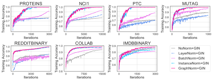
In Figure 2 we show training curves of different normalization methods in graph classification tasks. We find that LayerNorm hardly improves the training process in most tasks, while our adaptation of InstanceNorm can largely boost the training speed compared to other normalization methods. The test performances have similar trends. We summarize the final test accuracies in Table 1. In the following subsections, we provide an explanation for the success of InstanceNorm and its benefits compared to BatchNorm, which is currently adapted in many GNNs.
3.2 Shift in InstanceNorm as a Preconditioner
As mentioned in Section 1.1, the scale-invariant property of the normalization has been investigated and considered as one of the ingredients that make the optimization efficient. In our analysis of normalizations for GNNs, we instead take a closer look at the shift operation in the normalization. Compared to the image and sequential data, the graph is explicitly structured, and the neural networks exploit the structural information directly in the aggregation of the neighbors, see Eq. (1). Such uniqueness of GNNs makes it possible to study how the shift operation interplays with the graph data in detail.
We show that the shift operation in our adaptation of InstanceNorm serves as a preconditioner of the aggregation in GNNs and hypothesize this preconditioning effect can boost the training of GNNs. Though the current theory of deep learning has not been able to prove and compare the convergence rate in the real settings, we calculate the convergence rate of GNNs on a simple but fully characterizable setting to give insights on the benefit of the shift operation.
fWe first formulate our adaptation of InstanceNorm in the matrix form. Mathematically, for a graph of nodes, denote . is the matrix form of the shift operation, i.e., for any vector , . Then the normalization together with the aggregation can be represented as111Standard normalization has an additional affine operation after shifting and scaling. Here we omit it in Eq. 6 for better demonstration. Adding this operation will not affect the theoretical analysis.
| (6) |
where is the scaling, and is the GNN aggregation matrix. Each is the standard deviation of the values of the -th features among the nodes in the graph we consider. We can see that, in the matrix form, shifting feature values on a single graph is equivalent to multiplying as in Eq. (6). Therefore, we further check how this operation affects optimization. In particular, we examine the singular value distribution of . The following theorem shows that has a smoother singular value distribution than , i.e., serves as a preconditioner of .
Theorem 3.1 (Shift Serves as a Preconditioner of ).
Let be defined as in Eq. (6), be the singular values of . We have is one of the singular values of , and let other singular values of be . Then we have
| (7) |
where or only if there exists one of the right singular vectors of associated with satisfying .
The proof can be found in Appendix A.1.
We hypothesize that precoditioning can help the optimization. In the case of optimizing the weight matrix , we can see from Eq. (6) that after applying normalization, the term in the gradient of will become which makes the optimization curvature of smoother, see Appendix A.5 for more discussions. Similar preconditioning effects are believed to improve the training of deep learning models (Duchi et al., 2011; Kingma & Ba, 2015), and classic wisdom in optimization has also shown that preconditioning can accelerate the convergence of iterative methods (Axelsson, 1985; Demmel, 1997). Unfortunately, current theoretical toolbox only has a limited power on the optimization of deep learning models. Global convergence rates have only been proved for either simple models, e.g., linear models (Arora et al., 2018a), or extremely overparameterized models (Du et al., 2018; Allen-Zhu et al., 2019; Du et al., 2019a; Cai et al., 2019; Du et al., 2019b; Zou et al., 2020). To support our hypothesis that preconditioning may suggest better training, we investigate a simple but characterizable setting of training a linear GNN using gradient descent in Appendix A.2. In this setting, we prove that:
Proposition 3.1 (Concrete Example Showing Shift can Accelerate Training (Informal)).
With high probability over randomness of data generation, the parameter of the model with shift at step converges to the optimal parameter linearly:
where is the convergence rate.
Similarly, the parameter of the vanilla model converges linearly, but with a slower rate:
which indicates that the model with shift converges faster than the vanilla model.
The proof can be found in Appendix A.2.

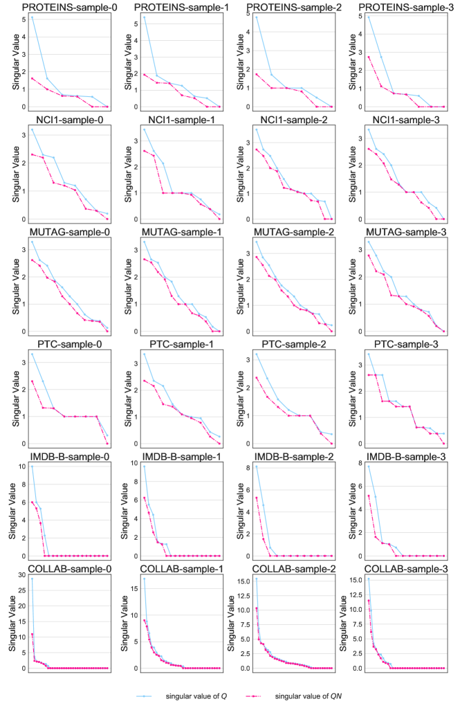
To check how much the matrix improves the distribution of the spectrum of matrix in real practice, we sample graphs from different datasets for illustration, as showed in Figure 3 (more visualizations for different types of graph can be found in Appendix D.1). We can see that the singular value distribution of is much smoother, and the condition number is improved. Note that for a multi-layer GNN, the normalization will be applied in each layer. Therefore, the overall improvement of such preconditioning can be more significant.
3.3 Heavy Batch Noise in Graphs Makes BatchNorm Less Effective
The above analysis shows the adaptation of InstanceNorm has the effect of preconditioning the aggregation of GNNs. Then a natural question is whether a batch-level normalization for GNNs (Xu et al., 2019) has similar advantages. We show that BatchNorm is less effective in GNNs due to heavy batch noise on graph data.
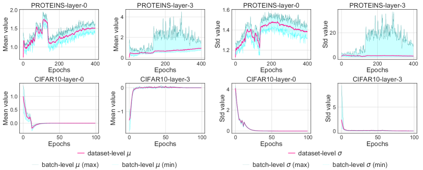
In BatchNorm, the mean and standard deviation are calculated in a sampled batch during training, which can be viewed as random variables by the randomness of sampling. During testing, the estimated dataset-level statistics (running mean and standard deviation ) are used instead of the batch-level statistics (Ioffe & Szegedy, 2015). To apply Theorem 3.1 to BatchNorm for the preconditioning effect, one could potentially view all graphs in a dataset as subgraphs in a super graph. Hence, Theorem 3.1 applies to BatchNorm if the batch-level statistics are well-concentrated around dataset-level statistics, i.e., and . However, the concentration of batch-level statistics is heavily domain-specific. While Shen et al. (2020) find the variation of batch-level statistics in typical networks is small for computer vision, the concentration of batch-level statistics is still unknown for GNNs.
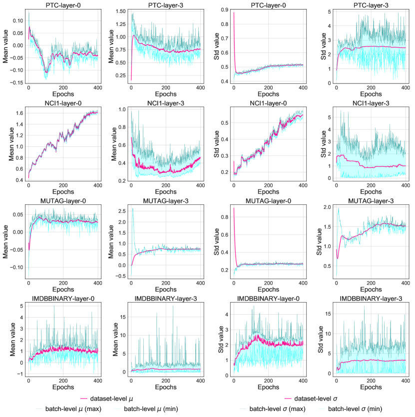
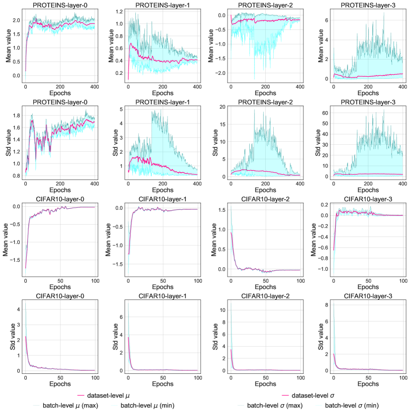
We study how the batch-level statistics deviate from the dataset-level statistics . For comparison, we train a 5-layer GIN with BatchNorm on the PROTEINS dataset and train a ResNet18 (He et al., 2016) on the CIFAR10 dataset. We set batch size to 128. For each epoch, we record the batch-level max/min mean and standard deviation for the first and the last BatchNorm layer on a randomly selected dimension across batches. In Figure 4, pink line denotes the dataset-level statistics, and green/blue line denotes the max/min value of the batch-level statistics. We observe that for image tasks, the maximal deviation of the batch-level statistics from the dataset-level statistics is negligible (Figure 4) after a few epochs. In contrast, for the graph tasks, the variation of batch-level statistics stays large during training. Intuitively, the graph structure can be quite diverse and the a single batch cannot well represent the entire dataset. Hence, the preconditioning property also may not hold for BatchNorm. In fact, the heavy batch noise may bring instabilities to the training. More results may be found in Appendix D.2.
4 Graph Normalization
Although we provide evidence on the indispensability and advantages of our adaptation of InstanceNorm, simply normalizing the values in each feature dimension within a graph does not consistently lead to improvement. We show that in some situations, e.g., for regular graphs, the standard shift (e.g., shifting by subtracting the mean) may cause information loss on graph structures.
We consider -regular graphs, i.e., each node has a degree . We first look into the case that there are no available node features, then is set to be the one-hot encoding of the node degree (Xu et al., 2019). In a -regular graph, all nodes have the same encoding, and thus the columns of are the same. We study the output of the standard shift operation in the first layer, i.e., in Eq. (6). From the following proposition, we can see that when the standard shift operation is applied to GIN for a -regular graph described above, the information of degree is lost:
Proposition 4.1.
For a -regular graph with one-hot encodings as its features described above, we have for GIN, , i.e., the output of normalization layer is a zero matrix without any information of the graph structure.
Such information loss not only happens when there are no node features. For complete graphs, we can further show that even each node has different features, the graph structural information, i.e., adjacency matrix , will always be ignored after the standard shift operation in GIN:
Proposition 4.2.
For a complete graph (), we have for GIN, , i.e., graph structural information in will be removed after multiplying .
The proof of these two propositions can be found in Appendix A. Similar results can be easily derived for other architectures like GCN by substituting with . As we can see from the above analysis, in graph data, the mean statistics after the aggregation sometimes contain structural information. Discarding the mean will degrade the expressiveness of the neural networks. Note that the problem may not happen in image domain. The mean statistics of image data contains global information such as brightness. Removing such information in images will not change the semantics of the objects and thus will not hurt the classification performance.
This analysis inspires us to modify the current normalization method with a learnable parameter to automatically control how much the mean to preserve in the shift operation. Combined with the graph-wise normalization, we name our new method Graph Normalization, i.e., GraphNorm. For each graph , we generally denote value as the inputs to GraphNorm, e.g., the -th feature value of node , , . GraphNorm takes the following form:
| (8) |
where , and are the affine parameters as in other normalization methods. By introducing the learnable parameter for each feature dimension , we are able to learn how much the information we need to keep in the mean. It is easy to see that GraphNorm has stronger expressive power than InstanceNorm. Formally, we have the following fact:
Fact 1 (GraphNorm is strictly more expressive than InstanceNorm).
If , then there does not exist such that for any that the normalization is applied to, for any , where .
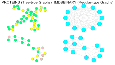
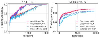
To validate our theory and the proposed GraphNorm in real-world data, we conduct an ablation study on two typical datasets, PROTEINS and IMDB-BINARY. As shown in Figure 5, the graphs from PROTEINS and IMDB-BINARY exhibit irregular-type and regular-type graphs, respectively. We train GIN/GCN using our adaptation of InstanceNorm and GraphNorm under the same setting in Section 5. The training curves are presented in Figure 5. The curves show that using a learnable slightly improves the convergence on PROTEINS, while significantly boost the training on IMDB-BINARY. This observation verify that shifting the feature values by subtracting the mean may lose information, especially for regular graphs. And the introduction of learnable shift in GraphNorm can effectively mitigate the expressive degradation.
| Datasets | MUTAG | PTC | PROTEINS | NCI1 | IMDB-B | RDT-B | COLLAB | |
|---|---|---|---|---|---|---|---|---|
| # graphs | 188 | 344 | 1113 | 4110 | 1000 | 2000 | 5000 | |
| # classes | 2 | 2 | 2 | 2 | 2 | 2 | 2 | |
| Avg # nodes | 17.9 | 25.5 | 39.1 | 29.8 | 19.8 | 429.6 | 74.5 | |
| WL subtree (Shervashidze et al., 2011) | 90.4 5.7 | 59.9 4.3 | 75.0 3.1 | 86.0 1.8 | 73.8 3.9 | 81.0 3.1 | 78.9 1.9 | |
| DCNN (Atwood & Towsley, 2016) | 67.0 | 56.6 | 61.3 | 62.6 | 49.1 | - | 52.1 | |
| DGCNN (Zhang et al., 2018) | 85.8 | 58.6 | 75.5 | 74.4 | 70.0 | - | 73.7 | |
| AWL (Ivanov & Burnaev, 2018) | 87.9 9.8 | - | - | - | 74.5 5.9 | 87.9 2.5 | 73.9 1.9 | |
| GIN+LayerNorm | 82.4 6.4 | 62.8 9.3 | 76.2 3.0 | 78.3 1,7 | 74.5 4,4 | 82.8 7.7 | 80.1 0.8 | |
| GIN+BatchNorm ((Xu et al., 2019)) | 89.4 5.6 | 64.6 7.0 | 76.2 2.8 | 82.7 1.7 | 75.1 5.1 | 92.4 2.5 | 80.2 1.9 | |
| GIN+InstanceNorm | 90.5 7.8 | 64.7 5.9 | 76.5 3.9 | 81.2 1.8 | 74.8 5.0 | 93.2 1.7 | 80.0 2.1 | |
| GIN+GraphNorm | 91.6 6.5 | 64.9 7.5 | 77.4 4.9 | 81.4 2.4 | 76.0 3.7 | 93.5 2.1 | 80.2 1.0 |
| Datasets | Ogbg-molhiv |
|---|---|
| # graphs | 41,127 |
| # classes | 2 |
| Avg # nodes | 25.5 |
| GCN (Hu et al., 2020) | 76.06 0.97 |
| GIN (Hu et al., 2020) | 75.58 1.40 |
| GCN+LayerNorm | 75.04 0.48 |
| GCN+BatchNorm | 76.22 0.95 |
| GCN+InstanceNorm | 78.18 0.42 |
| GCN+GraphNorm | 78.30 0.69 |
| GIN+LayerNorm | 74.79 0.92 |
| GIN+BatchNorm | 76.61 0.97 |
| GIN+InstanceNorm | 77.54 1.27 |
| GIN+GraphNorm | 77.73 1.29 |
5 Experiments
In this section, we evaluate and compare both the training and test performance of GraphNorm with other normalization methods on graph classification benchmarks.
Settings.
We use eight popularly used benchmark datasets of different scales in the experiments (Yanardag & Vishwanathan, 2015; Xu et al., 2019), including four medium-scale bioinformatics datasets (MUTAG, PTC, PROTEINS, NCI1), three medium-scale social network datasets (IMDB-BINARY, COLLAB, REDDIT-BINARY), and one large-scale bioinformatics dataset ogbg-molhiv, which is recently released on Open Graph Benchmark (OGB) (Hu et al., 2020). Dataset statistics are summarized in Table 1. We use two typical graph neural networks GIN (Xu et al., 2019) and GCN (Kipf & Welling, 2017) for our evaluations. Specifically, we use a five-layer GCN/GIN. For GIN, the number of sub-layers in MLP is set to 2. Normalization is applied to each layer. To aggregate global features on top of the network, we use SUM readout for MUTAG, PTC, PROTEINS and NCI1 datasets, and use MEAN readout for other datasets, as in Xu et al. (2019). Details of the experimental settings are presented in Appendix C.
Results.
We plot the training curves of GIN with GraphNorm and other normalization methods222The graph size normalization in the preliminary version of Dwivedi et al. (2020) does not show significant improvement on the training and test performance, so we do not report it. on different tasks in Figure 2. The results on GCN show similar trends, and are provided in Appendix D.3. As shown in Figure 2, GraphNorm enjoys the fastest convergence on all tasks. Compared to BatchNorm used in Xu et al. (2019), GraphNorm converges in roughly 5000/500 iterations on NCI1 and PTC datasets, while the model using BatchNorm does not even converge in 10000/1000 iterations. Remarkably, though InstanceNorm does not outperform other normalization methods on IMDB-BINARY, GraphNorm with learnable shift significantly boosts the training upon InstanceNorm and achieves the fastest convergence. We also validate the test performance and report the test accuracy in Table 1,2. The results show that GraphNorm also improves the generalization on most benchmarks.
For reference, we explain the possible reasons of higher test accuracy in two folds. First, as shown in Figure 2, using proper normalization helps the model find a minimum with a higher training accuracy. Second, as suggested by Hardt et al. (2016), faster training leads to smaller generalization gap. Since the test accuracy equals the training accuracy plus the generalization, these two views together suggest better normalization leads to better test performance.
5.1 Ablation Study
In this subsection, we summarize the results of some ablation studies, including BatchNorm with learnable shift, BatchNorm with running statistics and the effect of batch size. Due to the space limitation, the detailed results can be found in Appendix D.
BatchNorm with learnable shift.
We conduct experiments on BatchNorm to investigate whether simply introducing a learnable shift can already improve the existing normalization methods without concrete motivation of overcoming expressiveness degradation. Specifically, we equip BatchNorm with a similar learnable shift as GraphNorm and evaluate its performance. We find that the learnable shift cannot further improve upon BatchNorm (See Appendix D), which suggests the introduction of learnable shift in GraphNorm is critical.
BatchNorm with running statistics.
We study the variant of BatchNorm which uses running statistics to replace the batch-level mean and standard deviation (Similar idea is also proposed in Yan et al. (2019)). At first glance, this method may seem to be able to mitigate the problem of large batch noise. However, the running statistics change a lot during training, and using running statistics disables the model to back-propagate the gradients through mean and standard deviation. Results in Appendix D show this variant has even worse performance than BatchNorm.
The effect of batch size.
We further compare the GraphNorm with BatchNorm with different batch sizes (8, 16, 32, 64). As shown in Appendix D, our GraphNorm consistently outperforms the BatchNorm on all the settings.
6 Conclusion and Future Work
In this paper, we adapt and evaluate three well-used normalization methods, i.e., BatchNorm, LayerNorm, and InstanceNorm to GNNs. We give explanations for the successes and failures of these adaptations. Based on our understanding of the strengths and limitations of existing adaptations, we propose Graph Normalization, that builds upon the adaptation of InstanceNorm with a learnable shift to overcome the expressive degradation of the original InstanceNorm. Experimental results show GNNs with GraphNorm not only converge faster, but also achieve better generalization performance on several benchmark datasets.
Though seeking theoretical understanding of normalization methods in deep learning is challenging (Arora et al., 2018b) due to limited understanding on the optimization of deep learning models and characterization of real world data, we take an initial step towards finding effective normalization methods for GNNs with theoretical guidance in this paper. The proposed theories and hypotheses are motivated by several simple models. And we are not able to give concrete theoretical results to problems such as: the convergence rate of general GNNs with normalization, the spectrum of normalized by learnable shift, etc. We believe the analyses of more realistic but complicated settings, e.g., the dynamics of GraphNorm on deep GNNs, are good future directions.
Acknowledgements
We thank Mozhi Zhang and Ruosong Wang for helpful suggestions on the paper; Zhiyuan Li and Kaifeng Lyu for helpful discussion on the literature of normalization methods; and Prof. Yang Yuan for support of computational resources. This work was supported by National Key R&D Program of China (2018YFB1402600), Key-Area Research and Development Program of Guangdong Province (No. 2019B121204008), BJNSF (L172037), Beijing Academy of Artificial Intelligence, Project 2020BD006 supported by PKU-Baidu Fund, NSF CAREER award (1553284) and NSF III (1900933).
References
- Allen-Zhu et al. (2019) Allen-Zhu, Z., Li, Y., and Song, Z. A convergence theory for deep learning via over-parameterization. In International Conference on Machine Learning, pp. 242–252. PMLR, 2019.
- Arora et al. (2018a) Arora, S., Cohen, N., Golowich, N., and Hu, W. A convergence analysis of gradient descent for deep linear neural networks. In International Conference on Learning Representations, 2018a.
- Arora et al. (2018b) Arora, S., Li, Z., and Lyu, K. Theoretical analysis of auto rate-tuning by batch normalization. arXiv preprint arXiv:1812.03981, 2018b.
- Atwood & Towsley (2016) Atwood, J. and Towsley, D. Diffusion-convolutional neural networks. In Advances in neural information processing systems, pp. 1993–2001, 2016.
- Axelsson (1985) Axelsson, O. A survey of preconditioned iterative methods for linear systems of algebraic equations. BIT Numerical Mathematics, 25(1):165–187, 1985.
- Ba et al. (2016) Ba, J. L., Kiros, J. R., and Hinton, G. E. Layer normalization. arXiv preprint arXiv:1607.06450, 2016.
- Bruna et al. (2013) Bruna, J., Zaremba, W., Szlam, A., and LeCun, Y. Spectral networks and locally connected networks on graphs. arXiv preprint arXiv:1312.6203, 2013.
- Cai et al. (2019) Cai, T., Gao, R., Hou, J., Chen, S., Wang, D., He, D., Zhang, Z., and Wang, L. A gram-gauss-newton method learning overparameterized deep neural networks for regression problems. arXiv preprint arXiv:1905.11675, 2019.
- Chen et al. (2020) Chen, Y., Tang, X., Qi, X., Li, C.-G., and Xiao, R. Learning graph normalization for graph neural networks, 2020.
- Defferrard et al. (2016) Defferrard, M., Bresson, X., and Vandergheynst, P. Convolutional neural networks on graphs with fast localized spectral filtering. In Advances in neural information processing systems, pp. 3844–3852, 2016.
- Demmel (1997) Demmel, J. W. Applied numerical linear algebra, volume 56. Siam, 1997.
- Du et al. (2019a) Du, S., Lee, J., Li, H., Wang, L., and Zhai, X. Gradient descent finds global minima of deep neural networks. In International Conference on Machine Learning, pp. 1675–1685. PMLR, 2019a.
- Du et al. (2018) Du, S. S., Zhai, X., Poczos, B., and Singh, A. Gradient descent provably optimizes over-parameterized neural networks. In International Conference on Learning Representations, 2018.
- Du et al. (2019b) Du, S. S., Hou, K., Salakhutdinov, R. R., Poczos, B., Wang, R., and Xu, K. Graph neural tangent kernel: Fusing graph neural networks with graph kernels. In Advances in Neural Information Processing Systems, pp. 5724–5734, 2019b.
- Duchi et al. (2011) Duchi, J., Hazan, E., and Singer, Y. Adaptive subgradient methods for online learning and stochastic optimization. Journal of machine learning research, 12(Jul):2121–2159, 2011.
- Dwivedi et al. (2020) Dwivedi, V. P., Joshi, C. K., Laurent, T., Bengio, Y., and Bresson, X. Benchmarking graph neural networks. arXiv preprint arXiv:2003.00982, 2020.
- Gilmer et al. (2017) Gilmer, J., Schoenholz, S. S., Riley, P. F., Vinyals, O., and Dahl, G. E. Neural message passing for quantum chemistry. In International Conference on Machine Learning, pp. 1273–1272, 2017.
- Gori et al. (2005) Gori, M., Monfardini, G., and Scarselli, F. A new model for learning in graph domains. In Proceedings. 2005 IEEE International Joint Conference on Neural Networks, 2005., volume 2, pp. 729–734. IEEE, 2005.
- Hamilton et al. (2017) Hamilton, W., Ying, Z., and Leskovec, J. Inductive representation learning on large graphs. In Advances in neural information processing systems, pp. 1024–1034, 2017.
- Hardt et al. (2016) Hardt, M., Recht, B., and Singer, Y. Train faster, generalize better: Stability of stochastic gradient descent. In International Conference on Machine Learning, pp. 1225–1234. PMLR, 2016.
- He et al. (2016) He, K., Zhang, X., Ren, S., and Sun, J. Deep residual learning for image recognition. In Proceedings of the IEEE conference on computer vision and pattern recognition, pp. 770–778, 2016.
- Hoffer et al. (2018) Hoffer, E., Banner, R., Golan, I., and Soudry, D. Norm matters: efficient and accurate normalization schemes in deep networks. In Advances in Neural Information Processing Systems, pp. 2160–2170, 2018.
- Horn & Johnson (2012) Horn, R. A. and Johnson, C. R. Matrix analysis. Cambridge university press, 2012.
- Hu et al. (2020) Hu, W., Fey, M., Zitnik, M., Dong, Y., Ren, H., Liu, B., Catasta, M., and Leskovec, J. Open graph benchmark: Datasets for machine learning on graphs. arXiv preprint arXiv:2005.00687, 2020.
- Ioffe & Szegedy (2015) Ioffe, S. and Szegedy, C. Batch normalization: Accelerating deep network training by reducing internal covariate shift. In International Conference on Machine Learning, pp. 448–456, 2015.
- Ivanov & Burnaev (2018) Ivanov, S. and Burnaev, E. Anonymous walk embeddings. In International Conference on Machine Learning, pp. 2191–2200, 2018.
- Keriven & Peyré (2019) Keriven, N. and Peyré, G. Universal invariant and equivariant graph neural networks. In Advances in Neural Information Processing Systems, pp. 7092–7101, 2019.
- Kingma & Ba (2015) Kingma, D. P. and Ba, J. Adam: A method for stochastic optimization. In International Conference on Learning Representations, 2015.
- Kipf & Welling (2017) Kipf, T. N. and Welling, M. Semi-supervised classification with graph convolutional networks. In International Conference on Learning Representations, 2017.
- Kohler et al. (2019) Kohler, J., Daneshmand, H., Lucchi, A., Hofmann, T., Zhou, M., and Neymeyr, K. Exponential convergence rates for batch normalization: The power of length-direction decoupling in non-convex optimization. In The 22nd International Conference on Artificial Intelligence and Statistics, pp. 806–815, 2019.
- Li et al. (2020) Li, G., Xiong, C., Thabet, A., and Ghanem, B. Deepergcn: All you need to train deeper gcns. arXiv preprint arXiv:2006.07739, 2020.
- Li & Arora (2019) Li, Z. and Arora, S. An exponential learning rate schedule for deep learning. arXiv preprint arXiv:1910.07454, 2019.
- Loukas (2020) Loukas, A. How hard is to distinguish graphs with graph neural networks? In Advances in neural information processing systems, 2020.
- Miyato et al. (2018) Miyato, T., Kataoka, T., Koyama, M., and Yoshida, Y. Spectral normalization for generative adversarial networks. In International Conference on Learning Representations, 2018. URL https://openreview.net/forum?id=B1QRgziT-.
- Monti et al. (2017) Monti, F., Boscaini, D., Masci, J., Rodola, E., Svoboda, J., and Bronstein, M. M. Geometric deep learning on graphs and manifolds using mixture model cnns. In Proceedings of the IEEE Conference on Computer Vision and Pattern Recognition, pp. 5115–5124, 2017.
- Salimans & Kingma (2016) Salimans, T. and Kingma, D. P. Weight normalization: A simple reparameterization to accelerate training of deep neural networks. In Advances in neural information processing systems, pp. 901–909, 2016.
- Salimans et al. (2016) Salimans, T., Goodfellow, I., Zaremba, W., Cheung, V., Radford, A., and Chen, X. Improved techniques for training gans. In Advances in neural information processing systems, pp. 2234–2242, 2016.
- Santoro et al. (2017) Santoro, A., Raposo, D., Barrett, D. G., Malinowski, M., Pascanu, R., Battaglia, P., and Lillicrap, T. A simple neural network module for relational reasoning. In Advances in neural information processing systems, pp. 4967–4976, 2017.
- Santurkar et al. (2018) Santurkar, S., Tsipras, D., Ilyas, A., and Madry, A. How does batch normalization help optimization? In Advances in Neural Information Processing Systems, pp. 2483–2493, 2018.
- Sato et al. (2019) Sato, R., Yamada, M., and Kashima, H. Approximation ratios of graph neural networks for combinatorial problems. In Advances in Neural Information Processing Systems, pp. 4083–4092, 2019.
- Scarselli et al. (2008) Scarselli, F., Gori, M., Tsoi, A. C., Hagenbuchner, M., and Monfardini, G. The graph neural network model. IEEE Transactions on Neural Networks, 20(1):61–80, 2008.
- Scarselli et al. (2018) Scarselli, F., Tsoi, A. C., and Hagenbuchner, M. The vapnik–chervonenkis dimension of graph and recursive neural networks. Neural Networks, 108:248–259, 2018.
- Shen et al. (2020) Shen, S., Yao, Z., Gholami, A., Mahoney, M. W., and Keutzer, K. Powernorm: Rethinking batch normalization in transformers, 2020.
- Shervashidze et al. (2011) Shervashidze, N., Schweitzer, P., Leeuwen, E. J. v., Mehlhorn, K., and Borgwardt, K. M. Weisfeiler-lehman graph kernels. Journal of Machine Learning Research, 12(Sep):2539–2561, 2011.
- Stokes et al. (2020) Stokes, J. M., Yang, K., Swanson, K., Jin, W., Cubillos-Ruiz, A., Donghia, N. M., MacNair, C. R., French, S., Carfrae, L. A., Bloom-Ackerman, Z., et al. A deep learning approach to antibiotic discovery. Cell, 180(4):688–702, 2020.
- Sukhbaatar et al. (2016) Sukhbaatar, S., Fergus, R., et al. Learning multiagent communication with backpropagation. In Advances in neural information processing systems, pp. 2244–2252, 2016.
- Sun et al. (2020) Sun, W., Jiang, W., Trulls, E., Tagliasacchi, A., and Yi, K. M. Acne: Attentive context normalization for robust permutation-equivariant learning. In Proceedings of the IEEE/CVF Conference on Computer Vision and Pattern Recognition, pp. 11286–11295, 2020.
- Ulyanov et al. (2016) Ulyanov, D., Vedaldi, A., and Lempitsky, V. Instance normalization: The missing ingredient for fast stylization. arXiv preprint arXiv:1607.08022, 2016.
- Velickovic et al. (2018) Velickovic, P., Cucurull, G., Casanova, A., Romero, A., Lio, P., and Bengio, Y. Graph attention networks. 2018.
- Wainwright (2019) Wainwright, M. J. High-dimensional statistics: A non-asymptotic viewpoint, volume 48. Cambridge University Press, 2019.
- Wu & He (2018) Wu, Y. and He, K. Group normalization. In Proceedings of the European Conference on Computer Vision (ECCV), pp. 3–19, 2018.
- Wu et al. (2017) Wu, Z., Ramsundar, B., Feinberg, E. N., Gomes, J., Geniesse, C., Pappu, A. S., Leswing, K., and Pande, V. S. Moleculenet: A benchmark for molecular machine learning. CoRR, abs/1703.00564, 2017. URL http://arxiv.org/abs/1703.00564.
- Wu et al. (2020) Wu, Z., Pan, S., Chen, F., Long, G., Zhang, C., and Philip, S. Y. A comprehensive survey on graph neural networks. IEEE Transactions on Neural Networks and Learning Systems, 2020.
- Xiong et al. (2020) Xiong, R., Yang, Y., He, D., Zheng, K., Zheng, S., Xing, C., Zhang, H., Lan, Y., Wang, L., and Liu, T.-Y. On layer normalization in the transformer architecture. arXiv preprint arXiv:2002.04745, 2020.
- Xu et al. (2018) Xu, K., Li, C., Tian, Y., Sonobe, T., Kawarabayashi, K.-i., and Jegelka, S. Representation learning on graphs with jumping knowledge networks. In International Conference on Machine Learning, pp. 5453–5462, 2018.
- Xu et al. (2019) Xu, K., Hu, W., Leskovec, J., and Jegelka, S. How powerful are graph neural networks? In International Conference on Learning Representations, 2019. URL https://openreview.net/forum?id=ryGs6iA5Km.
- Xu et al. (2020) Xu, K., Li, J., Zhang, M., Du, S. S., ichi Kawarabayashi, K., and Jegelka, S. What can neural networks reason about? In International Conference on Learning Representations, 2020. URL https://openreview.net/forum?id=rJxbJeHFPS.
- Xu et al. (2021) Xu, K., Zhang, M., Li, J., Du, S. S., Kawarabayashi, K.-I., and Jegelka, S. How neural networks extrapolate: From feedforward to graph neural networks. In International Conference on Learning Representations, 2021.
- Yan et al. (2019) Yan, J., Wan, R., Zhang, X., Zhang, W., Wei, Y., and Sun, J. Towards stabilizing batch statistics in backward propagation of batch normalization. In International Conference on Learning Representations, 2019.
- Yanardag & Vishwanathan (2015) Yanardag, P. and Vishwanathan, S. Deep graph kernels. In Proceedings of the 21th ACM SIGKDD International Conference on Knowledge Discovery and Data Mining, pp. 1365–1374, 2015.
- Yang et al. (2020) Yang, C., Wang, R., Yao, S., Liu, S., and Abdelzaher, T. Revisiting” over-smoothing” in deep gcns. arXiv preprint arXiv:2003.13663, 2020.
- Yi et al. (2018) Yi, K. M., Trulls, E., Ono, Y., Lepetit, V., Salzmann, M., and Fua, P. Learning to find good correspondences. In Proceedings of the IEEE conference on computer vision and pattern recognition, pp. 2666–2674, 2018.
- Ying et al. (2021) Ying, C., Cai, T., Luo, S., Zheng, S., Ke, G., He, D., Shen, Y., and Liu, T.-Y. Do transformers really perform bad for graph representation?, 2021.
- Ying et al. (2018) Ying, R., He, R., Chen, K., Eksombatchai, P., Hamilton, W. L., and Leskovec, J. Graph convolutional neural networks for web-scale recommender systems. In kdd, pp. 974–983, 2018.
- Zhang et al. (2018) Zhang, M., Cui, Z., Neumann, M., and Chen, Y. An end-to-end deep learning architecture for graph classification. pp. 4438–4445, 2018.
- Zhang et al. (2020) Zhang, Z., Cui, P., and Zhu, W. Deep learning on graphs: A survey. IEEE Transactions on Knowledge and Data Engineering, 2020.
- Zhao & Akoglu (2020) Zhao, L. and Akoglu, L. Pairnorm: Tackling oversmoothing in gnns. In International Conference on Learning Representations, 2020. URL https://openreview.net/forum?id=rkecl1rtwB.
- Zhou et al. (2018) Zhou, J., Cui, G., Zhang, Z., Yang, C., Liu, Z., Wang, L., Li, C., and Sun, M. Graph neural networks: A review of methods and applications. arXiv preprint arXiv:1812.08434, 2018.
- Zhou et al. (2020a) Zhou, K., Dong, Y., Lee, W. S., Hooi, B., Xu, H., and Feng, J. Effective training strategies for deep graph neural networks, 2020a.
- Zhou et al. (2020b) Zhou, K., Huang, X., Li, Y., Zha, D., Chen, R., and Hu, X. Towards deeper graph neural networks with differentiable group normalization. arXiv preprint arXiv:2006.06972, 2020b.
- Zou et al. (2019) Zou, D., Hu, Z., Wang, Y., Jiang, S., Sun, Y., and Gu, Q. Layer-dependent importance sampling for training deep and large graph convolutional networks. In Advances in Neural Information Processing Systems, pp. 11249–11259, 2019.
- Zou et al. (2020) Zou, D., Cao, Y., Zhou, D., and Gu, Q. Gradient descent optimizes over-parameterized deep relu networks. Machine Learning, 109(3):467–492, 2020.
Appendix A Proofs
A.1 Proof of Theorem 3.1
We first introduce the Cauchy interlace theorem:
Lemma A.1 (Cauchy interlace theorem (Theorem 4.3.17 in Horn & Johnson (2012))).
Let be symmetric, and be given, and let . Let be the eigenvalues of and be the eigenvalues of . Then
| (9) |
where only when there is a nonzero such that and ; if then there is a nonzero such that , .
Using Lemma A.1, the theorem can be proved as below.
Proof.
For any matrices , we use to denote that the matrix is similar to the matrix . Note that if , the eigenvalues of and are the same. As the singular values of are equal to the square root of the eigenvalues of , we have the eigenvalues of and that of are and , respectively.
Note that is a projection operator onto the orthogonal complement space of the subspace spanned by , and can be decomposed as where is an orthogonal matrix. Since is the eigenvector of associated with eigenvalue , we have
| (10) |
where satisfies and .
Then we have .
Let
| (11) | ||||
| (12) | ||||
| (13) |
where .
We have
| (14) | ||||
| (15) | ||||
| (16) | ||||
| (17) | ||||
| (18) |
Using Lemma A.1 and taking and , we have the eigenvalues of are interlacing between the eigenvalues of . Note that the eigenvalues of are and , and by Eq. (18), the eigenvalues of contain the eigenvalues of and . Since the eigenvalues of are (By similarity of and ), we then have
| (19) |
Moreover, the equality holds only when there is a nonzero that satisfies
| (20) | |||
| (21) |
where is one of s.
Since forms an orthogonal basis of the orthogonal complement space of and Eq. (21) is equivalent to “ lies in the orthogonal complement space”, we have that there is a vector such that
| (22) |
Substituting this into Eq. (20), we have
| (23) |
Since , the equation above is equivalent to
| (24) |
which means
| (25) |
i.e., is the eigenvector of associated with . By noticing lies in the orthogonal complement space of and the eigenvector of is right singular vector of , we complete the proof. ∎
A.2 Concrete example of the acceleration
To get more intuition on how the preconditioning effect of the shift can accelerate the training of GNNs, we provide a concrete example showing that shift indeed improves the convergence rate. Note that the global convergence rate of widely-used deep GNNs on general data remains highly unexplored, and the existing works mainly focus on some simplified case, e.g., GNTK (Du et al., 2019b). To make things clear without loss of intuition, we focus on a simple linear GNN applied to a well-specified task where we are able to explicitly compare the convergence rates.
A.2.1 Settings
Data.
We describe each sample, i.e., graph, with nodes by a tuple , where
-
•
is the feature matrix of the graph, where is the dimension of the of each feature vector.
-
•
representing the matrix representing the neighbor aggregation as Eq. (4). Note that this matrix depends on the aggregation scheme used by the chosen architecture, but for simplicity, we model this as a part of data structure.
-
•
is a weight vector representing the importance of each node. This will be used to calculate the step. Note that this vector is not provided in many real-world datasets, so the step usually takes operations such as summation.
-
•
is the label.
The whole dataset consists of graphs where . We make the following assumptions on the data generation process:
Assumption 1 (Independency).
We assume , , are drawn from three independent distributions in an i.i.d. manner, e.g., are i.i.d..
Assumption 2 (Structure of data distributions).
For clearness and simplicity of statement, we assume the number of nodes in each graph are the same, we will use to denote this number and we further assume . We assume that the distribution of satisfies , which means the importance vector is non-degenerate. Let , we assume that is full ranl. We make the following assumptions on : , which ensures that there is no information in the direction ; there is a constant such that and , where characterizes the noise level; none of the eigenvectors of is orthogonal to .
Remark 1.
A few remarks are in order, firstly, the assumption that each graph has the same number of nodes and the number is equal to feature dimension can be achieved by “padding”, i.e., adding dummy points or features to the graph or the feature matrix. The assumption that is used to guarantee that there is no information loss caused by shift (). Though we make this strong assumption to ensure no information loss in theoretical part, we introduce “learnable shift” to mitigate this problem in the practical setting. The theory taking learnable shift into account is an interesting future direction.
Assumption 3 (Boundness).
We make the technical assumption that there is a constant such that the distributions of ensures
| (26) |
Model.
We consider a simple linear graph neural network with parameter :
| (27) |
Then, the model with shift can be represented as:
| (28) |
where .
Criterion.
We consider using square loss as training objective, i.e.,
| (29) |
Algorithm.
We consider using gradient descent to optimize the objective function. Let the initial parameter . The update rule of from step to can be described as:
| (30) |
where is the learning rate.
Theorem A.1.
Under Assumption 1,2,3, for any there exists constants , such that for , with probability , the parameter of vanilla model converges to the optimal parameter linearly:
| (31) |
while the parameter of the shifted model converges to the optimal parameter linearly:
| (32) |
where
| (33) |
which indicates the shifted model has a faster convergence rate.
Proof.
We firstly reformulate the optimization problem in matrix form.
Notice that in our linear model, the representation and structure of a graph can be encoded as a whole in a single vector, i.e., for vanilla model in Eq. (27), and for shifted model in Eq. (28). We call and “combined features”. Let and be the matrix of combined features of valinna linear model and shifted linear model respectively. For clearness of the proof, we may abuse the notations and use to represent . Then the objective in Eq. (29) for vanilla linear model can be reformulated as:
| (34) |
where .
Then the gradient descent update can be explicitly writen as:
| (35) | ||||
| (36) |
which converges to according to classic theory of least square problem (Horn & Johnson, 2012), where is the Moore–Penrose inverse of .
By simultaneously subtracting in the update rule, we have
| (37) |
So the residual of is
| (38) | ||||
| (39) |
Let and be the maximal and mininal positive eigenvalues of , respectively. Then the optimial learning rate (the largest learning rate that ensures is positive semidefinite) is . Under this learning rate we have the convergence rate following Eq. (39):
| (40) | ||||
| (41) |
For now, we show that the convergence rate of the optimization problem with vanilla model depends on . Follwing the same argument, we can show the convergence rate of the optimization problem with shifted model depends on . We then aim to bound this term, which we call effective condition number.
Similarly, we investigate the effective condition number for first, and the analysis of follows the same manner. As multiplying a constant does not affect the effective condition number, we first scale by and expand it as:
| (42) |
which is the empirical estimation of the covariance matrix of the combined feature. By concentration inequality, we know this quantity is concentrated to the covariance matrix, i.e.,
Noticing that by Assumption 2, and is full rank, we can conclude that , and by Weyl’s inequality.
By similar argument, we have that concentrates to
By Assumption 2, we have
which means has the same eigenspace as with respect to eigenvalue . Combining with , we have , and .
It remains to bound the finite sample error, i.e., and . These bounds can be obtained by the following lemma:
Lemma A.2 (Corollary 6.1 in Wainwright (2019)).
Let be i.i.d. zero-mean random vectors with covariance matrix such that almost surely. Then for all , the sample covariance matrix satisfies
| (43) |
By this lemma, we further have
Lemma A.3 (Bound on the sample covariance matrix).
Let be i.i.d. zero-mean random vectors with covariance matrix such that almost surely. Then with probability , the sample covariance matrix satisfies
| (44) |
where we hide constants in the big-O notation and highlight the dependence on the number of samples .
Combining with previous results, we conclude that:
By now, we have transfered the analysis of and to the analysis of and . And the positive eigenvalues of is interlaced between the positive eigenvalues of by the same argument as Theorem 3.1. Concretely, we have . Noticing that none of the eigenvectors of is orthogonal to , the first and last equalies can not be achieved, so . Finally, we can conclude for small enough and large enough , with probability ,
So
where are the constants in the statement of the theorem. This inequality means the shifted model has better convergence speed by Eq. (41). ∎
A.3 Proof of Proposition 4.1
Proof.
For -regular graph, and . Since is given by one-hot encodings of node degrees, the row of can be represented as where for the -th row and for other rows. By the associative property of matrix multiplication, we only need to show . This is because, for each row
| (45) | ||||
| (46) |
∎
A.4 Proof of Proposition 4.2
Proof.
| (47) |
∎
A.5 Gradient of
We first calculate the gradient of when using normalization. Denote and as the loss. Then the gradient of w.r.t. the weight matrix is
| (48) |
where represents the Kronecker product, and thus is an operator on matrices.
Analogously, the gradient of without normalization consists a term. As suggested by Theorem 3.1, has a smoother distribution of spectrum than , so that the gradient of with normalization enjoys better optimization curvature than that without normalizaiton.
Appendix B Datasets
Detailed of the datasets used in our experiments are presented in this section. Brief statistics of the datasets are summarized in Table 3. Those information can be also found in Xu et al. (2019) and Hu et al. (2020).
Bioinformatics datasets.
PROTEINS is a dataset where nodes are secondary structure elements (SSEs) and there is an edge between two nodes if they are neighbors in the amino-acid sequence or in 3D space. It has 3 discrete labels, representing helix, sheet or turn. NCI1 is a dataset made publicly available by the National Cancer Institute (NCI) and is a subset of balanced datasets of chemical compounds screened for ability to suppress or inhibit the growth of a panel of human tumor cell lines, having 37 discrete labels. MUTAG is a dataset of 188 mutagenic aromatic and heteroaromatic nitro compounds with 7 discrete labels. PTC is a dataset of 344 chemical compounds that reports the carcinogenicity for male and female rats and it has 19 discrete labels.
Social networks datasets.
IMDB-BINARY is a movie collaboration dataset. Each graph corresponds to an ego-network for each actor/actress, where nodes correspond to actors/actresses and an edge is drawn betwen two actors/actresses if they appear in the same movie. Each graph is derived from a pre-specified genre of movies, and the task is to classify the genre graph it is derived from. REDDIT-BINARY is a balanced dataset where each graph corresponds to an online discussion thread and nodes correspond to users. An edge was drawn between two nodes if at least one of them responded to another’s comment. The task is to classify each graph to a community or a subreddit it belongs to. COLLAB is a scientific collaboration dataset, derived from 3 public collaboration datasets, namely, High Energy Physics, Condensed Matter Physics and Astro Physics. Each graph corresponds to an ego-network of different researchers from each field. The task is to classify each graph to a field the corresponding researcher belongs to.
Large-scale Open Graph Benchmark: ogbg-molhiv.
Ogbg-molhiv is a molecular property prediction dataset, which is adopted from the the MOLECULENET (Wu et al., 2017). Each graph represents a molecule, where nodes are atoms and edges are chemical bonds. Both nodes and edges have associated diverse features. Node features are 9-dimensional, containing atomic number and chirality, as well as other additional atom features. Edge features are 3-dimensional, containing bond type, stereochemistry as well as an additional bond feature indicating whether the bond is conjugated.
| Datasets | MUTAG | PTC | PROTEINS | NCI1 | IMDB-B | RDT-B | COLLAB | ogbg-molhiv |
|---|---|---|---|---|---|---|---|---|
| # graphs | 188 | 344 | 1113 | 4110 | 1000 | 2000 | 5000 | 41127 |
| # classes | 2 | 2 | 2 | 2 | 2 | 2 | 2 | 2 |
| Avg # nodes | 17.9 | 25.5 | 39.1 | 29.8 | 19.8 | 429.6 | 74.5 | 25.5 |
| Avg # edges | 57.5 | 72.5 | 184.7 | 94.5 | 212.8 | 1425.1 | 4989.5 | 27.5 |
| Avg # degrees | 3.2 | 3.0 | 4.7 | 3.1 | 10.7 | 3.3 | 66.9 | 2.1 |
Appendix C The Experimental Setup
Network architecture.
For the medium-scale bioinformatics and social network datasets, we use 5-layer GIN/GCN with a linear output head for prediction followed Xu et al. (2019) with residual connection. The hidden dimension of GIN/GCN is set to be 64. For the large-scale ogbg-molhiv dataset, we also use 5-layer GIN/GCN(Xu et al., 2019) architecture with residual connection. Following Hu et al. (2020), we set the hidden dimension as 300.
Baselines.
For the medium-scale bioinformatics and social network datasets, we compare several competitive baselines as in Xu et al. (2019), including the WL subtree kernel model (Shervashidze et al., 2011), diffusion-convolutional neural networks (DCNN) (Atwood & Towsley, 2016), Deep Graph CNN (DGCNN) (Zhang et al., 2018) and Anonymous Walk Embeddings (AWL) (Ivanov & Burnaev, 2018). We report the accuracies reported in the original paper (Xu et al., 2019). For the large-scale ogbg-molhiv dataset, we use the baselines in Hu et al. (2020), including the Graph-agnostic MLP model, GCN (Kipf & Welling, 2017) and GIN (Xu et al., 2019). We also report the roc-auc values reported in the original paper (Hu et al., 2020).
Hyper-parameter configurations.
We use Adam (Kingma & Ba, 2015) optimizer with a linear learning rate decay schedule. We follow previous work Xu et al. (2019) and Hu et al. (2020) to use hyper-parameter search (grid search) to select the best hyper-parameter based on validation performance. In particular, we select the batch size , the dropout ratio , weight decay , the learning rate . For the drawing of the training curves in Figure 2, for simplicity, we set batch size to be 128, dropout ratio to be 0.5, weight decay to be 0.0, learning rate to be 1e-2, and train the models for 400 epochs for all settings.
Evaluation.
Using the chosen hyper-parameter, we report the averaged test performance over different random seeds (or cross-validation). In detail, for the medium-scale datasets, following Xu et al. (2019), we perform a 10-fold cross-validation as these datasets do not have a clear train-validate-test splitting format. The mean and standard deviation of the validation accuracies across the 10 folds are reported. For the ogbg-molhiv dataset, we follow the official setting (Hu et al., 2020). We repeat the training process with 10 different random seeds.
For all experiments, we select the best model checkpoint with the best validation accuracy and record the corresponding test performance.
Appendix D Additional Experimental Results
D.1 Visualization of the singular value distributions
D.2 Visualization of noise in the batch statistics
We show the noise of the batch statistics on the PROTEINS task in the main body. Here we provide more experiment details and results.
For graph tasks (PROTEINS, PTC, NCI1, MUTAG, IMDB-BINARY datasets), we train a 5-layer GIN with BatchNorm as in Xu et al. (2019) and the number of sub-layers in MLP is set to 2. For image task (CIFAR10 dataset), we train a ResNet18 (He et al., 2016). Note that for a 5-layer GIN model, it has four graph convolution layers (indexed from 0 to 3) and each graph convolution layer has two BatchNorm layers; for a ResNet18 model, except for the first 33 convolution layer and the final linear prediction layer, it has four basic layers (indexed from 0 to 3) and each layer consists of two basic blocks (each block has two BatchNorm layers). For image task, we set the batch size as 128, epoch as 100, learning rate as 0.1 with momentum 0.9 and weight decay as 5e-4. For graph tasks, we follow the setting of Figure 2 (described in Appendix C).
The visualization of the noise in the batch statistics is obtained as follows. We first train the models and dump the model checkpoints at the end of each epoch; Then we randomly sample one feature dimension and fix it. For each model checkpoint, we feed different batches to the model and record the maximum/minimum batch-level statistics (mean and standard deviation) of the feature dimension across different batches. We also calculate dataset-level statistics.
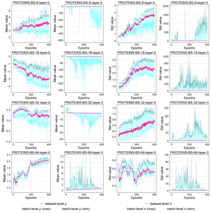
As Figure 4 in the main body, pink line denotes the dataset-level statistics, and green/blue line denotes the maximum/minimum value of the batch-level statistics respectively. First, we provide more results on PTC, NCI1, MUTAG, IMDB-BINARY tasks, as in Figure 8. We visualize the statistics from the first (layer-0) and the last (layer-3) BatchNorm layers in GIN for comparison. Second, we further visualize the statistics from different BatchNorm layers (layer 0 to layer 3) in GIN on PROTEINS and ResNet18 in CIFAR10, as in Figure 9. Third, we conduct experiments to investigate the influence of the batch size. We visualize the statistics from BatchNorm layers under different settings of batch sizes [8, 16, 32, 64], as in Figure 10. We can see that the observations are consistent and the batch statistics on graph data are noisy, as in Figure 4 in the main body.
D.3 Training Curves on GCN
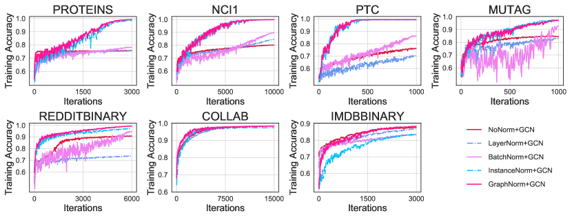
As Figure 2 in the main body, we train GCNs with different normalization methods (GraphNorm, InstanceNorm, BatchNorm and LayerNorm) and GCN without normalization in graph classification tasks and plot the training curves in Figure 6. It is obvious that the GraphNorm also enjoys the fastest convergence on all tasks. Remarkably, GCN with InstanceNorm even underperforms GCNs with other normalizations, while our GraphNorm with learnable shift significantly boosts the training upon InstanceNorm and achieves the fastest convergence.
D.4 Further Results of Ablation Study
BatchNorm with learnable shift.
We conduct experiments on BatchNorm to investigate whether simply introducing a learnable shift can already improve the existing normalization methods without concrete motivation of overcoming expressiveness degradation. Specifically, we equip BatchNorm with a similar learnable shift (-BatchNorm for short) as GraphNorm and evaluate its performance. As shown in Figure 12, the -BatchNorm cannot outperform the BatchNorm on the three datasets. Moreover, as shown in Figure 5 in the main body, the learnable shift significantly improve upon GraphNorm on IMDB-BINARY dataset, while it cannot further improve upon BatchNorm, which suggests the introduction of learnable shift in GraphNorm is critical.
BatchNorm with running statistics.
We study the variant of BatchNorm which uses running statistics (MS-BatchNorm for short) to replace the batch-level mean and standard deviation (similar idea is also proposed in Yan et al. (2019)). At first glance, this method may seem to be able to mitigate the problem of large batch noise. However, the running statistics change a lot during training, and using running statistics disables the model to back-propagate the gradients through mean and standard deviation. Thus, we also train GIN with BatchNorm which stops the back-propagation of the graidients through mean and standard deviation (DT-BatchNorm for short). As shown in Figure 12, both the MS-BatchNorm and DT-BatchNorm underperform the BatchNorm by a large margin, which shows that the problem of the heavy batch noise cannot be mitigated by simply using the running statistics.
The effect of batch size.
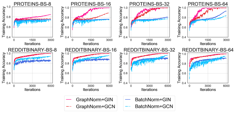
We further compare the GraphNorm and BatchNorm with different batch sizes (8, 16, 32, 64). As shown in Figure 11, our GraphNorm consistently outperforms the BatchNorm on all the settings.

Appendix E Other Related Works
Due to space limitations, we add some more related works on normalization and graph neural networks here. Zou et al. (2019) used normalization to stabilize the training process of GNNs. Zhao & Akoglu (2020) introduced PAIRNORM to prevent node embeddings from over-smoothing on the node classification task. Our GraphNorm focuses on accelerating the training and has faster convergence speed on graph classification tasks. Yang et al. (2020) interpreted the effect of mean subtraction on GCN as approximating the Fiedler vector. We analyze more general aggregation schemes, e.g., those in GIN, and understand the effect of the shift through the distribution of spectrum. Some concurrent and independent works (Li et al., 2020; Chen et al., 2020; Zhou et al., 2020b, a) also seek to incorporate normalization schemes in GNNs, which show the urgency of developing normalization schemes for GNNs. In this paper, we provide several insights on how to design a proper normalization for GNNs. Before the surge of deep learning, there are also many classic architectures of GNNs such as Scarselli et al. (2008); Bruna et al. (2013); Defferrard et al. (2016) that are not mentioned in the main body of the paper. We refer the readers to Zhou et al. (2018); Wu et al. (2020); Zhang et al. (2020) for surveys of graph representation learning.