Improving ERGM Starting Values Using Simulated Annealing

Abstract

Much of the theory of estimation for exponential family models, which include exponential-family random graph models (ERGMs) as a special case, is well-established and maximum likelihood estimates in particular enjoy many desirable properties. However, in the case of many ERGMs, direct calculation of MLEs is impossible and therefore methods for approximating MLEs and/or alternative estimation methods must be employed. Many MLE approximation methods require alternative estimates as starting points. We discuss one class of such alternatives here. The MLE satisfies the so-called “likelihood principle,” unlike the MPLE. This means that different networks may have different MPLEs even if they have the same sufficient statistics. We exploit this fact here to search for improved starting values for approximation-based MLE methods. The method we propose has shown its merit in producing an MLE for a network dataset and model that had defied estimation using all other known methods.

1 Maximum Likelihood Estimation for ERGMs

Given a network-valued random variable ${A}$ and a set of sufficient statistics ${T}:{\mathcal{A}}\to\mathbb{R}^{q}~{},~{}{a}\mapsto({T}_{1}(a),\dots,{T}_{q}(a))$, the exponential-family random graph model (ERGM) takes the form

$$P_{{\theta}}({A}={a})=\frac{\exp\left\{{\theta}^{\top}{T}({a})\right\}}{k({\theta})}\qquad\mbox{for ${a}\in{\mathcal{A}}$,}$$ (1)

where ${\mathcal{A}}$ is the sample space of allowable networks and ${\theta}\in\mathbb{R}^{q}$ is a vector of parameters. In many applications, ${\mathcal{A}}$ denotes the entire set $\{a\in\mathbb{R}^{N\times N},a_{ij}=a_{ji}\in\{0,1\},a_{ii}=0\}$ of possible undirected networks on $N$ nodes, while in other applications ${\mathcal{A}}$ may be constrained to be a proper subset of this set. (If we drop the requirement that $a_{ij}=a_{ji}$, then the sample space consists of directed networks.) The sufficient statistics ${T}({a})$ play a central role in the model, since they enable the inclusion of traditional exogenous covariates like a node’s age as well as endogenous statistics, i.e., statistics that allow for inference on the structure of the network. Popular endogenous statistics are a network’s number of triangles or the number of pairs of ties that share one common node (two-stars). The normalizing constant

$$k({\theta}):=\sum_{{a}^{*}\in{\mathcal{A}}}\exp\left\{{\theta}^{\top}T({a}^{*})\right\},$$ (2)

a weighted sum over all possible networks in the sample space, assures that (1) defines a probability model.

Maximizing the log-likelihood function

$$\ell({\theta})={\theta}^{\top}{T}({A^{\rm obs}})-\log k({\theta})$$ (3)

of the ERGM results in the maximum likelihood estimator, or MLE. The MLE can be difficult to calculate directly due to the required calculation of $k({\theta})$, a sum which is only feasible for particular choices of ${T}({a})$ for which the sum may be simplified or sample spaces small enough to allow direct calculation. Even for a small number of nodes, the sample space can be prohibitively large; for instance, there are over $3.5\times 10^{13}$ networks on just $N=10$ nodes, and an additional node inflates this number by a factor of over 1000. It is therefore often necessary to use an approximation method when an MLE is desired, as exact calculation is not possible.

An alternative method of estimation, known as maximum pseudolikelihood estimation (MPLE), has the desirable property that it is relatively easy to calculate even in cases where an exact MLE is elusive. This article first discusses approximate maximum likelihood estimation and then summarizes how MPLE works and explains why, even in cases where an MLE is desired, the approximation method often begins by calculating the MPLE. Then, in Section 4, we explain a novel method to augment the approximation of the MLE by exploiting the failure of the MPLE to satisfy the so-called likelihood principle. We demonstrate the use of this idea in Section 5.

2 Approximate MLE and Exact MPLE

An expedient to the problem of maximizing the often-intractable likelihood function (3) is given by the Markov chain Monte Carlo maximum likelihood estimator (MCMLE). First proposed by Geyer and Thompson (1992) and then adapted to the ERGM framework by Snijders (2002) and Hunter and Handcock (2006). The MCMLE is based on the idea that for any ${\theta}_{0}\in\mathbb{R}^{q}$,

$$\frac{k({\theta})}{k({\theta}_{0})}=\mathbb{E}_{{\theta}_{0}}\exp\left\{({\theta}-{\theta}_{0})^{\top}T({A})\right\},$$ (4)

where the expectation is taken assuming that the random ${A}$ has the distribution $P_{{\theta}_{0}}$.

For a given ${\theta}_{0}$, Equation (4) may be exploited by sampling a large number of networks $A_{1},\dots,A_{L}$ from the distribution $P_{{\theta}_{0}}$. Then one may approximate and optimize the difference of log-likelihood functions

$$\ell({\theta})-\ell({\theta}_{0})\approx({\theta}-{\theta}_{0})\cdot{T}({A})-\log\biggl{(}\frac{1}{L}\sum_{i=1}^{L}\exp\left\{({\theta}-{\theta}_{0})^{\top}{T}({A}_{i})\right\}\biggr{)}.$$ (5)

In theory, the MCMLE algorithm works for any starting value ${\theta}_{0}$, however, Hummel et al. (2012) show that approximation (5) is best when ${\theta}$ is close to ${\theta}_{0}$, and furthermore the approximation can degrade badly when these parameter values are not close. For this reason, in practice it is necessary to choose ${\theta}_{0}$ close to a maximizer of $\ell({\theta})$ or else the MCMLE idea fails.

The most common choice of ${\theta}_{0}$ is the maximizer of the so-called pseudolikellhood function. To construct the pseudolikelihood, we focus on the individual values of the tie indicators ${A}_{ij}$. A straightforward calculation shows that for a particular $i,j$, the conditional distribution of ${A}_{ij}$ given the rest of the network ${A}_{ij}^{c}$ is calculated from Equation (1) to be

$$P_{\theta}({A}_{ij}=1|{A}_{ij}^{c}={a}_{ij}^{c})=\mbox{logit}^{-1}\left[{\theta}^{\top}({T}({a}_{ij}^{+})-{T}({a}_{ij}^{-})\right],$$ (6)

where the inverse logit function is defined by $\mbox{logit}^{-1}(x)=\exp\{x\}/(1+\exp\{x\})$ and the networks ${a}_{ij}^{+}$ and ${a}_{ij}^{-}$ are formed by setting the value of ${a}_{ij}$ to be one or zero, respectively, while fixing the rest of the network at ${a}_{ij}^{c}$. We define $(\Delta{a})_{ij}:={T}({a}_{ij}^{+})-{T}({a}_{ij}^{-})$ and refer to $(\Delta{a})_{ij}$ as the $i,j$ vector of change statistics. We may therefore rewrite Equation (6) as

$$P_{\theta}({A}_{ij}=1|{A}_{ij}^{c}={a}_{ij}^{c})=\mbox{logit}^{-1}\left[{\theta}^{\top}(\Delta{a})_{ij}\right]$$

for all $i,j$. Under the additional assumption that the ${A}_{ij}$ are all independent of one another, these equations together define a logistic regression model, and the maximum likelihood estimator for this logistic regression is known as the maximum pseudo-likelihood estimator (MPLE) because the assumption of independence is not justified in all cases and therefore the logistic regression likelihood function is sometimes misspecified. Despite this misspecification, the MPLE is frequently used as an estimator of ${\theta}$ because it is easily obtained using logistic regression software. Indeed, the MPLE has a lengthy history in the literature on ERGMs; see Schmid and Hunter (2020) for more details.

In particular, there is a substantial literature on the use of MPLE as an estimator in its own right. For example, Schmid and Hunter (2020) argue that when its covariance is properly estimated, the MPLE can allow for valid statistical inference just as the MLE can. On the other hand, for the most part it is assumed (see, e.g., van Duijn et al., 2009) that MLE is preferable to MPLE. Indeed, one might prefer MLE to MPLE simply based on the classical principle, as articulated by John Tukey for example, “Far better an approximate answer to the right question, which is often vague, than an exact answer to the wrong question, which can always be made precise” (Tukey, 1962). For the purpose of this article, the MPLE will serve merely as a value ${\theta}_{0}$ used in Approximation (5) and we assume that the ultimate goal is to obtain an approximate MLE via MCMLE.

3 Comparison of MLE with MPLE

The theory of exponential family models is well-established in general; Barndorff-Nielsen (1978) gives an extensive book-length treatment of this theory. As a particularly useful example in the context of ERGMs, for exponential family distributions the expectation of the ${T}$ vector under the MLE equals the sufficient statistic on the observed network, i.e., $\mathbb{E}_{\hat{{\theta}}}[{T}({A})]={T}({A^{\rm obs}})$. In other words, the MLE equals the method of moments estimator. This aligns with one’s general expectation that the distribution described by an estimate should on average describe the observed network. Furthermore, this fact provides a useful means for checking that a potential maximizer of the approximate log-likelihood function is in fact close to the MLE, as one may simulate networks from the distribution derived from the MLE and check that their sample mean is approximately equal to ${T}({A^{\rm obs}})$.

3.1 The Likelihood Principle

Another property of the MLE is that it satisfies the likelihood principle (Barnard et al., 1962; Birnbaum, 1962), which states that all information in the data relevant to the model parameters is contained in the likelihood function. In the ERGM context, this means that an estimator should depend on ${A^{\rm obs}}$ only through ${T}({A^{\rm obs}})$, as the likelihood itself depends on ${A^{\rm obs}}$ only through ${T}({A^{\rm obs}})$. This means that two networks with the same sufficient statistic will yield the same MLE. However, as Corander et al. (1998) point out, the MPLE does not satisfy the likelihood principle. This observation forms the basis of the remainder of this article.

The failure of the MPLE to satisfy the likelihood principle means that two networks ${A}^{1}$ and ${A}^{2}$ may have different MPLEs even if ${T}({A}^{1})={T}({A}^{2})$. We see this fact illustrated in Figure  1, which depicts numerous possible MPLE values, each of which results from a network on 9 nodes with the same values of ${T}$. Also depicted in Figure 1 is the mean value parameter space, an alternative to the natural parameter space $\mathbb{R}^{q}$, which is defined as the interior of the sufficient statistic’s sample space. Each parameter ${\theta}$ can be uniquely projected to a point $g$ in mean value parameter space by a bijective function $\mu:\mathbb{R}^{q}\to\mathcal{C}$. For exponential family distributions, this function is defined as $\mu({\theta})=\nabla\log k({\theta})=\mathbb{E}_{{\theta}}[T(Y)]$. In other words, a parameter ${\theta}$’s corresponding point in mean value space is the expectation of the sufficient statistic with respect to the distribution defined by ${\theta}$. This means that ${T}({A^{\rm obs}})$ is the MLE’s projection into mean value parameter space, which is an interesting fact in its own right, since the MLE in natural parameter space is hard to find, but finding its counterpart in mean value space is trivially easy.

Figure 1: Every grey dot represents the MPLE of a network on $N=9$ nodes with 18 edges and 13 triangles using Model 7. The ’X’ visualizes the MLE.

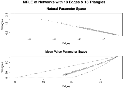
More specifically, Figure 1 depicts the MLE and multiple MPLEs in the natural as well as in mean value parameter space of networks on $N=9$ nodes with exactly $18$ edges and $13$ triangles. The dashed lines in the lower plot visualize the boundary of the convex hull of the mean value parameter space. The networks were sampled from the $(\rho,\sigma,\tau)$-model of Frank and Strauss (1986) with $\sigma$ taken to be zero, which results in an ERGM with a 2-dimensional ${T}$ vector. We fixed $\rho=-1$ and $\tau=0.53$, which is equivalent to

$$P_{{\theta}}({A}={a})\propto\exp\left\{-1\cdot(\mbox{\# edges})+0.53\cdot(\mbox{\# triangles})\right\}.$$ (7)

With only 9 nodes, it is computationally feasible to enumerate all possible $T({a})$ vectors for ${a}\in{\mathcal{A}}$, so it is possible to calculate the MLE exactly in this case. Schmid and Hunter (2020) demonstrate how to achieve this enumeration using the ergm package (Handcock et al., 2019) for the R computing environment (R Core Team, 2020). Although it is possible to enumerate all network statistics according to their multiplicity in this 9-node example, it is not computationally feasible to calculate every possible MPLE resulting from a network with 18 edges and 13 triangles. Thus, Figure 1 uses the simulated annealing method explained in Section 4 to generate multiple such networks randomly.

3.2 Rao-Blackwellization

Another potential way to exploit the failure of the MPLE to satisfy the likelihood principle is via the so-called Rao-Blackwellization of the MPLE. The Rao-Blackwell theorem (Lehmann and Casella, 1998) states that any estimator that is not a function of the sufficient statistic ${T}({a})$ is inadmissible, meaning that for any estimator $\tilde{{\theta}}$ that is not a function of ${T}({a})$, one can find an improved estimator ${\theta}^{*}$ by taking the expectation of $\tilde{{\theta}}$ conditional on ${T}({a})$. This new estimator has lower risk than $\tilde{{\theta}}$ by any convex lost function, e.g., mean squared error.

In principle, computing the Rao-Blackwellized MPLE would require the distribution of the MPLE conditional on ${T}({A^{\rm obs}})$. To put this idea into practice, a sample from this distribution could be obtained using, say, the simulated annealing method of Section 4. However, since the stochastic properties of the simulated annealing algorithm are not well understood, we have not explored this particular idea in the current manuscript.

4 New Starting Values Via Simulated Annealing

As described earlier, maximum likelihood estimation by MCMC requires the selection of an auxiliary parameter ${\theta}_{0}$. Even though in theory the algorithm operates with any choice of ${\theta}_{0}$, in practice, a parameter close to the MLE is essential for the MCMLE algorithm to work successfully (Hummel et al., 2012). The commonly used starting value for ${\theta}_{0}$ is the MPLE, since it is simple to calculate via logistic regression; even though other methods have been proposed (e.g., Krivitsky, 2017), MPLE remains the predominant method. As shown in Figure 1, however, the MPLE can in some cases be very different from the MLE, which typically results in the failure of the MCMLE algorithm. In our 9-node example, the MCMLE algorithm failed for about a third of the MPLEs as starting values shown in Figure 1.

4.1 Failure of the MCMLE algorithm: An Illustrative Example

Figure 2: A network with 18 edges and 13 triangles.

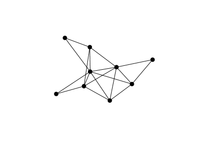
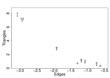
We demonstrate the problems of the MPLE as starting value for the MCMLE algorithm by taking a particular network on $9$ nodes with $18$ edges and $13$ triangles as depicted in Figure 2. The MPLE of this particular network is $\tilde{{\theta}}=(-1.3,0.702)$, while the MLE can be exactly calculated as $\hat{{\theta}}=(-0.623,0.337)$. Table 3 shows MCMLE results for the same network, where the algorithm was initialized by different $\tilde{{\theta}}$ values at each trial from among the values depicted in Figure 1. In four out of ten trials, the algorithm stopped due to model degeneracy. As first sketched by Handcock (2001) and later studied in detail by Schweinberger (2011), degeneracy occurs when the distribution defined by $P_{\hat{\theta}}$—ostensibly the best possible parameter value, in some sense—places most of its probability mass on just a few networks, usually the empty and the full network. In this scenario, the simulated networks are so different from the observed network that the MCMLE algorithm fails. In six cases shown in Table 3, the algorithm provided an MCMLE. Yet three trials yielded estimates further away from the MLE than the MPLE, leading to estimates in natural parameter space close to the boundary of the convex hull and therefore clearly different from the true MLE based on the observed network. The only glimmer of hope is trial 5, which leads to an estimate somewhat similar to the MLE. This example shows that it is necessary to check that an MLE is producing values of ${T}$, on average, close to ${T}({A^{\rm obs}})$. Once this takes place, additional techniques such as those detailed in Hummel et al. (2012) may be employed to fine-tune the MLE. However, even using such techniques, many of the trials from Table 3 did not end successfully.

Figure 3: MCMLEs of the network in Figure 2 using Model (7) for ten independent trials. ’+’ indicates the MPLE, ’x’ the MLE.

4.2 Simulated Annealing and MPLE

As noted earlier, Hummel et al. (2012) show that a poorly chosen ${\theta}_{0}$ can make successful MCML estimation almost impossible. Consequently, the more different the MPLE is from the MLE, the more difficult it is to find the MCMLE, since the MPLE is commonly taken as the algorithm’s starting value ${\theta}_{0}$ due to its simple and fast calculation. Inspired by Figure 1, we propose a novel approach for finding an improved starting value for the MCMLE algorithm, namely, to search for networks that yield the same—or at least nearly the same— statistics as the observed network, then consider these networks’ MPLEs as potential starting values.

We propose searching for networks with the same statistics as the observed network using the simulated annealing algorithm (Kirkpatrick et al., 1983). This algorithm was initially inspired from the practice of annealing metal, a procedure in which the material is heated and then cooled very slowly, allowing it to be gradually shaped into the desired form. The process of heating up and cooling down is translated into the simulated annealing approach by allowing interim results initially (during the “heated” phase) to be worse than previous results; that is, the algorithm is more stochastic than deterministic in its early phase. Gradually, the algorithm “cools,” becoming more deterministic and less prone to random jumps. The hope is that the algorithm does not get stuck at local maxima that it otherwise might not be able to leave if a purely deterministic optimization algorithm were used. By starting in an initial random phase followed by increasingly deterministic behavior, the algorithm can find and then focus on areas of the search space that include globally optimal solutions.

5 Applications

We demonstrate the simulated annealing-based approach to MCMLE using the E. coli transcriptional regulation network of Shen-Orr et al. (2002), which is based on the RegulonDB data of Salgado et al. (2001). The nodes in this network represent operons, while an edge from operon $i$ to $j$ indicates that $i$ encodes a transcription factor that regulates $j$. Even though this is originally a directed network that contains self-edges, i.e., operons that regulate themselves, we follow Saul and Filkov (2007) and treat this network as undirected and without self-edges. This results in a network with 519 edges and 418 nodes. We study the same ERGM on these data as Hummel et al. (2012), a model which yields MCMLEs considerably different from the MPLE, making estimation difficult. The model’s statistics consist of the number of edges; the numbers of nodes with degrees two, three, four, and six; and the geometrically weighted degree distribution with the decay parameter fixed at $0.25$. As demonstrated by Hummel et al. (2012), initializing the MCMLE algorithm with the MPLE does not produce successful results.

Figure 4: MPLEs of networks with the same sufficient statistics as the observed E. coli network. The MPLE of the observed network is marked with an ’+’, the MCMLE with an ’x’.

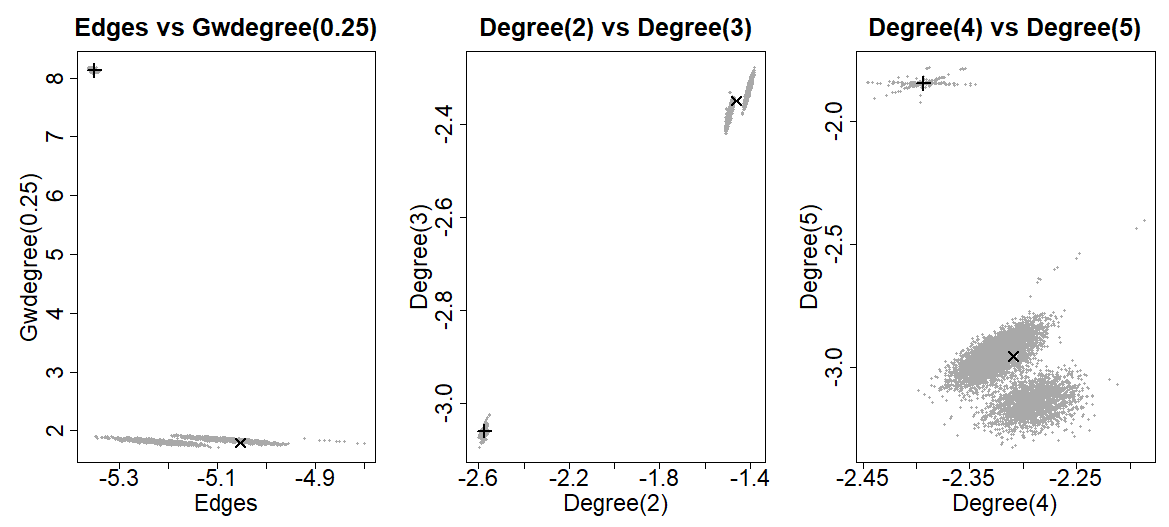
Figure 4 depicts the MPLEs of 10,000 networks (in grey) that have the same sufficient statistics as the original network, including the MPLE of the original network as well as the MCMLE. All $10,000$ networks were obtained using the simulated annealing algorithm, always starting with the observed network. It is remarkable that the MPLEs of these networks essentially form two clusters, one cluster that includes the MPLE and another one that includes the MCMLE of the observed network. Among other things, this figure illustrates why finding the MCMLE by beginning the algorithm at the observed network’s MPLE is a difficult task. The MPLE is simply not close enough to the MLE for the approximate log-likelihood using an MPLE-based sample of networks to be effective. On the other hand, setting the starting value to one of the MPLEs that form the cluster around the MCMLE evidently makes the algorithm more likely to succeed.

A natural question that arises when considering Figure 4 is how the networks in the two clusters differ. Figure 5 visualizes networks of each cluster as well as the original E. coli network. Even though all three networks have the same sufficient statistics, it is possible to discern that the network in the MPLE cluster maintains some of the distinctive structures of the original network, while the network in the MCMLE cluster is more reminiscent of an Erdös-Rényi network, i.e., a network where each tie occurs independently with same probability $p$. The fact that the occurrence of a tie in an Erdös-Rényi network does not depend on the occurrence or absence of any other tie results in a model in which the MPLE and the MLE are the same. Consequently, we conjecture that it is advantageous to find a network that resembles an Erdös-Rényi network and that, in addition, yields the same sufficient statistics as the observed network.

Figure 5: The left visualizes the E.coli transcriptional regulation network of Shen-Orr et al. (2002). The center depicts a network whose MPLE falls into the MPLE cluster of Figure 4. The right depicts a network whose MPLE falls into the MPLE cluster of Figure 4. All three networks have the same sufficient statistics vector.

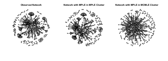
Simulating networks from the probability distribution defined by the obtained MCMLE results in networks that resemble the rightmost network in Figure 5, rather than the observed network. This consequently casts doubt on whether the statistics of this ERGM appropriately capture the unique structure of the observed network. Stated differently, if the MLE, ostensibly the gold standard among estimators, yields unsatisfying results, the model itself should be reconsidered. It is important to remember that in such cases, as indeed in this case, generally the MPLE also fails to result in simulated networks resembling the original network; thus, a poor model cannot generally be mended by using a different estimation technique.

We repeat the simulation study that resulted in Figure 4, with the exception that we start the simulated annealing algorithm with an Erdös-Rényi-generated network with similar density to the original network, i.e., where $p$ is defined as the ratio of the number of ties to the number of possible ties. With this modification, the simulated annealing algorithm only finds networks where the MPLE is in the proximity of the MCMLE, meaning that the MPLE of any of these networks is an improved starting value for the MCMLE algorithm compared to the original MPLE.

In summary, we suggest finding an improved starting value ${\theta}_{0}$ the following way:

1. For a given network ${A^{\rm obs}}$, find the sufficient statistics ${T}({A^{\rm obs}})$

2. Simulate a network $G$ using an Erdös-Rényi model on the same nodes as ${A^{\rm obs}}$ and with $p$ given by the edge density of ${A^{\rm obs}}$

3. Simulate a new network ${A}^{*}$ with ${T}({A}^{obs})={T}({A}^{*})$ with simulated annealing and start with the algorithm at $G$. If ${T}({A})$ includes continuous statistics, find a network $A^{*}$ with ${T}({A})\approx{T}({A}^{*})$

4. Take the MPLE of $A^{*}$ as the improved starting value ${\theta}_{0}$

This approach was successfully applied by Schmid et al. (2020) to a citation network based on all US Supreme Court majority opinions written between 1937 and 2015. The majority opinion of each court case is considered a node, and a citation from case $i$ to case $j$ is defined as a directed tie. The network includes $10{,}020$ nodes and the ERGM used includes $14$ endogenous and exogenous statistics—complicated enough to be computationally challenging. Ultimately, Schmid et al. (2020) find that multiple different approaches fail to yield a successful MCMLE, among them the stepping method of Hummel et al. (2012) and the standard MCMLE algorithm using the MPLE as starting value. Yet the approach described here—which reproduces the observed network statistics only approximately due to the inclusion of several continuous variables among these statistics—does produce a successful MCMLE; it is the only known method that does so in this example.

6 Discussion

The basic idea of this article—searching for networks that have the same, or approximately the same, ERGM statistics as the observed network and then using the MPLEs from these networks as starting values for a traditional MCMLE algorithm—is relatively simplistic. Yet it has already demonstrated its value in solving previously unsolvable ERGM-based estimation problems.

It seems there is still much to learn about this methodology. For instance, is there a way to implement Rao-Blackwellization, and does this approach lead to estimates that are closer in their behavior to the MLE? Also, how important is it to search the sample space of all networks thoroughly, and is an alternative to simulated annealing possible for this purpose? Figure 4 suggests that initializing the simulated annealing algorithm at the observed network and the Erdös-Rényi-generated network generate wholly distinct clouds of MPLE values, which leads to the question of whether all possible MPLE values for a particular set of statistics is actually bimodal, or whether in fact there is a vast as-yet-unexplored set of MPLE values that could potentially be of use both as starting MCMLE values and as sample points in a Rao-Blackwellization scheme.

That such a simple idea can prove so effective relative to all other known methods suggests that there exists immense untapped potential for improving upon approximate likelihood-based inference using MPLEs.

References

- Barnard et al. (1962) Barnard, G. A., G. M. Jenkins, and C. B. Winsten (1962). Likelihood inference and time series. Journal of the Royal Statistical Society. Series A (General) 125(3), 321–372.
- Barndorff-Nielsen (1978) Barndorff-Nielsen, O. (1978). Information and Exponential Families in Statistical Theory. Wiley.
- Birnbaum (1962) Birnbaum, A. (1962). On the foundations of statistical inference. Journal of the American Statistical Association 57(298), 269–306.
- Corander et al. (1998) Corander, J., K. Dahmström, and P. Dahmström (1998). Maximum likelihood estimation for Markov graphs. Technical report, Department of Statistics, University of Stockholm.
- Frank and Strauss (1986) Frank, O. and D. Strauss (1986). Markov graphs. Journal of the American Statistical Association 81(395), 832–842.
- Geyer and Thompson (1992) Geyer, C. J. and E. A. Thompson (1992). Constrained Monte Carlo maximum likelihood for dependent data. Journal of the Royal Statistical Society. Series B (Methodological) 54(3), 657–699.
- Handcock (2001) Handcock, M. S. (2001). Assessing degeneracy in statistical models of social networks. Technical report, Center for Statistics and the Social Sciences, University of Washington.
- Handcock et al. (2019) Handcock, M. S., D. R. Hunter, C. T. Butts, S. M. Goodreau, P. N. Krivitsky, and M. Morris (2019). ergm: Fit, Simulate and Diagnose Exponential-Family Models for Networks. The Statnet Project (https://statnet.org). R package version 3.10.0-4837.
- Hummel et al. (2012) Hummel, R. M., D. R. Hunter, and M. S. Handcock (2012). Improving simulation-based algorithms for fitting ERGMs. Journal of Computational and Graphical Statistics 21(4), 920–939.
- Hunter and Handcock (2006) Hunter, D. R. and M. S. Handcock (2006). Inference in curved exponential family models for networks. Journal of Computational and Graphical Statistics 15(3), 565–583.
- Kirkpatrick et al. (1983) Kirkpatrick, S., C. D. Gelatt, and M. P. Vecchi (1983). Optimization by simulated annealing. Science 220(4598), 671–680.
- Krivitsky (2017) Krivitsky, P. N. (2017). Using contrastive divergence to seed Monte Carlo MLE for exponential-family random graph models. Computational Statistics and Data Analysis 107(C), 149–161.
- Lehmann and Casella (1998) Lehmann, E. and G. Casella (1998). Theory of Point Estimation. Springer Verlag.
- R Core Team (2020) R Core Team (2020). R: A Language and Environment for Statistical Computing. Vienna, Austria: R Foundation for Statistical Computing.
- Salgado et al. (2001) Salgado, H., A. Santos-Zavaleta, S. Gama-Castro, D. Millán-Zárate, E. Díaz-Peredo, F. Sánchez-Solano, E. Pérez-Rueda, C. Bonavides-Martínez, and J. Collado-Vides (2001). RegulonDB (version 3.2): Transcriptional regulation and operon organization in Escherichia coli K-12. Nucleic acids research 29(1), 72–74.
- Saul and Filkov (2007) Saul, Z. and V. Filkov (2007). Exploring biological network structure using exponential random graph models. Bioinformatics (Oxford, England) 23, 2604–11.
- Schmid et al. (2020) Schmid, C. S., T. H. Chen, and B. A. Desmarais (2020). Generative dynamics of Supreme Court citations. Working Paper, The Pennsylvania State University.
- Schmid and Hunter (2020) Schmid, C. S. and D. R. Hunter (2020). Accounting for model misspecification when using pseudolikelihood for ERGMs. Unpublished manuscript.
- Schweinberger (2011) Schweinberger, M. (2011). Instability, sensitivity, and degeneracy of discrete exponential families. Journal of the American Statistical Association 106(496), 1361–1370.
- Shen-Orr et al. (2002) Shen-Orr, S., R. Milo, S. Mangan, and U. Alon (2002, 06). Network motifs in the transcriptional regulation network of Escherichia coli. Nature genetics 31, 64–68.
- Snijders (2002) Snijders, T. A. (2002). Markov chain Monte Carlo estimation of exponential random graph models. Journal of Social Structure 3(2), 1–40.
- Tukey (1962) Tukey, J. W. (1962). The future of data analysis. Annals of Mathematical Statistics 33, 1–67.
- van Duijn et al. (2009) van Duijn, M. A., K. J. Gile, and M. S. Handcock (2009). A framework for the comparison of maxmimum pseudo-likelikood and maximum likelihood estimation of exponential family random graph models. Social Networks 31(1), 52–62.