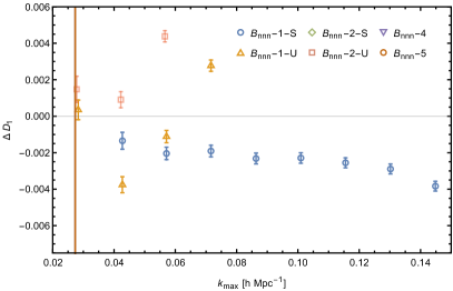
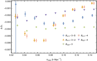
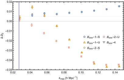
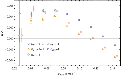
Precise Calibration of the One-Loop Bispectrum in the Effective Field Theory of Large Scale Structure

Theodore Steele ts715@cam.ac.uk Department of Applied Mathematics and Theoretical Physics, University of Cambridge    Tobias Baldauf Department of Applied Mathematics and Theoretical Physics, University of Cambridge
Abstract

The bispectrum is the leading non-Gaussian statistic in Large-Scale Structure (LSS) clustering and encodes the interactions in the underlying field. It is thus an important diagnostic for primordial non-Gaussianity and higher order galaxy biasing. In this paper we present a detailed test and calibration of the matter bispectrum counterterms in the Effective Field Theory of LSS against a suite of N𝑁N-body simulations. We are going beyond previous studies in employing realisation based perturbation theory that allows for a significant reduction in cosmic variance error bars. This enables the measurement of the low-energy constants on large scales before two-loop corrections become relevant, around k<0.09hMpc1𝑘0.09superscriptMpc1k<0.09h\ \text{Mpc}^{-1} at z=0𝑧0z=0. We also go beyond previous work in using bispectrum propagator terms, i.e. correlators with linear and second order fields, to quantify the two new counterterms in isolation and to establish consistency with the power spectrum counterterm. By investigating the fully non-linear bispectrum, Bnnnsubscript𝐵nnnB_{\mathrm{nnn}}, as well as the terms Bn11subscript𝐵n11B_{\mathrm{n}11} and Bn21subscript𝐵n21B_{\mathrm{n}21}, we find evidence for the new counterterms deviating from the shape suggested by the UV-limit of the relevant bispectrum contributions. We also show that the commonly used Einstein-de Sitter approximation for the time dependence of the tree-level bispectrum is insufficient for precise studies of the one-loop bispectrum and that it is necessary to use ΛΛ\LambdaCDM growth factors in order to obtain meaningful one-loop counterterm constraints. Finally, we also find evidence for small deviations in the growth factors that arise from time integration inaccuracies in the N𝑁N-body simulations.

I Introduction

Cosmological probes are observables that can be used to constrain the parameter space of fundamental theories; examples include the Cosmic Microwave Background (CMB) Aghanim et al. (2018); Akrami et al. (2018) and the distribution of matter and galaxies across the universe, known as cosmological Large-Scale Structure (LSS). Since its discovery, the CMB has proven to be a rich source of cosmological information. While it has provided many valuable insights and tight parameter constraints on the ΛΛ\LambdaCDM model, its statistical power has been mostly exhausted. Yet many open questions remain, such as the mass of neutrinos or the dynamics and field content of inflation. LSS offers to provide significantly more information than the CMB on account of its three dimensional nature. However, modelling LSS is more difficult than modelling the CMB due to non-linearities in the late-time Universe.

Until the beginning of the last decade, there was a strong ambition to describe LSS in a parameter free, deterministic approach referred to as Standard Perturbation Theory (SPT) Bernardeau et al. (2002). This model is based on a fluid approximation to the Vlaslov equation describing an ensemble of collisionless particles and solves the equations perturbatively using a power series in the density and velocity divergence fields. However, the results of SPT beyond tree-level are in tension with simulations as SPT does not take into account the small-scale effects of gravitational collapse. These cannot be described perturbatively and, through their resultant effects on the gravitational field, lead to non-perturbative effects on cosmic structure at larger scales.

To solve this problem, a modification to SPT, called the Effective Field Theory of Large Scale Structure (EFTofLSS) Baumann et al. (2012); Carrasco et al. (2012); Carrasco et al. (2014a); Pajer and Zaldarriaga (2013), has been developed. The EFTofLSS introduces an arbitrarily chosen coarse graining or regulation scale ΛΛ\Lambda that allows for a convergent series expansion for wavenumbers below the non-linear wavenumber kNLsubscript𝑘NLk_{\text{NL}}, beyond which physics is non-perturbative. The coarse grained equations of motion are now ΛΛ\Lambda-dependent and contain an effective stress term that encapsulates microscopic velocity dispersion and products of small scale modes. As these effects are non-perturbative, they need to be parametrised in a broad manner that allows for all operators that are compatible with the symmetries of the model. The new terms this introduces into the perturbative expansion are called counterterms and account for small scale deviations from the pressureless perfect fluid assumed by SPT, absorbing divergences and the dependence on ΛΛ\Lambda, making the overall model cutoff independent.

Recently, the potential of the EFTofLSS to deliver unbiased cosmological constraints has been proven in a blind analysis of a simulation suite Nishimichi et al. (2020). The same approach has then been used to perform an analysis of galaxy correlators in the BOSS survey Ivanov et al. (2020); D’Amico et al. (2020), which can be connected to the overall matter and dark matter correlators by taking into account the appropriate biasing terms. The latter account for the fact that the galaxy distribution correlates with but does not perfectly mimic the underlying dark matter distribution Desjacques et al. (2018).

A lot of attention has been devoted to the EFT at the level of the power spectrum Carrasco et al. (2012); Carrasco et al. (2014a); Baldauf et al. (2015a), the two-point correlator and therefore the simplest statistic in LSS, while less attention has been devoted to the bispectrum Angulo et al. (2015); Baldauf et al. (2015b) and trispectrum Bertolini et al. (2016a, b). The galaxy bispectrum at one-loop has recently been studied in Eggemeier et al. (2019). The higher order statistics offer additional information as well as the opportunity to perform consistency checks with the EFT parameters calculated from the power spectrum. Further tests of the EFT bispectrum have also been performed in Lazanu et al. (2016) and their calculations have been pushed to two-loop order in Lazanu and Liguori (2018). We improve upon these results by implementing the full ΛΛ\LambdaCDM time dependence rather than the commonly employed Einstein-de Sitter approximation for cosmological perturbation theory and cancelling cosmic variance through realisation perturbation theory. We analyse the effects of these corrections for the power spectrum, auto bispectrum, and bispectrum propagators.

This paper will use a simulation suite previously studied in Baldauf et al. (2015b, a). It is based on a Ωm,0=0.272subscriptΩm,00.272\Omega_{\text{m,0}}=0.272, σ8=0.81subscript𝜎80.81\sigma_{8}=0.81, ns=0.967subscript𝑛s0.967n_{\text{s}}=0.967 cosmology with h=0.7240.724h=0.724. The Np=10243subscript𝑁psuperscript10243N_{\text{p}}=1024^{3} particles in a cubic box of dimension L=1500h1Mpc𝐿1500superscript1MpcL=1500h^{-1}\ \text{Mpc} are set up at initial redshift zi=99subscript𝑧i99z_{\text{i}}=99 using 2LPT Crocce et al. (2006) and then evolved to z=0𝑧0z=0 using Gadget 2 Springel (2005). We are considering 14 realisations of this simulation volume. The realization perturbation theory approach has previously been used to evaluate and test SPT Roth and Porciani (2011); Taruya et al. (2018, 2020), but not to our knowlegde to constrain the EFT counterterms.

This paper is structured as follows: We first review the EFT and the corresponding counterterms in Sec. II, before reviewing the power spectrum and bispectrum as well as their ΛΛ\LambdaCDM time dependence and our realisation perturbation theory implementation in Sec. II.6. We then explain the various fitting procedures we used to estimate the counterterm amplitudes before presenting parameter constraints in Sec. III. We finally conclude and offer a discussion of our various results and their implications in Sec. IV.

II Perturbative Modelling of the Bispectrum

II.1 The Effective Field Theory

Cosmological perturbation theory is based on an ensemble of N𝑁N collisionless point particles Bernardeau et al. (2002) whose overall phase space density is given by f(𝐱,𝐩)=i=1Nfi(𝐱,𝐩)𝑓𝐱𝐩superscriptsubscript𝑖1𝑁subscript𝑓𝑖𝐱𝐩f(\mathbf{x},\mathbf{p})=\sum_{i=1}^{N}f_{i}(\mathbf{x},\mathbf{p}), where 𝒑𝒑\bm{p} is the canonical momentum and fi(𝐱,𝐩)=δ(D)(𝐱𝐱i)δ(D)(𝐩ma𝐯i)subscript𝑓𝑖𝐱𝐩superscript𝛿(D)𝐱subscript𝐱𝑖superscript𝛿(D)𝐩𝑚𝑎subscript𝐯𝑖f_{i}(\mathbf{x},\mathbf{p})=\delta^{\text{(D)}}(\mathbf{x}-\mathbf{x}_{i})\delta^{\text{(D)}}(\mathbf{p}-ma\mathbf{v}_{i}). Such an ensemble obeys the collisionless Boltzmann equation

DfDt=ft+𝐩ma2f𝐱mϕ𝐱f𝐩=0,D𝑓D𝑡𝑓𝑡𝐩𝑚superscript𝑎2𝑓𝐱𝑚italic-ϕ𝐱𝑓𝐩0\frac{\text{D}f}{\text{D}t}=\frac{\partial f}{\partial t}+\frac{\mathbf{p}}{ma^{2}}\cdot\frac{\partial f}{\partial\mathbf{x}}-m\frac{\partial\phi}{\partial\mathbf{x}}\cdot\frac{\partial f}{\partial\mathbf{p}}=0~{}\,, (1)

where ϕitalic-ϕ\phi is the gravitational potential. We coarse grain the phase space by introducing a smoothing function, WΛ(k)subscript𝑊Λ𝑘W_{\Lambda}(k). The presence of this function differentiates the EFT from SPT, and it is defined by

WΛ(k)=e12k2Λ2,subscript𝑊Λ𝑘superscript𝑒12superscript𝑘2superscriptΛ2W_{\Lambda}(k)=e^{-\frac{1}{2}\frac{k^{2}}{\Lambda^{2}}}~{}, (2)

for some cutoff Λ<kNLΛsubscript𝑘NL\Lambda<k_{\text{NL}}. Here kNLsubscript𝑘NLk_{\text{NL}} is the non-linear scale beyond which the physics is non-perturbative. Throughout this paper we choose Λ=0.3hMpc1Λ0.3superscriptMpc1\Lambda=0.3h\ \text{Mpc}^{-1} unless explicitly stated otherwise. Note that the theory is independent of the cutoff and that the need for an explicit cutoff is of a numerical nature as discussed in detail below in Sec. II.7.

Taking the first two moments of Eq. (1) gives us definitions for the matter and momentum densities,

ρ(𝐱,τ)=ma3d3yd3qWΛ(𝐱𝐲)f(𝐲,𝐩)𝜌𝐱𝜏𝑚superscript𝑎3superscriptd3𝑦superscript𝑑3𝑞subscript𝑊Λ𝐱𝐲𝑓𝐲𝐩\rho(\mathbf{x},\tau)=\frac{m}{a^{3}}\int\text{d}^{3}y\int d^{3}q~{}W_{\Lambda}(\mathbf{x}-\mathbf{y})~{}f(\mathbf{y},\mathbf{p}) (3)

and

𝝅(𝐱,τ)=1a4d3yd3𝐩WΛ(𝐱𝐲)𝐩f(𝐲,𝐩).𝝅𝐱𝜏1superscript𝑎4superscriptd3𝑦superscript𝑑3𝐩subscript𝑊Λ𝐱𝐲𝐩𝑓𝐲𝐩\bm{\pi}(\mathbf{x},\tau)=\frac{1}{a^{4}}\int\text{d}^{3}y\int d^{3}\mathbf{p}~{}W_{\Lambda}(\mathbf{x}-\mathbf{y})~{}\mathbf{p}~{}f(\mathbf{y},\mathbf{p})~{}. (4)

Applying these to the Boltzmann equation allows us to derive the equations of motion

ρ˙+3Hρ+1ai(ρvi)=0˙𝜌3𝐻𝜌1𝑎subscript𝑖𝜌superscript𝑣𝑖0\dot{\rho}+3H\rho+\frac{1}{a}\partial_{i}(\rho v^{i})=0 (5)

and

v˙i+Hvi+1avjjvi+1aiϕ=1aρj[τij]Λ,superscript˙𝑣𝑖𝐻superscript𝑣𝑖1𝑎superscript𝑣𝑗subscript𝑗superscript𝑣𝑖1𝑎subscript𝑖italic-ϕ1𝑎𝜌subscript𝑗subscriptdelimited-[]superscript𝜏𝑖𝑗Λ\dot{v}^{i}+Hv^{i}+\frac{1}{a}v^{j}\partial_{j}v^{i}+\frac{1}{a}\partial_{i}\phi=-\frac{1}{a\rho}\partial_{j}[\tau^{ij}]_{\Lambda}, (6)

where x˙=tx˙𝑥subscript𝑡𝑥\dot{x}=\partial_{t}x, H=a˙/a𝐻˙𝑎𝑎H=\dot{a}/a is the Hubble rate, 𝐯=𝝅/ρ+counterterms𝐯𝝅𝜌counterterms\mathbf{v}=\bm{\pi}/\rho+\mathrm{counterterms} is the fluid velocity Mercolli and Pajer (2014), and the stress-energy tensor τijsuperscript𝜏𝑖𝑗\tau^{ij} describes the non-perturbative effects of small scale physics. The stress-energy tensor is set to zero in SPT. Taking the derivative of Eq. (6) and defining the velocity divergence field θ=ivi𝜃subscript𝑖superscript𝑣𝑖\theta=\partial_{i}v^{i}, we obtain

ηθ+θ+vjjθ+ivjjvi+ϕ=τθ,subscript𝜂𝜃𝜃superscript𝑣𝑗subscript𝑗𝜃subscript𝑖superscript𝑣𝑗subscript𝑗superscript𝑣𝑖italic-ϕsubscript𝜏𝜃\partial_{\eta}\theta+\mathcal{H}\theta+v^{j}\partial_{j}\theta+\partial_{i}v^{j}\partial_{j}v^{i}+\triangle\phi=\tau_{\theta}~{}, (7)

where η𝜂\eta is the conformal time defined through adη=dt𝑎d𝜂d𝑡a\text{d}\eta=\text{d}t and

τθ=i[1ρjτij].subscript𝜏𝜃subscript𝑖delimited-[]1𝜌subscript𝑗superscript𝜏𝑖𝑗\tau_{\theta}=-\partial_{i}\left[\frac{1}{\rho}\partial_{j}\tau^{ij}\right]\,. (8)

Defining the density contrast δ=ρ/ρ¯1𝛿𝜌¯𝜌1\delta=\rho/\bar{\rho}-1, Eq. (5) becomes

ηδ+[(1+δ)vi]=0.subscript𝜂𝛿delimited-[]1𝛿superscript𝑣𝑖0\partial_{\eta}\delta+\nabla\cdot\left[\left(1+\delta\right)v^{i}\right]=0~{}. (9)

Rewriting Eqs. (6) and (9) in Fourier space gives us

ηδ(𝐤,η)+θ(𝐤,η)=𝒮α(𝐤,η),subscript𝜂𝛿𝐤𝜂𝜃𝐤𝜂subscript𝒮𝛼𝐤𝜂\partial_{\eta}\delta(\mathbf{k},\eta)+\theta(\mathbf{k},\eta)=\mathcal{S}_{\alpha}(\mathbf{k},\eta), (10)

and

ηθ(𝐤,η)+θ(𝐤,η)+32Ωm2δ(𝐤,η)=𝒮β(𝐤,η).subscript𝜂𝜃𝐤𝜂𝜃𝐤𝜂32subscriptΩmsuperscript2𝛿𝐤𝜂subscript𝒮𝛽𝐤𝜂\partial_{\eta}\theta(\mathbf{k},\eta)+\mathcal{H}\theta(\mathbf{k},\eta)+\frac{3}{2}\Omega_{\mathrm{m}}\mathcal{H}^{2}\delta(\mathbf{k},\eta)=\mathcal{S}_{\beta}(\mathbf{k},\eta)~{}. (11)

The two non-linear source terms Sαsubscript𝑆𝛼S_{\alpha} and Sβsubscript𝑆𝛽S_{\beta} may be defined as

Sα(𝐤,η)=d3𝐩(2π)3α(𝐪,𝐤𝐪)θ(𝐪,η)δ(𝐤𝐪,η),subscript𝑆𝛼𝐤𝜂superscriptd3𝐩superscript2𝜋3𝛼𝐪𝐤𝐪𝜃𝐪𝜂𝛿𝐤𝐪𝜂S_{\alpha}(\mathbf{k},\eta)=-\int\frac{\mathrm{d}^{3}\mathbf{p}}{(2\pi)^{3}}\alpha(\mathbf{q},\mathbf{k}-\mathbf{q})\theta(\mathbf{q},\eta)\delta(\mathbf{k}-\mathbf{q},\eta)~{}, (12)
Sβ(𝐤,η)=d3𝐩(2π)3β(𝐪,𝐤𝐪)θ(𝐪,η)θ(𝐤𝐪,η)+τθ(𝐤,η).subscript𝑆𝛽𝐤𝜂superscriptd3𝐩superscript2𝜋3𝛽𝐪𝐤𝐪𝜃𝐪𝜂𝜃𝐤𝐪𝜂subscript𝜏𝜃𝐤𝜂S_{\beta}(\mathbf{k},\eta)=-\int\frac{\mathrm{d}^{3}\mathbf{p}}{(2\pi)^{3}}\beta(\mathbf{q},\mathbf{k}-\mathbf{q})\theta(\mathbf{q},\eta)\theta(\mathbf{k}-\mathbf{q},\eta)+\tau_{\theta}(\mathbf{k},\eta)~{}. (13)

The kernels α𝛼\alpha and β𝛽\beta encapsulating the coupling between modes are defined as

α(𝐤1,𝐤2)=𝐤1(𝐤1+𝐤2)k12𝛼subscript𝐤1subscript𝐤2subscript𝐤1subscript𝐤1subscript𝐤2superscriptsubscript𝑘12\alpha(\mathbf{k}_{1},\mathbf{k}_{2})=\frac{\mathbf{k}_{1}\cdot(\mathbf{k}_{1}+\mathbf{k}_{2})}{k_{1}^{2}} (14)

and

β(𝐤1,𝐤2)=12(𝐤1+𝐤2)2𝐤1𝐤2k12k22.𝛽subscript𝐤1subscript𝐤212superscriptsubscript𝐤1subscript𝐤22subscript𝐤1subscript𝐤2superscriptsubscript𝑘12superscriptsubscript𝑘22\beta(\mathbf{k}_{1},\mathbf{k}_{2})=\frac{1}{2}(\mathbf{k}_{1}+\mathbf{k}_{2})^{2}\frac{\mathbf{k}_{1}\cdot\mathbf{k}_{2}}{k_{1}^{2}k_{2}^{2}}\,. (15)

We can solve the equations of motion using a power series ansatz δn(𝒌,a)=Dnδn(𝒌)subscript𝛿𝑛𝒌𝑎subscript𝐷𝑛subscript𝛿𝑛𝒌\delta_{n}(\bm{k},a)=D_{n}\delta_{n}(\bm{k}) for growth factor Dnsubscript𝐷𝑛D_{n}, where in a matter dominated universe we simply have Dn=ansubscript𝐷𝑛superscript𝑎𝑛D_{n}=a^{n}. The n𝑛n-th order density field is given by

δn(𝐤)=𝐪1Λ𝐪nΛδ(D)(𝐤i=1n𝐪i)Fn(𝐪1,,𝐪n)i=1nδ1(𝐪i),subscript𝛿n𝐤superscriptsubscriptsubscript𝐪1Λsuperscriptsubscriptsubscript𝐪nΛsuperscript𝛿(D)𝐤superscriptsubscript𝑖1𝑛subscript𝐪𝑖subscript𝐹nsubscript𝐪1subscript𝐪nsuperscriptsubscriptproduct𝑖1𝑛subscript𝛿1subscript𝐪𝑖\delta_{\mathrm{n}}(\mathbf{k})=\int_{\mathbf{q}_{1}}^{\Lambda}\cdots\int_{\mathbf{q}_{\mathrm{n}}}^{\Lambda}\delta^{\text{(D)}}\Biggl{(}\mathbf{k}-\sum_{i=1}^{n}\mathbf{q}_{i}\Biggr{)}F_{\mathrm{n}}(\mathbf{q}_{1},...,\mathbf{q}_{\mathrm{n}})\prod_{i=1}^{n}\delta_{1}(\mathbf{q}_{i})~{}, (16)

where 𝐪=d3𝐪/(2π)3subscript𝐪superscriptd3𝐪superscript2𝜋3\int_{\mathbf{q}}=\int\text{d}^{3}\mathbf{q}/(2\pi)^{3} and the functions of momenta Fnsubscript𝐹nF_{\mathrm{n}} are the gravitational coupling kernels of the density field. The corresponding coupling kernels for the velocity divergence are referred to as Gnsubscript𝐺𝑛G_{n}. The Fnsubscript𝐹𝑛F_{n} and Gnsubscript𝐺𝑛G_{n} kernels are given by the recursion relations

Fn(𝐤1,,𝐤n)=subscript𝐹nsubscript𝐤1subscript𝐤nabsent\displaystyle F_{\mathrm{n}}(\mathbf{k}_{1},...,\mathbf{k}_{\mathrm{n}})= m=1n1Gm(𝐤1,,𝐤m)(2n+3)(n1)[(2n+1)α(κ1m,κm+1n)Fnm(𝐤m+1,,𝐤n)\displaystyle\sum^{n-1}_{m=1}\frac{G_{m}(\mathbf{k}_{1},...,\mathbf{k}_{m})}{(2n+3)(n-1)}[(2n+1)\alpha(\mathbf{\kappa}_{1}^{m},\mathbf{\kappa}_{m+1}^{n})F_{\mathrm{n}-m}(\mathbf{k}_{m+1},...,\mathbf{k}_{\mathrm{n}})
+2β(κ1m,κm+1n)Gnm(𝐤m+1,,𝐤n)],\displaystyle+2\beta(\mathbf{\kappa}_{1}^{m},\mathbf{\kappa}_{m+1}^{n})G_{\mathrm{n}-m}(\mathbf{k}_{m+1},...,\mathbf{k}_{\mathrm{n}})]~{}, (17)
Gn(𝐤1,,𝐤n)=subscript𝐺nsubscript𝐤1subscript𝐤nabsent\displaystyle G_{\mathrm{n}}(\mathbf{k}_{1},...,\mathbf{k}_{\mathrm{n}})= m=1n1Gm(𝐤1,,𝐤m)(2n+3)(n1)[3α(κ1m,κm+1n)Fnm(𝐤m+1,,𝐤n)\displaystyle\sum^{n-1}_{m=1}\frac{G_{m}(\mathbf{k}_{1},...,\mathbf{k}_{m})}{(2n+3)(n-1)}[3\alpha(\mathbf{\kappa}_{1}^{m},\mathbf{\kappa}_{m+1}^{n})F_{\mathrm{n}-m}(\mathbf{k}_{m+1},...,\mathbf{k}_{\mathrm{n}})
+2nβ(κ1m,κm+1n)Gnm(𝐤m+1,,𝐤n)],\displaystyle+2n\beta(\mathbf{\kappa}_{1}^{m},\mathbf{\kappa}_{m+1}^{n})G_{\mathrm{n}-m}(\mathbf{k}_{m+1},...,\mathbf{k}_{\mathrm{n}})]~{}, (18)

where κab=i=abkisuperscriptsubscript𝜅𝑎𝑏superscriptsubscript𝑖𝑎𝑏subscript𝑘𝑖\kappa_{a}^{b}=\sum_{i=a}^{b}k_{i}. In clustering statistics these kernels are used in their symmetrised form referred to as Fn(s)superscriptsubscript𝐹𝑛(s)F_{n}^{\text{(s)}} and Gn(s)superscriptsubscript𝐺𝑛(s)G_{n}^{\text{(s)}}.

II.2 The Effective Stress-Energy Tensor

To satisfy the symmetries of the cosmological model, the components of the effective stress-energy tensor τijsubscript𝜏𝑖𝑗\tau_{ij} must be compatible with homogeneity and isotropy as well as Galilean invariance. The only gravitational terms which are compatible with these symmetries are the second derivatives of the gravitational potential, ijϕsubscript𝑖subscript𝑗italic-ϕ\nabla_{i}\nabla_{j}\phi, and of the velocity potential, ijusubscript𝑖subscript𝑗𝑢\nabla_{i}\nabla_{j}u.

The various terms in the stress-energy tensor can be grouped into two categories: viscosity terms, which provide the correlated corrections to the perturbative terms, and noise terms, which account for the self-coupling of non-perturbative (strongly coupled) small scale modes analogous to the one-halo term in the halo model.

At cubic order, when the stress-tensor regularises only the cubic couplings at one-loop, there are two terms in the source term for the velocity divergence shown in Eq. (13):

τθ|1=dϕ2iΔΦ+du2fiΔu,evaluated-atsubscript𝜏𝜃1superscriptsubscript𝑑italic-ϕ2superscript𝑖ΔΦsuperscriptsubscript𝑑𝑢2𝑓superscript𝑖Δ𝑢\tau_{\theta}|_{1}=-d_{\phi}^{2}\partial^{i}\Delta\Phi+\frac{d_{u}^{2}}{\mathcal{H}f}\partial^{i}\Delta u~{}, (19)

for free parameters dϕ2superscriptsubscript𝑑italic-ϕ2d_{\phi}^{2} and du2superscriptsubscript𝑑𝑢2d_{u}^{2} which we combine in the new variable d2dϕ2+du2superscript𝑑2superscriptsubscript𝑑italic-ϕ2superscriptsubscript𝑑𝑢2d^{2}\equiv d_{\phi}^{2}+d_{u}^{2}.

At quartic order, where we have to regularise δ4subscript𝛿4\delta_{4}, this expands to become

τθij|2=d2δijδ2+c1δij(ΔΦ)2+c2ijΦΔΦ+c3ikΦjkΦ.evaluated-atsubscriptsuperscript𝜏𝑖𝑗𝜃2superscript𝑑2superscript𝛿𝑖𝑗subscript𝛿2subscript𝑐1superscript𝛿𝑖𝑗superscriptΔΦ2subscript𝑐2superscript𝑖superscript𝑗ΦΔΦsubscript𝑐3superscript𝑖subscript𝑘Φsuperscript𝑗superscript𝑘Φ\tau^{ij}_{\theta}|_{2}=-d^{2}\delta^{ij}\delta_{2}+c_{1}\delta^{ij}(\Delta\Phi)^{2}+c_{2}\partial^{i}\partial^{j}\Phi\Delta\Phi+c_{3}\partial^{i}\partial_{k}\Phi\partial^{j}\partial^{k}\Phi~{}. (20)

We will find it useful to integrate these over time to define the counterterm density field at scale factor a𝑎a as111By combining Equations (10) and (11) into a second order equation we can obtain the Green’s function Baldauf et al. (2016a) Gδ(a,a)=Θ(aa)25102Ωm0D1(a)a[D1(a)D1(a)D1(a)D1(a)],subscript𝐺𝛿𝑎superscript𝑎Θ𝑎superscript𝑎251superscriptsubscript02superscriptsubscriptΩm0subscript𝐷1superscript𝑎superscript𝑎delimited-[]subscript𝐷limit-from1𝑎subscript𝐷limit-from1superscript𝑎subscript𝐷1𝑎subscript𝐷1superscript𝑎G_{\delta}(a,a^{\prime})=\Theta(a-a^{\prime})\frac{2}{5}\frac{1}{\mathcal{H}_{0}^{2}\Omega_{\text{m}}^{0}}\frac{D_{1}(a^{\prime})}{a^{\prime}}\left[\frac{D_{1-}(a)}{D_{1-}(a^{\prime})}-\frac{D_{1}(a)}{D_{1}(a^{\prime})}\right]~{}, (21) for first order growing mode D1subscript𝐷1D_{1} and decaying mode D1(a)=H(a)subscript𝐷limit-from1𝑎𝐻𝑎D_{1-}(a)=H(a).

δ~n=daGδ(a,a)τθ|n.subscript~𝛿𝑛evaluated-atdsuperscript𝑎subscript𝐺𝛿𝑎superscript𝑎subscript𝜏𝜃𝑛\tilde{\delta}_{n}=\int\text{d}a^{\prime}G_{\delta}(a,a^{\prime})\tau_{\theta}|_{n}~{}. (22)

Defining the tidal tensor

sijijΦ13δijΔΦ,subscript𝑠𝑖𝑗superscript𝑖superscript𝑗Φ13superscript𝛿𝑖𝑗ΔΦs_{ij}\equiv\partial^{i}\partial^{j}\Phi-\frac{1}{3}\delta^{ij}\Delta\Phi~{}, (23)

one can obtain

τθ|1evaluated-atsubscript𝜏𝜃1\displaystyle\tau_{\theta}|_{1} =d2Δδ1,absentsuperscript𝑑2Δsubscript𝛿1\displaystyle=-d^{2}\Delta\delta_{1}~{}, (24)
τθ|2evaluated-atsubscript𝜏𝜃2\displaystyle\tau_{\theta}|_{2} =d2Δδ2e1Δδ12e2Δs2e3i[sijjδ1],absentsuperscript𝑑2Δsubscript𝛿2subscript𝑒1Δsubscriptsuperscript𝛿21subscript𝑒2Δsuperscript𝑠2subscript𝑒3subscript𝑖delimited-[]superscript𝑠𝑖𝑗subscript𝑗subscript𝛿1\displaystyle=-d^{2}\Delta\delta_{2}-e_{1}\Delta\delta^{2}_{1}-e_{2}\Delta s^{2}-e_{3}\partial_{i}\left[s^{ij}\partial_{j}\delta_{1}\right]~{}, (25)

where eisubscript𝑒𝑖e_{i} are functions of cisubscript𝑐𝑖c_{i} and du2superscriptsubscript𝑑𝑢2d_{u}^{2}, leaving us with four free parameters: d2superscript𝑑2d^{2}, e1subscript𝑒1e_{1}, e2subscript𝑒2e_{2}, and e3subscript𝑒3e_{3}.

We can define the counterterm density field analogously to Eq. (16) by defining a set of counterkernels F~~𝐹\tilde{F}, such that

δ~n(𝐤)𝐪1𝐪nδ(D)(𝐤i=1n𝐪i)F~n(𝐪1,,𝐪n)i=1nδ1(𝐪i).subscript~𝛿n𝐤subscriptsubscript𝐪1subscriptsubscript𝐪nsuperscript𝛿(D)𝐤superscriptsubscript𝑖1𝑛subscript𝐪𝑖subscript~𝐹nsubscript𝐪1subscript𝐪nsuperscriptsubscriptproduct𝑖1𝑛subscript𝛿1subscript𝐪𝑖\tilde{\delta}_{\mathrm{n}}(\mathbf{k})\equiv\int_{\mathbf{q}_{1}}...\int_{\mathbf{q}_{\mathrm{n}}}\delta^{\text{(D)}}\left(\mathbf{k}-\sum_{i=1}^{n}\mathbf{q}_{i}\right)\tilde{F}_{\mathrm{n}}(\mathbf{q}_{1},...,\mathbf{q}_{\mathrm{n}})\prod_{i=1}^{n}\delta_{1}(\mathbf{q}_{i})~{}. (26)

II.3 The Counterterms

We wish to define the n𝑛nth-order counterkernels in terms of the free parameters of the n𝑛nth order stress-energy tensor. The parameters d2superscript𝑑2d^{2} and e1,2,3subscript𝑒123e_{1,2,3} are time dependent; we can approximate them as scaling as D1m(a)superscriptsubscript𝐷1𝑚𝑎D_{1}^{m}(a) for m𝑚m-dependent power series growth factors Dmsuperscript𝐷𝑚D^{m}. The value for m𝑚m can be inferred from approximating the linear power spectrum by a power law knNLsuperscript𝑘subscript𝑛NLk^{n_{\text{NL}}} around the non-linear scale and assuming self similarity, leading to m=(1nNL)/(nNL+3)𝑚1subscript𝑛NLsubscript𝑛NL3m=(1-n_{\text{NL}})/(n_{\text{NL}}+3) Pajer and Zaldarriaga (2013); Baldauf et al. (2015b). For the small-scale terms in the EFT, we estimate nNL3/2subscript𝑛NL32n_{\text{NL}}\approx-3/2, yielding m=5/3𝑚53m=5/3. The part of the counterterm that is capturing the cutoff dependence of the SPT loop integrals needs to have m=1𝑚1m=1 instead. We can therefore separate the time dependent and time independent components by defining the new parameters d¯2superscript¯𝑑2\bar{d}^{2} and e¯isubscript¯𝑒𝑖\bar{e}_{i} as

d2superscript𝑑2\displaystyle d^{2} D1m(a)02Ωm0d¯,absentsubscriptsuperscript𝐷𝑚1𝑎superscriptsubscript02superscriptsubscriptΩm0¯𝑑\displaystyle\equiv D^{m}_{1}(a)\mathcal{H}_{0}^{2}\Omega_{\text{m}}^{0}\overline{d}~{}, (27)
ei2superscriptsubscript𝑒𝑖2\displaystyle e_{i}^{2} D1m(a)02Ωm0e¯i.absentsubscriptsuperscript𝐷𝑚1𝑎superscriptsubscript02superscriptsubscriptΩm0subscript¯𝑒𝑖\displaystyle\equiv D^{m}_{1}(a)\mathcal{H}_{0}^{2}\Omega_{\text{m}}^{0}\overline{e}_{i}~{}. (28)

In order to obtain the cubic order counterterm, we insert this definition of d2superscript𝑑2d^{2} into the cubic order stress-energy tensor and insert the result into Eq. (22). The time dependency arising from the Green’s function in the integral is Baldauf et al. (2015b)

g1(a,m)=2(m+1)(2m+7)D1m+1(a),subscript𝑔1𝑎𝑚2𝑚12𝑚7superscriptsubscript𝐷1𝑚1𝑎g_{1}(a,m)=-\frac{2}{(m+1)(2m+7)}D_{1}^{m+1}(a)~{}, (29)

such that

δ~1(𝐤,a)=g1(a,m)d¯2k2δ1(𝐤,a),subscript~𝛿1𝐤𝑎subscript𝑔1𝑎𝑚superscript¯𝑑2superscript𝑘2subscript𝛿1𝐤𝑎\displaystyle\tilde{\delta}_{1}(\mathbf{k},a)=g_{1}(a,m)\bar{d}^{2}k^{2}\delta_{1}(\mathbf{k},a)~{}, (30)

which gives us

F~1(𝐤,a)=g1(a,m)d¯2k2.subscript~𝐹1𝐤𝑎subscript𝑔1𝑎𝑚superscript¯𝑑2superscript𝑘2\tilde{F}_{1}(\mathbf{k},a)=g_{1}(a,m)\bar{d}^{2}k^{2}~{}. (31)

In order to define a counterkernel from the quartic order stress-energy tensor, we will split it into three components Baldauf et al. (2015b):

F~2(𝐤1𝐤2)F~2τ(𝐤1,𝐤2)+F~2αβ(𝐤1,𝐤2)+F~2δ(𝐤1,𝐤2),subscript~𝐹2subscript𝐤1subscript𝐤2superscriptsubscript~𝐹2𝜏subscript𝐤1subscript𝐤2superscriptsubscript~𝐹2𝛼𝛽subscript𝐤1subscript𝐤2superscriptsubscript~𝐹2𝛿subscript𝐤1subscript𝐤2\tilde{F}_{2}(\mathbf{k}_{1}\mathbf{k}_{2})\equiv\tilde{F}_{2}^{\tau}(\mathbf{k}_{1},\mathbf{k}_{2})+\tilde{F}_{2}^{\alpha\beta}(\mathbf{k}_{1},\mathbf{k}_{2})+\tilde{F}_{2}^{\delta}(\mathbf{k}_{1},\mathbf{k}_{2})~{}, (32)

where F~2τsuperscriptsubscript~𝐹2𝜏\tilde{F}_{2}^{\tau} stems from the three terms containing eisubscript𝑒𝑖e_{i}, F~2αβsuperscriptsubscript~𝐹2𝛼𝛽\tilde{F}_{2}^{\alpha\beta} comes from inserting δ~1subscript~𝛿1\tilde{\delta}_{1} and θ~1subscript~𝜃1\tilde{\theta}_{1} into the source terms, and F~2δsuperscriptsubscript~𝐹2𝛿\tilde{F}_{2}^{\delta} comes from replacing δ1subscript𝛿1\delta_{1} with δ2subscript𝛿2\delta_{2} in the d2superscript𝑑2d^{2} term in Eq. (25). Solving the equations of motion with k2δ1superscript𝑘2subscript𝛿1k^{2}\delta_{1} as one of the source terms in the coupling kernel and considering k2δ2superscript𝑘2subscript𝛿2k^{2}\delta_{2} in the source terms and integrating these sources with the Green’s function leads to

F~2(𝐤1,𝐤2)=[i=13g2ee¯iEi(𝐤1,𝐤2)+g1d¯2Γ(𝐤1,𝐤2)],subscript~𝐹2subscript𝐤1subscript𝐤2delimited-[]superscriptsubscript𝑖13superscriptsubscript𝑔2𝑒subscript¯𝑒𝑖subscript𝐸𝑖subscript𝐤1subscript𝐤2subscript𝑔1superscript¯𝑑2Γsubscript𝐤1subscript𝐤2\tilde{F}_{2}(\mathbf{k}_{1},\mathbf{k}_{2})=\left[\sum_{i=1}^{3}g_{2}^{e}\bar{e}_{i}E_{i}(\mathbf{k}_{1},\mathbf{k}_{2})+g_{1}\bar{d}^{2}\Gamma(\mathbf{k}_{1},\mathbf{k}_{2})\right]~{}, (33)

where

g2e(a,m)=2(m+2)(2m+9)D1m+1(a),superscriptsubscript𝑔2e𝑎𝑚2𝑚22𝑚9superscriptsubscript𝐷1𝑚1𝑎g_{2}^{\mathrm{e}}(a,m)=-\frac{2}{(m+2)(2m+9)}D_{1}^{m+1}(a)~{}, (34)

and the Eisubscript𝐸𝑖E_{i} are shape functions which, combined with the free parameters eisubscript𝑒𝑖e_{i}, regulate the shape dependence of the counterterms and arise from the symmetry inspired terms quadratic terms in the gravitational potential:

E1(𝒌1,𝒌2)=subscript𝐸1subscript𝒌1subscript𝒌2absent\displaystyle E_{1}(\bm{k}_{1},\bm{k}_{2})= (k1+k2)2,superscriptsubscript𝑘1subscript𝑘22\displaystyle(k_{1}+k_{2})^{2}~{}, (35)
E2(𝒌1,𝒌2)=subscript𝐸2subscript𝒌1subscript𝒌2absent\displaystyle E_{2}(\bm{k}_{1},\bm{k}_{2})= (k1+k2)2((𝒌1𝒌2)2k12k2213),superscriptsubscript𝑘1subscript𝑘22superscriptsubscript𝒌1subscript𝒌22superscriptsubscript𝑘12superscriptsubscript𝑘2213\displaystyle(k_{1}+k_{2})^{2}\left(\frac{(\bm{k}_{1}\cdot\bm{k}_{2})^{2}}{k_{1}^{2}k_{2}^{2}}-\frac{1}{3}\right)~{}, (36)
E3(𝒌1,𝒌2)=subscript𝐸3subscript𝒌1subscript𝒌2absent\displaystyle E_{3}(\bm{k}_{1},\bm{k}_{2})= 16(k1+k2)2+12𝐤2𝐤3((𝐤2+𝐤3)𝐤3k32+(𝐤2+𝐤3)𝐤2k22).16superscriptsubscript𝑘1subscript𝑘2212subscript𝐤2subscript𝐤3subscript𝐤2subscript𝐤3subscript𝐤3superscriptsubscript𝑘32subscript𝐤2subscript𝐤3subscript𝐤2superscriptsubscript𝑘22\displaystyle-\frac{1}{6}(k_{1}+k_{2})^{2}+\frac{1}{2}\mathbf{k}_{2}\cdot\mathbf{k}_{3}\left(\frac{(\mathbf{k}_{2}+\mathbf{k}_{3})\cdot\mathbf{k}_{3}}{k_{3}^{2}}+\frac{(\mathbf{k}_{2}+\mathbf{k}_{3})\cdot\mathbf{k}_{2}}{k_{2}^{2}}\right)~{}. (37)

Once integrated over time, the ΓΓ\Gamma function is given by

Γ(𝒌1,𝒌2)=(g2e(a,m)g1(a,m)(𝐤1+𝐤2)2F2(𝐤1,𝐤2)+F~2αβ(𝐤1,𝐤2)),Γsubscript𝒌1subscript𝒌2subscriptsuperscript𝑔𝑒2𝑎𝑚subscript𝑔1𝑎𝑚superscriptsubscript𝐤1subscript𝐤22subscript𝐹2subscript𝐤1subscript𝐤2superscriptsubscript~𝐹2𝛼𝛽subscript𝐤1subscript𝐤2\Gamma(\bm{k}_{1},\bm{k}_{2})=\left(\frac{g^{e}_{2}(a,m)}{g_{1}(a,m)}(\mathbf{k}_{1}+\mathbf{k}_{2})^{2}F_{2}(\mathbf{k}_{1},\mathbf{k}_{2})+\tilde{F}_{2}^{\alpha\beta}(\mathbf{k}_{1},\mathbf{k}_{2})\right)~{}, (38)

with

F~2αβ(𝐤1,𝐤2)=k22[g2a(a,m)g1(a,m)α(𝐤2,𝐤1)+g~2a(a,m)g1(a,m)α(𝐤1,𝐤2)+g2b(a,m)g1(a,m)β(𝐤1,𝐤2)]+k12[g2a(a,m)g1(a,m)α(𝐤1,𝐤2)+g~2a(a,m)g1(a,m)α(𝐤2,𝐤1)+g2b(a,m)g1(a,m)β(𝐤1,𝐤2)].superscriptsubscript~𝐹2𝛼𝛽subscript𝐤1subscript𝐤2superscriptsubscript𝑘22delimited-[]superscriptsubscript𝑔2a𝑎𝑚subscript𝑔1𝑎𝑚𝛼subscript𝐤2subscript𝐤1superscriptsubscript~𝑔2a𝑎𝑚subscript𝑔1𝑎𝑚𝛼subscript𝐤1subscript𝐤2superscriptsubscript𝑔2b𝑎𝑚subscript𝑔1𝑎𝑚𝛽subscript𝐤1subscript𝐤2superscriptsubscript𝑘12delimited-[]superscriptsubscript𝑔2a𝑎𝑚subscript𝑔1𝑎𝑚𝛼subscript𝐤1subscript𝐤2superscriptsubscript~𝑔2a𝑎𝑚subscript𝑔1𝑎𝑚𝛼subscript𝐤2subscript𝐤1superscriptsubscript𝑔2b𝑎𝑚subscript𝑔1𝑎𝑚𝛽subscript𝐤1subscript𝐤2\begin{split}\tilde{F}_{2}^{\alpha\beta}(\mathbf{k}_{1},\mathbf{k}_{2})=&k_{2}^{2}\left[\frac{g_{2}^{\mathrm{a}}(a,m)}{g_{1}(a,m)}\alpha(\mathbf{k}_{2},\mathbf{k}_{1})+\frac{\tilde{g}_{2}^{\mathrm{a}}(a,m)}{g_{1}(a,m)}\alpha(\mathbf{k}_{1},\mathbf{k}_{2})+\frac{g_{2}^{\mathrm{b}}(a,m)}{g_{1}(a,m)}\beta(\mathbf{k}_{1},\mathbf{k}_{2})\right]\\ &+k_{1}^{2}\left[\frac{g_{2}^{\mathrm{a}}(a,m)}{g_{1}(a,m)}\alpha(\mathbf{k}_{1},\mathbf{k}_{2})+\frac{\tilde{g}_{2}^{\mathrm{a}}(a,m)}{g_{1}(a,m)}\alpha(\mathbf{k}_{2},\mathbf{k}_{1})+\frac{g_{2}^{\mathrm{b}}(a,m)}{g_{1}(a,m)}\beta(\mathbf{k}_{1},\mathbf{k}_{2})\right]~{}\,.\end{split} (39)

where

g2a(a,m)superscriptsubscript𝑔2a𝑎𝑚\displaystyle g_{2}^{\mathrm{a}}(a,m) =1(m+1)(m+2)(2m+9)D1m+1(a),absent1𝑚1𝑚22𝑚9superscriptsubscript𝐷1𝑚1𝑎\displaystyle=-\frac{1}{(m+1)(m+2)(2m+9)}D_{1}^{m+1}(a)~{}, (40)
g~2a(a,m)superscriptsubscript~𝑔2a𝑎𝑚\displaystyle\tilde{g}_{2}^{\mathrm{a}}(a,m) =(m+2)g2a(a,m),absent𝑚2superscriptsubscript𝑔2a𝑎𝑚\displaystyle=(m+2)g_{2}^{\mathrm{a}}(a,m)~{}, (41)
g2b(a,m)superscriptsubscript𝑔2b𝑎𝑚\displaystyle g_{2}^{\mathrm{b}}(a,m) =4(m+1)(2m+7)(2m+9)D1m+1(a).absent4𝑚12𝑚72𝑚9superscriptsubscript𝐷1𝑚1𝑎\displaystyle=-\frac{4}{(m+1)(2m+7)(2m+9)}D_{1}^{m+1}(a)~{}. (42)

For simplicity, we can then define a new set of parameters

γ1subscript𝛾1\displaystyle\gamma_{1} =g1(a,m)d¯2,absentsubscript𝑔1𝑎𝑚superscript¯𝑑2\displaystyle=-g_{1}(a,m)\bar{d}^{2}~{}, (43)
γ2subscript𝛾2\displaystyle\gamma_{2} =g1(a,m)d¯2,absentsubscript𝑔1𝑎𝑚superscript¯𝑑2\displaystyle=-g_{1}(a,m)\bar{d}^{2}~{}, (44)
ϵisubscriptitalic-ϵ𝑖\displaystyle\epsilon_{i} =g2e(a,m)e¯i,absentsuperscriptsubscript𝑔2𝑒𝑎𝑚subscript¯𝑒𝑖\displaystyle=-g_{2}^{e}(a,m)\bar{e}_{i}~{}, (45)

where the two γ𝛾\gamma terms are defined identically in terms of the model’s symmetries but are treated separately when calculating their values and where we have simply incorporated the time dependent terms into our definition of the parameters, giving us

F~1=γ1k2,subscript~𝐹1subscript𝛾1superscript𝑘2\tilde{F}_{1}=-\gamma_{1}k^{2}~{}, (46)
F~2(𝐤1,𝐤2)=[i=13ϵiEi(𝐤1,𝐤2)+γ2Γ(𝐤1,𝐤2)].subscript~𝐹2subscript𝐤1subscript𝐤2delimited-[]superscriptsubscript𝑖13subscriptitalic-ϵ𝑖subscript𝐸𝑖subscript𝐤1subscript𝐤2subscript𝛾2Γsubscript𝐤1subscript𝐤2\tilde{F}_{2}(\mathbf{k}_{1},\mathbf{k}_{2})=-\left[\sum_{i=1}^{3}\epsilon_{i}E_{i}(\mathbf{k}_{1},\mathbf{k}_{2})+\gamma_{2}\Gamma(\mathbf{k}_{1},\mathbf{k}_{2})\right]\,. (47)

These definitions will form the basis of our implementation of the EFT to regularise the one-loop bispectrum. According to convention, γ1subscript𝛾1\gamma_{1} is referred to as the speed of sound, cs2superscriptsubscript𝑐s2c_{\text{s}}^{2}, when calculated from the power spectrum.

II.4 The Power Spectrum

The power spectrum is the correlator of two fields, (2π)3δ(D)(𝒌1+𝒌2)PAB(k1)=δA(𝒌1)δB(𝒌2)superscript2𝜋3superscript𝛿(D)subscript𝒌1subscript𝒌2subscript𝑃𝐴𝐵subscript𝑘1delimited-⟨⟩subscript𝛿𝐴subscript𝒌1subscript𝛿𝐵subscript𝒌2(2\pi)^{3}\delta^{\text{(D)}}(\bm{k}_{1}+\bm{k}_{2})P_{AB}(k_{1})=\langle\delta_{A}(\bm{k}_{1})\delta_{B}(\bm{k}_{2})\rangle, and constitutes the simplest and most easily measurable large-scale structure statistic. There are two non-linear power spectra of interest to this analysis, the auto power spectrum Pnnsubscript𝑃nnP_{\mathrm{nn}}, and the propagator Pn1subscript𝑃n1P_{\mathrm{n}1}, given by

Pnn=subscript𝑃nnabsent\displaystyle P_{\mathrm{nn}}= P11+P22+2P31+2P1~1,subscript𝑃11subscript𝑃222subscript𝑃312subscript𝑃~11\displaystyle P_{11}+P_{22}+2P_{31}+2P_{\tilde{1}1}~{}, (48)
Pn1=subscript𝑃n1absent\displaystyle P_{\mathrm{n}1}= P11+P31+P1~1,subscript𝑃11subscript𝑃31subscript𝑃~11\displaystyle P_{11}+P_{31}+P_{\tilde{1}1}~{}, (49)

where all power spectra are functions of the magnitude |𝒌|𝒌|\bm{k}| of the wavevector only. Here P11subscript𝑃11P_{11} is the linear power spectrum, i.e. the correlator of two Gaussian fields δ1subscript𝛿1\delta_{1} and fully describes the initial conditions in the absence of primordial non-Gaussianity. The one-loop contributions are given in perturbation theory by

P31(k)=3P11(k)𝐪F3(s)(𝐤,𝐪,𝐪)P11(q),subscript𝑃31𝑘3subscript𝑃11𝑘subscript𝐪superscriptsubscript𝐹3(s)𝐤𝐪𝐪subscript𝑃11𝑞P_{31}(k)=3P_{11}(k)\int_{\mathbf{q}}~{}F_{3}^{\text{(s)}}(\mathbf{k},\mathbf{q},-\mathbf{q})P_{11}(q)~{}, (50)
P22(k)=2𝐪F2(s)(𝐤𝐪,𝐪)2P11(|𝐤𝐪|)P11(q).subscript𝑃22𝑘2subscript𝐪superscriptsubscript𝐹2(s)superscript𝐤𝐪𝐪2subscript𝑃11𝐤𝐪subscript𝑃11𝑞P_{22}(k)=2\int_{\mathbf{q}}~{}F_{2}^{\text{(s)}}(\mathbf{k-q},\mathbf{q})^{2}P_{11}(|\mathbf{k}-\mathbf{q}|)P_{11}(q)~{}. (51)

The term P31subscript𝑃31P_{31} is regularised by the counterterm P1~1=F~1P11subscript𝑃~11subscript~𝐹1subscript𝑃11P_{\tilde{1}1}=\tilde{F}_{1}P_{11}, the diagram for which is shown alongside those for P11subscript𝑃11P_{11} and the one-loop terms in Fig. 1. Following from Eq. (46), F~1=cs2k2subscript~𝐹1superscriptsubscript𝑐s2superscript𝑘2\tilde{F}_{1}=-c_{\text{s}}^{2}k^{2}, leaving one free parameter, the speed of sound.

Refer to caption
Figure 1: Feynman diagram representations of the linear and one-loop contributions to the power spectra of large-scale structure together with the one-loop counterterm P1~1subscript𝑃~11P_{\tilde{1}1}.

II.4.1 UV-sensitivity

The P31subscript𝑃31P_{31} term in the one-loop matter power spectrum at small external wavenumbers can be expanded as

limk0P31(k)=61630k2P11(k)𝒒P11(q)q2=61210k2P11(k)σd2,subscript𝑘0subscript𝑃31𝑘61630superscript𝑘2subscript𝑃11𝑘subscript𝒒subscript𝑃11𝑞superscript𝑞261210superscript𝑘2subscript𝑃11𝑘superscriptsubscript𝜎d2\lim_{k\to 0}P_{31}(k)=-\frac{61}{630}k^{2}P_{11}(k)\int_{\bm{q}}\frac{P_{11}(q)}{q^{2}}=-\frac{61}{210}k^{2}P_{11}(k)\sigma_{\text{d}}^{2}\,, (52)

where the displacement dispersion σd2superscriptsubscript𝜎d2\sigma_{\text{d}}^{2} is given by

σd2(Λ)=16π20ΛdqP11(q).superscriptsubscript𝜎d2Λ16superscript𝜋2superscriptsubscript0Λd𝑞subscript𝑃11𝑞\sigma_{\text{d}}^{2}(\Lambda)=\frac{1}{6\pi^{2}}\int_{0}^{\Lambda}\text{d}qP_{11}(q)\,. (53)

The regularisation of the propagator term P31P31+P1~1subscript𝑃31subscript𝑃31subscript𝑃~11P_{31}\to P_{31}+P_{\tilde{1}1} suggests the replacement Baldauf et al. (2015a)

σd2σd2+21061cs2.superscriptsubscript𝜎d2superscriptsubscript𝜎d221061superscriptsubscript𝑐s2\sigma_{\text{d}}^{2}\to\sigma_{\text{d}}^{2}+\frac{210}{61}c_{\text{s}}^{2}\,. (54)

For the cosmology considered in this study we have the displacement dispersion of modes up to our cutoff σd2(Λ=0.3hMpc1)=32.9h2Mpc2superscriptsubscript𝜎d2Λ0.3superscriptMpc132.9superscript2superscriptMpc2\sigma_{\text{d}}^{2}(\Lambda=0.3h\ \text{Mpc}^{-1})=32.9h^{-2}\ \text{Mpc}^{2}. The displacement dispersion of all modes would be σd2(Λ)=36.56h2Mpc2superscriptsubscript𝜎d2Λ36.56superscript2superscriptMpc2\sigma_{\text{d}}^{2}(\Lambda\to\infty)=36.56h^{-2}\ \text{Mpc}^{2} The difference between the two corresponds to the running of the EFT counterterm amplitude

Δcs2=61210[σd2(Λ)σd2(Λ=0.3hMpc1)]=1.054h2Mpc2.Δsuperscriptsubscript𝑐s261210delimited-[]superscriptsubscript𝜎d2Λsuperscriptsubscript𝜎d2Λ0.3superscriptMpc11.054superscript2superscriptMpc2\Delta c_{\text{s}}^{2}=\frac{61}{210}\left[\sigma_{\text{d}}^{2}(\Lambda\to\infty)-\sigma_{\text{d}}^{2}(\Lambda=0.3h\ \text{Mpc}^{-1})\right]=1.054h^{-2}\ \text{Mpc}^{2}\,. (55)

II.5 The Bispectrum

The bispectrum is the correlator of three fields (2π)3δ(D)(𝒌1+𝒌2+𝒌3)BABC(k1,k2,k3)=δA(𝒌1)δB(𝒌2)δC(𝒌3)superscript2𝜋3superscript𝛿(D)subscript𝒌1subscript𝒌2subscript𝒌3subscript𝐵𝐴𝐵𝐶subscript𝑘1subscript𝑘2subscript𝑘3delimited-⟨⟩subscript𝛿𝐴subscript𝒌1subscript𝛿𝐵subscript𝒌2subscript𝛿𝐶subscript𝒌3(2\pi)^{3}\delta^{\text{(D)}}(\bm{k}_{1}+\bm{k}_{2}+\bm{k}_{3})B_{ABC}(k_{1},k_{2},k_{3})=\langle\delta_{A}(\bm{k}_{1})\delta_{B}(\bm{k}_{2})\delta_{C}(\bm{k}_{3})\rangle and vanishes in a Gaussian universe, encapsulating information about cosmic non-Gaussianities. We will be studying three non-linear bispectra: i) the auto bispectrum Bnnnsubscript𝐵nnnB_{\mathrm{nnn}}, the correlator of three non-linear fields; ii) the propagator Bn11subscript𝐵n11B_{\mathrm{n}11}, the correlator of one non-linear and two linear fields; and iii) a term which we informally also refer to as a propagator, Bn21subscript𝐵n21B_{\mathrm{n}21}, the correlator of a non-linear, a second-order, and a linear field. These can be described perturbatively as:

Bnnn=subscript𝐵nnnabsent\displaystyle B_{\mathrm{nnn}}= B211s+B411s+B321s+B222+B2~11s+B1~21ssuperscriptsubscript𝐵211ssuperscriptsubscript𝐵411ssuperscriptsubscript𝐵321ssubscript𝐵222superscriptsubscript𝐵~211ssuperscriptsubscript𝐵~121s\displaystyle B_{211}^{\text{s}}+B_{411}^{\text{s}}+B_{321}^{\text{s}}+B_{222}+B_{\tilde{2}11}^{\text{s}}+B_{\tilde{1}21}^{\text{s}} (56)
Bn11=subscript𝐵n11absent\displaystyle B_{\mathrm{n}11}= B211+B411+B2~11subscript𝐵211subscript𝐵411subscript𝐵~211\displaystyle B_{211}+B_{411}+B_{\tilde{2}11} (57)
Bn21=subscript𝐵n21absent\displaystyle B_{\mathrm{n}21}= B321+B1~21subscript𝐵321subscript𝐵~121\displaystyle B_{321}+B_{\tilde{1}21} (58)

where all bispectra are functions of (k1,k2,k3)subscript𝑘1subscript𝑘2subscript𝑘3(k_{1},k_{2},k_{3}) and

B211(k1,k2,k3)=2F2(s)(k2,k3)P11(k2)P11(k3),subscript𝐵211subscript𝑘1subscript𝑘2subscript𝑘32subscriptsuperscript𝐹(s)2subscript𝑘2subscript𝑘3subscript𝑃11subscript𝑘2subscript𝑃11subscript𝑘3\displaystyle B_{211}(k_{1},k_{2},k_{3})=2F^{\text{(s)}}_{2}(k_{2},k_{3})P_{11}(k_{2})P_{11}(k_{3})~{}, (59)
B411(k1,k2,k3)=12𝒒F4(s)(𝐪,𝐪,𝐤2,𝐤3)P11(q)P11(k2)P11(k3),subscript𝐵411subscript𝑘1subscript𝑘2subscript𝑘312subscript𝒒subscriptsuperscript𝐹(s)4𝐪𝐪subscript𝐤2subscript𝐤3subscript𝑃11𝑞subscript𝑃11subscript𝑘2subscript𝑃11subscript𝑘3\displaystyle B_{411}(k_{1},k_{2},k_{3})=12\int_{\bm{q}}F^{\text{(s)}}_{4}(\mathbf{q},-\mathbf{q},-\mathbf{k}_{2},-\mathbf{k}_{3})P_{11}(q)P_{11}(k_{2})P_{11}(k_{3})~{}, (60)
B321a(k1,k2,k3)=6𝒒F3(s)(𝐪,𝐪𝐤2,𝐤3)F2(s)(𝐪,𝐤2𝐪)P11(q)P11(|𝐤2+𝐪|)P11(k3),subscript𝐵321𝑎subscript𝑘1subscript𝑘2subscript𝑘36subscript𝒒subscriptsuperscript𝐹(s)3𝐪𝐪subscript𝐤2subscript𝐤3subscriptsuperscript𝐹(s)2𝐪subscript𝐤2𝐪subscript𝑃11𝑞subscript𝑃11subscript𝐤2𝐪subscript𝑃11subscript𝑘3\displaystyle B_{321a}(k_{1},k_{2},k_{3})=6\int_{\bm{q}}F^{\text{(s)}}_{3}(-\mathbf{q},\mathbf{q}-\mathbf{k}_{2},-\mathbf{k}_{3})F^{\text{(s)}}_{2}(\mathbf{q},\mathbf{k}_{2}-\mathbf{q})P_{11}(q)P_{11}(|\mathbf{k}_{2}+\mathbf{q}|)P_{11}(k_{3})~{}, (61)
B321b(k1,k2,k3)=6𝒒F3(s)(𝐪,𝐪,𝐤3)F2(s)(𝐤2,𝐤3)P11(q)P11(k2)P11(k3),subscript𝐵321𝑏subscript𝑘1subscript𝑘2subscript𝑘36subscript𝒒subscriptsuperscript𝐹(s)3𝐪𝐪subscript𝐤3subscriptsuperscript𝐹(s)2subscript𝐤2subscript𝐤3subscript𝑃11𝑞subscript𝑃11subscript𝑘2subscript𝑃11subscript𝑘3\displaystyle B_{321b}(k_{1},k_{2},k_{3})=6\int_{\bm{q}}F^{\text{(s)}}_{3}(\mathbf{q},-\mathbf{q},\mathbf{k}_{3})F^{\text{(s)}}_{2}(\mathbf{k}_{2},\mathbf{k}_{3})P_{11}(q)P_{11}(k_{2})P_{11}(k_{3})~{}, (62)
B222(k1,k2,k3)=8𝒒F2(s)(𝐪,𝐤3+𝐪)F2(s)(𝐤2𝐪,𝐤3+𝐪))F(s)2(𝐤2𝐪)\displaystyle B_{222}(k_{1},k_{2},k_{3})=8\int_{\bm{q}}F^{\text{(s)}}_{2}(-\mathbf{q},\mathbf{k}_{3}+\mathbf{q})F^{\text{(s)}}_{2}(\mathbf{k}_{2}-\mathbf{q},\mathbf{k}_{3}+\mathbf{q}))F^{\text{(s)}}_{2}(\mathbf{k}_{2}-\mathbf{q})
×P11(q)P11(|𝐤2𝐪|)P11(|𝐤3𝐪|),absentsubscript𝑃11𝑞subscript𝑃11subscript𝐤2𝐪subscript𝑃11subscript𝐤3𝐪\displaystyle\hskip 85.35826pt\times P_{11}(q)P_{11}(|\mathbf{k}_{2}-\mathbf{q}|)P_{11}(|\mathbf{k}_{3}-\mathbf{q}|)~{}, (63)

with B321=B321a+B321bsubscript𝐵321subscript𝐵321𝑎subscript𝐵321𝑏B_{321}=B_{321a}+B_{321b}. These perturbative contributions to the bispectra are represented diagrammatically in Fig. 2.

Refer to caption
Figure 2: Feynman diagram representations of the contributions to the tree-level and one-loop bispectrum together with the one-loop counterterms.

For the auto bispectrum, Bnnnsubscript𝐵nnnB_{\mathrm{nnn}}, we symmetrise over the permutations222For the sake of definiteness the cyclic permutations are given by [{k1,k2,k3},{k2,k3,k1},{k3,k1,k2}]subscript𝑘1subscript𝑘2subscript𝑘3subscript𝑘2subscript𝑘3subscript𝑘1subscript𝑘3subscript𝑘1subscript𝑘2[\{k_{1},k_{2},k_{3}\},\{k_{2},k_{3},k_{1}\},\{k_{3},k_{1},k_{2}\}] and all permutations by [{k1,k2,k3},{k2,k3,k1},{k3,k1,k2},{k2,k1,k3},{k1,k3,k2},{k3,k2,k1}]subscript𝑘1subscript𝑘2subscript𝑘3subscript𝑘2subscript𝑘3subscript𝑘1subscript𝑘3subscript𝑘1subscript𝑘2subscript𝑘2subscript𝑘1subscript𝑘3subscript𝑘1subscript𝑘3subscript𝑘2subscript𝑘3subscript𝑘2subscript𝑘1[\{k_{1},k_{2},k_{3}\},\{k_{2},k_{3},k_{1}\},\{k_{3},k_{1},k_{2}\},\{k_{2},k_{1},k_{3}\},\{k_{1},k_{3},k_{2}\},\{k_{3},k_{2},k_{1}\}].

B211s(k1,k2,k3)superscriptsubscript𝐵211ssubscript𝑘1subscript𝑘2subscript𝑘3\displaystyle B_{211}^{\text{s}}(k_{1},k_{2},k_{3}) =B211(k1,k2,k3)+2permutations,absentsubscript𝐵211subscript𝑘1subscript𝑘2subscript𝑘32permutations\displaystyle=B_{211}(k_{1},k_{2},k_{3})+2\mathrm{~{}permutations}~{}, (64)
B411s(k1,k2,k3)superscriptsubscript𝐵411ssubscript𝑘1subscript𝑘2subscript𝑘3\displaystyle B_{411}^{\text{s}}(k_{1},k_{2},k_{3}) =B411(k1,k2,k3)+2permutations,absentsubscript𝐵411subscript𝑘1subscript𝑘2subscript𝑘32permutations\displaystyle=B_{411}(k_{1},k_{2},k_{3})+2\mathrm{~{}permutations}~{}, (65)
B321s(k1,k2,k3)superscriptsubscript𝐵321ssubscript𝑘1subscript𝑘2subscript𝑘3\displaystyle B_{321}^{\text{s}}(k_{1},k_{2},k_{3}) =B321(k1,k2,k3)+5permutations,absentsubscript𝐵321subscript𝑘1subscript𝑘2subscript𝑘35permutations\displaystyle=B_{321}(k_{1},k_{2},k_{3})+5\mathrm{~{}permutations}~{}, (66)
B2~11s(k1,k2,k3)superscriptsubscript𝐵~211ssubscript𝑘1subscript𝑘2subscript𝑘3\displaystyle B_{\tilde{2}11}^{\text{s}}(k_{1},k_{2},k_{3}) =B2~11(k1,k2,k3)+2permutations,absentsubscript𝐵~211subscript𝑘1subscript𝑘2subscript𝑘32permutations\displaystyle=B_{\tilde{2}11}(k_{1},k_{2},k_{3})+2\mathrm{~{}permutations}~{}, (67)
B1~21s(k1,k2,k3)superscriptsubscript𝐵~121ssubscript𝑘1subscript𝑘2subscript𝑘3\displaystyle B_{\tilde{1}21}^{\text{s}}(k_{1},k_{2},k_{3}) =B1~21(k1,k2,k3)+5permutations.absentsubscript𝐵~121subscript𝑘1subscript𝑘2subscript𝑘35permutations\displaystyle=B_{\tilde{1}21}(k_{1},k_{2},k_{3})+5\mathrm{~{}permutations}~{}. (68)

To retain the configuration dependence we do not perform a symmetrisation for Bn11subscript𝐵n11B_{\mathrm{n}11} and Bn21subscript𝐵n21B_{\mathrm{n}21}.

Up to one-loop, two connected three-field correlators can be constructed which include the viscosity terms from the stress-energy tensor:

δ~1(𝐤1)δ2(𝐤2)δ1(𝐤1),andδ~2(𝐤1)δ1(𝐤2)δ1(𝐤3),delimited-⟨⟩subscript~𝛿1subscript𝐤1subscript𝛿2subscript𝐤2subscript𝛿1subscript𝐤1anddelimited-⟨⟩subscript~𝛿2subscript𝐤1subscript𝛿1subscript𝐤2subscript𝛿1subscript𝐤3\langle\tilde{\delta}_{1}(\mathbf{k}_{1})\delta_{2}(\mathbf{k}_{2})\delta_{1}(\mathbf{k}_{1})\rangle,~{}\mathrm{and}~{}\langle\tilde{\delta}_{2}(\mathbf{k}_{1})\delta_{1}(\mathbf{k}_{2})\delta_{1}(\mathbf{k}_{3})\rangle~{}, (69)

which correspond to the bispectra

B1~21(𝐤1,𝐤2,𝐤3;γ1)subscript𝐵~121subscript𝐤1subscript𝐤2subscript𝐤3subscript𝛾1\displaystyle B_{\tilde{1}21}(\mathbf{k}_{1},\mathbf{k}_{2},\mathbf{k}_{3};\gamma_{1}) =2F2(𝐤2,𝐤3)P1~1(𝐤2)P11(𝐤3),absent2subscript𝐹2subscript𝐤2subscript𝐤3subscript𝑃~11subscript𝐤2subscript𝑃11subscript𝐤3\displaystyle=2F_{2}(\mathbf{k}_{2},\mathbf{k}_{3})P_{\tilde{1}1}(\mathbf{k}_{2})P_{11}(\mathbf{k}_{3})~{},
=2F~1(𝐤2;γ1)F2(𝐤2,𝐤3)P11(𝐤2)P11(𝐤3),absent2subscript~𝐹1subscript𝐤2subscript𝛾1subscript𝐹2subscript𝐤2subscript𝐤3subscript𝑃11subscript𝐤2subscript𝑃11subscript𝐤3\displaystyle=2\tilde{F}_{1}(\mathbf{k}_{2};\gamma_{1})F_{2}(\mathbf{k}_{2},\mathbf{k}_{3})P_{11}(\mathbf{k}_{2})P_{11}(\mathbf{k}_{3})~{}, (70)
B2~11(𝐤1,𝐤2,𝐤3;γ2,ϵi)subscript𝐵~211subscript𝐤1subscript𝐤2subscript𝐤3subscript𝛾2subscriptitalic-ϵ𝑖\displaystyle B_{\tilde{2}11}(\mathbf{k}_{1},\mathbf{k}_{2},\mathbf{k}_{3};\gamma_{2},\epsilon_{i}) =2F~2(𝐤2,𝐤3;γ2,ϵi)P11(𝐤2)P11(𝐤3),absent2subscript~𝐹2subscript𝐤2subscript𝐤3subscript𝛾2subscriptitalic-ϵ𝑖subscript𝑃11subscript𝐤2subscript𝑃11subscript𝐤3\displaystyle=2\tilde{F}_{2}(\mathbf{k}_{2},\mathbf{k}_{3};\gamma_{2},\epsilon_{i})P_{11}(\mathbf{k}_{2})P_{11}(\mathbf{k}_{3})~{}, (71)

where F~1subscript~𝐹1\tilde{F}_{1} and F~2subscript~𝐹2\tilde{F}_{2} are defined in Eqs. (46) and (47), respectively.

II.5.1 ΛΛ\LambdaCDM time dependence

For convenience and simplicity, the gravitational coupling kernels in SPT are often derived under the assumption of a matter-only Einstein-de Sitter (EdS) Universe, with scale factors replaced by linear growth factors Bernardeau et al. (2002). This approximation is usually considered to be fairly accurate, with the use of more accurate ΛΛ\LambdaCDM growth factors having been shown to lead to sub-percent level corrections in the one-loop power spectrum Takahashi (2008); Fasiello and Vlah (2016).

While in the power spectrum the leading order term is unaffected by changes in growth factor due to its containing only the linear δ1subscript𝛿1\delta_{1}, for the bispectrum the tree-level result is affected by the ΛΛ\LambdaCDM corrections to δ2subscript𝛿2\delta_{2}. These corrections to the tree-level bispectrum can be encoded by the second order gravitational coupling kernel

F2,ΛCDM(𝒌1,𝒌2)=57D2A(a)D12(a)α(𝒌1,𝒌2)+27D2B(a)D12(a)β(𝒌1,𝒌2)subscript𝐹2ΛCDMsubscript𝒌1subscript𝒌257subscript𝐷2𝐴𝑎superscriptsubscript𝐷12𝑎𝛼subscript𝒌1subscript𝒌227subscript𝐷2𝐵𝑎superscriptsubscript𝐷12𝑎𝛽subscript𝒌1subscript𝒌2F_{2,\Lambda\text{CDM}}(\bm{k}_{1},\bm{k}_{2})=\frac{5}{7}\frac{D_{2A}(a)}{D_{1}^{2}(a)}\alpha(\bm{k}_{1},\bm{k}_{2})+\frac{2}{7}\frac{D_{2B}(a)}{D_{1}^{2}(a)}\beta(\bm{k}_{1},\bm{k}_{2}) (72)

Here D2,Asubscript𝐷2𝐴D_{2,A} and D2,Bsubscript𝐷2𝐵D_{2,B} are the exact ΛΛ\LambdaCDM growth factors, which would both reduce to D2,A,B=D12subscript𝐷2𝐴𝐵superscriptsubscript𝐷12D_{2,A,B}=D_{1}^{2} in EdS (for an explicit expression of the ΛΛ\LambdaCDM growth factors see App. B).

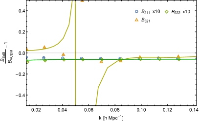
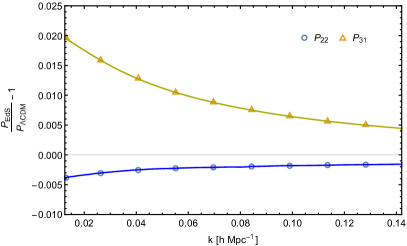
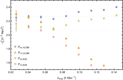
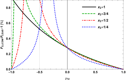
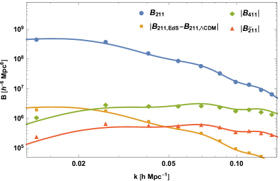
For the cosmology under consideration we have at z=0𝑧0z=0 that D2A(a)/D12(a)12.7×103subscript𝐷2𝐴𝑎superscriptsubscript𝐷12𝑎12.7superscript103{D_{2A}(a)}/{D_{1}^{2}(a)}-1\approx 2.7\times 10^{-3} and D2B(a)/D12(a)17×103subscript𝐷2𝐵𝑎superscriptsubscript𝐷12𝑎17superscript103{D_{2B}(a)}/{D_{1}^{2}(a)}-1\approx-7\times 10^{-3}. In the left panel of Fig. 3 we show the corrections to the tree-level bispectrum as a function of the cosine of the opening angle μ12=𝒌^1𝒌^2subscript𝜇12subscriptbold-^𝒌1subscriptbold-^𝒌2\mu_{12}=\bm{\hat{k}}_{1}\cdot\bm{\hat{k}}_{2} and x2=k2/k1subscript𝑥2subscript𝑘2subscript𝑘1x_{2}=k_{2}/k_{1}. In the equilateral bispectrum (x2=1,μ12=1/2formulae-sequencesubscript𝑥21subscript𝜇1212x_{2}=1,\ \mu_{12}=-1/2) this leads to a 0.5%percent0.50.5\% fractional deviation between the ΛΛ\LambdaCDM and EdS kernels, which is of the same order of magnitude as the EFT corrections we are trying to constrain here. This can be seen in the right panel of Fig. 3: the difference between the EdS and ΛΛ\LambdaCDM tree-level bispectra exceeds the amplitude of the one-loop bispectrum contribution from B411subscript𝐵411B_{411} for k<0.02hMpc1𝑘0.02superscriptMpc1k<0.02h\ \text{Mpc}^{-1} and the typical size of the EFT counterterms from B2~11subscript𝐵~211B_{\tilde{2}11} for k<0.08hMpc1𝑘0.08superscriptMpc1k<0.08h\ \text{Mpc}^{-1}. The data points show that our grid implementation of the ΛΛ\LambdaCDM second order density field agrees with the analytical calculation. We thus implemented the exact ΛΛ\LambdaCDM versions of the F2subscript𝐹2F_{2} and F3subscript𝐹3F_{3} kernels on the grid and will be using them throughout this study. The details of this implementation are discussed below in Eqs. (88) and (89). We have validated that the grid implementations of the kernels with the correct growth factors do indeed reproduce the expected deviations from the EdS approximation in the power and bispectrum, as shown in Fig. 4. In the left panel we can see that while the corrections for the B211subscript𝐵211B_{211} and B222subscript𝐵222B_{222} terms are of order 0.5%percent0.50.5\%, the corrections around the zero crossing of the combined B321subscript𝐵321B_{321} term are significant. In the right panel we reproduce the P31subscript𝑃31P_{31} and P22subscript𝑃22P_{22} corrections from Takahashi (2008) and compare them to the grid implementation, finding perfect agreement. As well will discuss below in Sec. III.1, when estimating the amplitude of the power spectrum counterterm, the 2%percent22\% corrections to P31subscript𝑃31P_{31} lead to a Δcs2=0.2h2Mpc2Δsuperscriptsubscript𝑐s20.2superscript2superscriptMpc2\Delta c_{\text{s}}^{2}=0.2h^{-2}\ \text{Mpc}^{2} change in the inferred value of of the one-loop power spectrum counterterm.

Based on results for the one-loop power spectrum Takahashi (2008); Lewandowski and Senatore (2017) in ΛΛ\LambdaCDM, and the above results, it seems plausible to expect <1%absentpercent1<1\% corrections for the one-loop bispectrum as well. This makes these corrections typically a factor of 10 smaller than the expected counterterms, such that we can ignore the ΛΛ\LambdaCDM corrections for the one-loop contributions. When pushing the accuracy to the next loop order, i.e. the two-loop bispectrum, these corrections might indeed matter.
Refer to caption
Refer to caption
Figure 3: Left panel: Fractional deviations between the ΛΛ\LambdaCDM and EdS-like quadratic coupling kernel as a function of x2=k2/k1subscript𝑥2subscript𝑘2subscript𝑘1x_{2}=k_{2}/k_{1} and μ12=𝒌^1𝒌^2subscript𝜇12subscriptbold-^𝒌1subscriptbold-^𝒌2\mu_{12}=\bm{\hat{k}}_{1}\cdot\bm{\hat{k}}_{2}. The kernels agree in the aligned configuration 𝒌1𝒌2conditionalsubscript𝒌1subscript𝒌2\bm{k}_{1}\parallel\bm{k}_{2} and show deviations of the order of 0.5%percent0.50.5\% otherwise. Right panel: Equilateral bispectrum contributions to the propagator Bn11subscript𝐵n11B_{\mathrm{n}11}. The difference between the EdS and ΛΛ\LambdaCDM tree-level bispectra (orange) exceeds the amplitude of the one-loop bispectrum contribution from B411subscript𝐵411B_{411} for k<0.02hMpc1𝑘0.02superscriptMpc1k<0.02h\ \text{Mpc}^{-1} and the typical size of the EFT counterterms from B2~11subscript𝐵~211B_{\tilde{2}11} for k<0.08hMpc1𝑘0.08superscriptMpc1k<0.08h\ \text{Mpc}^{-1}. The orange data points show that our grid implementation of the ΛΛ\LambdaCDM second order density field agrees with the analytical calculation.
Refer to caption
Refer to caption
Figure 4: Left panel: Ratio of the bispectrum contributions up to one-loop in the equilateral configuration with EdS and ΛΛ\LambdaCDM growth factors, where the relative deviation of B211subscript𝐵211B_{211} and B222subscript𝐵222B_{222} has been multiplied by ten to improve visibility. The pole is due to the sign-change of the sum of the two contributions, B321asubscript𝐵321𝑎B_{321a} and B321bsubscript𝐵321𝑏B_{321b}. Right panel: The ratio of the power spectrum contributions at one-loop with EdS and ΛΛ\LambdaCDM growth factors. Note that the change in P31subscript𝑃31P_{31} leads to a shift in the inferred cs2superscriptsubscript𝑐s2c_{\text{s}}^{2} as shown in Fig. 7.
Refer to caption
Refer to caption
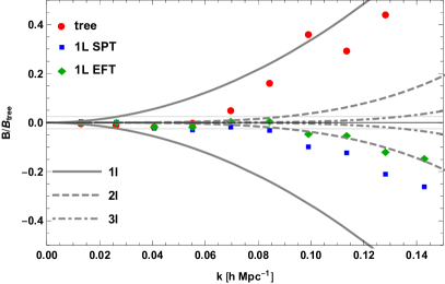
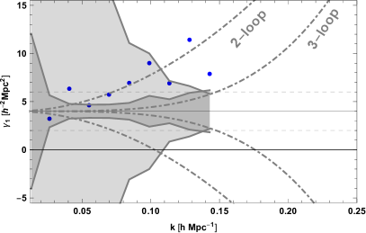
Figure 5: Left panel: Ratio of the residual bispectra and the tree-level bispectrum in the equilateral configuration. We show the difference between non-linear bispectrum and tree-level (red), one-loop SPT (blue), and one-loop EFT (green). We overplot the theoretical errors defined in Eq. (91). We see that the one-loop theoretical error (solid grey) does indeed form an appropriate envelope for the residual corrections once the tree-level prediction has been subtracted from the data. Right panel: Scale dependence of the bispectrum counterterm amplitude γ2subscript𝛾2\gamma_{2} in the equilateral configuration. We show the statistical errors without CVC (light shaded) and with CVC (dark shaded). Only with CVC can we get close to the true large scale limit before the theoretical error bars induced by two-loop terms take over.

II.5.2 UV-sensitivity

The bispectrum term B321,bsubscript𝐵321𝑏B_{321,b}, defined in Eq. (62), can be written in terms of P31subscript𝑃31P_{31} as

B321,b(𝒌1,𝒌2)=2F2(s)(𝐤1,𝐤2)P31(k1)P11(k2).subscript𝐵321𝑏subscript𝒌1subscript𝒌22superscriptsubscript𝐹2(s)subscript𝐤1subscript𝐤2subscript𝑃31subscript𝑘1subscript𝑃11subscript𝑘2B_{321,b}(\bm{k}_{1},\bm{k}_{2})=2F_{2}^{\text{(s)}}(\mathbf{k}_{1},\mathbf{k}_{2})P_{31}(k_{1})P_{11}(k_{2})\,. (73)

In analogy to Eq. (52), this leads to the UV-limit

B321,UV(𝒌1,𝒌2)=limk1,k20B321,b(𝐤1,𝐤2)=261210k12σd2F2(s)(𝐤1,𝐤2)P11(k1)P11(k2)=61210k12σd2B211(𝐤1,𝐤2),subscript𝐵321UVsubscript𝒌1subscript𝒌2subscriptsubscript𝑘1subscript𝑘20subscript𝐵321𝑏subscript𝐤1subscript𝐤2261210superscriptsubscript𝑘12superscriptsubscript𝜎d2superscriptsubscript𝐹2(s)subscript𝐤1subscript𝐤2subscript𝑃11subscript𝑘1subscript𝑃11subscript𝑘261210superscriptsubscript𝑘12superscriptsubscript𝜎d2subscript𝐵211subscript𝐤1subscript𝐤2B_{321,\text{UV}}(\bm{k}_{1},\bm{k}_{2})=\lim_{k_{1},k_{2}\to 0}B_{321,b}(\mathbf{k}_{1},\mathbf{k}_{2})=-2\frac{61}{210}k_{1}^{2}\sigma_{\text{d}}^{2}F_{2}^{\text{(s)}}(\mathbf{k}_{1},\mathbf{k}_{2})P_{11}(k_{1})P_{11}(k_{2})=-\frac{61}{210}k_{1}^{2}\sigma_{\text{d}}^{2}B_{211}(\mathbf{k}_{1},\mathbf{k}_{2})\,, (74)

based on which we can suggest the UV ansatz for the counterterm

B1~21,UV(𝒌1,𝒌2;γ1)=2γ1k12F2(𝐤1,𝐤2)P11(k1)P11(k2)=γ1k12B211(𝐤1,𝐤2),subscript𝐵~121UVsubscript𝒌1subscript𝒌2subscript𝛾12subscript𝛾1superscriptsubscript𝑘12subscript𝐹2subscript𝐤1subscript𝐤2subscript𝑃11subscript𝑘1subscript𝑃11subscript𝑘2subscript𝛾1superscriptsubscript𝑘12subscript𝐵211subscript𝐤1subscript𝐤2B_{\tilde{1}21,\mathrm{UV}}(\bm{k}_{1},\bm{k}_{2};\gamma_{1})=-2\gamma_{1}k_{1}^{2}F_{2}(\mathbf{k}_{1},\mathbf{k}_{2})P_{11}(k_{1})P_{11}(k_{2})=-\gamma_{1}k_{1}^{2}B_{211}(\mathbf{k}_{1},\mathbf{k}_{2})\,, (75)

where the fact that we are simply taking the UV-limit of F3subscript𝐹3F_{3} as we did for P31subscript𝑃31P_{31} means that we expect this γ1subscript𝛾1\gamma_{1} to be identical to cs2superscriptsubscript𝑐s2c_{\text{s}}^{2} from the power spectrum. Thus the UV inspired ansatz agrees with the full symmetry inspired counterterm, F3,UV=F~1subscript𝐹3UVsubscript~𝐹1{F}_{3,\mathrm{UV}}=\tilde{F}_{1}. The contribution from B411subscript𝐵411B_{411} has a strong UV-sensitivity that is given by the limit of the F4subscript𝐹4F_{4} kernel,

dΩ𝐪4πlimk1,k20F4(𝐤1,𝐤2,𝐪,𝐪)=118q2F4,UV(𝐤1,𝐤2),dsubscriptΩ𝐪4𝜋subscriptsubscript𝑘1subscript𝑘20subscript𝐹4subscript𝐤1subscript𝐤2𝐪𝐪118superscript𝑞2subscript𝐹4UVsubscript𝐤1subscript𝐤2\int\frac{\text{d}\Omega_{\mathbf{q}}}{4\pi}\lim_{k_{1},k_{2}\to 0}F_{4}(\mathbf{k}_{1},\mathbf{k}_{2},\mathbf{q},-\mathbf{q})=\frac{1}{18q^{2}}F_{4,\mathrm{UV}}(\mathbf{k}_{1},\mathbf{k}_{2})~{}, (76)

giving us

B411,UV(𝐤1,𝐤2)=limk1,k20B411(𝐤1,𝐤2)=2F4,UV(𝐤1,𝐤2)P(k1)P(k2)13𝐪P(q)q2=2σd2F4,UV(𝐤1,𝐤2)P(k1)P(k2),subscript𝐵411UVsubscript𝐤1subscript𝐤2subscriptsubscript𝑘1subscript𝑘20subscript𝐵411subscript𝐤1subscript𝐤22subscript𝐹4UVsubscript𝐤1subscript𝐤2𝑃subscript𝑘1𝑃subscript𝑘213subscript𝐪𝑃𝑞superscript𝑞22superscriptsubscript𝜎d2subscript𝐹4UVsubscript𝐤1subscript𝐤2𝑃subscript𝑘1𝑃subscript𝑘2\begin{split}B_{411,\text{UV}}(\mathbf{k}_{1},\mathbf{k}_{2})=\lim_{k_{1},k_{2}\to 0}B_{411}(\mathbf{k}_{1},\mathbf{k}_{2})=&2F_{4,\mathrm{UV}}(\mathbf{k}_{1},\mathbf{k}_{2})P(k_{1})P(k_{2})\frac{1}{3}\int_{\mathbf{q}}\frac{P(q)}{q^{2}}\\ =&2\sigma_{\text{d}}^{2}F_{4,\mathrm{UV}}(\mathbf{k}_{1},\mathbf{k}_{2})P(k_{1})P(k_{2})~{},\end{split} (77)

with Baldauf et al. (2015b)

F4,UV(𝒌1,𝒌2)=955218865(k12+k22)μ12261420μ12(k23k1+k13k2)12409μ123k1k256595115739μ12k1k2113190490118865(k12+k22).subscript𝐹4UVsubscript𝒌1subscript𝒌2955218865superscriptsubscript𝑘12superscriptsubscript𝑘22superscriptsubscript𝜇12261420subscript𝜇12superscriptsubscript𝑘23subscript𝑘1superscriptsubscript𝑘13subscript𝑘212409superscriptsubscript𝜇123subscript𝑘1subscript𝑘256595115739subscript𝜇12subscript𝑘1subscript𝑘2113190490118865superscriptsubscript𝑘12superscriptsubscript𝑘22\begin{split}F_{4,\mathrm{UV}}(\bm{k}_{1},\bm{k}_{2})=-\frac{9552}{18865}(k_{1}^{2}+k_{2}^{2})\mu_{12}^{2}-\frac{61}{420}\mu_{12}\left(\frac{k_{2}^{3}}{k_{1}}+\frac{k_{1}^{3}}{k_{2}}\right)\\ -\frac{12409\mu_{12}^{3}k_{1}k_{2}}{56595}-\frac{115739\mu_{12}k_{1}k_{2}}{113190}-\frac{4901}{18865}(k_{1}^{2}+k_{2}^{2})\,.\end{split} (78)

Together with Eq. (54), this suggests the UV-ansatz

B2~11,UV(𝒌1,𝒌2;γ2)=221061γ2F4,UV(𝐤1,𝐤2)P(k1)P(k2),subscript𝐵~211UVsubscript𝒌1subscript𝒌2subscript𝛾2221061subscript𝛾2subscript𝐹4UVsubscript𝐤1subscript𝐤2𝑃subscript𝑘1𝑃subscript𝑘2B_{\tilde{2}11,\text{UV}}(\bm{k}_{1},\bm{k}_{2};\gamma_{2})=2\frac{210}{61}\gamma_{2}F_{4,\mathrm{UV}}(\mathbf{k}_{1},\mathbf{k}_{2})P(k_{1})P(k_{2})~{}, (79)

which is less general than the symmetry inspired F~2subscript~𝐹2\tilde{F}_{2}.

If we were to focus entirely upon the stress-energy tensor inspired by symmetry and ignore these UV limits, we would treat γ2subscript𝛾2\gamma_{2}, ϵ1subscriptitalic-ϵ1\epsilon_{1}, ϵ2subscriptitalic-ϵ2\epsilon_{2}, and ϵ3subscriptitalic-ϵ3\epsilon_{3} in Eq. (47) as four independent parameters. Alternatively, we could fix the ratio of the parameters to match the above UV-limit of F4subscript𝐹4F_{4} and approximate F~2210/61F4,UVsubscript~𝐹221061subscript𝐹4UV\tilde{F}_{2}\approx 210/61\ F_{4,\text{UV}} by setting Baldauf et al. (2015b)

ϵ1=346614091γ2,ϵ2=728532879γ2,ϵ3=4198232879γ2.formulae-sequencesubscriptitalic-ϵ1346614091subscript𝛾2formulae-sequencesubscriptitalic-ϵ2728532879subscript𝛾2subscriptitalic-ϵ34198232879subscript𝛾2\displaystyle\epsilon_{1}=\frac{3466}{14091}\gamma_{2},\ \ \epsilon_{2}=\frac{7285}{32879}\gamma_{2},\ \ \epsilon_{3}=\frac{41982}{32879}\gamma_{2}~{}. (80)

We will consider both the UV inspired and the more general symmetry motivated counterterm parametrisations in our constraints to follow.

II.6 Estimation of Clustering Statistics

We estimate the non-linear density field by assigning particles to a regular grid using a cloud-in-cell (CIC) mass assignment scheme. The density field is subsequently transformed to Fourier space and divided by the Fourier transform of the CIC window function. The power spectrum is then estimated by averaging products of two density fields over spherical shells.

The bispectra of various combinations of fully non-linear and perturbative matter density fields are estimated using the algorithm previously employed in Baldauf et al. (2015b). We are estimating the bispectrum in linearly binned shells in k𝑘k-space using Scoccimarro et al. (1998)

B^ABC(ki,kj,kl)=VfVijl[𝐪1]i[𝐪2]j[𝐪3]lδA(𝐪1)δB(𝐪2)δC(𝐪3)(2π)3δ(D)(𝐪1+𝐪2+𝐪3),subscript^𝐵𝐴𝐵𝐶subscript𝑘𝑖subscript𝑘𝑗subscript𝑘𝑙subscript𝑉fsubscript𝑉𝑖𝑗𝑙subscriptsubscriptdelimited-[]subscript𝐪1𝑖subscriptsubscriptdelimited-[]subscript𝐪2𝑗subscriptsubscriptdelimited-[]subscript𝐪3𝑙subscript𝛿𝐴subscript𝐪1subscript𝛿𝐵subscript𝐪2subscript𝛿𝐶subscript𝐪3superscript2𝜋3superscript𝛿(D)subscript𝐪1subscript𝐪2subscript𝐪3\displaystyle\hat{B}_{ABC}(k_{i},k_{j},k_{l})=\frac{V_{\text{f}}}{V_{ijl}}\int_{[\mathbf{q}_{1}]_{i}}\int_{[\mathbf{q}_{2}]_{j}}\int_{[\mathbf{q}_{3}]_{l}}\delta_{A}(\mathbf{q}_{1})\delta_{B}(\mathbf{q}_{2})\delta_{C}(\mathbf{q}_{3})(2\pi)^{3}\delta^{\text{(D)}}(\mathbf{q}_{1}+\mathbf{q}_{2}+\mathbf{q}_{3})\,, (81)

where Vfsubscript𝑉fV_{\text{f}} is the volume of the fundamental cell Vf=(2π/L)3subscript𝑉fsuperscript2𝜋𝐿3V_{\text{f}}=(2\pi/L)^{3}. Here A, B and C stand for various combinations of fully non-linear (N𝑁N-body) and perturbative density fields on the lattice as described in the next section. The square brackets describe a linear bin (k𝑘k-space interval) around kisubscript𝑘𝑖k_{i} and

Vijl=[𝐪1]i[𝐪2]j[𝐪3]l(2π)3δ(D)(𝐪1+𝐪2+𝐪3)8π2(2π)6kikjklΔk3subscript𝑉𝑖𝑗𝑙subscriptsubscriptdelimited-[]subscript𝐪1𝑖subscriptsubscriptdelimited-[]subscript𝐪2𝑗subscriptsubscriptdelimited-[]subscript𝐪3𝑙superscript2𝜋3superscript𝛿(D)subscript𝐪1subscript𝐪2subscript𝐪38superscript𝜋2superscript2𝜋6subscript𝑘𝑖subscript𝑘𝑗subscript𝑘𝑙Δsuperscript𝑘3V_{ijl}=\int_{[\mathbf{q}_{1}]_{i}}\int_{[\mathbf{q}_{2}]_{j}}\int_{[\mathbf{q}_{3}]_{l}}(2\pi)^{3}\delta^{\text{(D)}}(\mathbf{q}_{1}+\mathbf{q}_{2}+\mathbf{q}_{3})\approx\frac{8\pi^{2}}{(2\pi)^{6}}k_{i}k_{j}k_{l}\Delta k^{3} (82)

is the volume of the corresponding Fourier-space shell.

The naive implementation of the above estimator would require a pass through all Nc3superscriptsubscript𝑁c3N_{\text{c}}^{3} cells for each of the Nc3superscriptsubscript𝑁c3N_{\text{c}}^{3} cells of the grid to ensure the triangle condition, but this quickly becomes unfeasible for small scales. We thus rewrite the Delta function in Eq. (81) as an integral over plane waves, upon which the expression factorises

B^(ki,kj,kl)=VfVijl𝒙κ=i,j,l[𝐪]κexp[i𝐪𝒙]δ(𝐪).^𝐵subscript𝑘𝑖subscript𝑘𝑗subscript𝑘𝑙subscript𝑉fsubscript𝑉𝑖𝑗𝑙subscript𝒙subscriptproduct𝜅𝑖𝑗𝑙subscriptsubscriptdelimited-[]𝐪𝜅expdelimited-[]𝑖𝐪𝒙𝛿𝐪\displaystyle\hat{B}(k_{i},k_{j},k_{l})=\frac{V_{\textit{f}}}{V_{ijl}}\int_{\bm{x}}\prod_{\kappa=i,j,l}\int_{[\mathbf{q}]_{\kappa}}\text{exp}[i\mathbf{q}\cdot\bm{x}]\delta(\mathbf{q})\,. (83)

In a first step, we select density field Fourier modes from a shell in k𝑘k-space, Fourier transform these shells to real space and sum over the product of the Fourier transforms of the three shells. The error bars of the power spectrum and bispectrum estimators are calculated from the variance over 14 realisations of the simulation box.

II.7 EFT on the Lattice

To get to the level of precision required to measure the EFT counterterms on large scales, we need to subtract the leading perturbative orders from the measurements. If perturbation theory is calculated from the loop integrals, the predictions correspond to the infinite volume limit and would require enormous simulation volumes to beat cosmic variance. We choose instead to rely on a modest simulation volume and to beat cosmic variance by evaluating the theory for the very modes used to seed the simulation realisation. This approach has previously been used to test SPT Roth and Porciani (2011); Taruya et al. (2018, 2020), but not to our knowledge been used to constrain the EFT parameters. To do so, we take advantage of the fact the the well known recursion relations Eqs. (17) and (18) for the perturbative density field and velocity dispersion can be rewritten in terms of configuration space fields 333Note that in what follows, the velocity divergence is rescaled by 1/f1𝑓-1/\mathcal{H}f, such that θ1δ1subscript𝜃1subscript𝛿1\theta_{1}\equiv\delta_{1}.

δn=m=1n11(2n+3)(n1)[(2n+1)(θmδnm𝚿θmδnm)+2(𝚿θmθnm/2𝚿θnmθm/2+Kθm,ijKθnm,ij+θmθnm/3)]subscript𝛿nsubscriptsuperscript𝑛1𝑚112𝑛3𝑛1delimited-[]2𝑛1subscript𝜃𝑚subscript𝛿n𝑚subscript𝚿subscript𝜃𝑚bold-∇subscript𝛿n𝑚2subscript𝚿subscript𝜃𝑚bold-∇subscript𝜃n𝑚2subscript𝚿subscript𝜃n𝑚bold-∇subscript𝜃𝑚2subscript𝐾subscript𝜃𝑚𝑖𝑗subscript𝐾subscript𝜃n𝑚𝑖𝑗subscript𝜃𝑚subscript𝜃n𝑚3\begin{split}\delta_{\mathrm{n}}=&\sum^{n-1}_{m=1}\frac{1}{(2n+3)(n-1)}[(2n+1)(\theta_{m}\delta_{\mathrm{n}-m}-\bm{\Psi}_{\theta_{m}}\cdot\bm{\nabla}\delta_{\mathrm{n}-m})+\\ &2(-\bm{\Psi}_{\theta_{m}}\cdot\bm{\nabla}\theta_{\mathrm{n}-m}/2-\bm{\Psi}_{\theta_{\mathrm{n}-m}}\cdot\bm{\nabla}\theta_{m}/2+K_{\theta_{m},ij}K_{\theta_{\mathrm{n}-m},ij}+\theta_{m}\theta_{\mathrm{n}-m}/3)]\end{split} (84)

and

θn=m=1n11(2n+3)(n1)[3(θmδnm𝚿θmδnm)+2n(𝚿θmθnm/2𝚿θnmθm/2+Kθm,ijKθnm,ij+θmθnm/3)].subscript𝜃nsubscriptsuperscript𝑛1𝑚112𝑛3𝑛1delimited-[]3subscript𝜃𝑚subscript𝛿n𝑚subscript𝚿subscript𝜃𝑚bold-∇subscript𝛿n𝑚2𝑛subscript𝚿subscript𝜃𝑚bold-∇subscript𝜃n𝑚2subscript𝚿subscript𝜃n𝑚bold-∇subscript𝜃𝑚2subscript𝐾subscript𝜃𝑚𝑖𝑗subscript𝐾subscript𝜃n𝑚𝑖𝑗subscript𝜃𝑚subscript𝜃n𝑚3\begin{split}\theta_{\mathrm{n}}=&\sum^{n-1}_{m=1}\frac{1}{(2n+3)(n-1)}[3(\theta_{m}\delta_{\mathrm{n}-m}-\bm{\Psi}_{\theta_{m}}\cdot\bm{\nabla}\delta_{\mathrm{n}-m})+\\ &2n(-\bm{\Psi}_{\theta_{m}}\cdot\bm{\nabla}\theta_{\mathrm{n}-m}/2-\bm{\Psi}_{\theta_{\mathrm{n}-m}}\cdot\bm{\nabla}\theta_{m}/2+K_{\theta_{m},ij}K_{\theta_{\mathrm{n}-m},ij}+\theta_{m}\theta_{\mathrm{n}-m}/3)]~{}.\end{split} (85)

The displacement fields are given by

𝚿θm(𝒌)=i𝒌k2θm(𝒌)subscript𝚿subscript𝜃𝑚𝒌𝑖𝒌superscript𝑘2subscript𝜃𝑚𝒌\bm{\Psi}_{\theta_{m}}(\bm{k})=i\frac{\bm{k}}{k^{2}}\theta_{m}(\bm{k})\, (86)

and equivalently the tidal tensor is given by

Kθm,ij(𝒌)=(kikjk213δij(K))θm(𝒌).subscript𝐾subscript𝜃𝑚𝑖𝑗𝒌subscript𝑘𝑖subscript𝑘𝑗superscript𝑘213subscriptsuperscript𝛿(K)𝑖𝑗subscript𝜃𝑚𝒌K_{\theta_{m},ij}(\bm{k})=\left(\frac{k_{i}k_{j}}{k^{2}}-\frac{1}{3}\delta^{\text{(K)}}_{ij}\right)\theta_{m}(\bm{k})\,. (87)

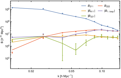
Starting from the initial Gaussian field δ1=θ1subscript𝛿1subscript𝜃1\delta_{1}=\theta_{1}, we can use these relations to generate the higher order density fields one-by-one. For numerical efficiency, spatial derivatives and inverse Laplacians are calculated in Fourier space and the fields are then transformed to configuration space where the products are evaluated. In Fig. 6 we show a comparison of analytic perturbation theory and grid calculations of the contributions to the tree-level and one-loop bispectrum. We find good agreement on all but the largest scales, where the discreteness of the simulation modes leads to minor deviations from the continuous loop calculations.

The major advantage of working with grid based perturbation theory is that it removes cosmic variance, thus acting as a cosmic variance cancellation (CVC) method. Another issue that the realisation perturbation theory helps with is the dependence of unequal time correlators on the low wavenumber or infrared modes. Equal time correlators do not suffer from this IR-sensitivity Carrasco et al. (2014b); Lewandowski and Senatore (2017). Propagators, such as correlators of the non-linear field with a number of linear fields are IR-sensitive, unequal time correlators. Since both the fully non-linear field and perturbation theory share the very infrared modes this sensitivity is accounted for in realisation perturbation theory. Evaluation of the perturbation theory loop integrals fails to account for the discrete nature of the lowest wavenumbers in the simulation box, even if a cutoff at the fundamental mode of the box is introduced.
Refer to caption
Figure 6: The realisation grid based (points) and analytic (lines) calculations of the one-loop bispectrum contributions together with their sum. As B411subscript𝐵411B_{411} and parts of B321subscript𝐵321B_{321} and B1loopsubscript𝐵1loopB_{\mathrm{1-loop}} are negative, the absolute values are shown. The error bars show the variance of the mean over the fourteen realisations. The agreement is very good with some small deviations on large scales due to the finite bin width and discrete nature of large-scale modes.

As discussed above in Sec. II.5.1 the exact ΛΛ\LambdaCDM time dependence of the SPT density field is relevant to obtain the correct counterterm amplitude on large scales. To represent the correct evolution from the simulation initial condition realisation and to cancel cosmic variance, we calculate the ΛΛ\LambdaCDM second order density field in Eq. (72) from the Gaussian initial condition δ1subscript𝛿1\delta_{1} as

δ2,ΛCDM=1721D2Aδ1δ1D12𝚿δ1δ1+27D2BKδ1,ijKδ1,ij,subscript𝛿2ΛCDM1721subscript𝐷2𝐴subscript𝛿1subscript𝛿1superscriptsubscript𝐷12subscript𝚿subscript𝛿1bold-∇subscript𝛿127subscript𝐷2𝐵subscript𝐾subscript𝛿1𝑖𝑗subscript𝐾subscript𝛿1𝑖𝑗\delta_{2,\Lambda\text{CDM}}=\frac{17}{21}D_{2A}\delta_{1}\delta_{1}-D_{1}^{2}\bm{\Psi}_{\delta_{1}}\!\cdot\!\bm{\nabla}\delta_{1}+\frac{2}{7}D_{2B}K_{\delta_{1},ij}K_{\delta_{1},ij}\,, (88)

where we used that 5/7D2A+2/7D2B=D1257subscript𝐷2𝐴27subscript𝐷2𝐵superscriptsubscript𝐷125/7D_{2A}+2/7D_{2B}=D_{1}^{2}.

Taking this to third order, we have (see App. B for the definition of the growth factors)

δ3,ΛCDM=δ1δ2[2(5D3AA,118+D3AA,26+2D3BA63)32(D3AB,19+2D3AB,29+8D3BB189)]+δ1θ2[5D3AA,118D3AA,26+52(D3AB,19+2D3AB,29+8D3BB189)2D3BA63]𝚿θ1δ2[2(5D3AA,118+D3BA21)32(D3AB,19+4D3BB63)]𝚿θ1θ2[5D3AA,118+52(D3AB,19+4D3BB63)D3BA21]𝚿δ2δ1[2(D3AA,26+D3BA21)32(2D3AB,29+4D3BB63)]𝚿θ2δ1[D3AA,26+52(2D3AB,29+4D3BB63)D3BA21]+Kδ1,ijKδ2,ij(4D3BA214D3BB21)+Kδ1,ijKθ2,ij(20D3BB632D3BA21),subscript𝛿3ΛCDMsubscript𝛿1subscript𝛿2delimited-[]25subscript𝐷3AA118subscript𝐷3AA262subscript𝐷3BA6332subscript𝐷3AB192subscript𝐷3AB298subscript𝐷3BB189subscript𝛿1subscript𝜃2delimited-[]5subscript𝐷3AA118subscript𝐷3AA2652subscript𝐷3AB192subscript𝐷3AB298subscript𝐷3BB1892subscript𝐷3BA63subscript𝚿subscript𝜃1bold-∇subscript𝛿2delimited-[]25subscript𝐷3AA118subscript𝐷3BA2132subscript𝐷3AB194subscript𝐷3BB63subscript𝚿subscript𝜃1bold-∇subscript𝜃2delimited-[]5subscript𝐷3AA11852subscript𝐷3AB194subscript𝐷3BB63subscript𝐷3BA21subscript𝚿subscript𝛿2bold-∇subscript𝛿1delimited-[]2subscript𝐷3AA26subscript𝐷3BA21322subscript𝐷3AB294subscript𝐷3BB63subscript𝚿subscript𝜃2bold-∇subscript𝛿1delimited-[]subscript𝐷3AA26522subscript𝐷3AB294subscript𝐷3BB63subscript𝐷3BA21subscript𝐾subscript𝛿1𝑖𝑗subscript𝐾subscript𝛿2𝑖𝑗4subscript𝐷3BA214subscript𝐷3BB21subscript𝐾subscript𝛿1𝑖𝑗subscript𝐾subscript𝜃2𝑖𝑗20subscript𝐷3BB632subscript𝐷3BA21\begin{split}\delta_{3,\Lambda\text{CDM}}=&\delta_{1}\delta_{2}\left[2\left(\frac{5D_{3\text{AA},1}}{18}+\frac{D_{3\text{AA},2}}{6}+\frac{2D_{3\text{BA}}}{63}\right)-\frac{3}{2}\left(\frac{D_{3\text{AB},1}}{9}+\frac{2D_{3\text{AB},2}}{9}+\frac{8D_{3\text{BB}}}{189}\right)\right]\\ &+\delta_{1}\theta_{2}\left[-\frac{5D_{3\text{AA},1}}{18}-\frac{D_{3\text{AA},2}}{6}+\frac{5}{2}\left(\frac{D_{3\text{AB},1}}{9}+\frac{2D_{3\text{AB},2}}{9}+\frac{8D_{3\text{BB}}}{189}\right)-\frac{2D_{3\text{BA}}}{63}\right]\\ &-\bm{\Psi}_{\theta_{1}}\!\cdot\!\bm{\nabla}\delta_{2}\left[2\left(\frac{5D_{3\text{AA},1}}{18}+\frac{D_{3\text{BA}}}{21}\right)-\frac{3}{2}\left(\frac{D_{3\text{AB},1}}{9}+\frac{4D_{3\text{BB}}}{63}\right)\right]\\ &-\bm{\Psi}_{\theta_{1}}\!\cdot\!\bm{\nabla}\theta_{2}\left[-\frac{5D_{3\text{AA},1}}{18}+\frac{5}{2}\left(\frac{D_{3\text{AB},1}}{9}+\frac{4D_{3\text{BB}}}{63}\right)-\frac{D_{3\text{BA}}}{21}\right]\\ &-\bm{\Psi}_{\delta_{2}}\!\cdot\!\bm{\nabla}\delta_{1}\left[2\left(\frac{D_{3\text{AA},2}}{6}+\frac{D_{3\text{BA}}}{21}\right)-\frac{3}{2}\left(\frac{2D_{3\text{AB},2}}{9}+\frac{4D_{3\text{BB}}}{63}\right)\right]\\ &-\bm{\Psi}_{\theta_{2}}\!\cdot\!\bm{\nabla}\delta_{1}\left[-\frac{D_{3\text{AA},2}}{6}+\frac{5}{2}\left(\frac{2D_{3\text{AB},2}}{9}+\frac{4D_{3\text{BB}}}{63}\right)-\frac{D_{3\text{BA}}}{21}\right]\\ &+K_{\delta_{1},ij}K_{\delta_{2},ij}\left(\frac{4D_{3\text{BA}}}{21}-\frac{4D_{3\text{BB}}}{21}\right)+K_{\delta_{1},ij}K_{\theta_{2},ij}\left(\frac{20D_{3\text{BB}}}{63}-\frac{2D_{3\text{BA}}}{21}\right)~{},\end{split} (89)

where δ2subscript𝛿2\delta_{2} and θ2subscript𝜃2\theta_{2} refer to the normal EdS second order terms. For EdS we would have D3D13subscript𝐷3superscriptsubscript𝐷13D_{3}\equiv D_{1}^{3}, leading to

δ3,EdS=7δ1δ218+25δ1θ254+2Kδ1,ijKθ2,ij97𝚿δ1δ218𝚿δ1θ29𝚿θ2δ12subscript𝛿3EdS7subscript𝛿1subscript𝛿21825subscript𝛿1subscript𝜃2542subscript𝐾subscript𝛿1𝑖𝑗subscript𝐾subscript𝜃2𝑖𝑗97subscript𝚿subscript𝛿1bold-∇subscript𝛿218subscript𝚿subscript𝛿1bold-∇subscript𝜃29subscript𝚿subscript𝜃2bold-∇subscript𝛿12\delta_{3,\text{EdS}}=\frac{7\delta_{1}\delta_{2}}{18}+\frac{25\delta_{1}\theta_{2}}{54}+\frac{2K_{\delta_{1},ij}K_{\theta_{2},ij}}{9}-\frac{7\bm{\Psi}_{\delta_{1}}\!\cdot\!\bm{\nabla}\delta_{2}}{18}-\frac{\bm{\Psi}_{\delta_{1}}\!\cdot\!\bm{\nabla}\theta_{2}}{9}-\frac{\bm{\Psi}_{\theta_{2}}\!\cdot\!\bm{\nabla}\delta_{1}}{2}~{} (90)

at z=0𝑧0z=0. We are also implementing the operators F4,UV,Γsubscript𝐹4UVΓF_{4,\mathrm{UV}},\Gamma, and Eisubscript𝐸𝑖E_{i} at the realisation level in analogy to what has been done in Abidi and Baldauf (2018) for bias parameters. We have confirmed that their clustering statistics are consistent with the analytical implementation for the counterterms. The fits to follow are, however, mostly performed with analytical implementations of the counterterms to simplify the error estimation.

II.8 Theoretical Errors

Regardless of whether we use simulations or perturbative approaches, the precision of our predictions for cosmological clustering statistics is limited. Often it is assumed that the theory works perfectly up to a certain kmaxsubscript𝑘maxk_{\text{max}} and that it cannot be trusted at all beyond that point. There are a few issues with this approach. For one, simulations have a limited precision even on the largest scales and perturbative approaches gradually lose precision as we approach the non-linear scale. It is one of the advantages of the EFTofLSS that it allows us to put an upper bound on subleading corrections, i.e. higher perturbative orders, without explicitly calculating them. This estimation of higher orders is based on the scaling of loops in scale-free universes. In a matter-only universe, there is only one scale, the non-linear scale Baldauf et al. (2016a). Thus higher loops have to scale as (k/kNL)3+nNLsuperscript𝑘subscript𝑘NL3subscript𝑛NL(k/k_{\text{NL}})^{3+n_{\text{NL}}}, where nNLsubscript𝑛NLn_{\text{NL}} is the slope at the non-linear scale. Baldauf et al. (2016a) suggested for the bispectrum error

ΔBmodel(k1,k2,k3)=3B211(k1,k2,k3)(kTkNL)(3+nNL)l,Δsubscript𝐵modelsubscript𝑘1subscript𝑘2subscript𝑘33subscript𝐵211subscript𝑘1subscript𝑘2subscript𝑘3superscriptsubscript𝑘𝑇subscript𝑘NL3subscript𝑛NL𝑙\Delta B_{\text{model}}(k_{1},k_{2},k_{3})=3B_{211}(k_{1},k_{2},k_{3})\left(\frac{k_{T}}{k_{\text{NL}}}\right)^{(3+n_{\text{NL}})l}\,, (91)

where kT=(k1+k2+k3)/3subscript𝑘Tsubscript𝑘1subscript𝑘2subscript𝑘33k_{\text{T}}=(k_{1}+k_{2}+k_{3})/3. The spectral slope of the power spectrum at the non-linear wavenumber kNL=0.3hMpc1subscript𝑘NL0.3superscriptMpc1k_{\text{NL}}=0.3h\ \text{Mpc}^{-1} is roughly nNL3/2subscript𝑛NL32n_{\text{NL}}\approx-3/2.

We show the theoretical errors in the equilateral configuration in Fig. 5. The residuals between the non-linear bispectrum and the tree-level prediction are within the bounds of the one-loop theoretical error envelope. The residual with respect to one-loop SPT is outside the two-loop envelope, but once the counterterms are included, the residuals with respect to one-loop EFT are well contained within the envelope. According to the theoretical error envelope, the two-loop terms lead to corrections of 1%percent11\% at k=0.07hMpc1𝑘0.07superscriptMpc1k=0.07h\ \text{Mpc}^{-1}, of 2%percent22\% at k=0.083hMpc1𝑘0.083superscriptMpc1k=0.083h\ \text{Mpc}^{-1} and of 5%percent55\% at k=0.11hMpc1𝑘0.11superscriptMpc1k=0.11h\ \text{Mpc}^{-1}. We will consider a 2%percent22\% error as acceptable and thus limit our fits to scales larger than kmax=0.083hMpc1subscript𝑘max0.083superscriptMpc1k_{\text{max}}=0.083h\ \text{Mpc}^{-1}.

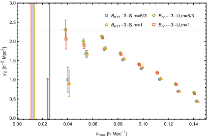
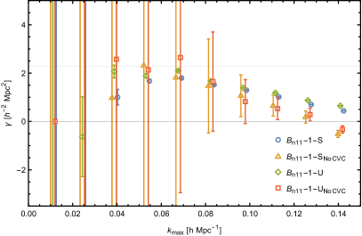
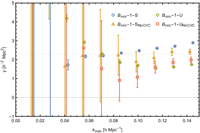
In the right panel of Fig. 5 we show the effect of higher order terms on the constraints on low-energy constants or EFT parameters. As we can see, the higher order loops start to become important even at fairly low wavenumbers, stressing the need for reducing the statistical error bars on large scales. The reduction in statistical error bars through realisation perturbation theory is demonstrated through the gray shaded regions. Only through this approach is it possible to access the regime where the one-loop counterterms asymptote to actual low-energy constants. In Baldauf et al. (2015a), a one-parameter ansatz for the two-loop power spectrum allowed to capture some of the scale dependence exhibited in the estimation of the power spectrum counterterm amplitude cs2superscriptsubscript𝑐s2c_{\text{s}}^{2}. We have some indications that a similar approach might work here but will leave its detailed discussion for future work.

III Constraining the EFT parameters

III.1 Power Spectrum

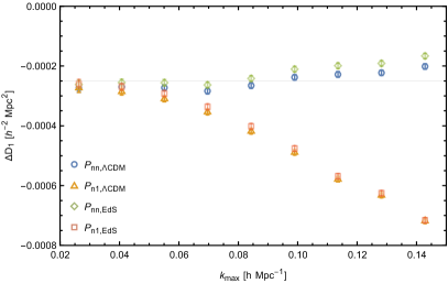
As a first step we present the inference of the power spectrum low-energy constant cs2superscriptsubscript𝑐s2c_{\text{s}}^{2} from the auto power spectrum and propagator. This measurement has been previously presented in Baldauf et al. (2015a), but their constraints were based on the EdS assumption. We are measuring the clustering statistics from a numerical simulation, which by definition has finite numerical accuracy. One of the assumptions employed in the discussion so far is that the N𝑁N-body solver correctly reproduces linear growth in the power spectrum on large scales. If the leading order growth in the simulation were off, even by a small amount, this would definitely affect our measurements of the one-loop EFT counterterms. As code comparison studies have shown Schneider et al. (2016), large-scale linear growth deviations are present due to time stepping and round off errors. To account for the possibility of the leading order linear power spectrum being slightly off, we allow for a correction term (1+2ΔD1)12Δsubscript𝐷1(1+2\Delta D_{1}) in front of the leading-order P11subscript𝑃11P_{11} contribution and fit for the free parameter (see App. C for details). The full χ2superscript𝜒2\chi^{2} for the auto power spectrum is thus given by

χnn2=k=kminkmax[Pnn(k)(1+2ΔD1)P11(k)2P31(k)2P21(k)P22(k)+2cs2k2P11(k)]2ΔPnn2(k),subscriptsuperscript𝜒2nnsuperscriptsubscript𝑘subscript𝑘minsubscript𝑘maxsuperscriptdelimited-[]subscript𝑃nn𝑘12Δsubscript𝐷1subscript𝑃11𝑘2subscript𝑃31𝑘2subscript𝑃21𝑘subscript𝑃22𝑘2superscriptsubscript𝑐s2superscript𝑘2subscript𝑃11𝑘2Δsubscriptsuperscript𝑃2nn𝑘\chi^{2}_{\mathrm{nn}}=\sum_{k=k_{\mathrm{min}}}^{k_{\mathrm{max}}}\frac{\left[P_{\mathrm{nn}}(k)-(1+2\Delta D_{1})P_{11}(k)-2P_{31}(k)-2P_{21}(k)-P_{22}(k)+2c_{\text{s}}^{2}k^{2}P_{11}(k)\right]^{2}}{\Delta P^{2}_{\mathrm{nn}}(k)}~{}, (92)

where ΔPnn2(k)Δsubscriptsuperscript𝑃2nn𝑘\Delta P^{2}_{\mathrm{nn}}(k) is the variance of the residual Pnn2P312P21P22P11subscript𝑃nn2subscript𝑃312subscript𝑃21subscript𝑃22subscript𝑃11P_{\mathrm{nn}}-2P_{31}-2P_{21}-P_{22}-P_{11}. All the terms in the above equation are evaluated using realisation perturbation theory and so share their initial conditions with the simulations. The variance of the estimator is reduced both due to the subtraction of the odd correlator P21subscript𝑃21P_{21} that would vanish in the infinite volume limit and due to the variance in the even correlators like P11subscript𝑃11P_{11} that matches the associated terms in Pnnsubscript𝑃nnP_{\mathrm{nn}}.

In the propagator we have fixed one of the linear fields, that we are cross-correlating with, thus the correction factor reduces to (1+ΔD1)1Δsubscript𝐷1(1+\Delta D_{1}). To constrain the speed-of-sound from the propagator, we minimise

χn12=k=kminkmax[Pn1(k)(1+ΔD1)P11(k)P31(k)P21(k)+cs2k2P11(k)]2ΔPn12(k),subscriptsuperscript𝜒2n1superscriptsubscript𝑘subscript𝑘minsubscript𝑘maxsuperscriptdelimited-[]subscript𝑃n1𝑘1Δsubscript𝐷1subscript𝑃11𝑘subscript𝑃31𝑘subscript𝑃21𝑘superscriptsubscript𝑐s2superscript𝑘2subscript𝑃11𝑘2Δsubscriptsuperscript𝑃2n1𝑘\chi^{2}_{\mathrm{n}1}=\sum_{k=k_{\mathrm{min}}}^{k_{\mathrm{max}}}\frac{\left[P_{\mathrm{n}1}(k)-(1+\Delta D_{1})P_{11}(k)-P_{31}(k)-P_{21}(k)+c_{\text{s}}^{2}k^{2}P_{11}(k)\right]^{2}}{\Delta P^{2}_{\mathrm{n}1}(k)}~{}, (93)

where ΔPn12(k)Δsubscriptsuperscript𝑃2n1𝑘\Delta P^{2}_{\mathrm{n}1}(k) is the variance of the residual Pn1P31P21P11subscript𝑃n1subscript𝑃31subscript𝑃21subscript𝑃11P_{\mathrm{n}1}-P_{31}-P_{21}-P_{11}. The two calculations of cs2superscriptsubscript𝑐s2c_{\text{s}}^{2} are shown in Fig. 7.

As discussed in detail in Baldauf et al. (2015a), the oscillating kmaxsubscript𝑘maxk_{\mathrm{max}} dependence seen in cs2superscriptsubscript𝑐s2c_{\text{s}}^{2} as calculated from Pnnsubscript𝑃nnP_{\mathrm{nn}} is removed when one takes into account two-loop terms which play a larger role at increasingly small physical scales (higher wavenumbers). The power spectrum and propagator constraints asymptote to the same value on large scales, roughly k<0.06hMpc1𝑘0.06superscriptMpc1k<0.06h\ \text{Mpc}^{-1}, where the one-loop approximation is sufficiently accurate. Note that without CVC, it would have been impossible to constrain the counterterm from our simulations on large scales before the loop corrections become important Baldauf et al. (2015a). In the same figure, we also show the constraints that would have been obtained if we had made the EdS approximation employed in Baldauf et al. (2015a). We see that the inferred value of cs2superscriptsubscript𝑐s2c_{\text{s}}^{2} is reduced by Δcs2=0.2h2Mpc2Δsuperscriptsubscript𝑐s20.2superscript2superscriptMpc2\Delta c_{\text{s}}^{2}=0.2h^{-2}\ \text{Mpc}^{2}. In Fig. 7, we show the counterterm amplitude corresponding to our cutoff Λ=0.3hMpc1Λ0.3superscriptMpc1\Lambda=0.3h\ \text{Mpc}^{-1}. According to Eq. (55), the extrapolation to infinite cutoff requires a subtraction of Δcs21h2Mpc2Δsuperscriptsubscript𝑐s21superscript2superscriptMpc2\Delta c_{\text{s}}^{2}\approx 1h^{-2}\ \text{Mpc}^{2}. Thus we have cs,2=1.27h2Mpc2superscriptsubscript𝑐s21.27superscript2superscriptMpc2c_{\text{s},\infty}^{2}=1.27h^{-2}\ \text{Mpc}^{2}, which is 20%percent2020\% higher than the value reported in Baldauf et al. (2015a) due to the ΛΛ\LambdaCDM corrections which were not considered in that study.

Setting the ΔD1Δsubscript𝐷1\Delta D_{1} terms to zero leads to deviations from the asymptotically flat behaviour of the estimator on large scales. We find that the ΔD1Δsubscript𝐷1\Delta D_{1} constraints themselves asymptote to 2.5×1042.5superscript104-2.5\times 10^{-4} on large scales and start to deviate past kmax=0.07hMpc1subscript𝑘max0.07superscriptMpc1k_{\text{max}}=0.07h\ \text{Mpc}^{-1} similar to the cs2superscriptsubscript𝑐s2c_{\text{s}}^{2} constraints. Note that this constraint is specific for our simulations and dependent on settings of the N𝑁N-body code.

Refer to caption
Figure 7: The speed-of-sound parameter cs2superscriptsubscript𝑐s2c_{\text{s}}^{2} as measured from both the non-linear power spectrum Pnnsubscript𝑃nnP_{\mathrm{nn}} and the propagator Pn1subscript𝑃n1P_{\mathrm{n}1}. We show constraints using the EdS approximation for perturbation theory (diamonds and squares) and using the correct ΛΛ\LambdaCDM growth factors (circles and triangles). The best fit low-energy constant is cs2=2.27h2Mpc2superscriptsubscript𝑐s22.27superscript2superscriptMpc2c_{\text{s}}^{2}=2.27h^{-2}\ \text{Mpc}^{2} (horizontal line). The difference between P31subscript𝑃31P_{31} with exact and EdS growth factors causes a Δcs20.2h2Mpc2Δsuperscriptsubscript𝑐s20.2superscript2superscriptMpc2\Delta c_{\text{s}}^{2}\approx 0.2h^{-2}\ \text{Mpc}^{2} shift to the value indicated by the horizontal dashed line. The value shown here is for cutoff Λ=0.3hMpc1Λ0.3superscriptMpc1\Lambda=0.3h\ \text{Mpc}^{-1}, and thus needs to be rescaled by Eq. (55) for comparison with values reported for ΛΛ\Lambda\to\infty.

III.2 Bispectrum

III.2.1 Fitting Procedures

We employ a number of procedures for calculating the parameters that go into the counterkernel calculations. Firstly, we decide upon a bispectrum from which to do the calculations:

  1. Bnnnsubscript𝐵nnnB_{\mathrm{n}\mathrm{n}\mathrm{n}}.

    Employing the full non-linear bispectrum, we minimise

    χnnn2(kmax)=k1,2,3=kminkmax1ΔBnnn2(k1,k2,k3)[Bnnn(k1,k2,k3)BSPTs(k1,k2,k3;ΔD1,ΔD2)B2~11s(k1,k2,k3;γ2,ϵi)B1~21s(k1,k2,k3;γ1)]2superscriptsubscript𝜒nnn2subscript𝑘maxsuperscriptsubscriptsubscript𝑘123subscript𝑘minsubscript𝑘max1Δsubscriptsuperscript𝐵2nnnsubscript𝑘1subscript𝑘2subscript𝑘3superscriptdelimited-[]subscript𝐵nnnsubscript𝑘1subscript𝑘2subscript𝑘3superscriptsubscript𝐵SPTssubscript𝑘1subscript𝑘2subscript𝑘3Δsubscript𝐷1Δsubscript𝐷2subscriptsuperscript𝐵s~211subscript𝑘1subscript𝑘2subscript𝑘3subscript𝛾2subscriptitalic-ϵ𝑖subscriptsuperscript𝐵s~121subscript𝑘1subscript𝑘2subscript𝑘3subscript𝛾12\begin{split}\chi_{\mathrm{nnn}}^{2}(k_{\mathrm{max}})&=\sum_{k_{1,2,3}=k_{\mathrm{min}}}^{k_{\mathrm{max}}}\frac{1}{\Delta B^{2}_{\mathrm{nnn}}(k_{1},k_{2},k_{3})}\Bigl{[}B_{\mathrm{nnn}}(k_{1},k_{2},k_{3})-B_{\mathrm{SPT}}^{\text{s}}(k_{1},k_{2},k_{3};\Delta D_{1},\Delta D_{2})\\ &~{}-B^{\text{s}}_{\tilde{2}11}(k_{1},k_{2},k_{3};\gamma_{2},\epsilon_{i})-B^{\text{s}}_{\tilde{1}21}(k_{1},k_{2},k_{3};\gamma_{1})\Bigr{]}^{2}~{}\end{split} (94)

    with respect to γ1subscript𝛾1\gamma_{1}, γ2subscript𝛾2\gamma_{2}, ϵ1subscriptitalic-ϵ1\epsilon_{1}, ϵ2subscriptitalic-ϵ2\epsilon_{2}, ϵ3subscriptitalic-ϵ3\epsilon_{3}, and the growth factor corrections ΔD1Δsubscript𝐷1\Delta D_{1} and ΔD2Δsubscript𝐷2\Delta D_{2}, where

    BSPTs=(1+3ΔD1)B111s+(1+2ΔD1+ΔD2)B211s+(1+2ΔD1)B311s+(1+2ΔD1)B411s+(1+ΔD1+2ΔD2)B221s+(1+ΔD1+ΔD2)B321s+(1+3ΔD2)B222s.superscriptsubscript𝐵SPTs13Δsubscript𝐷1superscriptsubscript𝐵111s12Δsubscript𝐷1Δsubscript𝐷2superscriptsubscript𝐵211s12Δsubscript𝐷1superscriptsubscript𝐵311s12Δsubscript𝐷1superscriptsubscript𝐵411s1Δsubscript𝐷12Δsubscript𝐷2superscriptsubscript𝐵221s1Δsubscript𝐷1Δsubscript𝐷2superscriptsubscript𝐵321s13Δsubscript𝐷2superscriptsubscript𝐵222s\begin{split}B_{\mathrm{SPT}}^{\text{s}}=(1+3\Delta D_{1})B_{111}^{\text{s}}+(1+2\Delta D_{1}+\Delta D_{2})B_{211}^{\text{s}}+(1+2\Delta D_{1})B_{311}^{\text{s}}+(1+2\Delta D_{1})B_{411}^{\text{s}}\\ +(1+\Delta D_{1}+2\Delta D_{2})B_{221}^{\text{s}}+(1+\Delta D_{1}+\Delta D_{2})B_{321}^{\text{s}}+(1+3\Delta D_{2})B_{222}^{\text{s}}~{}.\end{split} (95)

    The terms on the right hand side of Eq. (94) are symmetrised with respect to their external momenta.

  2. Bn11subscript𝐵n11B_{\mathrm{n}11}.

    Employing the bispectrum propagator, we minimise

    χn112(kmax)=k1,2,3=kminkmax[Bn11(k1,k2,k3)BSPT(k1,k2,k3;ΔD1,ΔD2)B2~11(k1,k2,k3;γ2,ϵi)]2ΔBn112(k1,k2,k3),superscriptsubscript𝜒n112subscript𝑘maxsuperscriptsubscriptsubscript𝑘123subscript𝑘minsubscript𝑘maxsuperscriptdelimited-[]subscript𝐵n11subscript𝑘1subscript𝑘2subscript𝑘3subscript𝐵SPTsubscript𝑘1subscript𝑘2subscript𝑘3Δsubscript𝐷1Δsubscript𝐷2subscript𝐵~211subscript𝑘1subscript𝑘2subscript𝑘3subscript𝛾2subscriptitalic-ϵ𝑖2Δsubscriptsuperscript𝐵2n11subscript𝑘1subscript𝑘2subscript𝑘3\chi_{\mathrm{n}11}^{2}(k_{\mathrm{max}})=\sum_{k_{1,2,3}=k_{\mathrm{min}}}^{k_{\mathrm{max}}}\frac{\left[B_{\mathrm{n}11}(k_{1},k_{2},k_{3})-B_{\mathrm{SPT}}(k_{1},k_{2},k_{3};\Delta D_{1},\Delta D_{2})-B_{\tilde{2}11}(k_{1},k_{2},k_{3};\gamma_{2},\epsilon_{i})\right]^{2}}{\Delta B^{2}_{\mathrm{n}11}(k_{1},k_{2},k_{3})}, (96)

    where

    BSPT=(1+ΔD1)B111+(1+ΔD2)B211+B311+B411,subscript𝐵SPT1Δsubscript𝐷1subscript𝐵1111Δsubscript𝐷2subscript𝐵211subscript𝐵311subscript𝐵411\displaystyle B_{\mathrm{SPT}}=(1+\Delta D_{1})B_{111}+(1+\Delta D_{2})B_{211}+B_{311}+B_{411}~{}, (97)

    with respect to γ2subscript𝛾2\gamma_{2}, ϵ1subscriptitalic-ϵ1\epsilon_{1}, ϵ2subscriptitalic-ϵ2\epsilon_{2}, ϵ3subscriptitalic-ϵ3\epsilon_{3}. The terms on the right hand side of Eq. (96) are not symmetrised with respect to their external momenta.

  3. Bn21subscript𝐵n21B_{\mathrm{n}21}.

    Employing our second propagator, we minimise

    χn212(kmax)=k1,2,3=kminkmax[Bn21(k1,k2,k3)BSPT(k1,k2,k3;ΔD1,ΔD2)B1~21(k1,k2,k3;γ1)]2ΔBn212(k1,k2,k3)superscriptsubscript𝜒n212subscript𝑘maxsuperscriptsubscriptsubscript𝑘123subscript𝑘minsubscript𝑘maxsuperscriptdelimited-[]subscript𝐵n21subscript𝑘1subscript𝑘2subscript𝑘3subscript𝐵SPTsubscript𝑘1subscript𝑘2subscript𝑘3Δsubscript𝐷1Δsubscript𝐷2subscript𝐵~121subscript𝑘1subscript𝑘2subscript𝑘3subscript𝛾12Δsubscriptsuperscript𝐵2n21subscript𝑘1subscript𝑘2subscript𝑘3\chi_{\mathrm{n}21}^{2}(k_{\mathrm{max}})=\sum_{k_{1,2,3}=k_{\mathrm{min}}}^{k_{\mathrm{max}}}\frac{\left[B_{\mathrm{n}21}(k_{1},k_{2},k_{3})-B_{\mathrm{SPT}}(k_{1},k_{2},k_{3};\Delta D_{1},\Delta D_{2})-B_{\tilde{1}21}(k_{1},k_{2},k_{3};\gamma_{1})\right]^{2}}{\Delta B^{2}_{\mathrm{n}21}(k_{1},k_{2},k_{3})} (98)

    with respect to γ1subscript𝛾1\gamma_{1}, where

    BSPT=(1+ΔD1)B121+(1+ΔD2)B221+B321.subscript𝐵SPT1Δsubscript𝐷1subscript𝐵1211Δsubscript𝐷2subscript𝐵221subscript𝐵321\displaystyle B_{\mathrm{SPT}}=(1+\Delta D_{1})B_{121}+(1+\Delta D_{2})B_{221}+B_{321}~{}. (99)

    The terms on the right hand side of Eq. (98) are not symmetrised with respect to their external momenta.

These functions can be differentiated with respect to the counterparameters γ1subscript𝛾1\gamma_{1}, γ2subscript𝛾2\gamma_{2}, ϵ1subscriptitalic-ϵ1\epsilon_{1}, ϵ2subscriptitalic-ϵ2\epsilon_{2}, ϵ3subscriptitalic-ϵ3\epsilon_{3} to give linear functions of said parameters. This makes constraining the parameters by finding the minima of the χ2superscript𝜒2\chi^{2} functions a simple case of solving a system of linear equations.

Ordinarily, the errors in the denominators of Equations (94), (96), and (98) would be the variance of the non-linear bispectrum and the SPT would be analytically calculated through perturbation theory. However, we propose an alternative formulation whereby the SPT components subtracted from the non-linear bispectrum come from perturbation theory on the grid and the denominator is the variance of the ensuing residual. This will reduce the overall variance of the measured parameters as it will remove the variance induced by the individual perturbative contributions to the non-linear bispectrum without affecting the measurements’ abilities to constrain the counterparameters.

In addition to choosing which non-linear bispectrum to study, we can define the following fitting procedures to constrain γ1subscript𝛾1\gamma_{1} and γ2subscript𝛾2\gamma_{2}:

  1. 1.

    Fitting for a joint EFT parameter γ𝛾\gamma after setting γ1=γ2subscript𝛾1subscript𝛾2\gamma_{1}=\gamma_{2}.

  2. 2.

    Fitting γ1=cs2subscript𝛾1superscriptsubscript𝑐s2\gamma_{1}=c_{\text{s}}^{2} from the power spectrum and using this value in the counterterm B1~21subscript𝐵~121B_{\tilde{1}21} while fitting independently for γ2subscript𝛾2\gamma_{2} in B2~11subscript𝐵~211B_{\tilde{2}11}.

  3. 3.

    Fitting for γ1subscript𝛾1\gamma_{1} and γ2subscript𝛾2\gamma_{2} independently.

  4. 4.

    Replacing the analytic counterterms with grid implementations of the counterterms B2~11,UVsubscript𝐵~211UVB_{\tilde{2}11,\text{UV}} defined in Eq. (79) and B1~21,UVsubscript𝐵~121UVB_{\tilde{1}21,\mathrm{UV}} Eq. (75) and fitting for the contained γ1subscript𝛾1\gamma_{1} and γ2subscript𝛾2\gamma_{2}.

  5. 5.

    Replacing the analytic counterterms with grid implementations of the counterterms B2~11,UVsubscript𝐵~211UVB_{\tilde{2}11,\text{UV}} defined in Eq. (79) and B1~21,UVsubscript𝐵~121UVB_{\tilde{1}21,\mathrm{UV}} Eq. (75) and fitting for a joint γ𝛾\gamma after setting γ1=γ2subscript𝛾1subscript𝛾2\gamma_{1}=\gamma_{2} .

With fittings 13131-3 for γ2subscript𝛾2\gamma_{2} we can then we can use the following parametrisations for the ϵitalic-ϵ\epsilon parameters:

  1. U.

    Inspired by UV sensitivity such that we assume F4,UV61210F~2subscript𝐹4UV61210subscript~𝐹2F_{4,\mathrm{UV}}\approx\frac{61}{210}\tilde{F}_{2}, we can use the definitions given in Equations (80) and fit B2~11subscript𝐵~211B_{\tilde{2}11} only for γ2subscript𝛾2\gamma_{2} Baldauf et al. (2015b).

  2. S.

    Inspired by symmetries, we can fit B2~11subscript𝐵~211B_{\tilde{2}11} for all four of its free parameters independently.

This provides us with a wide range of methods with which to constrain the same parameters, allowing us to cross-check the results and to compare the different procedures and comment upon their respective accuracies with reference to their assumptions. Inclusion of a free ϵ1subscriptitalic-ϵ1\epsilon_{1} parameter in Eqs. (94) and (96) results in all parameters being heavily degenerate at most values of kmaxsubscript𝑘maxk_{\mathrm{max}}, as can be quantified from the Fisher matrices of the χ2superscript𝜒2\chi^{2} functions (see App. A). For this reason, for the remainder of the analysis, the UV inspired parametrisations remain unchanged while the symmetry inspired parametrisations only minimise for γ1subscript𝛾1\gamma_{1}, γ2subscript𝛾2\gamma_{2}, ϵ2subscriptitalic-ϵ2\epsilon_{2}, and ϵ3subscriptitalic-ϵ3\epsilon_{3}, with ϵ1subscriptitalic-ϵ1\epsilon_{1} set to zero.

III.2.2 Propagator Terms

Using the propagator terms, we are able to calculate γ2subscript𝛾2\gamma_{2} and γ1subscript𝛾1\gamma_{1} in isolation and compare these results to those we obtain when studying them simultaneously in the auto bispectrum below. In the case of γ2subscript𝛾2\gamma_{2}, we did this with both the UV inspired and symmetry inspired parametrisations. Naturally, for the propagator terms we are limited to methods 3 and 4 owing to the isolated nature of the γ𝛾\gamma parameters.

Refer to caption
Refer to caption
Figure 8: Left panel: Constraints on γ2subscript𝛾2\gamma_{2} from Bn11subscript𝐵n11B_{\mathrm{n}11} with both symmetry and UV inspired parametrisations for both suggested values of the parameter m𝑚m. The differences are at the percent level; small, particularly compared to the corrections and errors we would expect from other factors such as the unmodelled contribution of the higher loop terms, but non-zero, such that for the remainder of the study of the propagator we set m=1𝑚1m=1 for the UV inspired parametrisation and m=5/3𝑚53m=5/3 for the symmetry inspired parametrisation. Note that on large scales the measurements asymptote to the power spectrum cs2superscriptsubscript𝑐s2c_{\text{s}}^{2} measurement shown by the horizontal line. Right panel: Constraints on γ2subscript𝛾2\gamma_{2} from Bn11subscript𝐵n11B_{\mathrm{n}11} with both symmetry and UV inspired parametrisations with and without cosmic variance cancellation. In the non-CVC calculations, we continued to use the residuals with subtracted grid perturbation theory and removed CVC only from the variance in the denominator of the χ2superscript𝜒2\chi^{2} to avoid issues with IR sensitivities of the propagator that are resolved by the subtraction of grid PT from the measured bispectrum propagator. The results without CVC clearly show significantly larger error bars than those without.

In Fig. 8 we compare the propagator measurements of γ1subscript𝛾1\gamma_{1} with both UV and symmetry inspired parametrisations for both suggested values of m𝑚m, as well as with both CVC and without. These show that there are small but not negligible differences between the values obtained with different values of m𝑚m and that CVC greatly reduces the error bars of the measurements. The UV inspired parametrisation replicate the UV limit of the one-loop terms when m=1𝑚1m=1 and the symmetry inspired model represents the symmetries of the EFT irrespective of m𝑚m. Given that there was a measurable difference between the constraints made with the two choices of m𝑚m, albeit a small one, we have elected to perform all future calculations in the propagator with m=1𝑚1m=1 for UV inspired fittings and m=5/3𝑚53m=5/3 for symmetry inspired fittings, and in all cases we introduce CVC.

For the growth factor corrections with the propagators, we find ΔD10.003Δsubscript𝐷10.003\Delta D_{1}\approx-0.003 and ΔD20.005Δsubscript𝐷20.005\Delta D_{2}\approx 0.005 on large scales (see App. C). The ΔD1Δsubscript𝐷1\Delta D_{1} constraint seems larger than the one obtained from the power spectrum above, but it has to be noted that it comes primarily from the noise term B111subscript𝐵111B_{111}. In App. D we validate our fitting procedure on the difference of B411subscript𝐵411B_{411} evaluated on the grid for two different cutoffs. By definition this reference field can be fit by the UV-parametrisation of B2~11subscript𝐵~211B_{\tilde{2}11}, but we also checked its ability to recover the full symmetry inspired parametrisation.

III.2.3 Auto Bispectrum

Using the full bispectrum χnnn2subscriptsuperscript𝜒2nnn\chi^{2}_{\mathrm{nnn}}, we are able to calculate γ1subscript𝛾1\gamma_{1} and γ2subscript𝛾2\gamma_{2} together, or equate them and calculate a joint γ𝛾\gamma. As we did for the propagator, we will begin by assessing the importance of CVC, the choice of the value of m𝑚m, and of our decision to use ΛΛ\LambdaCDM growth factors for δ2subscript𝛿2\delta_{2} and δ3subscript𝛿3\delta_{3} instead of the more commonly used EdS approximation. The effects of incorporating cosmic variance cancellation into the denominator of the χ2superscript𝜒2\chi^{2} for the full bispectrum are shown in the right hand panel of Fig. 9. We see that the error bars are significantly reduced in size, as they were for the propagator. As such, we use CVC in all future fittings of the auto bispectrum. In the left hand panel of the same figure we compare the Bnnnsubscript𝐵nnnB_{\mathrm{nnn}}-1 fitting for both UV and symmetry inspired parametrisations for both m=5/3𝑚53m=5/3 and m=1𝑚1m=1. While the differences between measurements with different values of m𝑚m are small, they are non-zero, and we choose to set m=1𝑚1m=1 when studying the UV inspired parametrisation and m=5/3𝑚53m=5/3 when studying the symmetry inspired parametrisations, as we did for the propagator.
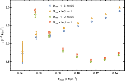
Refer to caption
Refer to caption
Figure 9: Left panel: Constraints on a joint γ𝛾\gamma from the auto bispectrum with both symmetry and UV inspired parametrisations for both suggested values of the parameter m𝑚m. As with the propagator, the differences are at the percent level. We set m=1𝑚1m=1 for the UV inspired studies of the auto bispectrum and m=5/3𝑚53m=5/3 for the symmetry inspired studies. Right panel: Constraints on the joint γ𝛾\gamma from Bnnnsubscript𝐵nnnB_{\mathrm{nnn}} with both symmetry and UV inspired parametrisations with and without cosmic variance cancellation. In the non-CVC case, we continued to use the residual with subtracted grid PT contributions and only changed the variance in the denominator, to avoid issues with IR divergences. The results without CVC clearly show larger error bars than those without.

The calculated joint γ𝛾\gamma from Bnnnsubscript𝐵nnnB_{\mathrm{nnn}}-1-S and Bnnnsubscript𝐵nnnB_{\mathrm{nnn}}-1-U are plotted in Fig. 10 with both EdS and ΛΛ\LambdaCDM growth factors for δ2subscript𝛿2\delta_{2} and δ3subscript𝛿3\delta_{3}. As can clearly be seen, the EdS results deviate quite significantly from the more accurate ΛΛ\LambdaCDM results. As such, it is clear that the use of ΛΛ\LambdaCDM growth factors is essential for high precision regularisation of the one-loop bispectrum.
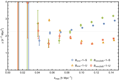
Refer to caption
Figure 10: The joint γ𝛾\gamma as calculated from the auto bispectrum using methods Bnnnsubscript𝐵nnnB_{\mathrm{nnn}}-1-S and Bnnnsubscript𝐵nnnB_{\mathrm{nnn}}-1-U with ΛΛ\LambdaCDM and EdS growth factors.

For the growth factor corrections with the auto bispectrum, we again find that ΔD10.003Δsubscript𝐷10.003\Delta D_{1}\approx-0.003 and ΔD20.005Δsubscript𝐷20.005\Delta D_{2}\approx 0.005 on large scales (see App. C). However, the corrections begin to deviate strongly from those of the propagator at k0.07hMpc1similar-to𝑘0.07superscriptMpc1k\sim 0.07h\ \text{Mpc}^{-1}.

III.2.4 Counterterm Constraints

With our growth factors, our use of CVC, and our values of the m𝑚m parameter chosen for both propagators and the auto bispectrum, we performed a number of different fittings, the calculations of γ𝛾\gamma, γ1subscript𝛾1\gamma_{1}, and γ2subscript𝛾2\gamma_{2} from which are plotted in Fig. 11. In the left hand panel we present all of the calculations of the isolated γ1subscript𝛾1\gamma_{1} and γ2subscript𝛾2\gamma_{2} from the propagator terms. The values for the various fitting procedures for γ2subscript𝛾2\gamma_{2} from Bn11subscript𝐵n11B_{\mathrm{n}11} and the Bn21subscript𝐵n21B_{\mathrm{n}21}-4 fitting for γ1subscript𝛾1\gamma_{1} all agree with one another for most values of kmaxsubscript𝑘maxk_{\mathrm{max}}, mimicking the shape of the value of cs2superscriptsubscript𝑐s2c_{\text{s}}^{2} calculated from Pn1subscript𝑃n1P_{\mathrm{n}1}, while the Bn21subscript𝐵n21B_{\mathrm{n}21}-3 calculation of γ1subscript𝛾1\gamma_{1} differs from this curve but is of roughly the same value as cs2superscriptsubscript𝑐s2c_{\text{s}}^{2} at kmax<0.07hMpc1subscript𝑘max0.07superscriptMpc1k_{\mathrm{max}}<0.07h\ \text{Mpc}^{-1}. In the right hand panel we present the fittings for γ𝛾\gamma made with the auto bispectrum. We found that while the joint γ𝛾\gamma tended to give roughly the same result for all fittings, the independent γ1subscript𝛾1\gamma_{1} and γ2subscript𝛾2\gamma_{2} sometimes gave results less in keeping with the value we would have expected by comparison with the speed of sound and were omitted from the figure. The Fisher matrix for the routine Bnnnsubscript𝐵nnnB_{\mathrm{nnn}}-3 shows γ1subscript𝛾1\gamma_{1} and γ2subscript𝛾2\gamma_{2} have a cross-correlation of 0.980.98-0.98, making them almost completely degenerate; it is possible that at higher loop order the degeneracy would be broken. As will be discussed in the next section, while the degeneracy between the two γ𝛾\gamma terms resulted in differing results for the individual counterparameters when they were allowed to vary independently, the overall counterterms still gave good fits to the residuals of the measured bispectra.
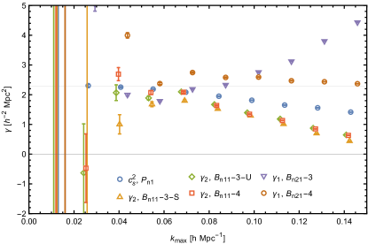
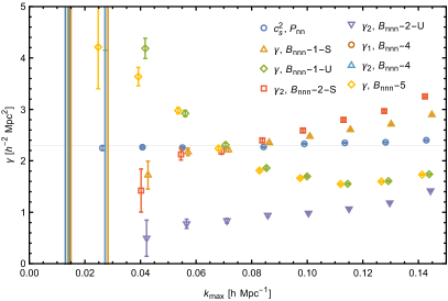
Refer to caption
Refer to caption
Figure 11: Left panel: Propagator measurements of γ1subscript𝛾1\gamma_{1} and γ2subscript𝛾2\gamma_{2} alongside the power spectrum based calculation of the speed of sound from Pn1subscript𝑃n1P_{\mathrm{n}1}. The results for γ2subscript𝛾2\gamma_{2} and the Bn21subscript𝐵n21B_{\mathrm{n21}}-4 fitting for γ1subscript𝛾1\gamma_{1} closely mimic those of cs2superscriptsubscript𝑐s2c_{\text{s}}^{2} from the power spectrum propagator while those of γ1subscript𝛾1\gamma_{1} from Bn21subscript𝐵n21B_{\mathrm{n}21}-3 follow a different curve, holding similar values to the speed of sound at k<0.1hMpc1𝑘0.1superscriptMpc1k<0.1h\ \text{Mpc}^{-1}. Right panel: Constraints on γ1subscript𝛾1\gamma_{1}, γ2subscript𝛾2\gamma_{2}, and the joint γ𝛾\gamma from the full bispectrum alongside the speed of sound constrained from Pnnsubscript𝑃nnP_{\mathrm{nn}}. The calculated values of γ1subscript𝛾1\gamma_{1} and γ2subscript𝛾2\gamma_{2} from the Bnnnsubscript𝐵nnnB_{\mathrm{nnn}}-3 procedures are omitted as the degeneracy of the two parameters made their results differ from the other fits.

As expected, the kmaxsubscript𝑘maxk_{\mathrm{max}} dependence of the results from the auto bispectrum more closely match the kmaxsubscript𝑘maxk_{\mathrm{max}} dependence of cs2superscriptsubscript𝑐s2c_{\text{s}}^{2} calculated from Pnnsubscript𝑃nnP_{\mathrm{nn}}, while those from the propagator are more similar to those of Pn1subscript𝑃n1P_{\mathrm{n}1}. On the very large scales where the cs2superscriptsubscript𝑐s2c_{\text{s}}^{2} measurements from the two power spectra agree with one another due to the small contribution from higher loop terms, we also find that our calculations from the auto and propagator bispectra begin to agree, though in both cases we begin to see results from a number of our fitting procedures that differ from those of other procedures.

In Fig. 12 we plot the inferred values of the counterterm amplitudes ϵ2subscriptitalic-ϵ2\epsilon_{2} and ϵ3subscriptitalic-ϵ3\epsilon_{3} as measured with the symmetry inspired fittings for both the auto bispectrum and the propagator. The values constrained with the symmetry-inspired ansatz have the opposite sign to those used in the UV inspired fitting.
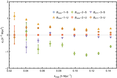
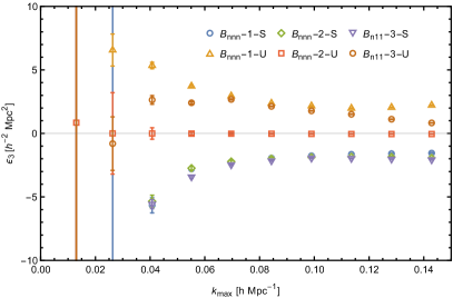
Refer to caption
Refer to caption
Figure 12: Left panel: The parameter ϵ2subscriptitalic-ϵ2\epsilon_{2} as measured from both the propagator and the auto bispectrum with the symmetry inspired parametrisation. In the case of UV inspired fits, it is simply a linear function of γ2subscript𝛾2\gamma_{2}. Right panel: The counterparameter ϵ3subscriptitalic-ϵ3\epsilon_{3} as measured from both the propagator and auto bispectrum with symmetry inspired fittings. In the case of UV inspired fits, it is a linear function of γ2subscript𝛾2\gamma_{2}. As in Fig. 11, the results from the Bnnnsubscript𝐵nnnB_{\mathrm{nnn}}-3 fitting procedures are omitted as the degeneracy of the γ𝛾\gamma terms led to results that differed strongly from those of the other fits.

The complete set of reduced χ2superscript𝜒2\chi^{2} calculations made with ΛΛ\LambdaCDM growth factors is plotted in Fig. 13. We can see that many of the fittings give good results, with a χ2superscript𝜒2\chi^{2} that crosses one roughly where we would expect given that the higher kmaxsubscript𝑘maxk_{\mathrm{max}} gives a more precise result averaging over more configurations, while the values that approach the non-linear regime begin to suffer from small scale effects that are not accounted for in our model. However, some of the fittings, most noticeably both fits made with Bn21subscript𝐵n21B_{\mathrm{n}21} and both UV inspired fits to Bn11subscript𝐵n11B_{\mathrm{n}11}, give significantly larger reduced χ2superscript𝜒2\chi^{2} values at all kmaxsubscript𝑘maxk_{\mathrm{max}} points of interest. This indicates that there is not enough freedom in the single parameter, isolated γ𝛾\gamma terms to accurately fit the data. Indeed, the χ2superscript𝜒2\chi^{2} of the UV-based ansatz is significantly larger than the χ2superscript𝜒2\chi^{2} of the symmetry-based ansatz in all cases for both the propagator and the auto bispectrum excepting Bnnnsubscript𝐵nnnB_{\mathrm{nnn}}-3, which we take as evidence that the one parameter UV inspired approximation is unable to accurately capture the bispectrum residuals.
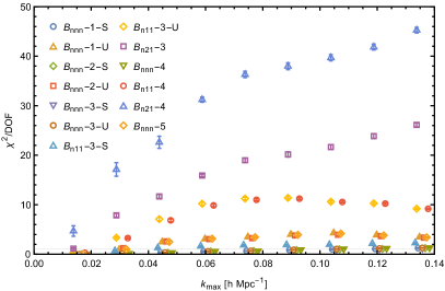
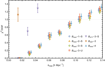
Refer to caption
Refer to caption
Figure 13: Left panel: The reduced χ2superscript𝜒2\chi^{2} for all fitting procedures of the counterterms with ΛΛ\LambdaCDM growth factors for δ2subscript𝛿2\delta_{2} and δ3subscript𝛿3\delta_{3}. Noticeably, the one-parameter fittings of isolated γ1subscript𝛾1\gamma_{1} and γ2subscript𝛾2\gamma_{2} all produce reduced χ2superscript𝜒2\chi^{2} values an order of magnitude larger than those of the multiple parameter fittings. Right panel: The same with a focus on the values close to 1. The crossing of χ2/DOF1superscript𝜒2DOF1\chi^{2}/\text{DOF}\approx 1 takes place at about kmax=0.11hMpc1subscript𝑘max0.11superscriptMpc1k_{\mathrm{max}}=0.11h\ \text{Mpc}^{-1}, which is roughly where we would expect the perturbative description of large scale structure to begin breaking down due to higher loop contributions.

The performance of the fitted models can also be assessed by comparing the value of BSPT+Bcountertermssubscript𝐵SPTsubscript𝐵countertermsB_{\mathrm{SPT}}+B_{\mathrm{counterterms}} to the measured residuals; this is shown for the equilateral configuration in Fig. 14. In the top panels of Fig. 14 we plot BnnnsB221sB311sB111ssubscriptsuperscript𝐵snnnsubscriptsuperscript𝐵s221subscriptsuperscript𝐵s311subscriptsuperscript𝐵s111B^{\mathrm{s}}_{\mathrm{nnn}}-B^{\mathrm{s}}_{221}-B^{\mathrm{s}}_{311}-B^{\mathrm{s}}_{111} against the PT calculations of B211s+B411s+B321s+B222s+B1~21s+B2~11ssubscriptsuperscript𝐵s211subscriptsuperscript𝐵s411subscriptsuperscript𝐵s321subscriptsuperscript𝐵s222subscriptsuperscript𝐵s~121subscriptsuperscript𝐵s~211B^{\mathrm{s}}_{211}+B^{\mathrm{s}}_{411}+B^{\mathrm{s}}_{321}+B^{\mathrm{s}}_{222}+B^{\mathrm{s}}_{\tilde{1}21}+B^{\mathrm{s}}_{\tilde{2}11} with counterkernels calculated according to a number of fitting procedures. The left hand panel shows the total values of these calculations while the right hand panels are normalised by the tree-level bispectra, to highlight the effects of the counterterms. Note that the parameters were constrained using the full bispectrum whereas only the equilateral configuration is shown in this figure. The central panels show the equivalent calculations for the unsymmetrised Bn11subscript𝐵n11B_{\mathrm{n}11} and the bottom panels for Bn21subscript𝐵n21B_{\mathrm{n}21}. From this figure, we can see that the results for the UV fitting procedures, 1-U, 2-U, 3-U, and 5 produce results that are at odds with the symmetry inspired procedures; method 4 is the only UV inspired fitting procedure to produce results which are in keeping with the symmetry inspired fits and closely match the residual at low k𝑘k, due to the independent fitting of γ1subscript𝛾1\gamma_{1} on a measurement of B1~21,UVsubscript𝐵~121UVB_{\tilde{1}21,\mathrm{UV}} with modes corresponding exactly to those of the residual. Together with the results discussed above with reference to Fig. 12, this could be taken to mean that the approximation B411,UVB2~11subscript𝐵411UVsubscript𝐵~211B_{411,\mathrm{UV}}\approx B_{\tilde{2}11} is not sufficient and that the counterkernel F~2subscript~𝐹2\tilde{F}_{2} must be given the full parameter freedom indicated by the symmetries of the EFT in order to accurately regularise the one-loop bispectrum. Noticeably, in the top and bottom panels of Fig. 14, which incorporate the regularisation of F~1subscript~𝐹1\tilde{F}_{1}, the limit at which regularisation becomes impossible at one-loop order is at k0.1hMpc1similar-to𝑘0.1superscriptMpc1k\sim 0.1h\ \text{Mpc}^{-1}, while in the central panels we can see that for an isolated F~2subscript~𝐹2\tilde{F}_{2} the limit is much lower, at k0.05hMpc1similar-to𝑘0.05superscriptMpc1k\sim 0.05h\ \text{Mpc}^{-1}, indicating that this estimator is much more sensitive to IR-resummation effects.
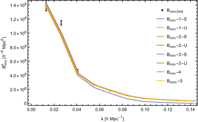
Refer to caption
Refer to caption
Refer to caption
Refer to caption
Refer to caption
Refer to caption
Figure 14: Top left panel: The measured equilateral Bnnnssuperscriptsubscript𝐵nnnsB_{\mathrm{nnn}}^{\mathrm{s}} minus the noise terms against the auto bispectrum up to one-loop calculated from perturbation theory using the values of the counterkernels taken from a variety of fitting procedures. Top right panel: The ratio Bnnns/B211ssuperscriptsubscript𝐵nnnssuperscriptsubscript𝐵211sB_{\mathrm{nnn}}^{\mathrm{s}}/B_{211}^{\mathrm{s}} for both the measured equilateral residual and the calculated equilateral bispectra with a number of fitting procedures as well as the SPT up to one-loop without counterterms. Many of the fits are good at lower momenta, where the tree-level and one-loop terms dominate, and begin to diverge from the residual at around k0.1hMpc1similar-to𝑘0.1superscriptMpc1k\sim 0.1h\ \text{Mpc}^{-1}, roughly the limit where two-loop terms would be expected to come to dominate the bispectrum. Centre left panel: The measured equilateral Bn11subscript𝐵n11B_{\mathrm{n}11} minus the noise terms against the one-loop bispectrum propagator calculated from perturbation theory using the values of the counterkernels calculated with a number of fitting procedures, together with B211subscript𝐵211B_{211}. Centre right panel: The ratio Bn11/B211subscript𝐵n11subscript𝐵211B_{\mathrm{n}11}/B_{211} for both the measured and calculated equilateral bispectra with kmax=0.084hMpc1subscript𝑘max0.084superscriptMpc1k_{\mathrm{max}}=0.084h\ \text{Mpc}^{-1} together with the SPT up to one-loop without counterterms. The fit works up until roughly this k𝑘k, at which point there becomes a noticeable deviation between the residual and the counterterms due to the increasing involvement of higher loop terms. Bottom left panel: The measured equilateral Bn21subscript𝐵n21B_{\mathrm{n}21} minus the noise terms against its one-loop perturbation theory estimator using the counterkernels calculated using methods Bn21subscript𝐵n21B_{\mathrm{n21}}-3 and Bn21subscript𝐵n21B_{\mathrm{n21}}-4, together with the SPT up to one loop without counterterms. Bottom right panel: The ratio Bn21/B211subscript𝐵n21subscript𝐵211B_{\mathrm{n}21}/B_{211} for both the measured and calculated equilateral bispectra together with the SPT up to one loop without counterterms. The fit works until k=0.1hMpc1𝑘0.1superscriptMpc1k=0.1h\ \text{Mpc}^{-1}, indicating that this is the limit at which the exclusion of two-loop terms makes accurate regularisation impossible.
Refer to caption
Refer to caption
Refer to caption
Figure 15: Top left panel: The value of F~2subscript~𝐹2\tilde{F}_{2} as a function of the ratios k2/k1subscript𝑘2subscript𝑘1k_{2}/k_{1} and k3/k2subscript𝑘3subscript𝑘2k_{3}/k_{2} with the Bnnnsubscript𝐵nnnB_{\mathrm{nnn}}-1-S parametrisation. There is a strong configuration dependence to the calculated counterterms, the sign crossing occurring in the isosceles case and becoming more prominent in the squeezed limit, that being when k30subscript𝑘30k_{3}\rightarrow 0, when k1>k2subscript𝑘1subscript𝑘2k_{1}>k_{2} and increasingly positive values in the squeezed limit as k1<k2subscript𝑘1subscript𝑘2k_{1}<k_{2}. The dark blue regions show clipping for negative values and the brown regions show clipping for positive values. Top right panel: The value of F~2subscript~𝐹2\tilde{F}_{2} as a function of the ratios k2/k1subscript𝑘2subscript𝑘1k_{2}/k_{1} and k3/k2subscript𝑘3subscript𝑘2k_{3}/k_{2} with the Bnnnsubscript𝐵nnnB_{\mathrm{nnn}}-1-U parametrisation. As before, there is a noticeable configuration dependence with the value of F~2subscript~𝐹2\tilde{F}_{2} tending towards increasingly negative values as it descends into the squeezed limit with k1>k2subscript𝑘1subscript𝑘2k_{1}>k_{2} and increasingly positive values as it descends into the same limit with k1<k2subscript𝑘1subscript𝑘2k_{1}<k_{2}. However, the configuration dependence seems to be less strong than that of the symmetry inspired fit, with a much shallower gradient visible throughout most of the plot. We can clearly see that the UV inspired fitting shows less configuration dependence than the symmetry inspired fit; this is the result of the fixing of the shape functions to be linear functions of γ𝛾\gamma, where it is important to remember that the shape functions encode the configuration dependence of the counterterm. The dark blue regions show clipping for negative values and the brown regions show clipping for positive values. Bottom panel: The fractional deviation of the above two calculations, F~2,Bnnn1S/F~2,Bnnn1U1subscript~𝐹2subscriptBnnn1Ssubscript~𝐹2subscriptBnnn1U1\tilde{F}_{2,\mathrm{B_{\mathrm{nnn}}-1-S}}/\tilde{F}_{2,\mathrm{B_{\mathrm{nnn}}-1-U}}-1. The dark blue regions show clipping for negative values and the brown regions show clipping for positive values.

Interestingly, the results from the Bnnnsubscript𝐵nnnB_{\mathrm{nnn}}-3 fitting procedure give a good fit to the simulations according to Fig. 13 and regularise the one-loop auto bispectrum approximately as well as those from the Bnnnsubscript𝐵nnnB_{\mathrm{nnn}}-1-S fitting, in spite of the differing results these procedures gave for their individual counterparameters. This indicates that the degeneracy did not affect the ability of the minimisation to give a good fit for the counterterm, merely that allowing the degenerate parameters to vary independently allowed a variety of combinations of counterparameter values to be sampled which were all still able to accurately regularise the auto bispectrum up to kmax0.1hMpc1similar-tosubscript𝑘max0.1superscriptMpc1k_{\mathrm{max}}\sim 0.1h\ \text{Mpc}^{-1}. It is notable that even the Bnnnsubscript𝐵nnnB_{\mathrm{nnn}}-3-U produced accurate results, in contrast to those of Bnnnsubscript𝐵nnnB_{\mathrm{nnn}}-1-U, indicating that allowing the γ𝛾\gamma parameters to vary separately compensated for the inaccuracy introduced by fixing the ϵisubscriptitalic-ϵ𝑖\epsilon_{i} terms.

While Fig. 14 gave us a clear test of the accuracy of the various fittings, we also wish to compare the configuration dependence of the UV and symmetry inspired parametrisations. In Fig. 15 we plot the calculated values of F~2subscript~𝐹2\tilde{F}_{2} as a function of the ratios of the momentum magnitudes k3/k1subscript𝑘3subscript𝑘1k_{3}/k_{1} and k2/k1subscript𝑘2subscript𝑘1k_{2}/k_{1} for both fitting procedures Bnnnsubscript𝐵nnnB_{\mathrm{nnn}}-1-S and Bnnnsubscript𝐵nnnB_{\mathrm{nnn}}-1-U, together with the relative deviation between the shape dependence of the two operators. As can be seen, the UV approximation shows less configuration dependence, only noticeably decreasing in the squeezed limit as k3subscript𝑘3k_{3} becomes much smaller than the other two momentum magnitudes. As well as producing a less accurate fit to the simulation residuals, the ultraviolet approximation appears to produce less shape dependence in its results, which is understandable as the approximation consists of setting the shape function parameters to be linear functions of γ2subscript𝛾2\gamma_{2}, preventing the counterterm from independently fitting to any given configuration.

IV Summary & Discussion

In this paper, we performed a precise calibration and test of the one-loop bispectrum and its counterterms in the framework of the EFTofLSS, comparing different parametrisation schemes for the counterterms. For the first time, we have considered the bispectrum propagator terms Bn11subscript𝐵n11B_{\mathrm{n}11} and Bn21subscript𝐵n21B_{\mathrm{n}21} in this context. These cross-bispectra isolate specific counterterms and allow for cross-validation of the fitting procedures and range of validity. Bn21subscript𝐵n21B_{\mathrm{n}21} contains the counterterm to B321subscript𝐵321B_{321} in isolation, which is directly related to the power spectrum counterterm for P31subscript𝑃31P_{31}. Bn11subscript𝐵n11B_{\mathrm{n}11} in turn contains the new bispectrum counterterm regularizing B411subscript𝐵411B_{411} in isolation. The full matter bispectrum contains the symmetrised version of both terms.

To uncover the counterterms on large scales, we evaluate our perturbative predictions for the very modes used to seed the simulations. This grid based realisation perturbation theory approach allows for the removal of odd correlators from measured clustering statistics and the even correlators share fluctuations with the measurements. The combination of both effects leads to a sufficient reduction on the error bars to allow for the detection of the sub-leading corrections we are after. We have confirmed that this cosmic variance cancellation significantly reduces the magnitudes of the resultant error bars for the parameter constraints. This cosmic variance cancellation enables the estimation of EFT parameters from smaller simulation volumes. The realisation perturbation theory approach would thus be uniquely suited to constrain the EFT parametrisation of baryonic physics Lewandowski et al. (2015) from numerically demanding, small-volume hydrodynamic simulations.

We have also shown that the use of the commonly used EdS approximation for the growth factors for the second order density field in the tree-level bispectrum, exceeds the one-loop corrections on large scales. We thus implemented the exact ΛΛ\LambdaCDM growth factors at quadratic and cubic order.

We found evidence for non-zero correction terms even at order k0superscript𝑘0k^{0} in the EFT. These corrections are artifacts of the numerical integration of the N𝑁N-body system, most likely round off and time stepping issues. Allowing for these bias-like terms leads to more consistent results for the actual EFT counterterms at order k2superscript𝑘2k^{2} on large scales. While the k0superscript𝑘0k^{0} terms are a nuisance parameter for our purposes, their detection on large scales can be used as a diagnostic for simulation accuracy.

The reduced χ2superscript𝜒2\chi^{2} clearly shows that the symmetry inspired models tend to provide better fits to the measurements over a wider k𝑘k-range than the UV inspired parametrisations. Yet, we find that the χ2superscript𝜒2\chi^{2} degrades past kmax=0.09hMpc1subscript𝑘max0.09superscriptMpc1k_{\text{max}}=0.09h\ \text{Mpc}^{-1}, which is in line with what was found in Baldauf et al. (2015a) for the one-loop power spectrum and also with what the theoretical errors in Sec. II.8 suggest. We find that the measurements of γ2subscript𝛾2\gamma_{2} are mostly compatible with the power spectrum value of cs,2=1.2h2Mpc2superscriptsubscript𝑐s21.2superscript2superscriptMpc2c_{\text{s},\infty}^{2}=1.2h^{-2}\ \text{Mpc}^{2}. Future work should investigate the impact of the full ΛΛ\LambdaCDM time dependence and full covariance matrix. We have considered the latter but found that our simulation suite is too small to get reliable estimates of the covariance matrix after cosmic variance cancellation. The leading non-Gaussian covariance of the bispectra without CVC could be estimated from perturbation theory on the grid Taruya et al. (2020), but after subtracting the perturbative orders, the remainder is dominated by high orders in perturbation theory and the stochastic contributions. The poor χ2superscript𝜒2\chi^{2} obtained in our fits to the propagator terms suggests that IR-resummed operators, such as those motivated by Lagrangian perturbation theory Baldauf et al. (2016b); Schmittfull et al. (2019) might be beneficial to improve the agreement between theory and simulations.

In Schmittfull et al. (2015); Abidi and Baldauf (2018) quadratic and cubic bias parameters were obtained by cross-correlating quadratic and cubic operators with the halo field. While the bias parameters start at k0superscript𝑘0k^{0} in comparison to the EFT counterterms that start at k2superscript𝑘2k^{2}, a similar approach might work to constrain EFT parameters. While this method makes estimation less complex, it buries some of the shape dependence inside the estimator. We thus preferred to extract and match the full bispectrum in the present study and leave the simplified estimator for future work.

Acknowledgements.
We would like to thank T. Nishimichi, E. Pajer, F. Schmidt, M. Simonovic, A. Taruya and M. Zaldarriaga for fruitful discussions and K. Kornet for excellent computing support. This research made use of the COSMOS supercomputer at DAMTP, Cambridge. TS acknowledges support through the Science and Technology Facilities Council Doctoral Training Centre in Data Intensive Science. TB is supported by the Stephen Hawking Advanced Fellowship at the Center for Theoretical Cosmology.

Appendix A Parameter Inference

The EFT models used in this study are linear in the parameters. In this Appendix we will briefly review the derivation of the Fisher matrix for a generic linear model before showing how it can be used to calculate the cross-correlation of any two parameters from that model and the error bars of any given parameter. We will consider a measurement 𝑩meassubscript𝑩meas\bm{B}_{\text{meas}} with a diagonal covariance matrix and variance 𝚫𝑩meas2𝚫subscriptsuperscript𝑩2meas\bm{\Delta B}^{2}_{\mathrm{meas}} and a generic theory model that is linear in the parameters such that 𝑩model=iαi𝑩model,isubscript𝑩modelsubscript𝑖subscript𝛼𝑖subscript𝑩model𝑖\bm{B}_{\mathrm{model}}=\sum_{i}\alpha_{i}\bm{B}_{\text{model},i}. Assuming Gaussian errors, we thus have

χ2=ks=kminkmax[Bmeas,siαiBmodel,i,s]2ΔBmeas,s2.superscript𝜒2superscriptsubscriptsubscript𝑘𝑠subscript𝑘minsubscript𝑘maxsuperscriptdelimited-[]subscript𝐵meas𝑠subscript𝑖subscript𝛼𝑖subscript𝐵model𝑖𝑠2Δsubscriptsuperscript𝐵2meas𝑠\chi^{2}=\sum_{k_{s}=k_{\mathrm{min}}}^{k_{\mathrm{max}}}\frac{\left[B_{\mathrm{meas},s}-\sum_{i}\alpha_{i}B_{\text{model},i,s}\right]^{2}}{\Delta B^{2}_{\mathrm{meas},s}}~{}. (100)

Taking the first derivative of Eq. (100) with respect to any given parameter αisubscript𝛼𝑖\alpha_{i} gives us

dχ2dαi=2ks=kminkmaxBmodel,i,sBmeas,sjαjBmodel,j,sΔBmeas,s2.dsuperscript𝜒2dsubscript𝛼𝑖2superscriptsubscriptsubscript𝑘𝑠subscript𝑘minsubscript𝑘maxsubscript𝐵model𝑖𝑠subscript𝐵meas𝑠subscript𝑗subscript𝛼𝑗subscript𝐵model𝑗𝑠Δsubscriptsuperscript𝐵2meas𝑠\frac{\text{d}\chi^{2}}{\text{d}\alpha_{i}}=2\sum_{k_{s}=k_{\mathrm{min}}}^{k_{\mathrm{max}}}B_{\text{model},i,s}\frac{B_{\mathrm{meas},s}-\sum_{j}\alpha_{j}B_{\text{model},j,s}}{\Delta B^{2}_{\mathrm{meas},s}}\,. (101)

Setting this first derivative to zero gives us the linear system

ks=kminkmaxBmodel,i,sBmeas,sΔBmeas,s2=jαjks=kminkmaxBmodel,i,sBmodel,j,sΔBmeas,s2.superscriptsubscriptsubscript𝑘𝑠subscript𝑘minsubscript𝑘maxsubscript𝐵model𝑖𝑠subscript𝐵meas𝑠Δsubscriptsuperscript𝐵2meas𝑠subscript𝑗subscript𝛼𝑗superscriptsubscriptsubscript𝑘𝑠subscript𝑘minsubscript𝑘maxsubscript𝐵model𝑖𝑠subscript𝐵model𝑗𝑠Δsubscriptsuperscript𝐵2meas𝑠\sum_{k_{s}=k_{\mathrm{min}}}^{k_{\mathrm{max}}}\frac{B_{\text{model},i,s}B_{\mathrm{meas},s}}{\Delta B^{2}_{\mathrm{meas},s}}=\sum_{j}\alpha_{j}\sum_{k_{s}=k_{\mathrm{min}}}^{k_{\mathrm{max}}}\frac{B_{\text{model},i,s}B_{\text{model},j,s}}{\Delta B^{2}_{\mathrm{meas},s}}\,. (102)

Taking the second derivative of which for any given parameters αisubscript𝛼𝑖\alpha_{i} and αjsubscript𝛼𝑗\alpha_{j} gives us

d2χ2dαidαj=2ks=kminkmaxBmodel,i,sBmodel,j,sΔBmeas,s2ij,superscriptd2superscript𝜒2dsubscript𝛼𝑖dsubscript𝛼𝑗2superscriptsubscriptsubscript𝑘𝑠subscript𝑘minsubscript𝑘maxsubscript𝐵model𝑖𝑠subscript𝐵model𝑗𝑠Δsubscriptsuperscript𝐵2meas𝑠subscript𝑖𝑗\frac{\text{d}^{2}\chi^{2}}{\text{d}\alpha_{i}\text{d}\alpha_{j}}=2\sum_{k_{s}=k_{\mathrm{min}}}^{k_{\mathrm{max}}}\frac{B_{\text{model},i,s}B_{\text{model},j,s}}{\Delta B^{2}_{\mathrm{meas},s}}\equiv\mathcal{F}_{ij}~{}, (103)

where \mathcal{F} is the Fisher matrix of the model in question.

We can now calculate the cross-correlation of any two parameters by looking at the ratio between the product of their isolated elements in the inverse Fisher matrix and their combined element, as given by

Cij=ij1ii1jj1.subscript𝐶𝑖𝑗superscriptsubscript𝑖𝑗1superscriptsubscript𝑖𝑖1superscriptsubscript𝑗𝑗1C_{ij}=\frac{\mathcal{F}_{ij}^{-1}}{\sqrt{\mathcal{F}_{ii}^{-1}\mathcal{F}_{jj}^{-1}}}~{}. (104)

A strong cross-correlation, that being Cij1subscript𝐶𝑖𝑗1C_{ij}\approx 1 or Cij1subscript𝐶𝑖𝑗1C_{ij}\approx-1, means that the parameters αisubscript𝛼𝑖\alpha_{i} and αjsubscript𝛼𝑗\alpha_{j} are degenerate; they correlate so strongly with one another that only one of the two is needed to determine the value of them both and allowing them both to vary freely will result in results for the individual parameters that differ markedly from those of non-degenerate parametrisations of the same functions as the model is effectively being allowed to vary one parameter in two different ways simultaneously. However, it is important to note that while degenerate parameters may give differing results for their parameters, they can still give accurate fits for the overall model.

We can also calculate the error bars for any given parameter as

σi=ii1subscript𝜎𝑖superscriptsubscript𝑖𝑖1\sigma_{i}=\sqrt{\mathcal{F}_{ii}^{-1}} (105)

and it is this definition that we use for the error bars in the figures for γ1,2subscript𝛾12\gamma_{1,2} and ϵ1,2,3subscriptitalic-ϵ123\epsilon_{1,2,3} in Sec. III.

Appendix B The Growth Factor

Here we review the ΛΛ\LambdaCDM growth factors, reproducing the work shown in Takahashi (2008).

The n𝑛n-th order growth factor Dnsubscript𝐷𝑛D_{n} describes the growth of the density perturbation δnsubscript𝛿𝑛\delta_{n} as the universe expands. It is common practice to assume EdS cosmology, such that Dn=an=1subscript𝐷𝑛superscript𝑎𝑛1D_{n}=a^{n}=1 for all D𝐷D at the present time, to simplify calculations. However, this approximation becomes increasingly inaccurate as our universe is no longer dominated by matter but by dark energy.

The linear growth factor D1subscript𝐷1D_{1} is given by the solutions to

d2dln(a2)D1a+(4+dlnHdlna)ddlnaD1a+[3+dlnHdlna32Ωm(a)]D1a=0.superscriptd2dlnsuperscript𝑎2subscript𝐷1𝑎4d𝐻d𝑎dd𝑎subscript𝐷1𝑎delimited-[]3d𝐻d𝑎32subscriptΩm𝑎subscript𝐷1𝑎0\frac{\text{d}^{2}}{\text{d}\mathrm{ln}(a^{2})}\frac{D_{1}}{a}+\left(4+\frac{\text{d}\ln H}{\text{d}\ln a}\right)\frac{\text{d}}{\text{d}\ln a}\frac{D_{1}}{a}+\left[3+\frac{\text{d}\ln H}{\text{d}\ln a}-\frac{3}{2}\Omega_{\text{m}}(a)\right]\frac{D_{1}}{a}=0~{}. (106)

with initial conditions chosen to reflect at early times the universe was approximately EdS such that at a0𝑎0a\rightarrow 0, D1(a)/a1subscript𝐷1𝑎𝑎1D_{1}(a)/a\rightarrow 1. The second order solutions are found by solving

d2dlna2D2a2+(6+dlnHdlna)ddlnaD2a2+[8+2dlnHdlna32Ωm(a)]D2a2={75[(dD1da)2+32Ωm(a)(D1a)2]forD2A,72(dD1da)2forD2B,superscriptd2dsuperscript𝑎2subscript𝐷2superscript𝑎26d𝐻d𝑎dd𝑎subscript𝐷2superscript𝑎2delimited-[]82d𝐻d𝑎32subscriptΩm𝑎subscript𝐷2superscript𝑎2cases75delimited-[]superscriptdsubscript𝐷1d𝑎232subscriptΩm𝑎superscriptsubscript𝐷1𝑎2forsubscript𝐷2𝐴72superscriptdsubscript𝐷1d𝑎2forsubscript𝐷2𝐵\begin{split}&\frac{\text{d}^{2}}{\text{d}\ln a^{2}}\frac{D_{2}}{a^{2}}+\left(6+\frac{\text{d}\ln H}{\text{d}\ln a}\right)\frac{\text{d}}{\text{d}\ln a}\frac{D_{2}}{a^{2}}+\left[8+2\frac{\text{d}\ln H}{\text{d}\ln a}-\frac{3}{2}\Omega_{\text{m}}(a)\right]\frac{D_{2}}{a^{2}}\\ &=\begin{cases}\frac{7}{5}\left[\left(\frac{\text{d}D_{1}}{\text{d}a}\right)^{2}+\frac{3}{2}\Omega_{\text{m}}(a)\left(\frac{D_{1}}{a}\right)^{2}\right]&\mathrm{for}~{}D_{2A}~{},\\ \frac{7}{2}\left(\frac{\text{d}D_{1}}{\text{d}a}\right)^{2}&\mathrm{for}~{}D_{2B}~{},\end{cases}\end{split} (107)

with initial conditions

a(t0)=0,D2A,Ba2=1,andddaD2A,Ba2=0.formulae-sequence𝑎subscript𝑡00formulae-sequencesubscript𝐷2𝐴𝐵superscript𝑎21anddd𝑎subscript𝐷2𝐴𝐵superscript𝑎20a(t_{0})=0,~{}\frac{D_{2A,B}}{a^{2}}=1,~{}\mathrm{and}~{}\frac{\text{d}}{\text{d}a}\frac{D_{2A,B}}{a^{2}}=0~{}. (108)

This gives two solutions, D2Asubscript𝐷2𝐴D_{2A} and D2Bsubscript𝐷2𝐵D_{2B}, such that

δ2(𝐤,a)=D2A(a)A(𝐤)+D2B(a)B(𝐤).subscript𝛿2𝐤𝑎subscript𝐷2𝐴𝑎𝐴𝐤subscript𝐷2𝐵𝑎𝐵𝐤\delta_{2}(\mathbf{k},a)=D_{2A}(a)A(\mathbf{k})+D_{2B}(a)B(\mathbf{k})~{}. (109)

By inserting the linear density field into Equations (10 and 11), one can derive the explicit terms for the higher order fields. The solution for the second order field is given by

A(𝐤)𝐴𝐤\displaystyle A(\mathbf{k}) =57d3𝐪α(𝐪,𝐤𝐪)δ1(𝐪)δ1(𝐤𝐪),absent57superscriptd3𝐪𝛼𝐪𝐤𝐪subscript𝛿1𝐪subscript𝛿1𝐤𝐪\displaystyle=\frac{5}{7}\int\text{d}^{3}\mathbf{q}~{}\alpha(\mathbf{q},\mathbf{k}-\mathbf{q})\delta_{1}(\mathbf{q})\delta_{1}(\mathbf{k}-\mathbf{q}), (110)
B(𝐤)𝐵𝐤\displaystyle B(\mathbf{k}) =27d3𝐪β(𝐪,𝐤𝐪)δ1(𝐪)δ1(𝐤𝐪),absent27superscriptd3𝐪𝛽𝐪𝐤𝐪subscript𝛿1𝐪subscript𝛿1𝐤𝐪\displaystyle=\frac{2}{7}\int\text{d}^{3}\mathbf{q}~{}\beta(\mathbf{q},\mathbf{k}-\mathbf{q})\delta_{1}(\mathbf{q})\delta_{1}(\mathbf{k}-\mathbf{q})~{}, (111)

The third order growth factors can be found by solving

d2dlna2D3a3+(8+dlnHdlna)ddlnaD3a3+[15+3dlnHdlna32Ωm(a)]D3a3={187[2dD1da+32Ωm(a)D1a]D2A,Ba2+187adD1daddaD2A,Ba2forD3AA,3AB,15dD1da[addaD2Aa2+2D2Aa275D1adD1da]forD3BA,92dD1da[addadD2Ba2+2D2Ba2]forD3BB,superscriptd2dsuperscript𝑎2subscript𝐷3superscript𝑎38d𝐻d𝑎dd𝑎subscript𝐷3superscript𝑎3delimited-[]153d𝐻d𝑎32subscriptΩm𝑎subscript𝐷3superscript𝑎3cases187delimited-[]2dsubscript𝐷1d𝑎32subscriptΩm𝑎subscript𝐷1𝑎subscript𝐷2𝐴𝐵superscript𝑎2187𝑎dsubscript𝐷1d𝑎dd𝑎subscript𝐷2𝐴𝐵superscript𝑎2forsubscript𝐷3𝐴𝐴3𝐴𝐵15dsubscript𝐷1d𝑎delimited-[]𝑎dd𝑎subscript𝐷2𝐴superscript𝑎22subscript𝐷2𝐴superscript𝑎275subscript𝐷1𝑎dsubscript𝐷1d𝑎forsubscript𝐷3𝐵𝐴92dsubscript𝐷1d𝑎delimited-[]𝑎dd𝑎dsubscript𝐷2𝐵superscript𝑎22subscript𝐷2𝐵superscript𝑎2forsubscript𝐷3𝐵𝐵\begin{split}&\frac{\text{d}^{2}}{\text{d}\ln a^{2}}\frac{D_{3}}{a^{3}}+\left(8+\frac{\text{d}\ln H}{\text{d}\ln a}\right)\frac{\text{d}}{\text{d}\ln a}\frac{D_{3}}{a^{3}}+\left[15+3\frac{\text{d}\ln H}{\text{d}\ln a}-\frac{3}{2}\Omega_{\text{m}}(a)\right]\frac{D_{3}}{a^{3}}\\ &=\begin{cases}\frac{18}{7}\left[2\frac{\text{d}D_{1}}{\text{d}a}+\frac{3}{2}\Omega_{\text{m}}(a)\frac{D_{1}}{a}\right]\frac{D_{2A,B}}{a^{2}}+\frac{18}{7}a\frac{\text{d}D_{1}}{\text{d}a}\frac{\text{d}}{\text{d}a}\frac{D_{2A,B}}{a^{2}}&\mathrm{for}~{}D_{3AA,3AB}~{},\\ 15\frac{\text{d}D_{1}}{\text{d}a}\left[a\frac{\text{d}}{\text{d}a}\frac{D_{2A}}{a^{2}}+2\frac{D_{2A}}{a^{2}}-\frac{7}{5}\frac{D_{1}}{a}\frac{\text{d}D_{1}}{\text{d}a}\right]&\mathrm{for}~{}D_{3BA}~{},\\ \frac{9}{2}\frac{\text{d}D_{1}}{\text{d}a}\left[a\frac{\text{d}}{\text{d}a}\frac{\text{d}D_{2B}}{a^{2}}+2\frac{D_{2B}}{a^{2}}\right]&\mathrm{for}~{}D_{3BB}~{},\end{cases}\end{split} (112)

in combination with the consistency conditions

D3AA,2=subscript𝐷3𝐴𝐴2absent\displaystyle D_{3AA,2}= 3D1323D3AB,147D3BA1621D3BB3superscriptsubscript𝐷1323subscript𝐷3𝐴𝐵147subscript𝐷3𝐵𝐴1621subscript𝐷3𝐵𝐵\displaystyle 3D_{1}^{3}-\frac{2}{3}D_{3AB,1}-\frac{4}{7}D_{3BA}-\frac{16}{21}D_{3BB} (113)
D3AB,2=subscript𝐷3𝐴𝐵2absent\displaystyle D_{3AB,2}= 94D1354D3AA,194superscriptsubscript𝐷1354subscript𝐷3𝐴𝐴1\displaystyle\frac{9}{4}D_{1}^{3}-\frac{5}{4}D_{3AA,1} (114)

with initial conditions

D3a3=1,ddaD3a3=0.formulae-sequencesubscript𝐷3superscript𝑎31dd𝑎subscript𝐷3superscript𝑎30\frac{D_{3}}{a^{3}}=1,~{}\frac{\text{d}}{\text{d}a}\frac{D_{3}}{a^{3}}=0~{}. (115)

This gives the solution

δ3(𝐤,a)=D3AA,1(a)CAA,1(𝐤)+D3AA,2(a)CAA,2(𝐤)+D3AB,1(a)CAB,1(𝐤)+D3AB,2(a)CAB,2(𝐤)+D3BA(a)CBA(𝐤)+D3BB(a)CBB(𝐤),subscript𝛿3𝐤𝑎subscript𝐷3𝐴𝐴1𝑎subscript𝐶𝐴𝐴1𝐤subscript𝐷3𝐴𝐴2𝑎subscript𝐶𝐴𝐴2𝐤subscript𝐷3𝐴𝐵1𝑎subscript𝐶𝐴𝐵1𝐤subscript𝐷3𝐴𝐵2𝑎subscript𝐶𝐴𝐵2𝐤subscript𝐷3𝐵𝐴𝑎subscript𝐶𝐵𝐴𝐤subscript𝐷3𝐵𝐵𝑎subscript𝐶𝐵𝐵𝐤\begin{split}\delta_{3}(\mathbf{k},a)=&D_{3AA,1}(a)C_{AA,1}(\mathbf{k})+D_{3AA,2}(a)C_{AA,2}(\mathbf{k})+D_{3AB,1}(a)C_{AB,1}(\mathbf{k})\\ &+D_{3AB,2}(a)C_{AB,2}(\mathbf{k})+D_{3BA}(a)C_{BA}(\mathbf{k})+D_{3BB}(a)C_{BB}(\mathbf{k})~{},\end{split} (116)

where

CAA,1(𝐤)subscript𝐶𝐴𝐴1𝐤\displaystyle C_{AA,1}(\mathbf{k}) =718d3𝐪α(𝐪,𝐤𝐪)δ1(𝐪)A(𝐤𝐪),absent718superscript𝑑3𝐪𝛼𝐪𝐤𝐪subscript𝛿1𝐪𝐴𝐤𝐪\displaystyle=\frac{7}{18}\int d^{3}\mathbf{q}~{}\alpha(\mathbf{q},\mathbf{k}-\mathbf{q})\delta_{1}(\mathbf{q})A(\mathbf{k}-\mathbf{q}), (117)
CAA,2(𝐤)subscript𝐶𝐴𝐴2𝐤\displaystyle C_{AA,2}(\mathbf{k}) =730d3𝐪α(𝐪,𝐤𝐪)δ1(𝐤𝐪)A(𝐪),absent730superscript𝑑3𝐪𝛼𝐪𝐤𝐪subscript𝛿1𝐤𝐪𝐴𝐪\displaystyle=\frac{7}{30}\int d^{3}\mathbf{q}~{}\alpha(\mathbf{q},\mathbf{k}-\mathbf{q})\delta_{1}(\mathbf{k}-\mathbf{q})A(\mathbf{q}), (118)
CAB,1(𝐤)subscript𝐶𝐴𝐵1𝐤\displaystyle C_{AB,1}(\mathbf{k}) =718d3𝐪α(𝐪,𝐤𝐪)δ1(𝐪)B(𝐤𝐪),absent718superscript𝑑3𝐪𝛼𝐪𝐤𝐪subscript𝛿1𝐪𝐵𝐤𝐪\displaystyle=\frac{7}{18}\int d^{3}\mathbf{q}~{}\alpha(\mathbf{q},\mathbf{k}-\mathbf{q})\delta_{1}(\mathbf{q})B(\mathbf{k}-\mathbf{q}), (119)
CAB,2(𝐤)subscript𝐶𝐴𝐵2𝐤\displaystyle C_{AB,2}(\mathbf{k}) =79d3𝐪α(𝐪,𝐤𝐪)δ1(𝐤𝐪)B(𝐪),absent79superscript𝑑3𝐪𝛼𝐪𝐤𝐪subscript𝛿1𝐤𝐪𝐵𝐪\displaystyle=\frac{7}{9}\int d^{3}\mathbf{q}~{}\alpha(\mathbf{q},\mathbf{k}-\mathbf{q})\delta_{1}(\mathbf{k}-\mathbf{q})B(\mathbf{q}), (120)
CBA(𝐤)subscript𝐶𝐵𝐴𝐤\displaystyle C_{BA}(\mathbf{k}) =215d3𝐪β(𝐪,𝐤𝐪)δ1(𝐪)A(𝐤𝐪),absent215superscript𝑑3𝐪𝛽𝐪𝐤𝐪subscript𝛿1𝐪𝐴𝐤𝐪\displaystyle=\frac{2}{15}\int d^{3}\mathbf{q}~{}\beta(\mathbf{q},\mathbf{k}-\mathbf{q})\delta_{1}(\mathbf{q})A(\mathbf{k}-\mathbf{q}), (121)
CBB(𝐤)subscript𝐶𝐵𝐵𝐤\displaystyle C_{BB}(\mathbf{k}) =49d3𝐪β(𝐪,𝐤𝐪)δ1(𝐤𝐪)B(𝐪),absent49superscript𝑑3𝐪𝛽𝐪𝐤𝐪subscript𝛿1𝐤𝐪𝐵𝐪\displaystyle=\frac{4}{9}\int d^{3}\mathbf{q}~{}\beta(\mathbf{q},\mathbf{k}-\mathbf{q})\delta_{1}(\mathbf{k}-\mathbf{q})B(\mathbf{q}), (122)

The differences between the EdS and ΛΛ\LambdaCDM growth factors is small, but may be large enough to cause percent scale errors in calculations. In Sec. III.2.2 and III.2.3 we compare results for the second and third order density fields with both growth factors and show that the differences can be significant for quantifying the sub-leading corrections induced by one-loop perturbation theory.

Appendix C Linear Growth Corrections

In this Appendix we briefly discuss the bias-like k0superscript𝑘0k^{0} corrections to the linear and quadratic matter density fields that we introduced to account for inaccurate growth factors in the the N𝑁N-body simulations.

The time evolution in the simulations has finite precision and can lead to sub-percent level inaccuracies in the density fields measured at z=0𝑧0z=0 (a=1𝑎1a=1). To account for these numerical errors, we introduce corrective terms into the definition of the first and second order density fields and fit for them as independent parameters of the model, giving us the following non-linear density field up to fourth order:

δn(𝒙,t)=(1+ΔD1)δ1(𝒙,t)+(1+ΔD2)δ2(𝒙,t)+δ3(𝒙,t)+δ4(𝒙,t).subscript𝛿n𝒙𝑡1Δsubscript𝐷1subscript𝛿1𝒙𝑡1Δsubscript𝐷2subscript𝛿2𝒙𝑡subscript𝛿3𝒙𝑡subscript𝛿4𝒙𝑡\delta_{\text{n}}(\bm{x},t)=(1+\Delta D_{1})\delta_{1}(\bm{x},t)+(1+\Delta D_{2})\delta_{2}(\bm{x},t)+\delta_{3}(\bm{x},t)+\delta_{4}(\bm{x},t)~{}. (123)

Beyond leading order, this parametrisation might not be the most generic ansatz, but we will leave a more detailed study of the growth systematics in simulations to future inquiry.

Fig. 16 shows the calculated value of the growth factor corrections from both the bispectra and the power spectra. Both the auto power spectrum and propagator measurements asymptote to ΔD12.5×104Δsubscript𝐷12.5superscript104\Delta D_{1}\approx-2.5\times 10^{-4} on large scales. The range over which the ΔD1Δsubscript𝐷1\Delta D_{1} measurements agree conforms with the range over which the cs2superscriptsubscript𝑐s2c_{\text{s}}^{2} measurements agree. The clear detection of this linear growth correction indicates that the linear growth in the simulations has a fractional systematic error of the same magnitude. While an offset this small might not be of any relevance for survey analysis, our ability to detect this offset proves the power of our realisation based perturbation theory approach. It can in fact be used to diagnose the accuracy of the N𝑁N-body code on large scales.

Refer to caption
Refer to caption
Refer to caption
Refer to caption
Refer to caption
Figure 16: Top left panel: The growth factor correction ΔD1Δsubscript𝐷1\Delta D_{1} from the auto bispectrum. Top right panel: The growth factor correction ΔD1Δsubscript𝐷1\Delta D_{1} from the propagators. Centre left panel: The growth factor correction ΔD2Δsubscript𝐷2\Delta D_{2} from the auto bispectrum. The results for fitting procedure Bnnnsubscript𝐵nnnB_{\mathrm{nnn}}-5 are omitted as they were significantly larger than the others. Centre right panel: The growth factor correction ΔD2Δsubscript𝐷2\Delta D_{2} from the propagators. Bottom panel: The growth factor correction ΔD1Δsubscript𝐷1\Delta D_{1} as calculated from the power spectra with both ΛΛ\LambdaCDM and EdS growth factors.

The constraints on ΔD1Δsubscript𝐷1\Delta D_{1} from the bispectrum are much less coherent, but it has to be stressed that they are dominated by an odd correlator, the noise term B111subscript𝐵111B_{111}. The constraints on ΔD2Δsubscript𝐷2\Delta D_{2} are much tighter and point towards ΔD20.005Δsubscript𝐷20.005\Delta D_{2}\approx 0.005 on large scales, with the constraints from the Bn11subscript𝐵𝑛11B_{n11} propagator being the most decisive.

Appendix D Fitting procedure validation

To validate our fitting and modelling procedure, we use the B411subscript𝐵411B_{411} measurement for two different cutoffs as a reference propagator measurement for which we know the exact values of the counterterm amplitude. By applying our fitting procedure to this artificial data set, we can check that our templates are correctly normalised and assess the expected error bars.

We generate our benchmark density field by calculating the difference between the fourth order density fields generated from linear density fields with two different wavenumber cutoffs Λ1subscriptΛ1\Lambda_{1} and Λ2subscriptΛ2\Lambda_{2}

δ4,S(k1,k2,k3;Λ1,Λ2)=δ4(k1,k2,k3;Λ1)δ4(k1,k2,k3;Λ2).subscript𝛿4Ssubscript𝑘1subscript𝑘2subscript𝑘3subscriptΛ1subscriptΛ2subscript𝛿4subscript𝑘1subscript𝑘2subscript𝑘3subscriptΛ1subscript𝛿4subscript𝑘1subscript𝑘2subscript𝑘3subscriptΛ2\delta_{4,\mathrm{S}}(k_{1},k_{2},k_{3};\Lambda_{1},\Lambda_{2})=\delta_{4}(k_{1},k_{2},k_{3};\Lambda_{1})-\delta_{4}(k_{1},k_{2},k_{3};\Lambda_{2})\,. (124)

Since we are calculating a 411 correlator, this is equivalent to calculating the difference between the respective bispectra

B411,S(k1,k2,k3;Λ1,Λ2)=B411(k1,k2,k3;Λ1)B411(k1,k2,k3;Λ2).subscript𝐵411Ssubscript𝑘1subscript𝑘2subscript𝑘3subscriptΛ1subscriptΛ2subscript𝐵411subscript𝑘1subscript𝑘2subscript𝑘3subscriptΛ1subscript𝐵411subscript𝑘1subscript𝑘2subscript𝑘3subscriptΛ2B_{411,\mathrm{S}}(k_{1},k_{2},k_{3};\Lambda_{1},\Lambda_{2})=B_{411}(k_{1},k_{2},k_{3};\Lambda_{1})-B_{411}(k_{1},k_{2},k_{3};\Lambda_{2})\,. (125)

Replacing the residual in the numerator of Eq. (96) with B411,Ssubscript𝐵411𝑆B_{411,S} gives us

χn11,test2(kmax)=k1,2,3=kminkmax[B411,S(k1,k2,k3;Λ1,Λ2)B2~11(k1,k2,k3;γ2,ϵi)]2ΔBn112(k1,k2,k3).superscriptsubscript𝜒n11test2subscript𝑘maxsuperscriptsubscriptsubscript𝑘123subscript𝑘minsubscript𝑘maxsuperscriptdelimited-[]subscript𝐵411Ssubscript𝑘1subscript𝑘2subscript𝑘3subscriptΛ1subscriptΛ2subscript𝐵~211subscript𝑘1subscript𝑘2subscript𝑘3subscript𝛾2subscriptitalic-ϵ𝑖2Δsubscriptsuperscript𝐵2n11subscript𝑘1subscript𝑘2subscript𝑘3\chi_{\mathrm{n}11\mathrm{,test}}^{2}(k_{\mathrm{max}})=\sum_{k_{1,2,3}=k_{\mathrm{min}}}^{k_{\mathrm{max}}}\frac{\left[B_{411,\mathrm{S}}(k_{1},k_{2},k_{3};\Lambda_{1},\Lambda_{2})-B_{\tilde{2}11}(k_{1},k_{2},k_{3};\gamma_{2},\epsilon_{i})\right]^{2}}{\Delta B^{2}_{\mathrm{n}11}(k_{1},k_{2},k_{3})}. (126)

There is no need for the ΔD1Δsubscript𝐷1\Delta D_{1} and ΔD2Δsubscript𝐷2\Delta D_{2} corrections in this case. From Eqs. (77) and (79) we can see that the results of the minimisation of Eq. (126) will give values of

γ261210[σd2(Λ1)σd2(Λ2)],subscript𝛾261210delimited-[]superscriptsubscript𝜎d2subscriptΛ1superscriptsubscript𝜎d2subscriptΛ2\gamma_{2}\approx\frac{61}{210}\left[\sigma_{\text{d}}^{2}(\Lambda_{1})-\sigma_{\text{d}}^{2}(\Lambda_{2})\right]~{}, (127)

with the ϵisubscriptitalic-ϵ𝑖\epsilon_{i} parameters being defined as in Eq. (80).

The comparison of this analytic calculation with the numerical minimisation can be used as a test of the counterterm implementation and of the minimisation infrastructure. A calculation with Λ1=0.3hMpc1subscriptΛ10.3superscriptMpc1\Lambda_{1}=0.3h\ \text{Mpc}^{-1} and Λ2=0.2hMpc1subscriptΛ20.2superscriptMpc1\Lambda_{2}=0.2h\ \text{Mpc}^{-1} shows that they do indeed produce the correct results of γ2subscript𝛾2\gamma_{2} at the kmaxsubscript𝑘maxk_{\mathrm{max}} values of interest.

References

  • Aghanim et al. (2018) N. Aghanim et al. (2018), arXiv:1807.06209.
  • Akrami et al. (2018) Y. Akrami et al. (2018), arXiv:1807.06205.
  • Bernardeau et al. (2002) F. Bernardeau, S. Colombi, E. Gaztanaga, and R. Scoccimarro, Phys. Rept. 367, 1 (2002), arXiv:astro-ph/0112551.
  • Baumann et al. (2012) D. Baumann, A. Nicolis, L. Senatore, and M. Zaldarriaga, JCAP 07, 051 (2012), arXiv:1004.2488.
  • Carrasco et al. (2012) J. J. M. Carrasco, M. P. Hertzberg, and L. Senatore, JHEP 09, 082 (2012), arXiv:1206.2926.
  • Carrasco et al. (2014a) J. J. M. Carrasco, S. Foreman, D. Green, and L. Senatore, JCAP 07, 057 (2014a), arXiv:1310.0464.
  • Pajer and Zaldarriaga (2013) E. Pajer and M. Zaldarriaga, JCAP 08, 037 (2013), arXiv:1301.7182.
  • Nishimichi et al. (2020) T. Nishimichi, G. D’Amico, M. M. Ivanov, L. Senatore, M. Simonović, M. Takada, M. Zaldarriaga, and P. Zhang (2020), arXiv:2003.08277.
  • Ivanov et al. (2020) M. M. Ivanov, M. Simonović, and M. Zaldarriaga, JCAP 05, 042 (2020), arXiv:1909.05277.
  • D’Amico et al. (2020) G. D’Amico, J. Gleyzes, N. Kokron, K. Markovic, L. Senatore, P. Zhang, F. Beutler, and H. Gil-Marín, JCAP 05, 005 (2020), arXiv:1909.05271.
  • Desjacques et al. (2018) V. Desjacques, D. Jeong, and F. Schmidt, Phys. Rept. 733, 1 (2018), arXiv:1611.09787.
  • Baldauf et al. (2015a) T. Baldauf, L. Mercolli, and M. Zaldarriaga, Phys. Rev. D 92, 123007 (2015a), arXiv:1507.02256.
  • Angulo et al. (2015) R. E. Angulo, S. Foreman, M. Schmittfull, and L. Senatore, JCAP 10, 039 (2015), arXiv:1406.4143.
  • Baldauf et al. (2015b) T. Baldauf, L. Mercolli, M. Mirbabayi, and E. Pajer, JCAP 05, 007 (2015b), arXiv:1406.4135.
  • Bertolini et al. (2016a) D. Bertolini, K. Schutz, M. P. Solon, J. R. Walsh, and K. M. Zurek, Phys. Rev. D 93, 123505 (2016a), arXiv:1512.07630.
  • Bertolini et al. (2016b) D. Bertolini, K. Schutz, M. P. Solon, and K. M. Zurek, JCAP 06, 052 (2016b), arXiv:1604.01770.
  • Eggemeier et al. (2019) A. Eggemeier, R. Scoccimarro, and R. E. Smith, Phys. Rev. D 99, 123514 (2019), arXiv:1812.03208.
  • Lazanu et al. (2016) A. Lazanu, T. Giannantonio, M. Schmittfull, and E. Shellard, Phys. Rev. D 93, 083517 (2016), arXiv:1510.04075.
  • Lazanu and Liguori (2018) A. Lazanu and M. Liguori, JCAP 04, 055 (2018), arXiv:1803.03184.
  • Crocce et al. (2006) M. Crocce, S. Pueblas, and R. Scoccimarro, MNRAS 373, 369 (2006), arXiv:astro-ph/0606505.
  • Springel (2005) V. Springel, MNRAS 364, 1105 (2005), arXiv:astro-ph/0505010.
  • Roth and Porciani (2011) N. Roth and C. Porciani, MNRAS 415, 829 (2011), arXiv:1101.1520.
  • Taruya et al. (2018) A. Taruya, T. Nishimichi, and D. Jeong, Phys. Rev. D 98, 103532 (2018), arXiv:1807.04215.
  • Taruya et al. (2020) A. Taruya, T. Nishimichi, and D. Jeong (2020), arXiv:2007.05504.
  • Mercolli and Pajer (2014) L. Mercolli and E. Pajer, JCAP 03, 006 (2014), arXiv:1307.3220.
  • Baldauf et al. (2016a) T. Baldauf, M. Mirbabayi, M. Simonović, and M. Zaldarriaga (2016a), arXiv:1602.00674.
  • Takahashi (2008) R. Takahashi, Prog. Theor. Phys. 120, 549 (2008), arXiv:0806.1437.
  • Fasiello and Vlah (2016) M. Fasiello and Z. Vlah, Phys. Rev. D 94, 063516 (2016), arXiv:1604.04612.
  • Lewandowski and Senatore (2017) M. Lewandowski and L. Senatore, JCAP 08, 037 (2017), arXiv:1701.07012.
  • Scoccimarro et al. (1998) R. Scoccimarro, S. Colombi, J. N. Fry, J. A. Frieman, E. Hivon, and A. Melott, ApJ 496, 586 (1998), arXiv:astro-ph/9704075.
  • Carrasco et al. (2014b) J. J. M. Carrasco, S. Foreman, D. Green, and L. Senatore, JCAP 07, 056 (2014b), arXiv:1304.4946.
  • Abidi and Baldauf (2018) M. M. Abidi and T. Baldauf, JCAP 07, 029 (2018), arXiv:1802.07622.
  • Schneider et al. (2016) A. Schneider, R. Teyssier, D. Potter, J. Stadel, J. Onions, D. S. Reed, R. E. Smith, V. Springel, F. R. Pearce, and R. Scoccimarro, JCAP 04, 047 (2016), arXiv:1503.05920.
  • Lewandowski et al. (2015) M. Lewandowski, A. Perko, and L. Senatore, JCAP 05, 019 (2015), arXiv:1412.5049.
  • Baldauf et al. (2016b) T. Baldauf, E. Schaan, and M. Zaldarriaga, JCAP 03, 017 (2016b), arXiv:1505.07098.
  • Schmittfull et al. (2019) M. Schmittfull, M. Simonović, V. Assassi, and M. Zaldarriaga, Phys. Rev. D 100, 043514 (2019), arXiv:1811.10640.
  • Schmittfull et al. (2015) M. Schmittfull, T. Baldauf, and U. Seljak, Phys. Rev. D 91, 043530 (2015), arXiv:1411.6595.