Abstract
We discuss the determination of the parton substructure of hadrons by casting it as a peculiar form of pattern recognition problem in which the pattern is a probability distribution, and we present the way this problem has been tackled and solved. Specifically, we review the NNPDF approach to PDF determination, which is based on the combination of a Monte Carlo approach with neural networks as basic underlying interpolators. We discuss the current NNPDF methodology, based on genetic minimization, and its validation through closure testing. We then present recent developments in which a hyperoptimized deep-learning framework for PDF determination is being developed, optimized, and tested.
Chapter 0 Parton distribution functions
Sumbitted for review.
To appear in the volume
Artificial Intelligence for Particle Physics, World Scientific Publishing.
TIF-UNIMI-2020-23
1 Introduction
The determination of the parton substructure of the nucleon is essentially a pattern recognition problem: given an unknown underlying function that maps input instances to actually realized outcomes, use a set of data to infer the function itself. However, the determination of parton distributions (PDFs, henceforth) determination differs from standard pattern recognition problems (such as, say, face detection) in many peculiar and perhaps unique relevant aspects. Also, whereas the first PDF determinations have been performed around forty-five years ago [1, 2, 3, 4, 5, 6] it was only recognized less than twenty years ago [7, 8, 9, 10, 11] that AI techniques could be used for PDF determination 1).
In this section we will first briefly review what the problem of PDF determination consists of, in which sense it can be viewed as a pattern recognition problem, and the peculiarities that characterize it. We will then briefly summarize the NNPDF approach to PDF determination, which is the only approach in which the problem has been tackled using AI techniques.
In Section 2 we will provide a more detailed discussion of the NNPDF tool-set used for the determination of current published PDF sets i.e. up to NNPDF3.1 [12]. We will specifically discuss the use of neural nets as PDF interpolants, PDF training using genetic minimization and cross-validation, and the validation methodology based on closure testing. In Section 3 we will then turn to a methodology that is currently being developed for future PDF determinations, which updates the standard AI tools used by NNPDF to more recent machine learning methods, relying on deterministic minimization, model optimization (hyper-optimization) and more powerful and detailed validation techniques.
1 PDF determination as an AI problem
PDFs encode the structure of strongly-interacting particles or nuclei, as probed in high-energy collisions. A review of the underlying theory is beyond the scope of this work, and the reader is referred to standard textbooks [13], summer school lecture notes [14] and recent specialized reviews [15, 16] for more detailed discussions. Here it will suffice to say that a generic observable, such as the total cross section for a “hard” (i.e., perturbatively computable in QCD) physical process in a collision between two hadrons (such as two protons at the LHC) has the structure
| (1) |
Here is the (square) center-of-mass energy of the collision (so at the LHC) and is the mass of the final state (so for Higgs production); is the measurable cross section, observed in proton-proton interactions (hadronic cross section, henceforth), while is the computable cross section, determined in perturbation theory from the interaction of two incoming partons, i.e. quarks and gluons and (partonic cross section, henceforth).
In Eq. (1) , are the PDFs: they provide information on the probability of extracting a parton of kind , (up quark, up antiquark, etc.) from incoming hadrons , . Note that PDFs are not quite probability densities, first because they are not functions but rather distributions (like the Dirac delta), and also, they are not positive definite. The PDFs are a universal property of the given hadron: e.g., the proton PDFs are the same for any process with a proton in the initial state. They depend on , which can be viewed as the fraction of the momentum of the incoming hadron carried by the given parton, so , and on the scale . The dependence on is computable in perturbation theory, just like the partonic cross section , and it is given as a set of integro-differential equations, having as initial conditions the set of PDFs at some reference scale .
The dependence of the PDFs on would be computable if one was able to solve QCD in the nonperturbative domain: i.e., if it was possible to compute the proton wave function from first principles. This is of course not the case, other than through lattice simulations [17]. Hence, in principle, PDFs for any given hadron at some reference scale are a set of well-defined functions of , namely , which depend on the single free parameter of the theory, the strong coupling (and, for heavy quark PDFs, the heavy quark masses). We know that these functions exist, but we do not know what they are: at present, they can only be determined by comparing cross sections of the form Eq. (1) for a wide enough set of observables for which the hadronic cross section is measured with sufficient precision, and the partonic cross section is known with sufficient accuracy (i.e. to high enough perturbative order in QCD, including electroweak corrections, etc.).
The traditional way the problem has been approached is by postulating a particular functional form for the dependence of the PDFs at a reference scale , given in terms of a set of free parameters; determining the PDFs at all other scales by solving perturbative evolution equations; and determining the free parameters by fitting to the data. The standard choice, adopted since the very first attempts [1] is
| (2) |
where now collectively indicates the type of parton and of parent hadron. This functional form is suggested by theory arguments (or perhaps prejudice) implying that PDFs should display power-like behavior as and as (see e.g. Ref. [18]). Note that, even if this were true, there is no reason to believe that this behavior should hold for all , and thus, given that only a finite range in is experimentally accessible (currently roughly ), it is unclear that this functional form should apply at all in the observable region. Furthermore, from the equations which govern the dependence of the PDFs, it is easy to see that even if the PDF takes the form of Eq. (2) at some scale, this form is not preserved as the scale is varied: specifically, it is corrected by terms as , and by terms as .
The fact that the simple functional form Eq. (2) is too restrictive has been rapidly recognized, and more and more elaborate functional forms have been adopted in more recent PDF determinations. For example, the gluon PDF of the proton was parametrized in the CTEQ5 [19] PDF set as
| (3) |
and in the CT18 PDF set [20] as
| (4) |
Issues related to postulating a fixed functional form for PDFs were made apparent when a determination of the uncertainties on the PDFs was first attempted [21, 22, 23]. Namely, uncertainties on the fit parameters determined by least-squares and standard error propagation turned out to be smaller by about one order of magnitude than one might reasonably expect by looking at the fluctuation of best-fit values as the underlying dataset was varied. This led to the peculiar concept of “tolerance”, namely, an a-posteriori rescaling factor of uncertainties. It is debatable how much of the need for such a rescaling is related to the bias introduced by the choice of a particular functional form. However, a not uncommon occurrence is that addition of new data, leading to a more extended parametrization (such as Eq. (1) in comparison to Eq. (3)) would lead to an increase in uncertainties. This suggests that the more restrictive parametrization might well be biased.
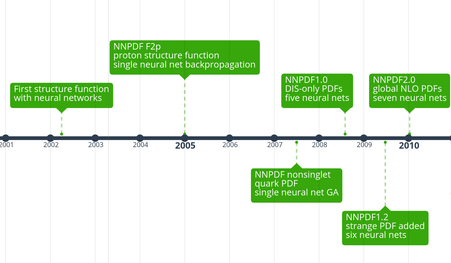
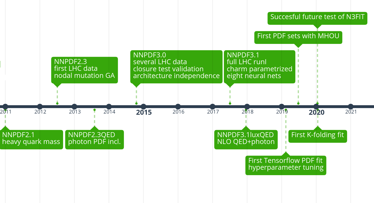
In 2002 it was first suggested [7] that these difficulties may be overcome by addressing the problem of PDF determination by means of a standard AI tool, neural networks. The basic underlying intuition is that neural networks provide a universal interpolating function, and that by choosing a sufficiently redundant architecture any functional form can be accommodated in a bias-free way, while avoiding overtraining through suitable training methods, as we will discuss in Sections 2, 4 below. This first suggestion was gradually developed into a systematic methodology for PDF determination through a series of intermediate steps (see Figure 1) involving, on the methodological side, a number of subsequent improvements, to be discussed below, and a set of validation and testing techniques. The more recent successors NNPDF3.0 [24] and NNPDF3.1 [12] of the first PDF set developed using this methodology (NNPDF1.0 [10]) are currently the most widely cited PDF sets.
It should now be clear in which sense PDF determination can be viewed as a pattern recognition problem, and what are its peculiar features. As in standard pattern recognition, the main goal is to determine a set of unknown underlying functions from data instances, with almost no knowledge of their functional form (other than loose constraints of integrability with an appropriate measure, smoothness, etc.). Unlike in the simplest pattern recognition problems, the functions provide continuous output (i.e. the features to be recognized are continuous), and data are not directly instances of the functions to be determined. Hence, one cannot associate an input-output pair to an individual data point. Rather, as apparent from Eq. (1), each datapoint provides an output which depends in a nonlinear way on the full set of functions evaluated at all input values, which are integrated over from some minimum (depending on the particular observable and the values of and ). This is of course common to more complex pattern recognition problems, such as in computer vision.
There are however two peculiarities in PDF determination which set it apart from most or perhaps all other applications of AI. The first is that the quantities which one is trying to determine, the PDFs, are probability distributions of observables, rather than being observables themselves. This follows from the fact that, due to the quantum nature of fundamental interactions, individual events (i.e. measurement outcomes) are stochastic, not deterministic. Even if the PDF were known exactly to absolute accuracy, the cross section would just express the probability of the observation of an event, to be determined through repeated measurements. The PDFs are accordingly probability distributions. The goal of PDF determination is to determine the probability distribution of PDFs: hence, in PDF determination one determines a probability distributions of probability distributions, i.e. a probability functional.
The second peculiarity is that in order for a PDF determination to be useful as an input to physics predictions, full knowledge of PDF correlations is needed. In fact, PDF uncertainties are typically a dominant source of uncertainty in predictions for current and future high-energy experiments [25]. But the uncertainty on each particular PDF at a given value, is correlated to the uncertainty on any other PDF at a different value , and this correlation must be accounted for in order to reliably estimate PDF uncertainties [26]. Hence, PDF determination also requires the determination a covariance matrix of uncertainties in the space of probability distributions: namely, a covariance matrix functional.
The NNPDF approach to PDF determination tackles this problem using AI tools, as we discuss in the next section.
2 The NNPDF approach
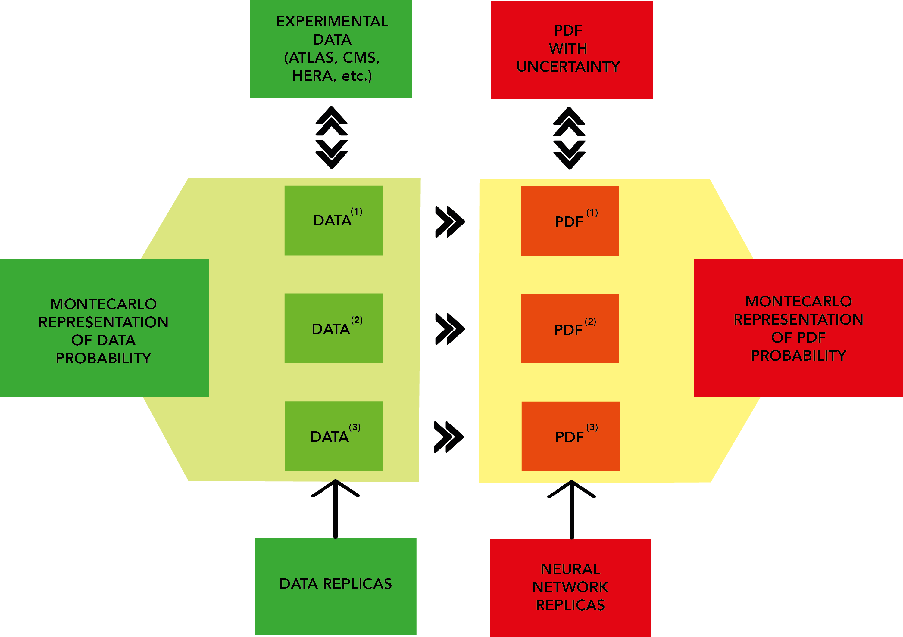
As seen in Sect. 1 the NNPDF methodology has the goal of determining the probability distribution of a set of functions, which in turn are related to the probability distributions of quantum events (the emission of a parton from a parent hadron) which provide the input to the computation of predictions for (discrete) experimental measurements. The methodology is based on two distinct ingredients: the use of a Monte Carlo representation for the probability distributions, and the use of neural networks as unbiased underlying interpolating functions. It is schematically represented in Figure 2.
The Monte Carlo representation provides a way of breaking down the problem of determining a probability in a space of functions into an (in principle infinite) set of problems in which a unique best-fit set of functions is determined. The basic idea is to turn the input probability distribution of data into a Monte Carlo representation. This means that the input data and correlated uncertainties are viewed as a probability distribution (typically, but not necessarily, a multigaussian) in the space of data, such that the central experimental values correspond to the mean and the correlated uncertainties correspond to the covariance of any two data. The Monte Carlo representation is obtained by extracting a set of replica instances from this probability distribution, in such a way that, in the limit of infinite number of replicas, the mean and and covariance over the replica sample reproduce the mean and covariance of the underlying distributions. In practice the number of replicas can be determined a posteriori by verifying that mean and covariance are reproduced to a given target accuracy.
A best-fit PDF (or rather, PDF set: i.e. one function for each distinct type of parton ) is then determined for each data replica, by minimization of a suitable figure of merit. Neural networks are used to represent the PDFs, with the value of as input, and the value of the PDF as an output (one for each PDF). Note that the fact that the data only depend indirectly on the input functions to be determined (the PDFs) is immaterial from the point of view of the general methodology. Indeed, the problem has been reduced to that of determining the optimal PDFs for each input data replica, namely, to standard training of neural networks. However, the fact that the PDF is not trained to the data directly will have significant implications on the nature of PDF uncertainties, on their validation, and on the optimization of PDF training, as we will discuss more extensively in Sections 3, 1, 2.
The output of the process is a set of PDF replicas, one for each data replica. These provide the desired representation of the probability density in the space of PDFs. Specifically, central values, uncertainties and correlations can be computed doing statistics over the space of PDF replicas: the best-fit PDF is the mean over the set of replicas, the uncertainty on any PDF for given can be found from the variance over the replica sample, and the correlation from the covariance.
The remaining methodological problems are how to determine the optimal neural network parametrization, how to determine the optimal PDF for each replica (i.e. the optimal neural network training) and how to validate the results. The way these issues are addressed in the current NNPDF methodology will be discussed in Section 2, while current work towards improving and hyperoptimizing the methodology are discussed in Section 3.
2 The state of the art
The NNPDF methodology, presented in Sect. 2, combines a Monte Carlo approach representation of probability distributions with neural networks as basic interpolants. Here we discuss first, the architecture of the neural networks, then their training, which is achieved by combining genetic minimization with stopping based on cross validation, and finally the validation of results through closure testing.
1 Neural networks for PDFs
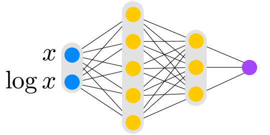
In all NNPDF determinations, starting with the proof-of-concept determination of a single PDF (isotriplet combination) in Ref. [9], up to and including the most recent global PDF set, NNPDF3.1 [12] the PDF architecture has been unchanged. Namely, PDFs are parameterized at a reference scale and expressed in terms of a set of independent neural networks multiplied by a preprocessing factor. Each of these neural networks consists of a fixed-size feed-forward multi-layer perceptron with architecture 2-5-3-1 (see Fig. 3). The only change in subsequent releases is in the number of independently parametrized PDFs (or PDF combinations), and thus of independent neural networks: one in the proof-of-concept Ref. [9], five in NNPDF1.0 [10] (up and down quarks and antiquarks and the gluon), seven from NNPDF1.1 [27], eight in NNPDF3.1 [12] (up, down, strange quarks and antiquarks; total charm; gluon).
The PDF momentum fraction enters the input layer nodes as , in order to account for the fact that the physical behavior of PDFs typically has two different regimes in the physically accessible region: a linear regime in the region and a logarithmic regime in the region . The next two hidden layers, with 5 and 3 nodes respectively, use the sigmoid activation function while the output node is linear. This particular choice of architecture was originally selected through systematic manual scans, as being sufficiently redundant to accommodate the PDF shape in an unbiased way .
The fact that it was never necessary to update this initial choice has validated the robustness of this analysis. Furthermore, in Ref. [10] it was explicitly checked that results would be unchanged if the number or nodes in the first hidden layer was reduced from 5 to 4. In Ref. [24], within a closure test (see Section 3 below), it was checked that results were unchanged if the number of the nodes in the intermediate layers was increased respectively from 5 to 20 and from 3 to 15, which corresponds to an increase of the number of free parameters of the neural net by more than one order of magnitude.
The parametrization for each PDF (or independent combination of PDFs) is
| (5) |
where is the neural network corresponding to a given combination . The quantities which are independently parametrized are the linear combination of light quark and gluon PDFs which correspond to eigenvectors of the PDF evolution equations, and charm: (see Refs. [14, 12] for the precise definition). is an overall normalization constant which enforces sum rules (such as the fact that the total momentum fractions carried by all partons must add up to one) and is a preprocessing factor which controls the PDF behavior at small and large .
The preprocessing exponents and were initially (NNPDF1.0 [10]) chosen to be fixed, while checking that no strong dependence of results was observed upon their variation. As the accuracy of the PDF determination improved, starting with NNPDF1.2 [28], in order to ensure unbiased results, the exponents were varied. Namely, the values of , were randomly selected for each PDF in each replica, with uniform distribution within a range fixed for each PDF, and kept fixed during the minimization of the replica. Effectively, with reference to Fig. 2, this means that for each PDF replicas the PDF parametrization is different, because the preprocessing function of each PDF is different. The range for each type of PDF (gluon, up quark, etc) was initially determined by requiring stability of the fit results, which, starting with NNPDF2.0 [11] was quantitatively determined by computing the correlation coefficient between the figure of merit (see Eq. (6) below) and verifying that it remained small. Starting with NNPDF3.0 [24], the range is now determined self-consistently: the effective exponents are computed for each independent combination of PDFs and for each PDF replica, the 68% confidence level range is determined for each combination, the fit is repeated with the exponents varied in a range taken equal to twice this range, and the procedure is iterated until the range stops changing.
As already mentioned, unlike in many standard regression problems, in which during the optimization procedure the model is compared directly to the training input data, in PDF fits the data are compared to theoretical predictions for physical observables of the form of Eq. (1), in which the PDFs are in turn obtained by solving a set of integro-differential equations from the PDFs , parametrized at the initial scale. Hence, the observable depends on the PDF through a number of convolution integrals, between the PDFs at scale , the evolution factors that take them to scale and the partonic cross sections of Eq. (1). In practice, the convolutions are turned into multiplication of pre-computed tables (FastKernel or FK-tables) by projecting on suitable basis functions, as discussed in Refs. [11, 29], see also Section 1 below.
2 The minimization procedure
The optimization procedure implemented in NNPDF consists in minimizing the loss function
| (6) |
where is the -th data point, is the convolution product between the FastKernel tables for point and the PDF model, and is the covariance matrix between data points and . The covariance matrix includes both uncorrelated and correlated experimental statistical and systematic uncertainties, as given by the experimental collaborations. Multiplicative uncertainties (such as normalization uncertainties), for which the uncertainty is proportional to the observable, must be handled through a dedicated method in order to avoid fitting bias: the method has been developed [30] to this purpose, and adopted from NNPDF2.0 [11] onward. Theory uncertainties (such as missing higher order uncertainties) could also be included as discussed in Refs. [31, 32] but this has only been done in preliminary PDF sets so far. Once again, we stress that input data are not provided for the neural networks, but rather for a complicated functional of the neural network output.
Genetic minimization
The minimization implemented in NNPDF3.1 and earlier releases is based on genetic algorithms (GA). Given that each PDF replica is completely independent from each other, the minimization procedure can be trivially parallelized. Genetic minimization was chosen for a number of reason. On the one hand, it was felt that that a deterministic minimization might run the risk of ending up in a local minimum related to the specific network architecture. Also, no efficient way of determining the derivative of the observables with respect to the parameters of the neural network was available then. In fact, modern, efficient deterministic minimization methods[33, 34] were not yet available at the time. As we will discuss in Section 1 below, these motivations are no longer valid and deterministic minimization is now more desirable.
The GA algorithm consists of three main steps: mutation, evaluation and selection. These steps are performed subsequently through a fixed number of iterations. The procedure starts with the initialization of the neural network weights for each PDF flavor using a random Gaussian distribution. From this initial network, a number of copies is produced, for which the weights are then mutated with a suitable rule. The mutations with lowest values of the figure of merit are selected and the procedure is iterated.
The GA initially adopted was based on point change mutations, in which individual weights or thresholds in the networks were mutated at random, according to a rule of the form
| (7) |
where is the -nth neural network weight or threshold, is a mutation rate size, is a uniform random number within [, ]. A fixed number of randomly chosen parameters are then mutated for each PDF, thereby producing a given number of mutants for each generation. The GA is fully specified by assigning: (i) the number of mutations for each PDFs; (ii) the mutation rates for each mutation and for each PDF; (iii) the number of mutants for each generation; (iv) the maximum number of generations. The mutation rates were dynamically adjusted as a function of the number of iterations according to
| (8) |
Several subsequent versions of this GA have been adopted. In a first version (NNPDF1.0 [10]), a fixed value of the number of mutations (two per PDF), of the number of mutants () and of the exponent () of Eq. (8) were adopted, with a small maximum number of generations (). At a later stage (NNPDF2.0 [11]) the minimization was divided in two epochs, with a transition at generations, and a larger number () of mutants in the first epoch, substantially decreased () in the second epoch; also the exponent was now randomly varied between 0 and 1 at each generation and the maximum number of generations was greatly increased (). At a yet later stage (NNPDF2.3 [35]) the number of mutations was increased to three for several PDFs.
Subsequent versions of the GA also involved various reweighting procedures, in which the contribution of different datasets to the figure of merit Eq. (6) was assigned a varying weight during the training, in order to speed up the training in the early stages. In a first implementation [10], these weights were computed as a ratio of the per datapoint for the given dataset, compared to the per datapoint of the worst-fitted dataset, so that best-fitted dataset would get less weight. Weights were then switched off when the value of the figure of merit fell below a given threshold. In a subsequent implementation [11], the weights were computed as ratios of the to a target value for the given dataset (determined from a previous fit) and only assigned to datasets for which the fit quality was worse than the target. Weights were only applied in a first training epoch.
Starting with NNPDF3.0 [24], a GA based on nodal mutation has been adopted. In nodal mutation, each node in each network is assigned an independent probability of being mutated. If a node is selected, its threshold and all of the weights are mutated according to Eqs. (7-8), with now fixed, and a random number between and shared by all of the weights. The values and mutation probability 15% per node have been selected as optimal based on closure tests (see Section 3 below). This algorithm proved to be significantly more efficient (see Figure 4 below) that the previous point mutation: in particular, reweighting is no longer necessary and it is no longer necessary to have different training epochs.
Stopping criterion
The GA presented in the previous Section 2 can lead to overfitting, in which not only the underlying law is fitted, but also statistical noise which is superposed to it. In order to avoid this, a stopping criterion is required. This was implemented since NNPDF1.0 through cross-validation. Namely, the data are separated in a training set, which is fitted, and a validation set, which is not fitted. The GA minimizes the of the training set, while the of the validation set is monitored along the minimization, and the optimal fit is achieved when the validation stops improving. This means that the fit optimizes the validation , which is not fitted. Because statistical noise is uncorrelated between the training and validation sets, this guarantees that overfitting of the statistical noise is avoided. Note that more subtle form of overfitting are possible, due to remaining correlations between training and validation sets: this, and the way to avoid it, will be discussed in Section 3 below.
In PDF fits before NNPDF3.0 [24] this stopping criterion was implemented by monitoring a moving average of the training and validation , and stopping when the validation moving average increased while the training moving average decreased by an amount which exceeded suitably chosen threshold values. This was necessary in order to avoid stopping on a local fluctuation, and it required the tuning of the moving average and of the threshold values, which was done by studying the typical fluctuations of the figure of merit. This clearly introduced a certain arbitrariness.
Since NNPDF3.0 [24], the previous stopping criterion has been replaced by the so-called look-back method. In this method, the PDF parametrization is stored for the iteration where the fit reaches the absolute minimum of the validation within a given maximum number of generations. This guarantees that the absolute minimum of the validation within the given maximum number of iterations is achieved. The method reduces the level of arbitrariness introduced in the previous strategy, but it requires reaching the maximum number of iterations for all replicas, out of which the absolute minimum is determined. This maximum must be chosen to be large enough that the absolute minimum is always reached, and it therefore leads on average to longer training. Adoption of this new stopping has been made possible thanks to greater computing efficiency.
3 Closure tests
As mentioned in Section 1 a critical issue in PDF determination is making sure that PDF uncertainties are faithful. Therefore, the validation of a PDF set chiefly consists of verifying that PDF uncertainties accurately reproduce the knowledge of the underlying true PDFs which has been learnt and stored, together with its uncertainty, in the Monte Carlo replica set through the training procedure. Because the true PDFs are not known, this can only be done through closure testing [36]. Namely, a particular underlying truth is assumed (in our case: a specific form for the true underlying PDFs); data are then generated based on this underlying truth; the methodology is applied to this data; results are finally compared to the underlying truth.
This exercise was performed for the NNPDF3.0 PDF set [24]; since the subsequent NNPDF3.1 PDF set [12] is based on the same methodology, this provides a validation of the current NNPDF PDF sets. In this Section we will briefly review the closure testing methodology and results of Ref. [24], while the ongoing validation of the new methodology of Section 3 will be discussed in Section 4 below.
In this closure test, data were generated by assuming that the underlying PDF has the form of the MSTW08 PDF set [37], and then generating a dataset identical to that used for the NNPDF3.0 PDF determination (about 4000 data points) but computing the hadronic cross sections using Eq. 1 with these PDFs adopted as input and the partonic cross sections determined using NLO QCD theory. Clearly, the exact form of the theory is immaterial if the same theory is used to generate the data and then to fit them, in such a way that only the fitting methodology is being tested. The independence of result on the particular choice of underlying truth can be explicitly tested by repeating the procedure with a different choice for the underlying PDF.
Besides providing a validation of the NNPDF methodology, the closure test also allows for an investigation of the sources of PDF uncertainty in a controlled setting. To this purpose, three sets of closure testing data were generated in Ref. [24]. The first set (“level 0”) consists of data generated with no uncertainties. This would correspond to a hypothetical case in which there are no experimental statistical or systematic uncertainties, so all data correspond to the “truth”, with vanishing uncertainty. A second set of data (“level 1”) is generated by assuming the probability distribution which corresponds to the published experimental covariance matrix. These data correspond to a hypothetical set of experimental results for which the experimental covariance matrix is exactly correct. A final set of data (“level 2”) is generated by taking the level 1 data as if they were actual experimental data, and then applying to them the standard NNPDF methodology, which, as discussed in Section 2 (See Figure 2) is based on producing a set of Monte Carlo replicas of the experimental data: the level 2 data are then the Monte Carlo replicas produced out of the level 1 data, as if the latter were actual experimental data.
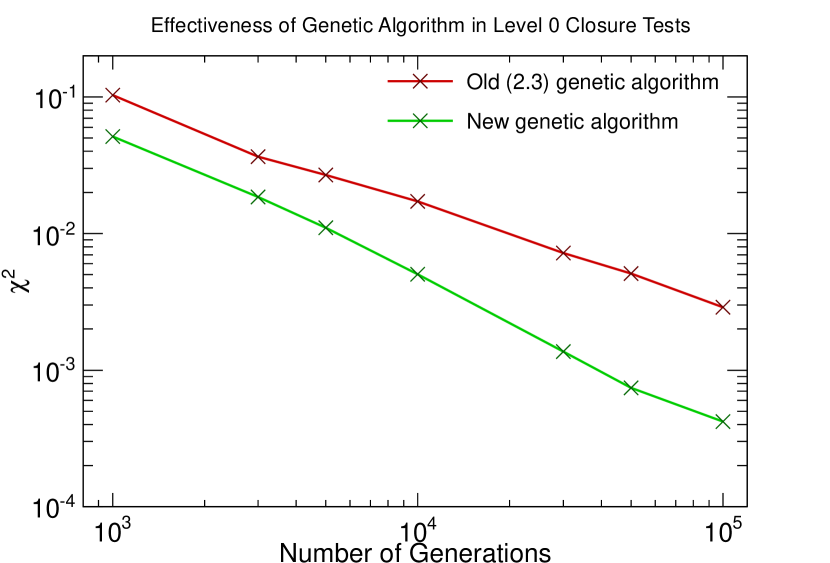
A first very simple test consists of fitting level 0 data, and computing the figure of merit ( per datapoint) as the training proceeds. Because these data have no uncertainty, a perfect fit with is in principle possible. Results are shown in Figure 4 for the two implementations of the minimization algorithm adopted in Refs. [35] (NNPDF2.3) and [24] (NNPDF3.0) and discussed in Section 2. Two sets of conclusions may be drawn from his plot. First, it is clear that the methodology is general and powerful enough to reproduce the underlying data: the figure of merit can be made arbitrarily small, which means that with vanishing experimental uncertainties, the data can be fitted with arbitrarily high accuracy. Second, it is possible to determine the dependence of the figure of merit on the training length, and specifically compare different minimization algorithms. Interestingly, Figure 4 shows that for the two GAs of Section 2 the figure of merit follows a power law: . Furthermore, it is clear that the value of is rather larger (faster convergence) for the NNPDF3.0 GA, based on nodal mutation (recall Section 2), in comparison to the previous NNPDF2.3 GA implementation.
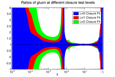
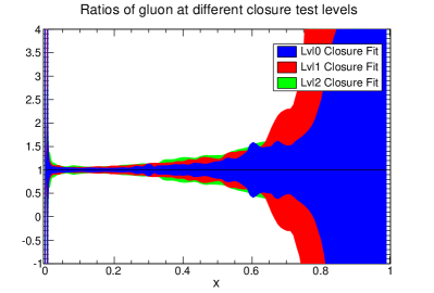
A second test compares the uncertainty on PDFs which is found when fitting respectively to level 0, level 1 and level 2 data. Results are shown for the gluon in Fig. 5: 68% confidence levels are shown for fits to level 0, level 1 and level 2 data. The plot has various implications. The first observation is that, as discussed in Section 1 the data constrain the PDFs only in a limited range (“data region”, henceforth). Outside that range the uncertainty grows very large, and in the absence of experimental information it is essentially arbitrary.
Coming now to the region where the experimental information is concentrated, note that when fitting level 0 and level 1 data the same datapoints are fitted over and over again, yet a spread of results is found. In the case of level 0 data we know from Figure 4 that the figure of merit on datapoints essentially vanishes (i.e., the fit goes through all datapoints with zero uncertainty). This then means that this unique minimum at the level of data does not correspond to a unique minimum at the level of PDFs: the datapoints are measurements of the hadronic cross section Eq. (1), which only indirectly depends on the PDFs . There is then a population of PDFs which lead to the same optimal fit because of the need to effectively interpolate between datapoints (“interpolation uncertainty”). Namely, even though at the data level there is a unique best fit, this does not correspond to a unique best-fit set of underlying PDFs.
At level 1 the datapoints are fluctuated about their true values, so the best-fit value of figure of merit on datapoints is now of order of per datapoint. The uncertainty is correspondingly increased because now there may be several PDF configurations which all lead to values of the figure of merit of the same order, possibly corresponding to different underlying functional forms for the PDFs (“functional uncertainty”). In other words, now the prediction is no longer uniquely determined even at the data level. Finally, at level 2, corresponding to a realistic situation, the data themselves fluctuate about the true value thereby inducing a “data uncertainty” on the PDFs.
Figure 4 shows that for the gluon in the data region these three components of the uncertainty are roughly of similar size. Note that, if a fixed functional form was fitted to the data by least-squares, both the level 0 and level 1 uncertainties would necessarily vanish. Hence, to the extent that the final level 2 uncertainty is faithful, a methodology based on a fixed functional form, for which level 0 and level 1 uncertainties vanish, necessarily leads to uncertainty underestimation.
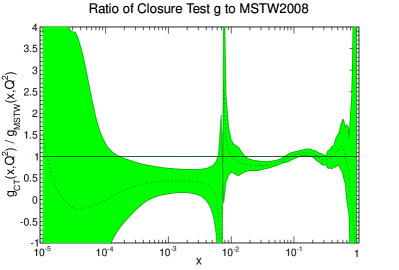
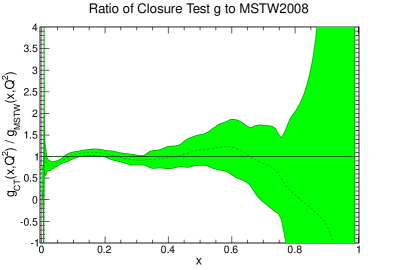
This begs the question of checking whether indeed the level 2 uncertainties, namely, the uncertainties found with standard NNPDF methodology are faithful. A first qualitative check can be done by simply comparing the final result to the underlying truth, which in a closure test is known. This is done for the gluon in Figure 6. It is clear that the result appears to be broadly consistent: the truth is mostly within the one- band, though not always, which is as it should be, given that the one- band is supposed to be a 68% confidence level. Note, however, that PDF values at neighboring points in are highly correlated: this is already true at the level of single replicas, but even more for the final PDF, obtained averaging over replicas, and it is of course as it should be – after all, if we were able to compute the PDF from first principles, it would be given by a unique functional form, most likely infinitely differentiable in the physical range. Hence, a confidence level cannot be computed by simply counting how many point in space fall within the one- band.
Rather, a quantitative check that the confidence level is correctly determined requires repeating the whole procedure several times. Namely, we need to check that if we regenerate a set of (level 1) experimental values, and then refit them, in of cases for each PDF at each point the true value falls within the one- uncertainty. More in general, the validation of the PDF determination requires first, computing PDFs and uncertainties from a given set of level 2 data, so the PDF and uncertainty are obtained by taking mean and covariance over replicas. Next, repeating the determination for different sets of level 2 data obtained from different primary level 1 data: for each fit one will obtain a different best-fit PDF set and corresponding uncertainties. Finally, computing the distribution of best-fit PDFs about the true value, and comparing this actual distribution of results about the truth with their nominal uncertainty.
In practice, the procedure is quite costly as it requires producing a large enough number of fits that confidence levels can be reliably computed, each containing a large enough set of PDF replicas that the PDF uncertainty can be reliably determined: for example, 100 sets of 100 PDF replicas each. In Ref. [24] this was done by introducing two approximations. First, the distribution of averages of level 2 replicas, each from a different set of level 1 data, was approximated with the distribution of fits of a single replica to unfluctuated level 1 data. Second, the uncertainty was assumed to be stable between different fits and was thus determined from a single 100-replica set to a particular set of level 2 data. The validity of these approximations will be further discussed in Sect. 4 below.
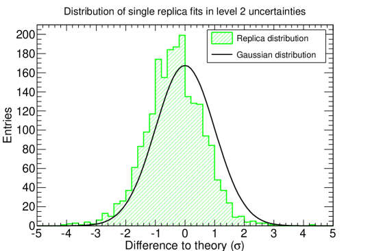
This procedure was used in Ref. [24] to compute the deviation of best-fit PDFs from the truth for all fitted PDFs evaluated at three values: , and , and respective uncertainties. The histogram of normalized deviations is compared to a univariate Gaussian in Figure 7. The deviation between the predicted and observed probability distribution are small: for instance, the one- confidence level is 69.9%, to be compared to the expected 68.3%. It is clear that the validation is successful.
The availability of closure test data allows performing a variety of further tests, all of which were done in Ref. [24]. On the one hand, it is possible to compare to the truth various features of the distribution of fitted PDFs, such as for example their arc-lengths, or the behavior of their probability distribution upon updating via Bayes’ theorem. On the other hand, it is possible to test the stability of results upon a number of variations of the methodology, such as the choice of architecture of the neural nets, the choice of GA and its parameters, the choice of PDF parametrization basis, the parameters of the cross-validation. Indeed, as mentioned in Section 1 it has been possible to check stability upon enlarging the architecture of the neural net, as mentioned ins Section 2 the method was used in order to optimize the parameters of the GA, and as mentioned above, it has been used to check the stability with respect to different choices of underlying truth.
3 The future of PDFs in a deep learning framework
The AI-based approach to PDF determination described in Section 2 largely eliminates potential sources of bias, specifically those related to the choice of a functional form, as discussed in Section 1, thanks to the universal nature of neural networks [38]. However, neural networks themselves are not unique, and the algorithms used for their training even less so. The methodology discussed in Section 2 has been developed over the years through a long series of improvements, as described in Sections 1-2. These were based on trial and error, and on the experience accumulated in solving a problem of increasing complexity. The human intervention involved in these choices might in turn be a source of bias. A way of checking whether this is the case, and then improving on the current methodology, is through hyperoptimization, namely, automatic optimization of the methodology itself. This goal was recently accomplished, but it required as a prerequisite a redesign of the NNPDF codebase, and specifically the replacement of the GA with deterministic minimization. Here we will discuss first, this code redesign, next the hyperoptimization procedure, then quality control, which plays a role analogous to cross-validation but now at the hyperoptimization level, and finally, the set of validation tests that ensure the reliability of the final hyperoptimized methodology.
1 A new approach based on deterministic minimization
The NNPDF methodology presented in Section 2 was implemented by the NNPDF collaboration as an in-house software framework relying on few external libraries. There are two major drawbacks of such an approach. First, the in-house implementation greatly complicates the study of novel architectures and the introduction of the modern machine learning techniques developed during the last decade. Second, the computational performance of GA minimization algorithms is a significant limitation, and it drastically reduces the possibility of performing hyperparameter scans systematically.
In order to overcome these problems the code has been redesigned using an object-oriented approach that provides the required functionality to modify and study each aspect of the methodology separately, and a regression model has been implemented from scratch in a modular object oriented approach based on external libraries. Keras [39] and TensorFlow [40] have been chosen as back-ends for neural network and optimization algorithms. This code design provides an abstract interface for the implementation of other machine learning oriented technologies, that simplifies maintainability and opens the possibility to new physics studies.
The new framework implements gradient descent (GD) methods to replace the previously used GA described in Section 2. Thanks to state-of-the art tools, this change reduces the computing cost of a fit while achieving similar or better goodness-of-fit. The GD methods produce more stable fits than their GA counterparts, and, thanks to the back-ends, the computation of the gradient of the loss function is efficient even when including the convolution with the FastKernel tables discussed in Section 1. Given the possibility of performing hyperoptimization scans, there is no longer a risk of ending up in architecture-dependent local minima.
In terms of neural networks, the new code uses just one single densely connected network as opposed to a separate network for each flavor. As previously done, we fix the first layer to split the input into the pair . We also fix 8 output nodes (one per flavor) with linear activation functions. Connecting all different PDFs we can directly study cross-correlation between the different PDFs not captured by the previous methodology.
As we change both the optimizer and the architecture of the network, the optimal setup must be re-tuned from scratch. To this purpose, we have implemented the hyperopt library [41], which allow us to systematically scan over many different combinations of hyperparameters finding the optimal configuration for the neural network. Therefore, the neural network architecture no longer has the form shown in Fig. 3: first, rather than a neural net per PDF, there is now a single neural net with as many outputs as are the independent PDFs, and second, the architecture (number of intermediate layers and number of nodes per layer) is now hyperoptimized, rather than being fixed.
In Fig. 8 we show a graphical representation of the full new methodology which will be referred to as n3fit in the sequel. The are vectors containing the -inputs of the neural network for each of the datasets entering the fit. These values of are used to compute both the value of the neural network and the preprocessing factor, thus determining the unnormalized PDF. The normalization constants (see Eq. (5)) are computed at every step of the fitting using the points. Recall from Section 1 that the PDFs are parametrized in a basis of linear combinations : individual PDFs for the quark flavors, antiflavors and the gluon, , are obtained through a rotation. This procedure concludes the necessary operations to compute the value of the PDF for any flavor at the reference scale .
All PDF parameters are stored in two blocks, the first named NN, namely the neural network of Eq. (5), and the preprocessing and . Given that each block is completely independent, we can swap them at any point, allowing us to study how the different choices affect the quality of the fit. All the hyperparameters of the framework are also abstracted and exposed. This specifically allows us to study several architectures hitherto unexplored in the context of PDF determination.
As repeatedly discussed in Sections 1-2, the PDFs are not compared directly to the data, but rather, predictions are obtained through a convolution over the neural networks. This, as mentioned in Section 1, is performed through the FastKernel method, which produces a set of observables from which the Eq. (6) can be computed. For this purpose, the first step is generation of a rank-4 luminosity tensor
| (9) |
where are flavor indices while label the index on the respective grids. Typical grids have of order of a hundred points in for each PDF, spaced linearly in at large , and logarithmically at small ; the grids are benchmarked and optimized in order to guarantee better than percent accuracy with high computational efficiency [11, 29, 12]. The physical observable, e.g. an inclusive cross-section or differential distribution, is then computed by contracting the luminosity tensor with the rank-5 FastKernel table for each separate dataset,
| (10) |
where corresponds to the index of the experimental data point within the dataset. This stage of the model is the most computationally intensive.
As discussed in Section 2, the optimal fit is determined through cross-validation. The cross-validation split, which takes the output and creates a mask for the training and validation sets, is introduced as a final layer. As mentioned, the training set is used for updating the parameters of the network during the fit while the validation set is monitored during the fit and only used for early stopping purposes. In Fig. 9 we present a schematic view of the stopping algorithm implemented in n3fit. The training is performed until the validation stops improving, from that point onward we enable a patience algorithm which waits for a number of iterations before raising the stopping action. For post-processing purposes we only accept stopping points for which the PDF produces positive predictions for a subset of pseudo data which tests the predictions for multiple processes in different kinematic ranges, see Refs. [24, 12] for further details.
The loss function Eq. (6) is minimized using gradient descent. Faster convergence and stability are found using algorithms with adaptive moment, in which the learning rate of the weights is dynamically modified, such as Adadelta [33], Adam [34] and RMSprop [43]. These three optimizers adopt similar gradient descent strategies, but differ in the prescription for weight update.
This approach has been applied to the baseline setup of the NNPDF3.1 NNLO PDF determination [12]: specifically, adopting the same dataset and cuts, together with the same fraction of validation data for cross-validation, though now the stopping criterion is different (Fig. 9). This setup, henceforth referred to as “global”, includes all datasets used in NNPDF3.1 NNLO, with 4285 data points. We also studied a reduced dataset which only includes data from deep-inelastic scattering (DIS), which is computationally less intensive, in particular because DIS is an electroproduction process, so the integral in Eq. (1) only involves a single PDF. This setup, called “DIS”, includes 3092 data points, and it facilitates the process of benchmarking and validation, since it leads to computationally very light fits, which allow us to extensively explore the parameter space.
Comparison of the average computing resources consumed by the old and new methodologies for the DIS and Global setups. DIS fit CPU h. Mem. Usage (GB) Good replicas n3fit (new) 0.2 2 95% nnfit (old) 4 4 70% Global fit CPU h. Mem. Usage (GB) Good replicas n3fit (new) 1.5 4 95% nnfit (old) 30 5 70%
In summary, the new methodology considerably improves the computational efficiency of PDF minimization, in particular because GD methods improve the stability of the fits, producing fewer bad replicas which need to be discarded, than theirs GA counterparts. This translates in a much smaller computing time. The old and new algorithms are compared in Table 1: we find a factor of 20 improvement with respect to the old methodology and near to a factor of 1.5 in the percentage of accepted replicas for a global fit setup. In terms of memory, in the old methodology usage is driven by the APFEL [44] code used in order to solve PDF evolution equations, which does not depend on the set of experiments being used. In the new code, evolution is never called during the fit (it is pre-computed in the fktables and then the final PDFs are evolved to all scales offline), so memory consumption is driven by the TensorFlow optimization strategy which in the case of hadronic data requires the implementation of Eq. (10) and its gradient. This difference translates to an important decrease on the memory usage of n3fit.
2 Optimized model selection
The main motivation for the development of the new optimized code discussed in Section 1 is the possibility of performing systematic explorations of the methodology through hyperoptimization. Firstly, the new design of the n3fit code exposes all parameters of the fit including the neural network architecture. This is of key importance for a proper hyperparameter scan where everything is potentially interconnected. Furthermore, the new methodology has such a smaller impact on computing resources that many more fits can be performed, with a difference by several orders of magnitude: for each fit using the old methodology hundreds of setups can now be tested.
The hyperparameter scan procedure has been implemented through the hyperopt framework [41], which systematically scans over a selection of parameter using Bayesian optimization [45], and measures model performance to select the best architecture. Table 2 displays an example of selection of scan parameters, subdivided into those which determine the Neural Network architecture, and those which control the minimization.
Parameters on which the hyperparameter scan is performed from [42]. Neural Network Fit options Number of layers Optimizer Size of each layer Initial learning rate Dropout Maximum number of epochs Activation functions Stopping Patience Initialization functions Positivity multiplier
Hyperparameter scans have been performed both in global and DIS setups. The best model configuration has been searched for, using as input data the original experimental values, rather than the data replicas which are then used for PDF determination (recall Section 2). Optimization has been performed using a combination of the best validation and stability of the fits: specifically, the architecture which produces the lowest validation has been selected after having trimmed combinations which displayed unstable behavior.
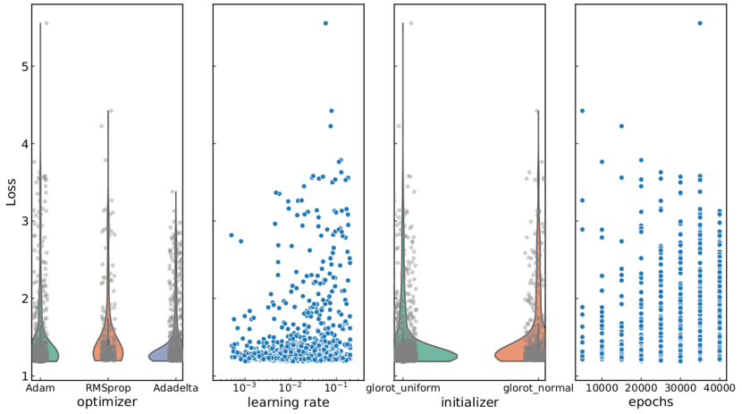
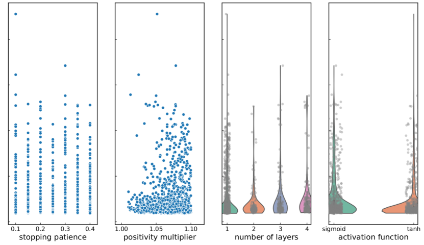
An example of scan for some of the parameters shown in Table 2, based the DIS setup, is shown in Fig. 10. The results of this scan can be summarized as follows. The Adadelta optimizer, for which no learning rate is used, is found to be more stable, and to systematically produce better results than RMSprop and Adam with a wide choice of learning rates. The initializers, once unstable options such as a random uniform initialization have been removed, seem to provide similar qualities with a slight preference for the “glorot_normal” initialization procedure described in Ref. [46]. Concerning the parameters related to stopping criteria, when the number of epochs is very small the fit can be unstable, however after a certain threshold no big differences are observed. The stopping patience shows a very similar pattern, stopping too early can be disadvantageous but stopping too late does not seem to make a big difference. The positivity multiplier, however, shows a clear preference for bigger values. Finally, concerning the neural network architecture, a small number of layers seems to produce slightly better absolute results, however, one single hidden layer seems to lead to poor results. Concerning the activation functions, the hyperbolic tangent seems to be slightly preferred over the sigmoid. Once an acceptable hyperparameter setup has been achieved, a final fine tuning was performed, as some of the choices could have been biased by a bad combination of the other parameters.
Clearly, the result of the hyperoptimization depends on the underlying dataset: for instance, we have verified that hyperoptimization on a very large global dataset prefers a larger architecture. Therefore, the reliability and stability of the hyperoptimized methodology have to be checked a posteriori, as we will discuss in Sect. 4.
In summary, hyperoptimization has been implemented as a semi-automatic methodology, that is capable of finding the best hyperparameter combination as the setup changes, e.g. with new experimental data, new algorithms or technologies.
3 Quality control
The hyperoptimization presented in Sect. 2 can be viewed as a meta-optimization in which the object of optimization is the methodology. This immediately raises the issue of quality control. In the fitting procedure, this is taken care by cross-validation, in which quality control is provided by the validation set. A similar quality control is now needed at the hyperoptimization level.
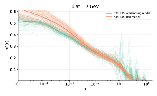
Indeed, if hyperoptimization is run by just optimizing on the validation figure of merit, a typical result is shown in Figure 11, in which replicas for the up quark PDF for a hyperoptimized DIS fit are shown. It is clear that an unstable behavior is seen, characteristic of overtraining. This can also be verified quantitatively: for example the value of the training is much lower than that of the validation . This may appear to be surprising, given that the hyperoptimization is performed on the validation , while the training is minimized in the fitting procedure. However, there inevitably exist correlations between the training and validation sets, for example through correlated theoretical and experimental uncertainties. Due to these correlations, hyperoptimization without quality control leads to overlearning.
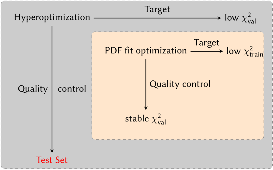
The problem can be solved by introducing a testing set, which tests the generalization power of the model. The testing set is made out of datasets which are uncorrelated to the training and validation data, and none of which is used in the fitting either for training or validation. The test set plays the role of quality control for the hyperoptimization, as schematically summarized in Figure 12.
Defining the best appropriate test dataset for PDF fits is particularly challenging due to the nature of the model regression through convolutions. Indeed, the choice of prescription for the test set presents a certain level of arbitrariness. For a first exploration, the test set has been constructed by utilizing datasets for which several experiments exist for the same process, and picking the experiment with smallest kinematic range. The corresponding data have been removed from training and validation, and used as a test set. A more refined option, which validates this first choice, will be discussed in Section 4 below.
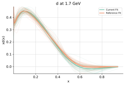
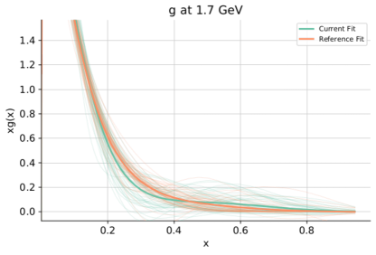
Best models found by our hyperparameter scan for the DIS and global setups using the new n3fit methodology. Parameter DIS only Global Hidden layers 2 3 Architecture 35-25-8 50-35-25-8 Activation tanh sigmoid Initializer glorot_normal glorot_normal Dropout 0.0 0.006 Optimizer Adadelta Adadelta Max epochs 40000 50000 Stopping patience 30% 30%
We have applied this procedure both to DIS and global fits. The best models found in each case are compared in Table 3. For the global setup deeper networks are allowed without leading to overfitting. The hyperbolic tangent and the sigmoid functions are found to perform similarly. The initializer of the weights of the network, however, carries some importance for the stability of the fits, with preference for the Glorot normal initialization method [46, 47] as implemented in Keras. Furthermore, adding a small dropout rate [48] to the hidden layers in the global fit reduces the chance of overlearning introduced by the deeper network, thus achieving more stable results. As expected, the bigger network shows a certain preference for greater waiting times (which also increases the stopping patience as is set to be a % of the maximum number of epochs). In actual fact, the maximum number of epochs is rarely reached and very few replicas are wasted.
Comparison of the total of the fit for both a DIS only and global fits found using the previous NNPDF3.1 and the new n3fit methodology. DIS only Global n3fit (new) 1.10 1.15 NNPDF3.1 (old) 1.13 1.16
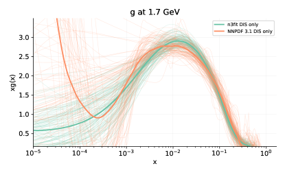
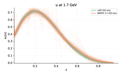
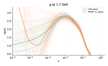
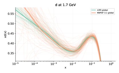
Turning now to fit results, despite the significant difference in size and complexity of the dataset, the DIS and global fits perform similarly in describing the experimental data, as demonstrated by the values presented in Table 3. It is interesting to compare results to those obtained using the previous NNPDF3.1 methodology. The total values are compared in Table 3: even though the new methodology leads to a slightly better fit, differences are small. PDF replicas obtained with either methodology (for the gluon and the up quark) are compared Fig. 13, both for the DIS and global fits. It is clear that the best-fit PDF, i.e. the average over replicas, is not much affected by the change in methodology (though somewhat smoother for nnfit).
A significant difference however is seen at the level of individual replicas: replicas found with the new methodology are rather more stable, i.e. they fluctuate rather less. This leads to slightly smaller uncertainties, and, more significantly, with the new methodology a smaller number of replicas is necessary in order to arrive to a stable average. The greater stability of the new methodology also leads to somewhat smaller uncertainties in the far extrapolation, i.e. in regions where there is no information and thus uncertainties are large: this is seen in Fig. 13 for the gluon distribution for . This raises the question of how to reliably assess uncertainties in extrapolation: we will return to this in Section 4 below.
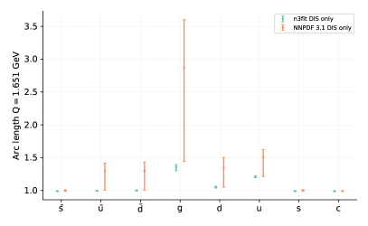
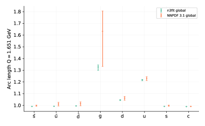
A particularly transparent way of seeing this greater stability is to compare PDF arc-lengths. Because a PDF is a function of , one may define the length of the curve traced by the PDF as varies in this interval. A very smooth PDF then has smaller arc-length. In Fig. 14 the mean and one- values of arclengths computed from a set of replicas with the new and old methodology are compared, both for the DIS and global fits. It is clear that, with the new methodology, the arc-length mean values are smaller, but especially the fluctuation of arc-length values between replicas is much smaller.
In summary we conclude that the new hyperoptimized n3fit methodology leads to results which are in broad agreement with the current NNPDF3.1 methodology, thereby confirming that the latter is faithful and unbiased, as expected based on the closure tests of Section 3. However, thanks to code redesign and deterministic minimization it is possible to achieve greater computational efficiency, and thanks to the hyperoptimization it is possible to obtain, based on the same underlying datasets, more stable results (i.e., a smaller number of replicas is sufficient to achieve good accuracy) and somewhat smaller uncertainties. In short, the new n3fit methodology, while providing a validation of the current NNPDF methodology, displays greater computational efficiency, greater stability and greater precision without loss of accuracy. This in turn calls for more detailed validation and testing, as we now discuss.
4 Validation and testing
The n3fit methodology motivates and enables more detailed studies of fit quality. It enables them because thanks to its much greater computational efficiency it is now possible to perform rather more detailed explorations than it was possible with the previous slower methodology. It motivates them, because the goal of the new methodology is to allow for greater precision without loss of accuracy, namely, to extract more efficiently the information contained in a given dataset. It is then mandatory to make sure that no new sources of arbitrariness are introduced by the new methodology. Also, the new methodology is claimed to be more precise without loss of accuracy, i.e. to produce results which are more stable and have smaller uncertainty than the previous methodology given the same input. It is then crucial to perform validation tests which are sufficiently detailed that the validity of this claim can be tested: in practice, this means tests that are sufficiently detailed that the two methodologies can be distinguished, and that impose more stringent requirements on the methodology itself.
We will first discuss the new issue of robustness of the test-set methodology introduced in Section 3, then turn to a more detailed set of closure tests, similar to those of Section 3 but now exploiting the new methodology, and finally discuss a new kind of test of the generalization power of the methodology: “future testing”.
Test-set stability
One new source of ambiguity in the n3fit methodology is the choice of an appropriate test set. Indeed, the setup discussed in Section 3 was based on a particular choice of test set, but one would like to avoid as much as possible this kind of potentially biased subjective choice. Also, in that setup one has to discard some data from the dataset used for fitting and only include them in the test set. This contrasts with the desire to keep data in the training set as much as possible, in order to exploit as much as possible the (necessarily limited) dataset in order to determine the wide variety of features of the underlying PDFs.
These goals can be achieved through a -fold cross-validation. In this algorithm, data are subdivide into partitions, each of which reproduces the broad features of the full dataset. Each of the partitions then plays in turn the role of the test set, by being excluded from the fit. A variety of figures of merit can then be chosen for hyperparameter optimization, such as the mean value of the loss over excluded partitions, or the best worst value of the validation loss of the excluded partition.
This -folding procedure has been implemented, and stability upon different choices of hyperoptimization figure of merit has been explicitly checked. Results are shown in Figure 15, where the best PDF models estimated using -folding are compared to those obtained through the simple test-set procedure of Section 3. Similar results are found using either method. While confirming the reliability of the manually selected method of Section 3, this allows us to replace it with the more robust and unbiased -folding method.
Closure testing
We now turn to closure testing, as presented in Section 3 in the context of NNPDF3.0 [24]. We have applied the closure testing methodology of Section 3, but now using the n3fit methodology and the more recent and wider NNPDF3.1 [12] dataset and theory settings. Hence, level 2 data are now in one-to-one correspondence with data in the NNPDF3.1 dataset, and, more importantly, we can take advantage of the greater computational efficiency of n3fit.
A first example of this is that it is now possible to perform confidence level tests based on actual full reruns. Indeed, recall from Section 3 that a computation of a closure test confidence level requires producing several independent fits, each with a sufficiently large number of replicas, so that the population of central values and uncertainties in each fit can be compared to an underlying truth. Thanks to the use of n3fit, it has now been possible to perform 30 different closure test level 2 fits, each with 40 replicas [50]. Results are then further enhanced and stabilized by using bootstrapping, i.e., by drawing random subsets of fits and random subsets of replicas from each fit and computing the various estimators for the resample of fits and replicas. It has been possible to check in this way that results are essentially stable with at least 10 fits with at least 25 replicas each, in that increasing the number of fits and replicas results are unchanged. All numbers quoted below refer to results obtained with the largest numbers of fits and replicas. The fact that such a relatively small number of replicas is sufficient to achieve stable result is a reflection of the greater stability of n3fit replicas discussed in Section 4.
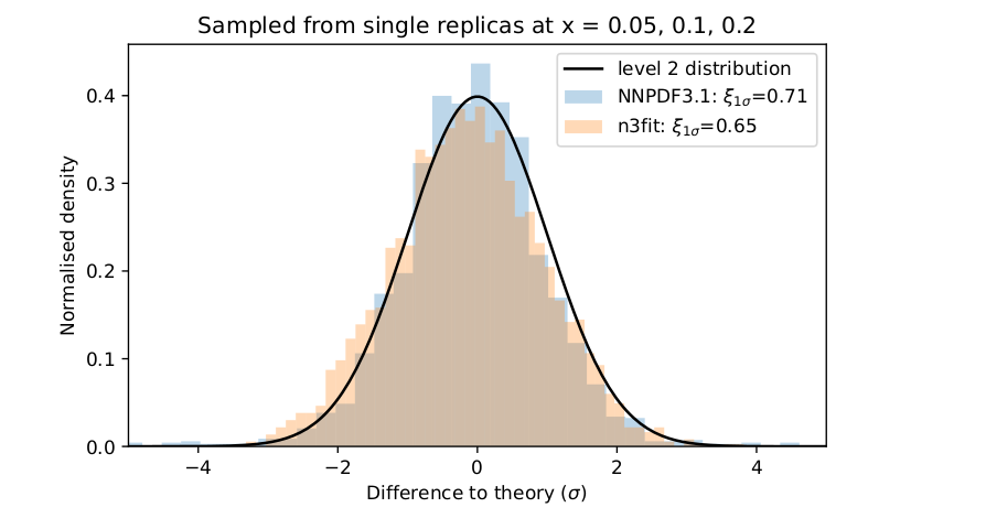
As a first test, we recompute the histogram of deviations of Figure 7, but now using NNPDF3.1 data. We can now compare the histogram actually computed using 30 fits with 40 replicas each, with the histogram approximately determined using a single 100 replica level 2 fit and 100 single-replica level 1 fits, as it was done for Figure 7 (labeled “NNPDF3.1 methodology”). The result is shown in Figure 16. It is clear that the validation is successful also for the (rather wider) NNPDF3.1 dataset: the one- confidence level now equal to 65%, and the mean of the histogram is now essentially unbiased, unlike in Figure 7 were a small bias was present. Also the approximate method used in Section 3 and Ref. [24] is reasonably accurate: specifically, the true value 65% is reasonably well approximated by the value 71% found using the approximate method.
We can now proceed to more detailed closure tests by computing confidence levels more extensively . A useful tool in this context is the bias-variance ratio. This, for Gaussian distributions, contains exactly the same information as the one- confidence level of predicted values with respect to the underlying truth considered in Section 3. For uncorrelated data, the bias-variance ratio is defined as the mean square deviation of the prediction from the truth (bias), divided by the expected one- uncertainty (variance). The square-root of the bias-variance ratio
| (11) |
(where , and are respectively the prediction, uncertainty and true value for the datapoint) is the ratio between observed and predicted uncertainties, and thus it should be equal to one for a perfect fit. The generalization to the correlated case is straightforwardly obtained by expressing the numerator and denominator under the square root in Eq. (11) in terms of the covariance matrix. We have verified explicitly that the value of the one- confidence level interval computed using the measured bias-variance ratio coincides with the measured confidence level, within statistical accuracy, so either can be equivalently used.
We can now turn to more detailed comparisons. First, the comparison can be done for each PDF individually, rather than for all PDFs lumped together. Second, the comparison can also be done at the level of experimental data: namely, instead of determining the deviation between the fitted and true PDF we determine the deviation between the prediction obtained using the best-fit PDF and the true PDF for each of the datapoints in the NNPDF3.1 dataset.
It should be noted that of course the predictions for individual datapoints are correlated due to the use of common underlying PDFs, with correlations becoming very high for datapoints which are kinematically close, so that the integral Eq. (1) is almost the same. These correlations can be simply determined by computing the covariance matrix between all datapoints induced by the use of the underlying PDFs, which in turn is done by determining covariances over the PDF replica sample. Confidence levels are then determined along eigenvectors of this covariance matrix, and can be compared to the bias-variance ratio, either by using its general form in the non-diagonal data basis, or equivalently, using Eq. (11) but with the sum running not on the original datapoints, but rather over the eigenvectors of the covariance matrix.
Of course, the PDFs themselves are also correlated. The histograms in Figures 7,16 were computed by sampling each PDF at three widely spaced points in so as to minimize this correlation, but of course computing a histogram of deviations with correlations neglected is still an approximation. When performing comparisons in PDF space we have now therefore also computed the covariance between PDFs over the replica sample, and determined confidence intervals along its eigenvectors, and the corresponding bias-variance ratio values with correlations kept into account.
A first comparison has been performed by computing the bias-variance ratio at the data level. This leads to an interesting result. Recall from Section 3 and Figure 5 that the total PDF uncertainty consists of three components of comparable side, the first of which is due to the need to interpolate between data. Clearly, this latter component is absent if one compares the prediction to the same data which have been used to produce the PDF set. Indeed, we find that the square root of the bias-variance ratio computed for the NNPDF3.1 dataset (more than 4000 datapoints) is . If we compute the same ratio for a new wide dataset including about 1300 HERA, LHCB, ATLAS and CMS data not used in the fit we find that the value is . The difference between these two values can be understood as an indication of the fact that in the former case the bias does not include the level 1 uncertainty, while the variance (which should be used for new prediction) does. The value means that PDF uncertainties on predictions are accurate to 10% (and somewhat overestimated).
We next computed both the bias-variance ratio and the one-sigma confidence level at the PDF level. PDFs have been sampled at four points for each PDF, in a region in corresponding to the data region, and the covariance matrix has been subsequently diagonalized as discussed above. Results are shown in Table 4 for individual PDF combinations. It is clear that, especially for the PDF combinations that are known with greater accuracy, such as the quark singlet and the gluon , uncertainties are faithful: only the combination which measures the total strangeness shows a certain amount of uncertainty underestimation, by about 30%.
Chronological future tests
The closure tests essentially verify the reliability of results in the data region. A much more difficult task is to verify the power of generalization of the methodology: namely, whether PDFs determined with a subset of data are able to correctly predict the behavior of new data, including those that extend the kinematic domain used for PDF determination. In practice, this means testing whether PDF uncertainties are reliable also in regions in which they start growing significantly because of lack of information.
This is done by “chronological” or “future” tests. Namely, we consider an existing (or hypothetical) past dataset, we train PDFs based on it, and we compare the best-fit results with later data which extend the kinematic region. A first test of this kind has been performed only including data which predated the HERA electron-proton collider, and which thus approximately correspond to the information on PDFs available around 1995. This is especially interesting since it is well known (see e.g. [51]) that the best-fit gluon shape substantially changed after the advent of HERA data, as pre-HERA data impose only very loose constraints on the gluon PDF.
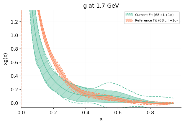
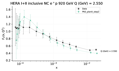
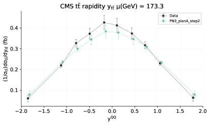
We have thus produced a PDF determination using n3fit methodology, but only including pre-HERA data, and now performing a dedicated hyperparameter optimization based on this restricted dataset. The best-fit gluon determined in this way is compared to the current best-fit gluon in Figure 17. Some subsequent data which are sensitive to the gluon, specifically the proton structure function , which is sensitive to the gluon at small , and top-pair production at the LHC, which is sensitive to the gluon at medium-high , are compared to predictions obtained using this PDF set in Figure 18.
It is clear that the test is successful. In the region , where the gluon is currently known accurately thanks to HERA data, but it is extrapolated when only using pre-HERA data, the uncertainty grows very large, yet the two fits are compatible within these large uncertainties, and the new data are within the uncertainty of the extrapolated prediction. This is a highly nontrivial test of the generalizing power of the hyperoptimized n3fit methodology. Note also that this provides us with a test of the stability of the hyperoptimized methodology, in that it means that a methodology hyperoptimized to the much larger current dataset leads to reliable results even when used on the much more restrictive past dataset.
The optimization of the generalization power of our methodology is at the frontier of our current understanding and remains a challenging open problem.
5 Outlook
The n3fit methodology will be used in the construction of future PDF releases, starting with the forthcoming NNPDF4.0 PDF set. The greater efficiency of this methodology will be instrumental in dealing with an ever increasing data set, while its greater accuracy will be instrumental in reaching the percent-level uncertainty goal which is likely required for discovery at the HL-LHC [25]. Avenues of research for future methodological developments which are currently under consideration include the possibility of an integrated reinforcement learning framework for the development of an optimal PDF methodology, the exploration of machine learning tools alternative to neural networks, such as Gaussian processes, the exploration of inference tools, such as transfer learning, for the modeling of theoretical uncertainties, and a deeper understanding of the generalizing power of the methodology outside the data region.
Acknowledgments
We thank all the past and current members of the NNPDF collaboration and the members of the N3PDF team, whose work is behind most of the results reported here, for collaboration and for countless stimulating discussions, and in particular Rosalyn Pearson for a reading of the first draft. We acknowledge financial support from the European Research Council under the European Union’s Horizon 2020 research and innovation Programme (grant agreement n. 740006).
References
- 1. R. McElhaney and S. F. Tuan, Some consequences of a modified Kuti Weisskopf quark parton model, Phys. Rev. D8 (1973) 2267.
- 2. T. Kawaguchi and H. Nakkagawa, “Analysis of Scaling Violation in Terms of Theories with Anomalous Dimensions.” KUNS 380, 1976.
- 3. A. De Rujula, H. Georgi, and H. D. Politzer, Demythification of Electroproduction, Local Duality and Precocious Scaling, Ann. Phys. 103 (1977) 315.
- 4. P. W. Johnson and W.-k. Tung, Comparison of Asymptotically Free Theories with High- Energy Deep Inelastic Scattering Data, Nucl. Phys. B121 (1977) 270.
- 5. M. Gluck and E. Reya, Operator Mixing and Scaling Deviations in Asymptotically Free Field Theories, Phys. Rev. D14 (1976) 3034.
- 6. I. Hinchliffe and C. H. Llewellyn Smith, Detailed Treatment of Scaling Violations in Asymptotically Free Gauge Theories, Nucl. Phys. B128 (1977) 93.
- 7. S. Forte, L. Garrido, J. I. Latorre, and A. Piccione, Neural network parametrization of deep inelastic structure functions, JHEP 05 (2002) 062, arXiv:hep-ph/0204232 [hep-ph].
- 8. NNPDF, L. Del Debbio, S. Forte, J. I. Latorre, A. Piccione, and J. Rojo, Unbiased determination of the proton structure function f2(p) with faithful uncertainty estimation, JHEP 03 (2005) 080, hep-ph/0501067.
- 9. NNPDF, L. Del Debbio, S. Forte, J. I. Latorre, A. Piccione, and J. Rojo, Neural network determination of parton distributions: The nonsinglet case, JHEP 03 (2007) 039, arXiv:hep-ph/0701127.
- 10. NNPDF, R. D. Ball, L. Del Debbio, S. Forte, A. Guffanti, J. I. Latorre, A. Piccione, J. Rojo, and M. Ubiali, A Determination of parton distributions with faithful uncertainty estimation, Nucl. Phys. B 809 (2009) 1, arXiv:0808.1231 [hep-ph]. [Erratum: Nucl.Phys.B 816, 293 (2009)].
- 11. R. D. Ball, L. Del Debbio, S. Forte, A. Guffanti, J. I. Latorre, J. Rojo, and M. Ubiali, A first unbiased global NLO determination of parton distributions and their uncertainties, Nucl. Phys. B838 (2010) 136, arXiv:1002.4407 [hep-ph].
- 12. NNPDF, R. D. Ball et al., Parton distributions from high-precision collider data, Eur. Phys. J. C77 (2017) 10, 663, arXiv:1706.00428 [hep-ph].
- 13. R. K. Ellis, W. J. Stirling, and B. R. Webber, QCD and collider physics. Cambridge University Press, 1996.
- 14. S. Forte, Parton distributions at the dawn of the LHC, Acta Phys. Polon. B 41 (2010) 2859, arXiv:1011.5247 [hep-ph].
- 15. J. Gao, L. Harland-Lang, and J. Rojo, The Structure of the Proton in the LHC Precision Era, Phys. Rept. 742 (2018) 1, arXiv:1709.04922 [hep-ph].
- 16. J. J. Ethier and E. R. Nocera, Parton Distributions in Nucleons and Nuclei, Ann. Rev. Nucl. Part. Sci. (2020) 70, 1, arXiv:2001.07722 [hep-ph].
- 17. H.-W. Lin et al., Parton distributions and lattice QCD calculations: toward 3D structure, arXiv:2006.08636 [hep-ph].
- 18. R. G. Roberts, The Structure of the proton: Deep inelastic scattering. Cambridge University Press, 1990.
- 19. CTEQ, H. L. Lai et al., Global QCD analysis of parton structure of the nucleon: CTEQ5 parton distributions, Eur. Phys. J. C12 (2000) 375, arXiv:hep-ph/9903282.
- 20. T.-J. Hou et al., New CTEQ global analysis of quantum chromodynamics with high-precision data from the LHC, arXiv:1912.10053 [hep-ph].
- 21. D. Stump, J. Pumplin, R. Brock, D. Casey, J. Huston, J. Kalk, H. Lai, and W. Tung, Uncertainties of predictions from parton distribution functions. 1. The Lagrange multiplier method, Phys. Rev. D 65 (2001) 014012, arXiv:hep-ph/0101051.
- 22. J. Pumplin, D. Stump, R. Brock, D. Casey, J. Huston, J. Kalk, H. Lai, and W. Tung, Uncertainties of predictions from parton distribution functions. 2. The Hessian method, Phys. Rev. D 65 (2001) 014013, arXiv:hep-ph/0101032.
- 23. A. D. Martin, R. G. Roberts, W. J. Stirling, and R. S. Thorne, Uncertainties of predictions from parton distributions. I: Experimental errors. ((T)), Eur. Phys. J. C28 (2003) 455, arXiv:hep-ph/0211080.
- 24. NNPDF, R. D. Ball et al., Parton distributions for the LHC Run II, JHEP 04 (2015) 040, arXiv:1410.8849 [hep-ph].
- 25. P. Azzi et al., Report from Working Group 1: Standard Model Physics at the HL-LHC and HE-LHC, vol. 7, pp. 1–220. 12, 2019. arXiv:1902.04070 [hep-ph].
- 26. E. Bagnaschi and A. Vicini, A new look at the estimation of the PDF uncertainties in the determination of electroweak parameters at hadron colliders, arXiv:1910.04726 [hep-ph].
- 27. NNPDF, J. Rojo, R. D. Ball, L. Del Debbio, S. Forte, A. Guffanti, J. I. Latorre, A. Piccione, and M. Ubiali, Update on Neural Network Parton Distributions: NNPDF1.1, in 38th International Symposium on Multiparticle Dynamics. 2009. arXiv:0811.2288 [hep-ph].
- 28. NNPDF, R. D. Ball, L. Del Debbio, S. Forte, A. Guffanti, J. I. Latorre, A. Piccione, J. Rojo, and M. Ubiali, Precision determination of electroweak parameters and the strange content of the proton from neutrino deep-inelastic scattering, Nucl. Phys. B 823 (2009) 195, arXiv:0906.1958 [hep-ph].
- 29. V. Bertone, S. Carrazza, and N. P. Hartland, APFELgrid: a high performance tool for parton density determinations, Comput. Phys. Commun. 212 (2017) 205, arXiv:1605.02070 [hep-ph].
- 30. NNPDF, R. D. Ball, L. Del Debbio, S. Forte, A. Guffanti, J. I. Latorre, J. Rojo, and M. Ubiali, Fitting Parton Distribution Data with Multiplicative Normalization Uncertainties, JHEP 05 (2010) 075, arXiv:0912.2276 [hep-ph].
- 31. R. Abdul Khalek et al., A First Determination of Parton Distributions with Theoretical Uncertainties, arXiv:1905.04311 [hep-ph].
- 32. NNPDF, R. Abdul Khalek et al., Parton Distributions with Theory Uncertainties: General Formalism and First Phenomenological Studies, Eur. Phys. J. C 79 (2019) 11, 931, arXiv:1906.10698 [hep-ph].
- 33. M. D. Zeiler, ADADELTA: An Adaptive Learning Rate Method, arXiv:1212.5701 [cs.LG].
- 34. D. P. Kingma and J. Ba, Adam: A Method for Stochastic Optimization, arXiv:1412.6980 [cs.LG].
- 35. R. D. Ball et al., Parton distributions with LHC data, Nucl. Phys. B 867 (2013) 244, arXiv:1207.1303 [hep-ph].
- 36. L. Demortier, Proceedings, PHYSTAT 2011 Workshop on Statistical Issues Related to Discovery Claims in Search Experiments and Unfolding, CERN,Geneva, Switzerland 17-20 January 2011, ch. Open Issues in the Wake of Banff 2011. 2011.
- 37. A. D. Martin, W. J. Stirling, R. S. Thorne, and G. Watt, Parton distributions for the LHC, Eur. Phys. J. C63 (2009) 189, arXiv:0901.0002 [hep-ph].
- 38. G. Cybenko Math. Control Signal Systems 2 (1989) 303.
- 39. F. Chollet et al., “Keras.” https://keras.io, 2015.
- 40. M. Abadi, A. Agarwal, P. Barham, E. Brevdo, Z. Chen, C. Citro, G. S. Corrado, A. Davis, J. Dean, M. Devin, S. Ghemawat, I. Goodfellow, A. Harp, G. Irving, M. Isard, Y. Jia, R. Jozefowicz, L. Kaiser, M. Kudlur, J. Levenberg, D. Mané, R. Monga, S. Moore, D. Murray, C. Olah, M. Schuster, J. Shlens, B. Steiner, I. Sutskever, K. Talwar, P. Tucker, V. Vanhoucke, V. Vasudevan, F. Viégas, O. Vinyals, P. Warden, M. Wattenberg, M. Wicke, Y. Yu, and X. Zheng, “TensorFlow: Large-scale machine learning on heterogeneous systems.” Software available from tensorflow.org, 2015. http://tensorflow.org/.
- 41. J. Bergstra, D. Yamins, and D. D. Cox, Making a science of model search: Hyperparameter optimization in hundreds of dimensions for vision architectures, in Proceedings of the 30th International Conference on International Conference on Machine Learning - Volume 28, ICML’13. JMLR.org, 2013. http://dl.acm.org/citation.cfm?id=3042817.3042832.
- 42. S. Carrazza and J. Cruz-Martinez, Towards a new generation of parton densities with deep learning models, Eur. Phys. J. C79 (2019) 8, 676, arXiv:1907.05075 [hep-ph].
- 43. T. Tieleman and G. Hinton, “Lecture 6.5—RmsProp: Divide the gradient by a running average of its recent magnitude.” Coursera: Neural networks for machine learning, 2012.
- 44. V. Bertone, S. Carrazza, and J. Rojo, APFEL: A PDF Evolution Library with QED corrections, Comput. Phys. Commun. 185 (2014) 1647, arXiv:1310.1394 [hep-ph].
- 45. J. Bergstra, R. Bardenet, Y. Bengio, and B. Kégl, Algorithms for hyper-parameter optimization, in Proceedings of the 24th International Conference on Neural Information Processing Systems, NIPS’11. Curran Associates Inc., USA, 2011. http://dl.acm.org/citation.cfm?id=2986459.2986743.
- 46. X. Glorot and Y. Bengio, ”understanding the difficulty of training deep feedforward neural networks”, in In Proceedings of the International Conference on Artificial Intelligence and Statistics (AISTATS’10). Society for Artificial Intelligence and Statistics. 2010.
- 47. Y. Bengio and X. Glorot, ”understanding the difficulty of training deep feed forward neural networks”, International Conference on Artificial Intelligence and Statistics (01, 2010) 249.
- 48. G. E. Hinton, N. Srivastava, A. Krizhevsky, I. Sutskever, and R. Salakhutdinov, Improving neural networks by preventing co-adaptation of feature detectors, CoRR abs/1207.0580 (2012) , arXiv:1207.0580. http://arxiv.org/abs/1207.0580.
- 49. NNPDF in preparation.
- 50. L. Del Debbio and M. Wilson in preparation.
- 51. W.-K. Tung, Status of global QCD analysis and the parton structure of the nucleon, in 12th International Workshop on Deep Inelastic Scattering (DIS 2004). 9, 2004. arXiv:hep-ph/0409145.