PBHs and secondary GWs from ultra slow roll and punctuated inflation

Abstract

The primordial scalar power spectrum is well constrained by the cosmological data on large scales, primarily from the observations of the anisotropies in the cosmic microwave background (CMB). Over the last few years, it has been recognized that a sharp rise in power on small scales will lead to enhanced formation of primordial black holes (PBHs) and also generate secondary gravitational waves (GWs) of higher and, possibly, detectable amplitudes. It is well understood that scalar power spectra with COBE normalized amplitude on the CMB scales and enhanced amplitudes on smaller scales can be generated due to deviations from slow roll in single, canonical scalar field models of inflation. In fact, an epoch of so-called ultra slow roll inflation can lead to the desired amplification. We find that scenarios that lead to ultra slow roll can be broadly classified into two types, one wherein there is a brief departure from inflation (a scenario referred to as punctuated inflation) and another wherein such a departure does not arise. In this work, we consider a set of single field inflationary models involving the canonical scalar field that lead to ultra slow roll and punctuated inflation and examine the formation of PBHs as well as the generation of secondary GWs in these models. Apart from considering specific models, we reconstruct potentials from certain functional choices of the first slow roll parameter leading to ultra slow roll and punctuated inflation and investigate their observational signatures. In addition to the secondary tensor power spectrum, we calculate the secondary tensor bispectrum in the equilateral limit in these scenarios. Moreover, we calculate the inflationary scalar bispectrum that arises in all the cases and discuss the imprints of the scalar non-Gaussianities on the extent of PBHs formed and the amplitude of the secondary GWs generated. We conclude with a discussion on the wider implications of our results.

I Introduction

With the recent observations of gravitational waves (GWs) from merging binary black holes involving a few to tens of solar masses [1, 2, 3, 4, 5, 6, 7, 8, 9, 10, 11, 12], there has been a considerable interest in examining whether such black holes could have a primordial origin [13, 14, 15]. The most popular mechanism to generate primordial black holes (PBHs) is the inflationary scenario (for earlier discussions, see, for example, refs. [16, 17]; also see the recent reviews [18, 19, 20, 21]). PBHs are formed when the curvature perturbations generated during inflation reenter the Hubble radius during the radiation and matter dominated epochs. However, most inflationary models permit only slow roll inflation and, in such cases, the extent of PBHs produced proves to be considerably smaller than required for any astrophysical implications (see, for example, ref. [22]). Recall that, on large scales, the primordial scalar power spectrum is strongly constrained by the increasingly precise observations of the anisotropies in the cosmic microwave background (CMB) (for recent constraints from Planck, see refs. [23, 24]). In order to lead to a significant amount of PBHs, the scalar power spectrum on small scales should be considerably enhanced from the COBE normalized values over the CMB scales (for an early discussion in this context, see, for instance, ref. [22]). In inflation, this is possible only when there are strong departures from slow roll. It boils down to identifying inflationary potentials that permit slow roll initially and then violating it for a certain period of time, before restoring it again until close to the termination of inflation.

In models of inflation driven by a single, canonical scalar field, the so-called ultra slow scenario has turned out to be the most popular mechanism in the literature to enhance scalar power on small scales. This scenario involves a period during inflation wherein the first slow roll parameter turns very small (for the initial discussions, see refs. [25, 26, 27]; in this context, also see, for instance, refs. [28, 29]). In fact, one finds that the scenario can be further divided into two types, those which admit a brief period of departure from inflation and another wherein no such departure arises. The scenario wherein inflation is interrupted briefly is referred to as punctuated inflation (for the original discussions, see refs. [30, 31, 32]; for later and recent efforts, see refs. [33, 34, 35, 36]; for a discussion in the context of PBHs, see refs. [37, 28]). Interestingly, in such scenarios, the interruption of inflation is inevitably followed by an epoch of ultra slow roll which aids in boosting the power on small scales. While, in the case of punctuated inflation, all the slow roll parameters (including the first) turn large briefly, in ultra slow roll inflation, the first slow parameter remains small until the very end of inflation and slow roll is said to be violated due to the large values achieved by the second and higher slow roll parameters.

Often, the above-mentioned scenarios are achieved with the aid of potentials which contain a point of inflection [34, 35, 25, 26, 27, 29]. The inflection point seems to play a crucial role in these scenarios in inducing a period of ultra slow roll after the short epoch of deviation from slow roll. The two stages of slow roll and ultra slow roll lead to either a step or a bump-like feature in the resulting inflationary scalar power spectrum, depending on the details of the intermediate departure from slow roll. The lower level of the step is associated with the large scale modes that leave the Hubble radius during the first epoch of slow roll and the power is enhanced on small scales corresponding to modes that leave the Hubble radius during the later epoch of ultra slow roll. We should mention here that the punctuated inflationary scenario has been considered to explain the lower power observed at the small multipoles in the CMB data. If one chooses the drop in power to occur at scales roughly corresponding to the Hubble radius today, one finds that the resulting power spectrum can improve the fit to the CMB data to a certain extent (for an earlier analysis, see ref. [34]; for a recent discussion, see ref. [36]).

We mentioned above that both ultra slow roll inflation and punctuated inflation can lead to a sharp rise in power on small scales. Evidently, if one chooses the rise to occur at suitable scales, one can utilize these power spectra to lead to enhanced formation of PBHs. As has been established, such an enhanced amplitude for the scalar power spectrum can induce secondary GWs when these modes reenter the Hubble radius at later times during the radiation dominated epoch (for the original discussions, see, for example, refs. [38, 39, 40, 41]; for recent discussions in this context, see refs. [42, 43, 44]). These secondary GWs with boosted amplitudes can, in principle, be detected by current and forthcoming observatories such as LIGO/Virgo [45], Pulsar Timing Arrays (PTA) [46, 47, 48], the Laser Interferometer Space Antenna (LISA) [49, 50], the Big Bang Observer (BBO) [51, 52, 53], the Deci-hertz Interferometer Gravitational wave Observatory (DECIGO) [54, 55] and the Einstein Telescope (ET) [56, 57]. Moreover, the deviations from slow roll inflation, even as they boost the scalar power spectrum on small scales, also lead to larger levels of scalar non-Gaussianities on these scales (in this context, see, for example, refs. [58, 59, 60]). These non-Gaussianities can, in principle, further increase the extent of PBH formation (for early discussions, see, for example, refs. [22, 61, 62]; for recent discussions, see refs. [63, 64, 65, 66, 67, 68, 69, 70]) as well as the strength of the secondary GWs (see refs. [71, 72, 73]; for a very recent discussion, also see ref. [74]). In this work, we examine the enhanced formation of PBHs and the generation of secondary GWs in ultra slow roll and punctuated inflation. We also numerically evaluate the inflationary scalar bispectrum generated on small scales in these scenarios and utilize the results to discuss the corresponding imprints on the extent of PBHs formed and the amplitude of secondary GWs. In addition to considering specific potentials that lead to the scenarios of our interest, we choose functional forms for the first slow roll parameter leading to ultra slow roll and punctuated inflation, reverse engineer potentials and examine the observational implications (for other efforts in these directions, see, for instance, Refs. [22, 75, 76, 77]). Interestingly, such an exercise also confirms the understanding that, in models of inflation involving a single, canonical scalar field, a point of inflection in the potential seems essential to lead to ultra slow roll or punctuated inflation.

This paper is organized as follows. In the following section, we shall introduce the different models of our interest which lead to ultra slow roll and punctuated inflation. In section III, we shall discuss the power spectra that arise in these models and illustrate how the intrinsic entropy perturbation associated with the scalar field proves to be responsible for enhancing the amplitude of the curvature perturbations. In this section, we shall also highlight some of the challenges that one encounters in constructing viable models of ultra slow roll and punctuated inflation. In section IV, we shall consider specific forms for the first slow roll parameter leading to ultra slow roll and punctuated inflation, and reverse engineer the potentials that lead to such scenarios. We shall also discuss the power spectra that arise in these cases. In sections V and VI, we shall discuss extent of PBHs formed and calculate the dimensionless parameters characterizing the power as well as bispectra of secondary GWs generated in the models and scenarios of interest. We shall also compare our results with the constraints from observations. In section VII, we shall calculate the dimensionless non-Gaussianity parameter $f_{{}_{\rm NL}}$ associated with the scalar bispectrum in all the different cases. We shall highlight some of the properties of the non-Gaussianity parameter $f_{{}_{\rm NL}}$ and then go on to discuss the imprints of the scalar non-Gaussianities on the formation of PBHs and the generation of secondary GWs. In section VIII, we shall conclude with a summary of the main results. We shall relegate some of the related discussions to six appendices.

A few remarks on our conventions and notations are in order at this stage of our discussion. We shall work with natural units such that $\hbar=c=1$ and set the reduced Planck mass to be $M_{{}_{\mathrm{Pl}}}=\left(8\,\pi\,G\right)^{-1/2}$. We shall adopt the signature of the metric to be $(-,+,+,+)$. Note that Latin indices shall represent the spatial coordinates, except for $k$ which shall be reserved for denoting the wave number. We shall assume the background to be the spatially flat Friedmann-Lemaître-Robertson-Walker (FLRW) line element described by the scale factor $a$ and the Hubble parameter $H$. Also, an overdot and an overprime shall denote differentiation with respect to the cosmic time $t$ and the conformal time $\eta$, respectively. Moreover, $N$ shall denote the number of e-folds.

II Models of ultra slow roll and punctuated inflation

In this section, we shall briefly describe the specific models of interest that lead to ultra slow roll and punctuated inflation. We should mention that all the five models that we shall discuss in the following two subsections contain a point of inflection. Recall that, the first slow roll parameter is defined as $\epsilon_{1}=-\dot{H}/H^{2}$. The higher order slow roll parameters are defined in terms of the first slow roll parameter $\epsilon_{1}$ through the relations

$$\epsilon_{n+1}=\frac{{\mathrm{d}}\,\mathrm{ln}\,\epsilon_{n}}{{\mathrm{d}}N}$$ (1)

for $n\geq 1$. As it is the first three slow roll parameters, viz. $\epsilon_{1}$, $\epsilon_{2}$, and $\epsilon_{3}$, that determine the amplitude and shape of the power spectrum as well as the bispectrum, we shall illustrate the behavior of these slow roll parameters in the models of interest.

II.1 Potentials leading to ultra slow roll inflation

We shall consider two specific models that permit ultra slow roll inflation. The first potential we shall consider which leads to a period of ultra slow roll inflation is often written in the following form (see, for instance, ref. [25]):

$$V(\phi)=V_{0}\;\frac{6\,x^{2}-4\,\alpha\,x^{3}+3\,x^{4}}{(1+\beta\,x^{2})^{2}},$$ (2)

where $x=\phi/v$, with $v$ being a constant rescaling factor. We shall work with the following choices of the parameters involved: $V_{0}/M_{{}_{\mathrm{Pl}}}^{4}=4\times 10^{-10}$, $v/M_{{}_{\mathrm{Pl}}}=\sqrt{0.108}$, $\alpha=1$ and $\beta=1.4349$. For these choices of parameters, the inflection point, say, $\phi_{0}$, is located at $0.39\,M_{{}_{\mathrm{Pl}}}$. We find that, if we choose the initial value of the field to be $\phi_{\mathrm{i}}=3.614\,M_{{}_{\mathrm{Pl}}}$, then inflation lasts for about $63$ e-folds in the model. For convenience, we shall hereafter refer to the potential (2), along with the above-mentioned set of parameters, as USR1.

The second potential that we shall consider is given by [28]

$$V(\phi)=V_{0}\,\left\{\mathrm{tanh}\left(\frac{\phi}{\sqrt{6}\,M_{{}_{\mathrm{Pl}}}}\right)+A\,\sin\left[\frac{\mathrm{tanh}\left[\phi/\left(\sqrt{6}\,M_{{}_{\mathrm{Pl}}}\right)\right]}{f_{\phi}}\right]\right\}^{2},$$ (3)

and we shall work with the following values of the parameters involved: $V_{0}/M_{{}_{\mathrm{Pl}}}^{4}=2\times 10^{-10}$, $A=0.130383$ and $f_{\phi}=0.129576$. We find that, for these values of the parameters, the inflection point occurs at $\phi_{0}=1.05\,M_{{}_{\mathrm{Pl}}}$. For the initial value of the field $\phi_{\mathrm{i}}=6.1\,M_{{}_{\mathrm{Pl}}}$, we obtain about $66$ e-folds of inflation in the model. We shall refer to the potential (3) and the above set of parameters as USR2.

As we mentioned, the background dynamics driven by these potentials can be well captured by the behavior of the first three slow roll parameters $\epsilon_{1}$, $\epsilon_{2}$ and $\epsilon_{3}$. We have plotted the evolution of these quantities as a function of e-folds $N$ in figure 1.

Figure 1: The behaviors of the first three slow roll parameters $\epsilon_{1}$ (on top), $\epsilon_{2}$ (in the middle) and $\epsilon_{3}$ (at the bottom) have been plotted in the models of interest which lead to ultra slow roll and punctuated inflation. We have plotted the behaviors for all the five models we have discussed, viz. USR1 and USR2 (as solid and dashed curves, on the left) as well as PI1, PI2 and PI3 (as solid, dashed and dotted curves, on the right). Note that all the models consist of two distinct regimes of slow roll and ultra slow roll inflation, while the punctuated inflationary models also contain a short period of departure from inflation.

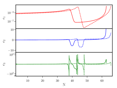
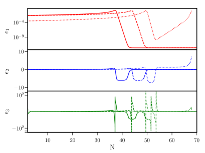
It is clear from the behavior of $\epsilon_{1}$ that these models permit two different regimes of slow roll, separated by a short phase of departure from slow roll. Note that the value of $\epsilon_{1}$ during the second regime of slow roll is a few orders of magnitude smaller than its value during the initial regime, thereby leading to the nomenclature of ultra slow roll inflation. We should point out that there is no deviation from inflation in these models, as the first slow roll parameter always remains smaller than unity until the very end of inflation. The transition from slow roll to ultra slow roll is rather rapid and this aspect is reflected by the sharp rise and fall in the amplitude of the second and third slow roll parameters within a short period. It should also be highlighted that the second slow roll parameter $\epsilon_{2}$ is large and negative (about $-6$ and $-7$ in USR1 and USR2) during the ultra slow phase when the first slow roll parameter $\epsilon_{1}$ is rapidly decreasing. The parameter $\epsilon_{2}$ changes sign when $\epsilon_{1}$ begins to rise as the field crosses the point of inflection and rolls down towards the minimum of the potential. But, $\epsilon_{2}$ continues to remain relatively large (it is about $0.2$ and $0.9$ in the cases of USR1 and USR2) even during this latter phase, when compared to the typical slow roll values encountered, say, at early times before the transition to the epoch of ultra slow roll.

To gain a better understanding of the dynamics involved, in figure 2, we have also plotted the evolution of the scalar field in phase space for the case of USR2.

Figure 2: The dynamics of the scalar field in the phase space $\phi$-$\phi_{N}$, where $\phi_{N}={\mathrm{d}}\phi/{\mathrm{d}}N$, has been illustrated for the models USR2 (on the left) and PI3 (on the right). Apart from the trajectory for the specific initial conditions we shall be working with (plotted in red), we have also plotted the evolution for a few other initial conditions (as solid curves in different colors). Moreover, in the case of the primary trajectory, we have indicated the lapse in time every $3$ e-folds (as black dots on the red curves). Further, we have highlighted the evolution arrived at using the standard slow roll approximation (as dotted blue curves). Note that the vertical lines (in dashed black) identify the point of inflection.

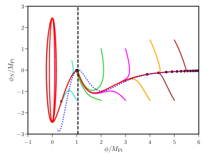
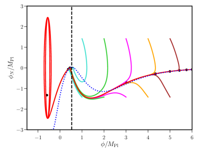
Evidently, trajectories from different initial conditions eventually merge with the primary trajectory of interest. The transition to the ultra slow roll regime corresponds to the sharp upward turn in the phase space trajectory when the velocity of the field decreases as it nears the point of inflection. It is interesting to note that the solution obtained in the slow roll approximation closely follows the primary trajectory even during the ultra slow roll regime. The field crosses the point of inflection, eventually emerging from the ultra slow regime, and inflation ends as the field approaches the minimum of the potential.

II.2 Potentials permitting punctuated inflation

As we have discussed, punctuated inflation corresponds to a scenario wherein a short period of departure from inflation is sandwiched between two epochs of slow roll. With the help of specific examples, we shall illustrate that the period of departure from inflation is inevitably followed by an epoch of ultra slow roll inflation.

A simple model that has been examined in the early literature which permits interrupted inflation is described by the potential (see ref. [30]; also see refs. [31, 32])

$$V(\phi)=V_{0}\,\left(1+B\,\phi^{4}\right).$$ (4)

It should be evident that the inflection point for this model is located at $\phi=0$. For $B/M_{{}_{\mathrm{Pl}}}^{4}=0.5520$, one finds that the model leads to two epochs of inflation separated by a brief interruption of inflation. In fact, around the interruption, the first slow roll parameter rises above unity and quickly falls to very small values, resulting in a period of ultra slow roll. It is easy to argue that such a behavior arises due to the constant term $V_{0}$ in the potential [30]. But, the presence of the constant term simultaneously leads to an important drawback of the model. Once inflation is restored after the interruption, it is found that the eventual slow roll regime lasts forever. There is no conventional termination of inflation as the constant term $V_{0}$ sustains slow roll evolution even when the field has reached the bottom of the potential. So, one is either forced to terminate inflation by hand or invoke an additional source to end inflation. Despite these drawbacks, we shall nevertheless briefly discuss the model due to its simplicity. We shall work with the above-mentioned value for the parameter $B$ and choose $V_{0}/M_{{}_{\mathrm{Pl}}}^{4}=8\times 10^{-13}$. We shall set the initial value of the field to be $\phi_{\mathrm{i}}=17\,M_{{}_{\mathrm{Pl}}}$, and we shall assume that inflation ends after $70$ e-folds. We shall hereafter refer to this model as PI1.

The second potential that we shall consider can be expressed as (see, for instance, refs. [78, 34, 35])

$$V(\phi)=\frac{m^{2}}{2}\,\phi^{2}-\left(\frac{\sqrt{2\,\lambda\,(n-1)}\,m}{n}\right)\,\phi^{n}+\frac{\lambda}{4}\,\phi^{2\,(n-1)},$$ (5)

where $n$ is an integer. These potentials contain a point of inflection at

$$\phi_{0}=\left[\frac{2\,m^{2}}{\lambda\,(n-1)}\right]^{1/[2\,(n-2)]}.$$ (6)

We shall focus on the case $n=3$, wherein the potential above reduces to

$$V(\phi)=\frac{m^{2}}{2}\,\phi^{2}-\frac{2\,m^{2}}{3\,\phi_{0}}\,\phi^{3}+\frac{m^{2}}{4\,\phi_{0}^{2}}\,\phi^{4},$$ (7)

and we shall work with the following values of the parameters: $m/M_{{}_{\mathrm{Pl}}}=1.8\times 10^{-6}$ and $\phi_{0}/M_{{}_{\mathrm{Pl}}}=1.9777$. As we shall soon discuss, these choice of parameters indeed admit punctuated inflation. However, one finds, as in the case of PI1, the above potential (for the parameters mentioned) does not naturally result in an end of inflation. Despite this limitation, we shall discuss the model, since, it should be clear that, modulo the denominator, the potential describing USR1 [cf. eq. (2)] is essentially the same as the potential (5). We shall choose the initial value of the field to be $\phi_{\mathrm{i}}=20\,M_{{}_{\mathrm{Pl}}}$, and we shall again assume that inflation ends after $70$ e-folds. We shall refer to this model as PI2.

Another model we shall consider that permits punctuated inflation is motivated by supergravity. It is described by the potential (see ref. [28]; for a very recent discussion, also see ref. [79])

$$V(\phi)=V_{0}\,\left[c_{0}+c_{1}\,\tanh\,\left(\frac{\phi}{\sqrt{6\,\alpha}}\right)+c_{2}\,\tanh^{2}\left(\frac{\phi}{\sqrt{6\,\alpha}}\right)+c_{3}\,\tanh^{3}{\left(\frac{\phi}{\sqrt{6\,\alpha}}\right)}\right]^{2},$$ (8)

and we shall work with the following values for the parameters involved: $V_{0}/M_{{}_{\mathrm{Pl}}}^{4}=2.1\times 10^{-10}$, $c_{0}=0.16401$, $c_{1}=0.3$, $c_{2}=-1.426$, $c_{3}=2.20313$ and $\alpha=1$. This model too contains a point of inflection and, for the above values for the parameters, the inflection point is located at $\phi_{0}=0.53\,M_{{}_{\mathrm{Pl}}}$. If we choose the initial value of the field to be $\phi_{\mathrm{i}}=7.4\,M_{{}_{\mathrm{Pl}}}$, we find that inflation ends after about $68$ e-folds. We shall refer to this model as PI3. For the above choice of the parameters, apart from a plateau for large field values, the potential admits a second plateau at smaller values of the field. As we shall see soon, it is these aspects of the potential that permits punctuated inflation and thereby aids in boosting the scalar power spectrum at small scales.

As in the case of the ultra slow roll models we had discussed in the previous sub-section, we have plotted the first three slow roll parameters $\epsilon_{1}$, $\epsilon_{2}$ and $\epsilon_{3}$ for the models PI1, PI2 and PI3 in figure 1. It is easy to see from the plots that the behavior of the three slow roll parameters are very similar across the models and they differ only in their location of the departures from slow roll. Evidently, after an initial slow roll regime, a brief departure from inflation occurs with $\epsilon_{1}$ growing above unity. The interruption of inflation is immediately followed by a period of ultra slow roll with $\epsilon_{1}$ falling to a value that is considerably smaller than its value during the initial slow roll regime. Moreover, other than PI3, the models have no definite end of inflation since $\epsilon_{1}$ does not rise to unity once the ultra slow roll regime has begun. Further, note that, when the epoch of ultra slow roll sets in, as in USR1 and USR2, the second slow roll parameter $\epsilon_{2}$ turns large and negative in all the cases of PI1, PI2 and PI3. The parameter $\epsilon_{2}$ eventually approaches zero in the cases of PI1 and PI2, since the first slow roll parameter never rises from its very low values in these models. However, in PI3, since $\epsilon_{1}$ rises ultimately leading to the end of inflation, the second slow roll parameter $\epsilon_{2}$ eventually turns positive (from nearly $-7$) and attains a large value (around $1.2$), in very much the same manner it had in USR2. As with USR2, we have plotted the behavior of the field in phase space for the case of PI3 in figure 2. It should be clear from the figure that the velocity of the field reaches larger values in the case of PI3 than in the case of USR2 prior to entering the ultra slow roll regime. Evidently, it is this behavior that is responsible for the brief interruption of inflation.

III Evolution of the curvature perturbation and power spectra

In this section, we shall discuss the scalar and tensor power spectra that arise in the models permitting ultra slow roll and punctuated inflation we had introduced in the previous section. However, before we go on to discuss the power spectra, we shall illustrate the behavior of the curvature perturbations during the period of deviation from slow roll. Specifically, we shall highlight the role played by the intrinsic entropy perturbations in the enhancement of the amplitude of the curvature perturbations over wave numbers that leave the Hubble radius either immediately prior to or during the departure from slow roll.

III.1 Scalar and tensor modes, and power spectra

Let ${\mathcal{R}}$ and $\gamma_{ij}$ denote the curvature and the tensor perturbations at the first order, respectively. Also, let ${\mathcal{R}}_{\bm{k}}$ and $\gamma_{ij}^{\bm{k}}$ denote the Fourier modes associated with these perturbations. Recall that the modes ${\mathcal{R}}_{\bm{k}}$ and $\gamma_{ij}^{\bm{k}}$ satisfy the differential equations

$${\mathcal{R}}_{\bm{k}}^{\prime\prime}+2\,\frac{z^{\prime}}{z}\,{\mathcal{R}}_{\bm{k}}^{\prime}+k^{2}\,{\mathcal{R}}_{\bm{k}} = 0,$$ (9a)

$${\gamma_{ij}^{\bm{k}}}^{\prime\prime}+2\,\frac{a^{\prime}}{a}\,{\gamma_{ij}^{\bm{k}}}^{\prime}+k^{2}\,\gamma_{ij}^{\bm{k}} = 0,$$ (9b)

where $z=\sqrt{2\,\epsilon_{1}}\,M_{{}_{\mathrm{Pl}}}\,a$, with $\epsilon_{1}$ being the first slow roll parameter. Moreover, note that, if $\hat{{\mathcal{R}}}_{\bm{k}}$ and $\hat{\gamma}_{ij}^{\bm{k}}$ denote the operators associated with the scalar and tensor modes on quantization, the scalar and tensor power spectra $\mathcal{P}_{{}_{\mathrm{S}}}(k)$ and $\mathcal{P}_{{}_{\mathrm{T}}}(k)$ are defined in terms of these operators through the relations

$$\langle\hat{{\mathcal{R}}}_{{\bm{k}}}(\eta_{\rm e})\,{\hat{\mathcal{R}}}_{{\bm{k}}^{\prime}}(\eta_{\rm e})\rangle = \frac{2\,\pi^{2}}{k^{3}}\;{\cal P}_{{}_{\rm S}}(k)\;\delta^{(3)}\left({\bm{k}}+{\bm{k}}^{\prime}\right),$$ (10a)

$$\langle\,{\hat{\gamma}}_{ij}^{{\bm{k}}}(\eta_{\rm e})\,\hat{\gamma}^{ij}_{{\bm{k}}^{\prime}}(\eta_{\rm e})\,\rangle = \frac{2\,\pi^{2}}{k^{3}}\,{\mathcal{P}}_{{}_{\rm T}}(k)\;\delta^{(3)}({\bm{k}}+{\bm{k}}^{\prime}),$$ (10b)

where $\eta_{\rm e}$ is the conformal time at late times, close to the end of inflation. We should mention that, in the above expressions, the expectation values on the left hand side are to be evaluated in the specified initial quantum state, which we shall assume to be the Bunch-Davies vacuum. Let $f_{k}$ and $g_{k}$ denote the positive frequency modes (associated with the Bunch-Davies vacuum) in terms of which the operators $\hat{{\mathcal{R}}}_{\bm{k}}$ and $\hat{\gamma}_{ij}^{\bm{k}}$ are decomposed. Then, in terms of the quantities $f_{k}$ and $g_{k}$, the power spectra $\mathcal{P}_{{}_{\mathrm{S}}}(k)$ and $\mathcal{P}_{{}_{\mathrm{T}}}(k)$ can be expressed as

$$\mathcal{P}_{{}_{\mathrm{S}}}(k) = \frac{k^{3}}{2\,\pi^{2}}\,|f_{k}(\eta_{\rm e})|^{2},$$ (11a)

$$\mathcal{P}_{{}_{\mathrm{T}}}(k) = 8\,\frac{k^{3}}{2\,\pi^{2}}\,|g_{k}(\eta_{\rm e})|^{2}.$$ (11b)

III.2 Role of the intrinsic entropy perturbation

Often the evolution of the curvature perturbations in non-trivial scenarios involving departures from slow roll inflation are examined in terms of the behavior of the quantity $z$ (see, for instance, Refs. [28, 80, 81]). We find that it proves to be instructive to understand this aspect from the behavior of the intrinsic entropy perturbations [31, 33]. It is well known that, in contrast to perfect fluids, scalar fields, in general, possess non-vanishing non-adiabatic pressure perturbation $\delta p_{{}_{\mathrm{NA}}}$ or, equivalently, the intrinsic entropy perturbation ${\mathcal{S}}$, which are related through the expression (in this context, see, for example, refs. [82, 83])

$$\delta p_{{}_{\mathrm{NA}}}=\frac{p^{\prime}}{\mathcal{H}}\,{\mathcal{S}},$$ (12)

where $p$ denotes the pressure associated with the background and $\mathcal{H}=a\,H$ is the conformal Hubble parameter. In the case of inflation driven by a single, canonical scalar field, one can show that the intrinsic entropy perturbation ${\mathcal{S}}_{k}$ associated with a given mode of the field can be expressed in terms of the corresponding curvature perturbation, say, ${\mathcal{R}}_{k}$, as follows [31, 33]:

$${\mathcal{R}}_{k}^{\prime}=-\left[\frac{2\,a^{2}\,p^{\prime}}{M_{{}_{\mathrm{Pl}}}^{2}\,(\mathcal{H}^{\prime}-\mathcal{H}^{2})}\right]\,\left(\frac{1}{1-c_{{}_{\mathrm{A}}}^{2}}\right)\,{\mathcal{S}}_{k},$$ (13)

where $c_{{}_{\mathrm{A}}}=\sqrt{p^{\prime}/\rho^{\prime}}$ is adiabatic speed of the scalar perturbations, with $\rho$ being the background energy density. It is easy to show using the equation of motion (9a) describing the curvature perturbation that, in the super Hubble limit, the intrinsic entropy perturbation ${\mathcal{S}}_{k}$ decays as $\mathrm{e}^{-2\,N}$. However, it is found that, during deviations from slow roll, for modes which are either about to leave or have just left the Hubble radius, the amplitude of the intrinsic entropy perturbation briefly increases, sourcing the curvature perturbation [32, 33]. This, in turn, alters the amplitude of the curvature perturbation for modes which cross the Hubble radius just before or during the departure from slow roll.

To demonstrate these effects, in figure 3, we have plotted the evolution of the curvature and the intrinsic entropy perturbations in the inflationary models USR2 and PI3.

Figure 3: The evolution of the amplitudes of the imaginary parts of the curvature perturbation ${\mathcal{R}}_{k}$ (on the left) and the corresponding intrinsic entropy perturbation ${\mathcal{S}}_{k}$ (on the right) have been plotted for the three wave numbers $k=10^{10}\,\mathrm{Mpc}^{-1}$, $10^{11}\,\mathrm{Mpc}^{-1}$ and $10^{14}\,\mathrm{Mpc}^{-1}$ (in light, lime and dark green, respectively) in the two models USR2 (on top) and PI3 (at the bottom) as a function of e-folds. We have also included the behavior of the first two slow roll parameters $\epsilon_{1}$ and $|\epsilon_{2}|$ (in red and blue, respectively, on the left) in these models to indicate the regime (demarcated by the cyan band) over which the transition from slow roll to ultra slow roll occurs. The first mode with the smallest wave number is already in the super-Hubble regime when the departure from slow roll sets in, and the amplitude of the corresponding curvature perturbation is hardly affected by the transition. The second mode is barely in the super-Hubble regime when the transition from slow roll begins. The amplitude of its curvature perturbation is slightly attenuated as it emerges from the departure from slow roll. Whereas, the amplitude of the curvature perturbation associated with the third mode, which leaves the Hubble radius right in the middle of the transition, exhibits a considerable enhancement due to the transition. These changes in the curvature perturbations can be attributed to the rapid growth in the corresponding entropy perturbations (plotted on the right) during the transition. We find that ${\mathcal{S}}_{k}$ grows as either $\mathrm{e}^{3\,N}$ or $\mathrm{e}^{4\,N}$ (indicated as dashed lines) during the transition. We also find that the entropy perturbations eventually die down as $\mathrm{e}^{-2\,N}$ in the super-Hubble limit (indicated by dotted lines) as expected. It is these behaviors that lead to features in the inflationary scalar power spectra.

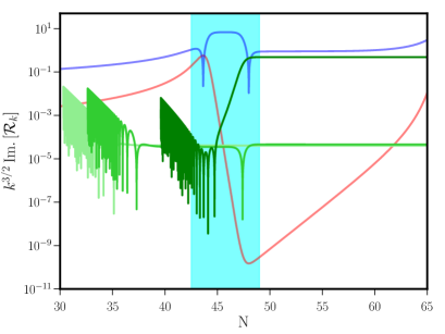
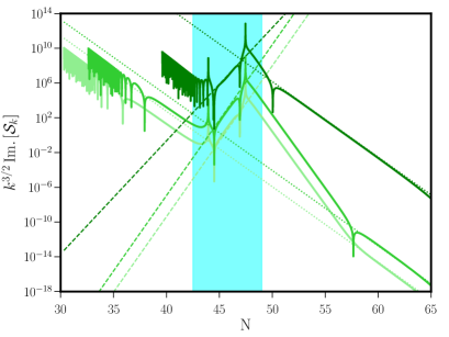
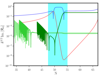
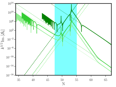
In order to highlight the differences in the behavior of the modes, we have plotted the evolution of the amplitudes for three modes which leave the Hubble radius just prior to the start of the departure from slow roll inflation, immediately after start of the period of transition, and during the middle of the transition. We should point out that we have plotted the imaginary parts of ${\mathcal{R}}_{k}$ and ${\mathcal{S}}_{k}$ since they dominate at late times. Moreover, they allow us to highlight the oscillations in the sub-Hubble regime. The time when these oscillations cease is an indication that the modes have crossed the Hubble radius. Evidently, there is a sharp rise in the amplitude of the intrinsic entropy perturbation for all the modes during the departure from slow roll inflation. We should add here that the corresponding real parts of ${\mathcal{R}}_{k}$ and ${\mathcal{S}}_{k}$ behave in a roughly similar manner. It is the sharp rise in ${\mathcal{S}}_{k}$ that is responsible for either an enhancement or a suppression in the asymptotic (i.e. late time) amplitude of the curvature perturbation, thereby leading to features in the power spectrum (for related discussions in this context, also see, for instance, refs. [28, 84]). In contrast, we find that there is relatively little effect of the deviation from slow roll on the evolution of the amplitude of the tensor perturbations. Due to this reason, the tensor power spectrum exhibits far less sharper features than the scalar power spectrum.

III.3 Scalar and tensor power spectra

We shall now turn to the scalar and tensor power spectra that arise in the ultra slow roll and punctuated inflationary scenarios we had discussed in the last section. Barring the brief rise of $\epsilon_{1}$ above unity in the models of punctuated inflation and the location of the deviations from slow roll inflation, we had seen that the behavior of the first three slow roll parameters were very similar in the different models of our interest (cf. figure 1). We can expect these features to be reflected in the corresponding power spectra. In figure 4, we have plotted the power spectra arising in all the five models, viz. USR1, USR2, PI1, PI2 and PI3.

Figure 4: The scalar (in red) and tensor power spectra (in blue) have been plotted in the various ultra slow roll and punctuated inflationary models of our interest — USR1 and USR2 (as solid and dashed curves, on top) and PI1, PI2, and PI3 (as solid, dashed and dotted curves, at the bottom) — over a wide range of scales. Note that the enhancement of power on small scales is more in the case of USR2 than USR1. Moreover, in the case of the punctuated inflationary models, the scalar power in PI1 and PI2 do not eventually come down at very small scales due to the fact that inflation does not terminate in these models. We should also point out that, in contrast to the scalar power spectra, the tensor power spectra have lower power at small scales when compared to the large scales.

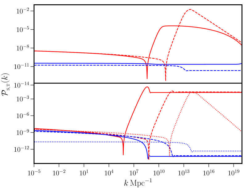
We shall first point out the features in the scalar power spectra that are common to all the models. All the models exhibit a rise in scalar power on small scales corresponding to modes that leave the Hubble radius during the second stage of slow roll. Moreover, the location of the rise in power is determined by the time when the deviation from slow roll occurs. This is due to the fact that, as we discussed in the previous subsection, it is the amplitude of the modes which exit the Hubble radius during the phase of departure from slow roll that are enhanced compared to the amplitudes of modes which leave during the initial phase of slow roll. Further, the modes that exit the Hubble radius during the epoch of ultra slow roll carry the imprints of the extremely small values of the first slow roll parameter and hence exhibit higher amplitudes.

Let us now consider the power spectra in the models USR1 and USR2. The location of features in the spectra is determined by the finely tuned values of parameters of the potential and the time when the modes leave the Hubble radius. Note that both USR1 and USR2 have a definite end of inflation. Let us say that the pivot scale $k_{\ast}=0.05\,\mathrm{Mpc}^{-1}$ leaves the Hubble radius $N_{\ast}$ number of e-folds prior to the end of inflation. For USR1 and USR2, to arrive at the power spectra plotted in figure 4, we have assumed that $N_{\ast}=(50.0,56.2)$. The occurrence of a peak in the scalar power spectra at small scales in these models can be easily understood if we recall the behavior of the slow roll parameters in these cases. Note that, in slow roll inflation, the scalar spectral index $n_{{}_{\mathrm{S}}}$ is given in terms of the first two slow roll parameters as $n_{{}_{\mathrm{S}}}=1-2\,\epsilon_{1}-\epsilon_{2}$. Though the regime of our interest does not strictly correspond to slow roll dynamics, we can utilize this relation to roughly understand the rise and fall of the scalar power spectra. We had earlier mentioned that, as $\epsilon_{1}$ decreases rapidly during the epoch of ultra slow roll and eventually rises from its very small values, $\epsilon_{2}$ changes from relatively large negative values to positive values in USR1 and USR2. Since $\epsilon_{1}$ is very small during the ultra slow roll regime, for modes which leave around this epoch, the spectral index $n_{{}_{\mathrm{S}}}$ mimics the behavior of $-\epsilon_{2}$, changing from large positive values (corresponding to an initially blue spectrum) to negative values (corresponding to a red spectrum on smaller scales), leading to a peak in the power spectra. Clearly, we also require that the power spectra at large scales are consistent with the current constraints on the scalar spectral index $n_{{}_{\mathrm{S}}}$ and the tensor-to-scalar ratio $r$ from the CMB data [23, 24]. We find that the models USR1 and USR2 lead to $(n_{{}_{\mathrm{S}}},r)=(0.945,0.015)$ and $(0.946,0.007)$ at the pivot scale. We should add a word of caution in this regard. The above values for $n_{{}_{\mathrm{S}}}$ and $r$ lie barely within the $2$-$\sigma$ limits on the respective parameters according to the latest constraints from Planck [24]. Importantly, if one were to even slightly change the values of the model parameters, the features in the power spectra get considerably altered. In other words, there is a severe fine tuning involved in arriving at the desired power spectra, an aspect which is well known and has been highlighted earlier (in this regard, see, for instance, ref. [27]).

Let us now turn to the power spectra arising in the punctuated inflationary models. Once again, we can understand the behavior of the spectra at small scales in these cases from the relation between the scalar spectral index and the slow roll parameters. Recall that, while PI3 has a finite duration of inflation, there exists the problem of termination of inflation in the models PI1 and PI2. Due to this reason, as should be evident from the power spectra plotted in figure 4, the power never comes down in PI1 and PI2 because the eventual slow roll regime lasts for a long duration. However, since the evolution of the slow roll parameters in PI3 mimic their behavior in USR1 and USR2, the resulting scalar power spectrum exhibits a peak for the same reason that we discussed above, viz. the relatively large values and the change in the sign of the second slow roll parameter $\epsilon_{2}$. For the three models of PI1, PI2 and PI3, we have set $N_{\ast}=(60.0,60.0,54.5)$ to arrive at their respective spectra presented in figure 4. We find that, for the choice of parameters that lead to COBE normalized scalar amplitude on large scales, the scalar spectral index and the tensor-to-scalar ratio at the pivot scale prove to be $(n_{{}_{\mathrm{S}}},r)=(0.885,0.580)$, $(0.909,0.461)$ and $(0.944,0.009)$ in PI1, PI2 and PI3, respectively. Evidently, PI1 and PI2 are ruled out due to the large tensor-to-scalar ratio (beyond the upper limits from Planck) generated on the CMB scales in these models. In contrast, PI3 leads to a rather small tensor-to-scalar ratio that is consistent with the bounds from the Planck data and also comes close to satisfying the constraints on $n_{{}_{\mathrm{S}}}$ [23, 24]. As far as the extent of boosting the power on small scales and the tunability of the model parameters are concerned, PI3 seems to require the same extent of fine-tuning as USR1 and USR2. In contrast to PI3, we find that it is easier to achieve sustained amplification of power over a wider range of scales in PI1 and PI2. But, obviously, it is achieved at the high cost that inflation does not end within the desired duration, essentially making them unviable. Nevertheless, we believe that there are lessons to be learnt from the simpler models PI1 and PI2 and we will exploit the main features of these models to reverse engineer desired potentials in the following section.

Lastly, let us make a few remarks on the tensor power spectra that we obtain in the various models. Note that the tensor power spectra also exhibit a step-like feature in all the models, but the step is in the opposite direction as compared to the scalars, with the amplitude of tensors at small scales being a few orders of magnitude smaller than their amplitude over large scales [34, 35, 85]. This can be attributed to the fact that after the period of deviation from slow roll, the inflaton evolves over smaller values of the field and hence smaller values of the potential.

III.4 Challenges in constructing viable models

With the experience of examining a handful of inflationary models, let us briefly summarize the challenges in constructing viable and well motivated models that lead to enhanced power on small scales.

To begin with, we need to ensure that the scalar spectral index $n_{{}_{\mathrm{S}}}$ and the tensor-to-scalar ratio $r$ are consistent with the cosmological data over the CMB scales. Moreover, in order to boost the extent of PBHs formed and the amplitude of the secondary GWs, we require enhanced power on small scales. Simultaneously, we need to make sure that inflation ends in a reasonable number of (say, about $65$) e-folds. It is found that, as one attempts to resolve one issue, say, reduce the level of fine tuning or permit room to shift the location of the features in the scalar power spectrum, another difficulty, such as the prolonged duration of inflation, creeps in.

We should point out here that, a given potential which admits ultra slow roll inflation for a set of values of the parameters involved may permit punctuated inflation for another set (in this context, see appendix A). For that reason, we should stress that the potentials themselves cannot always be classified as ultra slow roll or punctuated inflationary models. Hence, the dichotomy of ultra slow roll and punctuated inflationary scenarios that we have created may be considered somewhat artificial. However, we find it intriguing that whenever a potential admits restoration of inflation after a brief interruption, it seems to naturally result in a regime of ultra slow roll inflation. We believe that this aspect ought to be exploited to construct well motivated and viable canonical, single field inflationary models that also lead to enhanced PBH formation and generate secondary GWs of significant amplitudes.

With the eventual aim of overcoming these difficulties in single, canonical scalar field models of inflation, we shall now attempt to reconstruct potentials that possess the desired features.

IV Reverse engineering potentials admitting ultra slow roll and punctuated inflation

In this section, we shall assume specific time-dependence for the first slow roll parameter $\epsilon_{1}$ so that it leads to ultra slow roll or punctuated inflation. With the functional form of $\epsilon_{1}(N)$ at hand, we shall reconstruct the potentials using the equations of motion for the background and evaluate the resulting scalar and tensor power spectra that arise in the different scenarios [75, 76, 77].

IV.1 Choices of $\epsilon_{1}(N)$

We shall consider the following two forms for $\epsilon_{1}(N)$ which lead to ultra slow roll or punctuated inflation for suitable choice of the parameters involved:

$$\epsilon_{1}^{\mathrm{I}}(N) = \left[{\epsilon_{1a}\,\left(1+\epsilon_{2a}\,N\right)}\right]\,\left[1-{\mathrm{tanh}}\left(\frac{N-N_{1}}{\Delta N_{1}}\right)\right]+\epsilon_{1b}+\mathrm{exp}\left(\frac{N-N_{2}}{\Delta N_{2}}\right),$$ (14a)

$$\epsilon_{1}^{\mathrm{II}}(N) = \epsilon_{1}^{\mathrm{I}}(N)+{\mathrm{cosh}}^{-2}\left(\frac{N-N_{1}}{\Delta N_{1}}\right).$$ (14b)

We find that considering a parametrization of the first slow roll parameter rather than the quantity $z$ or the scale factor $a$ proves to be much more convenient and easy to model the scenarios of our interest (in this context, see the recent efforts [86, 87]). The approach we adopt also allows us to easily ensure that the CMB constraints on large scales are satisfied. The above forms of $\epsilon_{1}(N)$ are supposed to represent the ultra slow roll and the punctuated inflationary scenarios we had discussed earlier. For convenience, we shall hereafter refer to the reconstructed inflationary scenarios arising from the forms of $\epsilon_{1}(N)$ in eqs. (14a) and (14b) as RS1 and RS2, respectively. We shall now highlight a few points concerning the above constructions before proceeding to calculate the resulting power spectra.

Consider RS1 described by $\epsilon_{1}(N)$ in eq. (14a). Note that the functional form contains seven parameters, viz. $\epsilon_{1a}$, $\epsilon_{1b}$, $\epsilon_{2a}$, $N_{1}$, $N_{2}$, $\Delta N_{1}$ and $\Delta N_{2}$. For suitable choices of these parameters, this form of $\epsilon_{1}(N)$ leads to a period of slow roll followed by an epoch of ultra slow roll, before inflation eventually ends, as encountered in the ultra slow models USR1 and USR2 we had discussed in the last section. While $\epsilon_{1a}$ and $\epsilon_{1b}$ determine the values of the first slow roll parameter during slow roll and ultra slow roll, the parameters $N_{1}$ and $N_{2}$ determine the duration of these two phases. Note that the first term in the functional form (14a) is expressed as a product of two parts. The first part involving the parameter $\epsilon_{2a}$ induces a small time dependence during the early stages. Such a time dependence is necessary to achieve slow roll inflation which leads to scalar and tensor power spectra that are consistent with the CMB data. Recall that, in slow roll inflation, the scalar spectral index and the tensor-to-scalar ratio are given by $n_{{}_{\mathrm{S}}}=1-2\,\epsilon_{1}-\epsilon_{2}$ and $r=16\,\epsilon_{1}$, with the slow roll parameters evaluated at the time when the modes cross the Hubble radius. For suitable choices of $\epsilon_{1a}$ and $\epsilon_{2a}$, we find that we can arrive at spectra that are consistent with the constraints on $n_{{}_{\mathrm{S}}}$ and $r$ from CMB, viz. $n_{{}_{\mathrm{S}}}=0.9649\pm 0.0042$ and $r<0.056$ at the pivot scale [23, 24]. The second part of the first term containing the hyperbolic tangent function aids in the transition from the slow roll to the ultra slow roll phase around the e-fold $N_{1}$. We need to set $N_{1}$ so that all the large scale modes leave the Hubble radius during the first slow roll phase.

The second term $\epsilon_{1b}$ in equation (14a) essentially prevents the first slow parameter $\epsilon_{1}$ from reducing to zero beyond $N_{1}$. Since $\epsilon_{1b}$ defines the ultra slow roll phase of the model, we shall choose the parameter to be much smaller than $\epsilon_{1a}$. The last term involving the exponential factor has been included to essentially ensure that $\epsilon_{1}$ rapidly rises at later times, crossing unity at $N_{2}$, resulting in the termination of inflation. Lastly, the rapidity of the transitions from slow roll to ultra slow roll and from ultra slow roll to the end of inflation are determined by the parameters $\Delta N_{1}$ and $\Delta N_{2}$, respectively. In summary, since $\epsilon_{1a}$ and $\epsilon_{2a}$ are constrained by the CMB data on large scales, we have five free parameters, viz. $\epsilon_{1b}$, $N_{1}$, $N_{2}$, $\Delta N_{1}$ and $\Delta N_{2}$, to construct the features we desire in the scalar power spectra over small scales.

Let us now turn to RS2 with $\epsilon_{1}(N)$ described by eq. (14b). In this case, evidently, the term involving the hyperbolic cosine function has been added to the form of $\epsilon_{1}(N)$ in RS1. This additional terms leads to a brief interruption of inflation around the e-fold $N_{1}$, as is encountered in the punctuated inflationary models PI1, PI2, and PI3 discussed earlier.

Both the constructions of $\epsilon_{1}$ above have been motivated to simplify the study of models containing an epoch of ultra slow roll with or without punctuation and thus producing inflationary spectra with either extended or localized features on small scales. The advantage of these constructions is that the parameters are easy to tune, which allows us to directly infer the corresponding effects on the background dynamics and importantly on the power spectra, unlike the specific inflationary models examined earlier. Of course, this has been possible due to the fact the reconstructions involve more parameters than the potentials we have considered.

IV.2 Reconstructed potentials and the corresponding scalar and tensor power spectra

Using the Friedmann equations and the equation of motion governing the inflaton, it is straightforward to show that the time evolution of the scalar field $\phi(N)$ and the Hubble parameter $H(N)$ can be expressed in terms of the slow roll parameter $\epsilon_{1}(N)$ as follows:

$$\phi(N) = \phi_{\mathrm{i}}-M_{{}_{\mathrm{Pl}}}\,\int^{N}_{N_{\mathrm{i}}}{\mathrm{d}}N\,\sqrt{2\,\epsilon_{1}(N)},$$ (15a)

$$H(N) = H_{\mathrm{i}}\;\mathrm{exp}\left[-\int^{N}_{N_{\mathrm{i}}}{\mathrm{d}}N\,\epsilon_{1}(N)\right],$$ (15b)

where $\phi_{\mathrm{i}}$ and $H_{\mathrm{i}}$ are the values of the scalar field and the Hubble parameter at some initial e-fold $N_{\mathrm{i}}$. We can use the above relations to arrive at the required background quantities given a functional form for $\epsilon_{1}(N)$. These background quantities can then be utilized to evaluate the resulting scalar and tensor power spectra. It is useful to note that the potential $V(N)$ can be expressed in terms of the Hubble parameter and the first slow roll parameter as

$$V(N)=M_{{}_{\mathrm{Pl}}}^{2}\,H^{2}(N)\,\left[3-\epsilon_{1}(N)\right].$$ (16)

Having obtained $\phi(N)$ and $V(N)$, clearly, we can construct $V(\phi)$ parametrically.

In figure 5, we have plotted the two choices (14) for $\epsilon_{1}(N)$ and the corresponding potentials for a small range of the parameter $\Delta N_{1}$ that determines the duration of the transition from slow roll to ultra slow roll.

Figure 5: We have plotted the functional forms of $\epsilon_{1}(N)$ (in blue, on the left) as well as the corresponding reconstructed potentials (in blue, on the right) in the cases of RS1 (on top) and RS2 (at the bottom) for suitable values of the parameters involved. In fact, we have plotted the behavior in RS1 and RS2 as bands corresponding to a small range of the parameter $\Delta N_{1}$ which determines the duration of the transition from slow roll to ultra slow roll. For comparison, we have also plotted the behavior of $\epsilon_{1}$ (in red, on the left) and illustrated the potentials (in red, on the right) in the models USR2 (on top) and PI3 (at the bottom). We have chosen the parameters in the cases of RS1 and RS2 so that they closely resemble the behavior of $\epsilon_{1}$ in the models USR2 and PI3. Interestingly, we find that the reconstructed potentials always contain a point of inflection. Note that, in the cases of RS1 and RS2, we have set $V_{0}=H_{\mathrm{i}}^{2}\,M_{{}_{\mathrm{Pl}}}^{2}$, which corresponds to $V_{0}=5.625\times 10^{-9}\,M_{{}_{\mathrm{Pl}}}^{4}$.

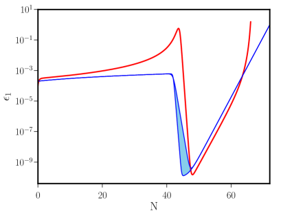
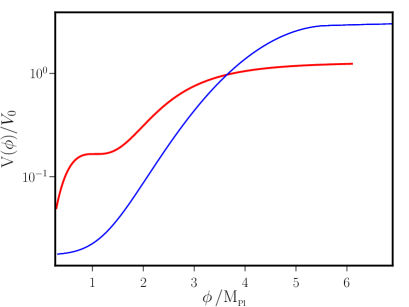
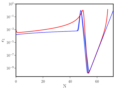
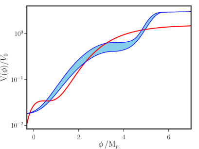
The parameters we have worked with in the case of the reconstructed scenario RS1 are as follows: $\epsilon_{1a}=10^{-4}$, $\epsilon_{2a}=5\times 10^{-2}$, $\epsilon_{1b}=10^{-10}$, $N_{1}=42$, $N_{2}=72$ and $\Delta N_{2}=1.1$. We have varied the parameter $\Delta N_{1}$ over the range $(0.3345,0.7)$ to obtain the bands of $\epsilon_{1}$ and the corresponding potential in the figure. Similarly, in the case of RS2, the parameters we have chosen to work with are as follows: $\epsilon_{1a}=8\times 10^{-5}$, $\epsilon_{2a}=6.25\times 10^{-2}$, $\epsilon_{1b}=10^{-10}$, $N_{1}=48$, $N_{2}=72$ and $\Delta N_{2}=0.8$. The parameter $\Delta N_{1}$ has been varied over the range $(0.3847,0.5)$ to arrive at the bands of $\epsilon_{1}$ and the corresponding potential. We should note that the band describing the potential is more pronounced in the case of RS2 than in RS1. The choices for $\epsilon_{1a}$ and $\epsilon_{2a}$ have been made so that the resulting power spectra are consistent with the Planck constraints on the scalar spectral index $n_{{}_{\mathrm{S}}}$ and the tensor-to-scalar ratio $r$ at the pivot scale that we mentioned earlier. For comparison, in the figure, we have also included the behavior of the first slow parameter as well as the form of the potential in the models USR2 and PI3. It should be clear that, for suitable values of the parameters, our functional forms for $\epsilon_{1}(N)$ closely mimic the corresponding behavior in these models. Moreover, from the parametric forms of $V(\phi)$ constructed numerically, we have been able to determine if the reconstructed potentials in the cases of RS1 and RS2 contain a point of inflection. At an accuracy of $0.1\%$, we find that the reconstructed potentials indeed contain an inflection point.

With the background quantities at hand, it is straightforward to compute the power spectra by integrating the differential equations (9) for the curvature and the tensor perturbations. In figure 6, we have plotted the power spectra that arise in the scenarios RS1 and RS2.

Figure 6: The scalar (in solid blue) and tensor power spectra (in dashed blue) resulting from the scenarios RS1 (on top) and RS2 (at the bottom) have been plotted over a wide range of wave numbers. For comparison, we have also plotted the scalar (in solid red) and tensor (in dashed red) power spectra that arise in the cases of USR2 (on top) and in PI3 (at the bottom). In the cases of RS1 and RS2 (plotted in blue), we have chosen the parameters so that the peak in the scalar power spectra roughly coincides with the peaks in the models of USR2 and PI3 (plotted in red), respectively. In addition, we have plotted the spectra arising in RS1 and RS2 for two other values of the parameter $N_{1}$ to produce peaks in the scalar power at smaller wave numbers (in green and orange). Actually, we have plotted the spectra in RS1 and RS2 as bands (in blue, green and orange) corresponding to a small range of the parameter $\Delta N_{1}$ [cf. eqs. (14)].

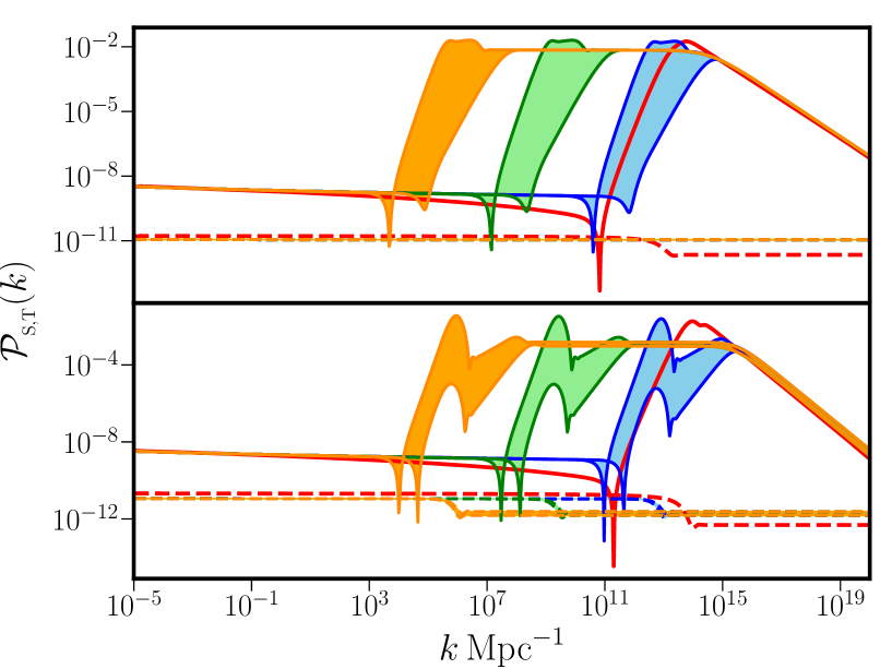
We have also compared the power spectra in these cases with the spectra in USR2 and PI3. It is clear that, while the scalar power spectra from the reconstructed potentials are indeed very similar to the power spectra from USR2 and PI3, the corresponding tensor power spectra exhibit some differences. Since we shall be focusing on the observational imprints of the scalar perturbations generated during inflation, we shall ignore these differences for now. We shall make a few clarifying remarks regarding this point in the concluding section.

Earlier, we had emphasized the point that the models USR2 and PI3 are highly fine-tuned and that it is difficult to move the locations of the peaks in the scalar power spectra substantially without either considerably affecting the duration of inflation or the spectra over the CMB scales. In contrast, because of the presence of the additional parameters, the scenarios RS1 and RS2 are easier to tune and, as a result, we find that we can shift the location of the peak as well as broaden its width. In figure 6, apart from the spectra in RS1 and RS2 which closely mimic the scalar spectra that arise in USR2 and PI3, we have plotted the power spectra for two other sets of parameters which lead to peaks at different locations and also exhibit a broader peak. These spectra have been achieved by choosing different values for the parameter $N_{1}$, while keeping the other parameters fixed at the values mentioned earlier. To arrive at the spectra with the broader peaks in figure 6, we have set $N_{1}=34$ and $26$ in the case of RS1 and $N_{1}=40$ and $32$ in the case of RS2. We should mention that a smaller choice of $N_{1}$ leads to a peak at a smaller wave number. Moreover, the bands associated with these two spectra correspond to the variation of the parameter $\Delta N_{1}$ over the domain we had mentioned before.

In the next two sections, we shall study the imprints of the various power spectra on the formation of PBHs and the generation of secondary GWs.

V Formation of PBHs

Let us begin by recalling a few essentials. Scales with wave numbers greater than $k\simeq 10^{-2}\,\mathrm{Mpc}^{-1}$ renter the Hubble radius during the radiation dominated epoch. When these modes reenter the Hubble radius, the perturbations in the matter density at the corresponding scales collapse to form structures. We shall assume that the density contrast in matter characterized by the quantity $\delta$ is a Gaussian random variable described by the probability density

$${\cal P}(\delta)=\frac{1}{\sqrt{2\,\pi\,\sigma^{2}}}\;\mathrm{exp}{\left(-\frac{\delta^{2}}{2\,\sigma^{2}}\right)},$$ (17)

where $\sigma^{2}$ is the variance of the spatial density fluctuations. Let us assume that perturbations with a density contrast beyond a certain threshold, say, $\delta_{\mathrm{c}}$, are responsible for the formation of PBHs. In such a case, the fraction, say, $\beta$, of the density fluctuations that collapse to form PBHs is described by the integral (in this context, see the reviews [18, 19, 20, 21])

$$\beta=\int^{1}_{{}_{\delta_{\mathrm{c}}}}{\mathrm{d}}\delta\,{\mathcal{P}}(\delta)\simeq\frac{1}{2}\,\left[1-\mathrm{erf}\left(\frac{\delta_{\mathrm{c}}}{\sqrt{2\,\sigma^{2}}}\right)\right],$$ (18)

where $\mathrm{erf}(z)$ denotes the error function. Note that the lower limit of the above integral is the threshold value of the density contrast beyond which matter is expected to collapse to form PBHs. We should clarify here that the value of $\delta_{\mathrm{c}}$ is not unique and it is expected to depend on the amplitude of the perturbation at a given scale (see refs. [16, 88]; in this context, also see the recent discussions [20, 89, 90, 91, 92, 93]). The choice of $\delta_{\mathrm{c}}$ becomes important for the reason that the extent of PBHs formed is exponentially sensitive to its value. In order to calculate the extent of PBHs formed, we shall work with the following values of $\delta_{\mathrm{c}}$: $1/3$, $0.35$ and $0.4$.

During the radiation dominated epoch, the matter power spectrum $P_{\delta}(k)$ and the inflationary scalar power spectrum $\mathcal{P}_{{}_{\mathrm{S}}}(k)$ are related through the expression

$$P_{\delta}(k)=\frac{16}{81}\,\left(\frac{k}{aH}\right)^{4}\,\mathcal{P}_{{}_{\mathrm{S}}}(k).$$ (19)

The variance in the spatial density fluctuations $\sigma^{2}$, which determines the fraction $\beta$ of PBHs formed [cf. eq. (18)], can be expressed as an integral over the matter power spectrum $P_{\delta}(k)$. In order to introduce a length scale, say, $R$, the variance is smoothened over the scale with the aid of a window function $W(k\,R)$. The variance $\sigma^{2}(R)$ can then be written as

$$\sigma^{2}(R)=\int_{0}^{\infty}\frac{{\mathrm{d}}k}{k}\,P_{\delta}(k)\,W^{2}(k\,R),$$ (20)

and we shall work with a Gaussian window function of the form $W(k\,R)=\mathrm{e}^{-(k^{2}\,R^{2})/2}$.

There remains the task of relating the scale $R$ to the mass, say, $M$, of the PBHs formed. Let $M_{{}_{\mathrm{H}}}$ denote the mass within the Hubble radius $H^{-1}$ at a given time. It is reasonable to suppose that a certain fraction of the total mass within the Hubble radius, say, $M=\gamma\,M_{\mathrm{H}}$, goes on to form PBHs when a mode with wave number $k$ reenters the Hubble radius. The quantity $\gamma$ that has been introduced reflects the efficiency of the collapse. In the absence of any other scale, it seems natural to choose $k=R^{-1}$, and make use of the fact that $k=a\,H$ when the modes reenter the Hubble radius, to finally obtain the relation between $R$ and $M$. One can show that $R$ and $M$ are related as follows:

$$R=\frac{2^{1/4}}{\gamma^{1/2}}\,\left(\frac{g_{\ast,k}}{g_{\ast,\mathrm{eq}}}\right)^{1/12}\,\left(\frac{1}{k_{\mathrm{eq}}}\right)\,\left(\frac{M}{M_{\mathrm{eq}}}\right)^{1/2},$$ (21)

where $k_{\mathrm{eq}}$ is the wave number that reenters the Hubble radius at the epoch of radiation-matter equality, and $M_{\mathrm{eq}}$ denotes the mass within the Hubble radius at equality. Also, the quantities $g_{\ast,k}$ and $g_{\ast,\mathrm{eq}}$ represent the number of relativistic degrees of freedom at the times of PBH formation and radiation-matter equality, respectively. It can be easily determined that $M_{\mathrm{eq}}=5.83\times 10^{47}\,\mathrm{kg}$, so that we can express the above relation between $R$ and $M$ in terms of the solar mass $M_{\odot}$ as follows:

$$R=4.72\times 10^{-7}\,\left(\frac{\gamma}{0.2}\right)^{-1/2}\,\left(\frac{g_{\ast,k}}{g_{\ast,\mathrm{eq}}}\right)^{1/12}\,\left(\frac{M}{M_{\odot}}\right)^{1/2}\,\mathrm{Mpc}.$$ (22)

On using the above arguments, we can arrive at the fraction of PBHs, say, $f_{{}_{\mathrm{PBH}}}$, that contribute to the dark matter density today. The quantity $f_{{}_{\mathrm{PBH}}}(M)$ can be expressed as

$$f_{{}_{\mathrm{PBH}}}(M)=2^{1/4}\;\gamma^{3/2}\,\beta(M)\,\left(\frac{\Omega_{\mathrm{m}}\,h^{2}}{\Omega_{\mathrm{c}}\,h^{2}}\right)\,\left(\frac{g_{\ast,k}}{g_{\ast,\mathrm{eq}}}\right)^{-1/4}\,\left(\frac{M}{M_{\mathrm{eq}}}\right)^{-1/2},$$ (23)

where $\Omega_{\mathrm{m}}$ and $\Omega_{\mathrm{c}}$ are the dimensionless parameters describing the matter and cold matter densities, with the Hubble parameter, as usual, expressed as $H_{0}=100\,h\,\mathrm{km}\,\mathrm{sec}^{-1}\,\mathrm{Mpc}^{-1}$. In our calculations, we shall choose $\gamma=0.2$, $g_{\ast,k}=106.75$ and $g_{\ast,\mathrm{eq}}=3.36$ and set $\Omega_{\mathrm{m}}\,h^{2}=0.14$, $\Omega_{\mathrm{c}}\,h^{2}=0.12$, with the last two being the best fit values from the recent Planck data [94, 95]. On substituting these values, one can arrive at the following expression for $f_{{}_{\mathrm{PBH}}}(M)$:

$$f_{{}_{\mathrm{PBH}}}(M)=\left(\frac{\gamma}{0.2}\right)^{3/2}\,\left(\frac{\beta(M)}{1.46\times 10^{-8}}\right)\,\left(\frac{g_{\ast,k}}{g_{\ast,\mathrm{eq}}}\right)^{-1/4}\,\left(\frac{M}{M_{\odot}}\right)^{-1/2}.$$ (24)

Given a primordial power spectrum $\mathcal{P}_{{}_{\mathrm{S}}}(k)$, we can utilize the relations (19) and (20) to arrive at the quantity $\sigma^{2}(R)$. Then, using the relation (21), we can determine $\sigma^{2}$ as a function of $M$ and utilize the result (18) to obtain $\beta(M)$. With $\beta(M)$ at hand, we can use the relation (24) to finally arrive at $f_{{}_{\mathrm{PBH}}}(M)$ for a given inflationary scalar power spectrum. In figure 7, we have plotted $f_{{}_{\mathrm{PBH}}}(M)$ for the models of USR2, PI3, RS1, and RS2.

Figure 7: The fraction of PBHs contributing to the dark matter density today $f_{{}_{\mathrm{PBH}}}$ has been plotted for the various models and scenarios of interest, viz. USR2 and RS1 (on top, in red and blue) and PI3 and RS2 (at the bottom, in red and blue). We have plotted the quantity $f_{{}_{\mathrm{PBH}}}$ for the following three values of $\delta_{\mathrm{c}}$: $1/3$ (as solid curves) and $0.35$ (as dashed curves) and $0.4$ (as dotted curves). In the cases of RS1 and RS2, apart from the original choices of parameters that led to scalar spectra that closely matched the spectra in USR2 and PI3, we have plotted the quantity $f_{{}_{\mathrm{PBH}}}$ for spectra which had exhibited broader peaks starting at smaller wave numbers (cf. figure 6). As in the previous figure, in the cases of RS1 and RS2, we have plotted bands corresponding to a range of the parameter $\Delta N_{1}$. We have also indicated the latest direct (in different colors) and indirect (in gray) constraints on $f_{{}_{\mathrm{PBH}}}$ from a variety of observations. We should mention here that the indirect constraints depend on additional assumptions. Evidently, for the parameters of the potentials we have been working with, USR2 leads to a larger formation of PBHs than PI3. Moreover, note that the existing observational constraints already limit the parameter $\Delta N_{1}$ in the reconstructions RS1 and RS2.

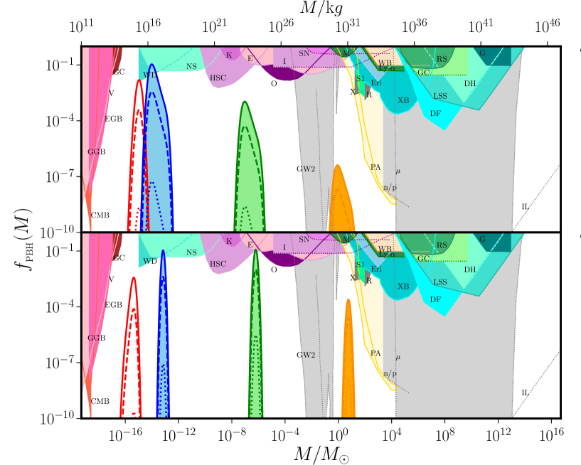
In the figure, we have also indicated the constraints from the various observations such as constraints from gravitational lensing [96, 97], constraints due to the limits on extragalactic background photons from PBH evaporation [17], constraints from microlensing searches by Kepler [98], MACHO [99], EROS [100] and OGLE [101], constraints from the large scale structure [17], constraints from the CMB anisotropies due to accretion onto PBHs (FIRAS and WMAP3) [102] and, finally, constraints from the dynamics of ultra-faint dwarf galaxies [103]. (For the latest and comprehensive list of these constraints and a detailed discussion, see refs. [104, 105]. For related discussions in these contexts, also see refs. [106, 107, 108, 109].) We find that, in the cases of USR2 and RS1, where the location of the peaks in the scalar power spectra approximately match, the maximum values of $f_{{}_{\mathrm{PBH}}}$ achieved are $1.5\times 10^{-2}$ and $0.10$, respectively. For the models PI3 and RS2, when the peaks are located at roughly the same wave number, we similarly obtain $f_{{}_{\mathrm{PBH}}}$ to be $3\times 10^{-3}$ and $0.11$ at their respective maxima. In these cases, the maxmima in $f_{{}_{\mathrm{PBH}}}(M)$ are located over the domain $M\simeq 10^{-16}$–$10^{-12}\,M_{\odot}$. For peaks in the scalar power spectra that occur at smaller wave numbers in the cases of RS1 and RS2, as expected, the locations of the maxima in $f_{{}_{\mathrm{PBH}}}(M)$ shift towards larger masses of PBHs. Interestingly, for the power spectra in RS1 and RS2 which exhibit a broad peak beginning at $k\simeq\,10^{6}\,\mathrm{Mpc}^{-1}$, there arise maxima in $f_{{}_{\mathrm{PBH}}}$ at tens of solar masses. However, the corresponding maximum value of $f_{{}_{\mathrm{PBH}}}$ at $M\simeq 10\,M_{\odot}$ is a few orders of magnitude smaller than the maximum values we discussed above at smaller masses. This arises despite the fact the amplitude of the scalar power spectra at their peak is the same in all these cases. We believe that this result can be attributed to the dependence of $f_{{}_{\mathrm{PBH}}}$ on $M$ as $M^{-1/2}$ [cf. eq. (24)]. We should point out here that the shaded bands corresponding to RS1 and RS2 in figure 7 indicate the range of $f_{{}_{\mathrm{PBH}}}$ that can be generated by varying the parameter $\Delta N_{1}$ in the functional forms of $\epsilon_{1}(N)$ [cf. eqs. (14)]. The intersection of the shaded bands with the constraints readily translate to the limits on this parameter in our reconstructions RS1 and RS2. We find that a smaller $\Delta N_{1}$ leads to a steeper growth of power and hence to a higher fraction of PBHs. Therefore, for a fixed set of values for the other parameters, the constraints essentially restrict the rapidity of the transition of inflation from slow roll to ultra slow roll epoch in our reconstructions.

VI Generation of secondary GWs

In this section, we shall calculate the secondary power and bispectrum of GWs induced by the scalar perturbations at the second order.

VI.1 The secondary tensor power spectrum

Earlier, we had described the scalar and tensor perturbations at first order in terms of the curvature perturbation ${\mathcal{R}}$ and the quantity $\gamma_{ij}$ (cf. subsection III.1). It is well known that, at the linear order, the scalar and tensor perturbations evolve independently, with their evolution being governed by the corresponding equations of motion, viz. eqs. (9). However, one finds that, at the second order, the tensor perturbations are sourced by quadratic terms involving the first order scalar perturbations (for early discussions in this context, see for instance, refs. [38, 39, 40, 41]). These contributions due to the scalar perturbations become important particularly when the amplitude of the scalar power spectrum is boosted over small scales such as in the situations leading to enhanced formation of PBHs. In this subsection, we shall calculate the dimensionless density parameter associated with the GWs, say, $\Omega_{{}_{\mathrm{GW}}}$, generated due to the scalar perturbations in the different models and scenarios of interest.

Let us begin by outlining the primary steps towards the calculation of $\Omega_{{}_{\mathrm{GW}}}(f)$, where $f$ is the frequency associated with the wave number $k$. We shall start with the following perturbed metric:

$${\mathrm{d}}s^{2}=a^{2}(\eta)\,\left\{-\left(1+2\,\Phi\right)\,{\mathrm{d}}\eta^{2}+\left[\left(1-2\,\Psi\right)\,\delta_{ij}+\frac{1}{2}\,h_{ij}\right]\,{\mathrm{d}}x^{i}{\mathrm{d}}x^{j}\right\},$$ (25)

where $\Phi$ and $\Psi$ are the Bardeen potentials describing the scalar perturbations at the first order, while the quantity $h_{ij}$ represents the second order tensor perturbations. We should clarify that we have denoted the second order tensor perturbation as $h_{ij}$ in order to distinguish them from the first order tensor perturbations $\gamma_{ij}$ which we had introduced earlier. The transverse and traceless nature of the tensor perturbations implies that ${\partial}^{i}\,h_{ij}=0$ and $h^{i}_{i}=0$. In our discussion below, we shall assume that anisotropic stresses are absent so that $\Phi=\Psi$.

The tensor perturbations $h_{ij}$ can be decomposed in terms of the Fourier modes, say, $h_{\bm{k}}$, as

$$h_{ij}(\eta,{\bm{x}})=\int\frac{{\mathrm{d}}^{3}{\bm{k}}}{(2\,\pi)^{3/2}}\,\left[e_{ij}^{+}({\bm{k}})\,h_{{\bm{k}}}^{+}(\eta)+e_{ij}^{\times}({\bm{k}})\,h_{{\bm{k}}}^{\times}(\eta)\right]\,{\rm e}^{i\,{\bm{k}}\cdot{\bm{x}}},$$ (26)

where $e_{ij}^{+}({\bm{k}})$ and $e_{ij}^{\times}({\bm{k}})$ denote the polarization tensors which have non-zero components in the plane perpendicular to the direction of propagation, viz. $\hat{{\bm{k}}}$. The polarization tensors $e_{ij}^{+}({\bm{k}})$ and $e_{ij}^{\times}({\bm{k}})$ can be expressed in terms of the set of orthogonal unit vectors $(e({\bm{k}}),{\bar{e}}({\bm{k}}),\hat{{\bm{k}}})$ in the following manner (see, for instance, the review [110]):

$$e_{ij}^{+}({\bm{k}}) = \frac{1}{\sqrt{2}}\,\left[e_{i}({\bm{k}})\,e_{j}({\bm{k}})-{\bar{e}}_{i}({\bm{k}})\,{\bar{e}}_{j}({\bm{k}})\right],$$ (27a)

$$e_{ij}^{\times}({\bm{k}}) = \frac{1}{\sqrt{2}}\,\left[e_{i}({\bm{k}})\,{\bar{e}}_{j}({\bm{k}})+{\bar{e}}_{i}({\bm{k}})\,e_{j}({\bm{k}})\right].$$ (27b)

The orthonormal nature of the vectors $e({\bm{k}})$ and ${\bar{e}}({\bm{k}})$ lead to the normalization condition: $e_{ij}^{\lambda}({\bm{k}})\,e^{\lambda^{\prime},ij}({\bm{k}})=\delta^{\lambda\lambda^{\prime}}$, where $\lambda$ and $\lambda^{\prime}$ can be either $+$ or $\times$.

The equation of motion governing the Fourier modes $h_{\bm{k}}$ can be arrived at using the second order Einstein equations describing the tensor perturbation $h_{ij}$ and the Bardeen equation describing the scalar perturbation $\Psi$ at the first order (see, for example, refs. [38, 39]; for recent discussions, see refs. [111, 112, 113, 43]). One finds that the equation governing $h_{\bm{k}}$ can be written as

$${h_{\bm{k}}^{\lambda}}^{\prime\prime}+2\,\mathcal{H}\,{h_{\bm{k}}^{\lambda}}^{\prime}+k^{2}\,h_{\bm{k}}^{\lambda}=S_{\bm{k}}^{\lambda}$$ (28)

with the source term $S_{\bm{k}}^{\lambda}$ being given by

$$S_{\bm{k}}^{\lambda}(\eta) = 4\,\int\frac{{\mathrm{d}}^{3}{\bm{p}}}{(2\,\pi)^{3/2}}\,e^{\lambda}({\bm{k}},{\bm{p}})\,\Biggl{\{}2\,\Psi_{\bm{p}}(\eta)\,\Psi_{{\bm{k}}-{\bm{p}}}(\eta)$$ (29)

$$+\,\frac{4}{3\,(1+w)\,{\mathcal{H}}^{2}\,}\,\left[\Psi_{\bm{p}}^{\prime}(\eta)+{\cal H}\,\Psi_{\bm{p}}(\eta)\right]\,\left[\Psi_{{\bm{k}}-{\bm{p}}}^{\prime}(\eta)+{\cal H}\,\Psi_{{\bm{k}}-{\bm{p}}}(\eta)\right]\,\Biggr{\}},$$

where, evidently, $\Psi_{\bm{k}}$ represents the Fourier modes of the Bardeen potential, while ${\cal H}$ and $w$ denote the conformal Hubble parameter and the equation of state parameter describing the universe at the conformal time $\eta$. Also, for convenience, we have defined the quantity $e^{\lambda}({\bm{k}},{\bm{p}})=e^{\lambda}_{ij}({\bm{k}})\,p^{i}\,p^{j}$. While discussing the formation of PBHs earlier, we had assumed that the scales of our interest reenter the Hubble radius during the epoch of radiation domination. In such a case, we have $w=1/3$ and ${\cal H}=1/\eta$. Moreover, during radiation domination, it is well known that we can express the Fourier modes $\Psi_{\bm{k}}$ of the Bardeen potential in terms of the inflationary Fourier modes ${\mathcal{R}}_{\bm{k}}$ of the curvature perturbations generated during inflation through the relation

$$\Psi_{\bm{k}}(\eta)=\frac{2}{3}\,{\mathcal{T}}(k\,\eta)\,{\mathcal{R}}_{\bm{k}},$$ (30)

where ${\mathcal{T}}(k\,\eta)$ is the transfer function given by

$${\mathcal{T}}(k\,\eta)=\frac{9}{\left(k\,\eta\right)^{2}}\,\left[\frac{{\rm sin}\left(k\,\eta/\sqrt{3}\right)}{k\,\eta/\sqrt{3}}-{\rm cos}\left(k\,\eta/\sqrt{3}\right)\right].$$ (31)

Utilizing the Green’s function corresponding to the tensor modes during radiation domination, we can express the inhomogeneous contribution to $h_{\bm{k}}^{\lambda}$ as [43]

$$h_{\bm{k}}^{\lambda}(\eta) = \frac{4}{9\,k^{3}\,\eta}\,\int\frac{{\mathrm{d}}^{3}{\bm{p}}}{(2\,\pi)^{3/2}}\,e^{\lambda}({\bm{k}},{\bm{p}})\,{\mathcal{R}}_{\bm{k}}\,{\mathcal{R}}_{{\bm{k}}-{\bm{p}}}\,\left[{\mathcal{I}}_{c}\left(\frac{p}{k},\frac{|{\bm{k}}-{\bm{p}}|}{k}\right)\,{\rm cos}\left(k\,\eta\right)+{\mathcal{I}}_{s}\left(\frac{p}{k},\frac{|{\bm{k}}-{\bm{p}}|}{k}\right)\,{\rm sin}\left(k\,\eta\right)\right],$$ (32)

where the quantities ${\mathcal{I}}_{c}(v,u)$ and ${\mathcal{I}}_{s}(v,u)$ are described by the integrals

$${\mathcal{I}}_{c}(v,u) = -4\,\int_{0}^{\infty}\,{\mathrm{d}}\tau\,\tau\,{\rm sin}\,\tau\,\biggl{\{}2\,{\mathcal{T}}(v\,\tau)\,{\mathcal{T}}(u\,\tau)+\left[{\mathcal{T}}(v\,\tau)+v\,\tau\,{\mathcal{T}}_{v\tau}(v\,\tau)\right]\,\left[{\mathcal{T}}(u\,\tau)+u\,\tau\,{\mathcal{T}}_{u\tau}(u\,\tau)\right]\biggr{\}},$$ (33a)

$${\mathcal{I}}_{s}(v,u) = 4\,\int_{0}^{\infty}\,{\mathrm{d}}\tau\,\tau\,{\rm cos}\,\tau\,\biggl{\{}2\,{\mathcal{T}}(v\,\tau)\,{\mathcal{T}}(u\,\tau)+\left[{\mathcal{T}}(v\,\tau)+v\,\tau\,{\mathcal{T}}_{v\tau}(v\,\tau)\right]\,\left[{\mathcal{T}}(u\,\tau)+u\,\tau\,{\mathcal{T}}_{u\tau}(u\,\tau)\right]\biggr{\}},$$ (33b)

with ${\mathcal{T}}_{z}={\mathrm{d}}{\mathcal{T}}/{\mathrm{d}}z$. The above integrals can be carried out analytically and they are given by

$${\mathcal{I}}_{c}(v,u) = -\frac{27\,\pi}{4\,v^{3}\,u^{3}}\,\Theta\left(v+u-\sqrt{3}\right)\,(v^{2}+u^{2}-3)^{2},$$ (34a)

$${\mathcal{I}}_{s}(v,u) = -\frac{27}{4\,v^{3}\,u^{3}}\,(v^{2}+u^{2}-3)\,\left[4\,v\,u+(v^{2}+u^{2}-3)\;{\rm log}\,\biggl{|}\frac{3-(v-u)^{2}}{3-(v+u)^{2}}\biggr{|}\right],\qquad$$ (34b)

where $\Theta(z)$ denotes the theta function. It is useful to note that ${\mathcal{I}}_{c,s}(v,u)={\mathcal{I}}_{c,s}(u,v)$.

The power spectrum of the secondary GWs, say, $\mathcal{P}_{h}(k,\eta)$, generated due to the second order scalar perturbations can be defined as follows:

$$\langle h_{{\bm{k}}}^{\lambda}(\eta)\,h_{{\bm{k}}^{\prime}}^{\lambda^{\prime}}(\eta)\rangle=\frac{2\,\pi^{2}}{k^{3}}\,{\mathcal{P}}_{h}(k,\eta)\,\delta^{(3)}({\bm{k}}+{\bm{k}}^{\prime})\,\delta^{\lambda\lambda^{\prime}}.$$ (35)

Note that $h_{\bm{k}}^{\lambda}$ involves products of the Fourier modes ${\mathcal{R}}_{\bm{k}}$ and ${\mathcal{R}}_{{\bm{k}}-{\bm{p}}}$ of the curvature perturbations generated during inflation [cf. eq. (32)]. Evidently, the power spectrum $\mathcal{P}_{h}(k)$ of the secondary GWs will involve products of four such variables. Since, the quantity ${\mathcal{R}}_{\bm{k}}$ is a Gaussian random variable, we can express the four-point function in terms of the two-point functions or, equivalently, the inflationary scalar power spectrum $\mathcal{P}_{{}_{\mathrm{S}}}(k)$ [cf. eq. (10a)] as

$$\mathcal{P}_{h}(k,\eta) = \frac{4}{81\,k^{2}\,\eta^{2}}\int_{0}^{\infty}{\mathrm{d}}v\,\int_{|1-v|}^{1+v}{\mathrm{d}}u\,\left[\frac{4\,v^{2}-(1+v^{2}-u^{2})^{2}}{4\,u\,v}\right]^{2}\,\mathcal{P}_{{}_{\mathrm{S}}}(k\,v)\,\mathcal{P}_{{}_{\mathrm{S}}}(k\,u)$$ (36)

$$\times\,\left[{\mathcal{I}}_{c}(u,v)\,{\rm cos}\left(k\,\eta\right)+{\mathcal{I}}_{s}(u,v)\,{\rm sin}\left(k\,\eta\right)\right]^{2}.$$

We shall now choose to average $\mathcal{P}_{h}(k,\eta)$ over small time scales so that the trigonometric functions in the above expressions are replaced by their average over a time period. In such a case, only the overall time dependence remains, leading to [42, 43]

$$\overline{\mathcal{P}_{h}(k,\eta)} = \frac{2}{81\,k^{2}\,\eta^{2}}\int_{0}^{\infty}{\mathrm{d}}v\,\int_{|1-v|}^{1+v}{\mathrm{d}}u\,\left[\frac{4\,v^{2}-(1+v^{2}-u^{2})^{2}}{4\,u\,v}\right]^{2}\,\mathcal{P}_{{}_{\mathrm{S}}}(k\,v)\,\mathcal{P}_{{}_{\mathrm{S}}}(k\,u)$$ (37)

$$\times\,\left[{\mathcal{I}}_{c}^{2}(u,v)+{\mathcal{I}}_{s}^{2}(u,v)\right],$$

where the line over $\mathcal{P}_{h}(k,\eta)$ implies that we have averaged over small time scales. The energy density of GWs associated with a Fourier mode corresponding to the wave number $k$ at a time $\eta$ is given by [110]

$$\rho_{{}_{\mathrm{GW}}}(k,\eta)=\frac{M_{{}_{\mathrm{Pl}}}^{2}}{8}\,\left(\frac{k}{a}\right)^{2}\,\overline{\mathcal{P}_{h}(k,\eta)}.$$ (38)

The corresponding dimensionless density parameter $\Omega_{{}_{\mathrm{GW}}}(k,\eta)$ can be defined in terms of the critical density $\rho_{\mathrm{cr}}(\eta)$ as [43]

$$\Omega_{{}_{\mathrm{GW}}}(k,\eta)=\frac{\rho_{{}_{\mathrm{GW}}}(k,\eta)}{\rho_{\mathrm{cr}}(\eta)}=\frac{1}{24}\,\left(\frac{k}{{\mathcal{H}}}\right)^{2}\overline{\mathcal{P}_{h}(k,\eta)}.$$ (39)

Note that the dimensionless density parameter $\Omega_{{}_{\mathrm{GW}}}(k,\eta)$ above has been evaluated during the radiation dominated epoch. Once the modes are inside the Hubble radius, the energy density of GWs decay just as the energy density of radiation does. Upon utilizing this point, we can express $\Omega_{{}_{\mathrm{GW}}}(k)$ today in terms of the above $\Omega_{{}_{\mathrm{GW}}}(k,\eta)$ as follows:

$$h^{2}\,\Omega_{{}_{\mathrm{GW}}}(k) = \left(\frac{g_{\ast,k}}{g_{\ast,0}}\right)^{-1/3}\,\Omega_{\mathrm{r}}\,h^{2}\;\Omega_{{}_{\mathrm{GW}}}(k,\eta)$$ (40)

$$\simeq 1.38\times 10^{-5}\,\left(\frac{g_{\ast,k}}{106.75}\right)^{-1/3}\,\left(\frac{\Omega_{r}\,h^{2}}{4.16\times 10^{-5}}\right)\,\Omega_{{}_{\mathrm{GW}}}(k,\eta),$$

where $\Omega_{\mathrm{r}}$ and $g_{\ast,0}$ denote the dimensionless energy density of radiation and the number of relativistic degrees of freedom today. We should point out here that, since $\mathcal{H}\propto\eta^{-1}$ during radiation domination and $\mathcal{P}_{h}(k,\eta)\propto\eta^{-2}$, the quantity $\Omega_{{}_{\mathrm{GW}}}(k,\eta)$ in the expression (39) is actually independent of time. Moreover, the observable parameter today is usually expressed as a function of the frequency, say, $f$, which is related to the wave number $k$ as

$$f=\frac{k}{2\,\pi}=1.55\times 10^{-15}\,\left(\frac{k}{1\,\mathrm{Mpc}^{-1}}\right)\,\mathrm{Hz}.$$ (41)

In figure 8, we have plotted the quantity $\Omega_{{}_{\mathrm{GW}}}(f)$ arising in the models USR2 and PI3 as well as the reconstructed scenarios RS1 and RS2.

Figure 8: The dimensionless density parameter $\Omega_{{}_{\mathrm{GW}}}$ associated with the secondary GWs generated in the models and reconstructed scenarios of USR2 and RS1 (in red and blue, on top) as well as PI3 and RS2 (in red and blue, at the bottom) have been plotted as a function of the frequency $f$. We have also plotted the $\Omega_{{}_{\mathrm{GW}}}$ produced by the scenarios RS1 and RS2 with broader peaks beginning at smaller wave numbers (in green and orange). The bands of spectra, as with the previous figures, correspond to variation of the parameter $\Delta N_{1}$ for a given $N_{1}$. Moreover, we have included the sensitivity curves of various existing and upcoming observational probes of GWs (as shaded regions, in the top part of the panels). Clearly, it should be possible to detect the GWs generated in the models and scenarios of our interest by some of the forthcoming observatories.

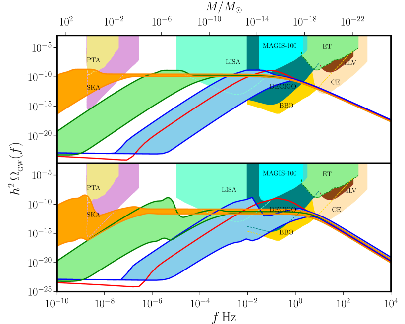
In the figure, we have also included the sensitivity curves associated with the various current and forthcoming observatories, viz. PTA and the Square Kilometre Array (SKA) [114], LISA [111], MAGIS-100 [115, 43], BBO [51, 52, 53], DECIGO [54, 55], ET [57], advanced LIGO $+$ Virgo [45, 116] and CE [117]. (For a summary of the sensitivity curves and their updated versions, see ref. [114] and the associated web-page.) We should mention here that the estimated sensitivity curves have been arrived at assuming a power law spectrum (the so-called ‘power-law integrated curves’) over the bands of interest. These sensitivities are expected to be achieved by integrating over frequency in addition to integrating over time [118, 119]. It should be evident from the figure that the strength of the GWs generated in the models and scenarios we have examined here is significant enough to be detectable by one or more of these observatories. Recall that, spectra arising in the scenarios RS1 and RS2 with broad peaks starting from a wave number of about $10^{6}\,\mathrm{Mpc}^{-1}$ had led to PBHs with tens of solar masses. It should be clear from figure 8 that the constraints from PTA on $\Omega_{{}_{\mathrm{GW}}}$ already rule out such spectra for certain values of $\Delta N_{1}$.

VI.2 The secondary tensor bispectrum

In this section, we shall evaluate the secondary tensor bispectrum generated in the inflationary models and scenarios of our interest. The secondary tensor bispectrum, say, ${\mathcal{B}}^{\lambda_{1}\lambda_{2}\lambda_{3}}_{h}({\bm{k}}_{1},{\bm{k}}_{2},{\bm{k}}_{3})$ is defined as

$$\left\langle h_{{\bm{k}}_{1}}^{\lambda_{1}}(\eta)\,h_{{\bm{k}}_{2}}^{\lambda_{2}}(\eta)\,h_{{\bm{k}}_{3}}^{\lambda_{3}}(\eta)\right\rangle=(2\,\pi)^{3}\,{\mathcal{B}}_{h}^{\lambda_{1}\lambda_{2}\lambda_{3}}({\bm{k}}_{1},{\bm{k}}_{2},{\bm{k}}_{3},\eta)\,\delta^{(3)}({\bm{k}}_{1}+{\bm{k}}_{2}+{\bm{k}}_{3}).$$ (42)

We can evaluate the above tensor bispectrum during the radiation dominated era by using the expression (32) for $h^{\lambda}_{{\bm{k}}}(\eta)$. As we had discussed, $h^{\lambda}_{{\bm{k}}}(\eta)$ is quadratic in the Gaussian variables ${\mathcal{R}}_{\bm{k}}$. Therefore, obviously, the bispectrum ${\mathcal{B}}_{h}^{\lambda_{1}\lambda_{2}\lambda_{3}}({\bm{k}}_{1},{\bm{k}}_{2},{\bm{k}}_{3},\eta)$ will involve six of these variables. Upon utilizing Wick’s theorem applicable to Gaussian random variables, one can show that the tensor bispectrum consists of eight terms all of which lead to the same contribution [113, 43]. For convenience, we shall define $G_{h}^{\lambda_{1}\lambda_{2}\lambda_{3}}({\bm{k}}_{1},{\bm{k}}_{2},{\bm{k}}_{3},\eta)=(2\,\pi)^{-9/2}\;{\mathcal{B}}_{h}^{\lambda_{1}\lambda_{2}\lambda_{3}}({\bm{k}}_{1},{\bm{k}}_{2},{\bm{k}}_{3},\eta)$ and hereafter refer to $G_{h}^{\lambda_{1}\lambda_{2}\lambda_{3}}({\bm{k}}_{1},{\bm{k}}_{2},{\bm{k}}_{3},\eta)$ as the secondary tensor bispectrum. We find that the secondary tensor bispectrum can be expressed as

$$G_{h}^{\lambda_{1}\lambda_{2}\lambda_{3}}({\bm{k}}_{1},{\bm{k}}_{2},{\bm{k}}_{3},\eta) = \left(\frac{8\,\pi}{9}\right)^{3}\,\frac{1}{(k_{1}\,k_{2}\,k_{3}\,\eta)^{3}}$$ (43)

$$\times\,\int{\mathrm{d}}^{3}{\bm{p}}_{1}\,e^{\lambda_{1}}({\bm{k}}_{1},{\bm{p}}_{1})\,e^{\lambda_{2}}({\bm{k}}_{2},{\bm{p}}_{2})\,e^{\lambda_{3}}({\bm{k}}_{3},{\bm{p}}_{3})\,\frac{\mathcal{P}_{{}_{\mathrm{S}}}(p_{1})}{p^{3}_{1}}\,\frac{\mathcal{P}_{{}_{\mathrm{S}}}(p_{2})}{p^{3}_{2}}\,\frac{\mathcal{P}_{{}_{\mathrm{S}}}(p_{3})}{p^{3}_{3}}$$

$$\times\,J\left(\frac{p_{1}}{k_{1}},\frac{p_{2}}{k_{1}},\eta\right)\,J\left(\frac{p_{2}}{k_{2}},\frac{p_{3}}{k_{2}},\eta\right)\,J\left(\frac{p_{3}}{k_{3}},\frac{p_{1}}{k_{3}},\eta\right),$$

where ${\bm{p}}_{2}={\bm{p}}_{1}-{\bm{k}}_{1}$, ${\bm{p}}_{3}={\bm{p}}_{1}+{\bm{k}}_{3}$ and, for convenience, we have set

$$J\left(\frac{p_{1}}{k_{1}},\frac{p_{2}}{k_{1}},\eta\right)={\mathcal{I}}_{c}\left(\frac{p_{1}}{k_{1}},\frac{p_{2}}{k_{1}}\right)\,{\rm cos}\left(k_{1}\,\eta\right)+{\mathcal{I}}_{s}\left(\frac{p_{1}}{k_{1}},\frac{p_{2}}{k_{1}}\right)\,{\rm sin}\left(k_{1}\,\eta\right),$$ (44)

with ${\mathcal{I}}_{c}(v,u)$ and ${\mathcal{I}}_{s}(v,u)$ given by eqs. (34). In a manner partly similar to the case of the secondary tensor power spectrum, we shall replace the trigonometric functions by their averages so that the function $J(x,y,\eta)$ is instead given by

$$\bar{J}(v,u)=\frac{1}{\sqrt{2}}\,\left[{\mathcal{I}}_{c}^{2}(v,u)+{\mathcal{I}}_{s}^{2}(v,u)\right]^{1/2}.$$ (45)

Our aim in this work is to understand the amplitude of the secondary tensor bispectrum generated due to the scalar perturbations for modes that reenter the Hubble radius during the radiation dominated era. For simplicity, we shall restrict our analysis to the equilateral limit of the bispectrum so that $k_{1}=k_{2}=k_{3}=k$. In order to determine the integrals involved in the expression (43), we shall choose a specific configuration for the vectors ${\bm{k}}_{1}$, ${\bm{k}}_{2}$ and ${\bm{k}}_{3}$. We shall assume that the vectors lie in the $x$-$y$-plane with ${\bm{k}}_{3}$ oriented along the negative $x$-direction. In such a case, we find that the vectors $({\bm{k}}_{1},{\bm{k}}_{2},{\bm{k}}_{3})$ in the equilateral limit are given by

$${\bm{k}}_{1}=\left(k/2,\sqrt{3}\,k/2,0\right),\quad{\bm{k}}_{2}=\left(k/2,-\sqrt{3}\,k/2,0\right),\quad{\bm{k}}_{3}=(-k,0,0).$$ (46)

We shall choose ${\bm{p}}_{1}=(p_{1x},p_{1y},p_{1z})$ so that, since ${\bm{p}}_{2}={\bm{p}}_{1}-{\bm{k}}_{1}$ and ${\bm{p}}_{3}={\bm{p}}_{1}+{\bm{k}}_{3}$, we have

$${\bm{p}}_{2}=\left(p_{1x}-k/2,p_{1y}-\sqrt{3}\,k/2,p_{1z}\right),\quad{\bm{p}}_{3}=(p_{1x}-k,p_{1y},p_{1z}).$$ (47)

We find that such a choice of Cartesian coordinates proves to be convenient to carry out the integrals involved than the cylindrical polar coordinates that have been adopted earlier [113, 43]. Therefore, the tensor bispectrum in the equilateral limit $G_{h}^{\lambda_{1}\lambda_{2}\lambda_{3}}(k)$ can be written as

$$k^{6}\,G_{h}^{\lambda_{1}\lambda_{2}\lambda_{3}}(k,\eta) = \left(\frac{8\,\pi}{9\,\sqrt{2}}\right)^{3}\,\frac{1}{(k\,\eta)^{3}}$$ (48)

$$\times\,\int_{-\infty}^{\infty}{\mathrm{d}}p_{1x}\,\int_{-\infty}^{\infty}{\mathrm{d}}p_{1y}\,\int_{-\infty}^{\infty}{\mathrm{d}}p_{1z}\,e^{\lambda_{1}}({\bm{k}}_{1},{\bm{p}}_{1})\,e^{\lambda_{2}}({\bm{k}}_{2},{\bm{p}}_{2})\,e^{\lambda_{3}}({\bm{k}}_{3},{\bm{p}}_{3})$$

$$\times\,\frac{\mathcal{P}_{{}_{\mathrm{S}}}(p_{1})}{p^{3}_{1}}\,\frac{\mathcal{P}_{{}_{\mathrm{S}}}(p_{2})}{p^{3}_{2}}\,\frac{\mathcal{P}_{{}_{\mathrm{S}}}(p_{3})}{p^{3}_{3}}\,\bar{J}\left(\frac{p_{1}}{k},\frac{p_{2}}{k}\right)\,\bar{J}\left(\frac{p_{2}}{k},\frac{p_{3}}{k}\right)\,\bar{J}\left(\frac{p_{3}}{k},\frac{p_{1}}{k}\right).$$

The factors $e^{\lambda}({\bm{k}},{\bm{p}})$ involving the polarization tensor can be readily evaluated for our configurations of $({\bm{k}}_{1},{\bm{k}}_{2},{\bm{k}}_{3})$ and $({\bm{p}}_{1},{\bm{p}}_{2},{\bm{p}}_{3})$ (for details, see appendix B). Since $\lambda$ can be $+$ or $\times$, clearly, the tensor bispectrum $G_{h}^{\lambda_{1}\lambda_{2}\lambda_{3}}(k,\eta)$ has eight components. However, we find that $e^{\times}({\bm{k}},{\bm{p}})$ is odd in $p_{1z}$ [cf. eqs. (60)]. As a result, the tensor bispectrum proves to be non-zero only for the following combinations of $({\lambda_{1}\lambda_{2}\lambda_{3}})$: $(+++)$, $(+\times\times)$, $(\times+\times)$ and $(\times\times+)$. Also, note that the integral above describing the tensor bispectrum in the equilateral limit is symmetric under the simultaneous interchange of $\lambda_{1}\leftrightarrow\lambda_{2}$, ${\bm{k}}_{1}\leftrightarrow{\bm{k}}_{2}$ and ${\bm{p}}_{1}\leftrightarrow{\bm{p}}_{2}$. This implies that, in the equilateral limit of interest, the tensor bispectrum for the three components $(+\times\times)$, $(\times+\times)$ and $(\times\times+)$ are equal. Hence, we are left with only $G_{h}^{+++}(k,\eta)$ and, say, $G_{h}^{+\times\times}(k,\eta)$ to evaluate.

We proceed to numerically evaluate $G_{h}^{+++}(k)$ and $G_{h}^{+\times\times}(k)$ in the situations of our interest, viz. namely USR2, PI3, RS1, and RS2. Because the scalar power spectra in these cases exhibit a localized maxima, we restrict our evaluation of the tensor spectrum to the range of wave numbers around the peak. We find that the integrand in eq. (48) exhibits a maximum around $|{\bm{p}}_{1}|\simeq k$ and, beyond that, it quickly decreases in all the three directions of integration. In fact, the contributions to the integral prove to be negligible for $|{\bm{p}}_{1}|\gtrsim 100\,k$. So, we choose the limits for our integrals over $p_{1x}$, $p_{1y}$ and $p_{1z}$ to be $(-10^{3}\,k,10^{3}\,k)$.

In order to understand the behavior of the tensor bispectrum, we shall calculate the dimensionless quantity referred to the shape function, say, ${\mathcal{S}}_{h}(k)$, which is defined as [113, 43]

$$S_{h}^{\lambda_{1}\lambda_{2}\lambda_{3}}(k)=\frac{k^{6}\,G^{\lambda_{1}\lambda_{2}\lambda_{3}}_{h}(k,\eta)}{\sqrt{{\mathcal{P}}_{h}^{3}(k,\eta)}}.$$ (49)

Note that, in this expression, both the quantities $k^{6}\,G^{\lambda_{1}\lambda_{2}\lambda_{3}}_{h}(k)$ and ${\mathcal{P}}_{h}^{3}(k)$ are dimensionless. Moreover, the overall dependence on time cancels leading to a shape function that is time-independent. In figure 9, we have plotted the shape functions $S_{h}^{+++}(k)$ and $S_{h}^{+\times\times}(k)$ for the four cases of interest, viz. USR2, PI3, RS1 and RS2.

Figure 9: The dimensionless shape function $S_{h}(k)$ characterizing the tensor bispectrum has been plotted in the equilateral limit for the models and scenarios of interest, viz. USR2 and RS1 (in red and blue, in the top panel) as well as PI3 and RS2 (in red and blue, in the bottom panel). We have plotted both the non-zero components $S_{h}^{+++}(k)$ (as solid curves) and $S_{h}^{+\times\times}(k)$ (as dashed curves) for all the cases. In plotting the results for RS1 and RS2, we have set $N_{1}=42$ and $48$ and chosen $\Delta N_{1}$ to be the lowest value within our windows, viz. $0.3345$ and $0.3847$. We find that, at large wave numbers [when compared to the location of the peak in the scalar power spectra (cf. figures 4 and 6)], the amplitudes of $S_{h}^{+++}(k)$ and $S_{h}^{+\times\times}(k)$ settle down to around $10$ and $-250$, respectively. Also, at wave numbers smaller than the location of the peak, the amplitudes of both the components prove to be of order unity or less in all the cases.

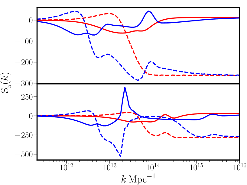
We find that the amplitude of $S_{h}(k)$ for a given model or scenario is maximum around the wave number where the scalar power spectrum exhibits a peak. This is true for both the cases of $S_{h}^{+++}(k)$ and $S_{h}^{+\times\times}(k)$ though there is a certain asymmetry in the behavior of the functions about the peak. Note that the amplitude of $S_{h}(k)$ remains large over large wave numbers, while it quickly reduces to small values at smaller wave numbers. In fact, this behavior should not come as a surprise since such a behavior was also encountered in the case of $\Omega_{{}_{\mathrm{GW}}}(f)$ (cf. figure 8). It is interesting to note that $S_{h}^{+++}(k)$ and $S_{h}^{+\times\times}(k)$ settle down to about $10$ and $-250$, respectively, at large wave numbers. Recall that the secondary tensor bispectra and hence the shape functions we have illustrated in figure 9 have been evaluated during the radiation dominated epoch, when the modes are well inside the Hubble radius. They will have to be evolved until today to examine the corresponding observational imprints which may possibly be detected by upcoming missions such as, say, LISA and PTA (in this context, see ref. [113]; also see refs. [120, 121, 122]).

VII Contributions to PBH formation and secondary GWs from scalar non-Gaussianities

Until now, we have focused on the imprints of the scalar power spectrum on the extent of PBHs formed and the generation of secondary GWs. Clearly, if the scalar non-Gaussianities prove to be large in a given inflationary model, it seems plausible that they would significantly alter the observables $f_{{}_{\mathrm{PBH}}}$, $\Omega_{{}_{\mathrm{GW}}}$ and $S_{h}$ [22, 61, 62, 63, 64, 65, 66, 67, 68, 69, 70, 71, 72]. To understand the possible effects of non-Gaussianities on $f_{{}_{\mathrm{PBH}}}$, $\Omega_{{}_{\mathrm{GW}}}$ as well as $S_{h}$, in this section, we shall first calculate the scalar bispectrum and thereby the corresponding non-Gaussianity parameter $f_{{}_{\rm NL}}$ in the two inflationary models USR2 and PI3 and the reconstructed scenarios RS1 and RS2. We shall then discuss the corresponding contributions from the scalar bispectrum to $f_{{}_{\mathrm{PBH}}}$, $\Omega_{{}_{\mathrm{GW}}}$ and $S_{h}$.

VII.1 Evaluating the scalar bispectrum

The scalar bispectrum is the three point function of the curvature perturbation in Fourier space, and it is defined in terms of the operator $\hat{{\mathcal{R}}}_{\bm{k}}$ that we had introduced earlier as follows [123, 124]:

$$\langle\hat{{\mathcal{R}}}_{{\bm{k}}_{1}}(\eta_{\rm e})\,\hat{{\mathcal{R}}}_{{\bm{k}}_{2}}(\eta_{\rm e})\,\hat{{\mathcal{R}}}_{{\bm{k}}_{3}}(\eta_{\rm e})\rangle=(2\,\pi)^{3}\,{\mathcal{B}}_{{}_{\rm S}}({\bm{k}}_{1},{\bm{k}}_{2},{\bm{k}}_{3})\,\delta^{(3)}({\bm{k}}_{1}+{\bm{k}}_{2}+{\bm{k}}_{3}).$$ (50)

Recall that, $\eta_{\rm e}$ is a time close to the end of inflation and, in this expression, the expectation value on the left hand side is to evaluated in the perturbative vacuum [125, 126, 127]. Note that the three wave vectors $({\bm{k}}_{1},{\bm{k}}_{2},{\bm{k}}_{3})$ form the edges of a triangle. For convenience, we shall hereafter set

$${\mathcal{B}}_{{}_{\rm S}}({\bm{k}}_{1},{\bm{k}}_{2},{\bm{k}}_{3})=(2\,\pi)^{-9/2}\,G({\bm{k}}_{1},{\bm{k}}_{2},{\bm{k}}_{3})$$ (51)

and refer to $G({\bm{k}}_{1},{\bm{k}}_{2},{\bm{k}}_{3})$ as the scalar bispectrum.

The so-called Maldacena formalism is the most complete approach to evaluate the scalar bispectrum in a given inflationary model [125, 126, 127]. In this approach, one first obtains the third order action governing the curvature perturbation. With the third order action at hand, the scalar bispectrum is evaluated using the standard rules of perturbative quantum field theory. For the case of inflation driven by a single, canonical scalar field, the third order action is found to consist of six bulk terms terms, apart from the boundary terms [128]. One can show that the scalar bispectrum $G({\bm{k}}_{1},{\bm{k}}_{2},{\bm{k}}_{3})$ generated by such an action can be expressed as follows (see, for instance, refs. [59, 60]; in this context, also see ref. [36]):

$$G({\bm{k}}_{1},{\bm{k}}_{2},{\bm{k}}_{3}) = \sum_{C=1}^{7}\;G_{{}_{C}}({\bm{k}}_{1},{\bm{k}}_{2},{\bm{k}}_{3})$$ (52)

$$= M_{{}_{\mathrm{Pl}}}^{2}\;\sum_{C=1}^{6}\;\Biggl{[}f_{k_{1}}(\eta_{\rm e})\,f_{k_{2}}(\eta_{\rm e})\,f_{k_{3}}(\eta_{\rm e})\,{\mathcal{G}}_{{}_{C}}({\bm{k}}_{1},{\bm{k}}_{2},{\bm{k}}_{3})+{\mathrm{complex\;conjugate}}\Biggr{]}+G_{7}({\bm{k}}_{1},{\bm{k}}_{2},{\bm{k}}_{3}),$$

where, as we discussed earlier, $f_{k}$ are the positive frequency Fourier modes of the curvature perturbation. Amongst the seven terms in the above expression for the scalar bispectrum, the first six correspond to the bulk terms in the third order action, whereas the seventh arises due to a boundary term, and it is usually absorbed through a field redefinition [128]. The quantities ${\mathcal{G}}_{{}_{C}}({\bm{k}}_{1},{\bm{k}}_{2},{\bm{k}}_{3})$, with $C=(1,6)$, are integrals associated with the bulk terms in the action and, as one can expect, apart from the background quantities, they involve the modes $f_{k}$ and its derivative $f_{k}^{\prime}$. (We have listed these integrals explicitly in appendix C.) The seventh term $G_{7}({\bm{k}}_{1},{\bm{k}}_{2},{\bm{k}}_{3})$ that arises due to the contribution from a boundary term can be expressed as [128, 36]

$$G_{7}({\bm{k}}_{1},{\bm{k}}_{2},{\bm{k}}_{3}) = -i\,M_{{}_{\mathrm{Pl}}}^{2}\,\left[f_{k_{1}}(\eta_{\rm e})\,f_{k_{2}}(\eta_{\rm e})\,f_{k_{3}}(\eta_{\rm e})\right]$$ (53)

$$\times\,\biggl{[}a^{2}\epsilon_{1}\epsilon_{2}\,f_{k_{1}}^{\ast}(\eta)\,f_{k_{2}}^{\ast}(\eta)\,f_{k_{3}}^{\prime\ast}(\eta)+\mathrm{two\leavevmode\nobreak\ permutations}\biggr{]}_{\eta_{i}}^{\eta_{\rm e}}+\leavevmode\nobreak\ \mathrm{complex\leavevmode\nobreak\ conjugate},$$

where $\eta_{\rm i}$ is the time when the initial conditions are imposed on the scalar perturbations. We should mention that the remaining boundary terms do not contribute in the scenarios of our interest.

As in the case of the scalar power spectrum, due to the deviation from slow roll, it proves to be difficult to evaluate the scalar bispectrum analytically in the inflationary models of interest. Therefore, we resort to numerics. There now exists a standard procedure to numerically compute the scalar bispectrum in inflationary models involving a single, canonical scalar field [58, 60]. Recall that, in the case of the power spectrum, it is adequate to impose the Bunch-Davies initial conditions on the modes when they are sufficiently inside the Hubble radius. Apart some special situations wherein the boundary conditions may need to be imposed deeper inside the Hubble, one often imposes the conditions when $k/(a\,H)\simeq 10^{2}$. Since the amplitude of the scalar as well as tensor perturbations freeze when they are adequately outside the Hubble radius, say, when $k/(a\,H)\simeq 10^{-5}$, one can evaluate the power spectra at such a time for the different modes. Note that, in order to arrive at the bispectrum we need to carry out integrals which involve the background quantities, the scalar modes $f_{k}$ and its time derivative $f_{k}^{\prime}$ [cf eqs. (52) and (61)]. These integrals need to be carried out from a time $\eta_{\rm i}$ when the initial conditions are imposed on the modes until the late time $\eta_{\rm e}$ towards the end of inflation. We had mentioned that the amplitudes of the modes freeze soon after they leave the Hubble radius. Due to this reason, one finds that, the super-Hubble contributions to the scalar bispectrum prove to be negligible [60]. Therefore, one can carry out the integrals from the time when $k/(a\,H)\simeq 10^{2}$ to the time when $k/(a\,H)\simeq 10^{-5}$. However, since the bispectrum involves three modes, in general, one needs to integrate from the time when the smallest of the three wave numbers is well inside the Hubble radius to the time until when the largest of the wave numbers is sufficiently outside. Moreover, in order to choose the correct perturbative vacuum, one has to impose a cut-off in the sub-Hubble regime [126]. We impose a democratic (in wave number) cut-off of the form $\mathrm{exp}-\left[\kappa\,(k_{1}+k_{2}+k_{3})/(3\,a\,H)\right]$, where $\kappa$ is a positive definite and small quantity [58, 60, 36]. In fact, such a cut-off aids in the efficient numerical computation of the integrals involved. One can choose a suitable value of $\kappa$ depending on how deep from inside the Hubble radius the integrals are to be carried out.

VII.2 Amplitude and shape of $f_{{}_{\rm NL}}$

The non-Gaussianity parameter, say, $f_{{}_{\rm NL}}({\bm{k}}_{1},{\bm{k}}_{2},{\bm{k}}_{3})$, corresponding to the scalar bispectrum is defined as (see, for instance, Refs. [59, 60])

$$f_{{}_{\rm NL}}({\bm{k}}_{1},{\bm{k}}_{2},{\bm{k}}_{3}) = -\frac{10}{3}\,\frac{1}{\left(2\,\pi\right)^{4}}\;k_{1}^{3}\,k_{2}^{3}\,k_{3}^{3}\;G({\bm{k}}_{1},{\bm{k}}_{2},{\bm{k}}_{3})\,\biggl{[}k_{1}^{3}\,\mathcal{P}_{{}_{\mathrm{S}}}(k_{2})\,\mathcal{P}_{{}_{\mathrm{S}}}(k_{3})+{\mathrm{two\leavevmode\nobreak\ permutations}}\biggr{]}^{-1},$$ (54)

where $\mathcal{P}_{{}_{\mathrm{S}}}(k)$ denotes the scalar power spectrum [cf. eq. (11a)]. With the scalar power and bispectra at hand, evidently, it is straightforward to arrive the non-Gaussianity parameter $f_{{}_{\rm NL}}$ for a given model.

Based on prior experience, we would like to emphasize a few points concerning the expected shape and amplitude of the scalar bispectrum before we go on to present the results for $f_{{}_{\rm NL}}$ in the different models and scenarios we have introduced earlier. As is well known, in slow roll inflationary models involving a single, canonical scalar field, the scalar non-Gaussianity parameter $f_{{}_{\rm NL}}$ proves to be of the order of the first slow roll parameter $\epsilon_{1}$ [125, 126, 127]. In other words, the parameter $f_{{}_{\rm NL}}$ is typically of the order of $10^{-2}$ or smaller in such situations. Moreover, the bispectrum is found to have an equilateral shape, with the $f_{{}_{\rm NL}}$ parameter slightly peaking when $k_{1}=k_{2}=k_{3}$ (in this context, see, for instance, ref. [60]). However, when departures from slow roll occur, the non-Gaussianity parameter $f_{{}_{\rm NL}}$ can be expected to be of the order of unity or larger, depending on the details of the background dynamics. Further, in contrast to the slow roll case, wherein there is only a weak dependence of the parameter $f_{{}_{\rm NL}}$ on scale, when departures from slow roll occur, the parameter turns out to be strongly scale dependent. Needless to say, we can expect that the non-Gaussianity parameter $f_{{}_{\rm NL}}$ to be relatively large as well as strongly scale dependent in the situations of our interest.

Let us now discuss the results we obtain in the different models we have introduced. In order to illustrate the complete shape of the bispectrum, the non-Gaussianity parameter $f_{{}_{\rm NL}}$ is usually presented as a density plot in, say, the $(k_{3}/k_{1})$-$(k_{2}/k_{1})$-plane [60, 129]. It proves to be a bit of a numerical challenge to compute the complete shape of the bispectrum across the wide range of wave numbers over which we have evaluated the power spectra. As a result, we shall focus on the amplitude of $f_{{}_{\rm NL}}$ in the equilateral and the squeezed limits, i.e. when $k_{1}=k_{2}=k_{3}=k$ and when $k_{1}\to 0$, $k_{2}\simeq k_{3}=k$, respectively. It is easier to calculate the scalar bispectrum in the equilateral limit as we just need to follow the evolution of one mode at a time. To arrive at the scalar bispectrum in the squeezed limit, we shall set $k_{2}=k_{3}=k$ and choose $k_{1}=10^{-3}\,k$. We have confirmed that our results are robust against choosing a smaller value of $k_{1}$. Before we go to illustrate the amplitude and shape of the non-Gaussianity parameter $f_{{}_{\rm NL}}$, let us understand the behavior of the scalar bispectrum $G({\bm{k}}_{1},{\bm{k}}_{2},{\bm{k}}_{3})$ itself. In figure 10, we have plotted the scalar bispectra that arise in the equilateral and squeezed limits in the models of USR2 and PI3.

Figure 10: The amplitude of the dimensionless scalar bispectra has been plotted in the equilateral (on top) and squeezed limits (at the bottom) for the models USR2 (in red) and PI3 (in blue). Clearly, the bispectra have approximately the same shape as the corresponding power spectra (cf. figure 4). Note that, at small scales, the dimensionless bispectra have considerably lower amplitudes in the squeezed limit when compared to their values in the equilateral limit, whereas they have roughly the same amplitude over the CMB scales.

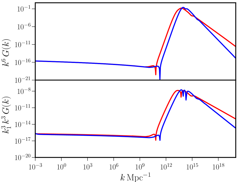
We would like to highlight a few aspects regarding the amplitude and shape of the bispectra. Note that the scalar bispectra have roughly the same shape in the equilateral and squeezed limits. Also, they closely resemble the corresponding scalar power spectra and, in particular, they exhibit a dip and a peak around the same locations (cf. figure 4). Moreover, at small scales, the scalar bispectra have a larger amplitude in the equilateral limit than in the squeezed limit. Further, in the equilateral limit, the scalar bispectra have almost the same amplitude as the power spectra near the peak.

Let us now understand the behavior of the non-Gaussianity parameter $f_{{}_{\rm NL}}$. In figures 11 and 12, we have plotted the behavior of the $f_{{}_{\rm NL}}$ parameter in the equilateral and squeezed limits over a wide range of wave numbers in the models USR2 and PI3 as well as the scenarios RS1 and RS2.

Figure 11: The scalar non-Gaussianity parameter $f_{{}_{\rm NL}}$ has been plotted in the equilateral (on top) and the squeezed (at the bottom) limits for the model of USR2 (in red) and the reconstructed scenario RS1 (in blue and green). Note that, in the case of RS1, we have worked with our original choice of $N_{1}=42$ and plotted the lower (in blue) and the upper (in green) bounds of $f_{{}_{\rm NL}}$ corresponding to the range over which the parameter $\Delta N_{1}$ is varied. In the case of USR2, we have also plotted the consistency condition $f_{{}_{\rm NL}}^{{}_{\mathrm{CR}}}(k)=(5/12)\,[n_{{}_{\mathrm{S}}}(k)-1]$ (as purple dots) along with the results in the squeezed limit. Despite the deviations from slow roll leading to strong features in the scalar power and bispectra, we find that the consistency condition is always satisfied. The insets highlight the $f_{{}_{\rm NL}}$ around the wave numbers where the scalar power spectra exhibit their peaks. It is clear that the parameter $f_{{}_{\rm NL}}$ attains larger values in the equilateral (where $f_{{}_{\rm NL}}\simeq 10^{1}$–$10^{4}$ at its maximum) than the squeezed (where $f_{{}_{\rm NL}}\simeq 1$–$10$) limit. Importantly, we find that $f_{{}_{\rm NL}}$ is at most of order unity near the peaks of the scalar power spectra.

Figure 12: The scalar non-Gaussianity parameter $f_{{}_{\rm NL}}$ has been plotted in the equilateral and the squeezed limits for the model PI3 and the reconstructed scenario RS2 in the same manner (and the same choices of colors) as in the cases of USR2 and RS1 in the previous figure. In the case of RS2, we have worked with our initial choice of $N_{1}=48$ and plotted the lower (in blue) and the upper (in green) bounds of $f_{{}_{\rm NL}}$ corresponding to the range over which the parameter $\Delta N_{1}$ is varied. It should be evident that our earlier comments regarding the results for USR2 and RS1 apply to the cases of PI3 and RS2 as well.

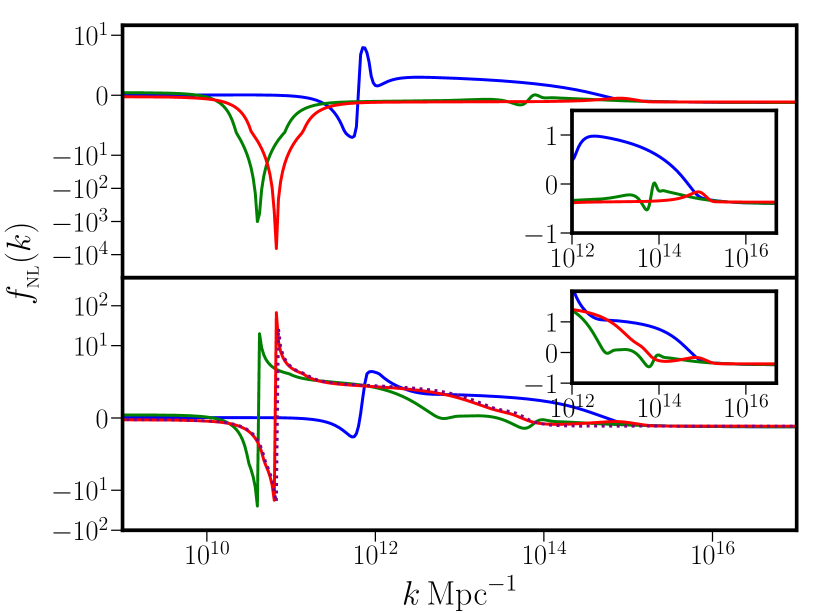
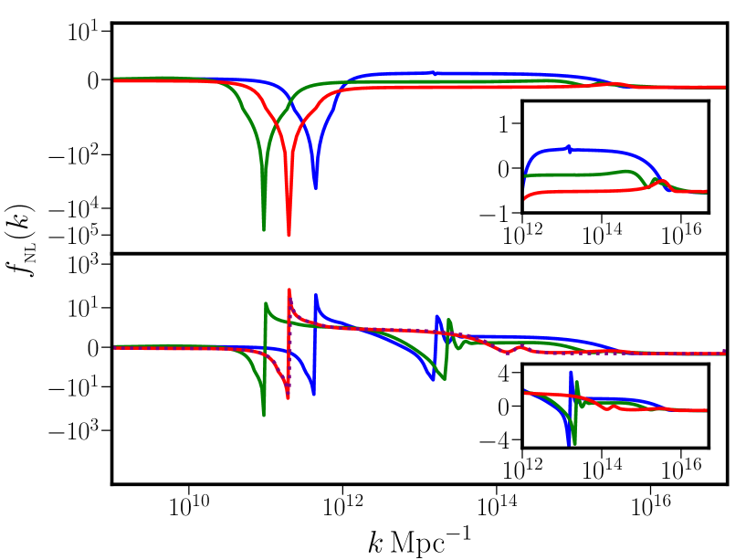
The following points are evident from the two figures. Firstly, in the equilateral limit, the non-Gaussianity parameter $f_{{}_{\rm NL}}$ proves to be fairly large (of the order of $10^{1}$–$10^{4}$) over a small range of wave numbers. In fact, the $f_{{}_{\rm NL}}$ exhibit an upward spike in their amplitude around exactly the same wave numbers wherein the scalar power spectra exhibit a downward spike (cf. figures 4 and 6). Since the definition of the parameter $f_{{}_{\rm NL}}$ [cf. eq. (54)] contains the scalar power spectrum in the denominator, the upward spike can be partly attributed to the downward spike in the power spectrum. If we ignore the large spike, we find that $f_{{}_{\rm NL}}\simeq 1$–$10$ around these wave numbers. It is worth noting that these wave numbers correspond to those modes which leave the Hubble radius just prior to or during the transition from the slow roll to the ultra slow roll regime. In contrast, the non-Gaussianity parameter $f_{{}_{\rm NL}}$ proves to be relatively small (at most of order unity) over wave numbers where the scalar power spectra exhibit their peak. However, we should clarify that, though the value of $f_{{}_{\rm NL}}$ is smaller than unity around this domain, it is considerably larger than its typical value in slow roll inflation (of about $10^{-2}$, such as over the CMB scales in our models). For instance, in USR2 and PI3, we find that, in the equilateral limit, $f_{{}_{\rm NL}}$ is about $-0.37$ and $-0.44$, respectively, near the locations of the peak in the power spectra. This can be attributed to the large value of $\epsilon_{2}$ during the ultra slow roll regime. Secondly, in the squeezed limit, the scalar bispectrum is expected to satisfy the so called consistency condition wherein it can be completely expressed in terms of the scalar power spectrum [125, 130]. This translates to the condition $f_{{}_{\rm NL}}^{{}_{\mathrm{CR}}}(k)=(5/12)\,[n_{{}_{\mathrm{S}}}(k)-1]$ in the squeezed limit, where $n_{{}_{\mathrm{S}}}(k)-1={\mathrm{d}}\,\mathrm{ln}\,\mathcal{P}_{{}_{\mathrm{S}}}(k)/{\mathrm{d}}\,\mathrm{ln}\,k$ is the scalar spectral index. In figures 11 and 12, apart from plotting $f_{{}_{\rm NL}}$ in the squeezed limit, we have also plotted the quantity $f_{{}_{\rm NL}}^{{}_{\mathrm{CR}}}$ obtained from the scalar spectral index. We should add that we have also examined the validity of the consistency relation more closely by working with a smaller $k_{1}$. We find that the consistency condition is indeed satisfied even when there arise strong features in the scalar power spectrum in all the scenarios of our interest (in this context, however, see appendix D). Therefore, in the squeezed limit, we find that $f_{{}_{\rm NL}}$ is at most of order unity around the peaks of the scalar power spectra.

It seems important that we clarify a point regarding the validity of the consistency condition at this stage of our discussion. One may be concerned if the period of ultra slow roll, with its large value of $\epsilon_{2}$, could lead to a violation of the consistency condition over wave numbers that leave the Hubble radius during this epoch (in this context, see refs. [131, 132, 133]). Recall that the amplitude of scalar modes over a certain range of wave numbers are modified to some extent during the transition from slow roll to ultra slow roll (cf. figure 3). However, since, in the cases of our interest, the epoch of ultra slow roll ends leading to the eventual termination of inflation, the amplitude of the scalar modes asymptotically freeze at sufficiently late times (for further details, see appendix E; in this context, also see refs. [134, 69]). Due to this asymptotic behavior of the scalar modes, it should not come as a surprise that the consistency condition is satisfied in the models and scenarios of our interest despite the phase of ultra slow roll (for very recent discussions in this context, see Refs. [135, 136]).

VII.3 Imprints of $f_{{}_{\rm NL}}$ on $f_{{}_{\mathrm{PBH}}}$ and $\Omega_{{}_{\mathrm{GW}}}$

Recall that the observationally relevant dimensionless, scalar non-Gaussianity parameter $f_{{}_{\rm NL}}$ is usually introduced through the following relation (see ref. [137]; also see refs. [59, 60]):

$${\mathcal{R}}(\eta,{\bm{x}})={\mathcal{R}}^{\mathrm{G}}(\eta,{\bm{x}})-\frac{3}{5}\,f_{{}_{\rm NL}}\,\left[{\mathcal{R}}^{{}_{\mathrm{G}}}(\eta,{\bm{x}})\right]^{2}$$ (55)

where ${\mathcal{R}}^{\mathrm{G}}$ denotes the Gaussian contribution. In Fourier space, this relation can be written as (see, for instance, ref. [59])

$${\mathcal{R}}_{\bm{k}}={\mathcal{R}}^{\mathrm{G}}_{\bm{k}}-\frac{3}{5}\,f_{{}_{\rm NL}}\,\int\frac{{\mathrm{d}}^{3}{{\bm{p}}}}{(2\,\pi)^{3/2}}\,{\mathcal{R}}^{\mathrm{G}}_{{\bm{p}}}\;{\mathcal{R}}^{\mathrm{G}}_{{\bm{k}}-{\bm{p}}}.$$ (56)

If one uses this expression for ${\mathcal{R}}_{\bm{k}}$ and evaluates the corresponding two-point correlation function in Fourier space, one obtains that [71, 72]

$$\langle\hat{{\mathcal{R}}}_{\bm{k}}\,\hat{{\mathcal{R}}}_{{\bm{k}}^{\prime}}\rangle=\frac{2\,\pi^{2}}{k^{3}}\,\delta^{(3)}({\bm{k}}+{\bm{k}}^{\prime})\,\left[\mathcal{P}_{{}_{\mathrm{S}}}(k)+\left(\frac{3}{5}\right)^{2}\,\frac{k^{3}}{2\,\pi}\,f_{{}_{\rm NL}}^{2}\,\int{\rm d}^{3}{{\bm{p}}}\,\frac{\mathcal{P}_{{}_{\mathrm{S}}}(p)}{p^{3}}\,\frac{\mathcal{P}_{{}_{\mathrm{S}}}\left(|{\bm{k}}-{\bm{p}}|\right)}{|{\bm{k}}-{\bm{p}}|^{3}}\right],$$ (57)

where $\mathcal{P}_{{}_{\mathrm{S}}}(k)$ is the original scalar power spectrum defined in the Gaussian limit [cf. eq. (10a)], while the second term represents the leading non-Gaussian correction. We find that we can write the non-Gaussian correction to the scalar power spectrum, say, $\mathcal{P}_{{}_{\mathrm{C}}}(k)$, as follows:

$$\mathcal{P}_{{}_{\mathrm{C}}}(k) = \left(\frac{3}{5}\right)^{2}\,f_{{}_{\rm NL}}^{2}\,\int_{0}^{\infty}{\mathrm{d}}v\int_{|1-v|}^{1+v}\frac{{\mathrm{d}}u}{v^{2}\,u^{2}}\,\mathcal{P}_{{}_{\mathrm{S}}}(k\,v)\,\mathcal{P}_{{}_{\mathrm{S}}}(k\,u)$$ (58)

$$= \left(\frac{12}{5}\right)^{2}\,f_{{}_{\rm NL}}^{2}\,\int_{0}^{\infty}{\mathrm{d}}s\int_{0}^{1}\frac{{\mathrm{d}}d}{(s^{2}-d^{2})^{2}}\,\mathcal{P}_{{}_{\mathrm{S}}}[k\,(s+d)/2]\,\mathcal{P}_{{}_{\mathrm{S}}}[k\,(s-d)/2].$$

Since we have evaluated the scalar non-Gaussianity parameter in the inflationary models of our interest, we can now calculate the non-Gaussian corrections $\mathcal{P}_{{}_{\mathrm{C}}}(k)$ to the scalar power spectrum and the corresponding modifications to $f_{{}_{\mathrm{PBH}}}$, $\Omega_{{}_{\mathrm{GW}}}$ and $S_{h}$. However, before we do so, we need to clarify an important point. In introducing the scalar non-Gaussianity parameter through the relation (55), it has been assumed that $f_{{}_{\rm NL}}$ is local, i.e. it is independent of the wave number [137]. In contrast, the parameter $f_{{}_{\rm NL}}$ proves to be strongly scale dependent in all the situations we have considered. In order to be consistent with the fact that the $f_{{}_{\rm NL}}$ in eq. (55) is local, we shall consider the squeezed limit of the parameter (in this context, also see the discussions in ref. [63]). Moreover, in the expression (58) for $\mathcal{P}_{{}_{\mathrm{C}}}(k)$, we shall assume that $f_{{}_{\rm NL}}$ is dependent on the wave number $k$, with $k_{2}=k_{3}\simeq k$ and $k_{1}\ll k$ to be consistent with the squeezed limit. In figure 13, we have plotted the original Gaussian power spectrum as well the modified power spectrum including the non-Gaussian corrections $\mathcal{P}_{{}_{\mathrm{C}}}(k)$.

Figure 13: The original scalar power spectrum $\mathcal{P}_{{}_{\mathrm{S}}}(k)$ (in solid red) and the modified spectrum $\mathcal{P}_{{}_{\mathrm{S}}}(k)+\mathcal{P}_{{}_{\mathrm{C}}}(k)$ (in dashed blue) arrived at upon including the non-Gaussian corrections, have been plotted for the models of USR2 (on top) and PI3 (at the bottom). In these models, the non-Gaussianity parameter $f_{{}_{\rm NL}}$ had exhibited sharp spikes in its amplitude around wave numbers where the Gaussian scalar power spectrum had contained downward spikes. We should clarify here that, in order to arrive at the modified power spectra, we have regulated the spikes in the $f_{{}_{\rm NL}}$ parameter so that its maximum value around these wave numbers is $10^{2}$. Clearly, the modifications to the scalar spectra, particularly at their peak, is hardly significant.

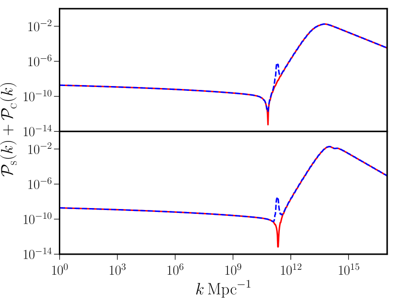
Recall that the non-Gaussianity parameter $f_{{}_{\rm NL}}$ had contained sharp spikes around the wave numbers where the Gaussian scalar power spectra had exhibited a downward spike (cf. figures 11 and 12). While evaluating the modified power spectra, we have regulated the maximum value of these spikes to be $|f_{{}_{\rm NL}}|\simeq 100$. Evidently, the non-Gaussian corrections to the scalar power spectrum are insignificant. This can be attributed to the fact that the peaks in the original power spectrum $\mathcal{P}_{{}_{\mathrm{S}}}(k)$ and the non-Gaussianity parameter $f_{{}_{\rm NL}}$ are located at different wave numbers. Therefore, we find the corresponding modifications to $f_{{}_{\mathrm{PBH}}}$, $\Omega_{{}_{\mathrm{GW}}}$ and $S_{h}$ are insignificant as well. This conclusion can also be understood from the fact the amplitude of the dimensionless bispectrum in the squeezed limit is considerably smaller than the amplitude of the scalar power spectrum around its peak (cf. figure 10).

We should clarify a particular point regarding the non-Gaussian corrections we have calculated in this section. Note that we have calculated the cubic order non-Gaussian corrections to the power spectrum. This method proves to be adequate to examine the imprints of non-Gaussianities on the dimensionless energy density $\Omega_{{}_{\mathrm{GW}}}$ describing the secondary GWs. However, the approach does not completely account for the effects of non-Gaussianities on the fraction $f_{{}_{\mathrm{PBH}}}$ of PBHs produced (for an early discussion on the topic, see ref. [138]; for recent discussions, see refs. [139, 140]). In the context of PBHs, the non-Gaussianities also change the shape of the probability distribution characterizing the over-densities at the time of their formation, which we have assumed to be a Gaussian [cf. eq. (17)] These effects due to the non-Gaussianities are expected to be larger (than the corrections to the power spectrum we have calculated), and they need to be taken into account to arrive at the modified $f_{{}_{\mathrm{PBH}}}$ [139].

VIII Conclusions

In this work, we had considered models involving a single, canonical scalar field that lead to ultra slow roll or punctuated inflation. All these models had contained a point of inflection, which seems essential to achieve the epoch of ultra slow roll required to enhance scalar power on small scales. We had also examined the extent of PBHs formed and the secondary GWs generated in these models and had compared them with the constraints on the corresponding observables $f_{{}_{\mathrm{PBH}}}$ and $\Omega_{{}_{\mathrm{GW}}}$. These models require a considerable extent of fine tuning in order to lead to the desirable duration of inflation (of say, $60$–$70$ e-folds), be consistent with the constraints from the CMB on large scales, and simultaneously exhibit higher scalar power on small scales.

In order to explore the possibilities in single field models further, we had also considered scenarios wherein the functional forms for the first slow roll parameter closely mimic the typical behavior in ultra slow roll and punctuated inflation. We had reconstructed the potentials associated with these scenarios, evaluated the resulting scalar and tensor power spectra as well as the corresponding imprints on $f_{{}_{\mathrm{PBH}}}$, $\Omega_{{}_{\mathrm{GW}}}$ and $S_{h}$. The presence of extra parameters in the choices for $\epsilon_{1}(N)$ had allowed us to construct the required scenarios rather easily. Interestingly, we had found that the reconstructed potentials too contain a point of inflection as the original models do. This lends further credence to the notion that a point of inflection is essential to achieve ultra slow roll or punctuated inflation. However, we should add a note of caution that, while we were able to broadly capture the expected shape of the scalar power spectra in the reconstructed scenarios, there were some differences in the tensor power spectra in these scenarios and the original models. Moreover, we find that these reconstructed scenarios allow us to easily examine the rate of growth of the scalar power from the CMB scales to small scales (for a discussion in this context, see refs. [76, 81]). While the steepest growth possible in the reconstructed scenario RS1 has $n_{{}_{\mathrm{S}}}-1\simeq 4$, we find that the growth is non-uniform but faster in RS2 with $n_{{}_{\mathrm{S}}}-1$ between $4$ and $6$ over the relevant range of wave numbers (for details, see appendix F). Further, though we have been able to reconstruct the potentials numerically in the scenarios RS1 and RS2, it would be worthwhile to arrive at analytical forms of these potentials [75, 76, 77].

We had also computed the scalar bispectrum and the associated non-Gaussianity parameter $f_{{}_{\rm NL}}$ is these models and scenarios. We had found that the parameter $f_{{}_{\rm NL}}$ is strongly scale dependent in all the cases. Also, the non-Gaussianities had turned out to be fairly large (with, say, $f_{{}_{\rm NL}}>10$ over a range of wave numbers) in the equilateral limit. Moreover, we had found that the consistency condition governing the non-Gaussianity parameter is always satisfied, despite the period of sharp departure from slow roll, implying that the non-Gaussianity parameter in the squeezed limit is at most of order unity around the domain where the scalar power spectra exhibit their peak. Due to this reason, we had found that the non-Gaussian corrections to power spectra were negligible leading to insignificant modifications to the observables $f_{{}_{\mathrm{PBH}}}$, $\Omega_{{}_{\mathrm{GW}}}$ and $S_{h}$ on small scales. However, we should point out that the effects of non-Gaussianities on $f_{{}_{\mathrm{PBH}}}$ and $\Omega_{{}_{\mathrm{GW}}}$ have been included in a simple fashion and a more detailed approach seems required to account for the complicated scale dependence of $f_{{}_{\rm NL}}$ [64, 65, 66, 64, 68, 69]. It has recently been argued that, in the squeezed limit of the bispectrum, the part satisfying the consistency relation should be subtracted away as it cannot be observed (in this context, see refs. [141, 142]; however also see Ref. [143]). If this is indeed so, since the scalar bispectrum satisfies the consistency condition in the squeezed limit in the models and scenarios we have examined, the cubic order non-Gaussian corrections to the power spectrum would then identically vanish.

Moreover, we had calculated the secondary tensor bispectrum generated in the different inflationary models of interest during the radiation dominated epoch. Interestingly, we had found that the shape function characterizing the tensor bispectrum has an amplitude of about $10$–$250$ at small wave numbers in all the models and scenarios of interest. It seems important to evolve the shape function until today and examine the possibility of observing its imprints in ongoing efforts such as PTA [120] and forthcoming missions such as LISA [113, 121, 122]. We are currently investigating these issues in a variety of single and two field models of inflation [144, 145, 146, 147, 148, 149, 150, 151, 152].

Appendix A The dichotomy of ultra slow roll and punctuated inflation

With the help of an example, in this appendix, we shall illustrate that a given inflationary potential can permit ultra slow roll as well as punctuated inflation for different sets of parameters. The potential that we shall consider, when expressed in terms of the quantity $x=\phi/v$ that we had introduced in the context of USR1, is given by [29]

$$V(\phi)=V_{0}\,\frac{\alpha\,x^{2}-\beta\,x^{4}+\gamma\,x^{6}}{(1+\delta\,x^{2})^{2}}.$$ (59)

In figure 14, we have plotted the evolution of the first slow roll parameter $\epsilon_{1}$ in the above potential for the following two sets of parameters: $V_{0}/M_{{}_{\mathrm{Pl}}}^{4}=1.3253\times 10^{-9}$, $\gamma=1$, $\delta=1.5092$ and $(v/M_{{}_{\mathrm{Pl}}},\alpha,\beta)=(4.3411,8.522\times 10^{-2},0.469)$ and $(10,8.53\times 10^{-2},0.458)$.

Figure 14: The behavior of the first slow roll parameter $\epsilon_{1}$ has been plotted for two sets of parameters describing the potential (59) and suitable initial conditions that lead to about $75$ e-folds of inflation. Note that the first set of values for the parameters leads to punctuated inflation with $\epsilon_{1}$ (plotted in red) crossing unity (indicated as a dotted horizontal line) twice, once prior to the regime of ultra slow roll and eventually when inflation terminates. The second set of parameters leads to an extended period of ultra slow roll (plotted in blue) without any interruption of inflation until the very end.

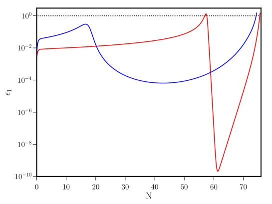
We obtain about $75$ e-folds of inflation in these cases for $\phi_{\mathrm{i}}=17.245\,M_{{}_{\mathrm{Pl}}}$ and $\phi_{\mathrm{i}}=13.4\,M_{{}_{\mathrm{Pl}}}$. It is clear from the figure that, while the first set of parameters lead to punctuated inflation, the second set does not permit an interruption of inflation until the very end. This example illustrates the point that a potential itself cannot be classified as an ultra slow roll or a punctuated inflationary model.

Appendix B The functional forms of the polarization factors

Recall that, $e^{\lambda}({\bm{k}},{\bm{p}})=e_{ij}^{\lambda}({\bm{k}})\,p^{i}\,p^{j}$. For our choice of $({\bm{k}}_{1},{\bm{k}}_{2},{\bm{k}}_{3})$ and $({\bm{p}}_{1},{\bm{p}}_{2},{\bm{p}}_{3})$ [cf. eqs. (46) and (47)], we find that $e^{\lambda}({\bm{k}},{\bm{p}})$ can be evaluated to be

$$e^{+}({\bm{k}}_{1},{\bm{p}}_{1}) = \frac{1}{4\,\sqrt{2}}\,\left(3\,p_{1x}^{2}+p_{1y}^{2}-2\,\sqrt{3}\,p_{1x}\,p_{1y}-4\,p_{1z}^{2}\right),$$ (60a)

$$e^{+}({\bm{k}}_{2},{\bm{p}}_{2}) = \frac{1}{4\,\sqrt{2}}\,\biggl{(}3\,p_{1x}^{2}+3\,k^{2}+p_{1y}^{2}+2\,\sqrt{3}\,p_{1x}\,p_{1y}-6\,k\,p_{1x}-2\,\sqrt{3}\,k\,p_{1y}-4\,p_{1z}^{2}\biggr{)},$$ (60b)

$$e^{+}({\bm{k}}_{3},{\bm{p}}_{3}) = \frac{1}{\sqrt{2}}\,\left(p_{1y}^{2}-p_{1z}^{2}\right),$$ (60c)

$$e^{\times}({\bm{k}}_{1},{\bm{p}}_{1}) = -\frac{1}{\sqrt{2}}\,\left(\sqrt{3}\,p_{1x}-p_{1y}\right)\,p_{1z},$$ (60d)

$$e^{\times}({\bm{k}}_{2},{\bm{p}}_{2}) = \frac{1}{\sqrt{2}}\,\left[\sqrt{3}\,(p_{1x}-k)+p_{1y}\right]\,p_{1z},$$ (60e)

$$e^{\times}({\bm{k}}_{3},{\bm{p}}_{3}) = -\sqrt{2}\,p_{1y}\,p_{1z}.$$ (60f)

Appendix C Integrals determining the scalar bispectrum

The quantities ${\mathcal{G}}_{{}_{C}}({\bm{k}}_{1},{\bm{k}}_{2},{\bm{k}}_{3})$ appearing in the expression (52) for the scalar bispectrum represent six integrals that involve the scale factor, the slow roll parameters, the modes $f_{k}$ and their time derivatives $f_{k}^{\prime}$. They correspond to the six bulk terms appearing in the cubic order action governing the curvature perturbation, and they are described by the following expressions [59, 60, 36]:

$${\mathcal{G}}_{1}({\bm{k}}_{1},{\bm{k}}_{2},{\bm{k}}_{3}) = 2\,i\,\int_{\eta_{\rm i}}^{\eta_{\rm e}}{\mathrm{d}}\eta\;a^{2}\,\epsilon_{1}^{2}\,\left(f_{k_{1}}^{\ast}\,f_{k_{2}}^{\prime\ast}\,f_{k_{3}}^{\prime\ast}+{\mathrm{two\leavevmode\nobreak\ permutations}}\right),$$ (61a)

$${\mathcal{G}}_{2}({\bm{k}}_{1},{\bm{k}}_{2},{\bm{k}}_{3}) = -2\,i\;\left({\bm{k}}_{1}\cdot{\bm{k}}_{2}+{\mathrm{two\leavevmode\nobreak\ permutations}}\right)\,\int_{\eta_{\rm i}}^{\eta_{\rm e}}{\mathrm{d}}\eta\;a^{2}\,\epsilon_{1}^{2}\,f_{k_{1}}^{\ast}\,f_{k_{2}}^{\ast}\,f_{k_{3}}^{\ast},$$ (61b)

$${\mathcal{G}}_{3}({\bm{k}}_{1},{\bm{k}}_{2},{\bm{k}}_{3}) = -2\,i\,\int_{\eta_{\rm i}}^{\eta_{\rm e}}{\mathrm{d}}\eta\;a^{2}\,\epsilon_{1}^{2}\,\left(\frac{{\bm{k}}_{1}\cdot{\bm{k}}_{2}}{k_{2}^{2}}\,f_{k_{1}}^{\ast}\,f_{k_{2}}^{\prime\ast}\,f_{k_{3}}^{\prime\ast}+{\mathrm{five\leavevmode\nobreak\ permutations}}\right),$$ (61c)

$${\mathcal{G}}_{4}({\bm{k}}_{1},{\bm{k}}_{2},{\bm{k}}_{3}) = i\,\int_{\eta_{\rm i}}^{\eta_{\rm e}}{\mathrm{d}}\eta\;a^{2}\,\epsilon_{1}\,\epsilon_{2}^{\prime}\,\left(f_{k_{1}}^{\ast}\,f_{k_{2}}^{\ast}\,f_{k_{3}}^{\prime\ast}+{\mathrm{two\leavevmode\nobreak\ permutations}}\right),$$ (61d)

$${\mathcal{G}}_{5}({\bm{k}}_{1},{\bm{k}}_{2},{\bm{k}}_{3}) = \frac{i}{2}\,\int_{\eta_{\rm i}}^{\eta_{\rm e}}{\mathrm{d}}\eta\;a^{2}\,\epsilon_{1}^{3}\;\left(\frac{{\bm{k}}_{1}\cdot{\bm{k}}_{2}}{k_{2}^{2}}\,f_{k_{1}}^{\ast}\,f_{k_{2}}^{\prime\ast}\,f_{k_{3}}^{\prime\ast}+{\mathrm{five\leavevmode\nobreak\ permutations}}\right),$$ (61e)

$${\mathcal{G}}_{6}({\bm{k}}_{1},{\bm{k}}_{2},{\bm{k}}_{3}) = \frac{i}{2}\,\int_{\eta_{\rm i}}^{\eta_{\rm e}}{\mathrm{d}}\eta\,a^{2}\,\epsilon_{1}^{3}\,\left(\frac{k_{1}^{2}\,\left({\bm{k}}_{2}\cdot{\bm{k}}_{3}\right)}{k_{2}^{2}\,k_{3}^{2}}\,f_{k_{1}}^{\ast}\,f_{k_{2}}^{\prime\ast}\,f_{k_{3}}^{\prime\ast}+{\mathrm{two\leavevmode\nobreak\ permutations}}\right).\qquad$$ (61f)

These integrals are to be evaluated from a sufficiently early time, say, $\eta_{\rm i}$, when all the modes are well inside the Hubble radius, until suitably late times, which can be conveniently chosen to be a time close to the end of inflation, say, $\eta_{\rm e}$.

Appendix D A closer examination of the consistency relation

We had pointed out that, in the squeezed limit, i.e. when $k_{2}\simeq k_{3}=k$ and $k_{1}\to 0$, the non-Gaussianity parameter $f_{{}_{\rm NL}}$ is expected to satisfy the consistency condition $f_{{}_{\rm NL}}^{{}_{\mathrm{CR}}}(k)=(5/12)\,[n_{{}_{\mathrm{S}}}(k)-1]$, where $n_{{}_{\mathrm{S}}}(k)-1={\mathrm{d}}\,\mathrm{ln}\,\mathcal{P}_{{}_{\mathrm{S}}}(k)/{\mathrm{d}}\,\mathrm{ln}\,k$ is the scalar spectral index. In the results presented earlier (in figures 11 and 12), we had worked with $k_{1}=10^{-3}\,k$ to arrive at $f_{{}_{\rm NL}}$ in the squeezed limit. While we find that the consistency condition is satisfied to better than $5\%$ over a wide range of scales, we notice that there is some departure around wave numbers corresponding to the peak in the scalar power spectrum. To investigate this point more closely, in figure 15, we have plotted the numerical results around the peak in the scalar power spectrum for the original choice of $k_{1}$ as well as for $k_{1}=10^{-1}\,k$ and $k_{1}=10^{-5}\,k$ in the case of the model PI3.

Figure 15: The non-Gaussianity parameter $f_{{}_{\rm NL}}$ in the squeezed limit (in blue) and the consistency condition $f_{{}_{\rm NL}}^{{}_{\mathrm{CR}}}$ (in red) have been plotted for the model PI3 over wave numbers around the peak in the scalar power spectrum. We have set the squeezed mode to be $k_{1}=10^{-1}\,k$ (on the left), $k_{1}=10^{-3}\,k$ (in the middle) and $k_{1}=10^{-5}\,k$ (on the right) in plotting these figures. We have also indicated the $5\%$ uncertainty in our numerical estimate as bands (in blue). Moreover, we have demarcated the range of modes (by vertical, dashed, green lines) that leave the Hubble radius during the epoch of ultra slow roll in the model. Obviously, the choice of $k_{1}=10^{-1}\,k$ is insufficient for $k_{1}$ to be considered a squeezed mode. Such a choice has been made to illustrate the point that the value of $f_{{}_{\rm NL}}$ proves to be of order unity even when we confine to modes that leave the Hubble radius during the period of ultra slow roll. Evidently, there is an improvement in the extent to which the consistency condition is satisfied when we choose to work with smaller and smaller values of $k_{1}$. Though the match improves as we work with a smaller $k_{1}$, we still seem to notice some deviation. This is possibly an artefact arising due to the reason that, numerically, we are unable to work with an adequately small value of $k_{1}$.

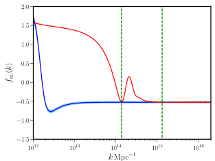
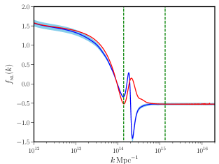
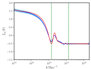
We have considered the case of $k_{1}=10^{-1}\,k$ since we find that roughly a decade of modes exit the Hubble radius during the ultra slow roll phase. Evidently, such a value of $k_{1}$ would be insufficient for it to be considered a squeezed mode. We find that the value of $f_{{}_{\rm NL}}$ remains of order unity even when we confine to modes which leave the Hubble radius during the period of ultra slow roll. Also, as one would expect, we find that the consistency condition is satisfied better and better as we work with a smaller value of $k_{1}$. We should clarify that adequate care needs to be taken while evaluating the integrals involved in the calculation of the bispectrum during the ultra slow roll regime. Since there occur rapid changes in the slow roll parameters during this epoch, we should regulate the integrals with an appropriate choice for the cut-off parameter $\kappa$, especially for the dominant contribution $G_{4}({\bm{k}}_{1},{\bm{k}}_{2},{\bm{k}}_{3})$ [cf. appendix C]. With an appropriate cut-off and with smaller values for the squeezed mode $k_{1}$, we find that the match between $f_{{}_{\rm NL}}$ and $f_{{}_{\rm NL}}^{{}_{\mathrm{CR}}}$ indeed improves. Nevertheless, even with a smaller of choice of $k_{1}$, we still notice some difference near the peak in the power spectrum. We feel that this is an artefact and we believe that the difference can be overcome with a further smaller value for $k_{1}$. However, working with a very small $k_{1}$ poses certain numerical challenges, and we will leave it for future investigation. We should mention that this an independent issue and stress that it does not affect our main conclusions related to PBHs and GWs.

Appendix E Asymptotic behavior of the curvature perturbations

As we mentioned, it has been shown that an indefinite ultra slow roll regime of inflation leads to the violation of the consistency condition [131, 132]. Since all the models of our interest contain an ultra slow roll phase, one may wonder if a violation of the consistency condition would occur in these cases. As we have seen, the consistency condition is satisfied in all the cases we have considered. This is primarily due to the fact that the ultra slow roll phase lasts only for a finite duration in our models, permitting the eventual freezing of the amplitude of the curvature perturbations.

In this appendix, we shall illustrate this point with the aid of a truncated version of the scenario RS1. We shall consider the following two functional forms for $\epsilon_{1}(N)$:

$$\epsilon_{1}^{\mathrm{III}}(N) = \left[{\epsilon_{1a}\,\left(1+\epsilon_{2a}\,N\right)}\right]\,\left[1-{\mathrm{tanh}}\left(\frac{N-N_{1}}{\Delta N_{1}}\right)\right],$$ (62)

$$\epsilon_{1}^{\mathrm{IV}}(N) = \left[{\epsilon_{1a}\,\left(1+\epsilon_{2a}\,N\right)}\right]\,\left[1-{\mathrm{tanh}}\left(\frac{N-N_{1}}{\Delta N_{1}}\right)\right]+\epsilon_{1b}.$$ (63)

Evidently, while the first choice lead to an indefinite period of ultra slow roll beyond the e-fold $N_{1}$, the second choice restores slow roll when $\epsilon_{1}(N)$ attains the value of $\epsilon_{1b}$. In figure 16, we have plotted the behavior of these slow roll parameters as well as the evolution of the curvature perturbation for three modes which leave the Hubble radius just prior to and after the onset of the ultra slow roll phase.

Figure 16: The functional forms $\epsilon_{1}^{\mathrm{III}}(N)$ (in red) and $\epsilon_{1}^{\mathrm{IV}}(N)$ (in blue) for the first slow roll parameter have been plotted as function of e-folds (on top). We have also illustrated the evolution of the dominant, imaginary part, of the curvature perturbation ${\mathcal{R}}_{k}$ for three representative modes in these two scenarios (as solid, dashed and dotted curves, in red and blue, respectively, at the bottom). It is easy to see that (upon comparison of, say, the dotted red and blue curves) that the end of the ultra slow phase ensures that the amplitude of the curvature perturbations eventually freeze.

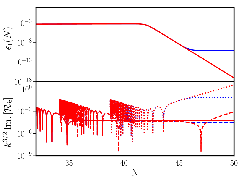
We have worked with the following values for parameters involved in plotting the figure: $\epsilon_{1a}=10^{-4}$, $\epsilon_{2a}=0.05$, $N_{1}=42$, $\Delta N_{1}=0.5$ and $\epsilon_{1b}=10^{-10}$. It should be clear that, while the amplitude of the curvature perturbation grows indefinitely when the ultra slow roll continues, the amplitude freezes when slow roll inflation is restored.

Appendix F The steepest growth of the scalar power spectrum

In models of ultra slow roll and punctuated inflation, we have seen that the scalar power grows rapidly from its COBE normalized values on the CMB scales to higher values at smaller scales over wave numbers that leave the Hubble radius during the transition from slow roll to ultra slow roll. An interesting issue that is worth understanding is the steepest such growth that is possible in models of inflation driven by a single, canonical scalar field. It has been argued that the fastest growth will have $n_{{}_{\mathrm{S}}}-1\simeq 4$ over this range of wave numbers (in this context, see ref. [76]; also see ref. [81]). We find that the reconstructed scenarios RS1 and RS2 easily permit us to examine this issue. Recall that, in these scenarios, the parameter $\Delta N_{1}$ determines the rapidity of the transition from the slow roll to the ultra slow roll regime [cf. eqs. (14)]. We find that it is this parameter that dictates the steepness of the growth in the corresponding scalar power spectra, with smaller $\Delta N_{1}$ producing a faster rise. We have examined the rate of growth in the cases of RS1 and RS2 by varying $\Delta N_{1}$ over a certain range, while keeping the other parameters fixed. In figure 17, we have illustrated the spectra for four values of $\Delta N_{1}$ which are relatively smaller than those we had used for the reconstructions discussed earlier.

Figure 17: The scalar power spectra around the region where they exhibit the sharpest growth have been plotted in the cases of RS1 (on the left) and RS2 (on the right) for a set of values of $\Delta N_{1}$. We have plotted the spectra for the following four values of $\Delta N_{1}$: $(0.1,0.08,0.05,0.01)$ (in red, blue, green and purple, respectively). The insets illustrate the corresponding spectral indices $n_{{}_{\mathrm{S}}}-1$. We have also indicated the $k^{4}$ behavior in the case of RS1 (as dotted lines of corresponding colors on the left) to show how well it matches the spectra during the growth. It should be evident that, while RS1 leads to a growth corresponding to $n_{{}_{\mathrm{S}}}-1\simeq 4$, RS2 permits a steeper but non-uniform growth with $n_{{}_{\mathrm{S}}}-1$ varying between $4$ and $6$ over the relevant wave numbers.

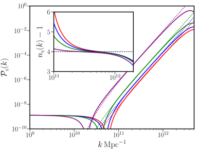
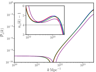
It should be clear from the figure that, in the case of RS1, the rise is fairly steady as the value of $\Delta N_{1}$ is made smaller, with $n_{{}_{\mathrm{S}}}-1\simeq 4$ over the growing regime. In the case of RS2, we find that $n_{{}_{\mathrm{S}}}-1$ varies between $4$ and $6$ over the growing regime and therefore corresponds to a steeper but non-uniform growth of the spectra.

References

- Abbott et al. [2016a] B. Abbott et al. (LIGO Scientific, Virgo), Phys. Rev. Lett. 116, 131103 (2016a), arXiv:1602.03838 [gr-qc] .
- Abbott et al. [2016b] B. Abbott et al. (LIGO Scientific, Virgo), Phys. Rev. D 93, 122003 (2016b), arXiv:1602.03839 [gr-qc] .
- Abbott et al. [2016c] B. Abbott et al. (LIGO Scientific, Virgo), Phys. Rev. Lett. 116, 241102 (2016c), arXiv:1602.03840 [gr-qc] .
- Abbott et al. [2016d] B. P. Abbott et al. (LIGO Scientific, Virgo), Phys. Rev. Lett. 116, 061102 (2016d), arXiv:1602.03837 [gr-qc] .
- Abbott et al. [2016e] B. P. Abbott et al. (LIGO Scientific, Virgo), Phys. Rev. Lett. 116, 241103 (2016e), arXiv:1606.04855 [gr-qc] .
- Abbott et al. [2017a] B. P. Abbott et al. (LIGO Scientific, VIRGO), Phys. Rev. Lett. 118, 221101 (2017a), [Erratum: Phys. Rev. Lett.121,no.12,129901(2018)], arXiv:1706.01812 [gr-qc] .
- Abbott et al. [2017b] B. P. Abbott et al. (LIGO Scientific, Virgo), Astrophys. J. Lett. 851, L35 (2017b), arXiv:1711.05578 [astro-ph.HE] .
- Abbott et al. [2017c] B. P. Abbott et al. (LIGO Scientific, Virgo), Phys. Rev. Lett. 119, 141101 (2017c), arXiv:1709.09660 [gr-qc] .
- Abbott et al. [2017d] B. P. Abbott et al. (LIGO Scientific, Virgo), Phys. Rev. Lett. 119, 161101 (2017d), arXiv:1710.05832 [gr-qc] .
- Abbott et al. [2020a] R. Abbott et al. (LIGO Scientific, Virgo), (2020a), arXiv:2004.08342 [astro-ph.HE] .
- Abbott et al. [2020b] B. P. Abbott et al. (LIGO Scientific, Virgo), Astrophys. J. Lett. 892, L3 (2020b), arXiv:2001.01761 [astro-ph.HE] .
- Abbott et al. [2020c] R. Abbott et al. (LIGO Scientific, Virgo), Astrophys. J. 896, L44 (2020c), arXiv:2006.12611 [astro-ph.HE] .
- De Luca et al. [2020] V. De Luca, G. Franciolini, P. Pani, and A. Riotto, JCAP 06, 044, arXiv:2005.05641 [astro-ph.CO] .
- Jedamzik [2020a] K. Jedamzik, (2020a), arXiv:2006.11172 [astro-ph.CO] .
- Jedamzik [2020b] K. Jedamzik, (2020b), arXiv:2007.03565 [astro-ph.CO] .
- Carr [1975] B. J. Carr, Astrophys. J. 201, 1 (1975).
- Carr et al. [2010] B. J. Carr, K. Kohri, Y. Sendouda, and J. Yokoyama, Phys. Rev. D81, 104019 (2010), arXiv:0912.5297 [astro-ph.CO] .
- Carr et al. [2016] B. Carr, F. Kuhnel, and M. Sandstad, Phys. Rev. D 94, 083504 (2016), arXiv:1607.06077 [astro-ph.CO] .
- Carr and Silk [2018] B. Carr and J. Silk, Mon. Not. Roy. Astron. Soc. 478, 3756 (2018), arXiv:1801.00672 [astro-ph.CO] .
- Sasaki et al. [2018] M. Sasaki, T. Suyama, T. Tanaka, and S. Yokoyama, Class. Quant. Grav. 35, 063001 (2018), arXiv:1801.05235 [astro-ph.CO] .
- Carr and Kuhnel [2020] B. Carr and F. Kuhnel, (2020), arXiv:2006.02838 [astro-ph.CO] .
- Chongchitnan and Efstathiou [2007] S. Chongchitnan and G. Efstathiou, JCAP 01, 011, arXiv:astro-ph/0611818 .
- Ade et al. [2016a] P. Ade et al. (Planck), Astron. Astrophys. 594, A20 (2016a), arXiv:1502.02114 [astro-ph.CO] .
- Akrami et al. [2018] Y. Akrami et al. (Planck), (2018), arXiv:1807.06211 [astro-ph.CO] .
- Garcia-Bellido and Ruiz Morales [2017] J. Garcia-Bellido and E. Ruiz Morales, Phys. Dark Univ. 18, 47 (2017), arXiv:1702.03901 [astro-ph.CO] .
- Ballesteros and Taoso [2018] G. Ballesteros and M. Taoso, Phys. Rev. D 97, 023501 (2018), arXiv:1709.05565 [hep-ph] .
- Germani and Prokopec [2017] C. Germani and T. Prokopec, Phys. Dark Univ. 18, 6 (2017), arXiv:1706.04226 [astro-ph.CO] .
- Dalianis et al. [2019] I. Dalianis, A. Kehagias, and G. Tringas, JCAP 01, 037, arXiv:1805.09483 [astro-ph.CO] .
- Bhaumik and Jain [2019] N. Bhaumik and R. K. Jain 10.1088/1475-7516/2020/01/037 (2019), [JCAP2001,037(2020)], arXiv:1907.04125 [astro-ph.CO] .
- Roberts et al. [1995] D. Roberts, A. R. Liddle, and D. H. Lyth, Phys. Rev. D 51, 4122 (1995), arXiv:astro-ph/9411104 .
- Leach and Liddle [2001] S. M. Leach and A. R. Liddle, Phys. Rev. D63, 043508 (2001), arXiv:astro-ph/0010082 [astro-ph] .
- Leach et al. [2001] S. M. Leach, M. Sasaki, D. Wands, and A. R. Liddle, Phys. Rev. D 64, 023512 (2001), arXiv:astro-ph/0101406 .
- Jain et al. [2007] R. K. Jain, P. Chingangbam, and L. Sriramkumar, JCAP 10, 003, arXiv:astro-ph/0703762 .
- Jain et al. [2009] R. K. Jain, P. Chingangbam, J.-O. Gong, L. Sriramkumar, and T. Souradeep, JCAP 01, 009, arXiv:0809.3915 [astro-ph] .
- Jain et al. [2010] R. K. Jain, P. Chingangbam, L. Sriramkumar, and T. Souradeep, Phys. Rev. D 82, 023509 (2010), arXiv:0904.2518 [astro-ph.CO] .
- Ragavendra et al. [2020] H. Ragavendra, D. Chowdhury, and L. Sriramkumar, (2020), arXiv:2003.01099 [astro-ph.CO] .
- Kannike et al. [2017] K. Kannike, L. Marzola, M. Raidal, and H. Veermäe, JCAP 09, 020, arXiv:1705.06225 [astro-ph.CO] .
- Ananda et al. [2007] K. N. Ananda, C. Clarkson, and D. Wands, Phys. Rev. D75, 123518 (2007), arXiv:gr-qc/0612013 [gr-qc] .
- Baumann et al. [2007] D. Baumann, P. J. Steinhardt, K. Takahashi, and K. Ichiki, Phys. Rev. D76, 084019 (2007), arXiv:hep-th/0703290 [hep-th] .
- Saito and Yokoyama [2009] R. Saito and J. Yokoyama, Phys. Rev. Lett. 102, 161101 (2009), [Erratum: Phys.Rev.Lett. 107, 069901 (2011)], arXiv:0812.4339 [astro-ph] .
- Saito and Yokoyama [2010] R. Saito and J. Yokoyama, Prog. Theor. Phys. 123, 867 (2010), [Erratum: Prog.Theor.Phys. 126, 351–352 (2011)], arXiv:0912.5317 [astro-ph.CO] .
- Kohri and Terada [2018] K. Kohri and T. Terada, Phys. Rev. D 97, 123532 (2018), arXiv:1804.08577 [gr-qc] .
- Espinosa et al. [2018] J. R. Espinosa, D. Racco, and A. Riotto, JCAP 1809, 012, arXiv:1804.07732 [hep-ph] .
- Pi and Sasaki [2020] S. Pi and M. Sasaki, (2020), arXiv:2005.12306 [gr-qc] .
- Abbott et al. [2017e] B. P. Abbott et al. (LIGO Scientific, Virgo), Phys. Rev. Lett. 118, 121101 (2017e), [Erratum: Phys.Rev.Lett. 119, 029901 (2017)], arXiv:1612.02029 [gr-qc] .
- Sazhin [1977] M. V. Sazhin, Vestn. Mosk. Univ. Fiz. Astron. 18, 82 (1977).
- Detweiler [1979] S. L. Detweiler, Astrophys. J. 234, 1100 (1979).
- Arzoumanian et al. [2018] Z. Arzoumanian et al. (NANOGRAV), Astrophys. J. 859, 47 (2018), arXiv:1801.02617 [astro-ph.HE] .
- Amaro-Seoane et al. [2017] P. Amaro-Seoane et al. (LISA), (2017), arXiv:1702.00786 [astro-ph.IM] .
- Barausse et al. [2020] E. Barausse et al. 10.1007/s10714-020-02691-1. (2020), arXiv:2001.09793 [gr-qc] .
- Crowder and Cornish [2005] J. Crowder and N. J. Cornish, Phys. Rev. D72, 083005 (2005), arXiv:gr-qc/0506015 [gr-qc] .
- Corbin and Cornish [2006] V. Corbin and N. J. Cornish, Class. Quant. Grav. 23, 2435 (2006), arXiv:gr-qc/0512039 [gr-qc] .
- Baker et al. [2019] J. Baker et al., (2019), arXiv:1907.11305 [astro-ph.IM] .
- Kawamura et al. [2011] S. Kawamura et al., Laser interferometer space antenna. Proceedings, 8th International LISA Symposium, Stanford, USA, June 28-July 2, 2010, Class. Quant. Grav. 28, 094011 (2011).
- Kawamura [2019] S. Kawamura (DECIGO working group), PoS KMI2019, 019 (2019).
- Punturo et al. [2010] M. Punturo et al., Proceedings, 14th Workshop on Gravitational wave data analysis (GWDAW-14): Rome, Italy, January 26-29, 2010, Class. Quant. Grav. 27, 194002 (2010).
- Sathyaprakash et al. [2012] B. Sathyaprakash et al., Gravitational waves. Numerical relativity - data analysis. Proceedings, 9th Edoardo Amaldi Conference, Amaldi 9, and meeting, NRDA 2011, Cardiff, UK, July 10-15, 2011, Class. Quant. Grav. 29, 124013 (2012), [Erratum: Class. Quant. Grav.30,079501(2013)], arXiv:1206.0331 [gr-qc] .
- Chen et al. [2008] X. Chen, R. Easther, and E. A. Lim, JCAP 04, 010, arXiv:0801.3295 [astro-ph] .
- Martin and Sriramkumar [2012] J. Martin and L. Sriramkumar, JCAP 01, 008, arXiv:1109.5838 [astro-ph.CO] .
- Hazra et al. [2013] D. K. Hazra, L. Sriramkumar, and J. Martin, JCAP 05, 026, arXiv:1201.0926 [astro-ph.CO] .
- Seery and Hidalgo [2006] D. Seery and J. Hidalgo, JCAP 07, 008, arXiv:astro-ph/0604579 .
- Hidalgo [2007] J. Hidalgo, (2007), arXiv:0708.3875 [astro-ph] .
- Motohashi and Hu [2017] H. Motohashi and W. Hu, Phys. Rev. D96, 063503 (2017), arXiv:1706.06784 [astro-ph.CO] .
- Atal and Germani [2019] V. Atal and C. Germani, Phys. Dark Univ. 24, 100275 (2019), arXiv:1811.07857 [astro-ph.CO] .
- Franciolini et al. [2018] G. Franciolini, A. Kehagias, S. Matarrese, and A. Riotto, JCAP 03, 016, arXiv:1801.09415 [astro-ph.CO] .
- Kehagias et al. [2019] A. Kehagias, I. Musco, and A. Riotto, JCAP 12, 029, arXiv:1906.07135 [astro-ph.CO] .
- Atal et al. [2020] V. Atal, J. Cid, A. Escrivà, and J. Garriga, JCAP 05, 022, arXiv:1908.11357 [astro-ph.CO] .
- De Luca et al. [2019] V. De Luca, G. Franciolini, A. Kehagias, M. Peloso, A. Riotto, and C. Ünal, JCAP 07, 048, arXiv:1904.00970 [astro-ph.CO] .
- Passaglia et al. [2019] S. Passaglia, W. Hu, and H. Motohashi, Phys. Rev. D 99, 043536 (2019), arXiv:1812.08243 [astro-ph.CO] .
- Ezquiaga et al. [2020] J. M. Ezquiaga, J. García-Bellido, and V. Vennin, JCAP 03, 029, arXiv:1912.05399 [astro-ph.CO] .
- Cai et al. [2019a] R.-g. Cai, S. Pi, and M. Sasaki, Phys. Rev. Lett. 122, 201101 (2019a), arXiv:1810.11000 [astro-ph.CO] .
- Unal [2019] C. Unal, Phys. Rev. D 99, 041301 (2019), arXiv:1811.09151 [astro-ph.CO] .
- Cai et al. [2019b] R.-G. Cai, S. Pi, S.-J. Wang, and X.-Y. Yang 10.1088/1475-7516/2019/10/059 (2019b), [JCAP1910,059(2019)], arXiv:1907.06372 [astro-ph.CO] .
- Yuan and Huang [2020] C. Yuan and Q.-G. Huang, (2020), arXiv:2007.10686 [astro-ph.CO] .
- Hertzberg and Yamada [2018] M. P. Hertzberg and M. Yamada, Phys. Rev. D97, 083509 (2018), arXiv:1712.09750 [astro-ph.CO] .
- Byrnes et al. [2019] C. T. Byrnes, P. S. Cole, and S. P. Patil, JCAP 06, 028, arXiv:1811.11158 [astro-ph.CO] .
- Motohashi et al. [2020] H. Motohashi, S. Mukohyama, and M. Oliosi, JCAP 03, 002, arXiv:1910.13235 [gr-qc] .
- Allahverdi et al. [2007] R. Allahverdi, K. Enqvist, J. Garcia-Bellido, A. Jokinen, and A. Mazumdar, JCAP 06, 019, arXiv:hep-ph/0610134 .
- Dalianis and Kritos [2020] I. Dalianis and K. Kritos, (2020), arXiv:2007.07915 [astro-ph.CO] .
- Özsoy et al. [2018] O. Özsoy, S. Parameswaran, G. Tasinato, and I. Zavala, JCAP 1807, 005, arXiv:1803.07626 [hep-th] .
- Özsoy and Tasinato [2020] O. Özsoy and G. Tasinato, JCAP 04, 048, arXiv:1912.01061 [astro-ph.CO] .
- Gordon et al. [2000] C. Gordon, D. Wands, B. A. Bassett, and R. Maartens, Phys. Rev. D 63, 023506 (2000), arXiv:astro-ph/0009131 .
- Unnikrishnan and Sriramkumar [2010] S. Unnikrishnan and L. Sriramkumar, Phys. Rev. D 81, 103511 (2010), arXiv:1002.0820 [astro-ph.CO] .
- Cicoli et al. [2018] M. Cicoli, V. A. Diaz, and F. G. Pedro, JCAP 1806 (06), 034, arXiv:1803.02837 [hep-th] .
- Pi et al. [2019] S. Pi, M. Sasaki, and Y.-l. Zhang, JCAP 06, 049, arXiv:1904.06304 [gr-qc] .
- D’Amico and Kaloper [2020] G. D’Amico and N. Kaloper, (2020), arXiv:2011.09489 [hep-th] .
- Tasinato [2020] G. Tasinato, (2020), arXiv:2012.02518 [hep-th] .
- Green et al. [2004] A. M. Green, A. R. Liddle, K. A. Malik, and M. Sasaki, Phys. Rev. D70, 041502 (2004), arXiv:astro-ph/0403181 [astro-ph] .
- Germani and Musco [2019] C. Germani and I. Musco, Phys. Rev. Lett. 122, 141302 (2019), arXiv:1805.04087 [astro-ph.CO] .
- Germani and Sheth [2020] C. Germani and R. K. Sheth, Phys. Rev. D 101, 063520 (2020), arXiv:1912.07072 [astro-ph.CO] .
- Escrivà [2020] A. Escrivà, Phys. Dark Univ. 27, 100466 (2020), arXiv:1907.13065 [gr-qc] .
- Escrivà et al. [2020a] A. Escrivà, C. Germani, and R. K. Sheth, Phys. Rev. D 101, 044022 (2020a), arXiv:1907.13311 [gr-qc] .
- Escrivà et al. [2020b] A. Escrivà, C. Germani, and R. K. Sheth, (2020b), arXiv:2007.05564 [gr-qc] .
- Ade et al. [2016b] P. Ade et al. (Planck), Astron. Astrophys. 594, A13 (2016b), arXiv:1502.01589 [astro-ph.CO] .
- Aghanim et al. [2018] N. Aghanim et al. (Planck), (2018), arXiv:1807.06209 [astro-ph.CO] .
- Barnacka et al. [2012] A. Barnacka, J. F. Glicenstein, and R. Moderski, Phys. Rev. D86, 043001 (2012), arXiv:1204.2056 [astro-ph.CO] .
- Katz et al. [2018] A. Katz, J. Kopp, S. Sibiryakov, and W. Xue, JCAP 1812, 005, arXiv:1807.11495 [astro-ph.CO] .
- Griest et al. [2013] K. Griest, A. M. Cieplak, and M. J. Lehner, Phys. Rev. Lett. 111, 181302 (2013).
- Allsman et al. [2001] R. Allsman et al. (Macho), Astrophys. J. Lett. 550, L169 (2001), arXiv:astro-ph/0011506 .
- Tisserand et al. [2007] P. Tisserand et al. (EROS-2), Astron. Astrophys. 469, 387 (2007), arXiv:astro-ph/0607207 [astro-ph] .
- Wyrzykowski et al. [2011] L. Wyrzykowski et al., Mon. Not. Roy. Astron. Soc. 416, 2949 (2011), arXiv:1106.2925 [astro-ph.GA] .
- Ricotti et al. [2008] M. Ricotti, J. P. Ostriker, and K. J. Mack, Astrophys. J. 680, 829 (2008), arXiv:0709.0524 [astro-ph] .
- Brandt [2016] T. D. Brandt, Astrophys. J. 824, L31 (2016), arXiv:1605.03665 [astro-ph.GA] .
- Carr et al. [2020] B. Carr, K. Kohri, Y. Sendouda, and J. Yokoyama, (2020), arXiv:2002.12778 [astro-ph.CO] .
- Green and Kavanagh [2020] A. M. Green and B. J. Kavanagh, (2020), arXiv:2007.10722 [astro-ph.CO] .
- Montero-Camacho et al. [2019] P. Montero-Camacho, X. Fang, G. Vasquez, M. Silva, and C. M. Hirata, JCAP 1908, 031, arXiv:1906.05950 [astro-ph.CO] .
- Laha [2019] R. Laha, Phys. Rev. Lett. 123, 251101 (2019), arXiv:1906.09994 [astro-ph.HE] .
- Dasgupta et al. [2020] B. Dasgupta, R. Laha, and A. Ray, Phys. Rev. Lett. 125, 101101 (2020), arXiv:1912.01014 [hep-ph] .
- Laha et al. [2020] R. Laha, J. B. Muñoz, and T. R. Slatyer, Phys. Rev. D 101, 123514 (2020), arXiv:2004.00627 [astro-ph.CO] .
- Maggiore [2000] M. Maggiore, Phys. Rept. 331, 283 (2000), arXiv:gr-qc/9909001 .
- Bartolo et al. [2016] N. Bartolo et al., JCAP 12, 026, arXiv:1610.06481 [astro-ph.CO] .
- Bartolo et al. [2019a] N. Bartolo, V. De Luca, G. Franciolini, A. Lewis, M. Peloso, and A. Riotto, Phys. Rev. Lett. 122, 211301 (2019a), arXiv:1810.12218 [astro-ph.CO] .
- Bartolo et al. [2019b] N. Bartolo, V. De Luca, G. Franciolini, M. Peloso, D. Racco, and A. Riotto, Phys. Rev. D 99, 103521 (2019b), arXiv:1810.12224 [astro-ph.CO] .
- Moore et al. [2015] C. Moore, R. Cole, and C. Berry, Class. Quant. Grav. 32, 015014 (2015), arXiv:1408.0740 [gr-qc] .
- Coleman [2019] J. Coleman (MAGIS-100), PoS ICHEP2018, 021 (2019), arXiv:1812.00482 [physics.ins-det] .
- Abbott et al. [2019] B. Abbott et al. (LIGO Scientific, Virgo), Phys. Rev. D 100, 061101 (2019), arXiv:1903.02886 [gr-qc] .
- Abbott et al. [2017f] B. P. Abbott et al. (LIGO Scientific), Class. Quant. Grav. 34, 044001 (2017f), arXiv:1607.08697 [astro-ph.IM] .
- Thrane and Romano [2013] E. Thrane and J. D. Romano, Phys. Rev. D 88, 124032 (2013), arXiv:1310.5300 [astro-ph.IM] .
- Abbott et al. [2009] B. Abbott et al. (LIGO Scientific, VIRGO), Nature 460, 990 (2009), arXiv:0910.5772 [astro-ph.CO] .
- Tsuneto et al. [2019] M. Tsuneto, A. Ito, T. Noumi, and J. Soda, JCAP 03, 032, arXiv:1812.10615 [gr-qc] .
- Powell and Tasinato [2020] C. Powell and G. Tasinato, JCAP 01, 017, arXiv:1910.04758 [gr-qc] .
- Iacconi et al. [2020] L. Iacconi, M. Fasiello, H. Assadullahi, and D. Wands, JCAP 12, 005, arXiv:2008.00452 [astro-ph.CO] .
- Ade et al. [2016c] P. Ade et al. (Planck), Astron. Astrophys. 594, A17 (2016c), arXiv:1502.01592 [astro-ph.CO] .
- Akrami et al. [2019] Y. Akrami et al. (Planck), (2019), arXiv:1905.05697 [astro-ph.CO] .
- Maldacena [2003] J. M. Maldacena, JHEP 05, 013, arXiv:astro-ph/0210603 .
- Seery and Lidsey [2005] D. Seery and J. E. Lidsey, JCAP 06, 003, arXiv:astro-ph/0503692 .
- Chen [2010] X. Chen, Adv. Astron. 2010, 638979 (2010), arXiv:1002.1416 [astro-ph.CO] .
- Arroja and Tanaka [2011] F. Arroja and T. Tanaka, JCAP 05, 005, arXiv:1103.1102 [astro-ph.CO] .
- Komatsu [2010] E. Komatsu, Class. Quant. Grav. 27, 124010 (2010), arXiv:1003.6097 [astro-ph.CO] .
- Creminelli and Zaldarriaga [2004] P. Creminelli and M. Zaldarriaga, JCAP 10, 006, arXiv:astro-ph/0407059 .
- Namjoo et al. [2013] M. H. Namjoo, H. Firouzjahi, and M. Sasaki, EPL 101, 39001 (2013), arXiv:1210.3692 [astro-ph.CO] .
- Martin et al. [2013] J. Martin, H. Motohashi, and T. Suyama, Phys. Rev. D 87, 023514 (2013), arXiv:1211.0083 [astro-ph.CO] .
- Motohashi et al. [2015] H. Motohashi, A. A. Starobinsky, and J. Yokoyama, JCAP 09, 018, arXiv:1411.5021 [astro-ph.CO] .
- Sreenath et al. [2015] V. Sreenath, D. K. Hazra, and L. Sriramkumar, JCAP 02, 029, arXiv:1410.0252 [astro-ph.CO] .
- Bravo and Palma [2020] R. Bravo and G. A. Palma, (2020), arXiv:2009.03369 [hep-th] .
- Pajer [2020] E. Pajer, (2020), arXiv:2010.12818 [hep-th] .
- Komatsu and Spergel [2001] E. Komatsu and D. N. Spergel, Phys. Rev. D 63, 063002 (2001), arXiv:astro-ph/0005036 .
- Byrnes et al. [2012] C. T. Byrnes, E. J. Copeland, and A. M. Green, Phys. Rev. D86, 043512 (2012), arXiv:1206.4188 [astro-ph.CO] .
- Taoso and Urbano [2021] M. Taoso and A. Urbano, (2021), arXiv:2102.03610 [astro-ph.CO] .
- Riccardi et al. [2021] F. Riccardi, M. Taoso, and A. Urbano, (2021), arXiv:2102.04084 [astro-ph.CO] .
- Tada and Vennin [2017] Y. Tada and V. Vennin, JCAP 02, 021, arXiv:1609.08876 [astro-ph.CO] .
- Suyama et al. [2020] T. Suyama, Y. Tada, and M. Yamaguchi, (2020), arXiv:2008.13364 [astro-ph.CO] .
- Matarrese et al. [2020] S. Matarrese, L. Pilo, and R. Rollo, (2020), arXiv:2007.08877 [astro-ph.CO] .
- Mishra and Sahni [2020] S. S. Mishra and V. Sahni, JCAP 04, 007, arXiv:1911.00057 [gr-qc] .
- Cai et al. [2019c] R.-G. Cai, S. Pi, S.-J. Wang, and X.-Y. Yang, JCAP 05, 013, arXiv:1901.10152 [astro-ph.CO] .
- Cai et al. [2020] R.-G. Cai, Z.-K. Guo, J. Liu, L. Liu, and X.-Y. Yang, JCAP 06, 013, arXiv:1912.10437 [astro-ph.CO] .
- Ashoorioon et al. [2019] A. Ashoorioon, A. Rostami, and J. T. Firouzjaee, (2019), arXiv:1912.13326 [astro-ph.CO] .
- Lin et al. [2020] J. Lin, Q. Gao, Y. Gong, Y. Lu, C. Zhang, and F. Zhang, Phys. Rev. D 101, 103515 (2020), arXiv:2001.05909 [gr-qc] .
- Yi et al. [2020] Z. Yi, Y. Gong, B. Wang, and Z.-h. Zhu, (2020), arXiv:2007.09957 [gr-qc] .
- Palma et al. [2020] G. A. Palma, S. Sypsas, and C. Zenteno, (2020), arXiv:2004.06106 [astro-ph.CO] .
- Fumagalli et al. [2020] J. Fumagalli, S. Renaux-Petel, J. W. Ronayne, and L. T. Witkowski, (2020), arXiv:2004.08369 [hep-th] .
- Braglia et al. [2020] M. Braglia, D. K. Hazra, F. Finelli, G. F. Smoot, L. Sriramkumar, and A. A. Starobinsky, JCAP 08, 001, arXiv:2005.02895 [astro-ph.CO] .