A(DP)²SGD: Asynchronous Decentralized Parallel Stochastic Gradient Descent with Differential Privacy

Abstract

As deep learning models are usually massive and complex, distributed learning is essential for increasing training efficiency. Moreover, in many real-world application scenarios like healthcare, distributed learning can also keep the data local and protect privacy. A popular distributed learning strategy is federated learning, where there is a central server storing the global model and a set of local computing nodes updating the model parameters with their corresponding data. The updated model parameters will be processed and transmitted to the central server, which leads to heavy communication costs. Recently, asynchronous decentralized distributed learning has been proposed and demonstrated to be a more efficient and practical strategy where there is no central server, so that each computing node only communicates with its neighbors. Although no raw data will be transmitted across different local nodes, there is still a risk of information leak during the communication process for malicious participants to make attacks. In this paper, we present a differentially private version of asynchronous decentralized parallel SGD (ADPSGD) framework, or A(DP)²SGD for short, which maintains communication efficiency of ADPSGD and prevents the inference from malicious participants. Specifically, Rényi differential privacy is used to provide tighter privacy analysis for our composite Gaussian mechanisms while the convergence rate is consistent with the non-private version. Theoretical analysis shows A(DP)²SGD also converges at the optimal $\mathcal{O}(1/\sqrt{T})$ rate as SGD. Empirically, A(DP)²SGD achieves comparable model accuracy as the differentially private version of Synchronous SGD (SSGD) but runs much faster than SSGD in heterogeneous computing environments.

1 Introduction

Distributed Deep Learning (DDL), as a collaborative modeling mechanism that could save storage cost and increase computing efficiency when carrying out machine learning tasks, has demonstrated strong potentials in various areas, especially for training large deep learning models on large dataset such as ImageNet akiba2017chainermn ; zhang2015staleness ; you2017imagenet . Typically, assume there are $K$ workers where the data reside (a worker could be a machine or a GPU, etc), distributed machine learning problem boils down to solving an empirical risk minimization problem of the form:

$$\min_{\mathbf{w}\in\mathbb{R}^{d}}F(\mathbf{w}):=\mathbb{E}_{k\sim{\mathcal{I}}}[F_{k}(\mathbf{w})]=\sum_{k=1}^{K}p_{k}F_{k}(\mathbf{w}),$$ (1)

where $p_{k}$’s define a distribution, that is, $p_{k}\geq 0$ and $\sum_{k}p_{k}=1$, and $p_{k}$ indicates the percentage of the updates performed by worker $k$. The objective $F(\mathbf{w})$ in problem (1) can be rephrased as a linear combination of the local empirical objectives $F_{k}(\mathbf{w}):=\mathbb{E}_{\xi\sim{\mathcal{D}_{k}}}[f(\mathbf{w};\xi)]$, where $\mathcal{D}_{k}$ denotes the data distribution associated to worker $k\in[K]$ and $\xi$ is a data point sampled via $\mathcal{D}_{k}$.

In particular, algorithms for DDL face with following issues. On one hand, the communication cost to the central server may not be affordable since a large number of updates of a number of workers are usually involved. Many practical peer-to-peer networks are usually dynamic, and it is not possible to regularly access a fixed central server. Moreover, because of the dependency on the central server, all workers are required to agree on one trusted central body, and whose failure would interrupt the entire training process for all workers. Therefore, researchers have started to study fully decentralized framework where the central server is not required shayan2018biscotti ; roy2019braintorrent ; Lalitha2019decentralized ; lalitha2019peer , which is also the focus of this paper. In addition, to improve flexibility and scalability, as in lian2018asynchronous , we consider the asynchronous communication where the participant workers do not operate in the lock-step.

On the other hand, since a large number of workers usually participate in the training process in distributed learning, it is difficult to ensure none of them are malicious. Despite no raw data sharing and no central body are required to coordinate the training process of the global model, the open computing network architecture and extensive collaborations among works still inevitably provide the opportunities for malicious worker to infer the private information about another worker given the execution of $f(\mathbf{w})$, or over the shared predictive model $\mathbf{w}$ truex2018hybrid . To alleviate this issue, differential privacy (DP), as an alternative theoretical model to provide mathematical privacy guarantees, has caught people’s attention dwork2006our . DP ensures that the addition or removal of a single data sample does not substantially affect the outcome of any analysis, thus is widely applied to many algorithms to prevent implicit leakage, not only for traditional algorithms, e.g. principal component analysis chaudhuri2013near , support vector machine rubinstein2009learning , but also for modern deep learning research abadi2016deep ; mcmahan2017learning .

In this paper, we focus on achieving differential privacy in asynchronous decentralized communication setting, where we target to obtain a good convergence rate while keeping the communication cost low. We highlight the following aspects of our contributions:

• We propose a differentially private version of ADPSGD, i.e., A(DP)²SGD, where differential privacy is introduced to protect the frequently exchanged variables.

• We present the privacy and utility guarantees for A(DP)²SGD, where Rényi differential privacy is introduced to provide tighter privacy analysis of composite heterogeneous mechanisms mironov2017renyi while the convergence rate is consistent with the non-private version.

• Empirically, we conduct experiments on both computer vision (CIFAR-10) and speech recognition (SWB300) datasets. A(DP)²SGD achieves comparable model accuracy and level of DP protection as differentially private version of Synchronous SGD (SSGD) and runs much faster than SSGD in heterogeneous computing environments.

2 Related Work

2.1 Differential Privacy

Differential privacy (DP), first introduced by Dwork et al. dwork2006our , is a mathematical definition for the privacy loss associated with any data release drawn from a statistical database. The basic property of DP mechanism is that the change of the output probability distribution is limited when the input of the algorithm is slightly disturbed. Formally, it says:

Definition 1 (($\epsilon,\delta$)-DP dwork2006our ).

A randomized mechanism $\mathcal{M}:\mathcal{X}^{n}\to\mathcal{R}$ satisfies ($\epsilon,\delta$)-differential privacy, or ($\epsilon,\delta$)-DP for short, if for all $\mathbf{x},\mathbf{x}^{\prime}\in\mathcal{X}^{n}$ differing on a single entry, and for any subset of outputs $S\subseteq\mathcal{R}$, it holds that

$$Pr[\mathcal{M}(\mathbf{x})\in S]\leq e^{\epsilon}Pr[\mathcal{M}(\mathbf{x}^{\prime})\in S]+\delta.$$ (2)

The parameter $\epsilon$ balances the accuracy of the differentially private $\mathcal{M}$ and how much it leaks shokri2015privacy . The presence of a non-zero $\delta$ allows us to relax the strict relative shift in unlikely events dwork2006our .

Although by relaxing the guarantee to ($\epsilon,\delta$)-DP, advanced composition allows tighter analyses for compositions of (pure) differentially private mechanisms ($\delta=0$), iterating this process quickly leads to a combinatorial explosion of parameters mironov2017renyi . To address the shortcomings of ($\epsilon,\delta$)-DP, Mironov et al. mironov2017renyi proposed a natural relaxation of differential privacy based on the Rényi divergence, i.e., Rényi differential privacy (RDP). The new definition RDP shares many important properties with the standard definition of differential privacy, while additionally allowing for a more rigorous analysis of composite heterogeneous mechanisms mironov2017renyi .

2.2 Differentially Private Distributed Learning

Existing literature on differentially private distributed learning either focus on centralized learning or synchronous communication or convex problems. Our work combines decentralized learning, asynchronous communication and non-convex optimization in a DP setting. In contrast, Cheng et al. cheng2018leasgd ; cheng2019towards focus on decentralized learning systems and aim to achieve differential privacy, but their convergence analysis is applied to strongly convex problems only. Bellet et al. bellet2017fast ; bellet2017personalized obtain an efficient and fully decentralized protocol working in an asynchronous fashion by a block coordinate descent algorithm and make it differentially private with Laplace mechanism, but their convergence analysis is only applied to convex problems.

Lu et al. lu2019differentially propose a differentially private asynchronous federated learning scheme for resource sharing in vehicular networks. They perform the convergence boosting by updates verification and weighted aggregation without any theoretical analysis. Li et al. li2019asynchronous aims to secure asynchronous edge-cloud collaborative federated learning with differential privacy. But they choose centralized learning and conduct analysis under the convex condition. In this paper, we focus on achieving differential privacy in asynchronous decentralized communication setting and dealing with non-convex problems.

3 A(DP)²SGD Algorithm

Specifically, the decentralized communication network is modeled via an undirected graph $G=([K],\,\mathcal{E})$, consisting of the set $[K]$ of nodes and the set $\mathcal{E}$ of edges. The set $\mathcal{E}$ are unordered pairs of elements of $[K]$. Node $k\in[K]$ is only connected to a subset of the other nodes, and not necessarily all of them. We allow the information collected at each node to be propagated throughout the network. To improve flexibility and scalability, we consider the asynchronous communication where the participant workers do not operate in a lock-step lian2018asynchronous .

During optimization, each worker maintains a local copy of the optimization variable. Suppose that all local models are initialized with the same initialization, i.e., $\mathbf{w}_{k}^{0}=\mathbf{w}^{0},k=1,...,K$. Let $\mathbf{w}_{k}^{t}$ denote the value at worker $k$ after $t$ iterations. We implement stochastic gradient descent in a decentralized asynchronous manner by the following steps, which are executed in parallel at every worker, $k=1,...,K$:

• Sample data: Sample a mini-batch of training data denoted by $\{\xi_{k}^{i}\}_{i=1}^{B}$ from local memory of worker $k$ with the sampling probability $\frac{B}{n_{k}}$, where $B$ is the batch size.

• Compute gradients: Worker $k$ locally computes the stochastic gradient: $g^{t}(\hat{\mathbf{w}}_{k}^{t};\xi_{k}^{t}):=\sum_{i=1}^{B}\triangledown F_{k}(\hat{\mathbf{w}}_{k}^{t};\xi_{k}^{t,i})$, where $\hat{\mathbf{w}}_{k}^{t}$ is read from the local memory.

• Averaging: Randomly sample a doubly stochastic matrix $\mathbf{A}$ and average local models by:

  $$[\mathbf{w}_{1}^{\prime},\mathbf{w}_{2}^{\prime},...,\mathbf{w}_{K}^{\prime}]\leftarrow[\mathbf{w}_{1},\mathbf{w}_{2},...,\mathbf{w}_{K}]\mathbf{A};$$ (3)

  Note that each worker runs the above process separately without any global synchronization.

• Update model: Worker $k$ locally updates the model:

  $$\mathbf{w}_{k}\leftarrow\mathbf{w}_{k}^{\prime}-\eta g^{t}(\hat{\mathbf{w}}_{k};\xi_{k}),$$ (4)

  Noth that averaging step and update model step can run in parallel. $\hat{\mathbf{w}}_{k}$ may not be the same as $\mathbf{w}^{\prime}_{k}$ since it may be modified by other workers in the last averaging step.

All workers simultaneously run the procedure above.

As we stated, the model is trained locally without revealing the input data or the model’s output to any workers, thus it prevents the direct leakage while training or using the model. However, recall in the averaging step, the model variables exchange frequently during training. In this case, the workers still can infer some information about another worker’s private dataset given the execution over the shared model variables truex2018hybrid . To solve this issue, we apply differential privacy to the exchanged model variables.

The general idea to achieve differential privacy is to add a stochastic component to the variables that need to be protected. In our case, the exchanged information is model variables $\mathbf{w}_{k}$. Note that the computation of $\mathbf{w}_{k}$ depends on the gradients. Thus, instead of adding noise directly on the exchanged model variable $\mathbf{w}_{k}$, we inject the noise on the gradients:

$$\tilde{g}(\hat{\mathbf{w}}_{k};\xi_{k})=g(\hat{\mathbf{w}}_{k};\xi_{k})+\mathbf{n},$$

where $\mathbf{n}\sim\mathcal{N}(0,\sigma^{2}\triangle_{2}^{2}(g))$ is the Gaussian distribution. The global sensitivity estimate $\triangle_{2}(g)$ is expected significantly reduced, resulting in higher accuracy by ensuring the norm of all gradients is bounded for each update - either globally, or locally shokri2015privacy .

Then the update model step (4) turns into: $\mathbf{w}_{k}\leftarrow\mathbf{w}_{k}^{\prime}-\eta\tilde{g}^{t}(\hat{\mathbf{w}}_{k};\xi_{k})$. Differential privacy ensures that the addition or removal of a data sample does not substantially affect the outcome of any analysis. The specific procedures are summarized in Algorithm 1.

Algorithm 1 A(DP)²SGD (logical view)

1:Initialization: Initialize all local models $\{\mathbf{w}_{k}^{0}\}_{k=1}^{K}\in\mathbb{R}^{d}$ with $\mathbf{w}^{0}$, learning rate $\eta$, batch size $B$, privacy budget $(\epsilon,\delta)$, and total number of iterations $T$.

2:Output: $(\epsilon,\delta)$-differentially private local models.

3:for <$t=0,1,...,T-1$> do

4:     Randomly sample a worker $k^{t}$ of the graph $G$ and randomly sample an doubly stochastic averaging matrix $\mathbf{A}_{t}\in\mathbb{R}^{K\times K}$ dependent on $k^{t}$;

5:     Randomly sample a batch $\xi_{k^{t}}^{t}:=(\xi_{k^{t}}^{t,1},\xi_{k^{t}}^{t,2},...,\xi_{k^{t}}^{t,B})\in\mathbb{R}^{d\times B}$ from local data of the $k^{t}$-th worker with the sampling probability $\frac{B}{n_{k^{t}}}$;

6:     Compute stochastic gradient $g^{t}(\hat{\mathbf{w}}_{k^{t}}^{t};\xi_{k^{t}}^{t})$ locally: $g^{t}(\hat{\mathbf{w}}_{k^{t}}^{t};\xi_{k^{t}}^{t}):=\sum_{i=1}^{B}\triangledown F_{k^{t}}(\hat{\mathbf{w}}_{k^{t}}^{t};\xi_{k^{t}}^{t,i})$;

7:     Add noise $\tilde{g}^{t}(\hat{\mathbf{w}}_{k^{t}}^{t};\xi_{k^{t}}^{t})=g^{t}(\hat{\mathbf{w}}_{k^{t}}^{t};\xi_{k^{t}}^{t})+\mathbf{n}$, where $\mathbf{n}\in\mathbb{R}^{d}\sim\mathcal{N}(0,\sigma^{2}\mathbf{I})$ and $\sigma$ is defined in Theorem 2.

8:     Average local models by $[\mathbf{w}_{1}^{t+1/2},\mathbf{w}_{2}^{t+1/2},...,\mathbf{w}_{K}^{t+1/2}]\leftarrow[\mathbf{w}_{1}^{t},\mathbf{w}_{2}^{t},...,\mathbf{w}_{K}^{t}]\mathbf{A}_{t}$;

9:     Update the local model: $\mathbf{w}_{k^{t}}^{t+1}\leftarrow\mathbf{w}_{k^{t}}^{t+1/2}-\eta\tilde{g}^{t}(\hat{\mathbf{w}}_{k^{t}}^{t};\xi_{k^{t}}^{t});\quad\forall j\neq k^{t},\mathbf{w}_{j}^{t+1}\leftarrow\mathbf{w}_{j}^{t+1/2}$.

10:end for

4 Theoretical Analysis

In this section, we present the utility and privacy guarantees for A(DP)²SGD. Rényi differential privacy is introduced to provide tighter privacy analysis of composite heterogeneous mechanisms  mironov2017renyi while the convergence rate is consistent with ADPSGD.

4.1 Utility Guarantee

We make the following assumptions which are commonly used and consistent with the non-private version of ADPSGD mironov2017renyi to present the utility guarantee.

Assumption 1.

Assumptions for stochastic optimization.

• (Unbiased Estimation). $\mathbb{E}_{\xi\sim\mathcal{D}_{k}}[\triangledown f(\mathbf{w};\xi)]=\triangledown F_{k}(\mathbf{w}),\mathbb{E}_{k\sim\mathcal{I}}[\triangledown F_{k}(\mathbf{w})]=\triangledown F(\mathbf{w})$.

• (Bounded Gradient Variance).

  $$\mathbb{E}_{\xi\sim\mathcal{D}_{k}}\|\triangledown f(\mathbf{w};\xi)-\triangledown F_{k}(\mathbf{w})\|^{2}\leq\varsigma^{2},\mathbb{E}_{k\sim\mathcal{I}}\|\triangledown F_{k}(\mathbf{w})-\triangledown F(\mathbf{w})\|^{2}\leq\upsilon^{2}.$$ (5)

Assumption 2.

Assumptions for asynchronous updates.

• (Spectral Gap). There exists a $\rho\in[0,1)$ such that

  $$\max\{|\lambda_{2}(\mathbb{E}[\mathbf{A}_{t}^{\top}\mathbf{A}_{t}])|,|\lambda_{K}(\mathbb{E}[\mathbf{A}_{t}^{\top}\mathbf{A}_{t}])|\}\leq\rho,\forall t,$$ (6)

  where $\lambda_{i}(\cdot)$ denotes the $i$-th largest eigenvalue of a matrix.

• (Independence). All random variables: $k,k^{t},\xi^{t}\in\{0,1,2,...\}$ are independent. Doubly stochastic averaging matrix $\mathbf{A}_{t}\in\mathbb{R}^{K\times K}$ is a random variable dependent on $k^{t}$.

• (Bounded Staleness). Let’s denote $\hat{\mathbf{W}}^{t}=\mathbf{W}^{t-\tau_{t}}$ and there exists a constant $\tau$ such that $\max_{t}\tau_{t}\leq\tau$.

Note that a smaller $\rho$ means faster information propagation in the network, resulting in faster convergence.

Theorem 1.

Suppose all functions $f_{i}(\cdot)$’s are with L-Lipschitz continuous gradients, and each of $K$ workers has dataset $D^{(k)}$ of size $n_{k}$. Under Assumptions 1 and 2, if we choose $C_{1}>0$, $C_{2}\geq 0$ and $C_{3}\leq 1$,

$$\frac{\sum_{t=0}^{T-1}\mathbb{E}\left\|\triangledown F(\theta^{t})\right\|^{2}}{T}\leq\frac{2\left(\mathbb{E}F(\mathbf{w}^{0})-\mathbb{E}F^{*}\right)K}{\eta TB}+\frac{2\eta L}{BK}(\varsigma^{2}B+6\upsilon^{2}B^{2}+d\sigma^{2}),$$

where $\theta^{t}$ denotes the average of all local models at $t$-th iteration, i.e., $\theta^{t}=\frac{1}{K}\sum_{k=1}^{K}\mathbf{w}_{k}^{t}$. And $C_{1},C_{2},C_{3}$ are respectively defined as

$$C_{1}:= 1-24\eta^{2}B^{2}L^{2}\left(\tau\frac{K-1}{K}+\bar{\rho}\right),C_{3}:=\frac{1}{2}+\frac{\eta BL\tau^{2}}{K}+\left(6\eta^{2}B^{2}L^{2}+\eta KBL+\frac{12\eta^{3}B^{3}L^{3}\tau^{2}}{K}\right)\frac{2\bar{\rho}}{C_{1}},$$

$$C_{2}:= -\left(\frac{\eta BL^{2}}{K}+\frac{6\eta^{2}B^{2}L^{3}}{K^{2}}+\frac{12\eta^{3}B^{3}L^{4}\tau^{2}}{K^{3}}\right)\frac{4\eta^{2}B^{2}\left(\tau\frac{K-1}{K}+\bar{\rho}\right)}{C_{1}}+\frac{\eta B}{2K}-\frac{\eta^{2}B^{2}L}{K^{2}}-\frac{2\eta^{3}B^{3}L^{2}\tau^{2}}{K^{3}},$$

where $\bar{\rho}=\frac{K-1}{K}\left(\frac{1}{1-\rho}+\frac{2\sqrt{\rho}}{(1-\sqrt{\rho})^{2}}\right)$.

Note that $\theta^{0}=\frac{1}{K}\sum_{k=1}^{K}\mathbf{w}_{k}^{0}=\mathbf{w}^{0}$ and $F^{*}$ denotes the optimal solution to (1). Theorem 1 describes the convergence of the average of all local models. By appropriately choosing the learning rate, we obtain the following proposition.

Proposition 1.

In Theorem 1, if the total number of iterations is sufficiently large, in particular,

$$T\geq L^{2}K^{2}\max\biggr{\{}192\left(\tau\frac{K-1}{K}+\bar{\rho}\right),1024K^{2}\bar{\rho}^{2},\frac{64\tau^{2}}{K^{2}},\frac{(K-1)^{1/2}}{K^{1/6}}\left(8\sqrt{6}\tau^{2/3}+8\right)^{2}\left(\tau+\bar{\rho}\frac{K}{K-1}\right)^{2/3}\biggr{\}},$$

and we choose learning rate $\eta=\frac{K}{B\sqrt{T}}$, then we obtain the following convergence rate

$$\frac{\sum_{t=0}^{T-1}\mathbb{E}\left\|\triangledown F(\theta^{t})\right\|^{2}}{T}\leq\frac{2(F(\mathbf{w}^{0})-F^{*})+2L(\varsigma^{2}/B+6\upsilon^{2}+d\sigma^{2}/B^{2})}{\sqrt{T}}.$$

Proposition 1 indicates that if the total number of iterations is sufficiently large, the convergence rate of A(DP)²SGD is $\mathcal{O}(1/\sqrt{T})$ which is consistent with the convergence rate of ADPSGD. This observation indicates that the differentially private version inherits the strengths of ADPSGD.

4.2 Privacy Guarantee

Theorem 2 (Privacy Guarantee).

Suppose all functions $f_{i}(\cdot)$’s are $G$-Lipschitz and each of $K$ workers has dataset $D^{(k)}$ of size $n_{k}$. Given the total number of iterations $T$, for any $\delta>0$ and privacy budget $\epsilon\leq 10B^{2}T\alpha/(3K^{2}n_{(1)}^{2}\mu)$, A(DP)²SGD with injected Gaussian noise $\mathcal{N}(0,\sigma^{2}\mathbf{I})$ is $(\epsilon,\delta)$-differentially private with $\sigma^{2}=20G^{2}T\alpha/(K^{2}n_{(1)}^{2}\mu\epsilon)$, where $\alpha=\log(1/\delta)/((1-\mu)\epsilon)+1$, if there exits $\mu\in(0,1)$ such that

$$\alpha\leq\log\left(\frac{K^{3}n_{(1)}^{3}\mu\epsilon}{K^{2}n_{(1)}^{2}\mu\epsilon B+5T\alpha B^{3}}\right),$$ (7)

where $n_{(1)}$ is the size of the smallest dataset among the $K$ workers.

Additionally, we observe that differential privacy is also guaranteed for each intermediate model estimator of each worker:

Remark 1.

At each iteration $t\in[T]$, intermediate model estimator $\mathbf{w}_{k}^{t}$ is $(\sqrt{t/T}\epsilon,\delta)$-differentially private, $k\in[K]$.

Recall Theorem 1, the difference of introducing Gaussian mechanism lies on the term $2L(d\sigma^{2}/B^{2})/\sqrt{T}$ compared to ADPSGD. The Gaussian noise injected in each iteration is proportional to the total number of iterations. That is, to achieve differential privacy, we need to pay for a constant term which is proportional to the added noise at each iteration. By assuming all functions $f_{i}(\cdot)$’s are with G-Lipschitz and plugging the noise level into the Proposition 1, we obtain the following Proposition.

Proposition 2 (Utility Guarantee).

Suppose all functions $f_{i}(\cdot)$’s are G-Lipschitz in Proposition 1. Given $\epsilon,\delta>0$, under the same conditions of Theorem 2, if the number of iterations $T$ further satisfies

$$T=\frac{2\left(F(\mathbf{w}^{0})-F^{*}+L(\varsigma^{2}/B+6\upsilon^{2})\right)K^{2}n_{(1)}^{2}\epsilon^{2}}{40dLG^{2}\log(1/\delta)},$$ (8)

let $C_{4}=4\sqrt{5}\left(1+\frac{1}{B^{2}\mu(1-\mu)}\right)$, then A(DP)²SGD’s output $\tilde{\theta}=\sum_{t=1}^{T}\theta^{t}$ satisfies

$$\mathbb{E}\left\|\triangledown F(\tilde{\theta})\right\|^{2}\leq C_{4}\frac{G\sqrt{dL\left(F(\mathbf{w}^{0})-F^{*}+L(\varsigma^{2}/B+6\upsilon^{2})\right)\log(1/\delta)}}{Kn_{(1)}\epsilon}.$$

5 Experiments

We implement Synchronous SGD (SYNC) as the "golden" baseline to examine if A(DP)²SGD can achieve the best possbile model accuracy while maintaining DP protection as no existing FL training method has been proven to outperform SYNC for the final model accuracy. In SYNC, we place an “allreduce” (sum) call after each learner’s weight update in each iteration and then take the average of the weights across all the learners. We leave detailed system design and implementation to Appendix A.

5.1 Dataset and Model

We evaluate on two deep learning tasks: computer vision and speech recognition. For computer vision task, we evaluate on CIFAR-10 dataset krizhevsky2009learning with 9 representative convolutional neural network (CNN) models pytorch-cifar : ShuffleNet shufflenet , MobileNetV2 mobilenetv2 , EfficientNet-B0 efficientnet , MobileNet mobilenet , GoogleNet googlenet , ResNext-29 resnext , ResNet-18 resnet , SENet-18 senet , VGG-19 vgg . Among these models, ShuffleNet, MobileNet(V2), EfficientNet represent the low memory footprint models that are widely used on mobile devices, where federated learnings is often used. The other models are standard CNN models that aim for high accuracy.

For speech recognition task, we evaluate on SWB300 dataset. The acoustic model is a long short-term memory (LSTM) model with 6 bi-directional layers. Each layer contains 1,024 cells (512 cells in each direction). On top of the LSTM layers, there is a linear projection layer with 256 hidden units, followed by a softmax output layer with 32,000 (i.e. 32,000 classes) units corresponding to context-dependent HMM states. The LSTM is unrolled with 21 frames and trained with non-overlapping feature subsequences of that length. The feature input is a fusion of FMLLR (40-dim), i-Vector (100-dim), and logmel with its delta and double delta (40-dim $\times$3). This model contains over 43 million parameters and is about 165MB large.

5.2 Convergence Results

Model/Dataset	Baseline		Noise (Small)		Noise (Medium)		Noise (Large)
	SYNC	ADPSGD	SYNC	A(DP)2*	SYNC	A(DP)2	SYNC	A(DP)2
EfficientNet-B0	90.41	91.21	90.26	89.90	88.13	87.01	82.99	82.47
ResNext-29	92.82	94.17	91.63	91.52	89.30	88.61	84.35	82.20
MobileNet	91.87	92.80	90.58	90.59	88.92	88.13	84.16	83.11
MobileNetV2	94.29	94.14	92.61	92.13	90.93	90.45	86.52	84.83
VGG-19	92.95	92.73	91.21	91.03	88.27	87.89	82.80	81.78
ResNet-18	94.01	94.97	91.67	91.64	89.08	88.43	83.40	81.01
ShuffleNet	92.74	92.67	91.23	90.78	89.39	88.71	85.08	82.67
GoogleNet	94.04	94.65	91.94	92.26	90.28	90.05	86.34	85.51
SENet-18	94.19	94.68	91.99	91.92	89.99	88.99	10.00	82.90
LSTM	1.566	1.585	1.617	1.627	1.752	1.732	1.990	2.010

Table 1: Convergence Comparison. CIFAR-10 model utility is measured in test accuracy. SWB300 model utility is measured in held-out loss. Noise level ($\sigma$) for CIFAR-10 is set as 1 (small), 2 (medium), 4 (large). Noise level ($\sigma$) for SWB is set as 0.08 (small), 0.16 (medium), 0.32 (large). *A(DP)² stands for A(DP)²SGD.

We train each CIFAR-10 model with a batch size of 256 per GPU (total batch size 4096 across 16 GPUs) and adopt this learning rate setup: 0.4 for the first 160 epochs, 0.04 between epoch 160 and epoch 240, and 0.004 for the remaining 60 epochs. For the SWB300 model, we adopt the same hyper-parameter setup as in icassp19 : we train the model with a batch size of 128 per GPU (total batch size 2048 across 16 GPUs), the learning rate linearly warmup w.r.t each epoch from 0.1 to 1 for the first 10 epochs and then anneals by a factor of $\sqrt{2}/{2}$ each epoch for the remaining 10 epochs. The Baseline column in Table 1 records the utility (test accuracy for CIFAR-10 and held-out loss for SWB300) when no noise is injected for SYNC and ADPSGD.

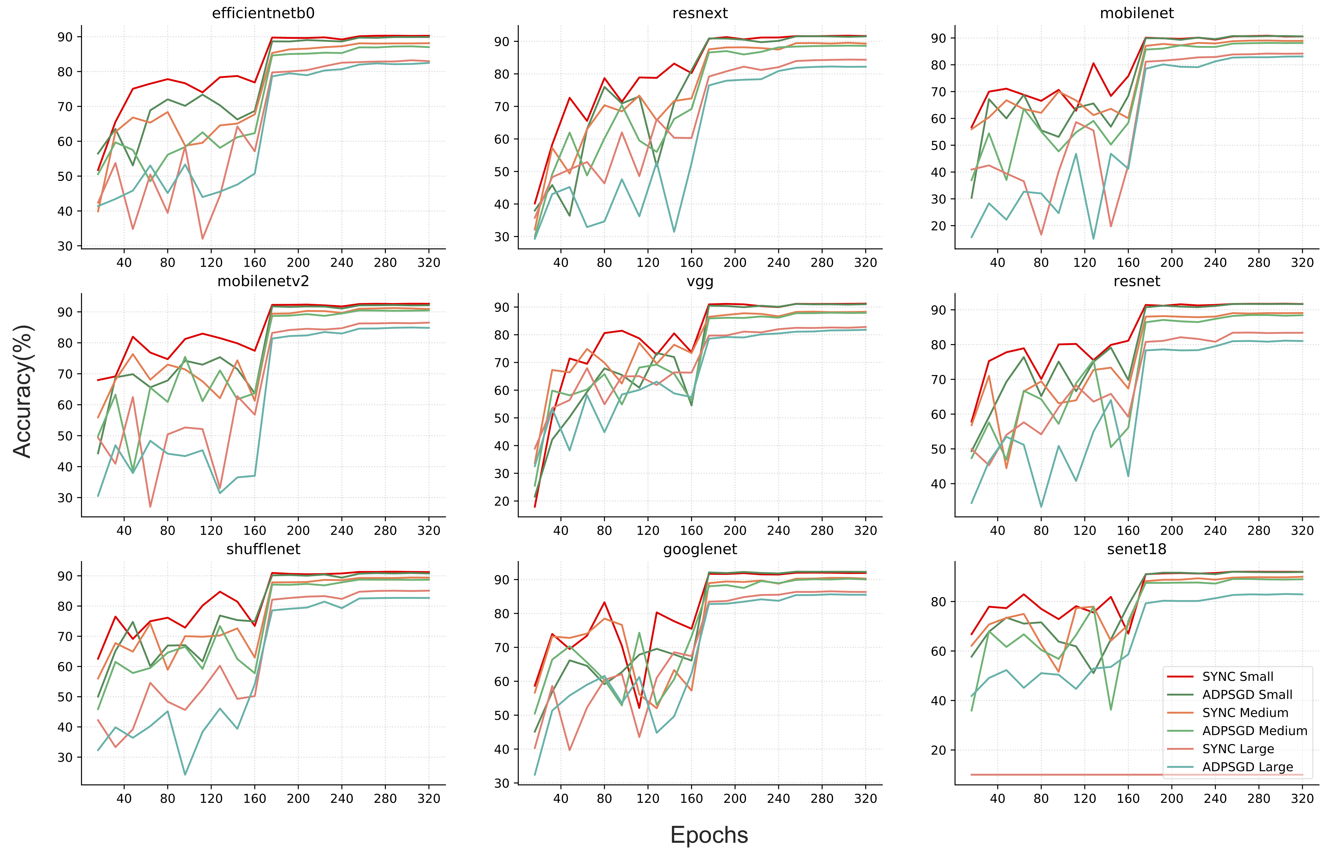
The remaining columns in Table 1 summarize the convergence comparison between SYNC and ADPSGD under various levels of noise. Baseline ADPSGD can outperform SYNC due to ADPSGD’s intrinsic noise can lead model training to a better generalizationinterspeech19 when batchsize is large. Figure 1 visualizes the convergence comparison of three models between SYNC and ADPSGD on CIFAR-10. More results are provided in Appendix B.

Summary ADPSGD and SYNC achieve the comparable level of utility under the same level of noise injection, thus ensuring the same level of differential privacy budget.

5.3 Deployment in the Wild

Federated learning is most often deployed in a heterogeneous environment where different learners are widespread across different type of network links and run on different types of computing devices. We compare SYNC and ADPSGD for various noise levels (i.e. differential privacy budgets) in 3 case studies. More results are provided in Appendix B.

Case I: Random learner slowdown

In this scenario, during iteration there is a random learner that runs 2X slower than normal. This could happen when some learner randomly encounters a system hiccup (e.g., cache misses). In SYNC, every learner must wait for the slowest one thus the whole system slows down by a factor of 2. In contrast, ADPSGD naturally balances the workload and remains largely undisturbed. Figure 2 illustrates the convergence w.r.t runtime comparison between SYNC and ADPSGD on CIFAR-10 when a random learner is slowed down by 2X in each iteration for medium-level noise (for the sake of brevity, we omit the comparison for other levels of noise, as they exhibit similar behaviors).

Figure 1: CIFAR-10 convergence comparison between SYNC and ADPSGD under various levels of noise injection (i.e., differential privacy budget). SYNC and ADPSGD achieve similar level of utilities (i.e. test accuracy).

Case II: One very slow learner

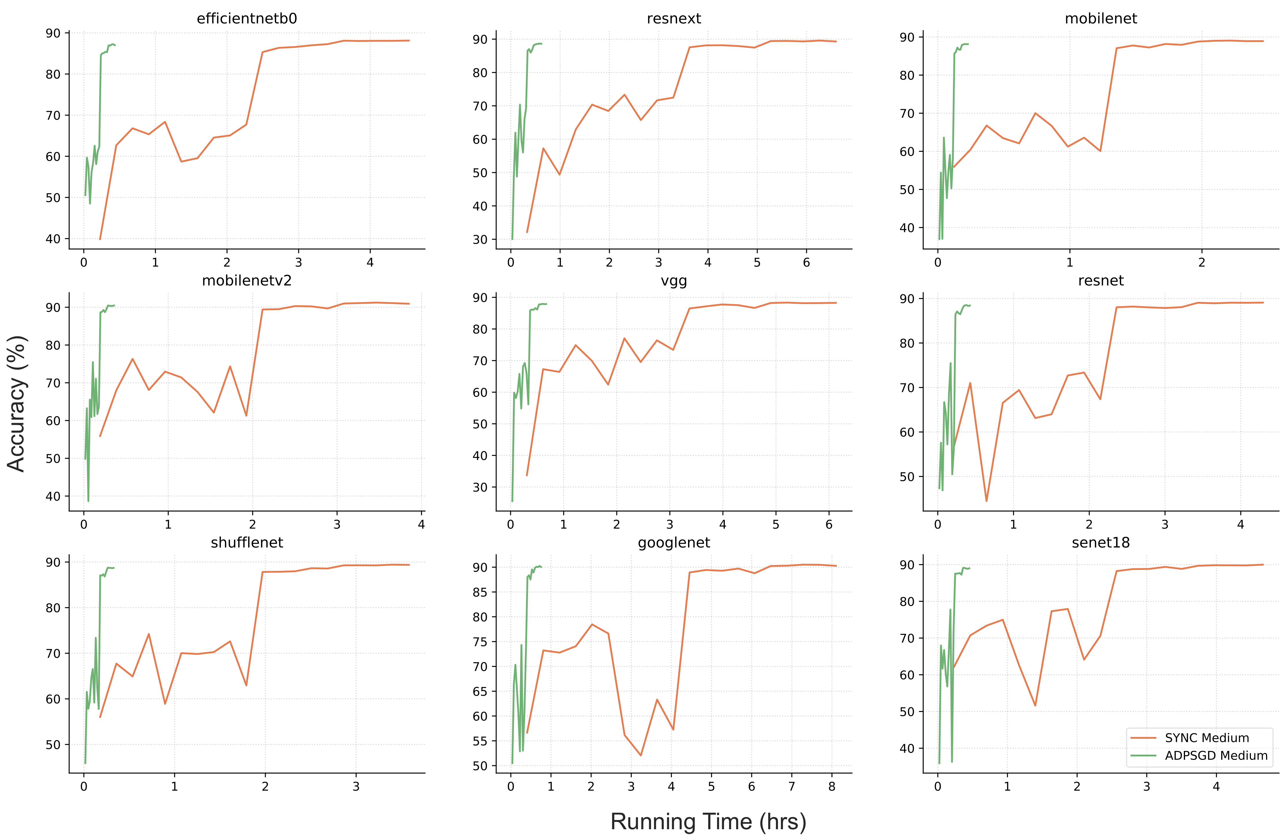
In this scenario, one learner is 10X slower than all the other learners. This could happen when one learner runs on an outdated device or the network links that go into the learners are low-speed compared to others. Similar to Case I, in SYNC, all the learners wait for the slowest one and in ADPSGD, the workload is naturally re-balanced. Figure 3 illustrates the convergence w.r.t runtime comparison of three models between SYNC and ADPSGD on CIFAR-10 when 1 learner is slowed down by 10X in each iteration for medium-level noise.

Case III: Training with Large Batch

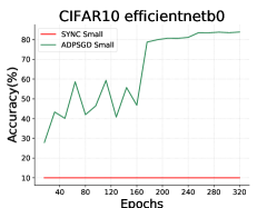
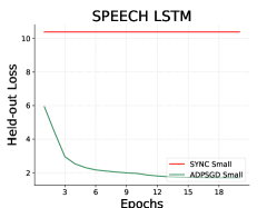
To reduce communication cost, practitioners usually prefer to train with a larger batch size. When training with a larger batch-size, one also needs to scale up the learning rate to ensure a faster convergence interspeech19 ; facebook-1hr ; zhang2015staleness . It was first reported in interspeech19 that SYNC training could collapse for SWB300 task when batch size is large and learning rate is high whereas ADPSGD manages to converge. We found some models (e.g., EfficientNet-B0) for computer vision task also exhibit the same trend. We increase batch size per GPU by a factor of two for CIFAR-10 and SWB300, scale up the corresponding learning rate by 2 and introduce small level of noise, SYNC collapses whereas ADPSGD still converges. Figure 4 shows when batch size is 2X large, SYNC training collapses for CIFAR-10 (EfficientNet-B0 model) and SWB300, but ADPSGD manages to converge for both models.

Figure 2: CIFAR-10 convergence when a random learner is slowed down by 2X in each iteration with medium level of noise injection.

Figure 3: CIFAR-10 convergence when one learner is slowed down by 10X in each iteration with medium level of noise injection. ADPSGD runs significantly faster than SYNC due to its asynchronous nature.

(a) CIFAR-10

(b) SWB300

Figure 4: When batch size is 2X larger and learning rate is 2X larger, ADPSGD converges whereas SYNC does not, with small level of noise injection.

Summary In the heterogeneous environment where federated learning often operates in, ADPSGD achieves much faster convergence than SYNC and ADPSGD can perform well in the case when SYNC does not even converge. Since SYNC often yields the most accurate model among all DDL algorithms, we can safely conclude ADPSGD also achieves the best possible model accuracy in a DP setting, at a much higher speed.

6 Conclusion

This paper presents a differentially private version of asynchronous decentralized parallel SGD, maintaining communication efficiency and preventing inference from malicious participants at the same time. We theoretically analyze the impact of DP mechanism on the convergence of ADPSGD. Our analysis shows A(DP)²SGD also converges at the optimal $\mathcal{O}(1/\sqrt{T})$ rate as SGD. Besides, the privacy and utility guarantees are provided where Rényi differential privacy is introduced to provide tighter privacy analysis for the composite Gaussian mechanism. Finally, we evaluate A(DP)²SGD on both computer vision and speech recognition tasks, and the results demonstrate that it can achieve comparable utility than differentially private version of synchronous SGD but much faster than its synchronous counterparts in heterogeneous computing environments. Future work will focus on adaptive noise level associated with gradient clipping under asynchronous decentralized setting.

Broader Impact Statement

This paper studies the problem of developing differentially private asynchronous decentralized parallel stochastic gradient descent (ADPSGD). Privacy and security are essential problems in real world applications involving sensitive information such as healthcare and criminal justice. The decentralized optimization setting can greatly enhance the security of the model training process and protect the data privacy at different locations. However, the parameter sharing and transmission process can still leak sensitive information. The DP mechanism further protects this potentially vulnerable step and makes the entire process more secure. The proposed A(DP)²SGD mechanism can be broadly applied in the training process of a variety set of machine learning models, and also enhance their trustworthiness in applications involving sensitive information.

Appendix A System Design and Implementation

Most (if not all) of the state-of-the-art DL models are trained in the Synchronous SGD fashion, as it is considered to have the most stable convergence behavior  facebook-1hr ; revisit-sync-sgd ; zhang2016icdm and often yields the best model accuracy. No existing FL training method has been proven to outperform SYNC for the final model accuracy. We implement Synchronous SGD (SYNC) as the "golden" baseline to examine if A(DP)²SGD can achieve the best possbile model accuracy while maintaining DP protection. In SYNC, we place an “allreduce” (sum) call after each learner’s weight update in each iteration and then take the average of the weights across all the learners. An allreduce call is a reduction operation followed by a broadcast operation. A reduction operation is both commutative and associative (e.g., summation). The allreduce mechanism we chose is Nvidia NCCL  nccl , which is the state-of-the-art allreduce implementation on a GPU cluster.

To implement ADPSGD, we place all the learners (i.e., GPUs) on a communication ring. To avoid deadlock, we partition the communication ring into nonintersecting sets of senders and receivers and require that communication edges start from the sender sub-graph and end in the receiver sub-graph. To achieve better convergence behavior, we also adopt the communication randomization technique as proposed in  icassp20 , in which sender randomly picks a receiver in each iteration. The paired-up sender and receiver exchange weights and update their weights as the average of the two. A global counter is maintained to record how many minibatches all the learners in the system collectively have processed. The training finishes when the global counter reaches the termination threshold. We implemented ADPSGD in C++ and MPI.

In both SYNC and ADPSGD, we insert random noise into gradients in each iteration to enable differential privacy protection.

Appendix B Additional Experiment Results

B.1 Software and Hardware

We use PyTorch 1.1.0 as the underlying deep learning framework. We use the CUDA 10.1 compiler, the CUDA-aware OpenMPI 3.1.1, and g++ 4.8.5 compiler to build our communication library, which connects with PyTorch via a Python-C interface. We run our experiments on a 16-GPU 2-server cluster. Each server has 2 sockets and 9 cores per socket. Each core is an Intel Xeon E5-2697 2.3GHz processor. Each server is equipped with 1TB main memory and 8 V100 GPUs. Between servers are 100Gbit/s Ethernet connections. GPUs and CPUs are connected via PCIe Gen3 bus, which has a 16GB/s peak bandwidth in each direction per CPU socket.

B.2 Dataset and Model

We evaluate on two deep learning tasks: computer vision and speech recognition. For computer vision task, we evaluate on CIFAR-10 dataset krizhevsky2009learning , which comprises of a total of 60,000 RGB images of size 32 $\times$ 32 pixels partitioned into the training set (50,000 images) and the test set (10,000 images). We test CIFAR-10 with 9 representative convolutional neural network (CNN) models pytorch-cifar : (1) ShuffleNet, a 50 layer instantiation of ShuffleNet architecture shufflenet . (2) MobileNetV2, a 19 layer instantiation of mobilenetv2 architecture that improves over MobileNet by introducing linear bottlenecks and inverted residual block.(3) EfficientNet-B0, with a compound coefficient 0 in the basic EfficientNet architecture efficientnet . (4) MobileNet, a 28 layer instantiation of MobileNet architecture mobilenet . (5) GoogleNet, a 22 layer instantiation of Inception architecture googlenet . (6) ResNext-29, a 29 layer instantiation of resnext with bottlenecks width 64 and 2 sets of aggregated transformations. (7) ResNet-18, a 18 layer instantiation of ResNet architecture resnet .(8) SENet-18, which stacks Squeeze-and-Excitation blocks senet on top of a ResNet-18 model. (9) VGG-19, a 19 layer instantiation of VGG architecture vgg . The detailed model implementation refers to pytorch-cifar .

Among these models, ShuffleNet, MobileNet(V2), EfficientNet represent the low memory footprint models that are widely used on mobile devices, where federated learnings is often used. The other models are standard CNN models that aim for high accuracy.

For speech recognition task, we evaluate on SWB300 dataset. The training dataset is 30GB large and contains roughly 4.2 million samples. The test dataset is 564MB large and contains roughly 80,000 samples. The acoustic model is a long short-term memory (LSTM) model with 6 bi-directional layers. Each layer contains 1,024 cells (512 cells in each direction). On top of the LSTM layers, there is a linear projection layer with 256 hidden units, followed by a softmax output layer with 32,000 (i.e. 32,000 classes) units corresponding to context-dependent HMM states. The LSTM is unrolled with 21 frames and trained with non-overlapping feature subsequences of that length. The feature input is a fusion of FMLLR (40-dim), i-Vector (100-dim), and logmel with its delta and double delta (40-dim $\times$3). This model contains over 43 million parameters and is about 165MB large.

Table 2 summarizes the model size and training time for both tasks. Training time is measured on running single-GPU and accounts the time for collecting training statistics (e.g., L2-Norm) and noise injection operations.

Model/Dataset	Model Size (MB)	Training Time (hr)
ShuffleNet/C*	4.82	4.16
MobileNetV2/C	8.76	4.63
EfficientNet-B0/C	11.11	5.53
MobileNet/C	12.27	3.55
GoogleNet/C	23.53	8.43
ResNext-29/C	34.82	7.08
ResNet-18/C	42.63	5.56
SENet-18/C	42.95	5.80
VGG-19/C	76.45	7.42
LSTM/S**	164.62	102.41

Table 2: Model size and training time. Training time is measured on running on 1 V100 GPU, which accounts additional operations for collecting training statistics (e.g., L2-Norm) and noise injection operations. *C stands for CIFAR-10, **S stands for SWB300.

Figure 5: CIFAR-10 convergence comparison between SYNC and ADPSGD under various levels of noise injection (i.e., differential privacy budget). SYNC and ADPSGD achieve similar level of utilities (i.e. test accuracy).

Figure 6: CIFAR-10 convergence when one learner is slowed down by 10X in each iteration with medium level of noise injection. ADPSGD runs significantly faster than SYNC due to its asynchronous nature.

Figure 7: CIFAR-10 convergence when one learner is slowed down by 10X in each iteration with medium level of noise injection (we omit displaying other levels of noise for the sake of brevity). ADPSGD runs significantly faster than SYNC due to its asynchronous nature.

Figure 7 depicts the convergence comparison between SYNC and ADPSGD on CIFAR-10 when 1 learner is slowed down by 10X.

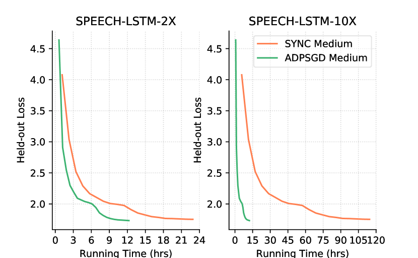
Figure 9 depicts the convergence comparison between SYNC and ADPSGD on SWB300 task for Case I and case II.

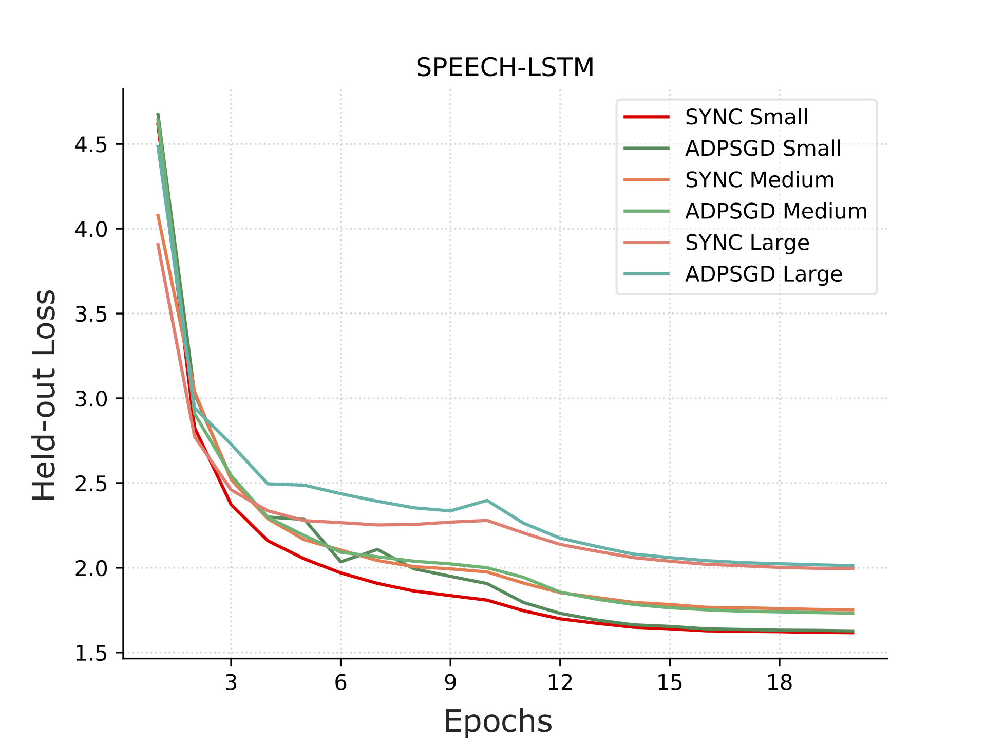
Figure 8: SWB300 convergence comparison between SYNC and ADPSGD under various levels of noise injection (i.e., differential privacy budget). SYNC and ADPSGD achieve similar level of utilities (i.e. held-out loss).

Figure 9: SWB300 convergence when one random learner is slowed down by 2X (left) and one learner is slowed down by 10X (right), with medium level noise injection (we omit displaying other levels of noise for the sake of brevity). ADPSGD runs significantly faster than SYNC due to its asynchronous nature.

Appendix C Proofs of Theorem 1

Proof.

Recall that we have the following update rule:

$$[\mathbf{w}_{1}^{t+1/2},\mathbf{w}_{2}^{t+1/2},...,\mathbf{w}_{K}^{t+1/2}]\leftarrow[\mathbf{w}_{1}^{t},\mathbf{w}_{2}^{t},...,\mathbf{w}_{K}^{t}]\mathbf{A}^{t};$$

$$\mathbf{w}_{k^{t}}^{t+1}\leftarrow\mathbf{w}_{k^{t}}^{t+1/2}-\eta\left({g}^{t}(\hat{\mathbf{w}}_{k^{t}}^{t};\xi_{k^{t}}^{t})+\mathbf{n}\right),$$ (9)

where $k^{t}$ are drawn from $[K]$, and $\mathbf{n}\sim\mathcal{N}(0,\sigma^{2}\mathbf{I})$. Let’s denote $\theta^{t+1}$ as the average of all local models at $\{t+1\}$-th iteration, i.e., $\theta^{t+1}=\frac{1}{K}\sum_{k=1}^{K}\mathbf{w}_{k}^{t+1}$. Since $F$ is $L$-smooth, we have

$$F(\theta^{t+1})= F\left(\frac{\mathbf{W}^{t+1}\mathbf{1}_{K}}{K}\right)=F\left(\frac{\mathbf{W}^{t}\mathbf{A}^{t}\mathbf{1}_{K}}{K}-\frac{\eta}{K}\left(g_{c}(\hat{\mathbf{w}}_{k^{t}}^{t},\xi_{k^{t}}^{t})+\mathbf{n}\right)\right)$$

$$= F\left(\frac{\mathbf{W}^{t}\mathbf{1}_{K}}{K}-\frac{\eta}{K}\left(g_{c}(\hat{\mathbf{w}}_{k^{t}}^{t},\xi_{k^{t}}^{t})+\mathbf{n}\right)\right)=F\left(\theta^{t}-\frac{\eta}{K}\left(g_{c}(\hat{\mathbf{w}}_{k^{t}}^{t},\xi_{k^{t}}^{t})+\mathbf{n}\right)\right)$$

$$\leq F\left(\theta^{t}\right)-\frac{\eta}{K}\left\langle\triangledown F(\theta^{t}),\left(g_{c}(\hat{\mathbf{w}}_{k^{t}}^{t},\xi_{k^{t}}^{t})+\mathbf{n}\right)\right\rangle$$

$$\ \ \ +\frac{\eta^{2}L}{2K^{2}}\left(\left\|g_{c}(\hat{\mathbf{w}}_{k^{t}}^{t},\xi_{k^{t}}^{t})\right\|^{2}+\|\mathbf{n}\|^{2}+2\left\langle g_{c}(\hat{\mathbf{w}}_{k^{t}}^{t},\xi_{k^{t}}^{t}),\mathbf{n}\right\rangle\right).$$

Tanking expectation with respect to $k^{t}$ and $\mathbf{n}$ given $\theta^{t}$, we have

$$\mathbb{E}F(\theta^{t+1})-\mathbb{E}F(\theta^{t})$$

$$\leq -\frac{\eta}{K}\mathbb{E}\left\langle\triangledown F(\theta^{t}),g(\hat{\mathbf{w}}_{k^{t}}^{t},\xi_{k^{t}}^{t})\right\rangle+\frac{\eta^{2}L}{2K^{2}}\left(\mathbb{E}\left\|g(\hat{\mathbf{w}}_{k^{t}}^{t},\xi_{k^{t}}^{t})\right\|^{2}+\mathbb{E}\|\mathbf{n}\|^{2}\right)$$

$$\leq -\frac{\eta B}{K}\mathbb{E}\left\langle\triangledown F(\theta^{t}),\sum_{k=1}^{K}p_{k}\triangledown F_{k}(\hat{\mathbf{w}}_{k}^{t})\right\rangle+\frac{\eta^{2}L}{2K^{2}}\mathbb{E}\|g(\hat{\mathbf{w}}_{k^{t}}^{t};\xi_{k^{t}}^{t})\|^{2}+\frac{\eta^{2}Ld\sigma^{2}}{2K^{2}}$$

$$= \frac{\eta B}{2K}\underbrace{\mathbb{E}\left\|\triangledown F(\theta^{t})-\sum_{k=1}^{K}p_{k}\triangledown F_{k}(\hat{\mathbf{w}}_{k}^{t})\right\|^{2}}_{T_{1}}-\frac{\eta B}{2K}\mathbb{E}\left\|\sum_{k=1}^{K}p_{k}\triangledown F_{k}(\hat{\mathbf{w}}_{k}^{t})\right\|^{2}$$

$$-\frac{\eta B}{2K}\mathbb{E}\left\|\triangledown F(\theta^{t})\right\|^{2}+\frac{\eta^{2}L}{2K^{2}}\underbrace{\mathbb{E}\left\|g(\hat{\mathbf{w}}_{k^{t}}^{t},\xi_{k^{t}}^{t})\right\|^{2}}_{T_{2}}+\frac{\eta^{2}Ld\sigma^{2}}{2K^{2}}.$$ (10)

For $T_{1}$ we have

$$T_{1}= \mathbb{E}\left\|\triangledown F(\theta^{t})-\sum_{k=1}^{K}p_{k}\triangledown F_{k}(\hat{\mathbf{w}}_{k}^{t})\right\|^{2}$$

$$\leq 2\mathbb{E}\left\|\triangledown F(\theta^{t})-\triangledown F(\hat{\theta}^{t})\right\|^{2}+2\mathbb{E}\left\|\triangledown F(\hat{\theta}^{t})-\sum_{k=1}^{K}p_{k}\triangledown F_{k}(\hat{\mathbf{w}}_{k}^{t})\right\|^{2}$$

$$= 2\mathbb{E}\left\|\triangledown F(\theta^{t})-\triangledown F(\hat{\theta}^{t})\right\|^{2}+2\mathbb{E}\left\|\sum_{k=1}^{K}p_{k}\left(\triangledown F_{k}(\hat{\theta}^{t})-\triangledown F_{k}(\hat{\mathbf{w}}_{k}^{t})\right)\right\|^{2}$$

$$\leq 2\mathbb{E}\left\|\triangledown F(\theta^{t})-\triangledown F(\hat{\theta}^{t})\right\|^{2}+2\mathbb{E}\sum_{k=1}^{K}p_{k}\left\|\triangledown F_{k}(\hat{\theta}^{t})-\triangledown F_{k}(\hat{\mathbf{w}}_{k}^{t})\right\|^{2}$$

$$\leq 2L^{2}\mathbb{E}\left\|\theta^{t}-\hat{\theta}^{t}\right\|^{2}+2L^{2}\mathbb{E}\sum_{k=1}^{K}p_{k}\left\|\hat{\theta}^{t}-\hat{\mathbf{w}}_{k}^{t}\right\|^{2}$$

$$= 2L^{2}\mathbb{E}\left\|\sum_{t^{\prime}=1}^{\tau_{t}}\frac{\eta}{K}g(\hat{\mathbf{w}}_{k^{t-t^{\prime}}}^{t-t^{\prime}},\xi_{k^{t-t^{\prime}}}^{t-t^{\prime}})\right\|^{2}+2L^{2}\mathbb{E}\sum_{k=1}^{K}p_{k}\left\|\hat{\theta}^{t}-\hat{\mathbf{w}}_{k}^{t}\right\|^{2}$$

$$\leq \frac{2\eta^{2}L^{2}\tau_{t}}{K^{2}}\sum_{t^{\prime}=1}^{\tau_{t}}\mathbb{E}\left\|g(\hat{\mathbf{w}}_{k^{t-t^{\prime}}}^{t-t^{\prime}},\xi_{k^{t-t^{\prime}}}^{t-t^{\prime}})\right\|^{2}+2L^{2}\mathbb{E}\sum_{k=1}^{K}p_{k}\left\|\hat{\theta}^{t}-\hat{\mathbf{w}}_{k}^{t}\right\|^{2}.$$ (11)

For $T_{2}$, we have

$$T_{2}= \mathbb{E}\left\|g(\hat{\mathbf{w}}_{k^{t}}^{t},\xi_{k^{t}}^{t})\right\|^{2}=\sum_{k=1}^{K}p_{k}\mathbb{E}\left\|\sum_{j=1}^{B}\triangledown f_{j}(\hat{\mathbf{w}}_{k}^{t},\xi_{k}^{t,j})\right\|^{2}$$

$$= \sum_{k=1}^{K}p_{k}\mathbb{E}\left\|\sum_{j=1}^{B}\left(\triangledown f(\hat{\mathbf{w}}_{k}^{t},\xi_{k}^{t,j})-\triangledown F_{k}(\hat{\mathbf{w}}_{k}^{t})\right)\right\|^{2}+\sum_{k=1}^{K}p_{k}\mathbb{E}\left\|B\triangledown F_{k}(\hat{\mathbf{w}}_{k}^{t})\right\|^{2}$$

$$\leq B\varsigma^{2}+B^{2}\sum_{k=1}^{K}p_{k}\mathbb{E}\left\|\triangledown F_{k}(\hat{\mathbf{w}}_{k}^{t})\right\|^{2}.$$ (12)

According to Lemma 5 in lian2018asynchronous , we have

$$\sum_{k=1}^{K}p_{k}\mathbb{E}\left\|\triangledown F_{k}(\hat{\mathbf{w}}_{k}^{t})\right\|^{2}\leq 12L^{2}\mathbb{E}\sum_{k=1}^{K}p_{k}^{2}\left\|\hat{\theta}^{t}-\hat{\mathbf{w}}_{k}^{t}\right\|^{2}+6\upsilon^{2}+2\mathbb{E}\left\|\sum_{k=1}^{K}p_{k}\triangledown F_{k}(\hat{\mathbf{w}}_{k}^{t})\right\|^{2}.$$

Plugging (C), (C) and (C) into (C), we can obtain

$$\mathbb{E}F(\theta^{t+1})-\mathbb{E}F(\theta^{t})$$

$$\stackrel{{\scriptstyle(\ref{eq:T1})}}{{\leq}} \frac{\eta B}{K}\left(\frac{\eta^{2}L^{2}\tau_{t}}{K^{2}}\sum_{t^{\prime}=1}^{\tau_{t}}\mathbb{E}\left\|g(\hat{\mathbf{w}}_{k^{t-t^{\prime}}}^{t-t^{\prime}},\xi_{k^{t-t^{\prime}}}^{t-t^{\prime}})\right\|^{2}+L^{2}\mathbb{E}\sum_{k=1}^{K}p_{k}\left\|\hat{\theta}^{t}-\hat{\mathbf{w}}_{k}^{t}\right\|^{2}\right)$$

$$-\frac{\eta B}{2K}\mathbb{E}\left\|\sum_{k=1}^{K}p_{k}\triangledown F_{k}(\hat{\mathbf{w}}_{k}^{t})\right\|^{2}-\frac{\eta B}{2K}\mathbb{E}\left\|\triangledown F(\theta^{t})\right\|^{2}$$

$$+\frac{\eta^{2}L}{2K^{2}}\mathbb{E}\left\|g(\hat{\mathbf{w}}_{k^{t}}^{t},\xi_{k^{t}}^{t})\right\|^{2}+\frac{\eta^{2}Ld\sigma^{2}}{2K^{2}}$$

$$\stackrel{{\scriptstyle(\ref{eq:T2})}}{{\leq}} \frac{\eta^{3}L^{2}B^{3}\tau_{t}}{K^{3}}\sum_{t^{\prime}=1}^{\tau_{t}}\sum_{k=1}^{K}p_{k}\mathbb{E}\left\|\triangledown F_{k}(\hat{\mathbf{w}}_{k}^{t-t^{\prime}})\right\|^{2}+\frac{\eta L^{2}B}{K}\mathbb{E}\sum_{k=1}^{K}p_{k}\left\|\hat{\theta}^{t}-\hat{\mathbf{w}}_{k}^{t}\right\|^{2}$$

$$-\frac{\eta B}{2K}\mathbb{E}\left\|\sum_{k=1}^{K}p_{k}\triangledown F_{k}(\hat{\mathbf{w}}_{k}^{t})\right\|^{2}-\frac{\eta B}{2K}\mathbb{E}\left\|\triangledown F(\theta^{t})\right\|^{2}+\frac{\eta^{2}LB^{2}}{2K^{2}}\sum_{k=1}^{K}p_{k}\mathbb{E}\left\|\triangledown F_{k}(\hat{\mathbf{w}}_{k}^{t})\right\|^{2}$$

$$+\frac{\eta^{2}L(\varsigma^{2}B+d\sigma^{2})}{2K^{2}}+\frac{\eta^{3}L^{2}B^{2}\varsigma^{2}\tau_{t}^{2}}{K^{3}}$$

$$\stackrel{{\scriptstyle(\ref{eq:lem5})}}{{\leq}} \frac{2\eta^{3}L^{2}B^{3}\tau}{K^{3}}\sum_{t^{\prime}=1}^{\tau_{t}}\left(6L^{2}\mathbb{E}\sum_{k=1}^{K}p_{k}\left\|\hat{\theta}^{t-t^{\prime}}-\hat{\mathbf{w}}_{k}^{t-t^{\prime}}\right\|^{2}+\mathbb{E}\left\|\sum_{k=1}^{K}p_{k}\triangledown F_{k}(\hat{\mathbf{w}}_{k}^{t-t^{\prime}})\right\|^{2}\right)$$

$$-\frac{\eta B}{2K}\mathbb{E}\left\|\triangledown F(\theta^{t})\right\|^{2}+\left(\frac{\eta L^{2}B}{K}+\frac{6\eta^{2}L^{3}B^{2}}{K^{2}}\right)\mathbb{E}\sum_{k=1}^{K}p_{k}\left\|\hat{\theta}^{t}-\hat{\mathbf{w}}_{k}^{t}\right\|^{2}$$

$$-\left(\frac{\eta B}{2K}-\frac{\eta^{2}LB^{2}}{K^{2}}\right)\mathbb{E}\left\|\sum_{k=1}^{K}p_{k}\triangledown F_{k}(\hat{\mathbf{w}}_{k}^{t})\right\|^{2}$$

$$+\frac{\eta^{2}L(\varsigma^{2}B+6\upsilon^{2}B^{2}+d\sigma^{2})}{2K^{2}}+\frac{\eta^{3}L^{2}B^{2}\tau^{2}(\varsigma^{2}+6\upsilon^{2}B)}{K^{3}}.$$

Summing over $t=0,...,T-1$ and $\forall\tau_{t}\leq\tau$, we have

$$\mathbb{E}F(\theta^{t+1})-\mathbb{E}F(\theta^{t})$$

$$\leq \frac{2\eta^{3}B^{3}L^{2}\tau^{2}}{K^{3}}\sum_{t=0}^{T-1}\left(6L^{2}\mathbb{E}\sum_{k=1}^{K}p_{k}\left\|\hat{\theta}^{t}-\hat{\mathbf{w}}_{k}^{t}\right\|^{2}+\mathbb{E}\left\|\sum_{k=1}^{K}p_{k}\triangledown F_{k}(\hat{\mathbf{w}}_{k}^{t})\right\|^{2}\right)$$

$$-\left(\frac{\eta B}{2K}-\frac{\eta^{2}B^{2}L}{K^{2}}\right)\sum_{t=0}^{T-1}\mathbb{E}\left\|\sum_{k=1}^{K}p_{k}\triangledown F_{k}(\hat{\mathbf{w}}_{k}^{t})\right\|^{2}-\frac{\eta B}{2K}\sum_{t=0}^{T-1}\mathbb{E}\left\|\triangledown F(\theta^{t})\right\|^{2}$$

$$+\left(\frac{\eta BL^{2}}{K}+\frac{6\eta^{2}B^{2}L^{3}}{K^{2}}\right)\sum_{t=0}^{T-1}\mathbb{E}\sum_{k=1}^{K}p_{k}\left\|\hat{\theta}^{t}-\hat{\mathbf{w}}_{k}^{t}\right\|^{2}$$

$$+\frac{\eta^{3}BL^{2}\tau^{2}(\varsigma^{2}B+6\upsilon^{2}B^{2}+d\sigma^{2})T}{K^{3}}+\frac{\eta^{2}L(\varsigma^{2}B+6\upsilon^{2}B^{2}+d\sigma^{2})T}{2K^{2}}$$

$$= \left(\frac{\eta BL^{2}}{K}+\frac{6\eta^{2}B^{2}L^{3}}{K^{2}}+\frac{12\eta^{3}B^{3}L^{4}\tau^{2}}{K^{3}}\right)\underbrace{\sum_{t=0}^{T-1}\mathbb{E}\sum_{k=1}^{K}p_{k}\left\|\hat{\theta}^{t}-\hat{\mathbf{w}}_{k}^{t}\right\|^{2}}_{T_{3}}$$

$$-\left(\frac{\eta B}{2K}-\frac{\eta^{2}B^{2}L}{K^{2}}-\frac{2\eta^{3}B^{3}L^{2}\tau^{2}}{K^{3}}\right)\sum_{t=0}^{T-1}\mathbb{E}\left\|\sum_{k=1}^{K}p_{k}\triangledown F_{k}(\hat{\mathbf{w}}_{k}^{t})\right\|^{2}-\frac{\eta B}{2K}\sum_{t=0}^{T-1}\mathbb{E}\left\|\triangledown F(\theta^{t})\right\|^{2}$$

$$+\frac{\eta^{3}BL^{2}\tau^{2}(\varsigma^{2}B+6\upsilon^{2}B^{2}+d\sigma^{2})T}{K^{3}}+\frac{\eta^{2}L(\varsigma^{2}B+6\upsilon^{2}B^{2}+d\sigma^{2})T}{2K^{2}}$$ (13)

We can use Lemma 1 to bound the term $T_{3}$ and we use similar notations as in lian2018asynchronous for simpler notation. By arranging the terms, we have

$$\mathbb{E}F(\theta^{T})\leq \mathbb{E}F(\theta^{0})-C_{2}\sum_{t=0}^{T-1}\mathbb{E}\left\|\sum_{k=1}^{K}p_{k}\triangledown F_{k}(\hat{\mathbf{w}}_{k}^{t})\right\|^{2}-\frac{\eta B}{2K}\sum_{t=0}^{T-1}\mathbb{E}\left\|\triangledown F(\theta^{t})\right\|^{2}$$

$$+C_{3}\frac{\eta^{2}LT}{K^{2}}(\varsigma^{2}B+6\upsilon^{2}B^{2}+d\sigma^{2}).$$ (14)

Then, while $C_{3}\leq 1$ and $C_{2}\geq 0$ we complete the proof of Theorem 1.

$$\frac{\sum_{t=0}^{T-1}\mathbb{E}\left\|\triangledown F(\theta^{t})\right\|^{2}}{T}\leq \frac{2\left(\mathbb{E}F(\theta^{0})-\mathbb{E}F(\theta^{T})\right)}{\eta TB/K}+\frac{2\eta L}{BK}(\varsigma^{2}B+6\upsilon^{2}B^{2}+d\sigma^{2})$$

$$\leq \frac{2\left(\mathbb{E}F(\mathbf{w}^{0})-\mathbb{E}F^{*}\right)}{\eta TB/K}+\frac{2\eta L}{BK}(\varsigma^{2}B+6\upsilon^{2}B^{2}+d\sigma^{2}).$$

We complete the proof. ∎

Appendix D Proofs of Lemma 1

Lemma 1.

While $C_{1}>0$ and $\forall T\geq 1$, we have

$$\frac{\sum_{t=0}^{T-1}\mathbb{E}\sum_{k=1}^{K}p_{k}\left\|\hat{\theta}^{t}-\hat{\mathbf{w}}_{k}^{t}\right\|^{2}}{T}\leq \frac{4\eta^{2}B^{2}}{TC_{1}}\left(\tau\frac{K-1}{K}+\bar{\rho}\right)\sum_{t=0}^{T-1}\mathbb{E}\left\|\sum_{k=1}^{K}p_{k}\triangledown F_{k}(\hat{\mathbf{w}}_{k}^{t})\right\|^{2}$$

$$\quad\quad\quad+\frac{2\eta^{2}(\varsigma^{2}B+6\upsilon^{2}B^{2}+d\sigma^{2})\bar{\rho}}{C_{1}}$$ (15)

Proof.

First, we have

$$\mathbb{E}\left\|g(\hat{\mathbf{w}}_{k^{t}}^{t},\xi_{k^{t}}^{t})+\mathbf{n}-B\triangledown F_{k^{t}}(\mathbf{w}_{k^{t}}^{t})\right\|^{2}$$

$$= \mathbb{E}\left\|g(\hat{\mathbf{w}}_{k^{t}}^{t},\xi_{k^{t}}^{t})-B\triangledown F_{k^{t}}(\mathbf{w}_{k^{t}}^{t})\right\|^{2}+\mathbb{E}\|\mathbf{n}\|^{2}\leq B\varsigma^{2}+d\sigma^{2}.$$ (16)

According to our updating rule and Lemma 6 in lian2018asynchronous , we can obtain

$$\mathbb{E}\left\|\theta^{t+1}-\mathbf{w}_{k}^{t+1}\right\|^{2}$$

$$= \mathbb{E}\left\|\theta^{t}-\frac{\eta}{K}(g(\hat{\mathbf{w}}_{k^{t}}^{t},\xi_{k^{t}}^{t})+\mathbf{n})-\left(\mathbf{W}^{t}\mathbf{A}^{t}\mathbf{e}_{k}-\eta\tilde{g}(\hat{\mathbf{W}}^{t},\xi_{k^{t}}^{t})\mathbf{e}_{k}\right)\right\|^{2}$$

$$\leq 2\eta^{2}B^{2}\frac{K-1}{K}\mathbb{E}\sum_{j=0}^{t}\left(12L^{2}\sum_{k=1}^{K}p_{k}\left\|\hat{\theta}^{j}-\hat{\mathbf{w}}_{k}^{j}\right\|^{2}+2\mathbb{E}\left\|\sum_{k=1}^{K}p_{k}\triangledown F_{k}(\hat{\mathbf{w}}_{k}^{j})\right\|^{2}\right)$$

$$\times(\rho^{t-j}+2(t-j)\rho^{\frac{t-j}{2}})+2\eta^{2}(\varsigma^{2}B+6\upsilon^{2}B^{2}+d\sigma^{2})\bar{\rho}.$$ (17)

where $\bar{\rho}=\frac{K-1}{K}\left(\frac{1}{1-\rho}+\frac{2\sqrt{\rho}}{(1-\sqrt{\rho})^{2}}\right)$.

Noting that $\hat{\mathbf{W}}^{t}=\mathbf{W}^{t-\tau_{t}}$, then we have

$$\mathbb{E}\sum_{k=1}^{K}p_{k}\left\|\hat{\theta}^{t}-\hat{\mathbf{w}}_{k}^{t}\right\|^{2}=\sum_{k=1}^{K}p_{k}\mathbb{E}\left\|\hat{\theta}^{t}-\hat{\mathbf{w}}_{k}^{t}\right\|^{2}$$

$$\leq 2\eta^{2}B^{2}\frac{K-1}{K}\mathbb{E}\sum_{j=0}^{t-\tau_{t}-1}\left(12L^{2}\sum_{k=1}^{K}p_{k}\left\|\hat{\theta}^{j}-\hat{\mathbf{w}}_{k}^{j}\right\|^{2}+2\mathbb{E}\left\|\sum_{k=1}^{K}p_{k}\triangledown F_{k}(\hat{\mathbf{w}}_{k}^{j})\right\|^{2}\right)$$

$$\times(\rho^{t-\tau_{t}-1-j}+2(t-\tau_{t}-1-j)\rho^{\frac{t-\tau_{t}-1-j}{2}})+2\eta^{2}(\varsigma^{2}B+6\upsilon^{2}B^{2}+d\sigma^{2})\bar{\rho}.$$

According to Lemma 7 in lian2018asynchronous , we can obtain

$$\frac{\sum_{t=0}^{T-1}\sum_{k=1}^{K}p_{k}\mathbb{E}\left\|\hat{\theta}^{t}-\hat{\mathbf{w}}_{k}^{t}\right\|^{2}}{T}$$

$$\leq \frac{2\eta^{2}B^{2}}{T}\frac{K-1}{K}\sum_{t=0}^{T-1}\sum_{j=0}^{t-\tau_{t}-1}\left(12L^{2}\sum_{k=1}^{K}p_{k}\left\|\hat{\theta}^{j}-\hat{\mathbf{w}}_{k}^{j}\right\|^{2}+2\mathbb{E}\left\|\sum_{k=1}^{K}p_{k}\triangledown F_{k}(\hat{\mathbf{w}}_{k}^{j})\right\|^{2}\right)$$

$$\times(\rho^{t-\tau_{t}-1-j}+2(t-\tau_{t}-1-j)\rho^{\frac{t-\tau_{t}-1-j}{2}})+2\eta^{2}(\varsigma^{2}B+6\upsilon^{2}B^{2}+d\sigma^{2})\bar{\rho}$$

$$\leq \frac{4\eta^{2}B^{2}}{T}\left(\tau\frac{K-1}{K}+\bar{\rho}\right)\sum_{t=0}^{T-1}\left(\mathbb{E}\left\|\sum_{k=1}^{K}p_{k}\triangledown F_{k}(\hat{\mathbf{w}}_{k}^{t})\right\|^{2}\right)$$

$$+\frac{24\eta^{2}B^{2}L^{2}}{T}\left(\tau\frac{K-1}{K}+\bar{\rho}\right)\sum_{t=0}^{T-1}\mathbb{E}\sum_{k=1}^{K}p_{k}\left\|\hat{\theta}^{t}-\hat{\mathbf{w}}_{k}^{t}\right\|^{2}+2\eta^{2}(\varsigma^{2}B+6\upsilon^{2}B^{2}+d\sigma^{2})\bar{\rho}.$$ (18)

By rearranging the terms we obtain

$$\underbrace{\left(1-24\eta^{2}B^{2}L^{2}\left(\tau\frac{K-1}{K}+\bar{\rho}\right)\right)}_{C_{1}}\frac{\sum_{t=0}^{T-1}\mathbb{E}\sum_{k=1}^{K}p_{k}\left\|\hat{\theta}^{t}-\hat{\mathbf{w}}_{k}^{t}\right\|^{2}}{T}$$

$$\leq \frac{4\eta^{2}B^{2}}{T}\left(\tau\frac{K-1}{K}+\bar{\rho}\right)\sum_{t=0}^{T-1}\mathbb{E}\left\|\sum_{k=1}^{K}p_{k}\triangledown F_{k}(\hat{\mathbf{w}}_{k}^{t})\right\|^{2}+2\eta^{2}(\varsigma^{2}B+6\upsilon^{2}B^{2}+d\sigma^{2})\bar{\rho}.$$ (19)

We complete the proof. ∎

Appendix E Proofs of Theorem 2

Definition 2 ($(\alpha,\epsilon)$-RDP mironov2017renyi ).

A randomized mechanism $\mathcal{M}:\mathcal{X}^{n}\to\mathcal{R}$ satisfies $\epsilon$-Rényi differential privacy of order $\alpha\in(1,\infty)$, or $(\alpha,\epsilon)$-RDP for short, if for all $\mathbf{x},\mathbf{x}^{\prime}\in\mathcal{X}^{n}$ differing on a single entry, it holds that

$$D_{\alpha}(\mathcal{M}(\mathbf{x})\|\mathcal{M}(\mathbf{x}^{\prime}))\triangleq\frac{1}{\alpha-1}\log\mathbb{E}_{x\sim\mathcal{M}(\mathbf{x}^{\prime})}\left(\frac{\mathcal{M}(\mathbf{x})(x)}{\mathcal{M}(\mathbf{x}^{\prime})(x)}\right)^{\alpha}\leq\epsilon.$$ (20)

The new definition $(\alpha,\epsilon)$-RDP shares many important properties with the standard definition of differential privacy, while additionally allowing for a more rigorous analysis of composite heterogeneous mechanisms mironov2017renyi .

To achieve differential privacy, a stochastic component (typically by additional noise) is usually added to or removed from the locally trained model. Typically, Gaussian mechanism, one of the common choices, injects additive Gaussian noise to the query:

$$\mathcal{M}\triangleq f(\mathbf{x})+\mathcal{N}(0,\sigma^{2}\triangle_{2}^{2}(f)),$$ (21)

where $\mathcal{N}(0,\sigma^{2}\triangle_{2}^{2}(f))$ is the Gaussian distribution noise with mean $0$ and standard deviation $\sigma\triangle_{2}(f)$ which depends on the privacy budget $\epsilon$ as well as the sensitivity of $f$. And the (global) sensitivity of a function $f$ is defined as:

Definition 3 ($l_{p}$-Sensitivity).

The $l_{p}$-sensitivity of a function $f$ is defined by

$$\triangle_{p}(f)=\max_{\mathbf{x},\mathbf{x}^{\prime}}\|f(\mathbf{x})-f(\mathbf{x}^{\prime})\|_{p},$$ (22)

where $\mathbf{x}$ and $\mathbf{x}^{\prime}$ differ in only one entry.

In order to prove Theorem 2, we need the following Lemmas.

Lemma 2 (Gaussian Mechanism  mironov2017renyi ; wang2018subsampled ; wang2019efficient ).

Given a function $f:\mathcal{X}^{n}\rightarrow\mathcal{R}$, the Gaussian Mechanism $\mathcal{M}\triangleq f(\mathbf{x})+\mathcal{N}(0,\sigma^{2}\mathbf{I})$ satisfies $(\alpha,\alpha\triangle_{2}^{2}(f)/(2\sigma^{2}))$-RDP. In addition, if $\mathcal{M}$ is applied to a subset of samples using uniform sampling without replacement $\mathcal{S}_{\gamma}^{\textsf{wo}}$, then $\mathcal{M}^{\mathcal{S}_{\gamma}^{\textsf{wo}}}$ that applies $\mathcal{M}\circ\mathcal{S}_{\gamma}^{\textsf{wo}}$ obeys $(\alpha,5\gamma^{2}\alpha\triangle_{2}^{2}(f)/\sigma^{2})$-RDP when $\sigma^{2}/\triangle_{2}^{2}(f)\geq 1.5$ and $\alpha\leq\log(1/(\gamma(1+\sigma^{2}/\triangle_{2}^{2}(f))))$ with $\gamma$ denoting the subsample rate.

Lemma 3 (Composition  mironov2017renyi ; wang2019efficient ).

Let $\mathcal{M}_{i}:\mathcal{X}^{n}\rightarrow\mathcal{R}_{i}$ be an $(\alpha,\epsilon_{i})$-RDP mechanism for $i\in[k]$. If $\mathcal{M}_{[k]}:\mathcal{X}^{n}\rightarrow\prod_{i=1}^{k}\mathcal{R}_{i}$ is defined to be $\mathcal{M}_{[k]}(\mathbf{x})=(\mathcal{M}_{1}(\mathbf{x}),...,\mathcal{M}_{k}(\mathbf{x}))$, then $\mathcal{M}_{[k]}$ is $(\alpha,\sum_{i=1}^{k}\epsilon_{i})$-RDP. In addition, the input of $\mathcal{M}_{i}$ can be based on the outputs of previous $(i-1)$ mechanisms.

Lemma 4 (From RDP to $(\epsilon,\delta)$-DP  mironov2017renyi ).

If a randomized mechanism $\mathcal{M}:\mathcal{X}^{n}\rightarrow\mathcal{R}$ is $(\alpha,\epsilon)$-RDP, then $\mathcal{M}$ is $(\epsilon+\log(1/\delta)/(\alpha-1),\delta)$-DP, $\forall\delta\in(0,1)$.

Proof.

Let’s consider the Gaussian mechanism at the $t$-th iteration, as

$$\mathcal{M}_{t}=g^{t}(\mathbf{w}_{k^{t}}^{t};\xi_{k^{t}}^{t})+\mathcal{N}(0,\sigma^{2}\mathbf{I}).$$ (23)

Since all functions are $G$-Lipschitz, we have the $l_{2}$-sensitivity bound $\triangle_{2}=\|g(\mathbf{w}_{k^{t}}^{t};\xi_{k^{t}}^{t})-g(\mathbf{w}_{k^{t}}^{t};\xi_{k^{t}}^{{}^{\prime}t})\|_{2}/B\leq 2G/B$. Thus, according to Lemma 2, $\mathcal{M}_{t}$ is $(\alpha,4G^{2}\alpha/(2B^{2}\sigma^{2}))$-RDP.

For the randomly sampling procedure $\mathcal{S}_{\gamma}^{\textsf{wo}}$ which is performed at the beginning of each iteration, we have the subsample rate $\gamma\leq\frac{B}{Kn_{(1)}}$, where $n_{(1)}$ is the size of the smallest dataset among $K$ workers. Then, the mechanism provides at least $(\alpha,20G^{2}\alpha/(K^{2}n_{(1)}^{2}\sigma^{2}))$-RDP when $\sigma^{2}/\triangle_{2}^{2}\geq 1.5$. After $T$ iterations, by sequential composition from Lemma 3, we observe that the output of A(DP)²SGD is $(\alpha,20G^{2}T\alpha/(K^{2}n_{(1)}^{2}\sigma^{2}))$-RDP.

Then, using the connection between RDP to $(\epsilon,\delta)$-DP from Lemma 4, we obtain

$$20G^{2}T\alpha/(K^{2}n_{(1)}^{2}\sigma^{2})+\log(1/\delta)/(\alpha-1)=\epsilon.$$ (24)

Let $\alpha=\log(1/\delta)/((1-\mu)\epsilon)+1$, we have

$$\sigma^{2}=\frac{20G^{2}T\alpha}{K^{2}n_{(1)}^{2}\epsilon\mu}\geq\frac{6G^{2}}{B^{2}},$$ (25)

which implies that $\epsilon\leq\frac{10B^{2}T\alpha}{3K^{2}n_{(1)}^{2}\mu}$.

In addition, via Lemma 2, we need $\alpha\leq\log(1/(\gamma(1+\sigma^{2}/\triangle_{2}^{2})))$, which implies that $\alpha\leq\log\left(K^{3}n_{(1)}^{3}\epsilon\mu/(K^{2}n_{(1)}^{2}\epsilon\mu B+5T\alpha B^{3})\right)$.

Thus, the output of A(DP)²SGD is $(\epsilon,\delta)$-differentially private for the above value of $\sigma^{2}$. ∎

References

• [1] Martin Abadi, Andy Chu, Ian Goodfellow, H Brendan McMahan, Ilya Mironov, Kunal Talwar, and Li Zhang. Deep learning with differential privacy. In Proceedings of the 2016 ACM SIGSAC Conference on Computer and Communications Security, pages 308–318. ACM, 2016.
• [2] Takuya Akiba, Keisuke Fukuda, and Shuji Suzuki. Chainermn: scalable distributed deep learning framework. arXiv preprint arXiv:1710.11351, 2017.
• [3] Aurélien Bellet, Rachid Guerraoui, Mahsa Taziki, and Marc Tommasi. Fast and differentially private algorithms for decentralized collaborative machine learning. 2017.
• [4] Aurélien Bellet, Rachid Guerraoui, Mahsa Taziki, and Marc Tommasi. Personalized and private peer-to-peer machine learning. arXiv preprint arXiv:1705.08435, 2017.
• [5] Kamalika Chaudhuri, Anand D Sarwate, and Kaushik Sinha. A near-optimal algorithm for differentially-private principal components. The Journal of Machine Learning Research, 14(1):2905–2943, 2013.
• [6] Jianmin Chen, Rajat Monga, Samy Bengio, and Rafal Jozefowicz. Revisiting distributed synchronous sgd. In International Conference on Learning Representations Workshop Track, 2016.
• [7] Hsin-Pai Cheng, Patrick Yu, Haojing Hu, Feng Yan, Shiyu Li, Hai Li, and Yiran Chen. Leasgd: an efficient and privacy-preserving decentralized algorithm for distributed learning. arXiv preprint arXiv:1811.11124, 2018.
• [8] Hsin-Pai Cheng, Patrick Yu, Haojing Hu, Syed Zawad, Feng Yan, Shiyu Li, Hai Li, and Yiran Chen. Towards decentralized deep learning with differential privacy. In International Conference on Cloud Computing, pages 130–145. Springer, 2019.
• [9] Cynthia Dwork, Krishnaram Kenthapadi, Frank McSherry, Ilya Mironov, and Moni Naor. Our data, ourselves: Privacy via distributed noise generation. In Annual International Conference on the Theory and Applications of Cryptographic Techniques, pages 486–503. Springer, 2006.
• [10] Priya Goyal, Piotr Dollár, Ross B. Girshick, Pieter Noordhuis, Lukasz Wesolowski, Aapo Kyrola, Andrew Tulloch, Yangqing Jia, and Kaiming He. Accurate, large minibatch SGD: training imagenet in 1 hour. CoRR, abs/1706.02677, 2017.
• [11] Kaiming He, Xiangyu Zhang, Shaoqing Ren, and Jian Sun. Deep residual learning for image recognition. CVPR, 2015.
• [12] Andrew G. Howard, Menglong Zhu, Bo Chen, Dmitry Kalenichenko, Weijun Wang, Tobias Weyand, Marco Andreetto, and Hartwig Adam. Mobilenets: Efficient convolutional neural networks for mobile vision applications. CoRR, abs/1704.04861, 2017.
• [13] Jie Hu, Li Shen, and Gang Sun. Squeeze-and-excitation networks. CVPR, abs/1709.01507, 2018.
• [14] Alex Krizhevsky and Geoffrey Hinton. Learning multiple layers of features from tiny images. Computer Science Department, University of Toronto, Tech. Rep, 1(4):7, 2009.
• [15] Anusha Lalitha, Osman Cihan Kilinc, Tara Javidi, and Farinaz Koushanfar. Peer-to-peer federated learning on graphs. rXiv preprint arXiv:1901.11173, 2019.
• [16] Anusha Lalitha, Xinghan Wang, Osman Kilinc, Yongxi Lu, Tara Javidi, and Farinaz Koushanfar. Decentralized bayesian learning over graphs. page arXiv preprint arXiv:1905.10466, 2019.
• [17] Yanan Li, Shusen Yang, Xuebin Ren, and Cong Zhao. Asynchronous federated learning with differential privacy for edge intelligence. arXiv preprint arXiv:1912.07902, 2019.
• [18] X Lian, W Zhang, C Zhang, and J Liu. Asynchronous decentralized parallel stochastic gradient descent. Proceedings of the ICML 2018, 2018.
• [19] Kang Liu. Train CIFAR10 with PyTorch. Available at https://github.com/kuangliu/pytorch-cifar.
• [20] Yunlong Lu, Xiaohong Huang, Yueyue Dai, Sabita Maharjan, and Yan Zhang. Differentially private asynchronous federated learning for mobile edge computing in urban informatics. IEEE Transactions on Industrial Informatics, 2019.
• [21] H Brendan McMahan, Daniel Ramage, Kunal Talwar, and Li Zhang. Learning differentially private recurrent language models. arXiv preprint arXiv:1710.06963, 2017.
• [22] Ilya Mironov. Rényi differential privacy. In 2017 IEEE 30th Computer Security Foundations Symposium (CSF), pages 263–275. IEEE, 2017.
• [23] Nvidia. NCCL: Optimized primitives for collective multi-GPU communication. Available at https://github.com/NVIDIA/nccl.
• [24] Abhijit Guha Roy, Shayan Siddiqui, Sebastian Pölsterl, Nassir Navab, and Christian Wachinger. Braintorrent: A peer-to-peer environment for decentralized federated learning. arXiv preprint arXiv:1905.06731, 2019.
• [25] Benjamin IP Rubinstein, Peter L Bartlett, Ling Huang, and Nina Taft. Learning in a large function space: Privacy-preserving mechanisms for svm learning. arXiv preprint arXiv:0911.5708, 2009.
• [26] Mark Sandler, Andrew G. Howard, Menglong Zhu, Andrey Zhmoginov, and Liang-Chieh Chen. Inverted residuals and linear bottlenecks: Mobile networks for classification, detection and segmentation. CVPR, abs/1801.04381, 2018.
• [27] Muhammad Shayan, Clement Fung, Chris JM Yoon, and Ivan Beschastnikh. Biscotti: A ledger for private and secure peer-to-peer machine learning. arXiv preprint arXiv:1811.09904, 2018.
• [28] Reza Shokri and Vitaly Shmatikov. Privacy-preserving deep learning. In Proceedings of the 22nd ACM SIGSAC conference on computer and communications security, pages 1310–1321. ACM, 2015.
• [29] K. Simonyan and A. Zisserman. Very deep convolutional networks for large-scale image recognition. International Conference on Learning Representations, 2015.
• [30] Christian Szegedy, Wei Liu, Yangqing Jia, Pierre Sermanet, Scott E. Reed, Dragomir Anguelov, Dumitru Erhan, Vincent Vanhoucke, and Andrew Rabinovich. Going deeper with convolutions. CoRR, abs/1409.4842, 2014.
• [31] Mingxing Tan and Quoc V. Le. Efficientnet: Rethinking model scaling for convolutional neural networks. ICML, abs/1905.11946, 2019.
• [32] Stacey Truex, Nathalie Baracaldo, Ali Anwar, Thomas Steinke, Heiko Ludwig, and Rui Zhang. A hybrid approach to privacy-preserving federated learning. arXiv preprint arXiv:1812.03224, 2018.
• [33] Lingxiao Wang, Bargav Jayaraman, David Evans, and Quanquan Gu. Efficient privacy-preserving nonconvex optimization. arXiv preprint arXiv:1910.13659, 2019.
• [34] Yu-Xiang Wang, Borja Balle, and Shiva Kasiviswanathan. Subsampled rényi differential privacy and analytical moments accountant. arXiv preprint arXiv:1808.00087, 2018.
• [35] Saining Xie, Ross B. Girshick, Piotr Dollár, Zhuowen Tu, and Kaiming He. Aggregated residual transformations for deep neural networks. CVPR, abs/1611.05431, 2017.
• [36] Yang You, Zhao Zhang, James Demmel, Kurt Keutzer, and Cho-Jui Hsieh. Imagenet training in 24 minutes. arXiv preprint arXiv:1709.05011, 2017.
• [37] Wei Zhang, Xiaodong Cui, Ulrich Finkler, Brian Kingsbury, George Saon, David Kung, and Michael Picheny. Distributed deep learning strategies for automatic speech recognition. In ICASSP’2019, May 2019.
• [38] Wei Zhang, Xiaodong Cui, Ulrich Finkler, George Saon, Abdullah Kayi, Alper Buyuktosunoglu, Brian Kingsbury, David Kung, and Michael Picheny. A highly efficient distributed deep learning system for automatic speech recognition. In INTERSPEECH’2019, Sept 2019.
• [39] Wei Zhang, Xiaodong Cui, Abdullah Kayi, Mingrui Liu, Ulrich Finkler, Brian Kingsbury, George Saon, Youssef Mroueh, Alper Buyuktosunoglu, Payel Das, David Kung, and Michael Picheny. Improving efficiency in large-scale decentralized distributed training. In ICASSP’2020, May 2020.
• [40] Wei Zhang, Suyog Gupta, Xiangru Lian, and Ji Liu. Staleness-aware async-sgd for distributed deep learning. In Proceedings of the Twenty-Fifth International Joint Conference on Artificial Intelligence, IJCAI 2016, New York, NY, USA, 9-15 July 2016, pages 2350–2356, 2016.
• [41] Wei Zhang, Suyog Gupta, and Fei Wang. Model accuracy and runtime tradeoff in distributed deep learning: A systematic study. In IEEE International Conference on Data Mining, 2016.
• [42] Xiangyu Zhang, Xinyu Zhou, Mengxiao Lin, and Jian Sun. Shufflenet: An extremely efficient convolutional neural network for mobile devices. CVPR, abs/1707.01083, 2018.