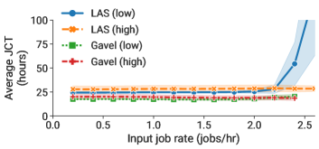
Heterogeneity-Aware Cluster Scheduling Policies for Deep Learning Workloads

Abstract

Specialized accelerators such as GPUs, TPUs, FPGAs, and custom ASICs have been increasingly deployed to train deep learning models. These accelerators exhibit heterogeneous performance behavior across model architectures. Existing schedulers for clusters of accelerators, which are used to arbitrate these expensive training resources across many users, have shown how to optimize for various multi-job, multi-user objectives, like fairness and makespan. Unfortunately, existing schedulers largely do not consider performance heterogeneity. In this paper, we propose Gavel, a heterogeneity-aware scheduler that systematically generalizes a wide range of existing scheduling policies. Gavel expresses these policies as optimization problems, making it easy to optimize for objectives in a heterogeneity-aware way, while also being cognizant of performance optimizations like space sharing. Gavel then uses a round-based scheduling mechanism to ensure jobs receive their ideal allocation given the target scheduling policy. Gavel’s heterogeneity-aware policies allow a heterogeneous cluster to sustain higher input load, and improve end objectives such as average job completion time and makespan by up to 3.5$\times$ compared to heterogeneity-agnostic policies.

1 Introduction

As Moore’s law comes to an end, specialized accelerators such as GPUs, TPUs, FPGAs, and other domain-specific architectures have emerged as an alternative to more general-purpose CPUs. These accelerators have been deployed to great effect [37, 27] to train state-of-the-art deep neural network (DNN) models for many domains, including language, images and video  [57, 15, 32, 33, 53].

Consequently, users today must choose from a wide variety of accelerators to train their DNN models. For example, public cloud users can rent several generations of NVIDIA GPUs and Google TPUs from cloud providers [1, 2, 3]. Even organizations with private clusters have accumulated different accelerator types over time [36]; anecdotally, our research group has Titan V, Titan X, and P100 GPUs in its private cluster. Resources in these multi-tenant settings are typically arbitrated by a scheduler. GPU cluster schedulers such as Themis [42], Tiresias [30], AlloX [39], and Gandiva [60] thus need to decide how to allocate diverse resources to many users while implementing complex cluster-wide scheduling policies, optimizing objectives such as fairness or minimum makespan. Unfortunately, choosing the most effective accelerator types in this context is difficult for three reasons:

(a) Throughput.

(b) Dollar-normalized.

Figure 1: Throughputs and dollar-normalized throughputs of training for various ML models. Dollar-normalized throughputs are computed by dividing the corresponding throughput by the relevant GCP on-demand price, The magnitude of speedup across GPU generations varies significantly across models.

Performance Heterogeneity.

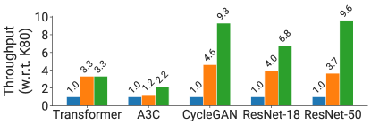
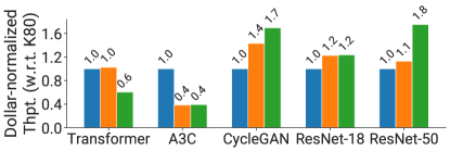
Commonly used model architectures show heterogeneous performance behavior across accelerator types due to various architectural differences. For example, Figure 1(a) shows that a ResNet-50 model sees a nearly 10$\times$ speedup from an NVIDIA V100 GPU compared to a K80 GPU, while an A3C Deep Reinforcement Learning model only sees a 2$\times$ speedup. However, as shown in Figure 1(b), the V100 is no longer the optimal choice for all models when we consider the number of samples trained per dollar – for many models, the older P100 GPU is competitive or cheaper on a per-dollar basis. Some scheduling policies can also benefit from splitting a job between multiple resource types: for example, minimizing a job’s cost subject to a latency SLO (e.g., complete a job in 10 hours) might involve using a cheaper accelerator to begin training and then switching to a faster, more expensive device to meet the SLO. Thus, for even simple single-job settings, the choice of accelerator type is non-trivial and depends on both the job and the policy. This gets more complicated in multi-job settings as granting all jobs their preferred accelerator simultaneously might not be possible. Existing schedulers like Gandiva, Tiresias, and Themis do not consider the heterogeneous performance behavior across accelerators.

Generality Across Policies.

Cluster operators might want to implement different scheduling policies based on their business goals, such as optimizing for time to complete a set of batch jobs (makespan), fairness for ad-hoc jobs, or more sophisticated hierarchical policies that divide resources among high-level entities (e.g., departments) using one policy, and then individual jobs within the entity using another [36]. In data analytics clusters, many job schedulers have support for hierarchical allocation policies [7, 61, 8, 13] already. The two recently proposed GPU schedulers that do consider heterogeneous resources, AlloX [39] and $\text{Gandiva}_{\text{fair}}$ [19], optimize for a single scheduling objective, and tightly couple their scheduling mechanism to that objective (e.g., max-min fairness). Thus, they cannot easily support the more sophisticated policies often used in practice.

Colocation and Placement Optimizations.

To improve cluster utilization, existing GPU schedulers often deploy optimizations such as space sharing as in Gandiva [60], where multiple jobs can use the same accelerator concurrently, and placement sensitivity as in Themis and Tiresias [42, 30], which involves the careful placement of tasks in a distributed job to ensure good scaling performance. The performance benefits of these optimizations should be considered explicitly while optimizing for global scheduling objectives, since these optimizations are more effective when deployed in a heterogeneity-aware way. We show that this explicit modeling for space sharing can improve objectives by up to 2.2$\times$ compared to Gandiva’s ad-hoc approach.

In this paper, we present Gavel, a new cluster scheduler designed for DNN training in both on-premise and cloud deployments, that effectively incorporates heterogeneity in both hardware accelerators and workloads to generalize a wide range of existing scheduling policies. For example, Gavel can provide heterogeneity-aware versions of fair sharing / least attained service [30], FIFO, minimum makespan, minimum cost subject to SLOs, finish-time fairness [42], shortest job first, and hierarchical policies [61, 13].

Gavel’s key observation is that many widely used scheduling policies, including hierarchical ones, can be expressed as optimization problems whose objective is a function of the jobs’ achieved throughputs. For example, least attained service is equivalent to maximizing the minimum scaled throughput among the jobs, makespan is equivalent to minimizing the maximum duration (computed as the ratio of number of iterations to achieved throughput), and so on. Given the optimization problem for a scheduling policy, Gavel introduces a general way to transform the problem to make it heterogenity-, colocation- and placement-aware. In particular, Gavel changes the problem to search over a heterogeneous allocation for each job, the fraction of time spent in various resource configurations (e.g., 60% of time running alone on a V100 GPU and 40% of time space-sharing an A100 GPU with another job), and changes the throughput terms in the objective function to effective throughput, i.e. the average throughput of the job over the mix of resources in its allocation. Additional constraints need to be added to ensure that the returned allocation is valid. We show that Gavel’s transformed optimization problems are efficient to execute even for clusters with hundreds of GPUs and jobs, and can support a wide range of policies. Many of these problems can be solved using a sequence of one or more linear programs.

Gavel’s heterogeneity-aware allocations for each job need to be mapped to actual scheduling decisions (placement of jobs on specific resources in the cluster for a specified duration of time). To achieve this, Gavel uses a preemptive round-based scheduling mechanism to ensure that jobs receive resources in fractions similar to the computed target allocation. Gavel’s scheduling mechanism needs to be able to schedule both distributed training jobs, which request multiple accelerators at once, as well as combinations of jobs running concurrently on a given accelerator due to space sharing.

Gavel makes these scheduling decisions transparently: it specifies an API between the scheduler and applications that allow jobs written in existing deep learning frameworks like PyTorch [50] and TensorFlow [14] to be moved between resources with minimal code changes, and uses a mechanism similar to Quasar [23] to estimate performance measurements of colocated jobs, which are needed as inputs to Gavel’s policies, when not available a priori.

By explicitly considering performance heterogeneity, Gavel improves various policy objectives (e.g., average job completion time or makespan): on a smaller physical cluster, it improves objectives by up to 1.4$\times$, and on a larger simulated cluster, it increases the maximum cluster load, while improving objectives such as average job completion time by 3.5$\times$, makespan by 2.5$\times$, and cost by 1.4$\times$.

To summarize, our main contributions are: 1) A systematic method to convert existing cluster scheduling policies into equivalent policies that consider heterogeneity and colocation; these equivalent optimization problems are practical to execute for current DNN clusters. 2) A round-based scheduling mechanism to ensure that the cluster realizes the allocations returned by these policies. 3) Generalizations of many existing policies in our framework that improve overall performance and other policy objectives by up to 3.5$\times$.

Figure 2: Gavel overview. Jobs are written in frameworks like PyTorch or TensorFlow. Gavel’s throughput estimator obtains performance measurements for each runnable job on each available accelerator type if necessary; its policy then computes an allocation that optimizes a user-specified objective such as fairness. Gavel’s scheduling mechanism accepts this computed allocation as an input, and makes per-round placement decisions in proportions that faithfully mimic the computed allocation.

2 Background

In this section, we provide a brief overview of DNN training (§2.1), and discuss performance optimizations used in existing schedulers that Gavel can help deploy more effectively (§2.2).

2.1 Deep Neural Network (DNN) Training

DNN training proceeds in iterations. In each iteration, the DNN processes a collection of inputs (called a minibatch) and subsequently updates the model parameters using gradients derived from the input minibatch. Each minibatch is typically of similar size, which means model training throughput can be measured by averaging over 100s of iterations. Gavel leverages this fact in its throughput estimator. Jobs are typically fairly long-running (on the order of hours to days), and can be distributed over many workers [10, 60].

Modern DNN schedulers leverage the fact that DNN training is iterative to suspend and resume training at iteration boundaries [30, 60]; this ensures that jobs can be time multiplexed over the existing physical resources. The latest model parameters need to be checkpointed to stable storage when a job is suspended to ensure training progress is not lost.

2.2 Performance Optimizations

Prior work has shown that GPUs can be severely under-utilized in multi-tenant clusters [36]; for example, average GPU utilization (measured as the percentage of GPU Streaming Multiprocessors active over time) was as low as $52\%$ on a Microsoft cluster. Prior work has also shown the placement of tasks for a distributed training job can have significant impact on performance. Gavel can more systematically employ these optimizations, as we show in §3.1.

Space Sharing.

Smaller models often do not leverage the full computational capacity of modern GPUs. In such cases, concurrently executing multiple models on the same GPU using NVIDIA’s Multi Process Service (MPS) or CUDA streams can help improve utilization [11, 49].

Placement Sensitivity.

DNN models show heterogeneity in their distributed scaling behavior depending on the size of the data that need to be exchanged between workers during training: some models have compact weight representations and can scale well even when workers are not on the same server, while other models scale poorly when workers are spread over many servers. Existing schedulers like Tiresias use heuristics for placement sensitivity to ensure that model training is run in a consolidated setting when necessary.

3 Overview of Gavel

Given a collection of jobs, Gavel arbitrates cluster resources (in the form of accelerators of different types) among the resident jobs, while optimizing for the desired cluster objective. This is accomplished in a two-step process: first, a heterogeneity-aware policy computes the fraction of time different jobs (and combinations) should run on different accelerator types to optimize the desired objective. These policies require as input the performance behavior (in terms of throughputs) for each job on each accelerator type, which can either be provided by the user, or can be measured on the fly by Gavel’s throughput estimator. Then, given the policy’s output allocation, Gavel’s scheduling mechanism grants jobs time on the different resources, and moves jobs between workers as necessary to ensure that the true fraction of time each job spends on different resources closely resembles the optimal allocation returned by the policy. Gavel can recompute its policy either when a reset event occurs (job arrives or completes, or a worker in the cluster fails), or at periodic intervals of time. Gavel’s workflow is shown in Figure 2.

3.1 Heterogeneity-Aware Policies

Gavel expresses scheduling policies as optimization problems for various objectives of interest, such as fairness or makespan, and allocations as matrices that specify the fraction of wall-clock time a job should spend on each accelerator type. A matrix $X$ can represent allocations on a single accelerator type (homogeneous setting), allocations on multiple accelerator types (heterogeneous setting), as well as allocations with other optimizations deployed. For three jobs and three accelerator types, an example allocation could be:

$$X^{\text{example}}=\blockarray{cccc}V100&P100K80\\ \block{(ccc)c}0.60.40.0\text{job 0}\\ 0.20.60.2\text{job 1}\\ 0.20.00.8\text{job 2}\\$$

Figure 3: The cumulative time each job spends on accelerator types between allocation recomputations for allocation $X^{\text{example}}$.

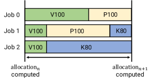
According to this allocation, job 0 should spend 60% of its time on a V100 GPU, and job 1 should spend 40%. This is shown visually in Figure 3.

Gavel finds an optimal value for the matrix $X$ given a policy expressed as an optimization problem. To construct the optimization problem for a given policy, Gavel requires a throughput matrix $T$ with each job’s throughput (in training iterations per second) on different accelerators. $T_{mj}$ can be set to $-\infty$ if job $m$ does not run on accelerator type $j$ (for example, due to memory constraints).

Given $T$ and $X$, we define the effective throughput of a model $m$ as the time-weighted average throughput across accelerators and jobs. We denote this quantity $\text{\text{throughput}}_{T}(m,X)$ or simply $\text{\text{throughput}}(m,X)$ (dropping the $T$) for brevity. For allocations $X$ without space sharing,

$$\text{throughput}(m,X)=\sum_{\begin{subarray}{c}j\in\\ \text{accelerator types }\end{subarray}}T_{mj}\cdot X_{mj}$$

Different cluster scheduling policies can be expressed as optimization problems for $X$ while maximizing or minimizing an appropriate objective function. Constraints need to be specified to ensure that $X$ is a valid allocation. Then, a hypothetical policy that maximizes total effective throughput would look like,

$$\text{Maximize}_{X}\sum_{m\in\text{jobs}}\text{throughput}(m,X)$$

We need to add additional constraints to ensure that the cluster is not overprovisioned:

$$0\leq X_{mj}\leq 1 \forall(m,j)$$ (1)

$$\sum_{j}X_{mj}\leq 1 \forall m$$ (2)

$$\sum_{m}X_{mj}\cdot\text{scale\_factor}_{m}\leq\text{num\_workers}_{j} \forall j$$ (3)

These constraints ensure that each job-worker allocation is non-negative and is between $0$ and $1$, that the total allocation for a job does not exceed 1, and that the allocation does not oversubscribe the workers.

Space Sharing.

Gavel’s allocation matrices can also incorporate space sharing options. While previous work has used greedy algorithms for space sharing, we found that different pairs of DNN applications in practice have vastly different performance when colocated together, based on the resources they consume (Figure 15 in Appendix). When using space sharing, $X$ needs to contain rows for each viable combination of jobs, and $T$ needs to have throughputs of the job combinations, like:

$$T=\blockarray{cccc}V100&P100K80\\ \block{(ccc)c}4.02.01.0\text{job 0}\\ 3.02.01.0\text{job 1}\\ (2.0,1.5)0.00.0\text{jobs (0, 1)}\\$$

We limit entries of $T$ to combinations of at most 2 jobs; we found empirically that larger combinations rarely increase net throughput. Additionally, although the size of $T$ grows quadratically with the number of jobs even with job combinations of size 2, we found that in practice we only need to consider combinations that actually perform well. We evaluate the scaling behavior of these SS-aware policies in §7.4.

Objectives in terms of $\text{throughput}(m,X)$ remain the same; however, $\text{throughput}(m,X)$ now needs to be computed to include the throughputs of co-located jobs, and additional constraints need to be specified to ensure that $X$ is a valid allocation in this new regime:

$$0\leq X_{kj}\leq 1 \forall k,j$$

$$\sum_{k\in C_{m}}\sum_{j}X_{kj}\leq 1 \forall m$$

$$\sum_{k}X_{kj}\cdot\text{scale\_factor}_{m}\leq\text{num\_workers}_{j} \forall j$$

$C_{m}$ is the set of all job combinations that contain job $m$.

Placement Sensitivity.

Similarly, Gavel’s allocation matrices can also be extended to incorporate placement sensitivity. The observed throughput for distributed jobs depends on the location of tasks, as well as the model and accelerator type (slower workers are less likely to be communication-bound, which means consolidation of tasks is less effective). We can make our policies placement-sensitive by considering the performance of distributed jobs in: 1) a consolidated setting, where as many accelerators are on the same server as possible (for example, 8 GPUs per server if using 8-GPU servers), and 2) an unconsolidated setting, where accelerators are on independent servers. These are extreme points in the placement space, and are upper and lower bounds on performance. We can model this in our policies by having two different worker types (consolidated and unconsolidated) with corresponding throughput values in $T$ and allocation values in $X$.

Figure 4: Priorities are used to move the received allocation towards the intended allocation (in this case, $X^{\text{example}}$). $\text{priorities}_{n}$ is computed as $f(X,\text{rounds\_received}_{n})$ where $f(.)$ is the element-wise division operator.

3.2 Round-based Scheduling Mechanism

After computing the optimal allocation, Gavel’s next step is to assign jobs (or job combinations, in the case of space sharing) to accelerator types while matching the optimal allocation as closely as possible. That is, to realize the allocation $X^{\text{example}}$ above, the scheduling mechanism needs to make sure that in the time period where jobs 0, 1, and 2 are the only three runnable jobs in the cluster, jobs should receive resources according to their computed fractions (e.g., job 0 receives 60% of V100 time).

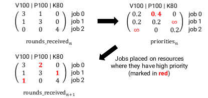
To do this, the scheduler computes a priority score for every job and accelerator type combination that is high when a job has received a smaller time fraction than the optimal allocation. Scheduling is performed in rounds; in each round, the scheduler runs jobs in decreasing priority order, while ensuring that a given job is not scheduled on multiple workers (or accelerators) in a given round. This is shown in Figure 4. Priorities are updated as rounds complete. We have found empirically that round durations of 20 minutes or less allow Gavel to effectively approximate the ideal allocation. We present an analysis of how the round duration affects scheduling quality and overhead in §7.5.

3.3 Throughput Estimator

To estimate the throughputs of concurrent jobs (e.g., in the case of space sharing), Gavel employs a throughput estimator, similar to those found in prior work such as Quasar [23]. Gavel’s throughput estimator maps a new job to a set of pre-profiled reference jobs. The throughputs of the closest reference job can then be used as the initial performance estimate for the new job’s combinations. For individual jobs, the throughput estimator is not needed, since these can be estimated on the fly as jobs run on different resource types over many rounds.

3.4 Limitations and Non-Goals

While Gavel exposes a flexible API that supports a variety of policies and objectives, we do not propose new scheduling policies or performance optimizations in this work. Instead, Gavel’s main goal is to determine how best to share resources amongst many different users and jobs in a heterogeneity-aware way, while supporting many existing cluster-wide objectives. Gavel accomplishes these goals with a policy framework that easily allows policies to be made heterogeneity-, colocation-, and placement-aware (§4), a scheduling mechanism that can be reused across policies (§5), and a narrow scheduler API that allows users to deploy their applications on the shared cluster with minimal code changes (§6).

4 Scheduling Policies

In this section, we show how various scheduling policies such as max-min fairness (Least Attained Service or LAS) and multi-level fairness can be expressed as optimization problems in terms of effective throughput. We also describe some properties of the resulting heterogeneity-aware allocations at the end of this section.

4.1 Max-Min Fairness as an Optimization Problem

The classical Least Attained Service (LAS) policy, used by Tiresias [30], implements max-min fairness across active users in the cluster, by round-robining resources across jobs according to the total number of accelerator hours consumed. This can be modified into a weighted max-min fairness policy with per-user weights $w_{m}$.

Thus, on a homogeneous cluster, if a job $m$ with weight $w_{m}$ receives a fraction $X_{m}$ (which is a scalar since there is only one resource type), LAS can be expressed as the following optimization problem:

$$\text{Maximize}_{X}\min_{m}\dfrac{1}{w_{m}}X_{m}$$

We need to add an additional constraint to ensure that the cluster is not overprovisioned ($\sum_{m}X_{m}\leq 1$).

However, this vanilla LAS policy is not fair in a heterogeneous setting; jobs might see unequal reductions in throughput due to variations in performance across accelerator types. For example, giving one job a K80 and another job a V100 would equalize their number of resources, but could result in very low performance for the job with the K80.

To compute a more fair allocation, we can compute max-min fairness over the weighted normalized effective throughputs, as defined in §3.1. Let $X_{m}^{\text{equal}}$ be the allocation given to job $m$ assuming it receives equal time share on each worker in the cluster. For example, if the cluster had 1 V100 and 1 K80, $X_{m}^{\text{equal}}=[0.5,0.5]$. $X_{m}^{\text{equal}}$ scales the effective throughputs to make them comparable across jobs.

$$\text{Maximize}_{X}\min_{m}\dfrac{1}{w_{m}}\dfrac{\text{throughput}(m,X)}{\text{throughput}(m,X_{m}^{\text{equal}})}$$

As specified in §3.1, additional constraints need to be specified to ensure that allocations are valid.

As an example, consider 3 jobs which benefit differently when moved from a K80 GPU to a V100 GPU:

$$T=\blockarray{ccc}V100&K80\\ \block{(cc)c}4.01.0\text{job 0}\\ 3.01.0\text{job 1}\\ 2.01.0\text{job 2}\\$$

Solving the above optimization problem with $w_{m}=1$, and a cluster with 1 V100 and 1 K80 yields the following allocation:

$$X^{\text{het.}}=\blockarray{ccc}V100&K80\\ \block{(cc)c}0.450.0\text{job 0}\\ 0.450.09\text{job 1}\\ 0.090.91\text{job 2}\\$$

Jobs receive about 10% higher throughput compared to an allocation where every user is given $1/n$ of the time on each accelerator (in this case, $n=3$), also called an isolated allocation [28].

Fairness policy objective functions need to be modified to take into account muti-resource jobs with $\text{scale\_factor}_{m}>1$, since these multi-resource jobs occupy a larger share of the cluster per unit time. An easy way to do this is to multiply the $\text{scale\_factor}_{m}$ to the max-min objectives from before. Concretely, the LAS objective from before now becomes,

$$\text{Maximize}_{X}\min_{m}\dfrac{1}{w_{m}}\dfrac{\text{throughput}(m,X)}{\text{throughput}(m,X_{m}^{\text{equal}})}\cdot\text{scale\_factor}_{m}$$

4.2 Other Policies as Optimization Problems

Policy	Description
Makespan	Minimize time taken by batch of jobs.
LAS [30]	Max-min fairness by total compute time.
LAS w/ weights	Max-min fairness with weights.
Finish Time Fairness [42]	Maximize minimum job speedup.
FIFO	First in, first out.
Shortest Job First	Minimize time taken by shortest job.
Minimize cost	Minimize total cost in public cloud.
Minimize cost w/ SLOs	Minimize total cost subject to SLOs.
Hierarchical [61]	Multi-level policy: FIFO, fairness, etc.

Table 1: Policies that can be expressed in Gavel.

We can express many other common cluster scheduling policies, some proposed by recent papers, using $\text{\text{throughput}}(m,X)$; we list these policies in Table 1. Most of these policies can be expressed using a single linear program, with a few exceptions: the makespan policy is formulated as a sequence of linear programs, and the cost policies are formulated as a linear-fractional program [9], which can be reduced to a sequence of linear programs as well. These optimization problems yield corresponding heterogeneity-aware allocations. The optimal allocation can be computed by solving one or more linear programs (LP), which off-the-shelf solvers can solve very quickly even at the scale of a large cluster.

Minimize Makespan.

The Minimum Makespan policy tries to complete all active jobs as soon as possible. Gandiva uses a version of this policy to finish higher-level tasks such as hyperparameter tuning and AutoML, which involve training a large number of variants of a model. If $\text{num\_steps}_{m}$ is the number of iterations remaining to train model $m$, then the makespan is the maximum of the durations of all active jobs, where the duration of job $m$ is the ratio of the number of iterations to $\text{throughput}(m,X)$ (which is expressed in iterations / second). Overall, this can be framed as,

$$\text{Minimize}_{X}\max_{m}\dfrac{\text{num\_steps}_{m}}{\text{throughput}(m,X)}$$

Minimize Finish-Time Fairness (Themis).

Themis [42] proposes a new metric called finish-time fairness (represented as $\rho$), which is the ratio of the time taken to finish a job using a given allocation and the time taken to finish the job using $1/n$ of the cluster ($X^{\text{isolated}}$), assuming $n$ users using the cluster. This can be expressed in terms of $\text{throughput}(m,X)$ as follows ($\text{num\_steps}_{m}$ is the number of iterations remaining to train model $m$, $t_{m}$ is the time elapsed since the start of training for model $m$, and $t^{\text{isolated}}_{m}$ is the hypothetical time elapsed since the start of training if model $m$ had a dedicated fraction of the cluster to itself),

$$\rho_{T}(m,X)=\dfrac{t_{m}+\frac{\text{num\_steps}_{m}}{\text{throughput}(m,X)}}{t^{\text{isolated}}_{m}+\frac{\text{num\_steps}_{m}}{\text{throughput}(m,X^{\text{isolated}})}}$$

The final optimization problem is then,

$$\text{Minimize}_{X}\max_{m}\rho_{T}(m,X)$$

FIFO.

The First-In-First-Out (FIFO) policy schedules jobs in the order they arrive. In a heterogeneous regime, jobs should be placed on the fastest available accelerator type. Mathematically, we can write this as maximizing the throughput of job $m$ relative to its throughput on the fastest type ($\text{throughput}(m,X^{\text{fastest}})$). Assuming that jobs are enumerated in order of their arrival time ($m$ arrived before $m+1$), a FIFO allocation can be computed with the following objective:

$$\text{Maximize}_{X}\sum_{m}\frac{\text{throughput}(m,X)}{\text{throughput}(m,X^{\text{fastest}})}(M-m)$$

where $M$ is the total number of jobs.

Shortest Job First.

The Shortest Job First policy finds the allocation that minimizes the duration of the shortest job,

$$\text{Minimize}_{X}\min_{m}\dfrac{\text{num\_steps}_{m}}{\text{throughput}(m,X)}$$

Minimizing Total Cost and Cost subject to SLOs.

We can express policies for deployments that use elastic public cloud resources. Since cloud VMs are charged on a per-time basis, we can express policies that explicitly optimize for total cost, speed, or both.

Consider a simple policy that maximizes total throughput,

$$\text{Minimize}_{X}\sum_{m}\text{throughput}(m,X)$$

The above policy can be extended to incorporate cost by optimizing the following cost-adjusted objective,

$$\text{Maximize}_{X}\frac{\sum_{m}\text{throughput}(m,X)}{\sum_{m}(\sum_{j}\text{cost}_{j}\cdot X_{mj})}$$

where $\text{cost}_{j}$ is the cost of accelerator type $j$. The numerator in the above objective is the time-averaged effective throughput, and the denominator is the time-averaged cost. When using space sharing, care must be taken to not double count the cost of instances running job combinations (all jobs in a job combination derive value in terms of some throughput from the instance).

Jobs can have time SLOs as well, e.g., certain high-priority jobs might need to complete every 12 hours. We can add additional constraints: given $\text{SLO}_{m}$ for each model $m$ (models without SLOs can have $\text{SLO}_{m}=\infty$),

$$\text{throughput}(m,X)\geq\text{num\_steps}_{m}/\text{SLO}_{m}$$

4.3 Hierarchical Scheduling Policies

Figure 5: Example of a hierarchical policy: weighted fairness across two entities: a product and research team, fairness across jobs within the product team, and FIFO within the research team.

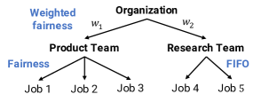
Modern cluster schedulers do not only deploy “single-level” policies. Hierarchical policies are common [7, 61, 13]: a large organization might share a single physical cluster among many sub-organizations (or entities) using a fairness policy. In turn, each entity can share resources among individual jobs according to a distinct per-entity policy, such as per-user fairness or FIFO. We give an example in Figure 5, where a research and product team share the same physical cluster. The research team runs ad-hoc experiments that can be executed in FIFO order, but the product team needs to ensure that all its jobs receive a fair share of the cluster.

Gavel can currently support fairness in the upper levels and fairness or FIFO in the lower levels, which matches the hierarchical policies supported by the Hadoop scheduler [7]. Determining how to extend this to other hierarchical policy sets (for example, with finish time fairness) is future work.

Gavel solves hierarchical objectives using a procedure called water filling [16], which is used in other max-min fairness problems such as link allocation in networks [51]. At a high level, the water-filling algorithm increases the allocation given to all parties at an equal rate to respect max-min fairness, until a party saturates. The saturated party is then taken out, and the procedure repeated iteratively until all commodities are saturated. We adapt this procedure to our setting, solving a series of optimization problems iteratively: an LP that computes a fair allocation across entities while respecting each entity’s internal policy, and an MILP (specified in Appendix A.1) that identifies bottlenecked jobs, i.e., jobs whose effective throughputs cannot be improved without lowering the effective throughput of other jobs.

We denote each entity $s$ associated with a weight $w_{s}$; the jobs belonging to this entity receive a total share of the cluster proportional to this weight. We denote $w^{\text{job}}_{m}$ to be the weight of job $m$, set such that $\sum_{m\in s}w^{\text{job}}_{m}=w_{s}$. Jobs are assigned priorities in accordance to the relevant entity’s policy; for example, a fairness policy at the entity level would assign each job a weight proportional to its individual weight within the entity, while for FIFO, the first job in the queue would initially receive the entire weight of the entity.

In each iteration, we solve the following modified LP, assuming $\text{scale\_factor}_{m}=1$ for all $m$ for simplicity:

$$\text{Maximize}_{X}\min_{\{m:w^{\text{job}}_{m}>0\}}\frac{1}{w^{\text{job}}_{m}}\bigg{(}\frac{\text{throughput}(m,X)}{\text{throughput}(m,X_{m}^{\text{equal}})}-t_{m}\bigg{)}$$

$t_{m}$ is the normalized effective throughput of job $m$ in the previous iteration ($t_{m}:=0$ in the first iteration). The above objective can be appropriately modified for larger $\text{scale\_factor}_{m}$. Bottlenecked jobs are given priority 0 and no longer considered in future iterations. Priorities are redistributed among non-bottlenecked jobs according to the entity’s policy at the end of every iteration. For instance, in the example shown in Figure 5, if job 4 is bottlenecked then its weight is reassigned to job 5 in accordance to the FIFO policy, while if job 2 is bottlenecked, its weight is distributed equally between jobs 1 and 3 in accordance with the entity’s fairness policy. The LP then solves the max-min problem on the resources remaining while ensuring each job’s throughput does not drop compared to the previous iteration’s allocation $X^{\text{prev}}$, expressed as the constraint $\text{throughput}(m,X)\geq\text{throughput}(m,X^{\text{prev}})$ for all m.

Iterations continue until all jobs are bottlenecked. To make this procedure more concrete, consider an example with 4 identical jobs: job 1 with a weight of 3.0, and jobs 2-4 with a weight of 1.0; and 4 identical GPUs. In the first iteration, job 1 is assigned resources such that its throughput is 1.0, and jobs 2, 3, and 4 are assigned resources such that their throughput is 0.33 to respect weights. Job 1 is a bottleneck; the throughput of the remaining jobs can still be increased. In the next iteration, jobs 2-4 are given full-GPU allocations.

The final allocation satisfies both inter-entity and intra-entity policies. We note that the above water-filling procedure can also be used for single-level fairness policies such as the one described in §4.1 to improve the throughput of non-bottelenecked jobs.

4.4 Properties of Gavel’s Policies

Existing scheduling schemes have been analyzed in terms of properties like sharing incentive, Pareto efficiency, and strategy proofness [28]. We formalize Gavel’s heterogeneity-aware policies in the context of these properties as well.

Homogeneous Clusters.

For homogeneous clusters, Gavel’s heterogeneity-aware policies are equivalent to the baseline policies ($\text{throughput}(m,X)=X_{m}\cdot T_{m}$), since the heterogeneity-aware optimization problems reduce to the original optimization problems with one accelerator type.

Sharing Incentive.

For heterogeneous clusters, the policy’s objective metric (maximize least job share in LAS, completion time of first job in FIFO, or makespan) is at least as well off as it would be under a policy that naïvely splits all resources equally among all runnable jobs. This is because the allocation corresponding to giving each user $1/n$ of each resource is a feasible solution to Gavel’s optimization problem, so Gavel’s solution will be at least as good. All Gavel policies have sharing incentive [28], which encourages users to use the shared cluster rather than a static private share.

Colocation.

Solutions with colocation are always at least as good as without colocation.

Pareto Efficiency.

Allocations of max-min fairness policies with water filling are Pareto efficient: that is, the allocation for a particular job cannot be increased without decreasing the allocation for another job.

Note that some of Gavel’s policies may not satisfy other desirable properties. For example, Sun et al. [55] showed that no fair-sharing policy can simultaneously satisfy Pareto efficiency, sharing incentive and strategy proofness in a setting with interchangeable resources. We leave consideration of strategy-proof policies to future work.

5 Scheduling Mechanism

Gavel’s scheduling mechanism schedules training iterations of runnable jobs on the available workers (with possibly different accelerators), such that for each schedulable job (or combination), the fraction of wall-clock time it spends on each device class is approximately equal to the computed optimal allocation $X^{\text{opt}}$ between allocation recomputation events. This is challenging for two main reasons: 1) Jobs can run on multiple accelerators. Moreover, since distributed training can be communication intensive [21, 48], jobs should be placed on accelerators “close” to each other (for example, on accelerators on the same server, or on accelerators in servers in the same rack). 2) Combinations of up to two jobs can run on a set of accelerators in order to improve resource utilization (space sharing). Each distinct job can have $\leq 1$ job combination running in a given round to prevent work duplication.

Gavel makes its scheduling decisions in rounds. That is, the scheduler tries to place work on all available workers for a specific duration (this time period is configurable; we use 6 minutes in our experiments). We call the work handed to each worker in a given round a micro-task. Without rounds, jobs that request many accelerators can suffer from starvation. For example, consider a cluster with 8 total accelerators and 4 available. The scheduler can handle a 8-accelerator job waiting for resources in one of two ways: a) wait for 8 accelerators to become available; 4 accelerators will be unused until the full quota of 8 accelerators becomes available, b) keep the 8-accelerator job in the queue, and give 4 accelerators to another job that requests a fewer number of resources. However, this situation can repeat itself, leading to starvation [61]. Scheduling is thus performed in rounds to limit resource under-utilization that can arise from starvation mitigation, simplify scheduling logic, and still ensure that jobs that request a large number of workers do not experience prolonged starvation.

Since the number of active, schedulable jobs might far exceed the total number of workers, Gavel first determines the job combinations that should run in the upcoming round. To do this, Gavel maintains the time $t_{mj}$ spent by a job (or combination) $m$ on accelerator type $j$, which is updated as jobs run on different accelerator types every round. Given $t_{mj}$, Gavel’s scheduler can then compute the fraction of total wall-clock time spent by each job (or combination) $m$ on each accelerator type $j$ as $f_{mj}=t_{mj}/(\sum_{m^{\prime}}t_{m^{\prime}j})$. The matrix of priorities is then just the element-wise division of $X^{\text{opt}}$ by $f$.

Algorithm.

In every round, we want to move $f_{mj}$ closer to $X^{\text{opt}}_{mj}$. This can be achieved by giving high-priority jobs time on accelerator type $j$.

This problem can be solved exactly if jobs only request single accelerators and if space sharing is not deployed, by finding the $\text{num\_workers}_{j}$ jobs with highest priority (for example, using a heap). However, jobs submitted to Gavel can be distributed, and space sharing can be used to improve resource utilization. Solving this problem exactly with these added requirements makes the problem similar to a multiple-choice knapsack problem [54], which is NP-hard.

Figure 6: Round-based scheduling mechanism in action to achieve an allocation $X^{\text{het.+SS}}$. Space sharing is shown with vertically split boxes. Each round is denoted by a box. Numbers in boxes represent Job IDs.

To overcome these challenges, we observe that it is acceptable to make greedy sub-optimal decisions occasionally, since we can recover from these sub-optimal decisions in subsequent rounds. We study the impact of this design choice in §7.5. A job not run in a particular round will have increased priority in subsequent rounds until it receives accelerator time, while a job combination that runs in a particular round will have decreased priority. This ensures that job combinations cannot suffer from starvation if they have a non-zero optimal allocation (priority $>0$).

Algorithm 1 Algorithm for Gavel’s scheduling mechanism

1:function schedule_jobs

2:    active_combinations $\leftarrow$ all active job combinations

3:    num_workers_remaining $\leftarrow$ number of total workers

4:    while num_workers_remaining $>0$ do

5:         $j$ $\leftarrow$ job combination with highest priority

6:         Remove $j$ from active_combinations

7:         if $j$.scale_factor $>$ num_workers_remaining then

8:             continue          

9:         for all $j^{\prime}$ that conflict (share a job $k$) with $j$ do

10:             Remove $j^{\prime}$ from active_combinations          

11:         num_workers_remaining $-=j$.scale_factor     

Gavel uses a greedy algorithm to pick the highest-priority job combinations that fit in the provided resource budget. The algorithm maintains a set of eligible job combinations (eligible_job_combinations) that can be scheduled in the upcoming scheduling round. The scheduling mechanism then tries to add job combinations with highest priority into a job_combinations_to_schedule set. Once a job combination is added to this set, all conflicting job combinations are removed from the set of eligible combinations to ensure that a given job is not run more than once in a given scheduling round. Job combinations that cannot fit in the current round due to space limitations (required number of accelerators scale_factor unavailable) are also removed from the set of eligible combinations. This algorithm is detailed in Algorithm 1. Gavel’s scheduling mechanism is decoupled from its policies, ensuring that the same scheduling mechanism can be used for many different policies. Figure 6 shows Gavel’s scheduling mechanism in action.

Once Gavel has decided what jobs (and combinations) should run in a given round on different accelerator types, Gavel must decide how to place these jobs. Gavel’s scheduler places jobs in decreasing order of the number of requested workers, and tries to give jobs accelerators on the same physical server to minimize fragmentation.

6 Implementation

We implemented a prototype of Gavel and an accompanying simulator in approximately 8000 lines of Python code. We used cvxpy [25] to implement Gavel’s heterogeneity-aware policies, and gRPC [5] for the communication of control messages between the scheduler and workers.

Interface between Scheduler and Applications.

Gavel currently supports user applications written in PyTorch [50]; support for TensorFlow [14] is left for future work. The scheduler and user applications then interact through a narrow API. Gavel ships with a Python library that users can import into their code. This library provides an implementation for a GavelIterator, a wrapper around existing framework-provided data iterators. The GavelIterator ensures that each task in a distributed job runs for the same number of iterations, and synchronizes the conclusion of rounds between the scheduler and workers. GavelIterator is instantiated with load_checkpoint and save_checkpoint function pointers, which can be called to load all necessary parameters and metadata from a checkpoint at the start of a round, and to create a checkpoint at the end of a round. Both the load_checkpoint and save_checkpoint methods need to be implemented by the user, but only need to call appropriate framework methods (about 10 LOC in our implementation). GavelIterator contacts the scheduler near the end of a round to see if the same job will run in the next round on the same worker. We call this a lease renewal. If the lease is not renewed, the iterator calls the save_checkpoint method at the end of the round, and returns execution back to the scheduler. The scheduler can then launch another job on the worker.

Throughput Estimation.

Figure 7: Gavel’s throughput estimator. Profiling is combined with matrix completion to obtain a fingerprint for every new job. The fingerprint is then used to find the closest reference job.

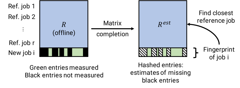
Gavel uses a similar technique to Quasar [23] to estimate colocated throughputs when space sharing if they are not available a priori, mixing profiling with matrix completion. Matrix completion enables sparse low rank matrices to be reconstructed with low error [45, 18]. With matrix completion, Gavel is able to extrapolate measurements obtained through direct profiling on separate workers dedicated to profiling, and determine the job’s most similar pre-profiled reference job. The throughput estimator can then use the reference job’s throughput measurements as an initial throughput estimate. Gavel’s throughput estimator is diagrammed in Figure 7.

Model	Task	Dataset / Application	Batch size(s)
ResNet-50 [33, 6]	Image Classification	ImageNet [24]	16, 32, 64, 128
ResNet-18 [33, 41]	Image Classification	CIFAR-10 [38]	16, 32, 64, 128, 256
A3C [46, 29]	Deep RL	Pong	4
LSTM [12]	Language Modeling	Wikitext-2 [44]	5, 10, 20, 40, 80
Transformer [57, 35]	Language Translation	Multi30k [26] (de-en)	16, 32, 64, 128, 256
CycleGAN [62, 40]	Image-to-Image Translation	monet2photo [62]	1
Recoder [47] (Autoencoder)	Recommendation	ML-20M [31]	512, 1024, 2048, 4096, 8192

Table 2: Models used in evaluation.

Trace	System	Objective	Physical	Simulation
Continuous	Gavel	Average JCT	3.6 hrs	3.4 hrs
Continuous	Baseline LAS	Average JCT	5.0 hrs	5.2 hrs
Static	Gavel	Makespan	17.7 hrs	17.9 hrs
Static	Gandiva	Makespan	21.3 hrs	21.9 hrs

Table 3: Comparison of end objective between physical experiment and simulation for two different traces. For the continuous trace, we measure the average JCT of 25 jobs in a steady-state cluster. For the static trace, we measure the total time needed to complete 100 jobs submitted at the start of the run. The heterogeneity-aware policies improve target objectives by up to 1.4$\times$, and results on the physical cluster are in agreement with results on simulated cluster ($<5\%$).

(a) Average job completion time vs. cluster load.

(b) CDF of job completion times.

Figure 8: Comparison of heterogeneity-agnostic least attained service (LAS) policy to a heterogeneity-aware LAS policy, on the simulated cluster and continuous-single trace.

7 Evaluation

In this section, we seek to answer the following questions:

• Do Gavel’s heterogeneity-aware policies improve objective metrics in a physical cluster (§7.2) and in simulations of larger clusters (§7.3)?

• How does Gavel’s scheduling overhead scale with the number of active jobs? (§7.4)

• How well does Gavel’s scheduling mechanism realize Gavel’s heterogeneity-aware allocations? (§7.5)

• Is Gavel able to accurately estimate the throughputs of co-located jobs when using space sharing? (§7.6)

7.1 Experiment Setup

We run experiments on both a physical and simulated cluster.

Clusters.

We run physical cluster experiments on a 48-GPU cluster with 8 V100s, 16 P100s, and 24 K80s. Simulated cluster experiments are run on a 108-GPU cluster with 36 V100s, 36 P100s, and 36 K80s.

Traces.

We run physical and simulated experiments on two types of traces: one where all jobs are available at the start of the trace and jobs are not subsequently added (“static”), and another where jobs are continuously added to the cluster (“continuous”).

For the continuous trace, job arrival times are generated according to a Poisson arrival process initialized with an inter-arrival rate $\lambda$. For the simulated experiments, we vary $\lambda$ to show the extra load each Gavel policy is able to sustain in steady state. We run 3 seeds for every $\lambda$, and show standard deviations. For the physical cluster experiments, we use a single $\lambda$ that keeps the cluster well-utilized in steady state.

Traces are populated with a list of 26 job configurations, including CNN-based image classification models, RNN-based language models, and others, based on performance measurements on real hardware. Table 2 presents the full list of models and configurations. We sample durations from an exponential distribution between $10^{1.5}$ minutes and $10^{4}$ minutes to match the process Gandiva used in its evaluation [60]. For the simulated experiments, we show results in two regimes: one where all jobs use a single worker (“continuous-single”), and another where roughly 70% of jobs request a single worker, another 25% request between 2 and 4 workers, and the remaining 5% request 8 workers, as observed in published traces from Microsoft [10] (“continuous-multiple”).

Metrics.

For fairness and FIFO policies, our target metric is average job completion time of steady-state jobs, which is the same metric used by related work [43, 30]. We also show finish time fairness (FTF) for policies that explicitly optimize for FTF. For makespan policies, our target metric is the time needed to complete a batch of jobs, and only the static trace is used. For cost-related policies, the metric is cost (in dollars), and the percentage of jobs that violate SLOs.

Round durations.

For the results presented in §7.2, we use a round duration of 20 minutes, and for all other results we use a round duration of 6 minutes (we explain the choice of 6 minutes in §7.5). We use a larger duration in the physical cluster experiments to mitigate scheduler overhead; however, previous work has shown that it is feasible to hide this overhead [60, 42, 4, 20]. We also found that using 6 minute rounds in simulation for the §7.2 experiments did not significantly alter the results.

(a) Average job completion time vs. cluster load.

(b) CDF of job completion times.

Figure 9: Comparison of heterogeneity-agnostic least attained service (LAS) policy to a heterogeneity-aware LAS policy, on the simulated cluster and continuous-multiple trace. Each input job rate is run with 3 seeds; shaded regions around lines show the standard deviati/n.

7.2 End-to-End Results on Physical Cluster

For our physical cluster experiments, we run a heterogeneity-aware and a heterogeneity-agnostic fairness policy on an appropriately-sized continuous trace, and a heterogeneity-aware makespan policy against a baseline that uses Gandiva’s ad-hoc space sharing on an appropriately-sized static trace. Results are shown in Table 3. Gavel’s heterogeneity-aware policies help improve objectives by up to 1.4$\times$.

We also compare the real performance to simulations and observe that for both policies, the difference between metrics in simulation and on the physical cluster is small ($<5\%$), indicating that our simulator has high fidelity.

7.3 End-to-End Results in Simulation

We use a larger simulated cluster to evaluate the efficacy of Gavel’s heterogeneity-aware policies across a range of objectives, and compare with heterogeneity-agnostic versions from previous work. As appropriate, we compare to other baselines like AlloX. We include additional supporting figures in the Appendix (§A.2).

Least Attained Service (LAS).

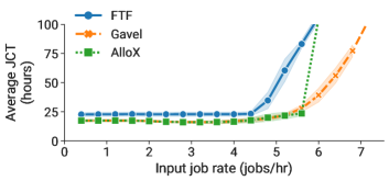
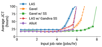
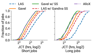
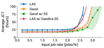
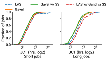
Figures 8 and 9 compare the vanilla LAS policy with its heterogeneity-aware variants. We compare with two other baselines: a modified LAS policy that uses Gandiva’s ad-hoc space sharing, and an AlloX policy that explicitly optimizes average job completion time (but only for single-worker jobs). We make three observations.

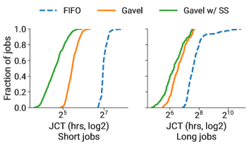
First, the heterogeneity-aware policies support higher load on the same cluster, and also reduce average JCT by up to 3.5$\times$ for the single-worker trace, and by up to 2.2$\times$ for the multi-worker trace. Second, the heterogeneity-aware LAS version supports higher load than AlloX, since AlloX can give short jobs preferential treatment in the interest of optimizing average JCT, leading to long jobs experiencing starvation (long tail in long jobs CDF). At moderate load, AlloX represents a best-case scenario since it explicitly optimizes for average JCT on a heterogeneous cluster. Gavel is able to essentially match AlloX on average JCT, while also being able to support other objectives. Third, Gandiva-style packing, which randomly explores job combinations until a combination that improves performance is found, is ineffective compared to the principled packing used by Gavel’s heterogeneity-aware policies (2.2$\times$ better average JCT for both traces).

(a) Average job completion time vs. cluster load.

(b) CDF of perf-job FTF.

Figure 10: Comparison of heterogeneity-agnostic finish time fairness (FTF) policy to a heterogeneity-aware FTF policy, on the simulated cluster and continuous-multiple trace.

Finish Time Fairness (FTF).

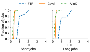
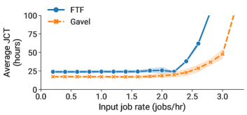
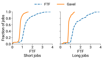
We compare the heterogeneity-aware version of Finish Time Fairness (FTF) to its heterogeneity-agnostic counterpart in Figure 10. The heterogeneity-aware policy reduces average JCTs by 3$\times$ and improves average FTF by 2.8$\times$.

Makespan.

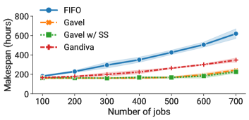
Gavel’s heterogeneity-aware makespan policy reduces makespan by 2.5$\times$ compared to a FIFO baseline, and by 1.4$\times$ compared to a baseline that uses Gandiva’s ad-hoc space sharing. Makespan is reduced by a further 8% when the number of jobs in the trace is high when using space sharing.

FIFO.

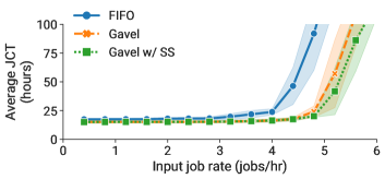
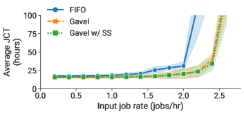
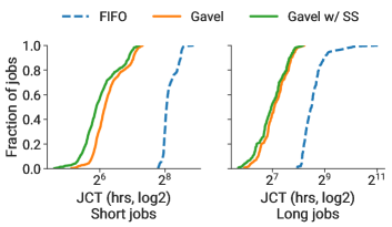
The heterogeneity-aware versions of FIFO allow the cluster to support higher load (in terms of average input job rate). At high load, the heterogeneity-aware version without space sharing reduces average JCT by up to 2.7$\times$, and the heterogeneity-aware version with space sharing reduces average JCT by up to 3.8$\times$. Space sharing is less effective for distributed jobs: it reduces average JCT by 1.1$\times$ for the trace with distributed jobs, and by 1.4$\times$ for the single-GPU trace.

LAS with priorities.

We also run an experiment with the LAS policies where 20% of jobs have higher priority. At high load, Gavel reduces the average JCT of high-priority jobs by 1.5$\times$ and the average JCT of low-priority jobs by 2.7$\times$.

(a) Fraction of total throughput for each job with time.

(b) Total throughput vs. time.

Figure 11: Behavior of a multi-level fairness policy with time as jobs are added to a small cluster with 3 V100 GPUs, 3 P100 GPUs, and 3 K80 GPUs. Each line represents a separate job, and jobs are added every 4 timesteps. The first 6 jobs belong to entity 0 (weight of entity, $w_{0}=1$), the next 6 jobs belong to entity 1 ($w_{1}=2$), and the last 6 jobs belong to entity 2 ($w_{2}=3$).

Cost.

We simulate each of the cost policies on a 500-job workload comprised of ResNet-50 and A3C jobs. As we observe in Figure 1(b), the ResNet-50 job has the best cost-normalized throughput on the V100 while the A3C job has the best cost-normalized throughput on the K80. Each job’s duration is chosen from $\{0.5,1,2,4,8\}$ days, and each job’s SLO is chosen from $\{1.2\times,2\times,10\times\}$ its duration.

The policy that minimizes cost reduces the total cost compared to the policy that maximizes throughput by a factor of roughly 1.4$\times$. However, approximately 35% of jobs violate their SLO as this policy prioritizes cheaper but slower GPUs; in particular, the A3C jobs are scheduled on K80 GPUs which results in violations for tight SLOs. In comparison, the policy that includes SLOs as well eliminates all violations for a small increase in cost (a cost reduction of 1.23$\times$ compared to the baseline policy), by ensuring that A3C jobs with tight SLOs are run on instances with V100 GPUs.

Multi-level Hierarchical Policies.

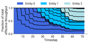
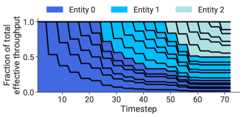
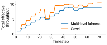
Figure 11 shows the behavior of a multi-level fairness policy as new jobs belonging to multiple entities are added to the cluster. Resources are granted to jobs in a way that respects both the higher-level and lower-level policies: in Figure 11(a), fairness is enforced both within and across entities (as can be seen by the widths of the colored bands, which represents cross-entity fairness, and the widths of bands within a color, which represents fairness across jobs within an entity), and allocations are adjusted as new jobs come in. The Figure 21 in the Appendix shows a similar timeline diagram for a fairness+FIFO policy.

The multi-level fairness policy can also be implemented in a heterogeneity-agnostic manner by statically partitioning resources across users while respecting per-entity and per-user weights. While this results in a fair allocation as well, we observe that total effective throughput is about 17% lower compared to the heterogeneity-aware policy (Figure 11(b)).

7.4 Scalability of Gavel

(a) LAS.

(b) Hierarchical.

Figure 12: Scaling of LAS and hierarchical policies with the number of active jobs on a heterogeneous cluster with an equal number of V100, P100, and K80 GPUs. The size of the cluster is increased as the number of active jobs is increased.

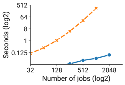
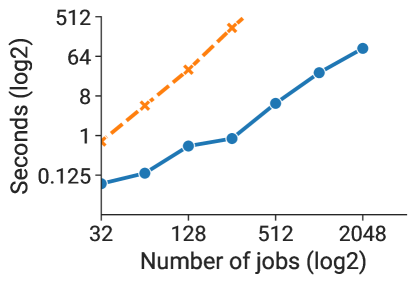
Figure 12 shows the scaling behavior of the heterogeneity-aware LAS and multi-level fairness policies with and without space sharing. We observe that even with 2048 active jobs, the hierarchical policy without space sharing can be run in $<10$ minutes. With space sharing, the policy can be run with 512 jobs in $<10$ minutes. The single-level LAS policy is much cheaper to compute in comparison. We note that allocations do not need to be recomputed every scheduling round – however, the longer the policy takes to run, the longer it takes for a new job to be granted resources on the cluster. Having said that, we believe latencies of $<30$ minutes are acceptable for large clusters (and preferable to a non-preemptive scheduler where jobs might experience large queuing delays).

7.5 Efficacy of Scheduling Mechanism

(a) Effect of round length.

(b) Mechanism vs. ideal.

Figure 13: (a) Effect of round length on average JCT for the heterogeneity-aware LAS policy. (b) Comparison of scheduling mechanism to an ideal baseline that allocates resources to jobs exactly according to the computed allocation for the same policy.

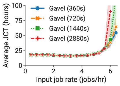
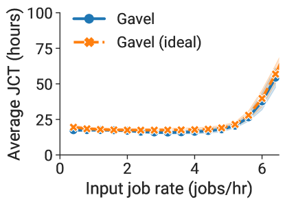
Figure 13(a) shows the effect of the round length on average JCT for the heterogeneity-aware LAS policy with a single-GPU trace. We observed similar behavior on traces with multi-GPU jobs, as well as other policies. A smaller round length gives Gavel’s scheduling mechanism more rounds to course correct, allowing the true allocation and computed optimal allocation to more closely match. We found that the time needed to load and save checkpoints for our target models is $<5$ seconds, which means that a round length of 6 minutes gives a good theoretical tradeoff between fidelity with the optimal allocation and preemption overhead. In practice, hiding this preemption overhead is achievable with careful engineering.

We compare this to an ideal baseline that allocates resources to jobs exactly according to their computed allocation. As shown in Figure 13(b), Gavel’s scheduling mechanism with a round duration of 6 minutes behaves almost identically to this ideal baseline with a single-GPU trace (behavior with a multi-GPU trace is similar).

Figure 14: Comparison of SS-aware LAS policy with estimated throughputs, compared to the SS-aware with oracle throughputs and LAS without space sharing on a heterogeneous 12-GPU cluster.

7.6 Impact of Throughput Estimation

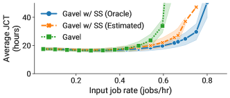
Figure 14 shows the effect of Gavel’s throughput estimator on average JCT when using the space sharing-aware LAS policy compared to the LAS policy without space sharing, and the LAS policy with space sharing and oracle throughputs. The throughput estimator is able to determine missing throughputs in an online fashion accurately enough to observe a very small decrease in average JCT at high load (orange and blue lines).

8 Related Work

Existing DNN Training Schedulers.

Several recent papers have proposed schedulers targeting DNN training workloads.

Gandiva [60] uses time and space sharing to reduce queuing delay and improve resource utilization, but does not specify an explicit scheduling policy. It uses a profiling-based methodology to determine whether to co-locate jobs on an accelerator. However, it does not incorporate model performance data (isolated or co-located performance) into its scheduling policy, resorting to random exploration of job combinations until a combination that improves performance is found, and does not support configurable objectives.

Tiresias [30] and Themis [42] use different objectives to achieve multi-job fairness. However, both do not incorporate jobs’ affinities for different accelerator types in their scheduling objectives, and have scheduling mechanisms strongly coupled with the target policy, making it hard to support other more sophisticated policies like multi-level fairness.

AlloX [39] and $\text{Gandiva}_{\text{fair}}$ [19] are recent DNN schedulers that do consider worker and model heterogeneity. However, both only work for single policies (average job completion time for AlloX, max-min fairness for $\text{Gandiva}_{\text{fair}}$). Moreover, $\text{Gandiva}_{\text{fair}}$ uses a second-price auction mechanism to improve the performance of a heterogeneity-agnostic max-min fairness scheme, but does not provide guarantees as to the optimality of the final allocation. On the other hand, Gavel formalizes each policy as an optimization problem, and can provide a guarantee that the returned solution is “optimal”. Gavel is also able to support more sophisticated policies such as multi-level fairness.

Traditional Cluster Schedulers.

Traditional schedulers such as Mesos [34], Borg [59], TetriSched [56], and YARN [58] support workloads with fixed heterogeneous resource requests, but do not reason about the diverse performance characteristics of jobs across accelerators. Mesos and YARN do not reason about interchangeable resource types that can run the same computation: for example, Mesos’s DRF multi-resource sharing policy [28] decides how to give jobs allocations of distinct resource types, such as RAM and CPUs, but assumes that each job has declared which resources it needs to use and in what ratio (unlike our case, where accelerators display heterogeneous performance behavior).

The multi-interchangeable resource allocation (MIRA) problem [55] also introduces the notion of effective throughput similar to Gavel, but does not demonstrate how this can be used to specify policies as optimization problems, does not consider performance optimizations like space sharing and placement sensitivity, and does not discuss how computed allocations can be realized on physical resources.

Omega [52], Apollo [17], and Hydra [22] are schedulers that take into account the fact that the target workload shows heterogeneity in the number and duration of constituent tasks. However, tasks largely take the same time on different CPUs, and heterogeneity in memory capacities only impacts the number and size of tasks that can be placed on a server. In our work, the compute devices themselves are interchangeable with sometimes large performance differences, and policies decide the time fractions of resources each job should receive while optimizing for various end objectives.

Dynamic Performance Estimation.

As detailed in §6, Gavel uses the approach proposed by Quasar [23] to estimate co-located job performance online. In particular, Gavel uses a mix of profiling and matrix completion to compute a “fingerprint” against a set of reference models profiled offline. In this work, we show that the techniques used by Quasar can be successfully applied to this new setting.

9 Conclusion

In this paper, we proposed Gavel, a heterogeneity-aware cluster scheduler that is able to optimize for many high-level metrics like fairness, makespan, and cost. Gavel demonstrates how existing policies can be expressed as optimization problems, and extends these policies to be heterogeneity-aware. Gavel then uses a decoupled round-based scheduling mechanism to ensure that the computed optimal allocation is realized. Gavel’s heterogeneity-aware policies improve end objectives both on a physical and simulated cluster. It can support a higher maximum cluster load, while improving objectives such as average job completion time by 3.5$\times$, makespan by 2.5$\times$, and cost by 1.4$\times$.

Appendix A Appendix

In this section, we describe how more complicated optimization problem formulations can be solved in practice, and present additional results.

A.1 Policies requiring multi-step solutions

Minimize makespan.

The makespan policy tries to allocate resources to jobs in such a way that all active jobs are completed as soon as possible. To compute an allocation for this policy, we can binary search for the smallest makespan $M$ that satisfies the following constraints,

$$\text{num\_steps}_{m}\leq\text{throughput}(m,X)\cdot M \forall m$$

$$0\leq X_{mj}\leq 1 \forall(m,j)$$

$$\sum_{j}X_{mj}\leq 1 \forall m$$

$$\sum_{m}X_{mj}\leq 1 \forall j$$

Identifying bottleneck jobs in fairness policy.

Solving a max-min fairness policy, such as LAS or hierarchical fairness, results in an allocation that satisfies fairness metrics but may underutilize resources in scenarios where the bottlenecked job’s throughput is matched by other jobs without using all available resources. Identifying bottleneck jobs after an iteration of a fairness policy computation can be done by solving a mixed-integer linear program. The binary integer variable $z_{m}$ is set to 1 when job $m$’s scaled effective throughput can be improved without causing any other job’s scaled effective throughput to drop below the minimum computed in the previous iteration of the policy’s LP. We identify all jobs which are stuck as $\{m:z_{m}=0\}$ by computing an allocation that maximizes the sum of all $z_{m}$:

$$\text{Maximize}_{X}\sum_{\{m:p_{m}>0\}}z_{m}$$

subject to:

$$z_{m}=\begin{cases}1&\text{ if }\text{throughput}(m,X)>\text{throughput}(m,X^{\text{prev}})\\ 0&\text{otherwise}\end{cases}$$

The conditional constraint on $z_{m}$ can be expressed as two linear inequalities:

$$\text{throughput}(m,X^{\text{prev}})<\text{throughput}(m,X)+Y(1-z_{m})$$

$$\text{throughput}(m,X^{\text{prev}})\geq\text{throughput}(m,X)-Yz_{m}$$

where $Y$ is a sufficiently large number such that it is not an active constraint, such as the max throughput of the job.

A.2 Additional Results

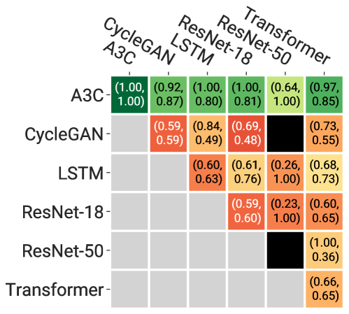
Figure 15 shows the performance of colocated DNN models on a single NVIDIA P100 GPU, presented as a heat map.

Figures 16, 17, 18, 19, and 20 show a comparison of vanilla, heterogeneity-agnostic policies with their heterogeneity-aware counterparts on single-worker and multi-worker traces. We see across the board that Gavel’s heterogeneity-aware policies allow the cluster to support higher load (in terms of average job input rate), and also reduce end objectives.

Figure 21 shows the behavior of a multi-level fairness policy that combines a higher-level fairness policy with a low-level FIFO policy. The widths of the colored bands are in the ratios of the weights of each entity; within an entity, the effective throughputs of jobs are ordered in a way that respects the arrival order of jobs within that entity. All jobs within low-weight entities do not receive resources under high load.

Figure 15: Performance of several DNN models when run concurrently on a single P100 GPU. The cell at row $i$ and column $j$ reports the normalized throughput (iterations/second) achieved by co-located models $i$ and $j$. Throughputs are normalized with respect to the throughput achieved by each model when run in isolation. Black squares show jobs that cannot co-locate due to memory constraints.

(a) Average job completion time vs. cluster load.

(b) CDF of job completion times.

Figure 16: Comparison of heterogeneity-agnostic FIFO policy to a heterogeneity-aware FIFO policy, on the simulated cluster and continuous-single trace.

(a) Average job completion time vs. cluster load.

(b) CDF of job completion times.

Figure 17: Comparison of heterogeneity-agnostic finish time fairness (FTF) policy to a heterogeneity-aware FTF policy, on the simulated cluster and continuous-single trace.

(a) Average job completion time vs. cluster load.

(b) CDF of job completion times.

Figure 18: Comparison of heterogeneity-agnostic FIFO policy to a heterogeneity-aware FIFO policy, on the simulated cluster and continuous-multiple trace.

Figure 19: Comparison of heterogeneity-agnostic makespan policy to a heterogeneity-aware makespan policy, as well as FIFO and Gandiva baselines on the simulated cluster and the static-multiple trace.

Figure 20: Comparison of heterogeneity-agnostic LAS policy to a heterogeneity-aware LAS policy, on the simulated cluster, continuous-multiple trace, with 20% of jobs with high priority.

Figure 21: Timeline showing behavior of a hierarchical policy (fairness as top-level policy, FIFO as bottom-level policy) with time. A job is added every 4 timesteps. The first 6 jobs belong to entity 0, the next 6 jobs belong to entity 1, and the last 6 jobs belong to entity 2. Entity 0 has a weight of 1, entity 1 has a weight of 2, and entity 2 has a weight of 3. Real throughputs are used, and jobs are sampled from those shown in Table 2.

References

- [1] AWS Accelerator Offerings. https://aws.amazon.com/ec2/instance-types/, 2020.
- [2] Cloud GPUs on GCP. https://cloud.google.com/gpu, 2020.
- [3] Cloud TPUs on GCP. https://cloud.google.com/tpu, 2020.
- [4] ElasticDL. https://github.com/sql-machine-learning/elasticdl, 2020.
- [5] gRPC. https://grpc.io, 2020.
- [6] ImageNet Training in PyTorch. https://github.com/pytorch/examples/tree/master/imagenet, 2020.
- [7] Implementing Core Scheduler Functionality in Resource Manager (V1) for Hadoop. https://issues.apache.org/jira/browse/HADOOP-3445, 2020.
- [8] Job Scheduling in Spark. https://spark.apache.org/docs/latest/job-scheduling.html#scheduling-within-an-application, 2020.
- [9] Linear-fractional Optimization. http://www.seas.ucla.edu/~vandenbe/ee236a/lectures/lfp.pdf, 2020.
- [10] Microsoft Philly Trace. https://github.com/msr-fiddle/philly-traces, 2020.
- [11] NVIDIA Multi-Process Service. https://docs.nvidia.com/deploy/pdf/CUDA_Multi_Process_Service_Overview.pdf, 2020.
- [12] Word-level Language Modeling RNN. https://github.com/pytorch/examples/tree/master/word_language_model, 2020.
- [13] YARN – The Capacity Scheduler. https://blog.cloudera.com/yarn-capacity-scheduler/, 2020.
- [14] M. Abadi, P. Barham, J. Chen, Z. Chen, A. Davis, J. Dean, M. Devin, S. Ghemawat, G. Irving, M. Isard, et al. TensorFlow: A System for Large-Scale Machine Learning. In 12th USENIX Symposium on Operating Systems Design and Implementation (OSDI 16), pages 265–283, 2016.
- [15] D. Amodei, S. Ananthanarayanan, R. Anubhai, J. Bai, E. Battenberg, C. Case, J. Casper, B. Catanzaro, Q. Cheng, G. Chen, et al. Deep Speech 2: End-to-End Speech Recognition in English and Mandarin. In International Conference on Machine Learning, pages 173–182, 2016.
- [16] D. P. Bertsekas and R. G. Gallager. Data Networks. 1987.
- [17] E. Boutin, J. Ekanayake, W. Lin, B. Shi, J. Zhou, Z. Qian, M. Wu, and L. Zhou. Apollo: Scalable and Coordinated Scheduling for Cloud-Scale Computing. In 11th USENIX Symposium on Operating Systems Design and Implementation (OSDI 14), pages 285–300, 2014.
- [18] E. J. Candes and Y. Plan. Matrix Completion with Noise. Proceedings of the IEEE, 98(6):925–936, 2010.
- [19] S. Chaudhary, R. Ramjee, M. Sivathanu, N. Kwatra, and S. Viswanatha. Balancing Efficiency and Fairness in Heterogeneous GPU Clusters for Deep Learning. In Proceedings of the Fifteenth European Conference on Computer Systems, pages 1–16, 2020.
- [20] W. Chen, J. Rao, and X. Zhou. Preemptive, Low Latency Datacenter Scheduling via Lightweight Virtualization. In USENIX Annual Technical Conference, USENIX ATC 2017, pages 251–263, 2017.
- [21] C. Coleman, D. Kang, D. Narayanan, L. Nardi, T. Zhao, J. Zhang, P. Bailis, K. Olukotun, C. Ré, and M. Zaharia. Analysis of DAWNBench, A Time-to-Accuracy Machine Learning Performance Benchmark. ACM SIGOPS Operating Systems Review, 53(1):14–25, 2019.
- [22] C. Curino, S. Krishnan, K. Karanasos, S. Rao, G. M. Fumarola, B. Huang, K. Chaliparambil, A. Suresh, Y. Chen, S. Heddaya, et al. Hydra: A Federated Resource Manager for Data-Center Scale Analytics. In 16th USENIX Symposium on Networked Systems Design and Implementation (NSDI 19), pages 177–192, 2019.
- [23] C. Delimitrou and C. Kozyrakis. Quasar: Resource-Efficient and QoS-Aware Cluster Management. In ACM SIGARCH Computer Architecture News, volume 42, pages 127–144, 2014.
- [24] J. Deng, W. Dong, R. Socher, L.-J. Li, K. Li, and L. Fei-Fei. ImageNet: A Large-Scale Hierarchical Image Database. In Proceedings of the IEEE Conference on Computer Vision and Pattern Recognition, pages 248–255, 2009.
- [25] S. Diamond and S. Boyd. CVXPY: A Python-Embedded Modeling Language for Convex Optimization. The Journal of Machine Learning Research, 17(1):2909–2913, 2016.
- [26] D. Elliott, S. Frank, K. Sima’an, and L. Specia. Multi30K: Multilingual English-German Image Descriptions. In Proceedings of the 5th Workshop on Vision and Language, pages 70–74. Association for Computational Linguistics, 2016.
- [27] J. Fowers, K. Ovtcharov, M. Papamichael, T. Massengill, M. Liu, D. Lo, S. Alkalay, M. Haselman, L. Adams, M. Ghandi, et al. A Configurable Cloud-Scale DNN Processor for Real-Time AI. In 2018 ACM/IEEE 45th Annual International Symposium on Computer Architecture (ISCA), pages 1–14, 2018.
- [28] A. Ghodsi, M. Zaharia, B. Hindman, A. Konwinski, S. Shenker, and I. Stoica. Dominant Resource Fairness: Fair Allocation of Multiple Resource Types. In 8th USENIX Symposium on Networked Systems Design and Implementation (NSDI 11), pages 24–24, 2011.
- [29] D. Griffis. RL A3C PyTorch. https://github.com/dgriff777/rl_a3c_pytorch, 2020.
- [30] J. Gu, M. Chowdhury, K. G. Shin, Y. Zhu, M. Jeon, J. Qian, H. Liu, and C. Guo. Tiresias: A GPU Cluster Manager for Distributed Deep Learning. In 16th USENIX Symposium on Networked Systems Design and Implementation (NSDI 19), pages 485–500, 2019.
- [31] F. M. Harper and J. A. Konstan. The MovieLens Datasets: History and Context. ACM Transactions on Interactive Intelligent Systems (TIIS), 5(4):19, 2016.
- [32] K. He, G. Gkioxari, P. Dollár, and R. Girshick. Mask R-CNN. In Proceedings of the IEEE International Conference on Computer Vision, pages 2961–2969, 2017.
- [33] K. He, X. Zhang, S. Ren, and J. Sun. Deep Residual Learning for Image Recognition. In Proceedings of the IEEE Conference on Computer Vision and Pattern Recognition, pages 770–778, 2016.
- [34] B. Hindman, A. Konwinski, M. Zaharia, A. Ghodsi, A. D. Joseph, R. H. Katz, S. Shenker, and I. Stoica. Mesos: A Platform for Fine-Grained Resource Sharing in the Data Center. In 8th USENIX Symposium on Networked Systems Design and Implementation (NSDI 11), pages 22–22, 2011.
- [35] Y.-H. Huang. Attention is All You Need: A PyTorch Implementation. https://github.com/jadore801120/attention-is-all-you-need-pytorch, 2018.
- [36] M. Jeon, S. Venkataraman, A. Phanishayee, J. Qian, W. Xiao, and F. Yang. Analysis of Large-Scale Multi-Tenant GPU Clusters for DNN Training Workloads. In USENIX Annual Technical Conference, USENIX ATC 2019, pages 947–960, 2019.
- [37] N. P. Jouppi, C. Young, N. Patil, D. Patterson, G. Agrawal, R. Bajwa, S. Bates, S. Bhatia, N. Boden, A. Borchers, et al. In-Datacenter Performance Analysis of a Tensor Processing Unit. In 2017 ACM/IEEE 44th Annual International Symposium on Computer Architecture (ISCA), pages 1–12, 2017.
- [38] A. Krizhevsky, V. Nair, and G. Hinton. The CIFAR-10 Dataset. online: http://www. cs. toronto. edu/kriz/cifar. html, 55, 2014.
- [39] T. N. Le, X. Sun, M. Chowdhury, and Z. Liu. AlloX: Compute Allocation in Hybrid Clusters. In Proceedings of the Fifteenth European Conference on Computer Systems, pages 1–16, 2020.
- [40] E. Linder-Norén. PyTorch-GAN. https://github.com/eriklindernoren/PyTorch-GAN#cyclegan, 2020.
- [41] K. Liu. Train CIFAR-10 with PyTorch. https://github.com/kuangliu/pytorch-cifar, 2020.
- [42] K. Mahajan, A. Balasubramanian, A. Singhvi, S. Venkataraman, A. Akella, A. Phanishayee, and S. Chawla. Themis: Fair and Efficient GPU Cluster Scheduling. In 17th USENIX Symposium on Networked Systems Design and Implementation (NSDI 20), pages 289–304, 2020.
- [43] H. Mao, M. Schwarzkopf, S. B. Venkatakrishnan, Z. Meng, and M. Alizadeh. Learning Scheduling Algorithms for Data Processing Clusters. In Proceedings of the ACM Special Interest Group on Data Communication, pages 270–288. 2019.
- [44] S. Merity, C. Xiong, J. Bradbury, and R. Socher. Pointer Sentinel Mixture Models. In 5th International Conference on Learning Representations, ICLR 2017, Toulon, France, April 24-26, 2017, Conference Track Proceedings, 2017.
- [45] A. Mnih and R. R. Salakhutdinov. Probabilistic Matrix Factorization. In Advances in Neural Information Processing Systems, pages 1257–1264, 2008.
- [46] V. Mnih, A. P. Badia, M. Mirza, A. Graves, T. Lillicrap, T. Harley, D. Silver, and K. Kavukcuoglu. Asynchronous Methods for Deep Reinforcement Learning. In International Conference on Machine Learning, pages 1928–1937, 2016.
- [47] A. Moussawi. Towards Large Scale Training of Autoencoders for Collaborative Filtering. In Proceedings of Late-Breaking Results Track Part of the Twelfth ACM Conference on Recommender Systems, RecSys’18, Vancouver, BC, Canada, 2018.
- [48] D. Narayanan, A. Harlap, A. Phanishayee, V. Seshadri, N. R. Devanur, G. R. Ganger, P. B. Gibbons, and M. Zaharia. PipeDream: Generalized Pipeline Parallelism for DNN Training. In Proceedings of the 27th ACM Symposium on Operating Systems Principles, pages 1–15, 2019.
- [49] D. Narayanan, K. Santhanam, A. Phanishayee, and M. Zaharia. Accelerating Deep Learning Workloads through Efficient Multi-Model Execution. In NeurIPS Workshop on Systems for Machine Learning (December 2018), 2018.
- [50] A. Paszke, S. Gross, F. Massa, A. Lerer, J. Bradbury, G. Chanan, T. Killeen, Z. Lin, N. Gimelshein, L. Antiga, et al. PyTorch: An Imperative Style, High-Performance Deep Learning Library. In Advances in Neural Information Processing Systems, pages 8024–8035, 2019.
- [51] B. Radunovic and J.-Y. Le Boudec. A Unified Framework for Max-Min and Min-Max Fairness with Applications. IEEE/ACM Transactions on Networking, 15(5):1073–1083, 2007.
- [52] M. Schwarzkopf, A. Konwinski, M. Abd-El-Malek, and J. Wilkes. Omega: Flexible, Scalable Schedulers for Large Compute Clusters. In Proceedings of the 8th ACM European Conference on Computer Systems, pages 351–364, 2013.
- [53] M. J. Shafiee, B. Chywl, F. Li, and A. Wong. Fast YOLO: A Fast You Only Look Once System for Real-Time Embedded Object Detection in Video. arXiv preprint arXiv:1709.05943, 2017.
- [54] P. Sinha and A. A. Zoltners. The Multiple-Choice Knapsack Problem. Operations Research, 27(3):503–515, 1979.
- [55] X. Sun, T. N. Le, M. Chowdhury, and Z. Liu. Fair Allocation of Heterogeneous and Interchangeable Resources. ACM SIGMETRICS Performance Evaluation Review, 46(2):21–23, 2019.
- [56] A. Tumanov, T. Zhu, J. W. Park, M. A. Kozuch, M. Harchol-Balter, and G. R. Ganger. Tetrisched: Global Rescheduling with Adaptive Plan-Ahead in Dynamic Heterogeneous Clusters. In Proceedings of the Eleventh European Conference on Computer Systems, page 35. ACM, 2016.
- [57] A. Vaswani, N. Shazeer, N. Parmar, J. Uszkoreit, L. Jones, A. N. Gomez, Ł. Kaiser, and I. Polosukhin. Attention is All You Need. In Advances in Neural Information Processing Systems, pages 5998–6008, 2017.
- [58] V. K. Vavilapalli, A. C. Murthy, C. Douglas, S. Agarwal, M. Konar, R. Evans, T. Graves, J. Lowe, H. Shah, S. Seth, et al. Apache Hadoop YARN: Yet Another Resource Negotiator. In Proceedings of the 4th Annual Symposium on Cloud Computing, page 5. ACM, 2013.
- [59] A. Verma, L. Pedrosa, M. Korupolu, D. Oppenheimer, E. Tune, and J. Wilkes. Large-scale Cluster Management at Google with Borg. In Proceedings of the Tenth European Conference on Computer Systems, page 18, 2015.
- [60] W. Xiao, R. Bhardwaj, R. Ramjee, M. Sivathanu, N. Kwatra, Z. Han, P. Patel, X. Peng, H. Zhao, Q. Zhang, et al. Gandiva: Introspective Cluster Scheduling for Deep Learning. In 13th USENIX Symposium on Operating Systems Design and Implementation (OSDI 18), pages 595–610, 2018.
- [61] M. Zaharia, D. Borthakur, J. Sen Sarma, K. Elmeleegy, S. Shenker, and I. Stoica. Delay Scheduling: A Simple Technique for Achieving Locality and Fairness in Cluster Scheduling. In Proceedings of the 5th European Conference on Computer Systems, pages 265–278. ACM, 2010.
- [62] J.-Y. Zhu, T. Park, P. Isola, and A. A. Efros. Unpaired Image-to-Image Translation using Cycle-Consistent Adversarial Networks. In Proceedings of the IEEE International Conference on Computer Vision, pages 2223–2232, 2017.