Nuclear quantum effects in graphane

Abstract

Graphane is a quasi-two-dimensional material consisting of a single layer of fully hydrogenated graphene, with a C:H ratio of 1. We study nuclear quantum effects in the so-called chair-graphane by using path-integral molecular dynamics (PIMD) simulations. The interatomic interactions are modeled by a tight-binding potential model fitted to density-functional calculations. Finite-temperature properties are studied in the range from 50 to 1500 K. To assess the magnitude of nuclear quantum effects in the properties of graphane, classical molecular dynamics simulations have been also performed. These quantum effects are significant in structural properties such as interatomic distances and layer area at finite temperatures. The in-plane compressibility of graphane is found to be about twice larger than that of graphene, and at low temperature it is 9% higher than the classical calculation. The thermal expansion coefficient resulting from PIMD simulations vanishes in the zero-temperature limit, in agreement with the third law of Thermodynamics.

I Introduction

Carbon-based materials have been intensively investigated in recent years, in particular those consisting of two-dimensional (2D) layers Geim and Novoselov (2007); Woods et al. (2014); Meunier et al. (2016); Castro Neto et al. (2009); Cao et al. (2018); Yankowitz et al. (2019). In this context, hydrogenated graphene (called graphane) is a quasi-2D structure of C atoms ordered in a buckled honeycomb lattice covalently bonded to H atoms. The most studied conformer of graphane is the so-called chair-graphane, where H atoms alternate in a chairlike arrangement on both sides of the carbon layer Sofo et al. (2007); Wen et al. (2011). This graphane configuration is studied in this paper. There exist also boat- and washboard-graphane Cadelano et al. (2010), which will not be considered here.

Graphane can be reversibly obtained by hydrogen chemisorption on pure graphene Elias et al. (2009), which causes a rearrangement of the chemical bonds and angles in the honeycomb lattice of graphene. Each C atom is bound to an H neighbor, changing its orbital hybridization from sp² to sp³, and the planar configuration of graphene is modified into an out-of-plane buckled structure. Graphane is a wide band-gap semiconductor, where appreciable spin polarization can be achieved by the creation of domains of H vacancies and CH divacancies Sahin et al. (2010). Moreover, the presence of impurities such as Li atoms or metal dopants may significantly affect its electronic and magnetic properties Wang et al. (2016a); Mapasha et al. (2017); Eng et al. (2013).

A deep comprehension of structural and thermal properties of 2D systems is a challenging problem in modern statistical physics Safran (1994); Nelson et al. (2004); Tarazona et al. (2013), which has been mainly discussed in the field of biological membranes and soft condensed matter Fournier and Barbetta (2008); Tarazona et al. (2013). However, the large complexity of these systems makes it difficult to devise microscopic models on the basis of realistic interatomic interactions. 2D carbon-based materials provide us with model systems where atomic-scale studies are possible, allowing for a deeper understanding of the physical properties of this type of systems Pop et al. (2012); Fong et al. (2013); Wang et al. (2016b); Herrero and Ramírez (2018a).

At finite temperatures, thermally excited ripples appear and distort the lattice of 2D materials. It has been suggested that in graphane the aspect of these ripples may be different from those in graphene. This could be a consequence of the fact that in graphane the thermal energy can be accommodated on the in-plane bending modes (involving C-C-C bond angles in the buckled configuration), instead of leading to significant out-of-plane fluctuations, as happens in graphene Costamagna et al. (2012); Gao and Huang (2014).

In several electronic-structure calculations of graphane presented in the literature, even though they are based on precise ab-initio quantum mechanical methods, atomic nuclei are described as classical particles Sofo et al. (2007); Cadelano et al. (2010); Leenaerts et al. (2010); Zhou et al. (2013); Chechin et al. (2014), so that some quantum effects such as zero-point motion are not included in the calculation. Finite-temperature properties of graphane have been also studied by molecular dynamics simulations using ab-initio Chechin et al. (2014) and empirical interatomic potentials Costamagna et al. (2012); Liu et al. (2013). In these simulations, atomic nuclei were also treated as classical particles.

Nuclear quantum effects may be important for vibrational and electronic properties of relatively light elements like carbon, and even more for hydrogen, especially at low temperatures. To take into account the quantum nature of the nuclei, path-integral (Monte Carlo and molecular dynamics) simulations are especially adequate, since the nuclear degrees of freedom can be efficiently quantized, allowing one to study quantum and thermal fluctuations at finite temperatures Gillan (1988); Ceperley (1995). This procedure permits to perform quantitative studies of anharmonic effects in condensed matter Herrero and Ramírez (1995); Ramírez and Herrero (2011).

In this paper we use the path-integral molecular dynamics (PIMD) method to study the influence of nuclear quantum dynamics on structural, vibrational, and thermal properties of graphane at temperatures from 50 to 1500 K. The interatomic interactions are described by an efficient tight-binding (TB) Hamiltonian, developed on the basis of density-functional calculations. We consider simulation cells of different sizes, as finite-size effects can be relevant for some variables, such as the atomic delocalization in the out-of-plane direction Gao and Huang (2014); Los et al. (2016). Path-integral methods similar to that employed here have been applied before to study nuclear quantum effects in carbon-based materials as diamond Herrero and Ramírez (2000); Ramírez et al. (2006); Herrero and Ramírez (2007), and more recently in graphene Brito et al. (2015); Hasik et al. (2018); Herrero and Ramírez (2016). The adsorption and diffusion of H on graphene has been also studied by using this kind of techniques Davidson et al. (2014); Herrero and Ramírez (2009). Moreover, nuclear quantum effects have been analyzed earlier by using a combination of density-functional theory and a quasi-harmonic approximation for vibrational modes in graphane Huang and Zeng (2013).

The paper is organized as follows. In Sec. II we describe the computational techniques employed here: PIMD method, tight-binding procedure, and calculation of atomic mean-square displacements. In Sec. III we present results for the internal energy of graphane, with emphasis on its constituent parts, i.e., kinetic and potential energy. Results for structural properties are given in Sec.  IV (interatomic distances) and Sec.  V (orientation of the C–H bonds). In Sec. VI we study the atomic motion, as visualized from mean-square displacements in the in-plane and out-of-plane directions. Data for the layer area and the in-plane compressibility of graphane are given in Secs.  VII and VIII, respectively. The paper closes in Sec. IX with a summary of the main results.

II Computational Method

II.1 Path-integral molecular dynamics

We use the PIMD method to obtain equilibrium properties of graphane at several temperatures. This procedure, based on the Feynman path-integral formulation of statistical mechanics Feynman (1972), is a nonperturbative approach suitable to study finite-temperature properties of many-body quantum systems. It profits from the fact that the partition function of a quantum system may be expressed in a way formally equivalent to that of a classical one, obtained by replacing each quantum particle by a ring polymer formed by $N_{\rm Tr}$ (Trotter number) classical particles, linked by harmonic springs Feynman (1972); Kleinert (1990); Ceperley (1995). Details on this simulation technique can be found elsewhere Chandler and Wolynes (1981); Gillan (1988); Tuckerman (2010); Herrero and Ramírez (2014).

We employ the molecular dynamics method to sample the configuration space of the classical isomorph of our quantum system. The dynamics in this computational procedure is artificial, since it does not represent the actual quantum dynamics of the real particles. Nevertheless, it is well-suited for effectively sampling the many-body configuration space, yielding accurate values for time-independent equilibrium properties of the quantum system under consideration. The calculations presented here were performed in the isothermal-isobaric ensemble, where we fix the number of atoms ($N$ pairs C–H), the in-plane applied stress (here $\tau=0$), and the temperature ($T$). The stress $\tau$ in the $(x,y)$ plane, with units of force per unit length, coincides with the so-called mechanical or frame tension Ramírez and Herrero (2017); Fournier and Barbetta (2008); Shiba et al. (2016); Herrero and Ramírez (2018b). We have used effective algorithms for carrying out the PIMD simulations in the $N\tau T$ ensemble, as those presented in the literature Martyna et al. (1999); Tuckerman (2010). Specifically, staging variables have been employed to define the bead coordinates, and the constant-temperature ensemble was achieved by coupling chains of four Nosé-Hoover thermostats to each staging variable. Moreover, a chain of four barostats was coupled to the in-plane area of the simulation cell to give the required pressure, $\tau=0$ Tuckerman (2010); Herrero and Ramírez (2014).

Figure 1: RMS fluctuations of the kinetic and potential energy for graphane vs the temperature, as derived from PIMD simulations. Circles: potential energy; squares: kinetic energy of hydrogen; diamonds: kinetic energy of carbon. Error bars are smaller than the symbol size. Lines are guides to the eye.

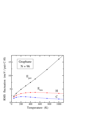
The equations of motion have been integrated by using the reversible reference system propagator algorithm (RESPA), which permits us to define different time steps for the integration of the slow and fast degrees of freedom Martyna et al. (1996). The time step employed for the dynamics related to interatomic forces was $\Delta t$ = 0.5 fs, which turned out to be suitable for the atomic masses and temperatures considered here, and provided good convergence for the studied variables. For the evolution of the fast dynamical variables, including thermostats and harmonic bead interactions, we employed a time step $\delta t=\Delta t/4$, as in previous simulations Herrero et al. (2006). The kinetic energy, $E_{\rm kin}$, has been calculated by means of the so-called virial estimator, which has a statistical uncertainty smaller than the potential energy of the system, especially at high temperatures Herman et al. (1982); Tuckerman (2010). This can be seen in Fig. 1, where we have plotted the root mean-square (RMS) fluctuations of the kinetic ($E_{\rm kin}$) and potential ($E_{\rm pot}$) energy as a function of temperature. The RMS fluctuations of $E_{\rm pot}$ increase for rising $T$, while those of $E_{\rm kin}$ reach a maximum and then decrease at high $T$ for both H and C.

The configuration space of graphane for simulation cells including $2N$ atoms ($N$ pairs C–H, with $N$ from 24 to 216), has been sampled at temperatures between 50 and 1500 K. For the smallest size, $N$ = 24, PIMD simulations at $T$ = 25 K were performed. To compare with the results of our quantum simulations, some classical molecular dynamics (MD) simulations of graphane have been also carried out. In our context, this is achieved by setting the Trotter number $N_{\rm Tr}$ = 1. In the quantum simulations, $N_{\rm Tr}$ was taken proportional to the inverse temperature, so that $N_{\rm Tr}\,T$ = 6000 K. This choice keeps roughly constant the precision associated to the finite values of $N_{\rm Tr}$ at different temperatures Herrero et al. (2006).

Figure 2: Snapshot taken from of a simulation of graphane (96 C + 96 H) at $T=300$ K. Large dark and small white circles represent carbon and hydrogen atoms, respectively.

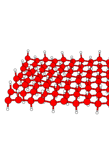
We considered rectangular simulation cells with similar side length in the $x$ and $y$ directions of the $(x,y)$ reference plane ($L_{x}\approx L_{y}$), for which periodic boundary conditions were assumed. In the out-of-plane $z$-direction, we have free boundary conditions, so that C and H atoms can unrestrictedly move, simulating a free-standing graphane layer. For a given temperature, a typical simulation run consisted of $10^{5}$ PIMD steps for system equilibration, followed by $2\times 10^{6}$ steps for the calculation of ensemble average properties, except for the cell size $N=216$, for which the trajectories included $8\times 10^{5}$ steps. In Fig. 2 we present a view of a graphane configuration obtained in our simulations at $T=300$ K. In this picture, red and white circles represent C and H atoms, respectively.

For comparison with our results for graphane, we have performed some PIMD simulations of graphene with the same TB potential as that used for graphane (see below). For graphene, we employed cells consisting of $N$ carbon atoms, with $N$ = 96 and 216. Moreover, some simulations were carried out for a single H impurity on graphene, similar to those presented earlier Herrero and Ramírez (2009). In the present case, however, these simulations were performed in the isothermal-isobaric ensemble, as those of graphane, vs the constant in-plane area simulations in Ref. Herrero and Ramírez (2009).

II.2 Tight-binding procedure

The calculations presented here have been carried out within the adiabatic (Born-Oppenheimer) approximation, which permits to define a potential-energy surface for the nuclear coordinates. A relevant point in the PIMD procedure is a satisfactory description of the interatomic interactions, which should be as realistic as possible. Using density functional or Hartree-Fock based self-consistent potentials requires computational resources that would considerably restrict the size of the manageable simulation cells and/or the number of accessible PIMD steps. Thus, we obtain the Born-Oppenheimer surface for the nuclear dynamics from an efficient tight-binding Hamiltonian, based on density functional calculations Porezag et al. (1995).

The capability of TB methods to accurately describe various properties of molecules and solids was reviewed by Goringe et al. Goringe et al. (1997). We have checked the predictions of this TB potential for well-known frequencies of C–H vibrations in small molecules. For example, for CH₄ it predicts in a harmonic approximation frequencies of 3100 and 3242 cm^-1 for C–H modes with symmetry $A_{1}$ and $T_{2}$, respectively Herrero et al. (2006), to be compared with values of 2917 and 3019 cm^-1 obtained from vibrational spectroscopy Johnson et al. (1993). If one considers the anharmonic shift associated to these modes (usually towards lower frequencies), the accord is acceptable. A detailed study of vibrational frequencies in hydrocarbon molecules obtained with this TB potential, taking into account mode anharmonicities, was presented elsewhere López-Ciudad et al. (2003); Böhm et al. (2001). We have used earlier this TB Hamiltonian to describe carbon-hydrogen interactions in diamond Herrero et al. (2006); Herrero and Ramírez (2007), graphite Herrero and Ramírez (2010), and graphene Herrero and Ramírez (2009).

Figure 3: Convergence of the potential energy of graphane for different cell sizes ($N$). The zero of energy is taken for $N=384$. Note the logarithmic scale in the horizontal axis.

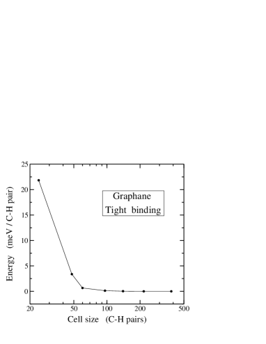
An advantage of the combination of path integrals with electronic structure methods is that both electrons and atomic nuclei are treated quantum mechanically, so that phonon-phonon and electron-phonon interactions are directly taken into account in the simulation. For the reciprocal-space sampling we have employed only the $\Gamma$ point (${\bf k}=0$), as the main effect of using a larger ${\bf k}$ set is a nearly constant shift in the total energy, with little influence in the calculation of energy differences. In Fig. 3 we present the convergence of the potential energy of graphane for different cell sizes $N$. The data points correspond to $E_{\rm pot}$ obtained with the TB model for the minimum-energy configuration (classical, $T=0$).

II.3 Mean-square displacements

An interesting application of PIMD simulations is the study of atomic delocalization in three-dimensional (3D) space at finite temperatures. This includes a thermal (classical) delocalization, and another associated to the quantum nature of atomic nuclei, which may be assessed by the extension of the quantum paths sampled in the simulations. For a path of nucleus $i$ ($i=1,...,2N$), we define the centroid (center of mass) as

$$\overline{\bf r}_{i}=\frac{1}{N_{\rm Tr}}\sum_{j=1}^{N_{\rm Tr}}{\bf r}_{ij}\;,$$ (1)

where ${\bf r}_{ij}\equiv(x_{ij},y_{ij},z_{ij})$ is the position of bead $j$ in the associated ring polymer.

The mean-square displacement $(\Delta x)^{2}_{i}$ of nucleus $i$ in the $x$ direction along a PIMD simulation run is defined as

$$(\Delta x)^{2}_{i}=\frac{1}{N_{\rm Tr}}\sum_{j=1}^{N_{\rm Tr}}\left<(x_{ij}-\left<\overline{x}_{i}\right>)^{2}\right>\,.$$ (2)

In this expression $\overline{x}_{i}$ is the instantaneous $x$-coordinate of the centroid of atom $i$, and $\left<\overline{x}_{i}\right>$ is the average value along a simulation run, which corresponds to the observable $x$-coordinate of the atomic position. Thus, $\left<(x_{ij}-\left<\overline{x}_{i}\right>)^{2}\right>$ is the mean-square displacement (MSD) of the coordinate $x_{ij}$ of bead $j$ with respect to the average centroid $\left<\overline{x}_{i}\right>$ ($j$ = 1, …, $N_{\rm Tr}$). Hence, $(\Delta x)^{2}_{i}$ is an average of these displacements for the beads associated to nucleus $i$, corresponding to the observable MSD of the atomic coordinate.

The spread of the paths associated to an atomic nucleus can be measured by the mean-square radius-of-gyration of the ring polymers, with an $x$ component Gillan (1988, 1990):

$$Q_{x,i}^{2}=\frac{1}{N_{\rm Tr}}\sum_{j=1}^{N_{\rm Tr}}\left<(x_{ij}-\overline{x}_{i})^{2}\right>\,.$$ (3)

Notice the difference between the r.h.s. of Eqs. (2) and (3): in the former one has an average of the centroid position over the whole trajectory, i.e. $\left<\overline{x}_{i}\right>$, while in the latter there appears the instantaneous value $\overline{x}_{i}$ for each configuration.

At finite temperatures ($T>0$ K), the observable spatial delocalization $(\Delta x)^{2}_{i}$ of nucleus $i$ in the $x$ direction contains, along with $Q_{x,i}^{2}$, another term which takes into account classical-like motion of the centroid coordinate $\overline{x}_{i}$:

$$(\Delta x)^{2}_{i}=C_{x,i}^{2}+Q_{x,i}^{2}\,,$$ (4)

where

$$C_{x,i}^{2}=\langle\overline{x}_{i}^{2}\rangle-\langle\overline{x}_{i}\rangle^{2}\,.$$ (5)

$C_{x,i}^{2}$ is the MSD of the centroid of nucleus $i$, and the quantum component $Q_{x,i}^{2}$ is the average MSD of the path (beads in the ring polymer) with respect to the instantaneous centroid. $C_{x,i}^{2}$ is a semiclassical thermal contribution to $(\Delta x)^{2}_{i}$, as at high temperature it converges to the MSD of a classical model, where the quantum paths converge to single points ($Q_{x,i}^{2}\to 0$). In the limit $T\to 0$, $C_{x,i}^{2}$ vanishes and $Q_{x,i}^{2}$ corresponds to zero-point motion of nucleus $i$. For each atomic species (H and C), we will present below results for $(\Delta x)^{2}_{\rm H}$ and $(\Delta x)^{2}_{\rm C}$ calculated as averages for $N$ atoms in the simulation cell. For example, for hydrogen we have

$$(\Delta x)^{2}_{\rm H}=\frac{1}{N}\sum_{i=1}^{N}(\Delta x)^{2}_{i}\,,$$ (6)

and similarly for $Q^{2}_{x,{\rm H}}$ and $C^{2}_{x,{\rm H}}$. For the $y$ and $z$ directions we have similar expressions to those given above for the $x$ direction.

III Energy

In this section we present and discuss the internal energy of graphane, obtained in our isothermal-isobaric ensemble for $\tau=0$ and several temperatures. At $T=0$ we find in a classical approach a graphane layer composed of two planar sheets of C atoms (sublattices A and B) separated by 0.464 Å, and two sheets of H atoms on both sides at a distance of 1.126 Å from the nearest C atoms. Thus, the distance between H planes is 2.716 Å. This corresponds to a graphane layer with fixed atoms on their equilibrium sites without spatial delocalization, giving the minimum energy $E_{0}=-57.0393$ eV/(C–H pair), taken as a reference for our calculations at finite temperatures.

In a quantum description of the atomic nuclei, the low-temperature limit displays in-plane and out-of-plane atomic fluctuations due to zero-point motion, and the C and H sheets are not strictly planar. Moreover, anharmonicity of out-of-plane vibrations in the $z$-direction gives rise to a small zero-point expansion, giving a distance between H planes of 2.739 Å, i.e. a dilation of 0.023 Å.

Figure 4: Internal energy per C-H pair vs temperature, as derived from classical (open circles) and PIMD simulations (solid circles) of graphane. Solid squares and diamonds represent the kinetic and potential energy obtained in the quantum simulations, respectively. The dashed line corresponds to the classical limit of the vibrational energy per C–H pair in a harmonic approximation: $E_{\rm vib}^{\rm cl}=6k_{B}T$. Solid lines are guides to the eye. Error bars are less than the symbol size.

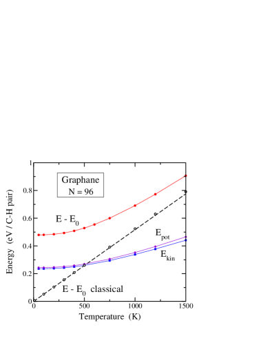
In Fig. 4 we present the internal energy of graphane as a function of temperature, as derived from our PIMD simulations (solid circles). As noted in Sec. II.A, PIMD simulations yield separately the potential ($E_{\rm pot}$) and kinetic ($E_{\rm kin}$) contributions to the internal energy $E$ Herman et al. (1982); Tuckerman (2010); Herrero and Ramírez (2014), so that for $\tau=0$ we have $E-E_{0}=E_{\rm kin}+E_{\rm pot}$. Solid squares and diamonds in Fig. 4 correspond to the kinetic and potential energy, respectively. The internal energy $E-E_{0}$ is found to converge at low $T$ to 479 meV/(C–H pair), which gives the zero-point energy of the system. For comparison, we also display in Fig. 4 results of the internal energy obtained in classical MD simulations (open circles). These data points lie very close to the classical harmonic expectation, i.e., $E^{\rm cl}-E_{0}=6k_{B}T$ per C–H pair. For $T\gtrsim 1000$ K we observe a slight deviation of the simulation results from the harmonic expectancy, because of the onset of anharmonicity. At high temperatures, the energy obtained from quantum simulations converges to that of classical MD simulations. At $T=1500$ K, however, one still sees a significant difference between classical and quantum energy values.

For a purely harmonic model of the vibrational modes, one has $E_{\rm kin}=E_{\rm pot}$ (virial theorem Landau and Lifshitz (1980); Feynman (1972)), irrespective of temperature in both classical and quantum approaches. In our simulations of graphane, a ratio $E_{\rm kin}/E_{\rm pot}=1$ is obtained for the classical model in the low-temperature limit, as in this case the atomic motion does not explore the energy landscape far from the absolute minimum, because of the vanishingly small vibrational amplitudes. This does not happen for the quantum results in the limit $T\to 0$, since in this case the vibrational amplitudes remain finite, thus feeling the anharmonicity of the interatomic potential.

In the quantum results we observe that $E_{\rm pot}>E_{\rm kin}$ in the whole temperature range shown in Fig. 4. The difference $E_{\rm pot}-E_{\rm kin}$ increases for rising $T$, and remains positive in the low-temperature limit. For $T\to 0$ we find a difference of 8 meV/(C–H pair). This is basically due to the zero-point expansion of graphane in both the out-of-plane and in-plane directions (an anharmonic effect), which causes an increase of the potential energy with respect to the minimum energy configuration. At 1500 K the difference $E_{\rm pot}-E_{\rm kin}$ amounts to 24 meV per C–H pair, i.e., three times larger than at low $T$. The data presented in Fig. 4 correspond to $N=96$. For other cell sizes we obtained results for the internal energy very close to those given for $N=96$, and are indistinguishable one from the other at the scale of the figure.

Figure 5: Kinetic energy of hydrogen (solid squares) and carbon atoms (solid circles) vs the temperature, as derived from PIMD simulations of graphane. Open diamonds indicate the kinetic energy of carbon atoms in graphene. The dashed line represents the classical limit of the kinetic energy per atom in a harmonic approximation: $E_{\rm kin}^{\rm cl}=3k_{B}T/2$. Solid and dotted lines are guides to the eye.

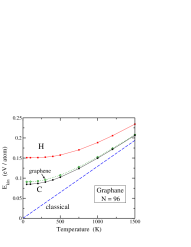
The kinetic energy of hydrogen and carbon atoms is displayed vs the temperature in Fig. 5. Solid symbols represent results of PIMD simulations of graphane: squares for H and circles for C. At low temperature, the kinetic energy for C is about one half of that for H. This difference is reduced for increasing $T$, since the kinetic energy converges to the classical limit at high temperature. The dashed line in Fig. 5 represents the classical kinetic energy per atom: $E_{\rm kin}^{\rm cl}=3k_{B}T/2$. In this figure we have also plotted $E_{\rm kin}$ for C atoms in graphene (open diamonds). At low $T$ it is somewhat larger than that corresponding to C atoms in graphane (6 meV/atom). The smaller value of $E_{\rm kin}$ in graphane is mainly due to a softening of vibrational modes such as C–C stretching ($sp^{3}$ hybridization in graphane vs $sp^{2}$ in graphene) Ramírez and Herrero (2019).

A splitting of the potential energy of graphane into contributions of hydrogen and carbon, similar to that presented for the kinetic energy, is not directly feasible from the results of PIMD simulations. The virial estimator employed here to calculate $E_{\rm kin}$ (see Sec. II.A) yields separately the contributions of H and C atoms. However, the Hamiltonian corresponding to the TB method does not allow to express independent inputs for the potential energy of both species. An indirect method to split $E_{\rm pot}$ could be based on a separation into different vibrational modes of graphane, but this would require to deal with a harmonic approximation for the modes, as well as for the splitting of the energy of each mode into the H and C parts.

A quantification of the overall anharmonicity in graphene can be found from the relation between $E_{\rm kin}$ and $E_{\rm pot}$. From the data presented above we find a ratio $E_{\rm pot}/E_{\rm kin}=$ 1.03 for low temperature, which slowly increases for rising $T$, reaching a value of 1.06 at 1500 K. Concerning the anharmonicity at low $T$, it is noteworthy that earlier analyses based on quasiharmonic approximations and perturbation theory indicate that the low-temperature changes in the vibrational energy with respect to a harmonic calculation are mostly due to the kinetic energy. This is due to the fact that for a perturbed harmonic oscillator at $T=0$, the first-order change in the energy is given by a variation of $E_{\rm kin}$, while $E_{\rm pot}$ is invariable with respect to its unperturbed value Landau and Lifshitz (1965); Herrero and Ramírez (1995). In particular, this has been observed for the vibrational energy of graphene at low temperature Herrero and Ramírez (2016). In the results presented here for graphane we find $E_{\rm pot}>E_{\rm kin}$, since the potential energy includes an important anharmonic contribution due to changes in the layer area, even at $T=0$ with respect to the classical minimum (see Sec. VII). The contribution of this elastic energy is not negligible, even at low temperature, and can be obtained for a single layer of graphene by reference to a strictly flat sheet, but it is not straightforwardly found for graphane which displays a finite lateral dimension even for the classical minimum-energy configuration.

IV Interatomic distances

Figure 6: Temperature dependence of mean interatomic distances in graphane. (a) C–C distance; (b) C–H distance. Solid circles and squares represent results of classical and PIMD simulations, respectively. Diamonds in (b) indicate the C–H distance for a single H atom on graphene. Lines are guides to the eye. Error bars are less than the symbol size.

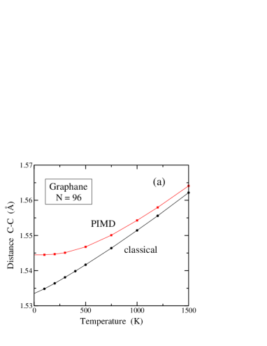
Here we present results for interatomic distances in graphane. In Fig. 6(a) we show the temperature dependence of the equilibrium C–C distance, $d_{\rm C-C}$, yielded by our PIMD simulations (solid squares). In the low-temperature limit $T\to 0$, we find an interatomic distance of 1.5445 Å, typical of a C–C single bond, which increases for rising temperature. The size effect of the finite simulation cells on $d_{\rm C-C}$ is negligible. For $N$ = 96 and 216 we obtained differences similar to the error bars found for each cell size (less than the symbol size in Fig. 6(a)). We note that PIMD simulations of graphene using the TB model employed here yielded a zero-temperature interatomic distance $d_{\rm C-C}$ = 1.4287 Å, intermediate between a single and a typical double bond ($\sim 1.34$ Å).

For comparison with the interatomic distances derived from the quantum simulations, we also display in Fig. 6(a) the temperature dependence of $d_{\rm C-C}$, as obtained from classical MD simulations (circles). These data show at low temperature a nearly linear increase, as expected for interatomic distances and lattice parameters of crystalline solids in a classical approximation Kittel (1966); Herrero and Ramírez (2000). The classical results for $d_{\rm C-C}$ of graphane converge at low temperature to an interatomic distance of 1.5337 Å, corresponding to the minimum energy configuration of graphane. This value is close to the distance $d_{\rm C-C}$ given by ab-initio calculations at $T=0$ Cadelano et al. (2010). Our PIMD simulations predict at low $T$ a C–C distance larger than the classical calculation, due to zero-point motion of the carbon atoms along with anharmonicity of the interatomic potential. Thus, for $T\to 0$ we find a zero-point expansion of the C–C bond by $1.1\times 10^{-2}$ Å, which means an increase of a 0.7% with respect to the classical value. We note that this rise in mean bond length due to nuclear quantum effects is much larger than the precision reached in the determination of interatomic distances from diffraction techniques Yamanaka et al. (1994); Ramdas et al. (1993); Kazimorov et al. (1998).

The bond expansion caused by nuclear quantum effects is reduced for rising temperature, as at high $T$ the quantum and classical predictions should approach one to the other. Nevertheless, at 1500 K the C–C distance derived from PIMD simulations is still clearly larger than that found in the classical simulations. The increase in $d_{\rm C-C}$ obtained in PIMD simulations from $T=0$ to room temperature is small, amounting to $\sim 6\times 10^{-4}$ Å, i.e., about 27 times less than the zero-point expansion. Moreover, the zero-point bond expansion is similar to the thermal expansion predicted by the classical model from $T=0$ to 650 K.

For comparison with the C–C distance in graphane, we note that the TB potential employed here yields for a single layer of graphene in the low-$T$ limit: $d_{\rm C-C}$ = 1.4192 Å and 1.4265 Å  from classical and PIMD simulations, respectively. This represents in the case of graphene a zero-point bond expansion of a 0.5% with respect to the classical prediction, somewhat less than for the relatively softer C–C bond in graphane.

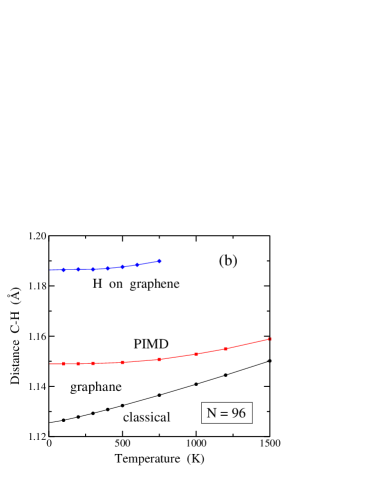
In Fig. 6(b) we present the C–H bond distance in graphane vs the temperature. As in Fig. 6(a) circles and squares are data points obtained from classical MD and PIMD simulations, respectively. The classical results converge at low $T$ to 1.1257 Å, a value close the result of ab-initio calculations Sahin et al. (2010); Huang and Zeng (2013); Chechin et al. (2014), while the low-temperature PIMD data yield $d_{\rm C-H}$ = 1.1490 Å. This means a zero-point expansion of 0.023 Å, i.e., a 2% of the bond length. Note the larger relative increase in bond distance compared with the C–C bond (a 0.7%), due essentially to the light mass of hydrogen.

We also show in Fig. 6(b) the distance C–H for a single hydrogen impurity on graphene Herrero and Ramírez (2009), as derived from PIMD simulations, for comparison with the results for graphane. For the single impurity, $d_{\rm C-H}$ is clearly larger than in the case of graphane, converging to 1.1863 Å for $T\to 0$. This larger distance reflects a weakening of the C–H bond with respect to the C–H bonds in graphane, where carbon atoms display an $sp^{3}$ hybridization. For a single hydrogen, however, the C atom adjacent to H presents a local configuration intermediate between that required by planar graphene ($sp^{2}$ hybridization) and tetrahedral $sp^{3}$ adequate for the C–H bond. In our simulations, a single hydrogen on graphene is found to diffuse along the simulations at $T\sim 1000$ K, so that a precise value for the C–H bond distance cannot be obtained at these temperatures.

The general trend of classical and quantum data for $d_{\rm C-C}$ in a graphane layer is qualitatively similar to that found in simulations of 3D carbon-based materials such as diamond Herrero and Ramírez (2000), as well as in graphene Herrero and Ramírez (2016). The thermal bond expansion along with the zero-point dilation presented here are an indication of anharmonicity in the interatomic potential. For C–C and C–H bonds in graphane, these effects are mainly due to anharmonicity in the corresponding stretching vibrations. A more complex anharmonic effect emerges in the explanation of thermal variations in the in-plane area of 2D materials such as graphane, because of the contributions of in-plane and out-of-plane modes, as discussed below in Sec. VII.

V Orientation of the C–H bonds

To analyze the orientation of the C–H bonds we will consider spherical coordinates $(\theta,\phi)$. The polar angle $\theta$ is defined as the angle between the $z$-direction and the C–H bond, and $\phi$ is the azimuth on the $(x,y)$ plane. In the minimum-energy configuration we find $\theta=0$, i.e., the C–H bond is strictly perpendicular to the $(x,y)$ plane.

Figure 7: Mean polar angle $\langle\theta\rangle$ between the C-H bond and the $z$-direction as a function of temperature. Symbols indicate results of simulations: circles, classical MD; squares, PIMD. Lines are guides to the eye. Error bars are in the order of the symbol size.

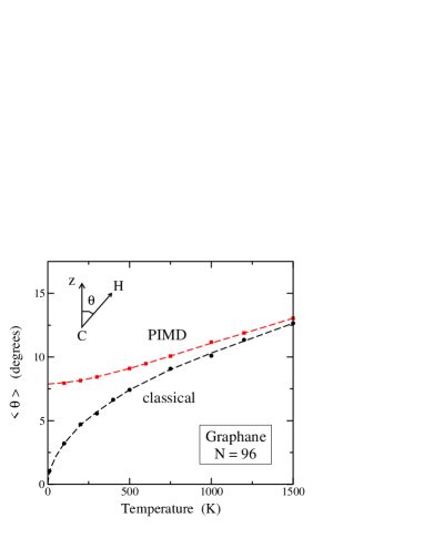
In Fig. 7 we display the mean value of the polar angle, $\langle\theta\rangle$, for graphane as a function of temperature. Shown are results derived from classical (circles) and PIMD (squares) simulations. In the classical approach we find that $\langle\theta\rangle$ converges to zero at low temperature as $\sqrt{T}$. In fact, we find a dependence $\langle\theta\rangle^{2}=\gamma T$ with a coefficient $\gamma$ = 0.110 deg²/K. The PIMD results converge to a finite value for $T\to 0$: $\langle\theta\rangle_{0}$ = 7.8 deg due to zero-point motion. $\langle\theta\rangle$ increases as temperature is raised and reaches a value of 13.0 deg for $T$ = 1500 K. At this temperature the classical and quantum results are close one to the other.

Our results for $\langle\theta\rangle$ can be related with the probability distribution for the direction of the C–H bond in the whole sphere. We describe the orientation of the C–H axis by the probability density $P(\theta,\phi)$, which verifies the normalization condition:

$$\int_{0}^{2\pi}d\phi\int_{0}^{\pi}P(\theta,\phi)\sin\theta\,d\theta=1\,.$$ (7)

Although $P(\theta,\phi)$ could depend on the azimuthal angle $\phi$, we find a uniform distribution for $\phi\in[0,2\pi]$, i.e. we observe a density with cylindrical symmetry around the $z$ axis (changes in the probability density for different angles $\theta$ are less than 3%). Thus, we can define an average density

$$\bar{P}(\theta)=\int_{0}^{2\pi}P(\theta,\phi)\,d\phi\,,$$ (8)

which depends only on the polar angle $\theta$.

The results of our simulations, both classical and quantum, indicate that $\bar{P}(\theta)$ follows very closely (i.e., within the statistical noise) a Gaussian distribution:

$$\bar{P}(\theta)=c\,\exp(-a\theta^{2})\,,$$ (9)

where $c$ is a normalization constant given by

$$c^{-1}=\int_{0}^{\pi}\sin\theta\,\exp(-a\theta^{2})\,d\theta\,.$$ (10)

The parameter $a$ in Eq. (9) controls the width of the Gaussian distribution. It decreases for increasing $T$ as the density distribution becomes wider. From the results of our PIMD simulations, we find $a$ = 40.6 and 14.8 rad^-2 for $T$ = 100 and 1500 K, respectively.

In the classical approach, the parameter $a$ diverges for $T\to 0$, and the Gaussian in Eq. (9) converges to a Dirac $\delta$-function. Then, the C–H bonds are strictly perpendicular to the $(x,y)$ layer plane, as indicated above. In general, the mean polar angle $\langle\theta\rangle$ can be written as

$$\langle\theta\rangle=\int_{0}^{\pi}\bar{P}(\theta)\,\theta\,\sin\theta\,d\theta\;.$$ (11)

In the quantum approach we find a zero-temperature limit $\langle\theta\rangle_{0}$ = 0.136 rad = 7.8 deg, which corresponds to a parameter $a_{0}$ = 42.2 rad^-2.

VI Atomic motion

In this section we present results for the MSD of C and H atoms in graphane. We concentrate on the nature of the atomic displacements, to find out if they may be described by classical motion or the atoms largely behave as quantum particles. We expect that a quantum model will be more appropriate at low temperature, not only for H, but also for the relatively heavier C atoms. We employ the notation presented in Sec. II.C.

Figure 8: Atomic mean-square displacements in the in-plane $x$-direction. (a) Carbon atoms: Symbols are data points obtained from PIMD simulations for graphane (solid circles) and graphene (open diamonds). (b) Hydrogen atoms: Symbols are data points derived from classical (circles) and PIMD simulations (squares). These results were obtained for a graphane cell containing 216 C-H pairs. Lines are guides to the eye.

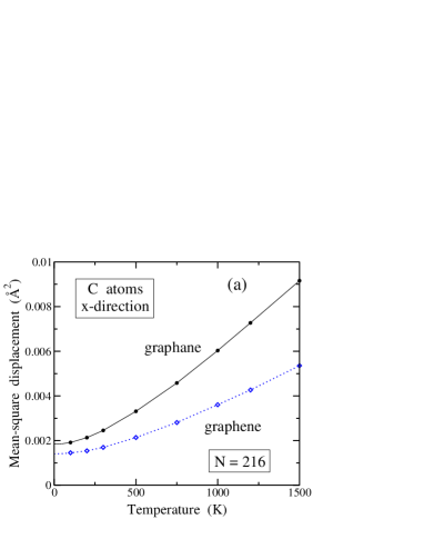
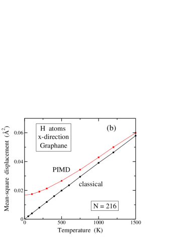
In Fig. 8 we show the MSD of C and H atoms on the $(x,y)$ plane. Results for the $x$ and $y$ directions turn out to be indistinguishable, so we present only those found in the $x$-direction. These data were obtained for a simulation cell with $N$ = 216. In Fig. 8(a) we display the MSD of C atoms as derived from PIMD simulations of graphane (solid circles). For comparison we also present the MSD of carbon atoms in graphene, obtained by using the same TB model. The MSD is clearly larger in the case of graphane, reflecting a softer effective in-plane potential for the motion of C atoms in the $(x,y)$ plane. In other words, this is due to a reduction in the vibrational frequencies of in-plane acoustic modes LA and TA in graphane with respect to graphene Ramírez and Herrero (2019), which causes larger amplitudes in the former case.

In Fig. 8(b) we display the mean-square displacement $(\Delta x)_{\rm H}^{2}$ of hydrogen atoms in graphane as a function of temperature. Shown are data points obtained from classical (circles) and PIMD (squares) simulations. The quantum results converge at low $T$ to a value $(\Delta x)_{0}^{2}=0.017$ Ų. Comparing the room-temperature data ($T=300$ K), we find that the quantum result is 1.8 times larger than the classical one. This ratio increases as the temperature is lowered, and at 100 K it amounts to 4.3. Comparing the quantum results for the MSD of C and H atoms in graphane at room temperature, we find that the former is about 9 times smaller than the latter.

Figure 9: Temperature dependence of the mean-square displacements along the out-of-plane direction: classical $C_{z}^{2}$ (solid symbols) and quantum $Q_{z}^{2}$ (open symbols). In both cases, circles correspond to hydrogen and squares to carbon atoms. These results were obtained for a graphane cell containing 24 C-H pairs. Lines are guides to the eye.

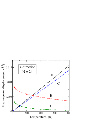
We now turn to the out-of-plane motion. This motion is relevant for several properties of 2D materials, as it controls the appearance of bending and crumpling in their constituent layers. In Fig. 9 we present results for the MSD of H and C in the $z$-direction, obtained for a graphane cell with $N=24$. The reason for presenting here results corresponding to a cell size smaller than in previous figures is that for $N=24$ one can visualize more clearly the competition between quantum and classical contributions to the MSD. As explained in Sec. II.C, this displacement may be divided into two parts: one of them quantum in nature, which corresponds to the spread of the quantum paths, $Q_{z}^{2}$ (open symbols), and another of classical character, which accounts for motion of the centroid (global displacements of the paths), $C_{z}^{2}$ (solid symbols). For $T\to 0$, $C_{z}^{2}$ vanishes and $Q_{z}^{2}$ converges to zero-point values of 3.9 and $9.1\times 10^{-3}$ Ų for C and H, respectively. $Q_{z}^{2}$ decreases for rising $T$, as the spatial extension of the quantum paths decreases, while $C_{z}^{2}$ grows almost linearly, in accord with the expectancy for the MSD of classical particles.

For the system size shown in Fig. 9 (N = 24), both terms contributing to $(\Delta z)^{2}$ are nearly equal at $T$ = 105 K and 280 K for carbon and hydrogen, respectively. For each element, at higher temperatures the classical contribution $C_{z}^{2}$ dominates the atomic displacements on the $z$-direction. The actual quantum delocalization of the atoms in the out-of-plane direction can be estimated from the “mean extension,” $(\Delta z)_{Q}$, of the quantum paths in this direction. At 300 K our simulations yield an average extension $(\Delta z)_{Q}=(Q_{z}^{2})^{1/2}$ = 0.030 and 0.073 Å, for carbon and hydrogen, respectively. This mean extension increases with lowering temperature, and for $T\to 0$, $(\Delta z)_{Q}$ amounts to 0.062 Å for C and 0.095 Å for H atoms.

At finite temperatures, the MSD in the out-of-plane direction, $(\Delta z)^{2}$, increases much faster than $(\Delta x)^{2}$, as a consequence of the rise in the classical contribution $C_{z}^{2}$ in the $z$ direction. This is due to the presence of long-wavelength vibrational modes with low frequency and large vibrational amplitudes in the ZA flexural band (atomic displacements in the $z$-direction). Calling ${\bf k}=(k_{x},k_{y})$ the wavevectors in the 2D reciprocal lattice of graphane Ramírez and Herrero (2019), this phonon band can be described at finite temperatures by a dispersion relation of the form $\rho\,\omega({\bf k})^{2}=\sigma k^{2}+\kappa k^{4}$, where $k=|{\bf k}|$, $\rho$ is the surface mass density, $\sigma$ an effective stress, and $\kappa$ the so-called bending modulus Ramírez et al. (2016). For our present purposes, $\sigma$ is negligible and the flexural band may be considered as parabolic: $\omega({\bf k})\approx\sqrt{\kappa/\rho}\,k^{2}$. For the present TB model we find at $T=$ 300 K a bending modulus $\kappa$ = 1.4 eV Ramírez and Herrero (2019). For increasing system size $N$ there appear vibrational modes with longer wavelength $\lambda$. In practice, one has an effective cut-off $\lambda_{max}\approx L$, where $L=(NA_{p})^{1/2}$, and $A_{p}$ is the in-plane area per C atom (see below). Thus, we have $k_{min}=2\pi/\lambda_{max}$, which means $k_{min}\sim N^{-1/2}$.

For system sizes larger than $N$ = 24, the temperature dependence of the atomic MSD in the $z$ direction is similar to that shown in Fig. 9. The main difference is that the temperature range where $Q_{z}^{2}$ or $C_{z}^{2}$ is the dominant contribution to $(\Delta z)^{2}$ depends on $N$. This is caused by the enlargement of the classical part $C_{z}^{2}$ for rising size, while $Q_{z}^{2}$ is rather insensitive to $N$ (clear finite-size effects in $Q_{z}^{2}$ are only found for very small simulation cells). This is analogous to earlier observations in graphene Herrero and Ramírez (2016). For given system size $N$ and atomic species, the ratio $Q_{z}^{2}/C_{z}^{2}$ decreases for rising $T$, so that there appears a crossover temperature $T_{c}$ for which this ratio equals unity, as indicated above for $N=24$. The main difference with graphene is that in the case of graphane each species sets its own temperature scale (or $T_{c}$) for this purpose. In each case, for $T>T_{c}$ classical-like motion is the dominant contribution in the atomic MSD in the $z$ direction. For graphene, the temperature $T_{c}$ was found to decrease for increasing system size $N$ as a power-law Herrero and Ramírez (2016), such as $T_{c}\sim N^{-b}$ with an exponent $b=0.67$. With the present TB model, however, we cannot reach large system sizes to obtain a reliable value for the exponent $b$ in graphane.

The competition between $Q_{z}^{2}$ and $C_{z}^{2}$ as functions of the system size presented here does not emerge for the in-plane MSD, where the crossover temperature $T_{c}$ is rather insensitive to the system size. For motion in the $(x,y)$ plane, $Q_{x}^{2}$ and $C_{x}^{2}$ quickly converge for rising $N$ to their corresponding asymptotic limit, in a way similar to the MSD derived from vibrational motion in 3D solids Herrero and Ramírez (2014). The main difference between in-plane and out-of-plane vibrational motion in this context is the appearance of the flexural ZA band in the $z$-direction with its distinctive parabolic dispersion relation for small $k$, $\omega_{\rm ZA}\sim k^{2}$, different from usual acoustic modes with $\omega\sim k$ Ramírez and Herrero (2019).

A consistency check for the overall results of our quantum atomistic simulations of graphane can be found from the comparison of data corresponding to the coordinate and momentum space. This can be done through the MSDs in real space and the kinetic energy presented in Sec. III. In fact, according to Heisenberg’s uncertainty principle, $E_{\rm kin}$ should verify the relation $E_{\rm kin}\geq F$, with the function $F$:

$$F=\frac{\hbar^{2}}{8m}\left[(\Delta x)^{-2}+(\Delta y)^{-2}+(\Delta z)^{-2}\right]\,,$$ (12)

where $m$ is the particle mass (see the Appendix).

For a 3D harmonic oscillator, the ratio $E_{\rm kin}/F$ converges to unity for $T\to 0$ (ground state). In general, one can consider the function $F$ as a lower boundary for the kinetic energy of a quantum particle. From our PIMD simulations of graphane at 50 K, we find $F$ = 125 and 57 meV for H and C, respectively. These values are smaller than the corresponding kinetic energy per atom: $E_{\rm kin}$ = 149 and 86 meV, which give $E_{\rm kin}/F$ = 1.2 for hydrogen and 1.5 for carbon.

The ratio $E_{\rm kin}/F$ converges at low $T$ to a value higher than 1 when one has a frequency dispersion for the vibrational modes, as is usual in condensed matter. Thus, for the well-known Debye model of solids Kittel (1966), $E_{\rm kin}/F\to 1.125$ for $T\to 0$ (see the Appendix). For hydrogen in graphane we find at low-$T$ a ratio of 1.2, due to frequency dispersion and anisotropy of this material (in-plane vs out-of-plane modes), which causes an increase in $E_{\rm kin}/F$. For C atoms we obtain a higher value at 50 K, which indicates that in this case we are farther from the low-$T$ limit due to the larger atomic mass.

VII Layer area

The simulations (both classical MD and PIMD) presented here were carried out in the isothermal-isobaric ensemble, as explained in Sec. II.A. This means that in a simulation run we fix the number $N$ of C–H pairs, the temperature $T$, and the applied stress in the $(x,y)$ plane ($\tau=0$ in our simulations), thus allowing for changes in the area of the simulation cell on which periodic boundary conditions are applied.

Figure 10: Temperature dependence of the mean in-plane area $A_{p}$ of graphane. Solid symbols correspond to results of PIMD simulations for $N$ = 96 (circles) and 216 (squares). Open squares are data points derived from classical MD simulations for $N=216$. Error bars are less than the symbol size. Lines are guides to the eye.

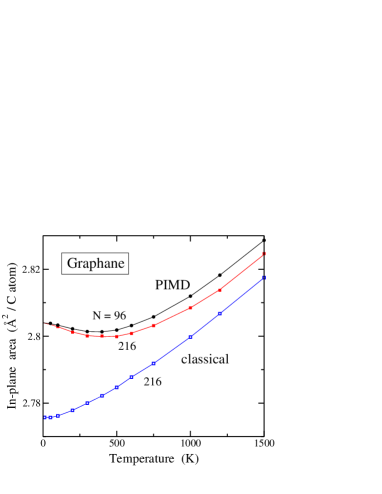
In Fig. 10 we present the temperature dependence of the in-plane area per C atom, $A_{p}=L_{x}L_{y}/N$, as derived from classical MD (open squares) and quantum PIMD simulations (solid squares) of graphane for $N=216$. For comparison we also display results from PIMD simulations for $N=96$. In the results of classical simulations we observe a slight decrease in $A_{p}$ at low $T$ (almost unobservable at the scale of Fig. 10), and at higher temperatures the in-plane area increases for rising $T$. In the low-$T$ limit, the classical in-plane area converges to the minimum-energy configuration with $A_{0}=2.7758$ Å². The general trend of these data is similar to that found in earlier classical Monte Carlo and MD simulations of graphene single layers Zakharchenko et al. (2009); Gao and Huang (2014); Brito et al. (2015). In the results of PIMD simulations we observe a clear decrease in $A_{p}$ from the low-temperature limit to $T\approx 400$ K, and a rise of $A_{p}$ at higher temperature.

The main difference between $A_{p}$ for different system sizes is a decrease in the in-plane area for rising cell size, but the temperature of the minimum $A_{p}$ is roughly unaffected. Notwithstanding the differences in the in-plane area per atom for the different system sizes, all of them converge in each case (quantum or classical) to a single value at low temperature. For $T\to 0$, the difference between $A_{p}$ derived from quantum and classical simulations amounts to 0.029 Ų/(C atom). This difference decreases as temperature is raised, since nuclear quantum effects become less important. At 1500 K it is $7\times 10^{-3}$ Ų/(C atom). Note that $dA_{p}/dT$ has to vanish for $T\to 0$, as required by the third law of Thermodynamics Callen (1960). This is the case for the results of PIMD simulations for graphane, and has been also discussed earlier for graphene Herrero and Ramírez (2016).

The behavior of $A_{p}$ as a function of temperature can be explained as due to two competing factors. On one side, there is a tendency of the C–C distance to increase for rising $T$ (see Fig. 6(a)), which favors a rise in $A_{p}$. On the other side, bending of the whole graphane layer gives rise to a reduction of its projection on the $(x,y)$ plane, i.e. the area $A_{p}$. For low temperature, the increase due to the first factor is dominated by the second one (bending), so that $dA_{p}/dT<0$. This is especially appreciable in the quantum results, since in this case the thermal expansion of the C–C bonds at low $T$ is small. At high temperatures, the rise in C–C distance dominates the reduction in the in-plane area due to out-of-plane atomic displacements, and we have $dA_{p}/dT>0$.

In connection with changes in the area $A_{p}$, we define the in-plane thermal expansion coefficient as

$$\alpha_{p}=\frac{1}{A_{p}}\left(\frac{\partial A_{p}}{\partial T}\right)_{\tau}\,.$$ (13)

which is negative at low $T$ and positive at high $T$, according to our PIMD simulations of graphane. $\alpha_{p}$ vanishes when the curve $A_{p}(T)$ has a minimum, i.e., for $T\approx 400$ K. At room temperature ($T=300$ K) we find $\alpha_{p}=-2.6\times 10^{-6}$ K^-1. Note, in contrast, that classical simulations yield at this temperature a positive coefficient $\alpha_{p}=7.8\times 10^{-6}$ K^-1.

For a single graphene layer, PIMD simulations with the TB model employed here yield a temperature dependence of the in-plane area analogous to that found earlier using effective interatomic potentials, such as the so-called LCBOPII (a long-range carbon bond-order potential) Herrero and Ramírez (2016). For graphene, the minimum area is found at $T\sim 1200$ K, a temperature much larger than that obtained for graphane. This important difference is due to the fact that the thermal expansion of the C–C bond in graphane is larger than that in graphene. Thus, at $T$ = 500 K we find an increase in $d_{\rm C-C}$ of $1.1\times 10^{-5}$ Å/K for graphane vs $4.4\times 10^{-6}$ Å/K for graphene, i.e, the former thermal expansion is a factor of 2.5 larger than the latter. At 1000 K we find a ratio of 2.3.

As a brief summary of the data presented in this section, we point out that changes in the in-plane area are important anharmonic effects, to which the PIMD procedure is very sensitive. At low temperatures, these anharmonic effects are appreciably enlarged by quantum motion, as shown in Fig. 10. This is caused by the fact that anharmonicity is revealed in the quantum model even at low $T$, in contrast to the classical case, where it progressively appears for rising temperature. We have also found that size effects in the in-plane area $A_{p}$ are much less important than in graphene.

VIII Compressibility

Important physical information about the intrinsic stability of 2D materails can be obtained by studying their mechanical properties. In particular, properties such as stiffness and bending rigidity can be affected by crumpling or corrugation of the layers Ruiz-Vargas et al. (2011); Kosmrlj and Nelson (2013, 2014), and are relevant for possible applications Seol et al. (2010); Prasher (2010). An interesting variable in this context is the 2D compressibility, which can be directly calculated from PIMD simulations.

The in-plane isothermal compressibility, $\chi_{p}$, at temperature $T$, is defined as

$$\chi_{p}=-\frac{1}{A_{p}}\left(\frac{\partial A_{p}}{\partial\tau}\right)_{T}\,.$$ (14)

In this equation, the variables in the r.h.s. correspond to in-plane variables, since the stress $\tau$ in the isothermal-isobaric ensemble employed here is a variable conjugate to the in-plane area $A_{p}$. The inverse of $\chi_{p}$, $B_{p}=1/\chi_{p}$, is the 2D modulus of hydrostatic compression Behroozi (1996), with units of eV/Ų or N/m. $B_{p}$ is the in-plane analogous to the bulk modulus of 3D solids.

An alternative way to calculate $\chi_{p}$ consists in using the fluctuation formula Landau and Lifshitz (1980); Ramírez and Herrero (2017)

$$\chi_{p}=\frac{N\sigma_{p}^{2}}{k_{B}TA_{p}}$$ (15)

where $\sigma_{p}^{2}$ are the mean-square fluctuations of the area $A_{p}$ obtained in the simulations. This expression turns out to be more adequate for our present purposes than obtaining $(\partial A_{p}/\partial\tau)_{T}$ as in Eq. (14), because a calculation of this derivative by numerical methods needs to carry out additional simulations at nonzero stresses. Thus, using Eq. (15) we can calculate the compressibility $\chi_{p}$ from our PIMD simulations with vanishing external stress ($\tau=0$). In any case, at some selected temperatures we have checked that both methods yield the same results for $\chi_{p}$, taking into account the statistical error bars.

Figure 11: Temperature dependence of the in-plane compressibility $\chi_{p}$, as obtained from PIMD simulations for graphane (circles) and graphene (squares). Dashed lines are guides to the eye. Error bars for the graphene data are in the order of the symbol size. Horizontal arrows with the label “class” indicate the zero-temperature classical limit for $\chi_{p}$.

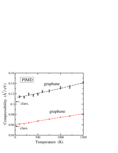
In Fig. 11 we show the temperature dependence of the compressibility $\chi_{p}$ for graphane (circles), as derived from our stress-free PIMD simulations. For comparison we also present results for graphene obtained with the same method (squares). Error bars for $\chi_{p}$ of graphane are about two or three times larger than those for graphene, as a consequence of the larger values of $\sigma_{p}^{2}$ for the latter, i.e., fluctuations in $\chi_{p}$ rise when its mean value increases.

The classical value of the in-plane compressibility at $T=0$ is given by

$$\chi_{0}=\frac{1}{A_{0}}\left(\frac{\partial^{2}E}{\partial A_{p}^{2}}\right)_{0}^{-1}\;,$$ (16)

where the subscript “0” indicates that the derivative is taken at the minimum-energy configuration (area $A_{0}$). Horizontal arrows in Fig. 11 indicate the classical zero-temperature limit $\chi_{0}$ for graphane and graphene. We find that the compressibility appreciably rises when nuclear quantum effects are taken into account. In the low-temperature limit, $\chi_{p}$ of graphane increases by a 9% with respect to the classical prediction, a relative growth similar to that found for graphene.

IX Summary

Graphane, as a quasi-2D material, displays typical properties of membranes, but a detailed study at the atomic scale yields important information about the effect of vibrational modes on the properties of this material. We have presented and discussed results of PIMD simulations of graphane in the isothermal-isobaric ensemble in a wide range of temperatures. This kind of simulations have revealed themselves as an adequate technique to study several properties of graphane layers. We have focused on the importance of nuclear quantum effects, which have been quantified by comparing results of the quantum simulations with those given by classical MD simulations. Our results indicate that explicit consideration of the quantum nature of atomic nuclei is important for a reliable description of these quasi-2D membranes, especially at low temperatures. Even for $T$ close to room temperature, such nuclear quantum effects are not negligible.

Several structural variables have been found to change when the quantum nature of atomic nuclei is taken into account. The interatomic distances and in-plane area appreciably increase with respect to the classical prediction. In the low-$T$ limit the mean C–C and C–H bonds increase by 0.7% and 2%, respectively. The higher value for the C-H bonds is indeed due to the lighter mass of hydrogen, combined with the anharmonicity of the interatomic potential.

Zero-point expansion of the graphane layer due to nuclear quantum motion amounts to about 1% for the in-plane area $A_{p}$. For $T>0$, a thermal contraction of $A_{p}$ is found for graphane in a similar way to graphene monolayers. However, it is important to note that in the case of graphane this contraction is almost unobservable in classical MD simulations. Thus, the temperature dependence of the area $A_{p}$ is qualitatively different when derived from classical or PIMD simulations at temperatures around 300 K and even higher (see Fig. 10). In the quntum simulations, the thermal expansion coefficient $\alpha_{p}$ is found to be negative for $T\lesssim$ 400 K, and it becomes positive at higher $T$.

The in-plane compressibility of graphane $\chi_{p}$ has been found to be about twice that of graphene, as a consequence of the tetrahedral (nonplanar) connectivity of the C atoms in graphane. $\chi_{p}$ appreciably rises when nuclear quantum motion is considered, and in the limit $T\to 0$, it is a 9% larger than the classical expectancy.

Atomic vibrations in the out-of-plane direction increase with both temperature and system size. Although quantum effects show up in these vibrational modes, at finite temperatures classical-like motion overshadows the quantum delocalization in the $z$-direction, as long as the system size is large enough. This size effect is observable in PIMD simulations at low temperatures, due to the onset of vibrational modes with smaller wavenumbers in larger cells, in particular in the ZA flexural band.

A quantitative assessment of the anharmonicity in the atomic vibrations is given by a comparison of the kinetic and potential energy of the system, which should coincide for strictly harmonic modes. For a graphane layer we find that $E_{\rm pot}>E_{\rm kin}$ in the whole temperature range studied here. The difference $E_{\rm pot}-E_{\rm kin}$ increases as $T$ is raised, and in the low-temperature limit it amounts to 8 meV/(C–H pair), i.e., a 3.5% of $E_{\rm kin}$. This is caused by the anharmonicity of the system at low $T$, as probed by the atomic zero-point motion.

PIMD simulations similar to those presented here can yield information on the structural and mechanical properties of graphane under tensile and compressive stress. This may give us insight into the relative stability of these layers in a stress-temperature phase diagram.

CRediT author contribution statement

Carlos P. Herrero: Data curation, Investigation, Validation, Original draft

Rafael Ramírez: Methodology, Software, Investigation, Validation

Declaration of Competing Interest

The authors declare that they have no known competing financial interests or personal relationships that could have appeared to influence the work reported in this paper.

Appendix A Uncertainty relations

The RMS displacements of the position coordinate $x$ and momentum $p_{x}$ verify the Heisenberg’s uncertainty relation (see, e.g., Ref. Cohen-Tannoudji et al. (1977) complement C.III)

$$\Delta x\,\Delta p_{x}\geq\frac{\hbar}{2}\,,$$ (17)

and similar expressions are valid for the $y$ and $z$ coordinates. Taking into account that $\langle p_{x}\rangle=0$, then $(\Delta p_{x})^{2}=\langle p_{x}^{2}\rangle$, so that for a particle with mass $m$ we have:

$$E_{\rm kin}=\frac{\langle{\bf p}^{2}\rangle}{2m}=\frac{1}{2m}\left[(\Delta p_{x})^{2}+(\Delta p_{y})^{2}+(\Delta p_{z})^{2}\right]\,.$$ (18)

From the inequality in Eq. (17) it follows

$$(\Delta p_{x})^{2}\geq\frac{\hbar^{2}}{4(\Delta x)^{2}}\,,$$ (19)

which yields

$$E_{\rm kin}\geq F\,,$$ (20)

$F$ being a function of the atomic MSDs:

$$F=\frac{\hbar^{2}}{8m}\left[(\Delta x)^{-2}+(\Delta y)^{-2}+(\Delta z)^{-2}\right]\,.$$ (21)

This means that we have a lower boundary for the kinetic energy from the real-space delocalization.

For an isotropic 3D harmonic oscillator wiht frequency $\omega$, we have for the ground state:

$$(\Delta x)^{2}_{0}=\frac{\hbar}{2m\,\omega}\,,$$ (22)

and

$$(E_{\rm kin})_{0}=\frac{3}{4}\hbar\,\omega\,,$$ (23)

so that $E_{\rm kin}/F$ converges to unity in the low-temperature limit.

To take into account the dispersion of frequencies in condensed matter, we can consider an isotropic 3D Debye model Kittel (1966) with a vibrational density of states $\mu(\omega)\propto\omega^{2}$ and a high-frequency cutoff $\omega_{D}$. In this case, assuming harmonic vibrations, we find for $T\to 0$:

$$(\Delta x)^{2}_{0}=\frac{3}{\omega_{D}^{3}}\int_{0}^{\omega_{D}}\frac{\hbar}{2m\,\omega}\,\omega^{2}d\omega=\frac{3}{4}\,\frac{\hbar}{m\,\omega_{D}}\,,$$ (24)

and

$$(E_{\rm kin})_{0}=3\,\frac{(\Delta p_{x})^{2}_{0}}{2m}=\frac{9}{16}\hbar\,\omega_{D}\,.$$ (25)

Hence, in the low-$T$ limit the ratio $E_{\rm kin}/F$ for the Debye model is independent of $\omega_{D}$ and converges to 1.125.

References

- Geim and Novoselov (2007) A. K. Geim and K. S. Novoselov, Nature Mater. 6, 183 (2007).
- Woods et al. (2014) C. R. Woods, L. Britnell, A. Eckmann, R. S. Ma, J. C. Lu, H. M. Guo, X. Lin, G. L. Yu, Y. Cao, R. V. Gorbachev, et al., Nature Phys. 10, 451 (2014).
- Meunier et al. (2016) V. Meunier, A. G. Souza Filho, E. B. Barros, and M. S. Dresselhaus, Rev. Mod. Phys. 88, 025005 (2016).
- Castro Neto et al. (2009) A. H. Castro Neto, F. Guinea, N. M. R. Peres, K. S. Novoselov, and A. K. Geim, Rev. Mod. Phys. 81, 109 (2009).
- Cao et al. (2018) Y. Cao, V. Fatemi, S. Fang, K. Watanabe, T. Taniguchi, E. Kaxiras, and P. Jarillo-Herrero, Nature 556, 43 (2018).
- Yankowitz et al. (2019) M. Yankowitz, S. Chen, H. Polshyn, Y. Zhang, K. Watanabe, T. Taniguchi, D. Graf, A. F. Young, and C. R. Dean, Science 363, 1059 (2019).
- Sofo et al. (2007) J. O. Sofo, A. S. Chaudhari, and G. D. Barber, Phys. Rev. B 75, 153401 (2007).
- Wen et al. (2011) X.-D. Wen, L. Hand, V. Labet, T. Yang, R. Hoffmann, N. W. Ashcroft, A. R. Oganov, and A. O. Lyakhov, PNAS USA 108, 6833 (2011).
- Cadelano et al. (2010) E. Cadelano, P. L. Palla, S. Giordano, and L. Colombo, Phys. Rev. B 82, 235414 (2010).
- Elias et al. (2009) D. C. Elias, R. R. Nair, T. M. G. Mohiuddin, S. V. Morozov, P. Blake, M. P. Halsall, A. C. Ferrari, D. W. Boukhvalov, M. I. Katsnelson, A. K. Geim, et al., Science 323, 610 (2009).
- Sahin et al. (2010) H. Sahin, C. Ataca, and S. Ciraci, Phys. Rev. B 81, 205417 (2010).
- Wang et al. (2016a) L. Wang, Z. Sofer, D. Bousa, D. Sedmidubsky, S. Huber, S. Matejkova, A. Michalcova, and M. Pumera, Andgewandte Chemie Intern. Ed. 55, 13965 (2016a).
- Mapasha et al. (2017) R. E. Mapasha, M. P. Molepo, and N. Chetty, RSC Adv. 7, 39748 (2017).
- Eng et al. (2013) A. Y. S. Eng, H. L. Poh, F. Sanek, M. Marysko, S. Matejkova, Z. Sofer, and M. Pumera, ACS Nano 7, 5930 (2013).
- Safran (1994) S. A. Safran, Statistical Thermodynamics of Surfaces, Interfaces, and Membranes (Addison Wesley, New York, 1994).
- Nelson et al. (2004) D. Nelson, T. Piran, and S. Weinberg, Statistical Mechanics of Membranes and Surfaces (World Scientific, London, 2004).
- Tarazona et al. (2013) P. Tarazona, E. Chacón, and F. Bresme, J. Chem. Phys. 139, 094902 (2013).
- Fournier and Barbetta (2008) J.-B. Fournier and C. Barbetta, Phys. Rev. Lett. 100, 078103 (2008).
- Pop et al. (2012) E. Pop, V. Varshney, and A. K. Roy, MRS Bull. 37, 1273 (2012).
- Fong et al. (2013) K. C. Fong, E. E. Wollman, H. Ravi, W. Chen, A. A. Clerk, M. D. Shaw, H. G. Leduc, and K. C. Schwab, Phys. Rev. X 3, 041008 (2013).
- Wang et al. (2016b) P. Wang, W. Gao, and R. Huang, J. Appl. Phys. 119, 074305 (2016b).
- Herrero and Ramírez (2018a) C. P. Herrero and R. Ramírez, J. Chem. Phys. 148, 102302 (2018a).
- Costamagna et al. (2012) S. Costamagna, M. Neek-Amal, J. H. Los, and F. M. Peeters, Phys. Rev. B 86, 041408 (2012).
- Gao and Huang (2014) W. Gao and R. Huang, J. Mech. Phys. Solids 66, 42 (2014).
- Leenaerts et al. (2010) O. Leenaerts, H. Peelaers, A. D. Hernandez-Nieves, B. Partoens, and F. M. Peeters, Phys. Rev. B 82, 195436 (2010).
- Zhou et al. (2013) X. H. Zhou, Y. Huang, X. S. Chen, and W. Lu, Solid State Commun. 157, 24 (2013).
- Chechin et al. (2014) G. M. Chechin, S. V. Dmitriev, I. P. Lobzenko, and D. S. Ryabov, Phys. Rev. B 90, 045432 (2014).
- Liu et al. (2013) B. Liu, J. A. Baimova, S. V. Dmitriev, X. Wang, H. Zhu, and K. Zhou, J. Phys. D: Appl. Phys. 46, 305302 (2013).
- Gillan (1988) M. J. Gillan, Phil. Mag. A 58, 257 (1988).
- Ceperley (1995) D. M. Ceperley, Rev. Mod. Phys. 67, 279 (1995).
- Herrero and Ramírez (1995) C. P. Herrero and R. Ramírez, Phys. Rev. B 51, 16761 (1995).
- Ramírez and Herrero (2011) R. Ramírez and C. P. Herrero, Phys. Rev. B 84, 064130 (2011).
- Los et al. (2016) J. H. Los, A. Fasolino, and M. I. Katsnelson, Phys. Rev. Lett. 116, 015901 (2016).
- Herrero and Ramírez (2000) C. P. Herrero and R. Ramírez, Phys. Rev. B 63, 024103 (2000).
- Ramírez et al. (2006) R. Ramírez, C. P. Herrero, and E. R. Hernández, Phys. Rev. B 73, 245202 (2006).
- Herrero and Ramírez (2007) C. P. Herrero and R. Ramírez, Phys. Rev. Lett. 99, 205504 (2007).
- Brito et al. (2015) B. G. A. Brito, L. Cândido, G.-Q. Hai, and F. M. Peeters, Phys. Rev. B 92, 195416 (2015).
- Hasik et al. (2018) J. Hasik, E. Tosatti, and R. Martonak, Phys. Rev. B 97, 140301 (2018).
- Herrero and Ramírez (2016) C. P. Herrero and R. Ramírez, J. Chem. Phys. 145, 224701 (2016).
- Davidson et al. (2014) E. R. M. Davidson, J. Klimes, D. Alfe, and A. Michaelides, ACS Nano 8, 9905 (2014).
- Herrero and Ramírez (2009) C. P. Herrero and R. Ramírez, Phys. Rev. B 79, 115429 (2009).
- Huang and Zeng (2013) L. F. Huang and Z. Zeng, J. Appl. Phys. 113, 083524 (2013).
- Feynman (1972) R. P. Feynman, Statistical Mechanics (Addison-Wesley, New York, 1972).
- Kleinert (1990) H. Kleinert, Path Integrals in Quantum Mechanics, Statistics and Polymer Physics (World Scientific, Singapore, 1990).
- Chandler and Wolynes (1981) D. Chandler and P. G. Wolynes, J. Chem. Phys. 74, 4078 (1981).
- Tuckerman (2010) M. E. Tuckerman, Statistical Mechanics: Theory and Molecular Simulation (Oxford University Press, Oxford, 2010).
- Herrero and Ramírez (2014) C. P. Herrero and R. Ramírez, J. Phys.: Condens. Matter 26, 233201 (2014).
- Ramírez and Herrero (2017) R. Ramírez and C. P. Herrero, Phys. Rev. B 95, 045423 (2017).
- Shiba et al. (2016) H. Shiba, H. Noguchi, and J.-B. Fournier, Soft Matter 12, 2373 (2016).
- Herrero and Ramírez (2018b) C. P. Herrero and R. Ramírez, Phys. Rev. B 97, 195433 (2018b).
- Martyna et al. (1999) G. J. Martyna, A. Hughes, and M. E. Tuckerman, J. Chem. Phys. 110, 3275 (1999).
- Martyna et al. (1996) G. J. Martyna, M. E. Tuckerman, D. J. Tobias, and M. L. Klein, Mol. Phys. 87, 1117 (1996).
- Herrero et al. (2006) C. P. Herrero, R. Ramírez, and E. R. Hernández, Phys. Rev. B 73, 245211 (2006).
- Herman et al. (1982) M. F. Herman, E. J. Bruskin, and B. J. Berne, J. Chem. Phys. 76, 5150 (1982).
- Porezag et al. (1995) D. Porezag, T. Frauenheim, T. Köhler, G. Seifert, and R. Kaschner, Phys. Rev. B 51, 12947 (1995).
- Goringe et al. (1997) C. M. Goringe, D. R. Bowler, and E. Hernández, Rep. Prog. Phys. 60, 1447 (1997).
- Johnson et al. (1993) B. G. Johnson, P. M. W. Gill, and J. A. Pople, J. Chem. Phys. 98, 5612 (1993).
- López-Ciudad et al. (2003) T. López-Ciudad, R. Ramírez, J. Schulte, and M. C. Böhm, J. Chem. Phys. 119, 4328 (2003).
- Böhm et al. (2001) M. C. Böhm, J. Schulte, E. Hernández, and R. Ramírez, Chem. Phys. 264, 371 (2001).
- Herrero and Ramírez (2010) C. P. Herrero and R. Ramírez, J. Phys. D: Appl. Phys. 43, 255402 (2010).
- Gillan (1990) M. J. Gillan, in Computer Modelling of Fluids, Polymers and Solids, edited by C. R. A. Catlow, S. C. Parker, and M. P. Allen (Kluwer, Dordrecht, 1990), p. 155.
- Landau and Lifshitz (1980) L. D. Landau and E. M. Lifshitz, Statistical Physics (Pergamon, Oxford, 1980), 3rd ed.
- Ramírez and Herrero (2019) R. Ramírez and C. P. Herrero, J. Chem. Phys. 151, 224107 (2019).
- Landau and Lifshitz (1965) L. D. Landau and E. M. Lifshitz, Quantum Mechanics (Pergamon, Oxford, 1965), 2nd ed.
- Kittel (1966) C. Kittel, Introduction to Solid State Physics (Wiley, New York, 1966).
- Yamanaka et al. (1994) T. Yamanaka, S. Morimoto, and H. Kanda, Phys. Rev. B 49, 9341 (1994).
- Ramdas et al. (1993) A. K. Ramdas, S. Rodriguez, M. Grimsditch, T. R. Anthony, and W. F. Banholzer, Phys. Rev. Lett. 71, 189 (1993).
- Kazimorov et al. (1998) A. Kazimorov, J. Zegenhagen, and M. Cardona, Science 282, 930 (1998).
- Ramírez et al. (2016) R. Ramírez, E. Chacón, and C. P. Herrero, Phys. Rev. B 93, 235419 (2016).
- Zakharchenko et al. (2009) K. V. Zakharchenko, M. I. Katsnelson, and A. Fasolino, Phys. Rev. Lett. 102, 046808 (2009).
- Callen (1960) H. B. Callen, Thermodynamics (John Wiley, New York, 1960).
- Ruiz-Vargas et al. (2011) C. S. Ruiz-Vargas, H. L. Zhuang, P. Y. Huang, A. M. van der Zande, S. Garg, P. L. McEuen, D. A. Muller, R. G. Hennig, and J. Park, Nano Lett. 11, 2259 (2011).
- Kosmrlj and Nelson (2013) A. Kosmrlj and D. R. Nelson, Phys. Rev. E 88, 012136 (2013).
- Kosmrlj and Nelson (2014) A. Kosmrlj and D. R. Nelson, Phys. Rev. E 89, 022126 (2014).
- Seol et al. (2010) J. H. Seol, I. Jo, A. L. Moore, L. Lindsay, Z. H. Aitken, M. T. Pettes, X. Li, Z. Yao, R. Huang, D. Broido, et al., Science 328, 213 (2010).
- Prasher (2010) R. Prasher, Science 328, 185 (2010).
- Behroozi (1996) F. Behroozi, Langmuir 12, 2289 (1996).
- Cohen-Tannoudji et al. (1977) C. Cohen-Tannoudji, B. Liu, and F. Lalöe, Quantum Mechanics, vol. 1 (Wiley, New York, 1977).