Fixed Points of Quantum Gravity
and the Dimensionality of the UV Critical Surface
Abstract
We study quantum effects in higher curvature extensions of general relativity using the functional renormalisation group. New flow equations are derived for general classes of models involving Ricci scalar, Ricci tensor, and Riemann tensor interactions. Our method is applied to test the asymptotic safety conjecture for quantum gravity with polynomial Riemann tensor interactions of the form and , and functions thereof. Interacting fixed points, universal scaling dimensions, gaps in eigenvalue spectra, quantum equations of motion, and de Sitter solutions are identified by combining high order polynomial approximations, Padé resummations, and full numerical integration. Most notably, we discover that quantum-induced shifts of scaling dimensions can lead to a four-dimensional ultraviolet critical surface. Increasingly higher-dimensional interactions remain irrelevant and show near-Gaussian scaling and signatures of weak coupling. Moreover, a new equal weight condition is put forward to identify stable eigenvectors to all orders in the expansion. Similarities and differences with results from the Einstein-Hilbert approximation, approximations, and models are highlighted and the relevance of findings for quantum gravity and the asymptotic safety conjecture is discussed.
I Introduction
Even more than a century after the discoveries of quantum mechanics and general relativity, an understanding of gravity as a fundamental quantum field theory of the metric field continues to offer challenges. Many proposals have been put forward to combine the principles of quantum physics with general relativity within and beyond quantum field-theoretical settings and include string theory, loop quantum gravity, asymptotically safe gravity, dynamical triangulations, matrix models, group field theory, causal sets, and more.
The asymptotic safety conjecture for gravity Weinberg:1980gg stipulates the existence of an interacting high-energy fixed point under the renormalisation group (RG) evolution of couplings Wilson:1971bg ; Wilson:1971dh ; Litim:2006dx ; Niedermaier:2006ns ; Litim:2011cp . Quantum effects turn gravitational couplings into running ones with a short-distance fixed point triggered by the anti-screening nature of gravity. Renormalisation group trajectories connect the short-distance quantum regime with the large-distance regime of classical general relativity, and a small set of fundamentally free parameters ensures predictivity. As such, asymptotic safety bears the promise to overcome the non-renormalisability of Einstein’s theory Goroff:1985sz ; Goroff:1985th ; Gomis:1995jp and the absence of asymptotic freedom in renormalisable fourth order extensions Stelle:1976gc ; Anselmi:2018ibi .
Proofs for asymptotic safety, however, are hard to come by. In four space-time dimensions, and without gravity, asymptotic safety for gauge-matter theories has recently been established rigorously both at weak Litim:2014uca ; Bond:2016dvk ; Buyukbese:2017ehm ; Bond:2017suy ; Bond:2017tbw ; Bond:2019npq and at strong coupling Bond:2022xvr using RG methods, also offering new directions for model building. Similarly, for certain perturbatively non-renromalisable theories- such as 3D theories with elementary four- or six-fermion interactions, asymptotic safety has also been established rigorously Rosenstein:1988pt ; deCalan:1991km ; Jakovac:2014lqa ; Cresswell-Hogg:2022lgg using large- techniques. For 4D quantum gravity, however, anomalous dimensions are expected to be large and a fixed point search requires non-perturbative tools. Still, canonical power counting can be used as a guiding principle for a bootstrap search Falls:2013bv , together with functional renormalisation Polchinski:1983gv ; Wetterich:1992yh ; Morris:1993qb ; Reuter:1996cp ; Freire:2000bq ; Litim:2001up . By now, strong circumstantial hints for asymptotic safety have been found in the Einstein Hilbert theory Souma:1999at ; Souma:2000vs ; Reuter:2001ag ; Lauscher:2001ya ; Litim:2003vp ; Bonanno:2004sy ; Fischer:2006fz ; Litim:2008tt ; Eichhorn:2009ah ; Manrique:2009uh ; Eichhorn:2010tb ; Manrique:2010am ; Manrique:2011jc ; Litim:2012vz ; Donkin:2012ud ; Christiansen:2012rx ; Codello:2013fpa ; Christiansen:2014raa ; Becker:2014qya ; Falls:2014zba ; Falls:2015qga ; Falls:2015cta ; Christiansen:2015rva ; Gies:2015tca ; Benedetti:2015zsw ; Biemans:2016rvp ; Pagani:2016dof ; Falls:2017cze ; Houthoff:2017oam ; Knorr:2017fus and higher curvature extensions Lauscher:2002sq ; Codello:2006in ; Codello:2007bd ; Machado:2007ea ; Codello:2008vh ; Benedetti:2009rx ; Benedetti:2009gn ; Benedetti:2010nr ; Niedermaier:2011zz ; Niedermaier:2009zz ; Niedermaier:2010zz ; Groh:2011vn ; Benedetti:2012dx ; Dietz:2012ic ; Ohta:2013uca ; Benedetti:2013jk ; Dietz:2013sba ; Falls:2014tra ; Saltas:2014cta ; Demmel:2014sga ; Eichhorn:2015bna ; Ohta:2015efa ; Ohta:2015fcu ; Demmel:2015oqa ; Falls:2016wsa ; Falls:2016msz ; Gies:2016con ; Christiansen:2016sjn ; Gonzalez-Martin:2017gza ; Becker:2017tcx ; Falls:2017lst ; Falls:2018ylp ; deBrito:2018jxt ; Falls:2020qhj . Intriguingly, high-order studies also observed that most quantum scaling dimensions become near-Gaussian despite of residual interactions, except for a few dominant ones, indicating that asymptotically safe quantum gravity becomes “as Gaussian as it gets” Falls:2013bv ; Falls:2014tra ; Falls:2017lst ; Falls:2018ylp .
In this paper, we investigate the impact of higher order curvature interactions for quantum gravity. There are several motivations for this. Firstly, higher curvature extensions have become of interest as extensions of classical general relativity, often in view of cosmology and inflation Sotiriou:2008rp ; DeFelice:2010aj ; Clifton:2011jh ; Capozziello:2011et , and holography Hung:2011xb . It is then natural to also investigate the impact of quantum fluctuations. Secondly, from the viewpoint of the asymptotic safety conjecture, higher order curvature interactions will be present rather naturally owing to residual interactions in the UV, and should therefore be taken into consideration. In particular, results in the Einstein-Hilbert or fourth order approximations require validation beyond the lowest orders of interaction monomials. Similarly, model studies which besides Einstein Hilbert terms only retain individual higher curvature invariants, often lead to very large scaling dimensions and should be revisited, e.g. Lauscher:2002sq ; Codello:2007bd ; Falls:2014tra ; Gies:2016con .
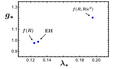
To analyse higher curvature invariants systematically, a bootstrap search strategy was introduced in Falls:2013bv . It relies on the hypothesis that canonical mass dimension remains a good ordering principle even at interacting fixed points, which is known to be true for fixed point systems observed in Nature. The virtue of this setup is that the validity of the hypothesis can be verified a posteriori, order by order in the approximation: If an additional operator with higher mass dimension is added, the newly introduced quantum scaling dimension should be more irrelevant than those found at the previous approximation order, while the remaining scaling dimensions are, at best, shifted by a small amount. The bootstrap strategy has first been used in models Falls:2014tra retaining monomials up to powers in curvature Falls:2018ylp . Most notably, the fixed point for Newton’s coupling and the cosmological constant come out close to the Einstein-Hilbert results, supporting the view that the latter is a faithful image of the fixed point in the full theory. On the other hand, the inclusion of high order Ricci tensor interactions Falls:2017lst has lead to more substantial shifts away from Einstein Hilbert results. As such, Fig. 1 illustrates clearly that the impact of higher order curvature interactions requires further scrutiny.
A third motivation for our work is the number of fundamentally free parameters of asymptotically safe gravity, also known as the dimension of the UV critical surface. In particular, one may wonder whether classically marginal or irrelevant interactions may become relevant quantum-mechanically. Thus far, the observed quantum shifts in the eigenvalue spectra compared to canonical values are typically of the order of a few. In principle, this pattern implies that some dim-6 invariants may very well become relevant in the quantum world. It also suggests that the number of fundamentally free parameters cannot be larger than the number of operators with mass dimension ; see Tab. 1 for a full list. Therefore, interaction monomials up to dim-6 are of particular interest if we want to understand the dimensionality of the UV critical surface. In practice, however, examples for any dim- interaction term to become relevant in quantum gravity have not yet been observed, either because quantum corrections are not large enough, or because they point into the irrelevant direction Falls:2014tra ; Falls:2017lst ; Falls:2018ylp . It is therefore important to check whether this remains true for approximations involving other dim- curvature invariants.
With these aims in mind, we derive new functional renormalisation group equations for models of quantum gravity involving Ricci scalar, Ricci tensor, and Riemann tensor interactions. The setup is rather general, and covers many higher curvature extensions of classical general relativity Sotiriou:2008rp ; DeFelice:2010aj ; Clifton:2011jh ; Capozziello:2011et . Our three-parameter families of quantum effective actions, once Taylor-expanded to high order, allow for systematic fixed point searches beyond Einstein Hilbert gravity. A key focus of this work are fixed points in new models of quantum gravity with high order Riemann tensor interactions, which are studied in depth. Results include fixed points, scaling dimensions, gaps in eigenvalue spectra, quantum equations of motion, de Sitter solutions, and the impact of Riemann interactions on the location of fixed points, complementing Fig. 1. We also study the new dim-6 curvature invariant which can become relevant at shortest distances. This feature is qualitatively new and different from the previously studied dim-6 invariants , , and the Goroff-Sagniotti term , and the implications are elaborated in detail.
Another novelty of our study is a first complete order-by-order analysis of eigenperturbations at fixed points. With the help of a new equal weight condition, we find that eigenperturbations are genuinely stable, and in accord with expectations from eigenvalue spectra. We also provide a detailed comparison of results with previous work and highlight similarities and differences due to different types of higher curvature interactions. On the technical side, we expand beyond previous efforts and use polynomial approximations of the action up to 144 orders in curvature, alongside Padé resummations and full numerical integration, to achieve our results.
| Curvature Invariants | |
|---|---|
| dim- | |
| dim- | |
| dim- | |
| dim- | |
The remainder of this work is organised as follows. In Sect. II we derive the main equations using functional renormalisation with a particular emphasis on Riemann tensor interactions, and lay out our fixed point search strategy. In Sect. III we discuss the main Riemann fixed point, its fixed point effective action, de Sitter solutions, and residuals. In Sect. IV, we find the universal scaling exponents and the UV critical surface. We also perform a bootstrap test and observe signatures of weak coupling. In Sect. V we detail our results for a pair of weakly coupled Riemann fixed points. In Sect. VI, we identify all eigenvectors and eigenperturbations for all fixed points by removing a rescaling ambiguity through a new equal weight condition. In Sect. VII we discuss the main features of our results and compare with earlier studies in different approximations. Finally, Sect. VIII gives a brief summary of our results and conclusions. Three appendices summarise technicalities such as first and second variations (Sect. A), Hessians (Sect. B), and the gravitational renormalisation group equations (Sect. C).
II Renormalisation Group for Gravity
In this section, we derive new functional renormalisation group equations for quantum gravity involving Riemann tensor interactions using heat kernel methods on spherical backgrounds. Our work completes a line of research initiated in Falls:2014tra ; Falls:2016wsa ; Falls:2017lst .
A Action
We are interested in gravitational actions of the form
| (1) |
with being an arbitrary dim-4 curvature invariant. and are a priori unspecified functions. The index indicates the Wilsonian RG scale at which the quantum effective action is evaluated. Ultimately, we are interested in the quantum effects induced by fluctuations of the metric fields, and the RG flow of the quantum effective action and the gravitational couplings contained in it, and its fixed points in the high energy limit. The most general form of can be written as
| (2) |
Since the overall normalisation of is irrelevant in that it can always be absorbed into a redefinition of coupling constants, only two out of the three parameters are truly independent.111A simple choice of independent parameters are the surface angles of the three-dimensional unit sphere spanned by the parameters . This slight redundancy is of no relevance for the present work and we will therefore stick to the parameters . The family of theories described by (1) with (2) contains the Einstein-Hilbert theory with scale-dependent cosmological constant and Newton’s coupling as the leading order coefficients
| (3) |
of a Taylor expansion in curvature. In the infrared limit the running couplings will have to agree with data, with Newton’s constant and with the cosmological constant . Besides being toy models for asymptotically safe gravity, actions of this type also arise as higher curvature extensions of classical general relativity, e.g. Sotiriou:2008rp ; DeFelice:2010aj ; Clifton:2011jh ; Capozziello:2011et .
A key feature of the models (1) with (2) is that a polynomial expansion of the action retains only a single curvature invariant with canonical mass dimension for any , whose RG flows are found unambiguously on spherical backgrounds Falls:2017lst . To make this statement more explicit, we construct a complete operator basis at any mass dimension containing the terms and together with operators vanishing on spherical backgrounds. One way to construct such a basis consists in using the scalar Ricci curvature together with the traceless Ricci tensor and the Weyl tensor. Assuming to be non-vanishing on the sphere, all operators of this basis except for and can be chosen to be proportional to at least one traceless Ricci or the Weyl tensor. Thus, all operators in this basis except for and vanish on a spherical geometry. In this way, spherical backgrounds can be used to project onto actions of the form (1) with (2) provided does not vanish on spheres (see also Kluth:2022vnq ). Effectively, in this setting the terms and act as representatives for higher order curvature invariants of dimension and , respectively. Hence, the corresponding actions on spheres takes the form
| (4) |
similar to the local potential approximation for -type gravity advocated in Benedetti:2012dx . In this light, our models are generalisations of the local potential approximation on maximally symmetric backgrounds, the main addition being that the underlying dynamics not only involves the Ricci scalar, but also the fluctuations due to Ricci and Riemann tensor interactions. We will sometimes refer to the functions as “rays” in the space of curvature invariants. In these conventions, the ray correspond to the conventional, -type, local potential approximation Benedetti:2012dx (see also Falls:2013bv ; Falls:2014tra ). The ray which involve Ricci tensor interactions have previously been investigated in Falls:2017lst . The ray which are sensitive to Riemann tensor interactions are the central subject of this study.
B Functional Renormalisation
Next, we derive the renormalisation group flow for general gravitational actions (1) with (2) using the method of functional renormalisation Wetterich:1992yh ; Reuter:1996cp in the context of gravity Litim:2008tt ; Litim:2011cp (see Percacci:2017fkn ; Reuter:2019byg for recent textbooks),
| (5) |
where is the gauge fixed effective average action, its second variation matrix and the regulator. A path integral representation for these classes of theories has been given in Falls:2017lst . Note that, within the background field method, this functional differential equation gives rise to a functional , depending on a background metric and some quantum fluctuation fields . We can rewrite this as
| (6) |
with
| (7) |
We then simplify this ansatz using the so called “single field” or “background field” approximation. This means, we impose that includes only terms of the bare action arising from the functional measure. Explicitly, this includes gauge fixing terms and ghost terms whose RG-running is neglected. Thus, they only enter on the right-hand side of (5) through the Hessian . Since the left-hand side then depends only on it is sufficient to evaluate the right-hand side at vanishing fluctuation fields , including . In addition, we choose the gauge fixing to be
| (8) |
with
| (9) |
Here, and the gauge parameter is chosen to be . Further, we split the background metric field from the quantum fields using a linear split,
| (10) |
where denotes the metric quantum fluctuation. Alternatively, one may use an exponential split as advocated in Kawai:1992np ; Kawai:1993mb (see also Nink:2014yya ; Falls:2015qga ; Falls:2015cta ) where the background field is split off the quantum field multiplicatively according to
| (11) |
In this case quadratic terms in the fluctuation field are retained and contribute both to the Hessians in (5) and the flow of couplings. In this work, and to make contact with previous studies, we adopt to the linear split (10) throughout. Moreover, the York decomposition is used to decompose the metric fluctuations according to
| (12) |
This ensures that no non-minimal differential operator will be present in the second variation matrix when evaluated on the sphere. Ghost contributions coming from this field redefinition as well as the gauge fixing term are denoted as such that
| (13) |
within our approximation. With these definitions we find for the flow equation
| (14) |
Here, traces w.r.t. spin fields (transverse traceless tensors) are denoted by , traces of spin fields (transverse vectors) by , and traces of scalar modes by . Primes are used to denote the exclusion of lowest modes in the calculation of these traces. At one loop accuracy, the flow equation can be integrated in closed form for any regulator to provide a regularised form of the full one loop effective action.
For the present purposes, we are interested in quantum effects beyond one loop. To that end, we choose the regulator for each Hessian according to the replacement rule
| (15) |
and denotes the momentum cutoff which we take to be the optimised cut-off Litim:2000ci ; Litim:2001up ; Litim:2003vp ,
| (16) |
The optimised cutoff function is key to finding explicit analytical expressions of flows Litim:2003vp . Cutoff functions where are termed type I, and those where are termed type II Codello:2008vh . For the flow equation (14) we use a type I cut-off for the fluctuations arising from the physical transverse and scalar modes of the graviton. However, using a type I cutoff for the terms arising from the gauge fixing and ghost contributions leads to spurious, convergence-limiting unphysical poles in the flow equation, for any real Ricci curvature Falls:2018ylp . Therefore, following Falls:2018ylp , these have been removed by using suitable type II cut-offs for the terms arising from the gauge fixing and ghost contributions, as can be seen explicitly from the two last traces in (14).
The first and second variations of as defined in (2) are given in App. A, see (A.2) and (A.3). The variations of the Ricci scalar curvature can be found in Falls:2017lst ; Percacci:2017fkn , for example, and the Hessians for and are given in App, B, see (B.1) and (B.2), respectively.
To obtain the final form of the flow equation, we define dimensionless functions and parameters through
| (17) |
with dimensionless variables and fields given by and , and calculate the traces using usual heat kernel techniques Avramidi:2000bm ; Falls:2017lst ; Kluth:2019vkg . Owing to the optimised cutoff only a finite set of heat kernel coefficients is required. More recently, all heat kernel coefficients on spheres in any dimension have been derived Kluth:2019vkg , which enables the use of more general cutoff functions. The resulting flow equation for general , which is the main new result of this section, takes the form
| (18) |
Terms on the RHS arise due to the canonical scaling of fields and variables, and due to quantum fluctuations. The explicit form of the fluctuation integrals is given in App. C. It is worth pointing out that due to the freedom of an overall rescaling of all couplings, models with parameters are physically equivalent to models with parameters , provided that , and a real number. We indicate this equivalence with the symbol “”. Flow equations in the special cases representing gravity, or representing certain types of higher order Ricci tensor interactions, have been given previously in Falls:2014tra ; Falls:2017lst ; Falls:2018ylp . For a path integral representation of the theory for all scales, see Falls:2017lst .
We remark that (18) is a coupled set of partial differential equations for two unknown functions and . The flow is partly disentangled by projecting onto the even and odd parts with respect to background curvature, leading to
| (19) |
The representation (19) is very convenient for numerical integrations of the flow. The flow equations (18) and (19) are a central new result of this study. They are put to work for Riemann tensor interactions in the following sections.
C Emergence of General Relativity
Prior to searching for quantum fixed points, it is interesting to show how classical general relativity emerges in the classical limit, following Falls:2014tra ; Falls:2017lst . Most importantly, while the renormalisation flows of the functions and mix on the quantum level, (19), the mixing is absent in the classical limit where the fluctuation integrals can be neglected ,
| (20) |
In this limit, the flow (20) is further simplified by introducing the new function
| (21) |
where on spheres, leading to
| (22) |
It states that all dimensionful couplings in the classical theory are independent of the energy scale. The flow (22) has the general solution
| (23) |
where the function is determined by the initial conditions for couplings at the reference scale . Classical fixed points are the -independent solutions of (23). A trivially -independent solution is achieved via the boundary condition const. It leads to a line of fixed points for classical theories of gravity with actions where , parametrized by the free parameter which in four space-time dimensions is a marginal coupling. The linearity of (22) also implies the existence of a Gaussian fixed point . Moreover, from the flow for the inverse,
| (24) |
we observe the existence of an infinite Gaussian fixed point Nicoll:1974zza
| (25) |
The Gaussian and infinite Gaussian fixed points arise from (23) in asymptotic UV and IR limits where , respectively Falls:2014tra ; Falls:2017lst .
We continue with the scaling analysis for monomials of degree in curvature. For these, the result (23) states that the corresponding coupling scales canonically with Gaussian exponents ,
| (26) |
Hence, the dimensionless vacuum energy term and the dimensionless Ricci scalar coupling are relevant operators, and their dimensionless couplings diverge towards the IR, leading to the infinite Gaussian fixed point (25) in the IR. Using (3) and and , we can relate the IR diverging couplings and to the dimensionless Newton coupling and the dimensionless cosmological constant as
| (27) |
In terms of these, the infinite Gaussian fixed point implies
| (28) |
in such a way that and are constants in the IR limit . We conclude that general relativity with positive or negative vacuum energy corresponds to the infinite Gaussian IR fixed point (28) provided that is positive or negative, respectively. Moreover, the infinite Gaussian fixed point is IR attractive in both couplings. The theory also displays an IR fixed point corresponding to a vanishing vacuum energy,
| (29) |
This fixed point is IR attractive in and IR repulsive in . Classically, it can only be achieved by fine-tuning the vacuum energy to zero through the boundary condition. This analysis can straightforwardly be extended to higher order monomials. According to (26), for all couplings with the Gaussian fixed point is IR attractive (repulsive) and therefore approached in the IR limit (UV limit), whereas the infinite Gaussian fixed point is IR repulsive (attractive) and therefore approached in the UV limit (IR limit).
Finally we emphasize that the emergence of classical general relativity as the infinite Gaussian fixed point (25) with (28) or (29) is consistent with the non-perturbative RG flow (19). The reason for this is that the fluctuation-induced contributions in (19) are parametrically suppressed over the classical contributions owing to in the limit , also recalling (21). Therefore, the limit (25) collapses the full RG flow onto the classical flow, which has general relativity with positive, negative, or vanishing cosmological constant amongst its low energy solutions, possibly amended by higher curvature interactions. The result is independent of the parameters . Previously, the emergence of classical general relativity as the infinite Gaussian fixed point of the functional RG flow has been shown for and models Falls:2014tra ; Falls:2017lst .
D Riemann Tensor Interactions
For the rest of this work, we fix the free parameters of the flow equation (18) to be
| (30) |
We recall that (30) represents the class of equivalent models with where is any real number. In terms of (2) this corresponds to the choice
| (31) |
For this setting, the first few leading terms of the gravitational effective action (1) in a polynomial expansion read
| (32) |
up to higher powers in curvature . For the fixed point search below, we retain interaction terms up to including and monomials, corresponding to a total of interaction terms in the effective action (32).
Most notably, this action involves new Riemann curvature invariants which have not been studied previously within the non-perturbative RG for gravity. The main purpose of this study is to establish whether the dynamics due to Riemann tensor interactions is going to affect the UV behaviour of the theory in any significant manner. Using a polynomial ansatz for (17) of the form
| (33) |
and evaluating everything on a spherical background, a series expansion in small dimensionless Ricci scalar curvatures is performed and equations containing the beta functions and the couplings of the theory are found. The parameter determines the number of different operators included in the effective average action (32).
At the fixed point, the beta functions vanish and the remainder of the flow equation (18) using (30) is given by
| (34) |
Performing a series expansion in we can bring the flow equation into the form
| (35) |
To fulfil this at any approximation order , all coefficients with must vanish. Hence, we are left with a system of algebraic equations which can be solved to find fixed points. In theories of gravity, the polynomial conditions can be solved recursively starting with a linear equation for from , and leading to unique expressions for all couplings in terms of two parameters ( which then need to be determined by other means Falls:2014tra . In our models, and ultimately due to the presence of fourth order propagating degrees of freedoms, it turns out that is quadratic in the highest coupling Falls:2017lst . In consequence, a recursive algebraic solution is more cumbersome wherefore we resort to a numerical method instead.
E Search Algorithm and Fixed Point Scan
After having derived the expressions , we need to solve them to find fixed points of the system. At any approximation order , we are given equations
| (36) |
depending on couplings . Thus, there are more open couplings than equations to solve and we need to impose boundary conditions on two of them. The effect of these boundary conditions on the fixed point solutions has been studied in Falls:2014tra . In our fixed point search algorithm, we follow the choice of standard boundary conditions given by
| (37) |
at each approximation order . Sometimes we refer to the choice (52) as ”free” boundary conditions for the fixed point search.
A recursive solution strategy to find the exact expressions for the fixed point couplings in gravity has been put forward in Falls:2014tra . Solving (36) provides us with expressions for the couplings in terms of the lower order couplings with . In theories, these lead to explicit expressions for couplings which reduce to algebraic expressions for all couplings with upon iteration (level 2) Falls:2013bv ; Falls:2014tra ; Falls:2018ylp . We emphasize that the expressions are algebraic throughout, the reason for this being that the first nontrivial equation is linear in the unknown quantity ( the coupling ). For theories with general Ricci tensor or Riemann tensor interactions such as here this is no longer the case and the leading equation becomes quadratic. One may still solve the recursive relations for each branch separately, though the expressions become impractical very fast. Alternatively, one may start with the next coupling in line, , which again obeys a linear equation. Upon iteration, we find closed algebraic expressions starting with (level 3). The quadratic condition giving is then exploited at the very end.
In this work, we perform a brute force numerical fixed point search. This can be initiated by using the fixed point in the Einstein-Hilbert approximation, the so-called Reuter fixed point, as a starting point Reuter:1996cp ; Souma:1999at ; Lauscher:2001ya ; Litim:2003vp . Then, we enhance the operator base and include the one with the smallest larger canonical mass dimension into the system, search for solutions in the vicinity of the previous fixed point coordinates, and repeat in the form of a bootstrap Falls:2013bv until some maximum order which we take to be . This strategy has worked well for gravity Falls:2013bv ; Falls:2014tra ; Falls:2018ylp and gravity Falls:2017lst , where the fixed point coupling remains close to its Einstein Hilbert value. In this sense, these and fixed points may be viewed as the higher order extension of the Reuter fixed point.
On the other hand, the system may very well have global fixed point solutions where Newton’s coupling and the cosmological constant differ sizeably from their Einstein-Hilbert values. We explore the latter possibility by modifying the search algorithm and adding random perturbations to the fixed point couplings at some order. By this token, we explore the possibility whether additional stable fixed points are available. If so, these new fixed point candidates are then further extended to higher orders, as before, using the bootstrap strategy. We also check that the thereby-found solutions, if any, do not depend on the order at which random perturbations in the initial values were added initially. Overall, these strategies allow us to scan a substantial portion of parameter space. As a word of caution, however, we stress that our search is not exhaustive. Due to the large parameter space there may still exist fixed points which have gone unnoticed in the numerical search, or fixed point solutions which defy the ordering principle set by canonical mass dimension Falls:2013bv .
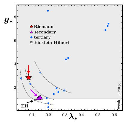
The result of our scan gives 23 fixed point candidates all of which have been computed consistently up to order in a first run.222We refer to these fixed points as “fixed point candidates” since they may contain spurious fixed point solutions. Thus, some of candidates may show instabilities in coupling coordinates. To illustrate the parameter range considered by our search algorithm we show these candidates in Fig. 2. As a point of reference, we also show the result in the Einstein Hilbert approximation, which in our conventions is given by
| (38) |
In Fig. 2, we observe a fair spread in the values for . Most fixed point candidates except two are similarly or more strongly coupled than the Einstein-Hilbert one, with indicated by the gray shaded area. Results show isolated fixed point candidates as well as small clusters of two, three or four candidates close to each other. A cluster of four candidates is close to the Einstein Hilbert solution. Two of the fixed points are termed ”secondary” and two further ones are too close to be visible in Fig. 2. Further small clusters are in regions with larger gravitational coupling. We also find three subsets of candidates which have very similar values for the scale-invariant product of couplings . In Fig. 2, this is highlighted by the three (dashed gray) lines of constant . There are four fixed point candidates with couplings very close to and , and six candidates whose product is close to .
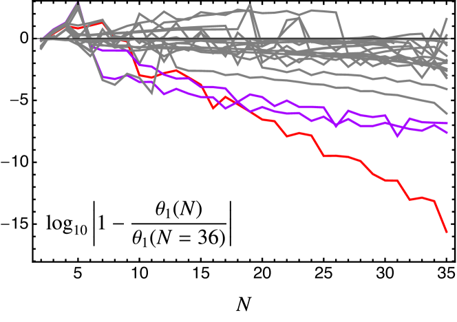
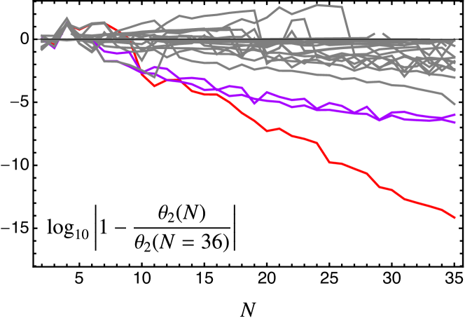
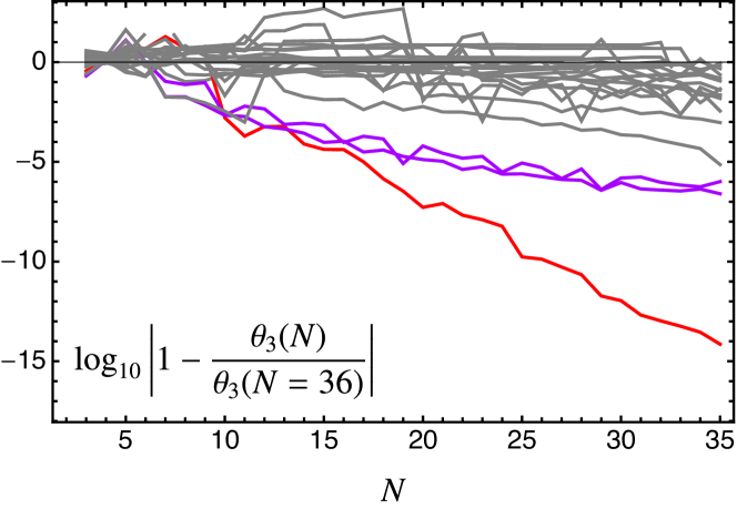
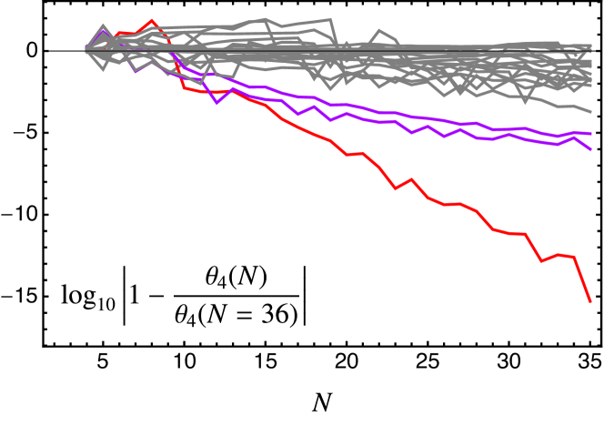
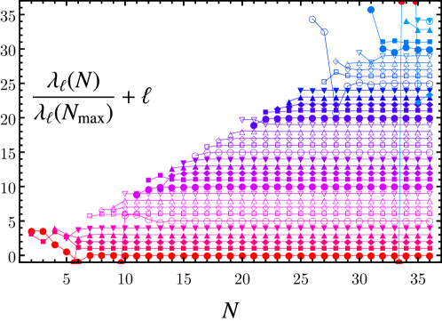
Once a fixed point candidate has been found consistently up to order , we further check its viability by studying convergence of couplings, and the stability and convergence of scaling exponents, and discard those which turn out to be unstable, have unnaturally large relevant or irrelevant eigenvalues, or show other inconsistencies. To explain this step, we show the convergence of the four most relevant eigenvalues for the fixed point candidates in Fig. 3.333Two spurious candidates have been excluded from the plot as they display unphysically large relevant eigenvalues of the order of (at ), and increasingly negative with increasing approximation orders thereafter. According to this figure, we select the three fixed points with the best observed convergence properties up to order . Note that some of the tertiary fixed points show a mild convergence in the first few scaling exponents which weakens, however, when going to higher orders. A similar picture is established in the convergence of fixed point coordinates. We emphasize that our criterion of convergence does not preselect the size of the gravitational scaling dimensions in any way.
This second step eliminates the 20 fixed point candidates termed ”tertiary”, including two fixed point candidates very close to the “secondary” ones which are not visible in Fig. 2. Hence, we are left with the primary Riemann fixed point and two secondary fixed points, highlighted by a red and a magenta arrow in Fig. 2. These fixed points are then computed to even higher approximations as discussed below. For ease of reference, we denote the three remaining fixed points as FP4s, FP4, and FP3, where the integer states the number of relevant eigendirections, and the subscript “” distinguishes the more strongly coupled fixed point of the two with four relevant directions. Occasionally, we also refer to FP4s as the “primary” Riemann fixed point whose properties are analysed in more depth in Secs. III and IV. The analysis and discussion of the secondary Riemann fixed points FP4 and FP3 is relegated to Sec.V.
A further consistency check of these fixed points found with standard boundary conditions is given by the use of non-perturbative boundary conditions as introduced in Falls:2014tra . Once a fixed point is found at all orders up to , the idea of improved boundary conditions at any lower approximation order is to fix the two highest couplings according to the values already found at the higher order approximations,
| (39) |
rather than (52). In (39), the barred couplings denote accurate estimates for the fixed point couplings deduced independently from a sufficiently higher order in the expansion, typically from an expansion up to with free boundary conditions (52). With this choice of boundary condition all fixed point couplings at approximation order automatically take the more accurate values of the fixed point couplings as determined from the highest approximation order . Besides stabilising the fixed point coordinates from the outset, the virtue of the a posteriori choice (39) is that it also leads to improved results for scaling exponents, most notably at low orders Falls:2014tra . For later reference, and opposed to (52), we refer to choices of the type (39) as improved boundary conditions.
III Riemann Fixed Point
We report in this section the evidence for the primary fixed point with Riemann tensor interactions and provide an overview of its main features such as coupling coordinates, convergence of effective action, de Sitter solutions and residuals.
A Fixed Point Coordinates
For the Riemann fixed point FP4s we have calculated its fixed point coordinates up to approximation order , involving up to powers of the Riemann tensor. We find that the fixed point coordinates fluctuate initially at low approximation orders, but then converge nicely starting with approximation orders . This is illustrated in Fig. 4 where we show the convergence of couplings, derived with standard boundary conditions and normalised to their asymptotic values at , up to approximation order . The pattern of convergence continues up to the maximal order (not shown).
Quantitative results are summarised in Tab. 2 for the first 14 fixed point couplings. The red-shaded areas indicate couplings which arise with the wrong sign at the leading order. Most of these adjust to the correct sign after a single step , except for or where the convergence requires 3 or 4 steps, respectively. Moreover, a fast convergence of couplings towards large is observed starting with approximation orders . Qualitatively, this is associated to the deviation of from its large limit in the first few approximation orders . Once has settled, all other couplings follow suit. The coupling proportional to the square of the Riemann tensor is expected to play a key role because it is canonically dimensionless. On the other hand, the initially slow convergence of at has no noticeable impact on the convergence of other couplings due to its smallness. Overall, we conclude that a viable Riemann fixed point has been identified which is very stable in the polynomial approximation.
Note, that the fixed point value for Newton’s coupling (Tab. 2) comes out nearly thrice as large as the result in the Einstein Hilbert approximation, in models, and in models, with all other technical parameters the same. Hence, this is an example where the higher order interactions impact noticeably onto the lower order fixed point couplings. A more detailed comparison is postponed until Sec. VII.
B Quantum Effective Action
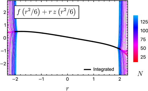
In Fig. 5 we show the fixed point effective action at the Riemann fixed point at different approximation orders . A converging behaviour within can be observed and it can be seen that the polynomial solution diverges alternatingly at the boundary of the converging regime. This suggests that the poles which limit the radius of the convergence of the polynomial solution are not on the real axis, but somewhere in the complex plane.
This behaviour and the fact that the fixed singularities of the differential equation (18) are at and suggest that the radius of convergence of the polynomial solution is not maximal and can be extended. It is then natural to numerically integrate the differential equation and enlarge the converging region. The result of the numerical integration is shown by the thick black line in Fig. 5. As expected, the radius of convergence is enlarged comparing to the polynomial case. The new radius of convergence reaches up to . More work is required in order to go beyond the point which necessitates the (numerical) lifting of an apparent pole in the flow; see Demmel:2015oqa ; Gonzalez-Martin:2017gza for examples.
We close with a general remark on global solutions. From the viewpoint of the asymptotic safety conjecture, it will be important to understand how the Reuter fixed point extends into a global fixed point, including the regime of asymptotically large fields. Using the method of functional renormalisation in simpler theories – such as or symmetric scalar theories or Gross-Neveu theories – global fixed point have indeed been found rigorously based on the invariants or , respectively. Identifying global solutions in gravity is more demanding, because many more independent invariants can be constructed out of the Riemann tensor. Further, it is not known which of these dominate the large-field asymptotics, nor whether the very same set will also dominate the small field region Falls:2018ylp . Therefore, it is not warranted to presuppose that global solutions must exist for any given subset of curvature invariants retained in the action.
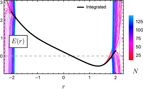
C Equations of Motion and de Sitter Solutions
Solutions to the equations of motion for quantum effective actions (32) evaluated on the sphere are of physical interest for inflationary cosmology as they correspond to Euclidean de-Sitter and anti de-Sitter solutions Baumann:2009ds ; Hindmarsh:2011hx ; Falls:2016wsa .444Note that this assumes the validity of analytic continuation to Lorentzian signature Falls:2016wsa . For recent discussions of subtleties related to the Wick rotation from Euclidean to Lorentzian quantum gravity, see Baldazzi:2018mtl ; Bonanno:2021squ ; Fehre:2021eob . Previously, de Sitter solutions have been found in the UV scaling regime of asymptotically safe and models of quantum gravity Bonanno:2010bt ; Falls:2014tra ; Falls:2017lst ; Falls:2018ylp .
Denoting the equation of motion as , we find for our model
| (40) |
Plugging in the couplings of the Riemann fixed point we can see how this equation behaves at different values for the dimensionless Ricci scalar. Using the polynomial approximation, this is shown at different orders in Fig. 6, where the first ten approximations have been neglected. Solutions to the quantum equations of motion obey . A first Euclidean de-Sitter solution is found at
| (41) |
Moreover, had we limited ourselves to just the Einstein Hilbert approximation, a de Sitter solution would be located at
| (42) |
Comparing (42) with (41) we observe a strong downward shift of the de Sitter solution due to the Riemann fixed point being more strongly interacting than the Einstein Hilbert one. Overall, the shift goes into the opposite direction as the shift induced by Ricci scalar or Ricci tensor interactions Falls:2016wsa ; Falls:2017lst ; Falls:2018ylp . Furthermore, if we take the Riemann fixed point and disregard all invariants beyond Einstein Hilbert (i.e. all Riemann interactions), the de Sitter solution (41) reduces to
| (43) |
Comparing (41) with (43) we conclude that the vacuum solution (41) arises primarily due to the fixed point value of the cosmological constant, while the set of higher order Riemann interaction terms has only a minor effect.
Further, approaches zero again just before the radius of convergence ends (Fig. 6). However, within the polynomial solution it is uncertain whether a second Euclidean de-Sitter solution is apparent at the fixed point or not. This question can be answered using numerical integration, which enhances the radius of convergence of the polynomial expansion and renders it maximal. In Fig. 6 we show the corresponding plot for the equation of motion. Indeed, the enlarged radius of convergence gives rise to a second Euclidean de-Sitter solution at
| (44) |
This vacuum solution is entirely due to higher order Riemann interactions and cannot be understood from within an Einstein Hilbert approximation. We conclude that the Riemann fixed point displays two dS solutions in the UV scaling regime. Further dS or AdS solutions may exist for larger positive or negative curvature, beyond the range studied here.
D Residuals and Absence of Poles
So far, we have considered the stability of couplings as well as the resulting effective action and de Sitter solutions of the Riemann fixed point FP4s. Now, we want to test the convergence of the fixed point as a polynomial solution of the flow equation.
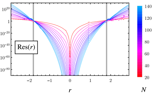
Firstly, in Fig. 7 we show the residuals of the flow equation (18) with (30), see also (34), at the Riemann fixed point,
| (45) |
It can be seen that the residuals shrink when more operators are included in the truncation, confirming the convergence of the fixed point solution. Further, the radius of convergence can be estimated to be . Note that the flow equation in (18) has fixed singularities at and coming from the zeros of . As we have discussed already, the fact that the radius of convergence of the polynomial solution is smaller than these fixed singularities suggests that it is not maximal.
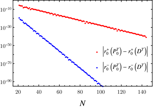
Apart from that, we observe small dips in the residuals of Fig. 7 at and . These features originate from removable singularities of the flow at the Riemann fixed point: At these points the denominator defined in Eq. (C.4) changes sign and has a zero. However, at the same time the corresponding numerator has a sign change and goes to zero as well, leaving the flow term finite, (C.3). In numerical approximations, however, these zeros are not at the exact same position. This leads to a spurious singularity responsible for the dips in Fig. 7. However, Fig. 8 shows that the differences between the zeros of the numerator and the denominator decrease strongly order by order at both points, and . This supports the view that the zeros of and are at the same position in the exact solution of the Riemann fixed point. This alone does not yet tell us that the singularity at those points is removable. However, we note that the derivative of the denominator converges to and at higher orders. Thus, we expect the derivative of the denominator to be non-vanishing at both and from which we conclude that the singularities are removable. Hence, we expect the full non-polynomial solution of the Riemann fixed point to be free of dips such as those in Fig. 7 and to be well-defined in the entire regime .
Finally, we use numerical integration to see whether the radius of convergence of the polynomial solution can be enhanced. To perform the numerical integration, we seek two differential equations for the highest derivatives of and . Starting from the flow equation, these can be obtained by splitting the flow into even and odd parts (in ) Falls:2017lst . In this way, we deduce a system of two coupled third order differential equations,
| (46) |
with . The functions and are rational functions depending only on and as well as their derivatives up to second order and explicit dependencies on .
In the form (46), we can integrate the fixed point equation and find the fixed point solution of and . As a consequence of the presence of spurious singularities for FP4s, however, this must be performed in patches. Otherwise, numerical uncertainties might lead to the numerical solution developing an artificial pole coming from a removable singularity. In practice, it is easiest to use the polynomial solution until we are beyond the removable singularity. This can also be motivated by the very small residuals of the polynomial solution for small , which are hard to achieve relying solely on a numerical integration. All in all, we use the polynomial expansion to provide the fixed point solution in the range , and further use these as initial conditions for the numerical integration starting at , with within . In this manner, we obtain a reliable fixed point solution over the maximal domain .
As an alternative method, we have also used Padé resummation to extend the polynomial solution. However, similar to Fig. 7 the residuals of Padé approximants can give rise to spikes. Such spikes originate from the removable singularities found in the polynomial approximation. As discussed above, we expect these singularities to be removable in the full solution. Within numerical precision, the result obtained from Padé resummation is in full agreement with the numerical integration and gives the maximal radius of convergence as seen in Fig. 5 and Fig. 6.
IV Universality and Critical Surface
In this section, we report our results for universal scaling exponents, the dimension of the UV critical surface, the set of fundamentally free parameters, and the bootstrap test for the Riemann fixed point. We also discuss the large order behaviour of scaling dimensions and signatures for weak coupling.
A Scaling Exponents and Infinite Limit
Universal scaling exponents describe how renormalisation group trajectories scale towards or away from interacting fixed points. In practice, they are deduced as the eigenvalues of the stability matrix . For each and every order of the approximation, we have computed the set of universal scaling exponents
| (47) |
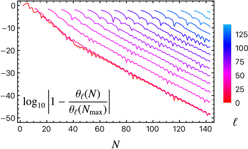
with eigenvalues sorted according to magnitude, and up to the maximal order . With increasing , we find that eigenvalues converge rapidly to their asymptotic values. This is illustrated in Fig. 9 which displays (minus) the number of relevant digits of scaling exponents which agree with the scaling exponents at the highest approximation order . By and large, the convergence is exponential with increasing . Roughly, enhancing approximation orders by leads to an additional significant digit in any of the scaling exponents.
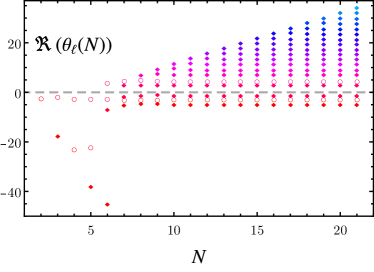
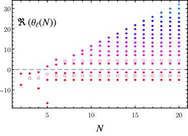
Using our results at the highest order and taking an average over the preceeding ten approximation orders we find an infinite estimate for the first seven scaling exponents
| (48) |
We have determined the leading relevant digits of these eigenvalues which have become independent of the approximation order, though for practical purposes, we only show the first six relevant digits. Hence, the errors of the calculated values are of order . Note that the error reflects the accuracy of the numerically determined fixed point solution. It does neither reflect truncation errors nor systematic errors. For strategies to access truncation and systematic errors within the functional RG framework, we refer to Litim:2010tt ; Litim:2000ci ; Litim:2001up ; Litim:2001fd . As such, however, the values (48) can be viewed as the infinite- limits for the various fixed point couplings. Note also that the canonical values of the four relevant eigenvalues are , , , and , see (26). Hence, the quantum corrections shift the real parts of the relevant eigenvalues by an amount of on average, pointing into the relevant direction for all of these eigenvalues (see also Sec. B).
We should also compare findings at the Riemann fixed point with those in the Einstein Hilbert approximation, where the scaling exponents are
| (49) |
For the first two scaling exponents, the real part of eigenvalues differ from classical values by and , respectively. Instead, the leading two exponents at the Riemann fixed point (48) differ from classical values by roughly one unit, and , respectively. Most notably, the exponent receives shifts into opposite directions. On the other hand, the exponent becomes more relevant due to quantum corrections in both cases. We conclude that quantum effects due to Riemann curvature invariants have a noticeable effect on the scaling exponents, both in view of classical or Einstein Hilbert exponents.
It is worth pointing out that the vast majority of eigenvalues are real rather than complex conjugate pairs. This is in contrast to approximations where about half of the eigenvalues are complex Falls:2014tra ; Falls:2016wsa , or -type approximations where most eigenvalues come in complex conjugate pairs Falls:2017lst . In the present case, only the second and third, and fifth and sixth most relevant eigenvalues turn out to be complex conjugate pairs while all other eigenvalues are real.
| Standard Boundary | ||||||
| Conditions | ||||||
| Improved Boundary | ||||||
| Conditions | ||||||
Next, we discuss the improved convergence of scaling exponents due to improved boundary conditions (see Sect. E). It has been shown previously that improved boundary conditions lead to an enhanced convergence of scaling exponents, in particular at low orders Falls:2014tra . Setting the boundary conditions according to the highest order fixed point couplings, fixed points will take the coordinates dictated by the highest order approximation, for all approximation orders, and the initial fluctuations as seen in Tab. 2 are avoided. Eigenvalues, however, change non-trivially under this choice of boundary conditions.
Results for eigenvalues are shown in Fig. 10 where we also compare standard and improved boundary conditions. In either case eigenvalues converge rapidly after . With standard boundary conditions (left panel) and smaller , couplings fluctuate strongly and large relevant eigenvalues arise. The appearance of spurious large negative eigenvalues at low orders has already been seen in earlier works Lauscher:2001ya ; Falls:2017lst ; Falls:2018ylp at . In contrast, with improved boundary conditions (right panel) the magnitudes of the large negative eigenvalues are substantially smaller. A quantitative comparison of eigenvalues is given in Tabs. 3 and 4. In Tab. 3 the first six eigenvalues of the Riemann fixed point are shown based on standard (upper) and improved (lower panel) boundary conditions. Red-shaded areas indicate if scaling exponents deviate by more than a factor of two from their asymptotic values. This affects many of the leading critical exponents from standard boundary condition including , , , and . In contrast, re-adjusting the underlying fixed point couplings to their asymptotic values via improved boundary conditions, we find that only the exponents are off by a factor . For example, the largest relevant eigenvalue at is reduced in magnitude from the unreliably large value down to by using improved boundary conditions. Most notably, the improved result at comes out very close to the exact result in the infinite- limit. Another feature of improved boundary conditions is that we now find a four-dimensional UV critical surface at , in accord with the result (48). In contrast, standard boundary conditions spuriously lead to a five dimensional UV critical surface.
| , | , | ||||
|---|---|---|---|---|---|
We conclude that the large fluctuations in the eigenvalue spectrum found with standard boundary conditions at low orders are significantly reduced using improved boundary conditions. At higher orders, starting at , eigenvalues from improved boundary conditions are already close to their asymptotic values (48), and only differ mildly from standard boundary conditions. Starting at , the significant digits in Tab. 3 no longer change with increasing and the differences in the boundary condition become irrelevant (Tab. 4).
B Dimensionality of UV Critical Surface
Another novel feature of the Riemann fixed point is its four dimensional UV-critical surface. As can be seen in Fig. 10, the fixed point has four negative and therefore relevant eigenvalues, one of which is a complex conjugate pair. The gravitational action (1) with (2) and (30) only includes two canonically relevant and one canonically marginal operator. Thus, we are led to the conclusion that quantum effects have turned a classically marginal and a classically irrelevant operator into relevant directions at the UV fixed point.
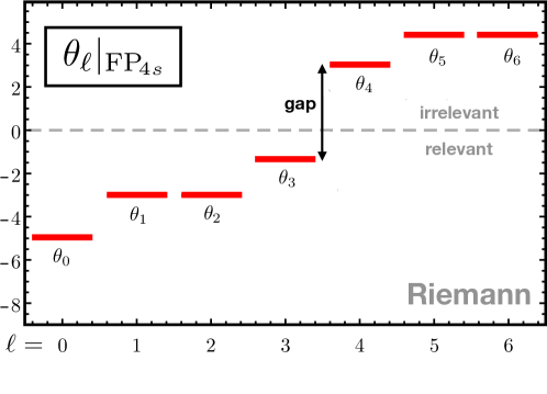
The UV critical surface is further illustrated in Fig. 11 where we show the seven most relevant eigenvalues for different approximation orders. We observe that eigenvalues (thin black lines) convergence rapidly to asymptotic values (red thick line), four of which settle at negative values. Of particular interest is the gap in the eigenvalue spectrum, corresponding to the difference between the largest relevant and the smallest irrelevant scaling exponents. In the free theory, this gap is . At the interacting fixed point, the most irrelevant of the relevant eigenvalues is and the most relevant of the irrelevant eigenvalues is . Their gap is given by
| (50) |
We observe that the gap is larger than the classical gap. However, it is smaller than the gap in theories Falls:2014tra ; Falls:2018ylp and smaller than the gap in theories with Ricci tensor interactions Falls:2017lst . The difference originates from the fact that the quantum effects make the first classically irrelevant eigenvalue more relevant quantum-mechanically in the present case, leading to a smaller gap and to the ordering .
C Fundamentally Free Parameters
It is interesting to discuss the set of fundamentally free parameters from the viewpoint of the full quantum theory of gravity Falls:2018ylp . The family of quantum gravity models (1), (2) always contains the Einstein-Hilbert interaction terms and . For both of these classically relevant interactions, the corresponding couplings are found to be relevant in the quantum theory, giving the Reuter fixed point Reuter:1996cp ; Souma:1999at ; Litim:2003vp . On the level of fourth order interactions, our models retain any one of the invariants
| (51) |
or a linear combination thereof. We recall that the invariants (51) cannot be distinguished within projections on maximally symmetric spaces (adopted here). Nevertheless, for either of these classically marginal interactions, it is found that the corresponding coupling becomes relevant in the quantum theory Falls:2013bv ; Falls:2014tra ; Falls:2017lst . This is in accord with the lower bound
| (52) |
on the number of fundamentally free parameters Falls:2018ylp . Based on fourth order extensions of gravity, and neglecting the potential impact of higher order curvature invariants, similar conclusion have been reached in Benedetti:2009rx ; Niedermaier:2009zz ; Falls:2020qhj . An important new observation of this work arises for dim-6 invariants. Of these, our models (1), (2) can retain any one of the invariants
| (53) |
or any linear combination thereof. In models which retain the term with Ricci scalar or Ricci tensor interactions, no new relevant direction is created and we are left with (52). In contrast, for models with Riemann interactions, (31), (32), a new relevant eigendirection can be found. In other words, the dynamics of Riemann tensor interactions displays qualitative differences from Ricci scalar or Ricci tensor interactions starting at dim-6. A discussion of the corresponding eigenperturbations is relegated to Sec. C below.
A conservative interpretation of this result for the full theory of quantum gravity is that at least one of the canonically irrelevant dim-6 invariants (see Tab. 1 for an overview) becomes a relevant operator due to quantum fluctuations. This does require quantum corrections to scaling dimensions to be of order unity, which has previously been observed in many asymptotically safe models. What is new here is that the quantum corrections make the dim-6 interaction more relevant rather than more irrelevant. In consequence, it indicates that the UV theory of pure quantum gravity has at least
| (54) |
fundamentally free parameters. In order to further clarify the number of free parameters, it will be important to investigate other dim-6 invariants in future works (Tab. 1) including the Goroff-Sagnotti term Goroff:1985sz ; Goroff:1985th ; Gies:2016con , while also retaining sufficiently many higher dimensional interaction terms for eigenvalue spectra to become reliable.
D Bootstrap and Large Order Behaviour
The bootstrap approach to quantum gravity is a systematic way of testing whether a fixed point candidate is viable or otherwise Falls:2013bv . The fundamental assumption is that canonical power counting remains to be a good ordering principle for operators even at an interacting fixed point, which is known to hold true for fixed points observed in nature. A virtue of the bootstrap hypothesis is that it can be confirmed a posteriori. Specifically, starting at some approximation with different operators, the eigenvalue introduced by a new operator of higher mass dimension should turn out to be more irrelevant than other eigenvalues. Further, the eigenvalues already included in the truncation before should only change by small fluctuations. In particular, from a sufficiently high order onwards, new relevant eigenvalues should not be created. To test this conjecture for the Riemann fixed point, we take a look at the quantity
| (55) |
This quantity gives the largest eigenvalue in the eigenvalue spectrum at approximation order . For the bootstrap to be viable, we expect that the functions are growing with increasing , which manifests that the addition of a new high-order invariant in the step from leads to a new eigenvalue which is less relevant than those identified in previous approximations. This pattern also ensures that no new relevant eigenvalues are created when higher operators are included. In Fig. 12 we see that this is clearly the case for the Riemann fixed point as soon as or larger, in agreement with the bootstrap conjecture, which verifies our working hypothesis.
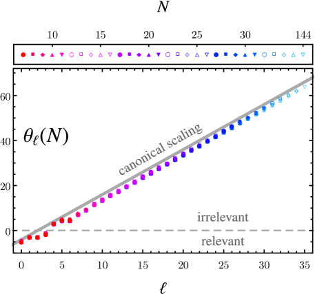
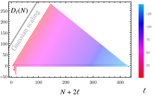
Having seen that the bootstrap approach is fulfilled for the Riemann fixed point we want to further investigate the eigenvalue spectrum. In particular we are interested to ask how far away the observed eigenvalues are from Gaussian scaling. For that purpose, Fig. 13 shows the eigenvalues obtained at different orders in comparison with their Gaussian values (26),
| (56) |
indicated by a grey line. As can be seen, eigenvalues are close to their Gaussian values with small deviations due to quantum corrections. This is in accordance with other works Falls:2018ylp ; Falls:2017lst ; Falls:2014tra ; Codello:2008vh where eigenvalues are observed to be “as Gaussian as it gets”. A difference to these works is that quantum corrections are strictly shifting eigenvalues towards relevant directions, leading to, among other, the observed four dimensional UV critical surface. It is also worth noting that the largest corrections towards relevant directions are received by the eigenvalues with and as seen by the dips in Fig. 13. The largest correction, at , is given by
| (57) |
We further investigate the deviations from Gaussian scaling in Fig. 14 where the difference between the real part of the eigenvalues and their canonical counterparts in (56) at different orders is shown. As we see, the quantum corrections to scaling are of the order of for all eigenvalues, which substantiates the observation that, except for the leading few, most of the quantum gravitational scaling dimensions are near-Gaussian with only small relative deviations.
More precisely, the first ten eigenvalues follow rather stochastic fluctuations around Gaussian scaling while higher eigenvalues show very systematic deviations: Eigenvalues with enter relatively close to Gaussian scaling when they are included for the first time and then drift away to their final value when the truncation order is increased and more operators are included. Furthermore, the line of final values for the deviation is bended in Fig. 14, showing that higher eigenvalues are getting closer to Gaussian scaling.
The mean deviation of the first ten eigenvalues from Gaussian scaling at order , , is given by
| (58) |
and points into the relevant direction. This deviation is of the order of three within one standard deviation. Returning to our assumption that only eigenvalues corresponding to operators from Tab. 1 should become relevant in the UV, we see that the observed shift can indeed be big enough to do so. The Riemann fixed point FP4s is a particular example for this to happen.
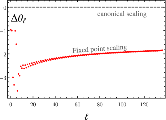
Moreover, we note that within our setup a shift of in the relevant direction for the low eigenvalues is only away. Hence, our observations in the eigenvalue spectrum do not rule out the possibility of rendering an eigenvalue corresponding to a dim-8 operator relevant. How likely it is for an eigenvalue of a dim-8 operator to become relevant is hard to estimate from our analysis, since the offset from Gaussian scaling and its standard deviation changes between settings and approximations. However, it is clear that we should not rule out the possibility of eigenvalues corresponding to dim-8 operator becoming relevant at an interacting fixed point for gravity.
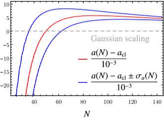
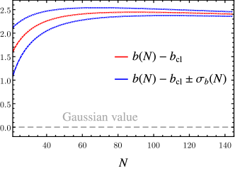
The pattern in the deviations of higher eigenvalues from Gaussian scaling in Fig. 14 suggests that there might be a simple linear relation between these higher eigenvalues. Therefore, we use the results obtained at different orders and fit a linear function to the eigenvalue spectrum. Since the last eigenvalues of every approximation need a few more orders to settle to their final values, we exclude the last ten eigenvalues of each order from the fit. Then, fitting the linear function
| (59) |
we obtain the results shown in Fig. 15 for different approximations starting from up to . At the highest approximation, we find
| (60) |
According to (56) the Gaussian values for these parameters are given by
| (61) |
Hence, the fitted slope of the Riemann fixed point is very close to Gaussian scaling. The y-intercept (, on the other hand, is shifted away from its Gaussian value by an amount of . This is roughly the same amount as the observed average shift in the first ten eigenvalues of the spectrum (58).
To summarise, we find that the eigenvalues of the Riemann fixed point follow near-Gaussian scaling with quantum induced shifts. These shifts in effective mass dimension are such that operators invariably become more relevant. The magnitude of shifts is of the order of . Note that this is different from what has been found in models of gravity where quantum corrections mostly shift eigenvalues into irrelevant directions. Hence, we come to the conclusion that the dynamics induced by the Riemann tensor interactions included in settings of the form (32) are distinct from those found for a -type models, or of models involving Ricci tensor interactions such as (1) with (2) and . In particular, this manifests itself in generating a four dimensional UV critical surface for the Riemann fixed point.
E Signatures of Weak Coupling
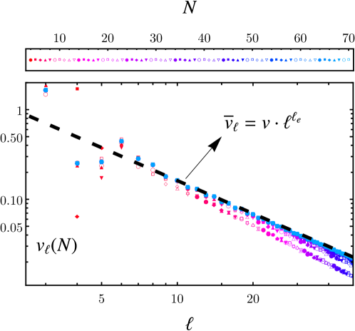
The near-Gaussian behaviour as observed above can be further discussed. For that purpose, we define the quantity which measures the relative deviation of scaling dimensions from classical values,
| (62) |
Here denotes classical eigenvalues and are observed eigenvalues at different approximation orders . Fig. 16 shows this quantity in a double logarithmic plot for orders up to and eigenvalues up to . As we see, the plot shows a linear relation between the quantities and . This suggests a functional relation of the form
| (63) |
Fitting this function to the observed eigenvalues at highest order with the last ten eigenvalues being excluded gives and . Fig. 16 shows that this relationship with these values is fulfilled to a good approximation. This can also be confirmed to higher orders which are not shown here for illustrative reasons. If this functional dependence remains to be true at higher orders the quantity will approach zero for high eigenvalues. This means that higher eigenvalues are getting closer and closer to their canonical values and eventually end up there. Thus, the induced quantum corrections to scaling exponents become smaller for higher eigenvalues which gives another notion of the term “as Gaussian as it gets”. Moreover, it can be interpreted as a signature of a hidden weak coupling controlling Gaussian scaling of higher operators.
It is worth pointing out that the approach to Gaussian values is algebraic, and much slower than the approach observed in truncations involving Ricci scalar or Ricci tensor interactions. Specifically, for actions or actions of the form the Gaussian approach have been found out to be exponential and therefore faster than the observed power law behaviour in the truncation. However, in the case of only different approximation orders have been taken into account. Also, approximations tend to have stronger fluctuations in couplings and eigenvalues. Thus, our results are somewhat more precise in that matter.
V Weakly Interacting Riemann Fixed Points
In Fig. 2, we have pointed out that our fixed point search gives rise to three candidates which pass the viability tests and which do not suffer from unnaturally large relevant/irrelevant eigenvalues or strong instabilities in eigenvalues. In this section, we discuss our results for the two secondary, weakly interacting Riemann fixed points FP4 and FP3 (magenta dots in Fig. 2). should not be confused with the primary Riemann fixed point (FP4s) of the previous sections.
A Fixed Point Coordinates
Within the polynomial expansion, the coordinates of the secondary fixed points and fluctuate at low orders but stabilise thereafter. This is not unexpected, and very similar to what has been observed for the primary Riemann fixed point. The fixed point coordinates of stabilise around the order . We notice that its couplings are very close to those of . In this light, we may interpret this as the fixed point splitting up into two fixed points and starting from order onwards. After these orders both fixed points are stable and arise consistently at each and every order, up to the highest orders.
Quantitatively, the first couplings of the fixed point effective action (32) at are
| (64) | ||||
To achieve these, we have used a polynomial expansion of the action (1) with (31) and using (33) up to the order . In terms of the couplings (27) we have
| (65) |
Clearly, the values (65) are close to those of the Einstein Hilbert approximation (38), see Fig. 2. This data should be compared with the first few couplings of , for which we find
| (66) | ||||
To achieve these, we have used a polynomial expansion of the action (1) with (31) and using (33) up to the order . We notice that the first three couplings at FP3 (66) are close to those at FP4 (64). The first coupling which differs substantially is . In terms of the couplings (27) we find
| (67) |
which, again, comes out quite close to the Einstein-Hilbert result (38). The vicinity of (65) and (67) to (38) allows to interpret these fixed points as higher order extensions of the Reuter fixed point.
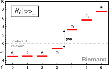
B Scaling Exponents and Critical Surface
For both and we have computed scaling exponents up to very high order in the polynomial expansion. In either case, we found that the scaling exponents satisfy the bootstrap test as performed for the Riemann fixed point in Sec. D. Moreover, we have also confirmed that large order scaling exponents for and become near-Gaussian, in full analogy with the Riemann fixed point and earlier findings for and type theories. Quantitatively, the first few scaling exponents at read
| (68) | ||||
Several comments are in order. Firstly, we notice that the critical surface is four-dimensional, similar to what has been found at the Riemann fixed point (48). Quantitatively, three of the four relevant exponents are close to those at the Riemann fixed point, with , except the leading one which differs more substantially, . On the other hand, the gap in the eigenvalue spectrum (68) is given by
| (69) |
and is very close to, if mildly larger than, the Riemann gap (50). In comparison with the Einstein Hilbert approximation (49), the two leading exponents in (68) are more relevant, with . We conclude that quantum effects due to Riemann curvature invariants make the fixed point more relevant compared to the Einstein Hilbert approximation, and despite of the fact that the two leading couplings remain essentially unchanged.
Comparing the scaling exponents of with classical values, we find that the real part of the first two scaling exponents differ from classical ones by and , respectively. This can be compared with the shifts of and induced by the Einstein Hilbert approximation alone. In both cases, the leading exponent receives shifts towards positive values, while the second most relevant exponent receives negative quantum corrections. Moreover, all higher order Riemann tensor interactions together make the leading scaling exponents and more relevant by and units compared to the Einstein-Hilbert ones.
Let us now discuss the large-order behaviour of universal eigenvalues in more detail by performing a linear fit as in (59). Overall, we find a pattern similar to the one observed in Fig. 15 for the Riemann fixed point. Due to a slowed-down convergence of eigenvalues (to be discussed in Sect. D) we take the average of values for the slope and the offset parameter over the ten highest approximation orders to find
| (70) |
Similar to what is found at the Riemann fixed point (60), the slope is very close to its Gaussian value (61). The shift in the offset is pushing the eigenvalues into the relevant direction and comes out much smaller than at the Riemann fixed point (Fig. 15).
It is well-known that the Einstein-Hilbert fixed point and fixed points are connected with the Gaussian fixed point of classical GR by well-defined RG trajectories. Given that is numerically close to the Einstein-Hilbert and values of the leading two fixed point couplings, it is conceivable that RG trajectories should exist which flow from in the UV to classical GR in the infrared (see Sec. C). Indeed, we have checked by numerical integration that a weakly coupled low energy regime with (29) and the emergence of General Relativity is realised from the UV fixed point.
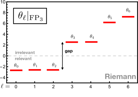
For the fixed point, we find the scaling exponents
| (71) | ||||
The critical surface is three-dimensional, similar to what has previously been found at the and fixed points. Quantitatively, the three relevant exponents are close to the leading three exponents at the fixed point, and less relevant with . On the other hand, the gap in the eigenvalue spectrum (71) is given by
| (72) |
and is larger than the Riemann gap (50), and larger than the gap at the fixed point (69). We also notice that the gap is much closer to the gap observed in theories, yet still much smaller than found for theories with three relevant couplings.
Let us now compare exponents with classical and Einstein Hilbert values. For the first two scaling exponents and , the real part of eigenvalues differ from classical values by and , respectively. This should be compared with the shifts by and in the EH approximation, (49). Hence, not only are the fixed point couplings at very close to those of the EH approximation, but the quantum corrections of the two leading exponents are similarly close to those already induced when only the two leading operators are retained. In other words, at the quantum effects due to all curvature invariants with canonical mass dimension and higher (all invariants beyond the cosmological constant and the Ricci scalar) only contribute the shift and to the two leading exponents, which furthermore is half as large as the shifts at . Once more, Riemann tensor interactions make the scaling exponents more relevant, albeit mildly. It is in this sense that is as close as it gets to the Reuter fixed point.
Turning to the large-order behaviour of universal eigenvalues we perform a linear fit as in (59). We again find a pattern similar to the one observed in Fig. 15 for the Riemann fixed point. Taking the average of values for the slope and the offset over the ten highest approximation orders we find the estimates
| (73) |
We notice that the slope parameter is essentially classical with in accord with the approach to near-Gaussian scaling. Also, the shift is smaller then what is found at (70) and at the Riemann fixed point (60). These findings further underline that this fixed point is as close to the Reuter fixed point as it gets.
C Effective Action and de Sitter Solutions
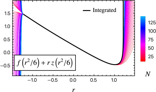
Next, we discuss the curvature dependence of the weakly interacting Riemann fixed points. In Fig. 19 we show the fixed point functional at the fixed point for different orders as a function of dimensionless curvature . We observe that the polynomial approximation shows an alternating-sign convergence on the negative real axis and a same-sign convergence on the positive real axis. The latter is often indicative for the presence of a pole. We confirm this view by a full numerical integration of (19) at the fixed point, which is unproblematic due to the absence of removable singularities. Hence, it appears that the fixed point solution does not extend beyond dimensionless background curvatures of order unity in the present approximation.555Due to this divergence we can neither continue the integration on the negative nor on the positive side in Fig. 19. This is due to how the differential equations are integrated using two functions and depending on the square of the Ricci scalar curvature. Each function on its own is independent of the sign of the scalar curvature and takes the same value for positive and negative curvature. Only the sum of them which enters the effective action may differ on the positive and the negative side. It is interesting to note that this pole is not generated by a pole in the differential equation. Instead, it is of the Landau type and generated dynamically similarly to Landau poles in perturbative -functions, e.g. QED. Since we expect the fixed point functional to be well-behaved for all dimensionless Ricci scalar, this result suggests that possibly new effects must arise due to further curvature invariants which ensure that the effective action extends to larger curvature (recall that our study employs the heat kernel expansion which is well-suited for small curvature). Similar results and conclusions apply for the fixed point .
Next, we search for de Sitter solutions in the deep UV. With increasing curvature, the fixed point functionals essentially behave linearly up to the end of the radius of convergence, see Fig. 19. This behaviour, together with the proximity of the fixed point couplings to EH values, suggests that the equations of motion will have de Sitter solutions similar to those of the Einstein-Hilbert approximation. Quantitatively, we find one de-Sitter solution for each of the fixed points and . Their numerical values are given by
| (74) |
respectively. Both are larger than the EH result (42), and all three are larger than the de Sitter solution (41) of the strongly interacting Riemann fixed point. Retaining only the cosmological constant and the Ricci scalar terms of the fixed point action, the result would have come out as and . Here we used (65), (67), and the fact that in any Einstein-Hilbert theory. The result strengthens the view that the and fixed points are weakly coupled, and only differ mildly from the Reuter fixed point.
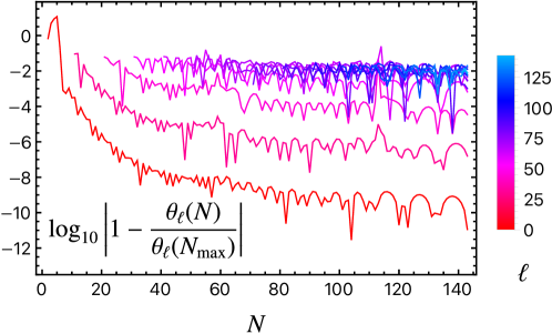
D Convergence
In Fig. 20, we show the convergence of eigenvalues towards their values at approximation order . For the Riemann fixed point, all eigenvalues converge algebraically fast (Fig. 9). However, this is not observed for . Rather, a fast and constant rate of convergence is observed for the first 20 orders in the expansion, reaching up to six significant digits in the exponents. With increasing order, however, the rate begins to flatten and the accuracy stops increasing around the order . Specifically, the findings show that the scaling exponent cannot be determined beyond an accuracy of , and increasingly less so for the higher order eigenvalues. A similar behaviour is found for the fixed point couplings of the weakly Riemann fixed points and , and for the scaling exponents of the fixed point .
The slight deterioration of convergence towards the highest orders is further corroborated in Fig. 21, where we show the difference of the real part of the eigenvalues and their classical scaling at different orders . This should be compared with the result at the Riemann fixed point (see Fig. 14). Overall, eigenvalues approach Gaussian values with small deviations, as seen for the Riemann fixed point. However, in contrast to Fig. 14, this plot shows that the convergence of increasingly irrelevant eigenvalues slowly deteriorates. While up to an apparent convergence of eigenvalues can be seen, higher eigenvalues continue to strongly fluctuate within a belt around Gaussian scaling, another consequence of the lack of convergence at highest orders (see Fig. 20). Similar results are found for . In summary, we are lead to the conclusion that a full determination of the fixed point and its scaling exponents cannot be achieved beyond a limiting accuracy within the local curvature expansion of the effective action performed here. However, since the effect is numerically small, and most likely below systematic errors due to approximations, it may be neglected for the present purposes.
It is conceivable that the slight lack of convergence is a technical artifact, which can be overcome by an extended study using different momentum cutoffs, or by using spectral sums instead of heat kernel expansions. In functional RG studies of critical phenomena it has been noted that certain technical choices may hamper the accurate determination of scaling exponents due to convergence-limiting poles in the complex plane Morris:1994ki . Still, the apparent lack of convergence can be overcome by taking constant field backgrounds Aoki:1998um ; Litim:2001dt , by using more suitable cutoffs Litim:2002cf , or by dropping the polynomial approximation in the first place Morris:1994ki . These extensions, albeit interesting, are beyond the scope of the present work.
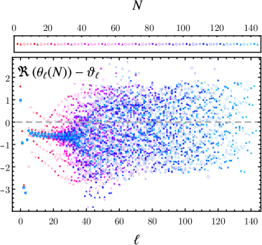
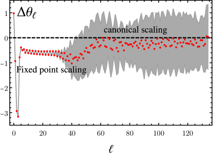
VI Eigenvectors and Equal Weight Condition
In this section, we summarise results for eigenvectors and eigenperturbations. As a main novelty we put forward an “equal weight” condition which allows the identification of eigenperturbations irrespective of overall parametrisation ambiguities of couplings in the effective action.
A Eigenvectors
The goal of analysing eigenvectors is to clarify which invariants in the effective action relate to which eigenvalues, and to understand which interaction monomials dominate the relevant eigendirections. We expect that there will not be a one-to-one correspondence between an eigenvector and monomials in the effective action. Rather, different operators in the effective action mix and as a result eigenvectors often do not point into the direction of an individual monomial only.
To begin with, we define the eigensystem of eigenvalues and eigenvectors at approximation order via the stability matrix at the fixed point, ,
| (75) |
where we use to label different eigenvalues and their corresponding eigenvectors . Having calculated this eigensystem for the Riemann fixed point at different orders, we plot the absolute values of the components for eigenvectors at and in Fig. 22. Starting with a discussion of the eigenvectors at , we observe that all eigenvectors appear to be dominated by classically irrelevant interactions: The largest components of all eigenvectors point into the directions of the five highest included operators in the truncation. In contrast to this, other directions corresponding to operators with smaller mass dimension are suppressed in all eigenvectors. However, taking a closer look we see that the components corresponding to operators of small mass dimension are significantly enhanced in the relevant eigenvectors. Moreover, the most irrelevant eigenvectors only get significant contributions from the classically most irrelevant eigenvectors in the truncation.
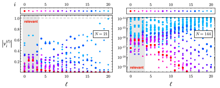
Qualitatively similar features can be seen in the eigenspectrum at as well. Again, the whole eigenspectrum appears to be dominated by the classically most irrelevant directions included in the truncation. In particular, relevant eigenvectors are dominated by the highest operators included in the truncation and classically relevant directions contribute significantly more to relevant eigenvectors than irrelevant ones. However, note that the quantitative values have changed drastically by going from to . While the classically relevant directions had contributions of the order of in the first case, these contributions are suppressed to orders of in the latter. Further, all operators which are included at turn out to be strongly suppressed by higher operators which are additionally included at .
Some of the features seen in Fig. 22 are reasonable ( the fact that classically relevant directions contribute significantly more into the directions of relevant eigenvectors) but others are clearly not ( the fact that all eigenvectors seem to be dominated by the classically most irrelevant operators). Moreover, the findings do not reflect the order-by-order stability of fixed point couplings and eigenvalues.
B Equal Weight Condition
We are now going to make the case that the eigenvectors in Fig. 22 do not display universal features of the theory, while a suitably modified version of them does. To appreciate this point we note that eigenvectors, unlike eigenvalues, are not universal quantities in the sense that they change under a redefinition or rescaling of the underlying fields or couplings. For example, if we rescale polynomial couplings as (no sum), the corresponding -functions are given by . It then follows that the elements of the stability matrix of the rescaled system are given by
| (76) |
While eigenvalues remain unchanged, eigenvectors do change, as can be seen from the relationship between eigenvectors before and after rescaling,
| (77) |
In general, the normalisation of an eigenvector changes under rescaling of couplings, and we may introduce rescaled eigenvectors, normalised to unity, as
| (78) |
A remnant of this ”rescaling ambiguity” is visible in Fig. 22, where the entire eigenspectrum appears to be dominated by the highest operators retained in the approximation. As is evident from (77) with suitable choices for the rescaling parameters any operator can be made to appear dominating the eigenspectrum.
To remedy this ambiguity, we lay out a simple procedure to find eigenvectors which are best qualified to describe the physical eigenperturbations without any rescaling ambiguities. Since we are only interested in the physical information of the eigensystem, we fix the rescaling ambiguity such that all operators contribute with ”equal weight” to the entire eigensystem. This idea ensures that no operator is dominating artificially in the spectrum, and should leave us directly with the physical information stored in the eigenvectors. On a quantitative level, this amounts to the ”equal weight” condition for the rescaling parameters ,
| (79) |
Note that this equation sums over different vectors with the components held fixed. In physical terms, the condition (79) imposes that the absolute-value-squared contributions of any operator to all eigenvectors adds up to unity. In this manner, it is guaranteed that the contributions to eigenvectors of all operators retained in the approximation are weighted equally.
In addition, recall that the are defined such that they also fulfil the conventional ”unit length” normalisation condition for eigenvectors,
| (80) |
which sums over different components . Thus, considering the matrix of eigenvectors,
| (81) |
the normalisation conditions (79) and (80) correspond to normalising the absolute-value-squared sum of each row and each column to unity.
Next, we show that the equal weight (79) and unit length condition (80) for the matrix (81) can always be achieved. The condition (80) follows trivially from the normalisability of eigenvectors. The condition (79), on the other hand, requires a special choice for the rescaling parameters , which can always be achieved. To see this, we write (79) in terms of (78) to get
| (82) |
Notice that due to the normalisation of eigenvectors, an overall rescaling factor,
| (83) |
drops out of (82) leaving us with only open parameters. Due to the irrelevancy of this overall factor, we can always choose the rescaling factors to be of the form
| (84) |
With this choice, we can use the open parameters of (84) to fulfil (82) for all . Doing so, in the matrix of eigenvectors (81) this corresponds to having all columns and all rows except for the first row normalised to . From this it follows, however, that
| (85) |
Thus, fulfilling (82) for and normalising all eigenvectors automatically ensures that (82) is fulfilled for as well. It is, therefore, always possible to rescale the eigenvectors such that the naturalness condition (79) is fulfilled.
C Eigenvectors from Riemann Interactions
In Fig. 23, we apply our procedure to the theory at hand and show eigenvectors rescaled according to (79) and (80), and for different truncation orders and . We emphasise that our procedure has been applied to the full eigenspectrum at order and , even though only the first eigenvectors are shown in either case. The results in Fig. 23 should now be compared with Fig. 22, where several points are worth noting. First, with the equal weight normalisation, eigenvectors are now seen to be stable from order to order in the approximation, including up to the highest order. This is consistent with the order-by-order stability of fixed points and eigenvalues, but much unlike the pattern observed in Fig. 22. Second, we observe that eigenvectors associated to the relevant eigenvalues are dominated by linear combinations of the leading few operators with small mass dimensions. The result reflects the fact that interactions induce strong correlations amongst the leading few interaction terms, implying that linear combinations of them scale with identical exponents (see Tab. 3). Third, we also observe that increasingly irrelevant eigenvalues become dominated by a single interaction monomial with canonical mass dimension , with other monomials only providing subleading corrections. This result reflects the near-Gaussian scaling of operators with increasing mass dimension observed in the previous section (Sect. D). We conclude that key features of the eigensystem have become visible thanks to a suitable normalisation of eigenvectors.
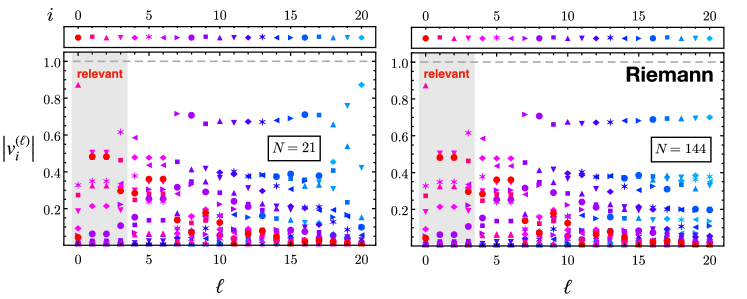
We may now take a closer look at Fig. 23 to understand which interaction terms are responsible for the four-dimensionality of the UV critical surface. To that end, we divide the set of eigenvectors into subsets of strongly and weakly correlated eigenvectors. The set of weakly correlated eigenvectors contains those where each eigenvector is approximately dominated by a single operator in the effective action. If so, it means that quantum corrections are small, only introducing mild mixing, and a rough correspondence between eigenvectors and field monomials can be established. On the other hand, the set of strongly correlated eigenvectors are those which show a strong mixing between interaction monomials. Here, quantum effects are strong, and an association of an eigendirection with a unique interaction monomial is no longer possible.
In Fig. 23, the first subset contains the eigenvectors with while the second one consists of those with . Specifically, the vacuum energy contribution to the most relevant eigenvector is suppressed, despite of being the operator of lowest canonical mass dimension in the effective action. Rather, the eigenvector is dominated by the classically marginal operator , modulo corrections from other leading interaction terms. Similarly, the complex conjugate pair of eigenvalues corresponding to and have leading contributions from the vacuum energy and the interaction, while gets its largest contribution from the interaction which, classically, is irrelevant with eigenvalue . Hence, the naive expectation that the four most relevant eigenvectors correspond to the four classically most relevant operators does not hold true. Rather, all eigenvectors in the first part of the plot (all eigenvectors with ) get contributions due to mixing, which, moreover, can be large quantitatively. We conclude that the interaction terms responsible for the four-dimensional UV critical surface are not only the four classically most relevant operators. Rather, the mixing between operators up to and including is responsible for the four relevant eigenvalues. This matches the observation that the fixed point converges poorly (with standard boundary conditions) at low approximation orders up to and including (see Tab. 3), which is now understood as a remnant of strong correlations amongst eigenperturbations.
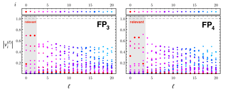
The same analysis of eigenvectors can now be done for the secondary fixed points and . Without using the equal weight condition, the resulting plots show qualitatively the same picture as Fig. 22 for the primary fixed point: The ad hoc eigenvectors spuriously appear to be dominated by the canonically most irrelevant operators in the spectrum with the canonically most relevant operators being enhanced in the relevant directions.
Using the equal weight condition, on the other hand, a stable and transparent picture becomes visible. Our results are shown in Fig. 24 where the first eigenvectors calculated at the highest approximation order ( for , and for ) are shown. In either case, the relevant eigenvectors (grey shaded area) are dominated by leading operators of small mass dimension – the cosmological constant, the Ricci scalar, and the interaction. For , we also notice that the operator contributes sizeably to the relevant eigenvectors. In turn, irrelevant eigenvectors are dominated by canonically irrelevant operators. In comparison with the primary fixed points Fig. 23 we note that the mixing between different operators in relevant directions is smaller. This is balanced by a stronger mixing of operators in the irrelevant eigenvectors. The one-to-one correspondence observed earlier is much weaker and there is a shift between irrelevant eigenvectors and their corresponding operators. Due to the weaker mixing in relevant directions, the correspondence between relevant directions and operators is clearer and we expect that the relevant directions are created by the operators up to and including . In comparison with the primary fixed point, the canonically marginal interaction now contributes much less to the leading eigenvalue. The three most relevant directions have eigenvalues of roughly the same magnitude and arise from linear combinations of the cosmological constant, the Ricci scalar and the interactions. For all three of these fixed points, it can be seen that the second and third most relevant eigenvectors get substantially large contributions from the cosmological constant.
We also observe from Fig. 24 that the increasingly irrelevant eigenvectors are approximately dominated by the interaction monomial for even and by terms for odd , with in the range covered by Fig. 24. The shift increases further with increasing beyond . This observation applies to both and , with other monomials only adding subleading corrections. The result indicates, once more, that the UV scaling of higher curvature interactions is non-classical despite of being near-Gaussian.
VII Discussion
In this section, we compare our results from Riemann tensor interactions with earlier higher order studies involving Ricci scalar and Ricci tensor interactions. We also discuss the impact of higher order curvature invariants on fixed point couplings and a scale invariant notion for the interaction strength, and on vacuum solutions to the quantum equations of motion.
A Ricci vs Riemann Interactions
We begin with a comparison of results of -type actions studied in this work with results from and actions, summarised in Tab. 5. A first important joint feature is the near-Gaussianity of high order eigenvalues in all three settings. Even though other aspects differ from each other, the near-Gaussian scaling of the eigenvalues seems to be hard-wired in all of them. This can be seen as an indication that the gravitational fixed point shows signatures of weak couplings as the classical eigenvalues are only corrected by small quantum corrections, especially regarding high eigenvalues. Since this feature is present in all three settings we have reason to believe that only a finite number of eigenvalues will become relevant at an interacting gravitational fixed point as the quantum corrections are not expected to be big enough to render arbitrary classically irrelevant eigenvalues relevant.
Apart from this feature, the and fixed points show further similarities. After initial fluctuations at low approximation orders both truncations show a fast convergence in the fixed point couplings and eigenvalues. The radius of polynomial convergence is maximal in the case and almost maximal for the polynomial solution of . In the latter setting, however, it becomes maximal using Padé resummation or numerical integration. Further, both settings have two de Sitter solutions. The AdS solution apparent in is, however, missing in . In contrast, -type theories are different in these aspects. The polynomial radius of convergence is only half of the maximal possible radius, and the convergence of couplings and eigenvalues is rather slow. dS and AdS solutions can both be found in quantum gravity.
Further differences appear in the spectra of eigenperturbations. Most notably, we have indications that operators including the square of the Riemann tensor induce a relevant fourth direction to the UV critical surface. This is a very important novelty, hinting at the relevancy of Riemann tensor interactions. Moreover, we also observe that only two pairs of eigenvalues in -type theories arise as complex conjugates (Fig. 10). This is quite different from and -type models where complex conjugate pairs continue to arise with increasing approximation orders. In general, complex scaling exponents indicate a degeneracy Falls:2014tra , meaning that the RG scaling of two sets of eigenoperators has become identical up to a phase. Including more interaction terms should lift the degeneracy, and eigenvalues in the full physical theory are expected to be real. It is noteworthy that the Riemann tensor interactions lift the hitherto observed degeneracy nearly entirely, accept for a pair each of relevant and irrelevant eigenperturbations (48).
| Action | |||
| Parameter | (0,0,1) | ||
| Bootstrap test | Yes | Yes | Yes |
| 3-dimensional | 3-dimensional | 4-dimensional | |
| Critical surface | |||
| Near-Gaussianity | Yes | Yes | Yes |
| Moderate | Maximal | Large | |
| Radius | |||
| Convergence | Slow | Fast | Fast |
| Recursive relations | Yes (level 2) Falls:2013bv ; Falls:2014tra | Yes (level 3) | Yes (level 3) |
| de Sitter | No Falls:2016wsa Yes Falls:2018ylp | Yes Falls:2017lst | Yes |
| AdS | Yes Falls:2016wsa | Yes | No |
Algebraic differences between models arise at the level of recursive relations for couplings. For theories, these lead to explicit expressions for couplings in terms of two unknowns which must be determined by other means (level 2) Falls:2013bv ; Falls:2014tra . For and -type theories, the presence of propagating fourth order degrees of freedom leads to recursive relations involving three unknown parameters (level 3). For comparison, in non-gravitational quantum field theories, recursive relations for fixed point couplings of functional RG flows involve genuinely two unknown parameters (level 2) Litim:2016hlb , except in specific limits such as infinitely many matter fields, or for suitably chosen expansion points in field space, where the recursive relations reduce to one (level 1) or even no (level 0) free parameter; see Morris:1994ki ; Litim:2002cf ; Bervillier:2007tc ; Marchais:2017jqc ; Juttner:2017cpr for examples.
We conclude that different choices for the parameters share important universal properties. A key novelty has arisen from Riemann interactions in that their dynamics generate a new fundamentally free parameter for the UV critical surface.
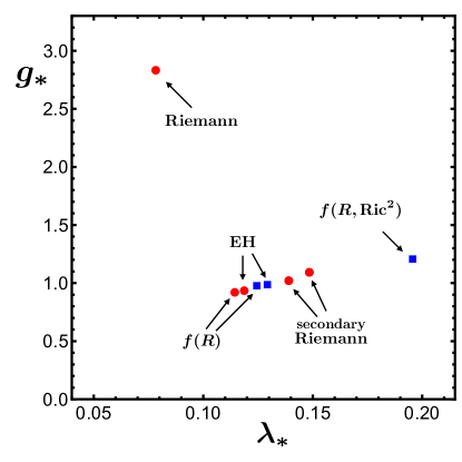
B Cosmological Constant and Newton’s Coupling
Next, we discuss more specifically the impact of higher dimensional curvature interactions on the fixed points for Newton’s coupling and the cosmological constant. To that end, Fig. 25 zooms into Fig. 2 to show the values for the fixed point couplings at the Riemann fixed points, and in comparison to other models and approximations.
The colour coding in Fig. 25 (blue squares vs red dots) distinguishes underlying technical choices. Results indicated by blue squares use the heat kernel expansion alongside optimised cutoff functions Litim:2001up ; Litim:2003vp , and gauge fixing parameters identical to those first adopted by Codello, Percacci and Rahmede Codello:2007bd for polynomial models. The same technical setting has been used for high order models in Falls:2013bv ; Falls:2014tra . Subsequently, new flow equations have been derived for models, again using the same technical choices Falls:2017lst ; see Fig. 1.
Results indicated by red dots use the heat kernel expansion with optimised cutoff functions Litim:2001up ; Litim:2003vp , and the same gauge fixing parameters as in Codello:2007bd , except that ghost fields are now treated differently to ensure that unphysical, convergence-limiting poles of the flow are removed from the outset Falls:2018ylp . The new treatment of ghosts leads to quantitative, and also qualitative differences. Most notably, models with improved ghosts display real de Sitter solutions Falls:2018ylp . Without improved ghosts, de Sitter solutions disappear narrowly into the complex field plane Falls:2016wsa .
A few points are worth emphasizing in Fig. 25. We note that results for fixed point couplings are very close to those for the Einstein-Hilbert (EH) approximation. Higher order interactions lead to a small reduction of while leaving mostly unchanged. This pattern is neatly visible irrespective of the presence or absence of ghost-induced poles. The small quantitative differences are entirely due to the additional type interactions beyond the Einstein-Hilbert terms. Turning now to the models with Ricci and Riemann tensor interactions, we notice that the inclusion of Ricci tensors, leads to a more substantial increase of the cosmological constant , alongside a moderate increase in . The same holds true at the secondary Riemann fixed points, which also show a moderate increase in over the Einstein Hilbert result. On the other hand, the primary Riemann fixed point shows a substantial increase of and a decrease in over findings in the EH and approximations. Incidentally, the strong shift in the value for is also at the root for the slow convergence of the polynomial expansion at the first few orders observed previously (see Tab. 2). We conclude from Fig. 25 that theories with Ricci and Riemann tensor interactions lead to more substantial alterations of the fixed point couplings and over the Einstein-Hilbert and approximations. Hence, the pattern of alterations is quite sensitive to whether the interactions involve Ricci scalars, tensors, or Riemann tensors.
C Interaction Strength and Perturbativity
The gravitational couplings by themselves are not universal quantities at a fixed point. Still, some universal quantities of interest are given by products of couplings which remain invariant under a rescaling of the metric field
| (86) |
In our conventions, the gravitational couplings (33) transform as under the rescaling (86) in four dimensions. Clearly, many scale invariant products can be formed out of the fixed point couplings Falls:2014tra . Kawai and Ninomiya Kawai:1989yh have explained that the scale-invariant product of the lowest-order couplings is of particular interest in that it serves as an indicator for the effective gravitational coupling strength. It will then be useful to compare different fixed point theories from the viewpoint of their effective coupling strength.
In our settings, the effective coupling strength is given by the product in terms of the dimensionless cosmological constant and Newton’s coupling, see (27). In Fig. 26, we show our results for the scale-invariant product at the fixed point, comparing different approximations and using the same colour-coding as in Fig. 25. In the Einstein-Hilbert approximation, we find
| (87) |
Here, the range indicates the small variations due to different treatment of ghosts. Moreover, it is also well-known that this product is rather stable under alterations of the RG scheme, the shape of the Wilsonian momentum cutoff, and under changes of gauge fixing parameters Lauscher:2001ya ; Fischer:2006fz ; Falls:2014zba . The smallness of the result may be taken as an indicator for the weakness of gravitational interactions at an asymptotically safe UV fixed point. Within models for quantum gravity, findings for the effective coupling strength are in the range of
| (88) |
The rather small decrease of the effective coupling strength over (87) is due to the combined small decrease in and . This is in accord with the picture laid out above, in particular Fig. 25. We conclude that the presence of higher order Ricci scalar interactions has only a very mild impact on this universal parameter. This result also confirms the view that the fixed point in type models of quantum gravity can be interpreted as the extension of the fixed point already observed in the much simpler Einstein-Hilbert approximation.
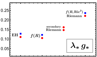
We now turn to models with Ricci tensor or Riemann tensor interactions. Unlike in models with Ricci scalar interactions only, these models also feature fourth order propagating degrees of freedom. In comparison with (87), (88), we observe that the scale-invariant product of couplings is larger by a factor of two for models studied in Falls:2017lst ,
| (89) |
This is due to a strong increase in and a small increase in , as can be seen from Fig. 25. In combination, these alterations make the effective coupling strength twice as large as in models with Ricci scalar interactions. Finally, for models studied in this work, we have
| (90) |
which once more is larger than (87), (88) by a factor of two. Here, the enhancement is due to a substantial increase in in combination with a small decrease in , see Fig. 25. It is quite intriguing that fixed point theories from Ricci tensor or Riemann tensor interactions both lead to very similar values for the scale-invariant interaction strength (Fig. 26). Finally, for the secondary Riemann fixed points we have
| (91) |
see (65) and (67). Quantitatively, this is closer to the EH result (87) than to (90), owing to the fact that the fixed point coordinates only differ mildly from the EH result. Still, for either of these the additional Riemann interactions increase the scale-invariant product of couplings over the Einstein Hilbert values, much unlike in models (88).
The comparison of results in Fig. 26 shows that Ricci and Riemann tensor interactions increase, while Ricci scalar decrease the quantity . This indicates that the additional degrees of freedom in theories with Ricci tensor or Riemann tensor interactions make the theory more strongly coupled, roughly by up to a factor of two, and irrespective of the finer details for the higher dimensional interaction terms. In this light, the closeness of (89) and (90) can be seen as an indication for universality. At the same time, the quantitative smallness of (89) and (90), albeit twice as large as (87), (88), and the near-Gaussianity of scaling exponents with increasing mass dimension (see Sec. E) still indicates that the fixed point theory is largely weakly coupled. All in all, this further substantiates the view that quantum gravity remains ”as Gaussian as it gets” to accommodate non-perturbative renormalisability Falls:2013bv ; Falls:2014tra ; Falls:2017lst ; Falls:2018ylp .
D Quantum Vacuum
Finally, we compare solutions to the quantum equations of motion , the ‘vacuum’ solutions, which in our models correspond to field configurations of constant Ricci scalar curvature. In our study, vacuum solutions have been found both at the primary Riemann fixed point (41), (44), and at the secondary ones (74), in accord with expectations Dietz:2013sba .
We compare the vacuum solutions with those from the Einstein Hilbert approximation (42), and the Falls:2018ylp and fixed point Falls:2017lst , shown in Fig. 27, with denoting the background Ricci scalar curvature in units of the RG scale. We use once more the same colour-coding as in Fig. 25. Taking the Einstein Hilbert approximation with the Reuter fixed point as a point of reference, we see that the treatment of ghost only makes a minor difference, with roughly for either of the settings.
For the Riemann fixed points, we see that the secondary ones have nearby vacuum solutions with . This is in accord with the view that these fixed points can be considered as natural extensions of the Reuter fixed point. The vacuum solution for the primary Riemann fixed point is much smaller, around . This effect is entirely due to the coupling being much larger and much smaller than their EH counterparts. Moreover, all three Riemann fixed points share the feature that their vacuum solutions are controlled by the cosmological constant , and by Newton’s coupling and the Ricci scalar term in the action. Consequently, all higher order Riemann interaction terms only add a small subleading contribution to . Turning to and models, we note that both have vacuum solutions in the range of , roughly twice as large as those at the Reuter fixed point. Here, the enhancement is entirely due to higher order interaction terms in the effective action, rather than to a softening of or an enhancement of . Also, for models the improved treatment of ghosts (red dot) makes an important difference Falls:2018ylp . Without it, the vacuum solution has a small complex component Falls:2016wsa as indicated by brackets around the corresponding data point (blue square) in Fig. 27.
We conclude that higher order Ricci scalar, Ricci tensor or Riemann tensor interactions affect the location of vacuum solutions in vastly different manners. One may speculate that those vacuum solutions related to models with a larger UV critical surface are more likely to be realised in the full (un-approximated) theory of asymptotically safe quantum gravity. However, this remains to be clarified in future works.
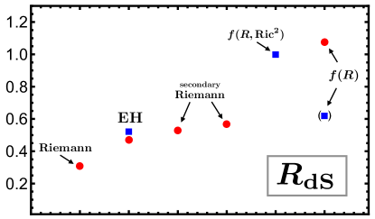
VIII Summary and Conclusions
Starting from gravitational actions involving Ricci scalars, tensors, and Riemann tensors, we have derived a new family of functional renormalisation group equations for the running gravitational couplings. This completes a line of work initiated in Falls:2014tra ; Falls:2017lst ; Falls:2018ylp , and allows systematic studies of quantum gravity including a large variety of higher order curvature invariants. Different parameter choices correspond to different rays in the space of gravitational actions after projection onto the sphere, much in the spirit of a local potential approximation Benedetti:2012dx . The setting is versatile and, together with the known heat kernel coefficients Kluth:2019vkg , can be used to explore quantum effects for higher curvature extensions of general relativity Sotiriou:2008rp ; DeFelice:2010aj ; Clifton:2011jh ; Capozziello:2011et or holography Hung:2011xb , the role of higher order curvature interactions for the asymptotic safety conjecture as done here, and the inclusion of matter, or more general gauge fixing conditions and cutoff profiles.
We have applied the formalism to models of quantum gravity with Riemann interactions. Using polynomial expansions of the action to high order a primary Riemann fixed point has been found satisfying all standard tests including a fast convergence of couplings (Fig. 4) and scaling exponents (Fig. 9), the bootstrap test (Fig. 12), near-Gaussian behaviour at large orders (Fig. 13), and a maximal radius of convergence (Fig. 5 and Fig. 6). High order polynomial expansions of the action up to 144 powers in curvature have been used to establish convergence and stability. Together with numerical integration, they have also been used to obtain solutions beyond any polynomial order. Findings differ noticeably from those in Einstein-Hilbert and approximations (Fig. 25) and come out more strongly coupled (Fig. 26). We have also found a stable pair of weakly coupled Riemann fixed points including de Sitter solutions and well-defined UV-IR connecting RG trajectories with General Relativity at low energies. For these, the leading couplings and scaling exponents are close to those of the Einstein-Hilbert fixed point (Fig. 2) with elsewise mild quantum corrections. For these reasons, they can be viewed as higher curvature extensions of the Reuter fixed point.
An important novelty is the dimensionality of the critical surface which is found to be four (Figs. 11 and 17). This is rather different from models without Riemann tensor interactions, where the critical surface – with all other technical choices the same – comes out as three-dimensional. Our study highlights that quantum-induced shifts in the scaling dimensions of the order of a few (Fig. 15) may well turn canonically irrelevant dim-6 operators into relevant ones. The smallness of the scale-invariant product of couplings and the near-Gaussianity of high order scaling dimensions further substantiates the view that quantum gravity remains ”as Gaussian as it gets”. Future work should investigate the relevancy of other dim-6 curvature invariants (Tab. 1), and other technical choices, to further substantiate the number of fundamentally free parameters of quantum gravity.
Another novelty of this work is the detailed study of eigenvectors and eigenperturbations in the ultraviolet.
Eigenvectors are nonuniversal quantities which change under rescalings of couplings
(Fig. 22). We have shown that a simple equal weight condition
leads to order-by-order stable eigenvectors
which represent the relevant physics correctly (Figs. 23, 24).
Results further substantiate that relevant eigenperturbations are linear combinations of the leading handful of interaction terms, with irrelevant ones dominated by subleading interactions. Anomalous dimensions are found to be of order unity,
having the largest impact on interaction monomials with low mass dimension. Eigenvectors are seen to align accordingly.
It will be interesting to exploit these ideas for other theories at criticality, with or without gravity.
Acknowledgments
YK is supported by the Science Technology and Facilities Council (STFC) under grant number [ST/S505766/1]. Some of our results have been presented at the workshops Asymptotic Safety Meets Particle Physics V (U Dortmund, Dec 2018), Beyond the Standard Model XXXI (Bad Honnef, Mar 2019), and at the workshop Quantum and Gravity (U Okinawa, Jul 2019). YK thanks the organisers for hospitality and participants for discussions.
Appendices
In the appendix, we summarise some of the technical expressions and formulæ required in the main text, including first and second variations of the basic field monomials in the action (App. A), the Hessians of the effective action (App. B), and the general form of the functional flow equations (App. C).
A First and Second Variations
In the main text, we require the first two variations of
| (A.1) |
subject to the linear split (10) in general dimension. The first variation is given by
| (A.2) |
while the second variation gives
| (A.3) |
B Hessians
C Flow Equation and Fluctuation Integrals
The central flow equation (14) of this work arises from (1) with (2), (13). Adopting the cutoff (16) and evaluating all operator traces, the explicit flow takes the form
| (C.1) |
with . Here, we specify the fluctuation-induced terms contained in the fluctuation integrals on the RHS. Adopting conventions and notation of Falls:2014tra ; Falls:2017lst , we find
| (C.2) |
where we recall that the flow terms arise due to couplings introduced via the regularisation. All five terms arise from tracing over the fluctuations of the metric field for which we have adopted a transverse traceless decomposition. They do not contain any renormalisation scale derivative. The term also receives - and -independent contributions from the ghosts and from the Jacobians originating from the split of the metric fluctuations into tensor, vector and scalar parts. To indicate the origin of the various contributions in the expressions below, we use superscipts , , and to refer to the transverse traceless tensorial, vectorial, and scalar origin. The specific form of the functions also depends on the choice of gauge fixing and the details for the regulator function. In our setting, they are given by
| (C.3) | ||||
The denominators and in (C.3) arise from the tensorial (T) and scalar (S) metric fluctuations, and are defined as
| (C.4) | |||||
The various terms in (C.3) are polynomials in curvature. Specifically, the terms and are given by
| (C.6) | |||||
| (C.7) |
The numerators appearing in (C.3) can be written as
| (C.8) | |||||
| (C.9) |
with coefficient functions
| (C.10) | |||||
| (C.11) | |||||
| (C.12) | |||||
| (C.13) | |||||
| (C.14) | |||||
| (C.15) | |||||
| (C.16) | |||||
| (C.17) | |||||
| (C.18) | |||||
| (C.19) |
The numerators appearing in (C.3) take the form
| (C.20) |
| (C.21) |
| (C.22) |
| (C.23) |
References
- (1) S. Weinberg, Ultraviolet divergences in quantum theories of gravitation, in: General Relativity: An Einstein centenary survey, Eds. Hawking, S.W., Israel, W; Cambridge University Press (1980) 790.
- (2) K. G. Wilson, Renormalization group and critical phenomena. 1. Renormalization group and the Kadanoff scaling picture, Phys.Rev. B4 (1971) 3174.
- (3) K. G. Wilson, Renormalization group and critical phenomena. 2. Phase space cell analysis of critical behavior, Phys.Rev. B4 (1971) 3184.
- (4) D. F. Litim, On fixed points of quantum gravity, AIP Conf.Proc. 841 (2006) 322 [hep-th/0606044].
- (5) M. Niedermaier, The asymptotic safety scenario in quantum gravity: An introduction, Class. Quant. Grav. 24 (2007) R171 [gr-qc/0610018].
- (6) D. F. Litim, Renormalisation Group and the Planck Scale, Phil. Trans. Roy. Soc. Lond. A 369 (2011) 2759 [1102.4624].
- (7) M. H. Goroff and A. Sagnotti, Quantum Gravity at Two Loops, Phys.Lett. B160 (1985) 81.
- (8) M. H. Goroff and A. Sagnotti, The Ultraviolet Behavior of Einstein Gravity, Nucl.Phys. B266 (1986) 709.
- (9) J. Gomis and S. Weinberg, Are nonrenormalizable gauge theories renormalizable?, Nucl. Phys. B 469 (1996) 473 [hep-th/9510087].
- (10) K. Stelle, Renormalization of Higher Derivative Quantum Gravity, Phys. Rev. D 16 (1977) 953.
- (11) D. Anselmi and M. Piva, The Ultraviolet Behavior of Quantum Gravity, JHEP 05 (2018) 027 [1803.07777].
- (12) D. F. Litim and F. Sannino, Asymptotic safety guaranteed, JHEP 12 (2014) 178 [1406.2337].
- (13) A. D. Bond and D. F. Litim, Theorems for Asymptotic Safety of Gauge Theories, Eur. Phys. J. C77 (2017) 429 [1608.00519].
- (14) T. Buyukbese and D. F. Litim, Asymptotic safety of gauge theories beyond marginal interactions, PoS LATTICE2016 (2017) 233.
- (15) A. D. Bond and D. F. Litim, Asymptotic safety guaranteed in supersymmetry, Phys. Rev. Lett. 119 (2017) 211601 [1709.06953].
- (16) A. D. Bond, D. F. Litim, G. Medina Vazquez and T. Steudtner, UV conformal window for asymptotic safety, Phys. Rev. D97 (2018) 036019 [1710.07615].
- (17) A. D. Bond, D. F. Litim and T. Steudtner, Asymptotic safety with Majorana fermions and new large equivalences, Phys. Rev. D101 (2020) 045006 [1911.11168].
- (18) A. D. Bond and D. F. Litim, Asymptotic safety guaranteed for strongly coupled gauge theories, Phys. Rev. D 105 (2022) 105005 [2202.08223].
- (19) B. Rosenstein, B. J. Warr and S. H. Park, The Four Fermi Theory Is Renormalizable in (2+1)-Dimensions, Phys. Rev. Lett. 62 (1989) 1433.
- (20) C. de Calan, P. Faria da Veiga, J. Magnen and R. Seneor, Constructing the three-dimensional Gross-Neveu model with a large number of flavor components, Phys.Rev.Lett. 66 (1991) 3233.
- (21) A. Jakovac, A. Patkos and P. Posfay, Non-Gaussian fixed points in fermionic field theories without auxiliary Bose-fields, Eur. Phys. J. C75 (2015) [1406.3195].
- (22) C. Cresswell-Hogg and D. F. Litim, Line of Fixed Points in Gross-Neveu Theories, 2207.10115.
- (23) K. Falls, D. Litim, K. Nikolakopoulos and C. Rahmede, A Bootstrap Towards Asymptotic Safety, 1301.4191.
- (24) J. Polchinski, Renormalization and Effective Lagrangians, Nucl.Phys. B231 (1984) 269.
- (25) C. Wetterich, Exact evolution equation for the effective potential, Phys.Lett. B301 (1993) 90.
- (26) T. R. Morris, The Exact renormalization group and approximate solutions, Int. J. Mod. Phys. A 9 (1994) 2411 [hep-ph/9308265].
- (27) M. Reuter, Nonperturbative Evolution Equation for Quantum Gravity, Phys. Rev. D57 (1998) 971 [hep-th/9605030].
- (28) F. Freire, D. F. Litim and J. M. Pawlowski, Gauge invariance and background field formalism in the exact renormalization group, Phys. Lett. B 495 (2000) 256 [hep-th/0009110].
- (29) D. F. Litim, Optimized renormalization group flows, Phys. Rev. D64 (2001) 105007 [hep-th/0103195].
- (30) W. Souma, Nontrivial ultraviolet fixed point in quantum gravity, Prog. Theor. Phys. 102 (1999) 181 [hep-th/9907027].
- (31) W. Souma, Gauge and cutoff function dependence of the ultraviolet fixed point in quantum gravity, gr-qc/0006008.
- (32) M. Reuter and F. Saueressig, Renormalization group flow of quantum gravity in the Einstein-Hilbert truncation, Phys. Rev. D65 (2002) 065016 [hep-th/0110054].
- (33) O. Lauscher and M. Reuter, Ultraviolet fixed point and generalized flow equation of quantum gravity, Phys. Rev. D65 (2002) 025013 [hep-th/0108040].
- (34) D. F. Litim, Fixed points of quantum gravity, Phys. Rev. Lett. 92 (2004) 201301 [hep-th/0312114].
- (35) A. Bonanno and M. Reuter, Proper time flow equation for gravity, JHEP 02 (2005) 035 [hep-th/0410191].
- (36) P. Fischer and D. F. Litim, Fixed points of quantum gravity in extra dimensions, Phys.Lett. B638 (2006) 497 [hep-th/0602203].
- (37) D. F. Litim, Fixed Points of Quantum Gravity and the Renormalisation Group, PoS QG-Ph (2007) 024 [0810.3675].
- (38) A. Eichhorn, H. Gies and M. M. Scherer, Asymptotically free scalar curvature-ghost coupling in Quantum Einstein Gravity, Phys. Rev. D80 (2009) 104003 [0907.1828].
- (39) E. Manrique and M. Reuter, Bimetric Truncations for Quantum Einstein Gravity and Asymptotic Safety, Annals Phys. 325 (2010) 785 [0907.2617].
- (40) A. Eichhorn and H. Gies, Ghost anomalous dimension in asymptotically safe quantum gravity, Phys. Rev. D81 (2010) 104010 [1001.5033].
- (41) E. Manrique, M. Reuter and F. Saueressig, Bimetric Renormalization Group Flows in Quantum Einstein Gravity, Annals Phys. 326 (2011) 463 [1006.0099].
- (42) E. Manrique, S. Rechenberger and F. Saueressig, Asymptotically Safe Lorentzian Gravity, Phys.Rev.Lett. 106 (2011) 251302 [1102.5012].
- (43) D. Litim and A. Satz, Limit cycles and quantum gravity, 1205.4218.
- (44) I. Donkin and J. M. Pawlowski, The phase diagram of quantum gravity from diffeomorphism-invariant RG-flows, 1203.4207.
- (45) N. Christiansen, D. F. Litim, J. M. Pawlowski and A. Rodigast, Fixed points and infrared completion of quantum gravity, Phys.Lett. B728 (2014) 114 [1209.4038].
- (46) A. Codello, G. D’Odorico and C. Pagani, Consistent closure of renormalization group flow equations in quantum gravity, Phys. Rev. D89 (2014) 081701 [1304.4777].
- (47) N. Christiansen, B. Knorr, J. M. Pawlowski and A. Rodigast, Global Flows in Quantum Gravity, Phys. Rev. D93 (2016) 044036 [1403.1232].
- (48) D. Becker and M. Reuter, En route to Background Independence: Broken split-symmetry, and how to restore it with bi-metric average actions, Annals Phys. 350 (2014) 225 [1404.4537].
- (49) K. Falls, Asymptotic safety and the cosmological constant, JHEP 01 (2016) 069 [1408.0276].
- (50) K. Falls, Renormalization of Newton’s constant, Phys. Rev. D92 (2015) 124057 [1501.05331].
- (51) K. Falls, Critical Scaling in Quantum Gravity from the Renormalisation Group, 1503.06233.
- (52) N. Christiansen, B. Knorr, J. Meibohm, J. M. Pawlowski and M. Reichert, Local Quantum Gravity, Phys. Rev. D92 (2015) 121501 [1506.07016].
- (53) H. Gies, B. Knorr and S. Lippoldt, Generalized Parametrization Dependence in Quantum Gravity, Phys. Rev. D92 (2015) 084020 [1507.08859].
- (54) D. Benedetti, Essential nature of Newton’s constant in unimodular gravity, Gen. Rel. Grav. 48 (2016) 68 [1511.06560].
- (55) J. Biemans, A. Platania and F. Saueressig, Quantum gravity on foliated spacetimes: Asymptotically safe and sound, Phys. Rev. D95 (2017) 086013 [1609.04813].
- (56) C. Pagani and M. Reuter, Composite Operators in Asymptotic Safety, Phys. Rev. D95 (2017) 066002 [1611.06522].
- (57) K. Falls, Physical renormalization schemes and asymptotic safety in quantum gravity, Phys. Rev. D 96 (2017) 126016 [1702.03577].
- (58) W. B. Houthoff, A. Kurov and F. Saueressig, Impact of topology in foliated Quantum Einstein Gravity, Eur. Phys. J. C77 (2017) 491 [1705.01848].
- (59) B. Knorr and S. Lippoldt, Correlation functions on a curved background, Phys. Rev. D96 (2017) 065020 [1707.01397].
- (60) O. Lauscher and M. Reuter, Flow equation of quantum Einstein gravity in a higher- derivative truncation, Phys. Rev. D66 (2002) 025026 [hep-th/0205062].
- (61) A. Codello and R. Percacci, Fixed Points of Higher Derivative Gravity, Phys. Rev. Lett. 97 (2006) 221301 [hep-th/0607128].
- (62) A. Codello, R. Percacci and C. Rahmede, Ultraviolet properties of f(R)-gravity, Int. J. Mod. Phys. A23 (2008) 143 [0705.1769].
- (63) P. F. Machado and F. Saueressig, On the renormalization group flow of f(R)-gravity, Phys. Rev. D77 (2008) 124045 [0712.0445].
- (64) A. Codello, R. Percacci and C. Rahmede, Investigating the Ultraviolet Properties of Gravity with a Wilsonian Renormalization Group Equation, Annals Phys. 324 (2009) 414 [0805.2909].
- (65) D. Benedetti, P. F. Machado and F. Saueressig, Asymptotic safety in higher-derivative gravity, Mod. Phys. Lett. A24 (2009) 2233 [0901.2984].
- (66) D. Benedetti, P. F. Machado and F. Saueressig, Taming perturbative divergences in asymptotically safe gravity, Nucl. Phys. B824 (2010) 168 [0902.4630].
- (67) D. Benedetti, K. Groh, P. F. Machado and F. Saueressig, The Universal RG Machine, JHEP 1106 (2011) 079 [1012.3081].
- (68) M. Niedermaier, Can a nontrivial gravitational fixed point be identified in perturbation theory?, PoS CLAQG08 (2011) 005.
- (69) M. R. Niedermaier, Gravitational Fixed Points from Perturbation Theory, Phys. Rev. Lett. 103 (2009) 101303.
- (70) M. Niedermaier, Gravitational fixed points and asymptotic safety from perturbation theory, Nucl.Phys. B833 (2010) 226.
- (71) K. Groh, S. Rechenberger, F. Saueressig and O. Zanusso, Higher Derivative Gravity from the Universal Renormalization Group Machine, PoS EPS-HEP2011 (2011) 124 [1111.1743].
- (72) D. Benedetti and F. Caravelli, The Local potential approximation in quantum gravity, JHEP 06 (2012) 017 [1204.3541].
- (73) J. A. Dietz and T. R. Morris, Asymptotic safety in the f(R) approximation, JHEP 01 (2013) 108 [1211.0955].
- (74) N. Ohta and R. Percacci, Higher Derivative Gravity and Asymptotic Safety in Diverse Dimensions, Class. Quant. Grav. 31 (2014) 015024 [1308.3398].
- (75) D. Benedetti, On the number of relevant operators in asymptotically safe gravity, Europhys. Lett. 102 (2013) 20007 [1301.4422].
- (76) J. A. Dietz and T. R. Morris, Redundant operators in the exact renormalisation group and in the f(R) approximation to asymptotic safety, JHEP 07 (2013) 064 [1306.1223].
- (77) K. Falls, D. F. Litim, K. Nikolakopoulos and C. Rahmede, Further evidence for asymptotic safety of quantum gravity, Phys. Rev. D93 (2016) 104022 [1410.4815].
- (78) I. D. Saltas, UV structure of quantum unimodular gravity, Phys. Rev. D90 (2014) 124052 [1410.6163].
- (79) M. Demmel, F. Saueressig and O. Zanusso, RG flows of Quantum Einstein Gravity on maximally symmetric spaces, 1401.5495.
- (80) A. Eichhorn, The Renormalization Group flow of unimodular f(R) gravity, JHEP 04 (2015) 096 [1501.05848].
- (81) N. Ohta, R. Percacci and G. P. Vacca, Flow equation for gravity and some of its exact solutions, Phys. Rev. D92 (2015) 061501 [1507.00968].
- (82) N. Ohta, R. Percacci and G. P. Vacca, Renormalization Group Equation and scaling solutions for f(R) gravity in exponential parametrization, Eur. Phys. J. C76 (2016) 46 [1511.09393].
- (83) M. Demmel, F. Saueressig and O. Zanusso, A proper fixed functional for four-dimensional Quantum Einstein Gravity, JHEP 08 (2015) 113 [1504.07656].
- (84) K. Falls, D. F. Litim, K. Nikolakopoulos and C. Rahmede, On de Sitter solutions in asymptotically safe theories, Class. Quant. Grav. 35 (2018) 135006 [1607.04962].
- (85) K. Falls and N. Ohta, Renormalization Group Equation for gravity on hyperbolic spaces, Phys. Rev. D94 (2016) 084005 [1607.08460].
- (86) H. Gies, B. Knorr, S. Lippoldt and F. Saueressig, Gravitational Two-Loop Counterterm Is Asymptotically Safe, Phys. Rev. Lett. 116 (2016) 211302 [1601.01800].
- (87) N. Christiansen, Four-Derivative Quantum Gravity Beyond Perturbation Theory, 1612.06223.
- (88) S. Gonzalez-Martin, T. R. Morris and Z. H. Slade, Asymptotic solutions in asymptotic safety, Phys. Rev. D95 (2017) 106010 [1704.08873].
- (89) D. Becker, C. Ripken and F. Saueressig, On avoiding Ostrogradski instabilities within Asymptotic Safety, JHEP 12 (2017) 121 [1709.09098].
- (90) K. Falls, C. R. King, D. F. Litim, K. Nikolakopoulos and C. Rahmede, Asymptotic safety of quantum gravity beyond Ricci scalars, Phys. Rev. D97 (2018) 086006 [1801.00162].
- (91) K. G. Falls, D. F. Litim and J. Schröder, Aspects of Asymptotic Safety for Quantum Gravity, Phys. Rev. D 99 (2019) 126015 [1810.08550].
- (92) G. P. De Brito, N. Ohta, A. D. Pereira, A. A. Tomaz and M. Yamada, Asymptotic safety and field parametrization dependence in the truncation, Phys. Rev. D98 (2018) 026027 [1805.09656].
- (93) K. Falls, N. Ohta and R. Percacci, Towards the Determination of the Dimension of the Critical Surface in Asymptotically Safe Gravity, 2004.04126.
- (94) T. P. Sotiriou and V. Faraoni, f(R) Theories Of Gravity, Rev. Mod. Phys. 82 (2010) 451 [0805.1726].
- (95) A. De Felice and S. Tsujikawa, f(R) theories, Living Rev. Rel. 13 (2010) 3 [1002.4928].
- (96) T. Clifton, P. G. Ferreira, A. Padilla and C. Skordis, Modified Gravity and Cosmology, Phys. Rept. 513 (2012) 1 [1106.2476].
- (97) S. Capozziello and M. De Laurentis, Extended Theories of Gravity, Phys. Rept. 509 (2011) 167 [1108.6266].
- (98) L.-Y. Hung, R. C. Myers and M. Smolkin, On Holographic Entanglement Entropy and Higher Curvature Gravity, JHEP 04 (2011) 025 [1101.5813].
- (99) Y. Kluth and D. F. Litim, Functional renormalization for f(R) quantum gravity, Phys. Rev. D 106 (2022) 106022 [2202.10436].
- (100) R. Percacci, An Introduction to Covariant Quantum Gravity and Asymptotic Safety, vol. 3 of 100 Years of General Relativity. World Scientific, 2017, 10.1142/10369.
- (101) M. Reuter and F. Saueressig, Quantum Gravity and the Functional Renormalization Group: The Road Towards Asymptotic Safety. Cambridge University Press, 1, 2019.
- (102) H. Kawai, Y. Kitazawa and M. Ninomiya, Scaling exponents in quantum gravity near two-dimensions, Nucl. Phys. B393 (1993) 280 [hep-th/9206081].
- (103) H. Kawai, Y. Kitazawa and M. Ninomiya, Ultraviolet stable fixed point and scaling relations in (2+epsilon)-dimensional quantum gravity, Nucl.Phys. B404 (1993) 684 [hep-th/9303123].
- (104) A. Nink, Field Parametrization Dependence in Asymptotically Safe Quantum Gravity, Phys. Rev. D91 (2015) 044030 [1410.7816].
- (105) D. F. Litim, Optimization of the exact renormalization group, Phys. Lett. B486 (2000) 92 [hep-th/0005245].
- (106) I. G. Avramidi, Heat kernel and quantum gravity, Lect. Notes Phys. Monogr. 64 (2000) 1.
- (107) Y. Kluth and D. F. Litim, Heat Kernel Coefficients on the Sphere in Any Dimension, Eur. Phys. J. C 80 (2020) 269 [1910.00543].
- (108) J. Nicoll, T. Chang and H. Stanley, Nonlinear Solutions of Renormalization-Group Equations, Phys. Rev. Lett. 32 (1974) 1446.
- (109) D. Baumann, Inflation, in Physics of the large and the small, TASI 09, proceedings of the Theoretical Advanced Study Institute in Elementary Particle Physics, Boulder, Colorado, USA, 1-26 June 2009, pp. 523–686, 2011, 0907.5424, DOI.
- (110) M. Hindmarsh, D. Litim and C. Rahmede, Asymptotically Safe Cosmology, JCAP 1107 (2011) 019 [1101.5401].
- (111) A. Baldazzi, R. Percacci and V. Skrinjar, Wicked metrics, Class. Quant. Grav. 36 (2019) 105008 [1811.03369].
- (112) A. Bonanno, T. Denz, J. M. Pawlowski and M. Reichert, Reconstructing the graviton, SciPost Phys. 12 (2022) 001 [2102.02217].
- (113) J. Fehre, D. F. Litim, J. M. Pawlowski and M. Reichert, Lorentzian Quantum Gravity and the Graviton Spectral Function, Phys. Rev. Lett. 130 (2023) 081501 [2111.13232].
- (114) A. Bonanno, A. Contillo and R. Percacci, Inflationary solutions in asymptotically safe f(R) theories, Class. Quant. Grav. 28 (2011) 145026 [1006.0192].
- (115) D. F. Litim and D. Zappala, Ising exponents from the functional renormalisation group, Phys. Rev. D 83 (2011) 085009 [1009.1948].
- (116) D. F. Litim, Mind the gap, Int. J. Mod. Phys. A16 (2001) 2081 [hep-th/0104221].
- (117) T. R. Morris, On truncations of the exact renormalization group, Phys. Lett. B 334 (1994) 355 [hep-th/9405190].
- (118) K.-I. Aoki, K. Morikawa, W. Souma, J.-I. Sumi and H. Terao, Rapidly converging truncation scheme of the exact renormalization group, Prog. Theor. Phys. 99 (1998) 451 [hep-th/9803056].
- (119) D. F. Litim, Derivative expansion and renormalization group flows, JHEP 11 (2001) 059 [hep-th/0111159].
- (120) D. F. Litim, Critical exponents from optimized renormalization group flows, Nucl. Phys. B 631 (2002) 128 [hep-th/0203006].
- (121) D. F. Litim and E. Marchais, Critical models in the complex field plane, Phys. Rev. D95 (2017) 025026 [1607.02030].
- (122) C. Bervillier, B. Boisseau and H. Giacomini, Analytical approximation schemes for solving exact renormalization group equations in the local potential approximation, Nucl. Phys. B 789 (2008) 525 [0706.0990].
- (123) D. F. Litim, E. Marchais and P. Mati, Fixed points and the spontaneous breaking of scale invariance, Phys. Rev. D95 (2017) 125006 [1702.05749].
- (124) A. Jüttner, D. F. Litim and E. Marchais, Global Wilson–Fisher fixed points, Nucl. Phys. B921 (2017) 769 [1701.05168].
- (125) H. Kawai and M. Ninomiya, Renormalization Group and Quantum Gravity, Nucl. Phys. B 336 (1990) 115.