Supplementary Material – Weakly-supervised 3D Shape Completion in the Wild

1 Overview

This supplementary material provides more detailed and thorough analysis of our weakly-supervised approach for 3D shape completion. We hope readers can gain more insights into our approach. Sec 2 presents ablation studies to analyze our design. We report the results of partial point cloud registration on ShapeNet in Sec 3, to show more quantitative comparison. Moreover, we showcase an experiment where the model is fine-tuned on another category in the wild during inference in Sec 4. Sec 6 shows more visual comparison on both synthetic and real LiDAR datasets. Last but not least, the sensitivity to initialization is investigated in Sec 7.

2 Ablation studies

For ablation studies, we investigate several factors: 1) the shape-projection-matching-observation term, 2) the hindsight loss. Table 1 shows the quantitative results on ShapeNet. It is observed that: 1) Without the shape-projection-matching-observation term, the chamfer distance and precision increase while the coverage decreases. It shows the effectiveness of our proposed projection approach, and verifies that the observation-matching-shape term only is not enough as it can not force the generated shape to be close to the observation. On our 3D vehicle dataset, the shape-projection-matching-observation term decreases the precision but increases the coverage, which results in the chamfer distance similar to that without it. However, the loss term can improve visual results. 2) Without the hindsight loss, the network is vulnerable to local minima, and performs worse.

Category	Method	CD	Precision	Coverage
Airplane	w/o projection	2.80	1.98	0.82
	w/o hindsight	2.32	1.18	1.14
	full	1.65	0.77	0.88
Car	w/o projection	2.96	1.67	1.29
	w/o hindsight	2.82	1.46	1.36
	full	2.68	1.27	1.41
Chair	w/o projection	3.94	2.50	1.44
	w/o hindsight	3.80	2.09	1.71
	full	3.33	1.69	1.64

Table 1: Ablation studies on ShapeNet. We report shape completion results on the test set. All the values are multiplied by 100.

In addition, we investigate the relation between the performance and the number of views during training. Table 2 shows results on our 3D vehicle dataset, w.r.t numbers of views. With the same number of instances in a batch, the more the number of views, the better the performance is. We select 4 views per instance as a trade-off between the performance and the computation.

#views	#inst	CD	Rot $\Delta\theta$	Trans $\Delta t$
2	8	0.307	6.185	0.213
4	8	0.261	4.208	0.160
8	8	0.242	3.995	0.142

Table 2: Ablation studies on our 3D vehicle dataset w.r.t different numbers of views. Note that we report an average of 5 trials instead of the best trial here.

3 Point cloud registration on ShapeNet

Input(Ours)

GT

DPC

Ours

Ours*

Figure 1: Qualitative results of 3D shape completion on the test set of ShapeNet. All the point clouds are transformed to the ground-truth canonical frame and visualized at a fixed viewpoint.

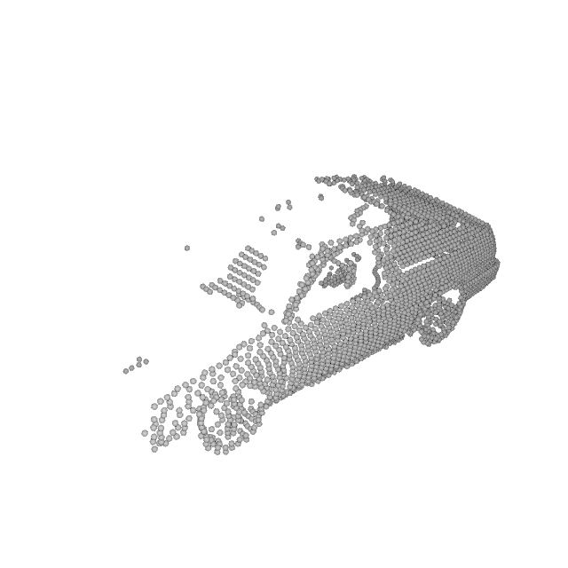
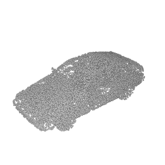
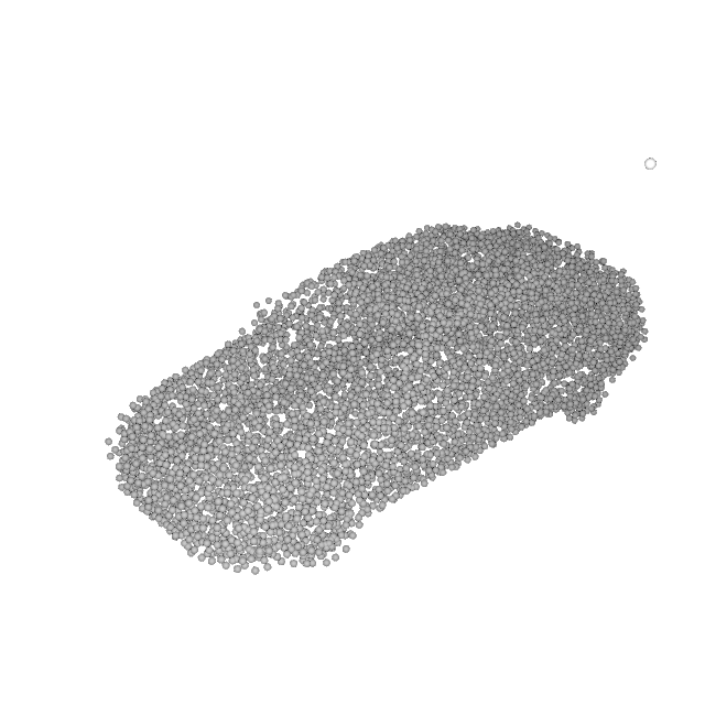
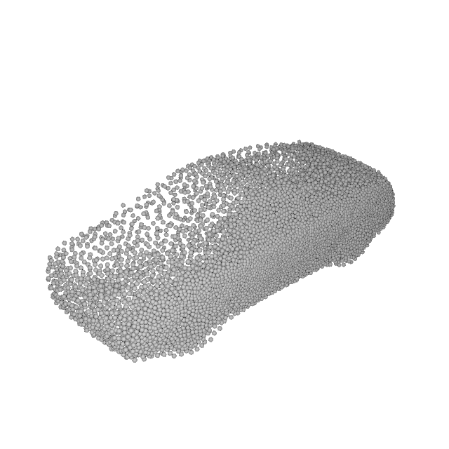
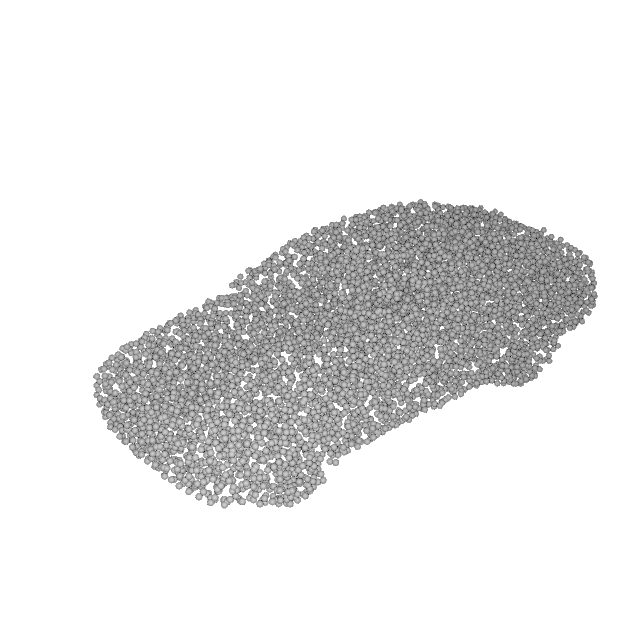
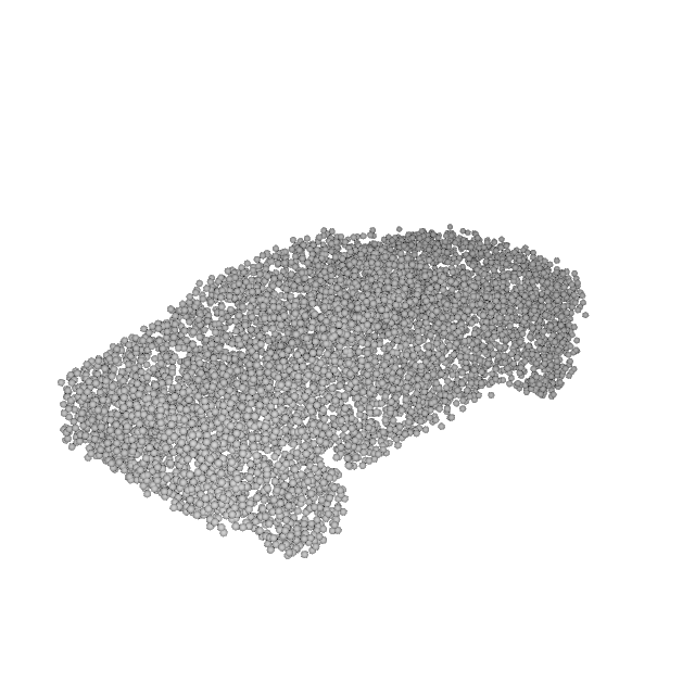
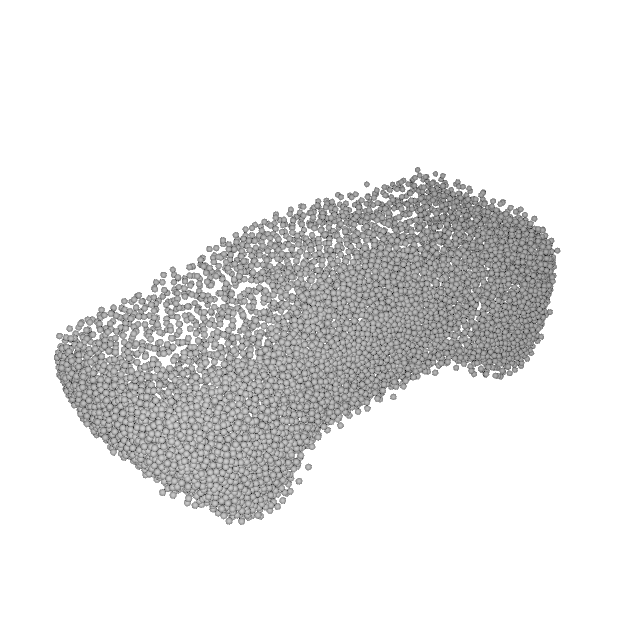
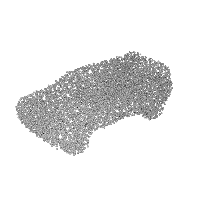
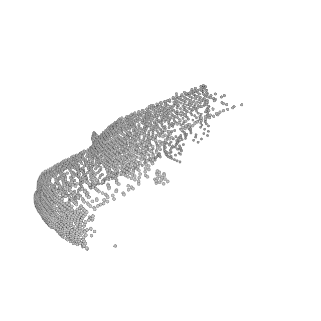
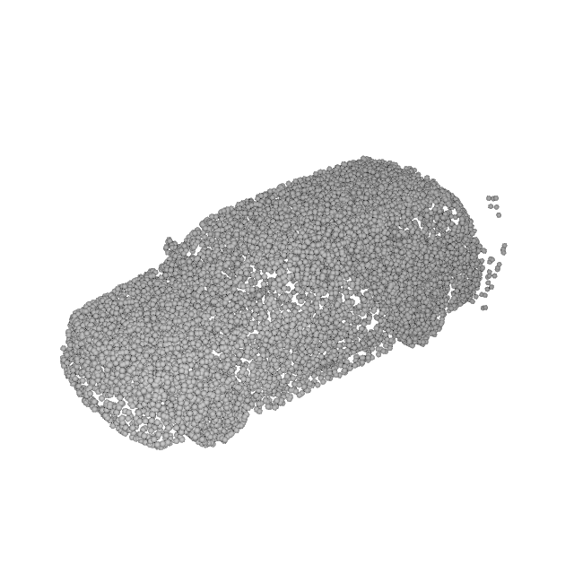
In the main paper, we have showcased that our approach can be extended to challenging partial point cloud registration on real datasets. In this section, we demonstrate the results of this task on ShapeNet. Concretely, we compare the relative pose between one view and the target view against the ground truth relative pose. We argue that our evaluation protocal for pose estimation is better than that in DPC [1], as they measure the pose error by first aligning the canonical pose learned with the groundtruth using ICP. Compared to real datasets with over 80 scans per instance, it is even challenging for synthetic data, since there are only 5 views per object in total for training.

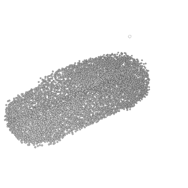
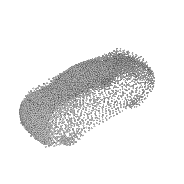
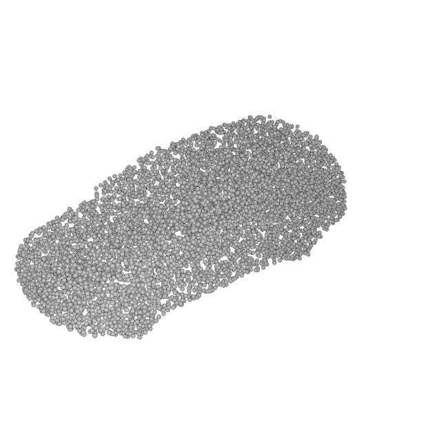
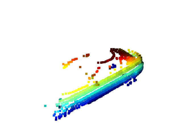
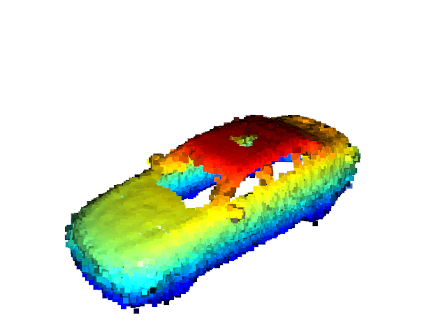
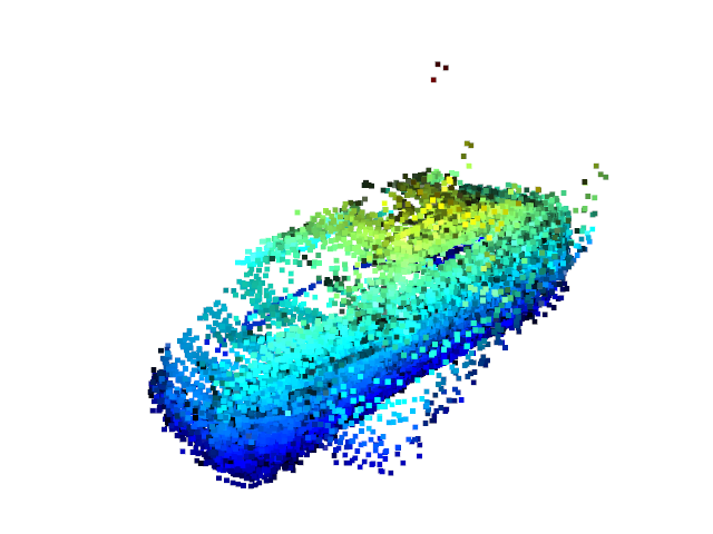
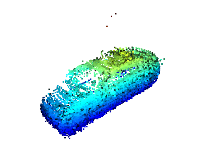
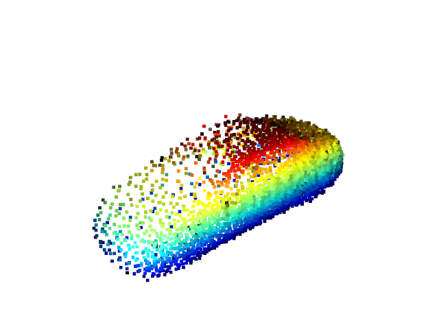
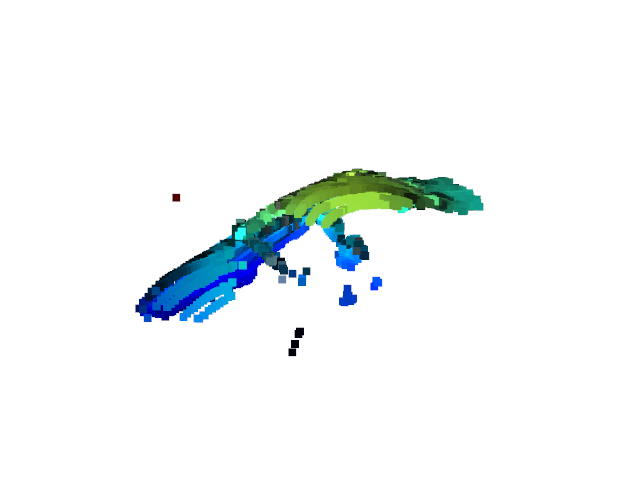
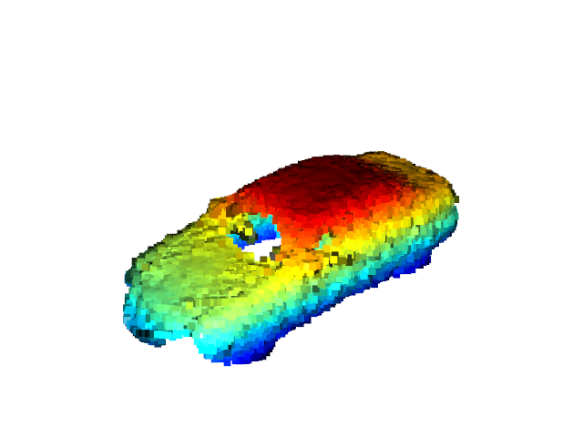
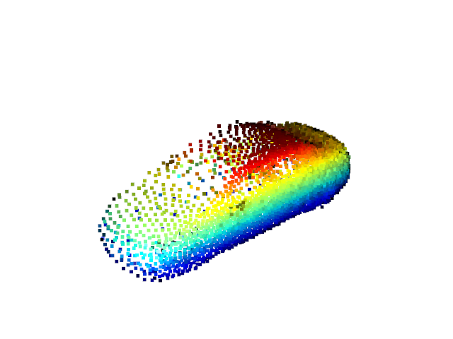
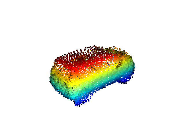
We report the accuracy, median angle difference, and median translation MSE of our method, DPC, DPC^† in Table 3. Our approach outperforms DPC and DPC^† by a large margin on all the categories. For cars, we use a variant of our approach, where input and output points are both projected into 2D points and the chamfer distance between 2D projections is optimized. Unlike chairs and planes, the front and back of cars look similar, which introduces more pose ambiguity and results in an oversmoothed canonical shape. Thus, the variant is proposed to tackle the pose ambiguity caused by the symmetry of cars. Fig 1 shows the comparison between the variant (Ours^∗) and the original implementation.

Category	Method	Acc($\Delta\theta\leq 30^{\circ}$)	Rot $\Delta\theta$	Trans $\Delta t$
Airplane	DPC	74.17	9.95	-
	DPC†	55.64	23.85	0.13
	Ours	92.87	1.87	0.01
Car	DPC	84.75	6.40	-
	DPC†	82.17	8.79	0.05
	Ours*	91.03	2.46	-
Chair	DPC	80.02	10.96	-
	DPC†	70.45	10.17	0.07
	Ours	95.82	2.31	0.02

Table 3: Point cloud registration results on the test set of ShapeNet. Ours* computes losses on projected input and output points.

4 Fine-tuning during inference

Input

Ground truth

Ours(shape)

Ours(fusion)

Figure 2: Qualitative results of our model fine-tuned on SemanticKITTI trucks. All the point clouds are transformed to the ground-truth canonical frame and visualized at a fixed viewpoint. We denote our approach for 3D shape completion and point cloud registration by Ours(shape) and Ours(fusion).

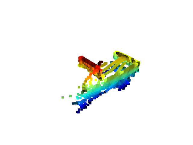
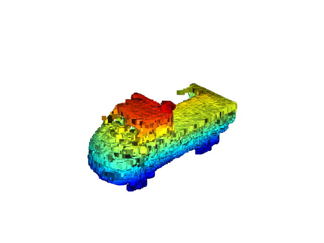
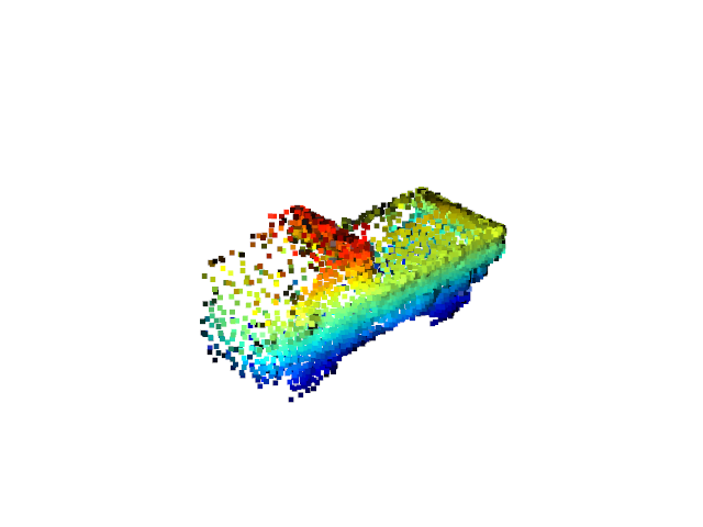
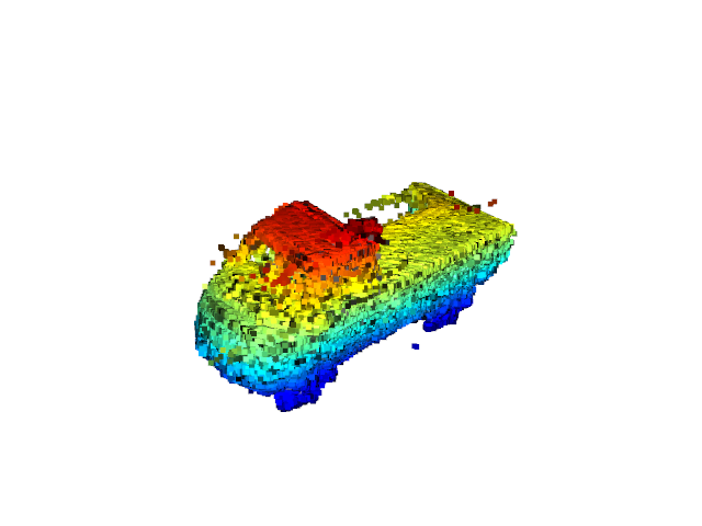
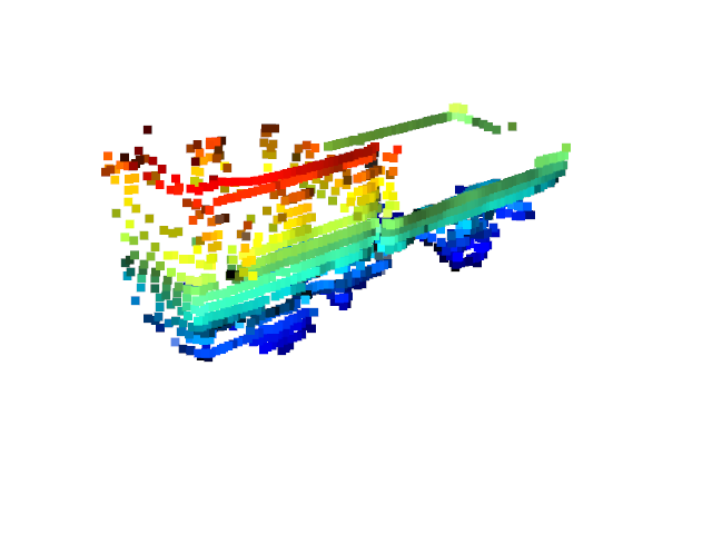
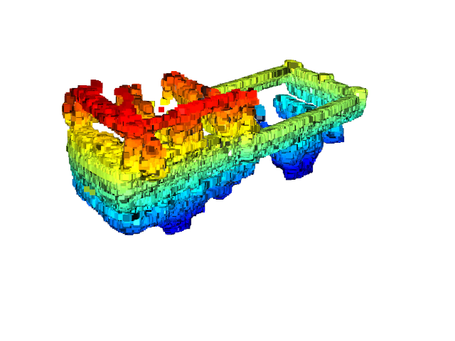
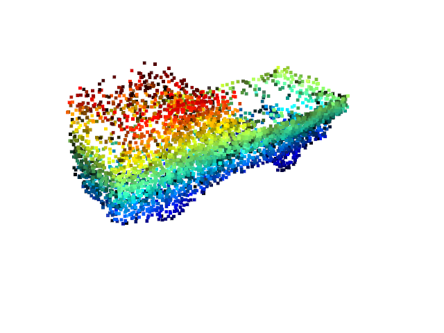
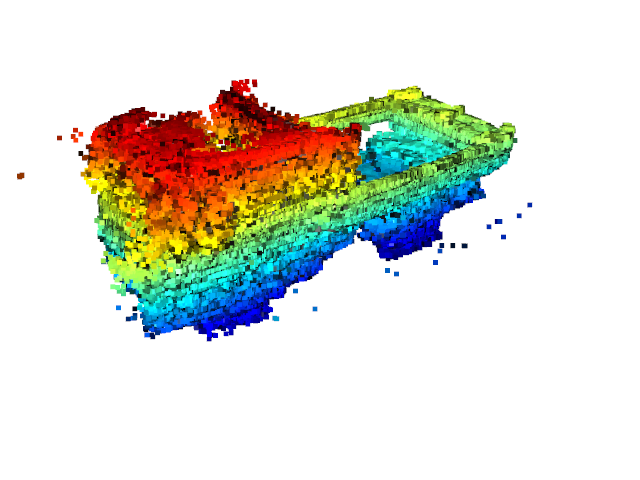
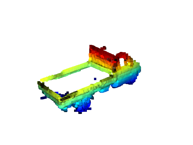
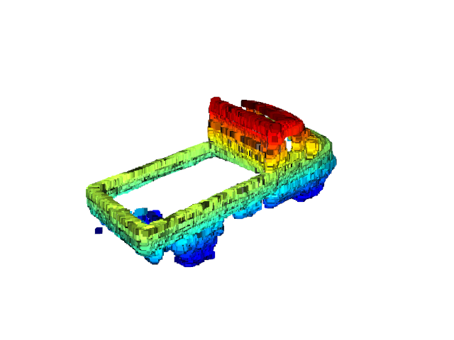
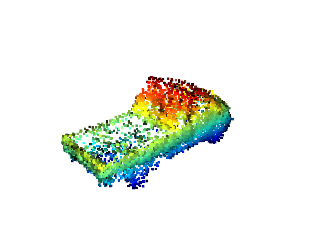
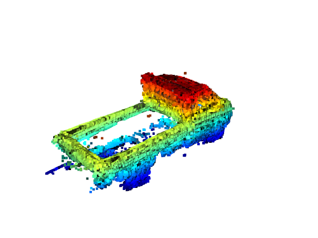
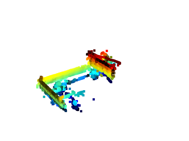
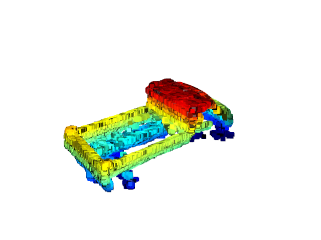
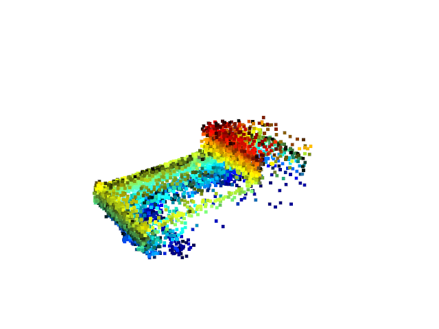
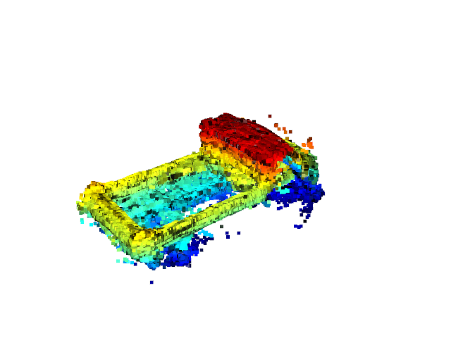
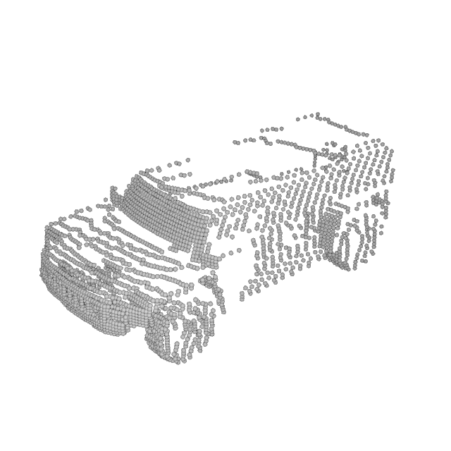
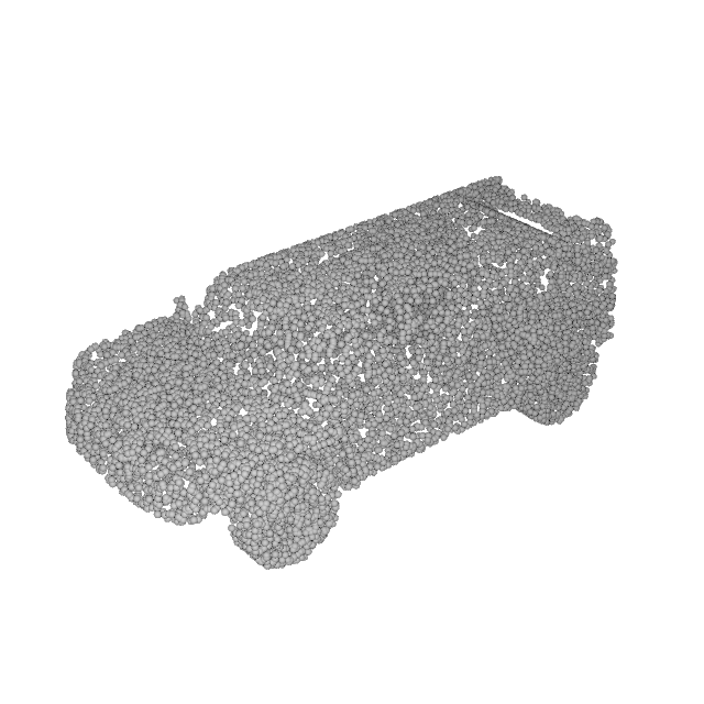
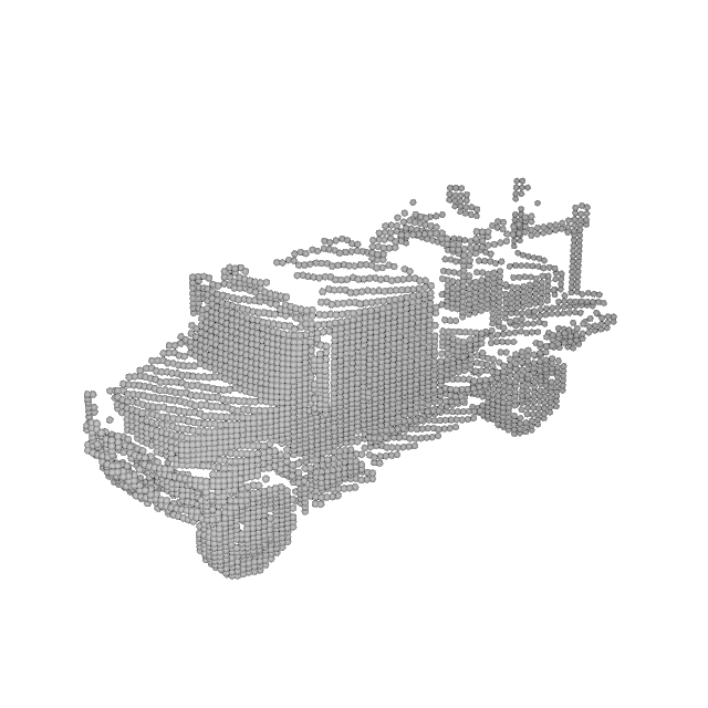
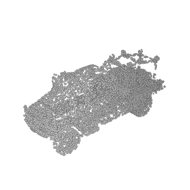
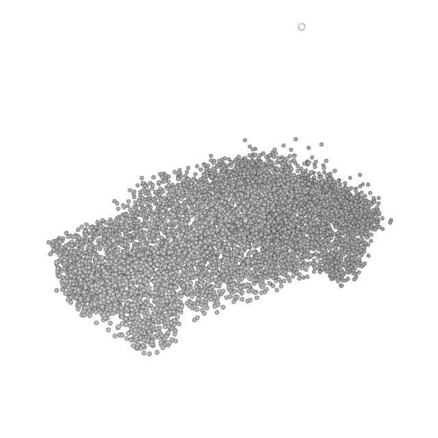
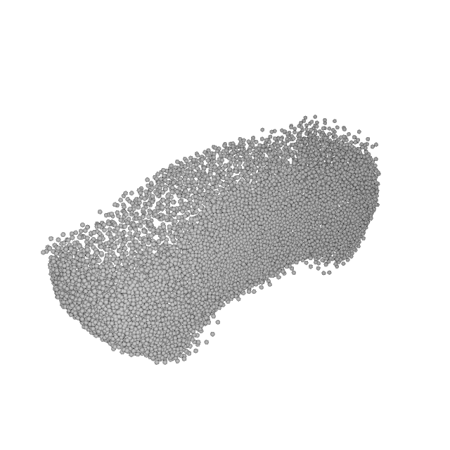
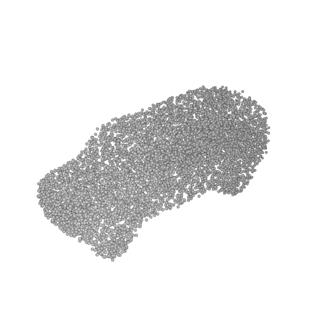
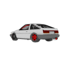
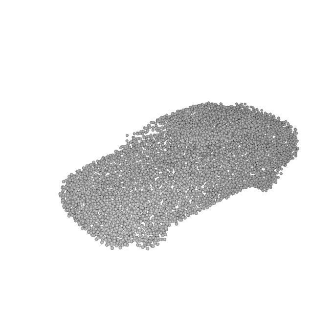
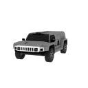
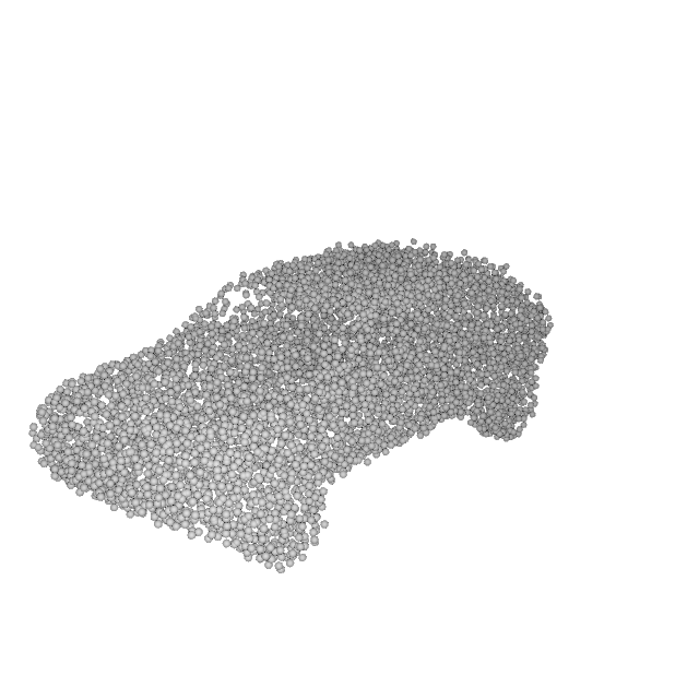
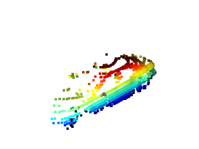
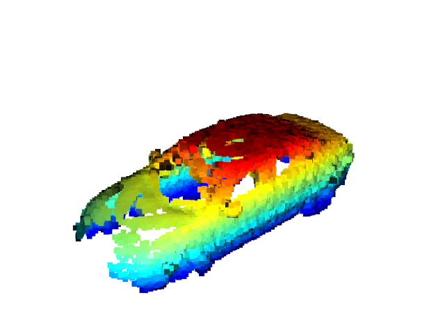
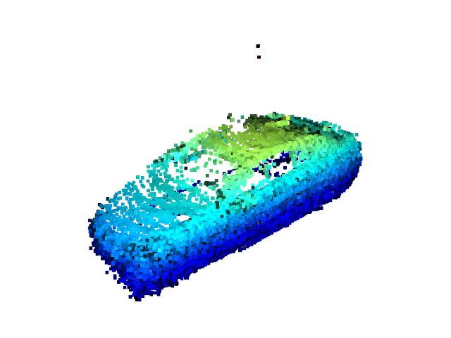
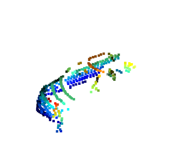
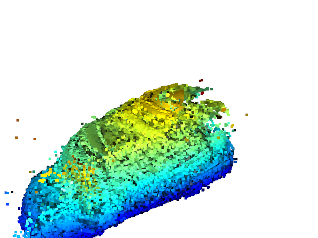
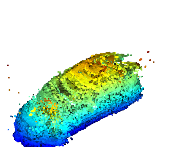
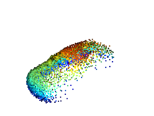
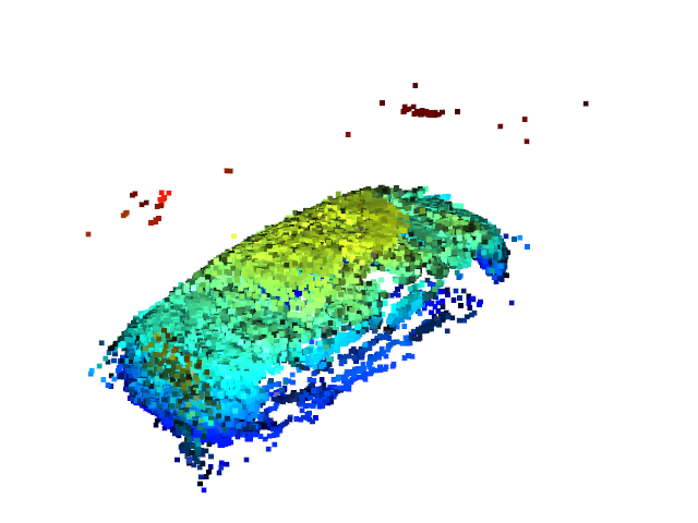
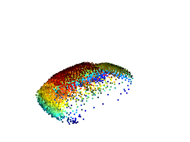
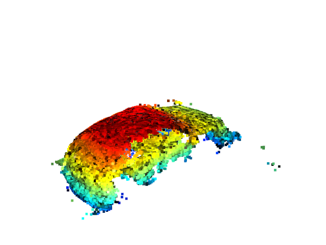
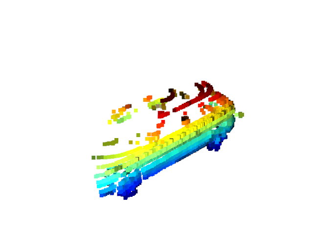
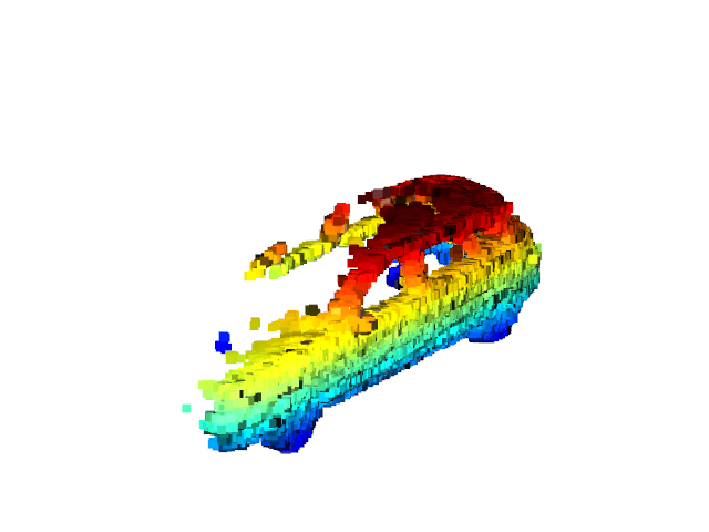
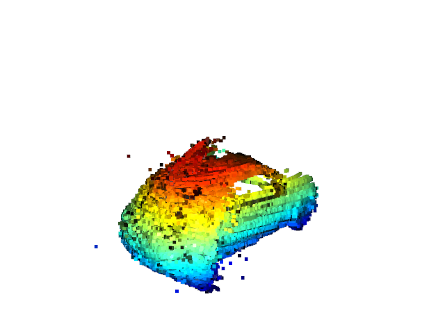
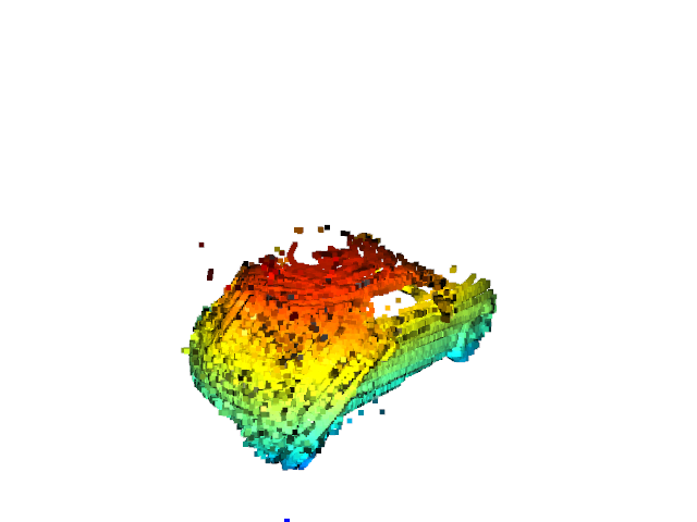
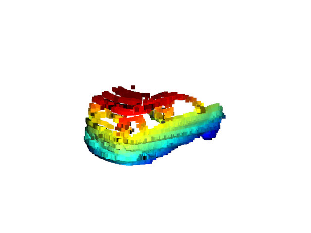
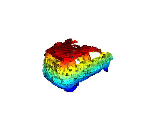
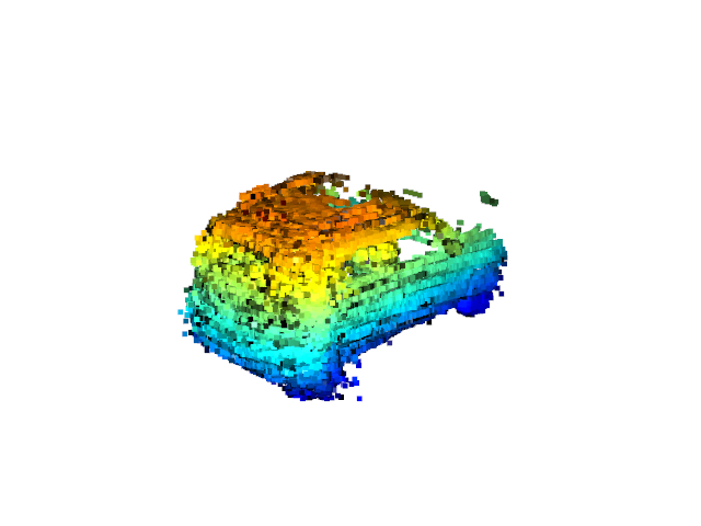
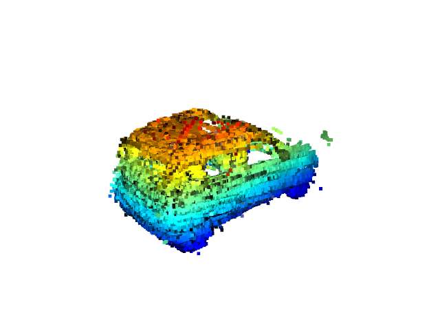
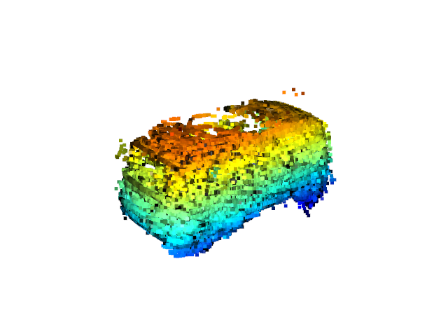
To demonstrate that our method can be applied to other categories in the wild, we experiment on parked trucks of Semantic KITTI. Due to the limited amount of data (14 valid instances), we fine-tuned the model pre-trained on our 3D vehicle dataset. The CD is 0.2942. The pose accuracy is 86.74, the median angle difference is 2.08, and the median translation MSE is 0.15. It indicates the flexibility of our method, which can be optimized during inference. Some examples are visualized in Fig 2.

5 Clarification for the GT of our 3D vehicle dataset

Note that we leverage symmetry to generate ground truth complete shapes of our 3D vehicle dataset. However, for SemanticKITTI, due to lack of GT boxes, we use the point clouds fused over frames as “partial” GT. Thus, we provide the quantitative results of shape completion on our 3D vehicle dataset evaluated by “partial” GT. The chamfer distance of our method improves from 0.255 to 0.195, while local ICP and global ICP improve from 0.315 to 0.275 and from 0.309 to 0.274 respectively. The ranking among different methods remains the same. The performance of point cloud registration is not affected.

6 More qualitative results

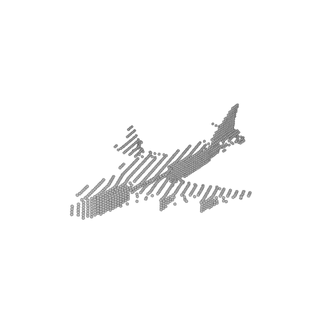
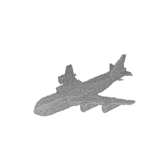
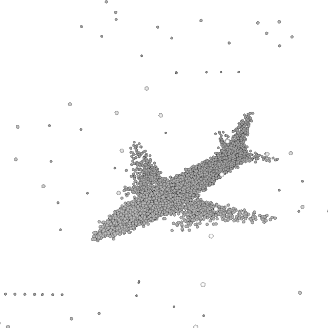
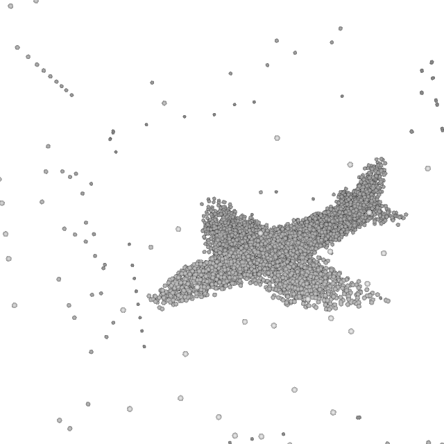
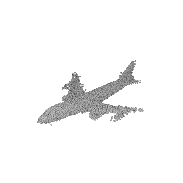
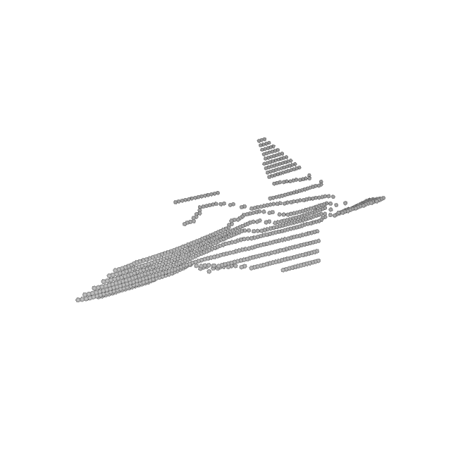
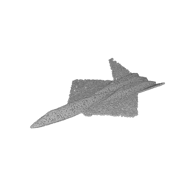
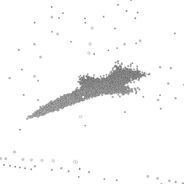
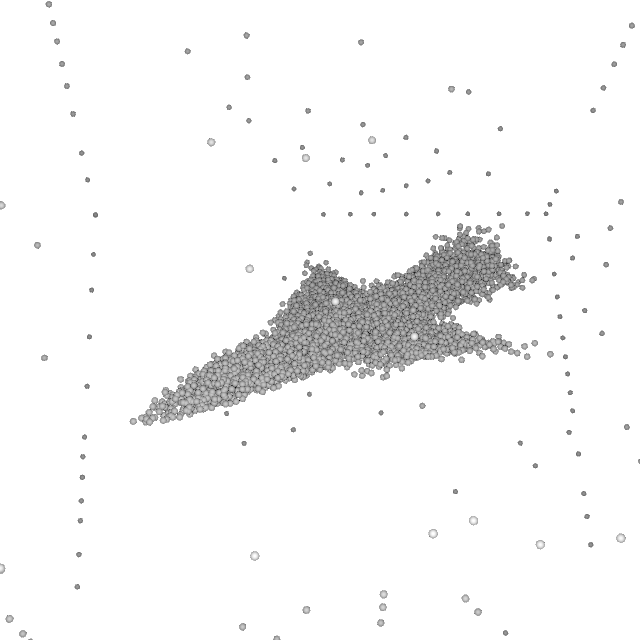
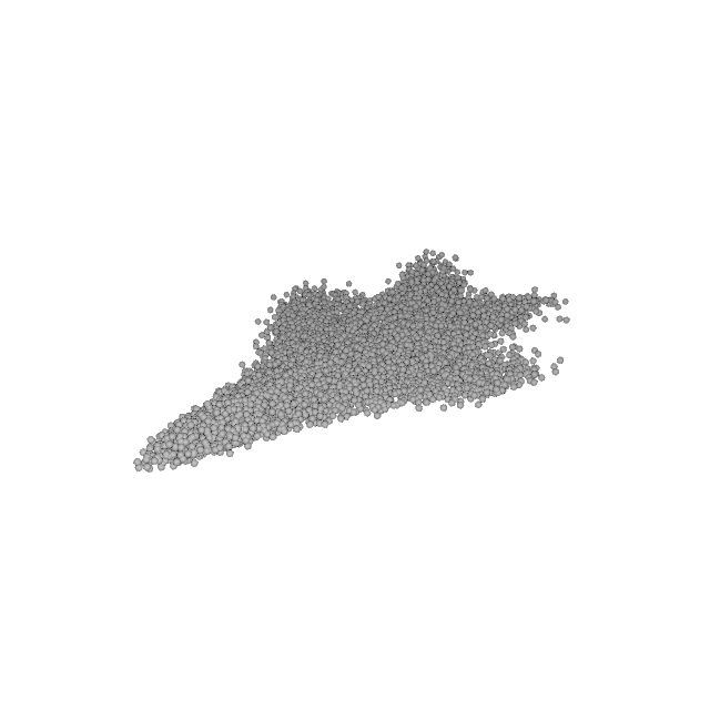
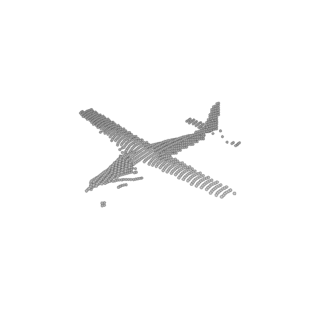
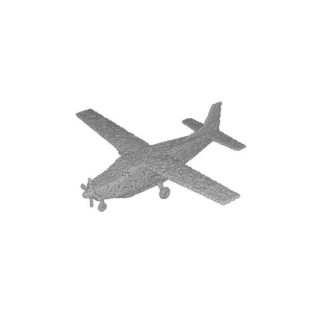
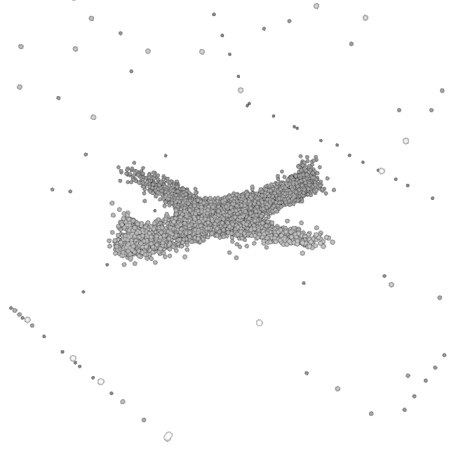
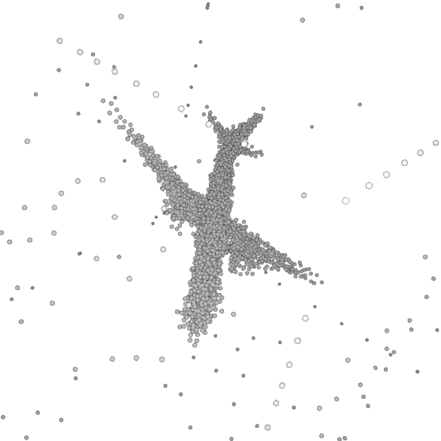
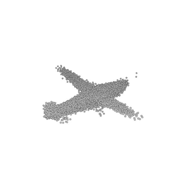
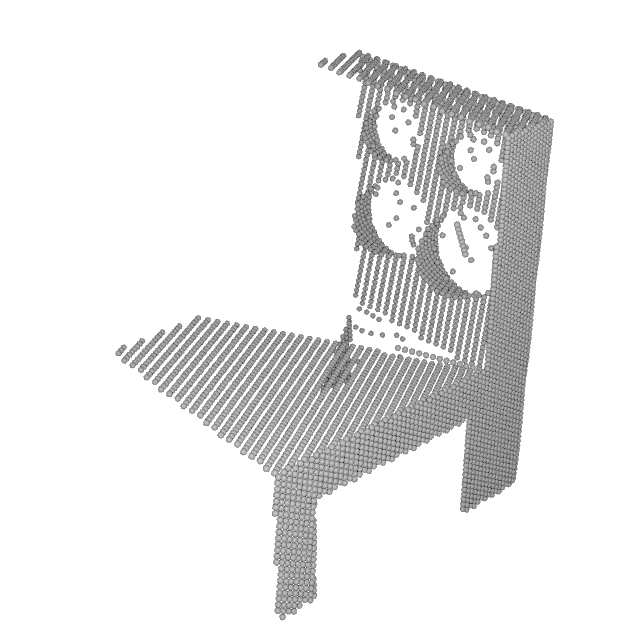
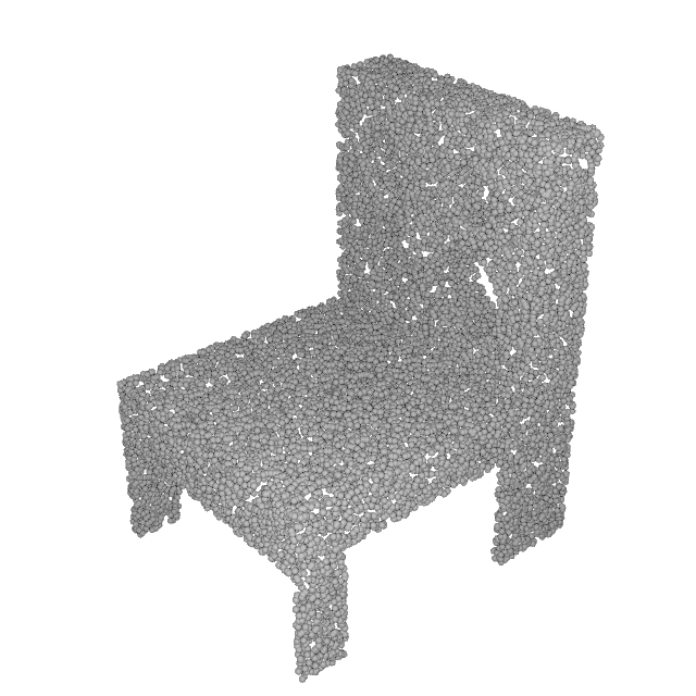
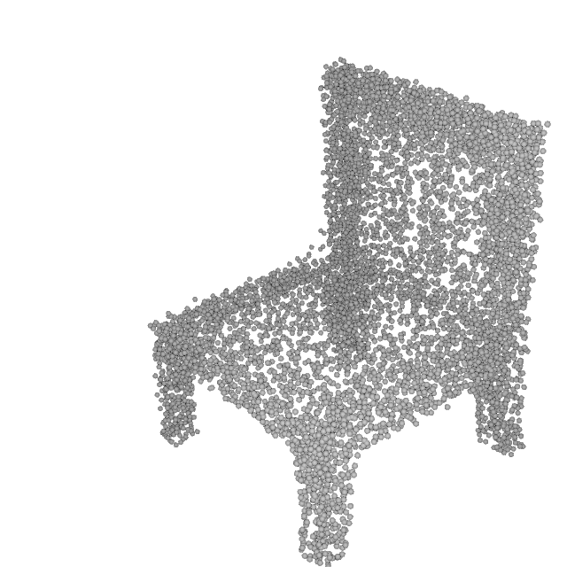
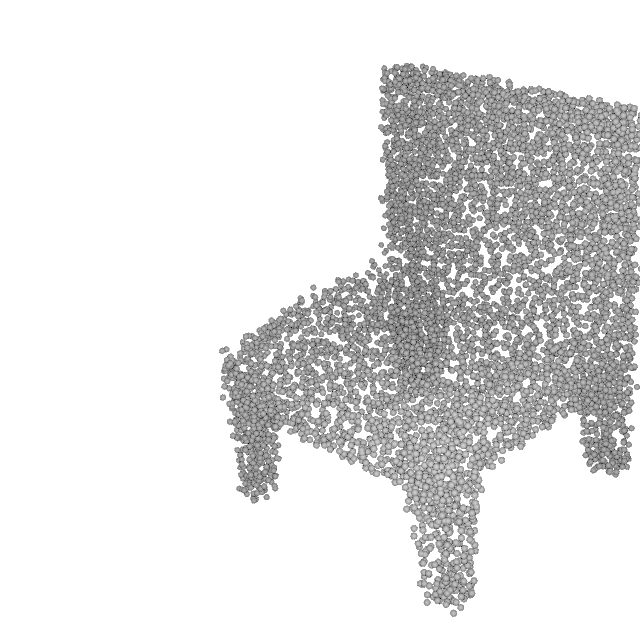
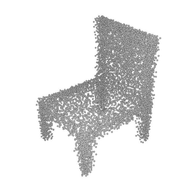
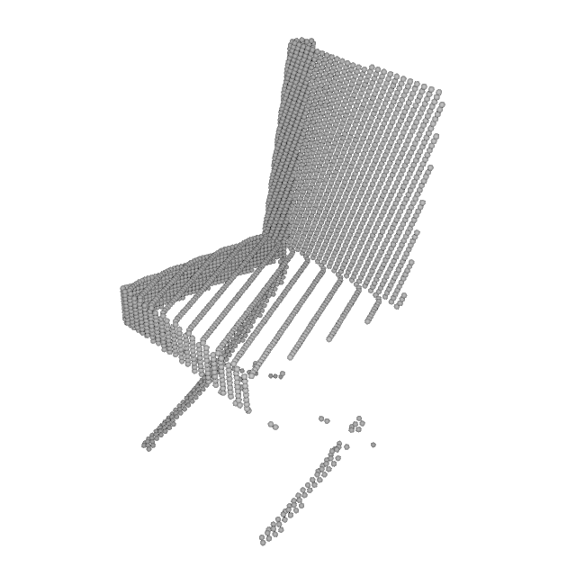
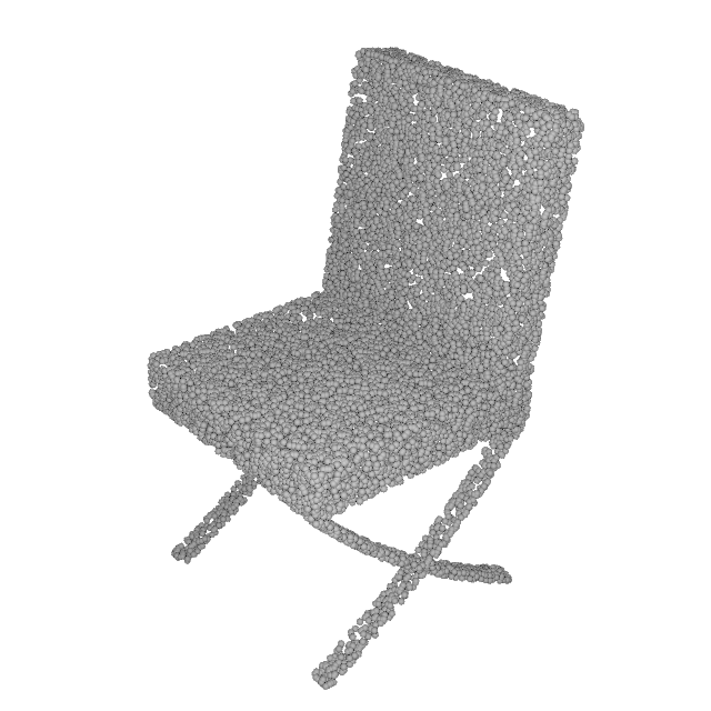
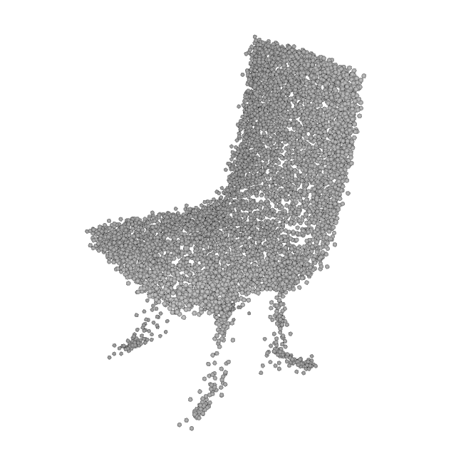
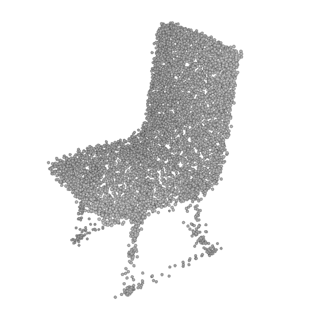
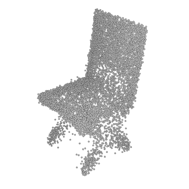
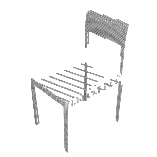
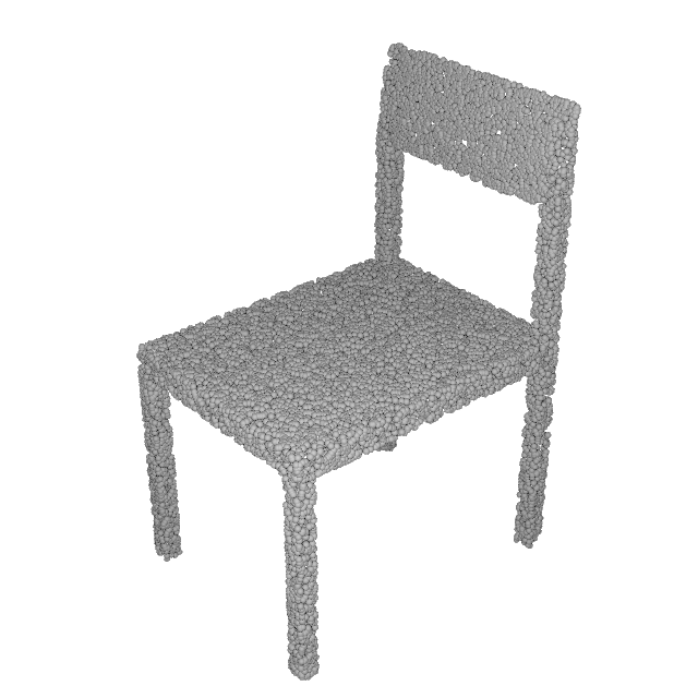
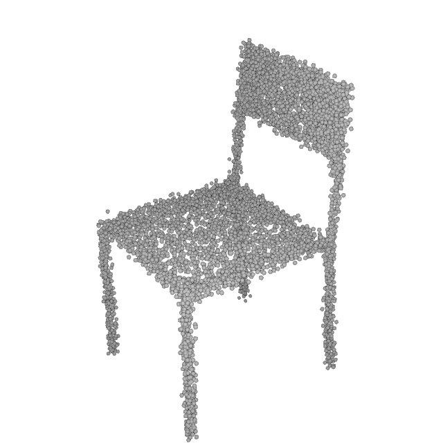
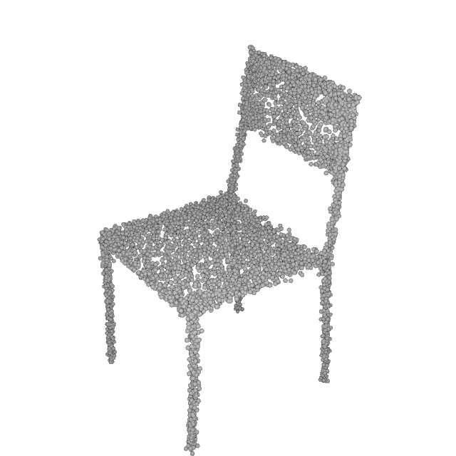
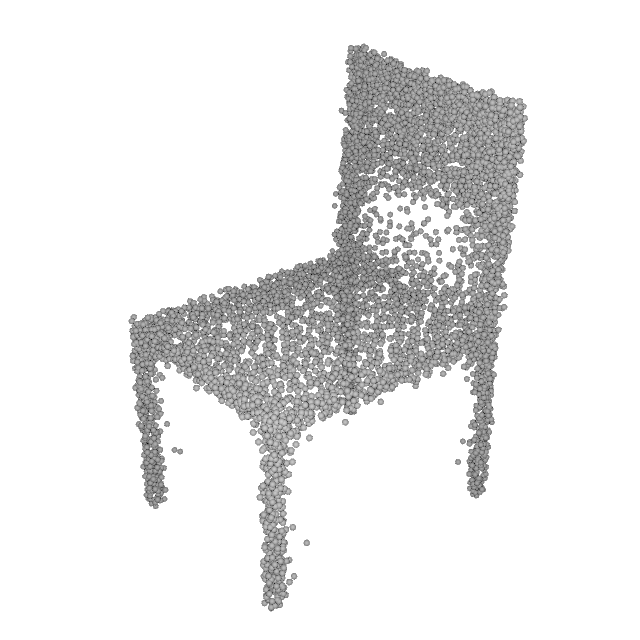
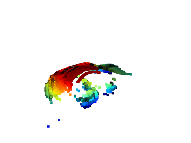
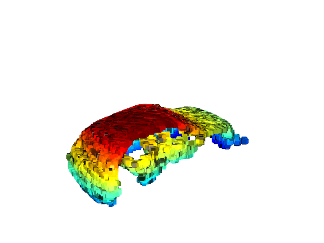
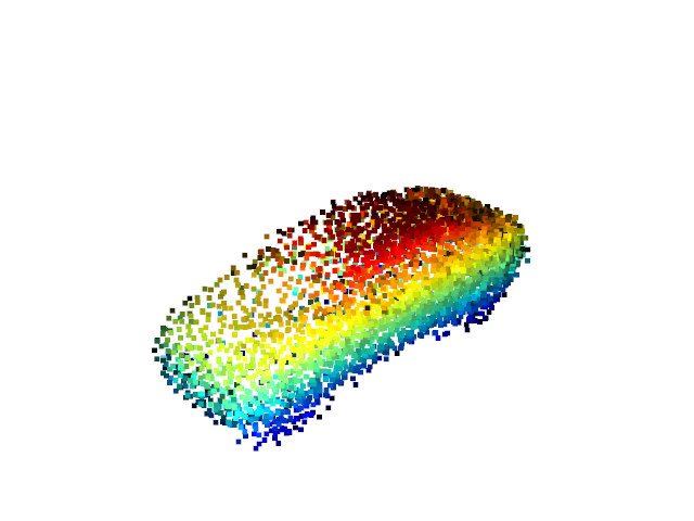
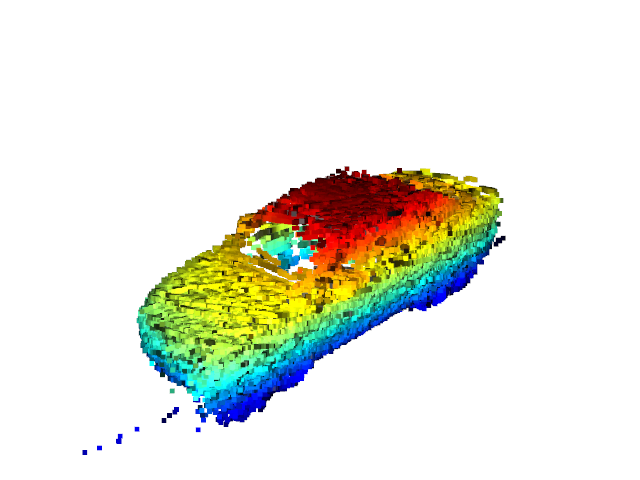
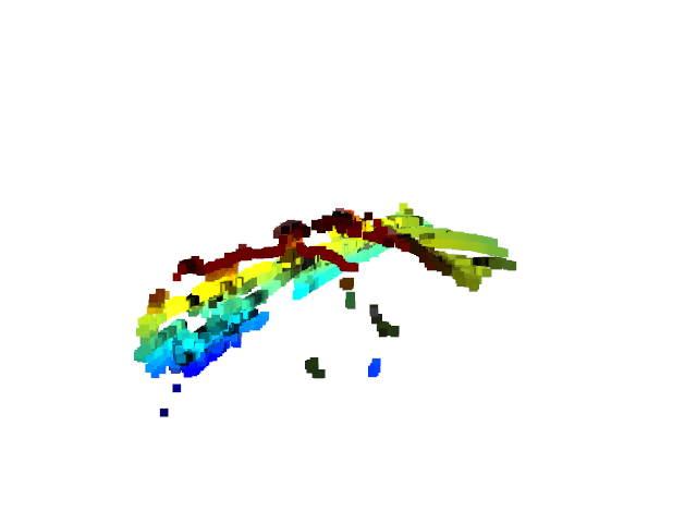
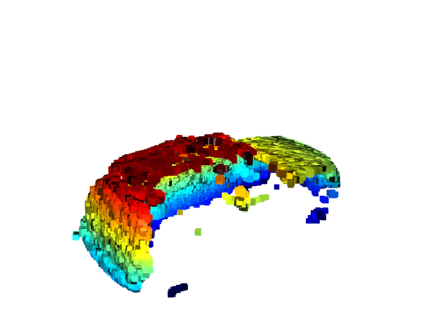
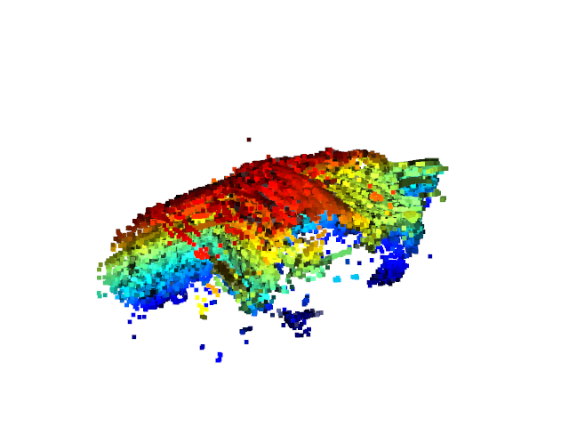
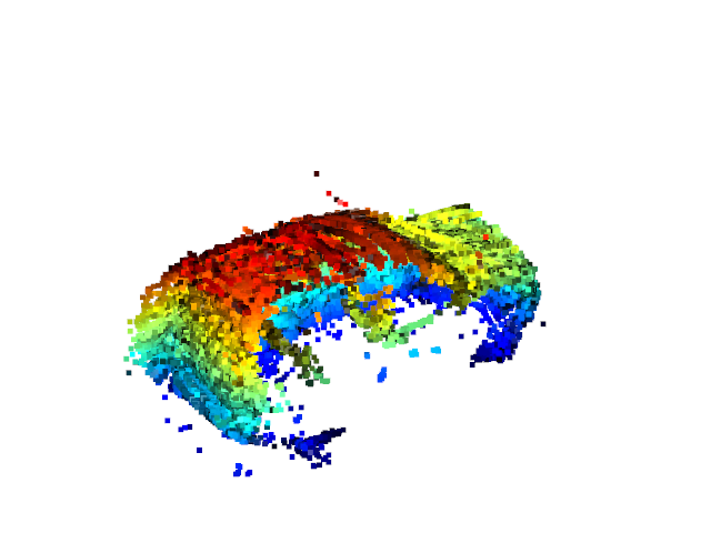
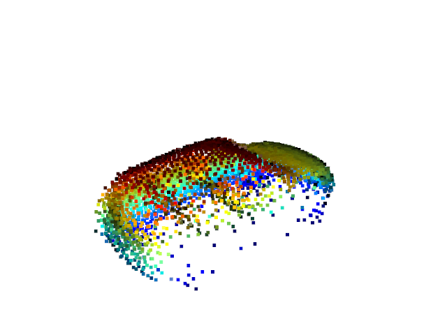
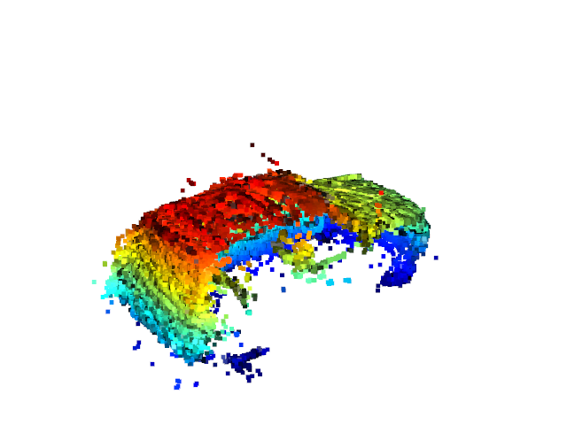
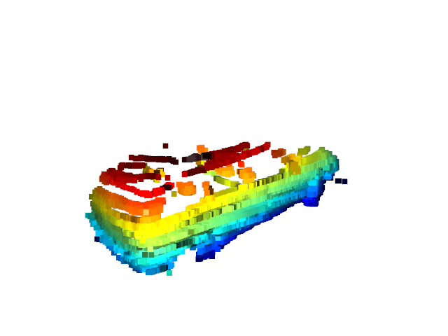
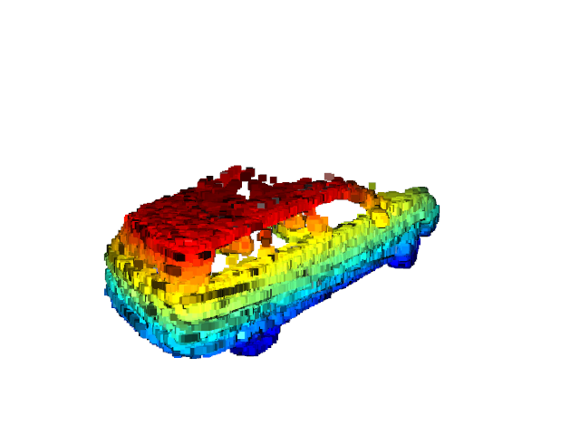
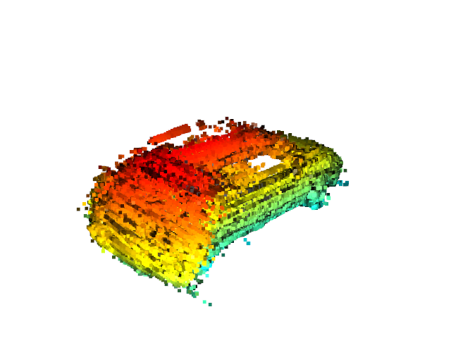
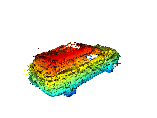
To better understand how our method performs compared to baselines, we visualize more results in this section. Fig 3 demonstrates more qualitative results on ShapeNet. It can be observed that shapes and poses estimated by our method are more accurate than DPC and DPC^†, especially for chairs and planes. Since planes are usually flat, DPC and its variant suffer from sparse 2D observations and generate many artifacts.

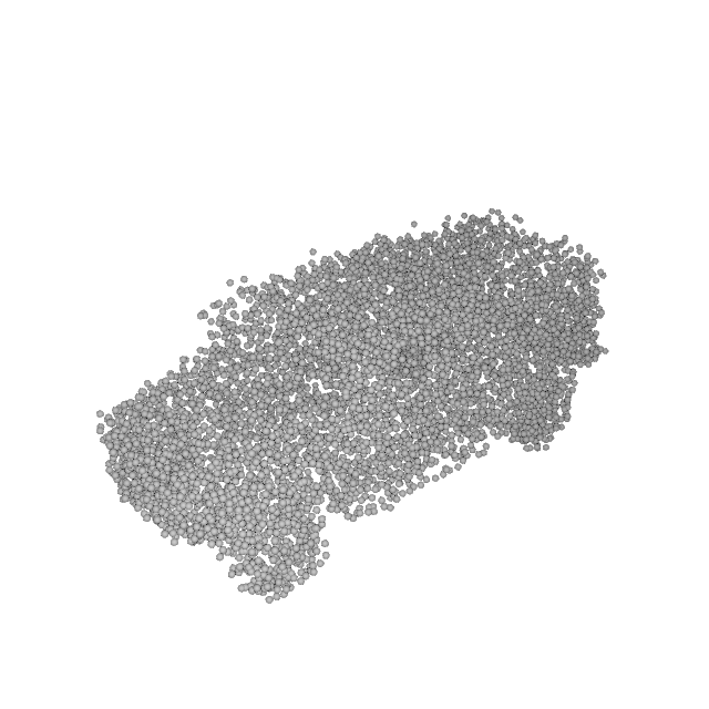
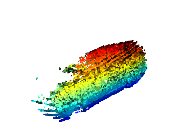
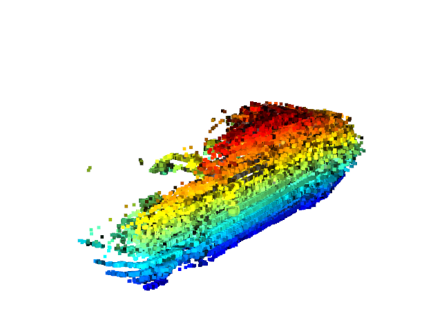
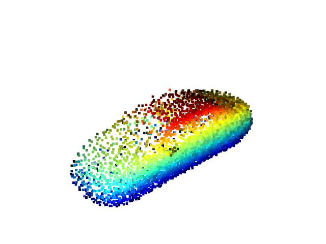
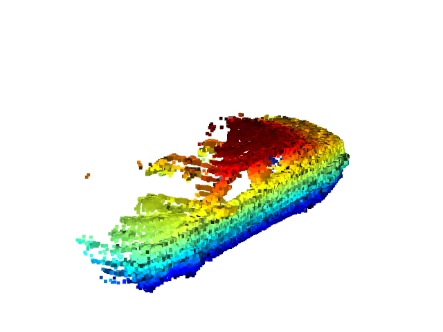
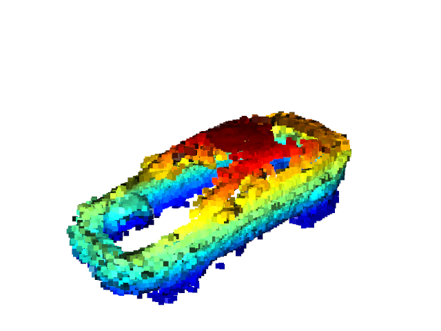
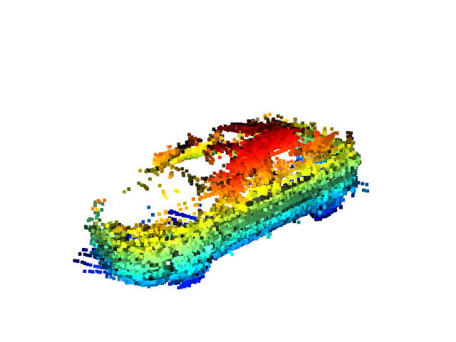
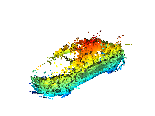
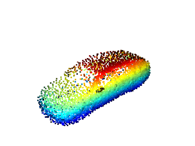
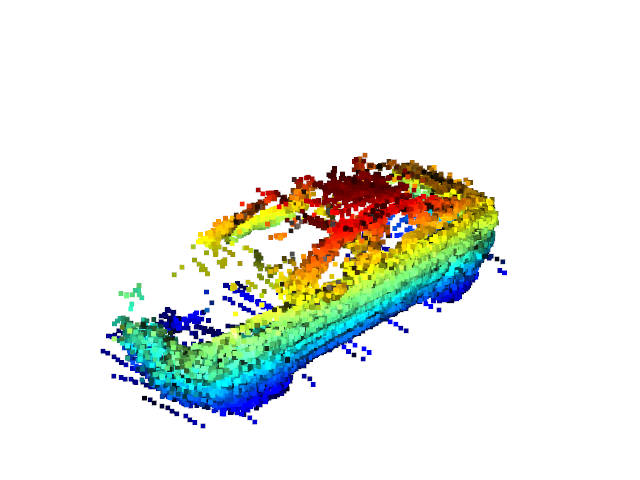
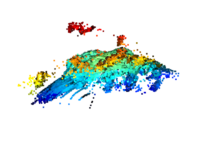
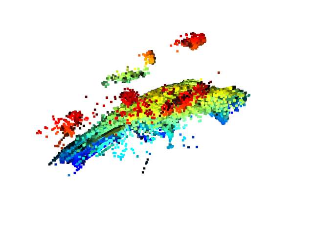
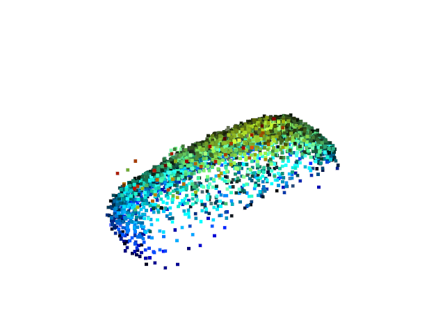
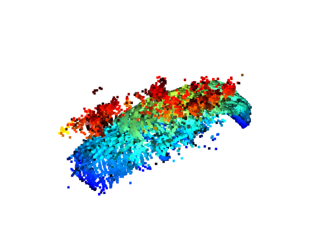
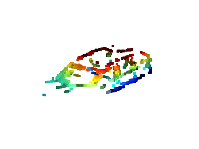
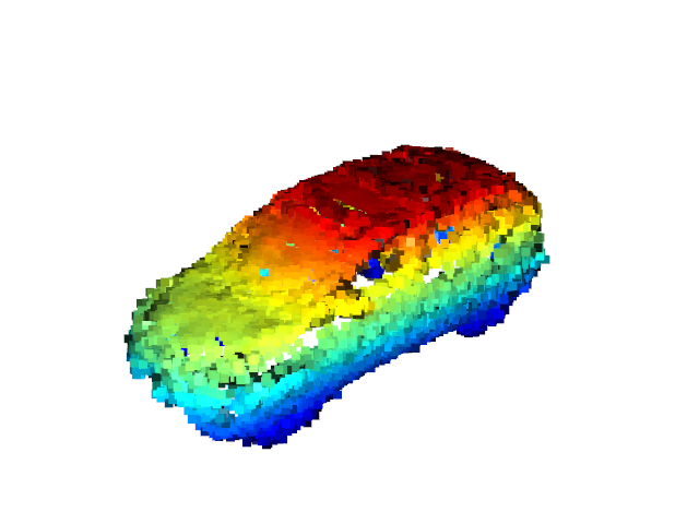
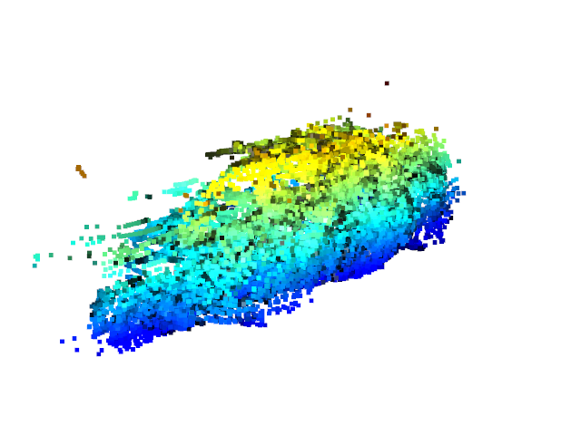
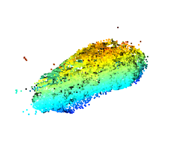
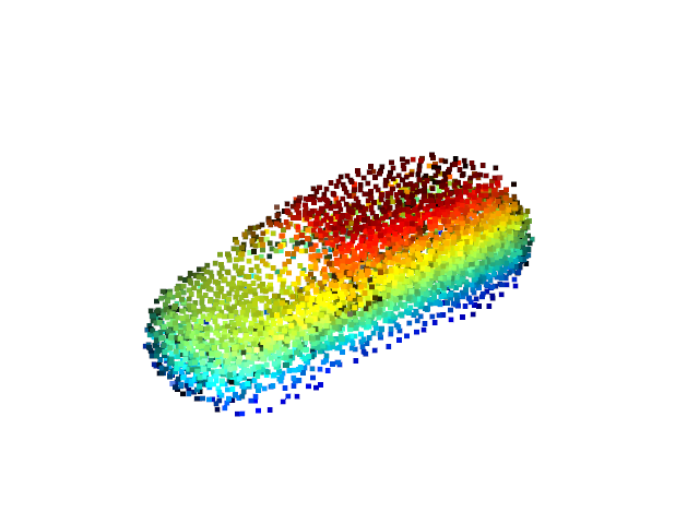
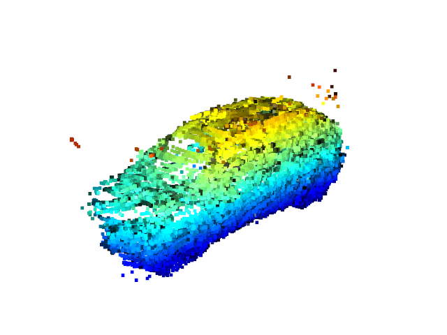
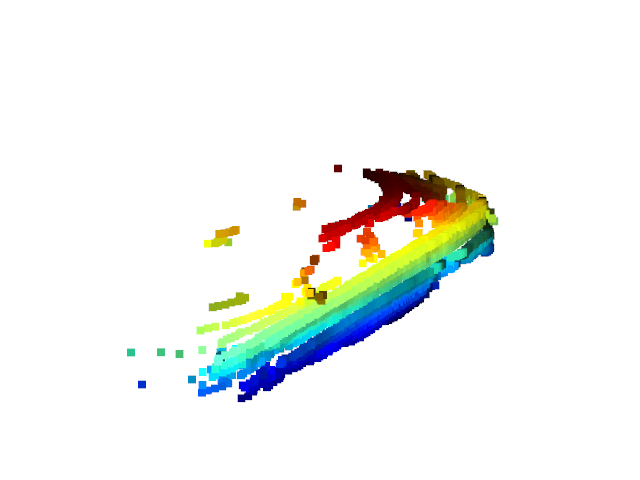
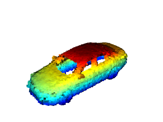
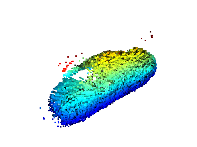
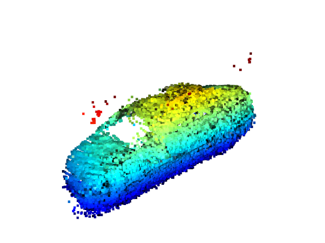
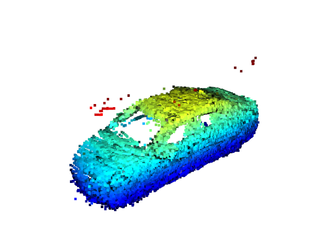
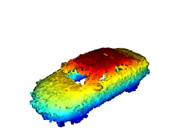
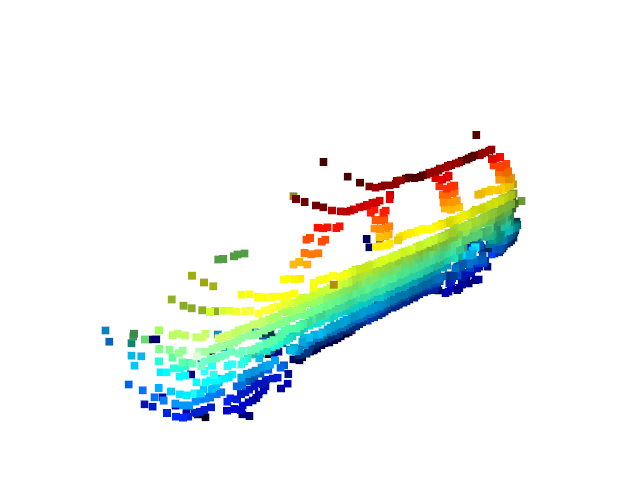
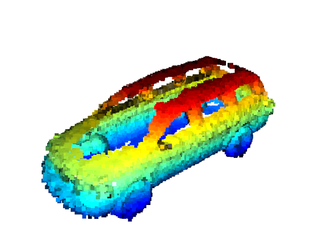
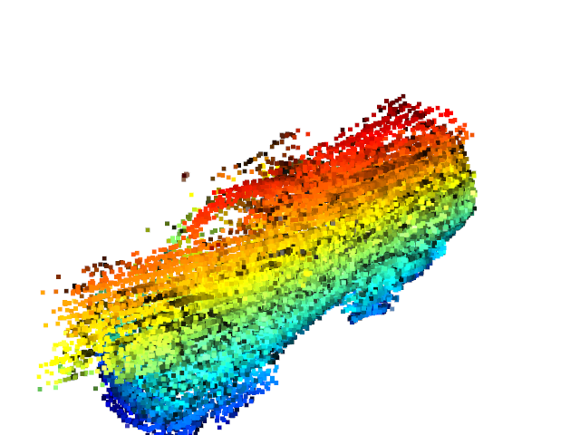
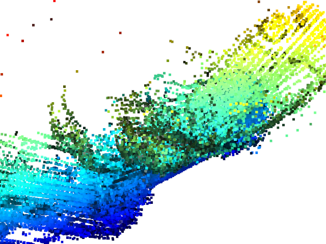
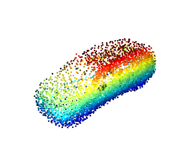
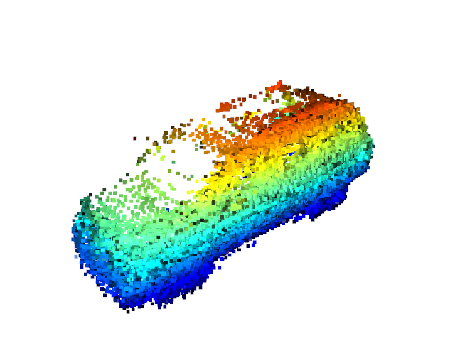
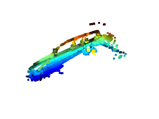
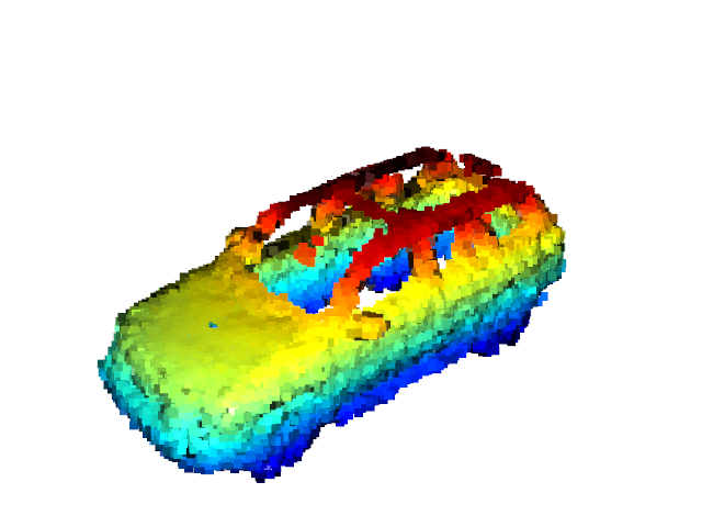
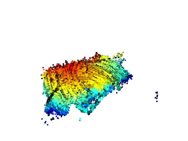
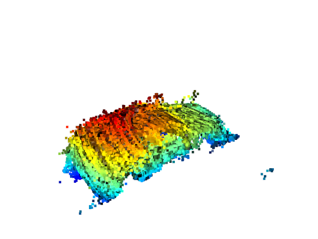
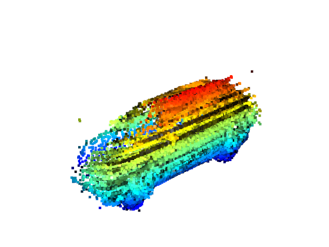
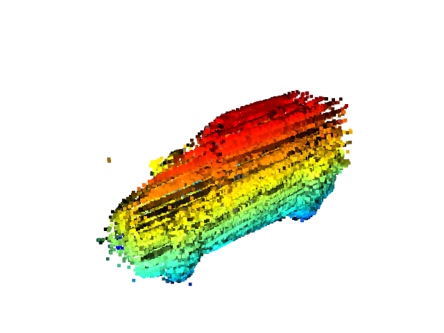
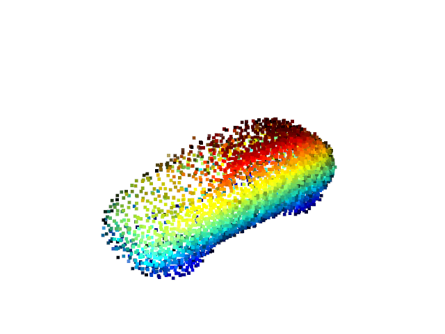
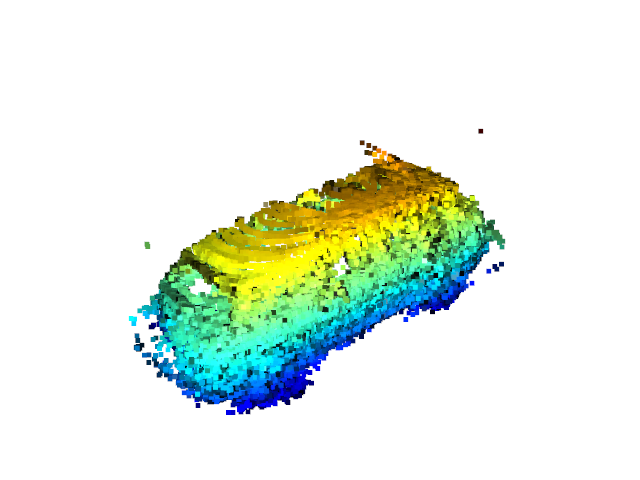
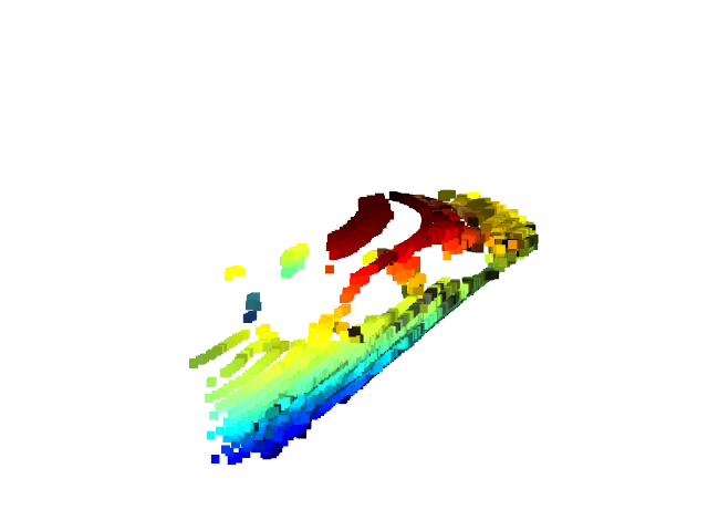
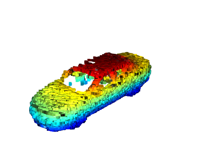
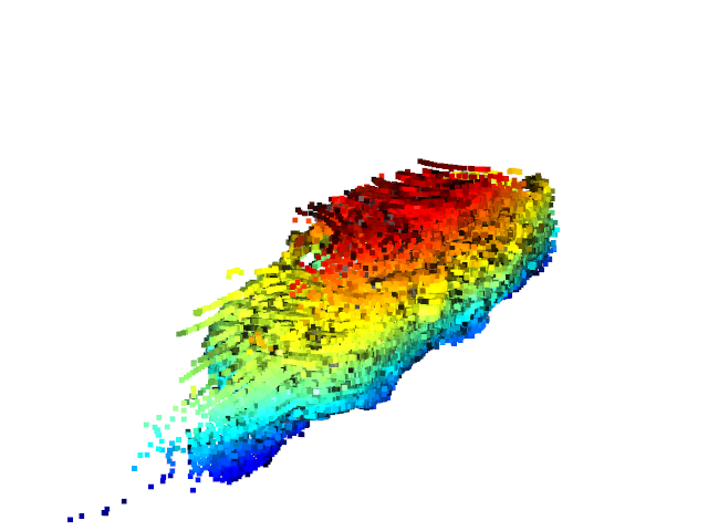
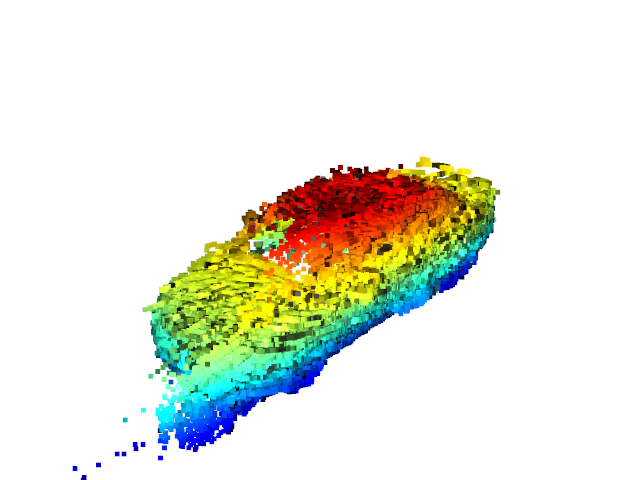
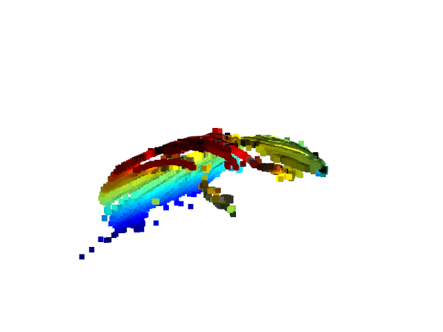
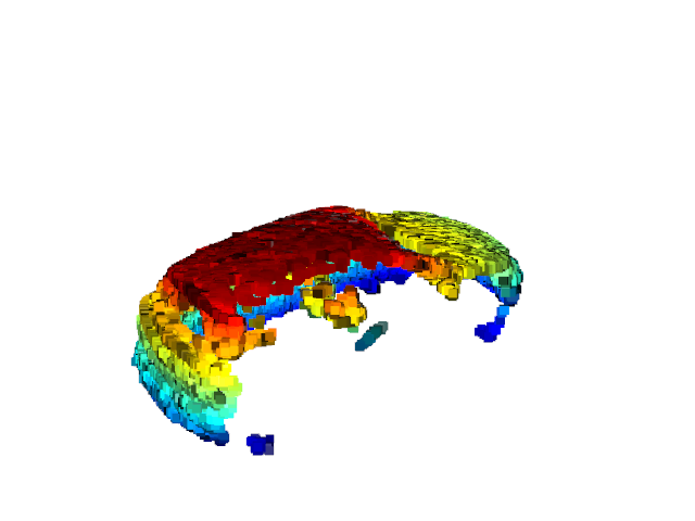
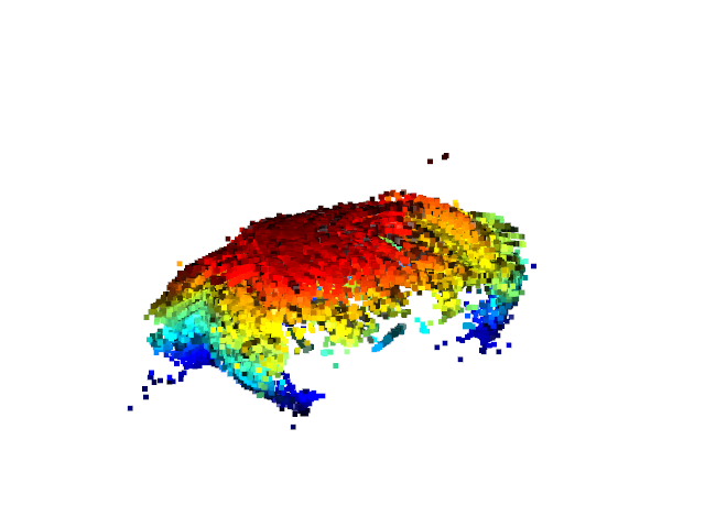
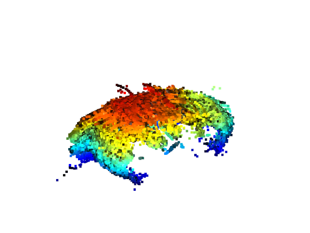
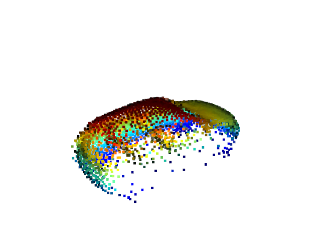
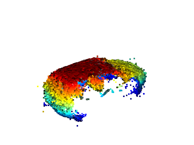
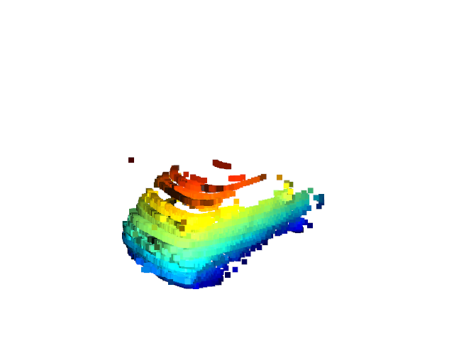
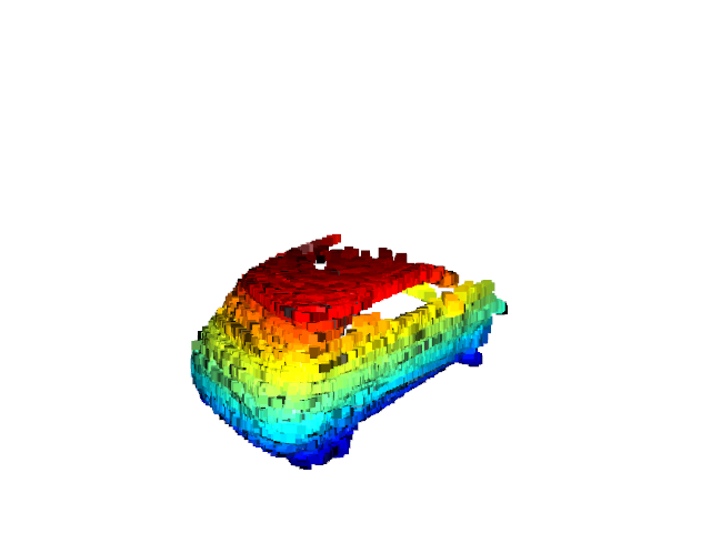
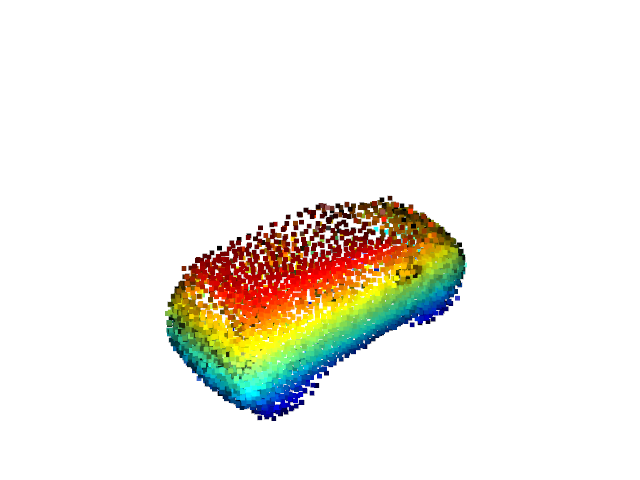
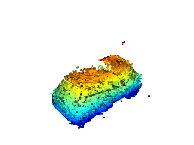
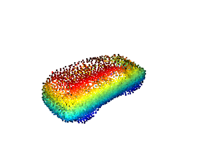
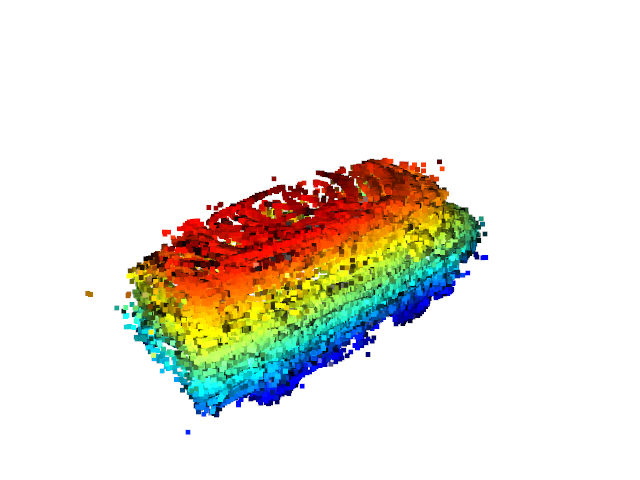
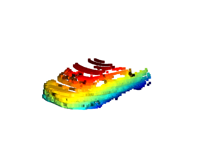
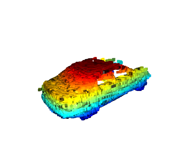
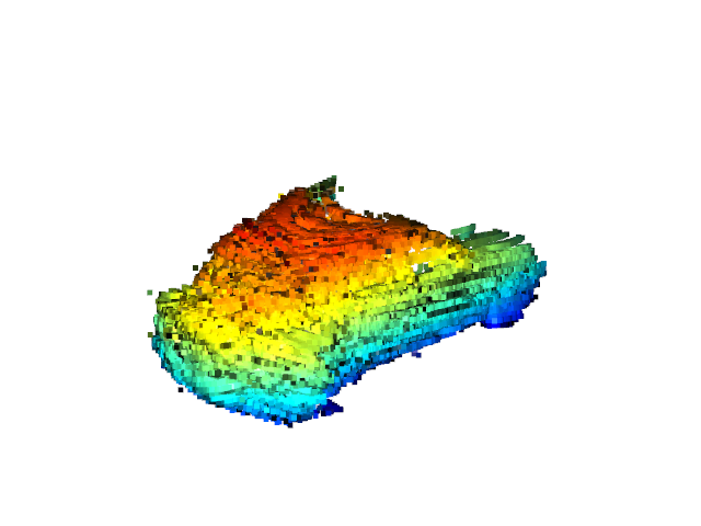
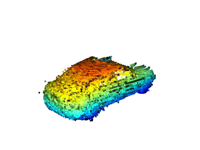
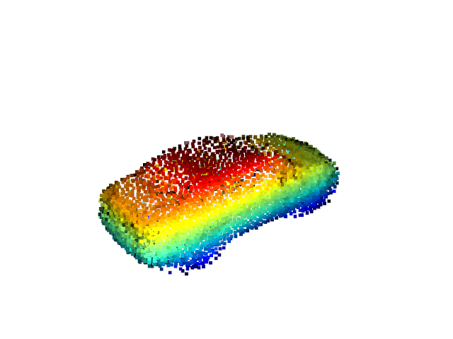
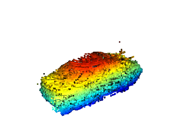
Fig 4 and Fig 5 include more qualitative results on real LiDAR datasets. Apart from shape completion, our weakly-supervised approach can be easily extended to point cloud registration. As our method estimates the 6-DoF pose of the canonical shape, we can estimate the transformation from one partial point cloud to another, by first transforming the source point cloud to the canonical frame and then to the sensor coordinate system of the target point cloud. We select the middle frame of a sequence as the target, and fuse all the partial observations in a sequence according to estimated transformations. Fused point clouds are visualized in the last column (Ours(fusion)) of Fig 4. Although the predicted complete shape of our method lacks fine details, the estimated pose is accurate, and thus the fused point cloud is very close to the ground truth. Our method outperforms ICP methods, which implies that the knowledge of the complete shape eases the challenging problem of partial point cloud registration, especially for real, sparse point clouds.

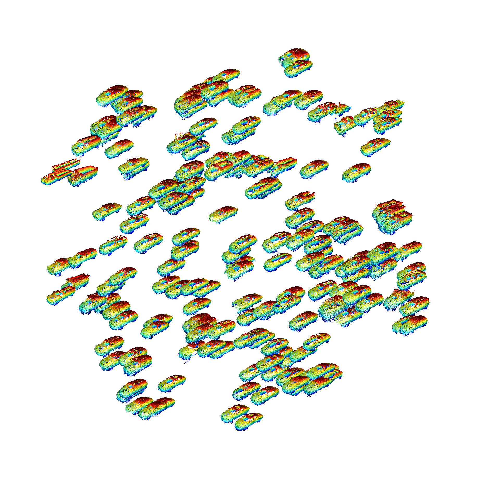
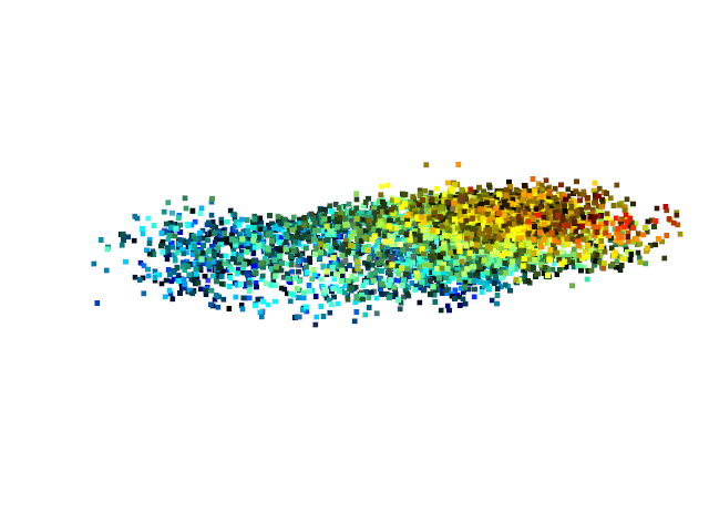
Moreover, we show t-SNE visualization of the shape features learned from our 3D vehicle dataset in Fig 6. Close features correspond to instances with similar shapes, which indicates that the learned shape features are meaningful.

Input(Ours)

Input(DPC)

GT

DPC

DPC^†

Ours

Figure 3: Qualitative results of 3D shape completion on the test set of ShapeNet. All the point clouds are transformed to the ground-truth canonical frame and visualized at a fixed viewpoint. For cars, we use the variant of our method.

Input

Ground truth

Local-ICP

Global-ICP

Ours(shape)

Ours(registration)

Figure 4: Qualitative results of our method compared against ground-truth and ICP on our 3D vehicle dataset. All the point clouds are transformed to the ground-truth canonical frame and visualized at a fixed viewpoint. We denote our approach for 3D shape completion and point cloud registration by Ours(shape) and Ours(registration).

Input

Ground truth

Local-ICP

Global-ICP

Ours(shape)

Ours(registration)

Figure 5: Qualitative results of our method compared against ground-truth and ICP on SemanticKITTI. All the point clouds are transformed to the ground-truth canonical frame and visualized at a fixed viewpoint. We denote our approach for 3D shape completion and point cloud registration by Ours(shape) and Ours(registration).

Figure 6: t-SNE visualization of the shape features learned from our 3D vehicle dataset. 200 samples from different instances are randomly chosen from the validation set. For each sample, we visualize its corresponding GT point cloud.

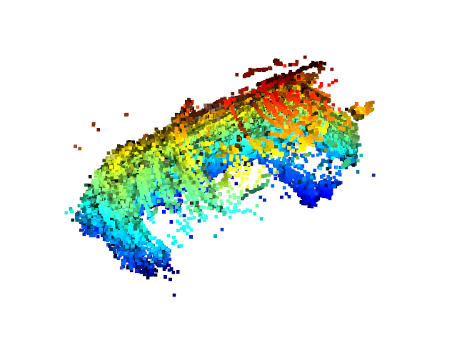
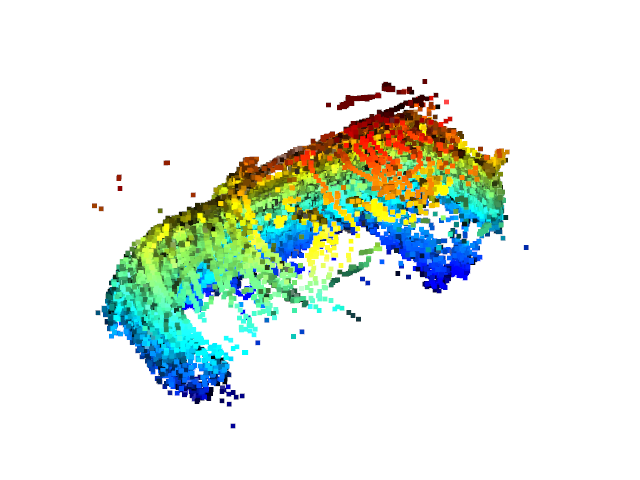
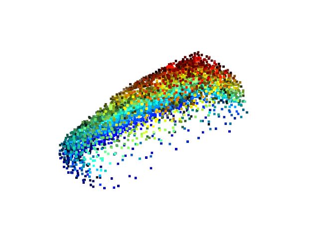
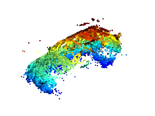
7 Sensitivity to initialization

It is intuitive that the randomness of initialization and optimization will lead to very different results for not fully-supervised approaches. Thus, we would like to investigate how sensitive our method as well as other not fully-supervised baselines are to initialization. Table 4 shows the average and standard deviation of 3 trials on ShapeNet. It is observed that our method shows a lower variance compared to DPC [1] in general. In addtion, Table 5 shows the average and standard deviation of 5 trials on real LiDAR datasets. It is worthy of future work to study how to lower the variance.

Category	Method	CD	Acc($\leq 30^{\circ}$)
Airplane	DPC	7.20 (0.81)	76.11 (1.69)
	DPC†	17.21 (3.59)	34.83 (18.07)
	Ours	1.95 (0.03)	90.87 (3.40)
Car	DPC	3.64 (0.13)	83.33 (1.26)
	DPC†	9.66 (4.31)	35.73 (40.47)
	Ours	2.66 (0.05)	49.58 (0.58)
Chair	DPC	6.24 (1.64)	57.13 (26.67)
	DPC†	7.38 (0.05)	69.46 (0.91)
	Ours	3.33 (0.002)	95.20 (0.65)

Table 4: We report the chamfer distance and the pose accuracy of 3 trials on the test set of ShapeNet. The chamfer distance is multiplied by 100. The average with the standard deviation (in the parentheses) is reported.

Dataset	CD	Acc($\leq 30^{\circ}$)	Rot $\Delta\theta$	Trans $\Delta t$
3D vehicle dataset	0.26 (0.009)	76.54 (19.20)	4.21 (1.72)	0.16 (0.032)
SemanticKITTI	0.20 (0.09)	60.62 (19.17)	11.54 (6.26)	0.21 (0.032)

Table 5: We report the chamfer distance, the pose accuracy, the median angle difference and the median translation MSE of 5 trials on the test set of real LiDAR datasets. The average with the standard deviation (in the parentheses) is reported.

8 Implementation details of DPC-LIDAR

Input

GT

DPC-LIDAR

Input

GT

DPC-LIDAR

Figure 7: Qualitative results of DPC-LIDAR on the test set of our 3D vehicle dataset. All the point clouds are transformed to the ground-truth canonical frame and visualized at a fixed viewpoint.

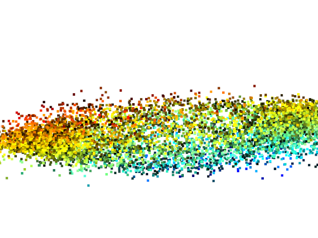
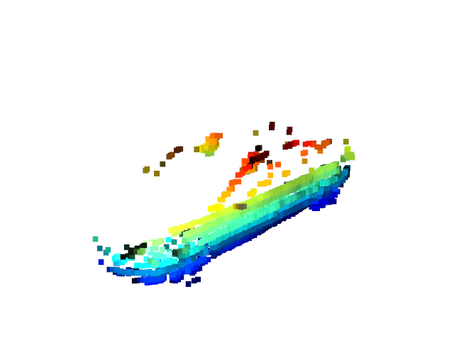
In this section, we describe more details about the implementation of the baseline DPC-LIDAR. First, We adapt DPC [1] to range images by replacing perspective transformation with polar transformation. Different from synthetic data, real data is not normalized and the distance between the partial point cloud and the sensor varies significantly (e.g. 5-30 meters). However, the camera distance is constant for the original DPC. Other weakly-supervised approaches, like MVC [2], also assume little or no translation in relative pose. Thus, we then scale the canonical shape predicted by DPC in a unit cube to the real world dimensions. The factor is selected as 6.0, as the average length of vehicles is about 5 meters. In addition, a radial offset, which is the average of the maximum and the minimum radial distances of the partial point cloud, is provided. The range image provided as input to DPC is generated directly from the input partial point cloud that we take as input for our approach. The resolution is $128\times 128$. However, DPC-LIDAR performs poorly on real data, even with these modifications. Fig 7 showcases some examples of DPC-LIDAR on our 3D vehicle dataset.

References

- [1] Insafutdinov, E., Dosovitskiy, A.: Unsupervised learning of shape and pose with differentiable point clouds. In: Advances in Neural Information Processing Systems. pp. 2802–2812 (2018)
- [2] Tulsiani, S., Efros, A.A., Malik, J.: Multi-view consistency as supervisory signal for learning shape and pose prediction. In: Proceedings of the IEEE Conference on Computer Vision and Pattern Recognition. pp. 2897–2905 (2018)