Optimal Combination of Linear and Spectral Estimators for Generalized Linear Models
Abstract
We study the problem of recovering an unknown signal given measurements obtained from a generalized linear model with a Gaussian sensing matrix. Two popular solutions are based on a linear estimator and a spectral estimator . The former is a data-dependent linear combination of the columns of the measurement matrix, and its analysis is quite simple. The latter is the principal eigenvector of a data-dependent matrix, and a recent line of work has studied its performance. In this paper, we show how to optimally combine and . At the heart of our analysis is the exact characterization of the empirical joint distribution of in the high-dimensional limit. This allows us to compute the Bayes-optimal combination of and , given the limiting distribution of the signal . When the distribution of the signal is Gaussian, then the Bayes-optimal combination has the form and we derive the optimal combination coefficient. In order to establish the limiting distribution of , we design and analyze an Approximate Message Passing (AMP) algorithm whose iterates give and approach . Numerical simulations demonstrate the improvement of the proposed combination with respect to the two methods considered separately.
1 Introduction
In a generalized linear model (GLM) [NW72, McC18], we want to recover a -dimensional signal given i.i.d. measurements of the form:
| (1.1) |
where denotes the scalar product, are known sensing vectors, and the (stochastic) output function is a known probability distribution. GLMs arise in several problems in statistical inference and signal processing. Examples include photon-limited imaging [UE88, YLSV12], compressed sensing [EK12], signal recovery from quantized measurements [RG01, BB08], phase retrieval [Fie82, SEC+15], and neural networks with one hidden layer [LBH15].
The problem of estimating from is, in general, non-convex, and semi-definite programming relaxations have been proposed [CESV15, CSV13, WdM15, TR19]. However, the computational complexity and memory requirement of these approaches quickly grow with the dimension . For this reason, several non-convex approaches have been developed, e.g., alternating minimization [NJS13], approximate message passing (AMP) [DMM09, Ran11, SR14], Wirtinger Flow [CLS15], Kaczmarz methods [Wei15], and iterative convex-programming relaxations [BB08, BR17, GS18, DTL18]. The Bayes-optimal estimation and generalization error have also been studied in [BKM+19]. When the output function is unknown, (1.1) is called the single-index model in the statistics literature, see e.g. [Bri82, LD89, KKSK11]. The problem of recovering a structured signal (e.g., sparse, low-rank) from high-dimensional single-index measurements has been an active research topic over the past few years [YWCL15, PVY17, PV16, TAH15, NLC16, Gen17, GMW18, GJ19, TR19].
Throughout this paper, the performance of an estimator will be measured by its normalized correlation (or “overlap”) with :
| (1.2) |
where denotes the Euclidean norm of a vector.
Most of the existing techniques require an initial estimate of the signal, which can then be refined via a local algorithm. Here, we focus on two popular methods: a linear estimator and a spectral estimator. The linear estimator has the form:
| (1.3) |
where denotes a given preprocessing function. The performance analysis of this estimator is quite simple, see e.g. Proposition 1 in [PVY17] or Section 2.3 of this paper. The spectral estimator consists in the principal eigenvector of a matrix of the form:
| (1.4) |
where is another preprocessing function. The idea of a spectral method first appeared in [Li92] and, for the special case of phase retrieval, a series of works has provided more and more refined performance bounds [NJS13, CSV13, CC15]. Recently, an exact high-dimensional analysis of the spectral method for generalized linear models with Gaussian sensing vectors has been carried out in [LL19, MM19]. These works consider a regime where both and grow large at a fixed proportional rate . The choice of which minimizes the value of (and, consequently, the amount of data) necessary to achieve a strictly positive scalar product (1.2) was obtained in [MM19]. Furthermore, the choice of which maximizes the correlation between and for any given value of the sampling ratio was obtained in [LAL19]. The case in which the sensing vectors are obtained by picking columns from a Haar matrix is tackled in [DBMM20].
In short, the performance of the linear estimate and the spectral estimate is well understood, and there is no clear winner between the two. In fact, the superiority of one method over the other depends on the output function and on the sampling ratio . For example, for phase retrieval (), the spectral estimate provides positive correlation with the ground-truth signal as long as [MM19], while linear estimators of the form (1.3) are not effective for any . On the contrary, for 1-bit compressed sensing () the situation is the opposite: the spectral estimator is uncorrelated with the signal for any , while the linear estimate works well. For many cases of practical interest, e.g. neural networks with ReLU activation function (), both the linear and the spectral method give estimator with non-zero correlation. Thus, a natural question is the following:
What is the optimal way to combine the linear estimator and the spectral estimator ?
This paper closes the gap and answers the question above for Gaussian sensing vectors . Our main technical contribution is to provide an exact high-dimensional characterization of the joint empirical distribution of in the limit with a fixed sampling ratio (see Theorem 1). In particular, we prove that the conditional distribution of given converges to the law of a bivariate Gaussian whose mean vector and covariance matrix are specified in terms of the preprocessing functions and . As a consequence, we are able to compute the Bayes-optimal combination of and for any given prior distribution on (see Theorem 2). In the special case in which the signal prior is Gaussian, the Bayes-optimal combination has the form , with , and we compute the optimal combination coefficient that maximizes the normalized correlation in (1.2) (see Corollary 3.4).
The characterization of the joint empirical distribution of is achieved by designing and analyzing a suitable approximate message passing (AMP) algorithm. AMP is a family of iterative algorithms that has been applied to several high-dimensional statistical estimation problems including estimation in linear models [DMM09, BM11, BM12, KMS+12], generalized linear models [Ran11, SR14, SC19], and low-rank matrix estimation [DM14, RFG09, LKZ17, MV21]. An appealing feature of AMP algorithms is that under suitable conditions on the model, the empirical joint distribution of the iterates can be exactly characterized in the high-dimensional limit, in terms of a simple scalar recursion called state evolution.
In this paper, we design an AMP algorithm that is equivalent to a power method computing the principal eigenvector of the matrix (1.4). Then, the state evolution analysis leads to the desired joint empirical distribution of . Using the limiting distribution, we reduce the vector problem of estimating given two (correlated) observations to the scalar problem of estimating the random variable given two (correlated) observations . We emphasize that the focus of this work is not on using the AMP algorithm as an estimator for the generalized linear model. Rather, we use AMP as a proof technique to characterize the joint empirical distribution of , and thereby understand how to optimally combine the two simple estimators.
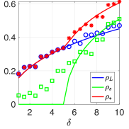
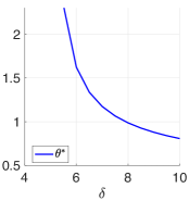
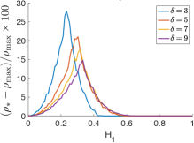
Our proposed combination of the linear and spectral estimators can significantly boost the correlation with the ground-truth signal (1.2). As an illustration, in Figure 1(a) we compare against each other the correlations and of the linear, spectral and optimal combined estimators, respectively, for a range of values of the sampling ratio and measurements of the form . Here, is uniformly distributed on the -dimensional sphere of radius , , , and the preprocessing functions are chosen as follows: and . The solid lines correspond to analytically derived asymptotic formulae, and they are compared against numerical simulations (cf. markers of the corresponding color) computed for . Specifically, the red line corresponds to the optimal combined estimator (in this example, the empirical distribution of is Gaussian). The optimal combination coefficient is plotted in Figure 1(b) as a function of . Note that for values of for which the spectral estimator achieves strictly positive correlation with , the combined estimator provides a significant performance improvement. The performance gain depends on: (i) the sampling ratio (it can be as large as for ), and (ii) the output function that defines the measurement. To better visualize this dependence we plot in Figure 1(c) the percentage gain for various values of and for different output-function parameterizations. Specifically, the -axis in Figure 1(c) represents the value of the coefficient of an output function of the form , with . Above, denotes the correlation achieved by our proposed estimator, and is the maximum correlation among the linear and spectral estimators.
The rest of the paper is organized as follows. In Section 2, we describe the setting and review existing results on the linear and the spectral estimator. In Section 3, we present our contributions. The main technical result, Theorem 1, gives an exact characterization of the joint empirical distribution of . Using this, we derive the Bayes-optimal combination of the estimators and . In the special case in which the signal prior is Gaussian, the Bayes-optimal combination is linear in and , and we derive the optimal coefficient. In Section 4, we demonstrate the effectiveness of our method via numerical simulation. In Section 5, we describe the generalized AMP algorithm and use it to prove Theorem 1.
2 Preliminaries
2.1 Notation and Definitions
Given , we use the shorthand . Given a vector , we denote by its Euclidean norm. Given a matrix , we denote by its operator norm.
The empirical distribution of a vector is given by , where denotes a Dirac delta mass on . Similarly, the empirical joint distribution of vectors is .
Given two probability measures (on a space ) and (on a space ), a coupling of and is a probability distribution on whose marginals coincide with and , respectively. For , the Wasserstein- () distance between two probability measures , on is defined by
| (2.1) |
where the infimum is over all the couplings of and . A sequence of probability distributions on converges in to , written , if as .
2.2 Generalized Linear Model
Let be the signal of interest. We assume that . The signal is observed via inner products with sensing vectors , with each having independent Gaussian entries with mean zero and variance . That is,
| (2.2) |
Given , the measurement vector is obtained by drawing each component independently according to a conditional distribution
| (2.3) |
We stack the measurement vectors as rows to define the sensing matrix . That is,
| (2.4) |
We write for the sampling ratio, and assume that . Since the entries of the sensing matrix are , each row of has norm close to .
2.3 Linear Estimator
Given the measurements and a preprocessing function , define the vector
| (2.5) |
Consider the following linear estimator that averages the data as follows:
| (2.6) |
The following lemma characterizes the asymptotic performance of this simple estimator. The proof is rather straightforward, and we include it in Appendix A for completeness.
2.4 Spectral Estimator
Given the measurements , consider the diagonal matrix
| (2.8) |
where is a preprocessing function. Consider the matrix
| (2.9) |
Let , , and . We will make the following assumptions on .
(A1) .
(A2) has bounded support and is the supremum of this support, i.e.,
| (2.10) |
(A3) As approaches from the right, we have
| (2.11) |
Let us comment on these assumptions. First, the condition (A1) simply avoids the degenerate case in which the measurement vector, after passing through the preprocessing function, is with high probability. Second, the condition (A2) requires that the support of is bounded both from above and below. This assumption appears in the papers that have recently analyzed the performance of spectral estimators [LL19, MM19, LAL19], and it is also required for Lemma 2.2 below. Requiring that the support of is bounded from above is rather natural, since the argument relies on the matrix having a spectral gap. It is not clear whether having the support of bounded from both sides (rather than only from above) is necessary, and investigating this aspect is an interesting avenue for future research. Let us also point out that the condition (A2) is purely technical and rather mild. In fact, if the desired preprocessing function is not bounded111This is the case e.g. in noiseless phase retrieval, where and the optimal preprocessing function is ., then one can construct a sequence of bounded approximations that approach its performance, as done e.g. in [LAL19]. Finally, the condition (A3) essentially requires that has sufficient probability mass near the supremum of the support . One sufficient condition is that the law of has a point mass at . If this is not the case, the argument in (115)-(118) of [MM19] shows how to modify the preprocessing function so that (i) condition (A3) holds, and (ii) the spectral estimator suffers no performance loss.
For and , define
| (2.12) |
and
| (2.13) |
Note that is a monotone non-increasing function and that is a convex function. Let be the point at which attains its minimum, i.e.,
| (2.14) |
For , define also
| (2.15) |
The spectrum of exhibits a phase transition as increases. The most basic phenomenon of this kind was unveiled for low-rank perturbations of a Wigner matrix: the well-known BBAP phase transition, first discovered in the physics literature [HR04], and named after the authors of [BBAP05]. Here, the model for the random matrix is quite different from that considered in [HR04, BBAP05], and the phase transition is formalized by the following result.
Lemma 2.2.
Let be such that , , and be distributed according to (2.3). Let , and define for . Assume that satisfies the assumptions (A1)-(A2)-(A3). Let be the principal eigenvector of the matrix , defined as in (2.9). Then, the following results hold:
-
1.
The equation
(2.16) admits a unique solution, call it , for .
-
2.
As ,
(2.17) where and denote the derivatives of these two functions.
-
3.
Let denote the two largest eigenvalues of . Then, as ,
(2.18)
The proof immediately follows from Lemma 2 of [MM19]. In that statement, it is assumed that is uniformly distributed on the -dimensional sphere, but this assumption is actually never used. In fact, since the sensing vectors are i.i.d. standard Gaussian, to prove the result above, without loss of generality we can assume that , where is the first element of the canonical basis of . We also note that the signal and the measurement matrix differ from Lemma 2 in [MM19] for a scaling factor. This accounts for an extra term in the expression of the eigenvalues of .
3 Main Results
Throughout this section, we will make the following additional assumptions on the signal , the output function of the GLM, and the preprocessing functions and used for the linear and spectral estimators, respectively.
(B1) Let denote the empirical distribution of , with . As , converges weakly to a distribution such that, for some , the following hold: (i) , and (ii) . Furthermore, , with and .
(B2) The function is Lipschitz and ; the function is bounded and Lipschitz.
The assumption (B2) is mainly technical and rather mild, since one can construct a sequence of approximations of the desired that satisfy (B2).
Lemmas 2.1 and 2.2 in the previous sections derive formulae for the asymptotic correlation of with the linear estimator and the spectral estimator . For convenience, let us denote these as follows:
| (3.1) |
We also denote by the high-dimensional limit of ,
| (3.2) |
and we define
| (3.3) |
3.1 Joint Distribution of Linear and Spectral Estimators
The key technical challenge is to compute the limiting joint empirical distribution of the signal , the linear estimator , and the spectral estimator . This result is stated in terms of pseudo-Lipschitz test functions.
Definition 3.1 (Pseudo-Lipschitz test function).
We say that a function is pseudo-Lipschitz of order , denoted , if there is a constant such that
| (3.4) |
for all .
Examples of test functions in with include , , and . We note that if , then for some constant . Also note that if for , then for .
Theorem 1 (Joint distribution).
Let be such that , , and be distributed according to (2.3). Let , , , and for . Assume that (A1)-(A2)-(A3) and (B1)-(B2) hold. Assume further that , and let be the principal eigenvector of , defined as in (2.9) with preprocessing function , with the sign of chosen so that . Let be the linear estimator defined as in (2.6) with preprocessing function .
Consider the rescalings and . Then, the following holds almost surely for any PL(k) function :
| (3.5) |
Here, , and are independent of and jointly Gaussian with zero mean and covariance given by , and .
Note that the order of the pseudo-Lipschitz test function appearing in (3.5) is the same as the integer appearing in assumption (B1). In particular, the order of pseudo-Lipschitz functions for which (3.5) holds is only constrained by the fact that the random variables and should have finite moments of order . The proof of the theorem is given in Section 5.
Remark 3.1 (What happens if either linear or spectral are ineffective?).
From Lemma 2.1, the assumption contained in (B2) implies that . Similarly, from Lemma 2.2, the assumption implies that . Thus, Theorem 1 assumes that both the linear and the spectral estimators are effective. We note that a similar result also holds when only one of the two estimators achieves strictly positive correlation. In that case, takes as input the components of the signal and of the estimator that is effective (as well as the corresponding random variables), and a formula analogous to (3.5) holds. The proof of this claim is easily deduced from the argument of Theorem 1. A simpler proof using a rotational invariance argument along the lines of (5.97)-(5.104) also leads to the same result.
Remark 3.2 (Convergence in ).
The result in Eq. (3.5) is equivalent to the statement that the empirical joint distribution of converges almost surely in distance to the joint law of
| (3.6) |
This follows from the fact that a sequence of distributions with finite -th moment converges in to if and only if converges weakly to and , see [Vil08, Definition 6.7, Theorem 6.8].
3.2 Optimal Combination
Equipped with the result of Theorem 1, we now reduce the vector problem of estimating given to an estimation problem over scalar random variables, i.e., how to optimally estimate from observations and , where and are jointly Gaussian. The Bayes-optimal estimator for this scalar problem is given by
| (3.7) |
This is formalized in the following result.
Lemma 3.2.
Let be jointly distributed random variables such that
| (3.8) |
where are jointly Gaussian independent of with zero mean and covariance given by , and . Assume that or . Let
| (3.9) |
and consider the following optimal estimation problem of given and over all measurable estimators in :
| (3.10) |
Then, for any , attains the maximum in (3.10), where is defined in (3.7).
Proof.
By the tower property of conditional expectation, for any we have
| (3.11) |
where we have used the Cauchy-Schwarz inequality. Moreover, the inequality in (3.11) becomes an equality if and only if , for some , which proves the result. ∎
At this point, we are ready to show how to optimally combine the linear estimator and the spectral estimator .
Theorem 2 (Optimal combination).
Proof of Theorem 2.
The integer appearing in assumption (B1) is the same one defining the order of the pseudo-Lipschitz functions and in (3.12)-(3.13).
Remark 3.3 (What happens if either linear or spectral are ineffective?).
Theorem 2 considers the same setting of Theorem 1, and therefore it assumes that and . The results in (3.12)-(3.13) still hold if either or (and even in the case ). For the sake of simplicity, suppose that (the argument for is analogous). Then, is independent of and therefore the conditional expectation in (3.7) does not depend on . Recall from Remark 3.1 that if , then a formula analogous to (3.5) holds where takes as input the components of and on the LHS, and the corresponding random variables on the RHS. Hence, (3.12)-(3.13) are obtained by following the same argument in the proof of Theorem 2.
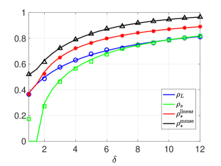
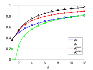
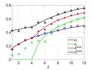
We highlight that, even if one of the two estimators is ineffective, the proposed optimal combination can still improve on the performance of the other one. This is due to the fact that the function takes advantage of the knowledge of the signal prior. We showcase an example of this behavior for a binary prior in Figure 5 discussed in Section 4.2. We also note that if the signal prior is Gaussian, then no improvement is possible when one of the two estimators has vanishing correlation with the signal, see Figures 2-4 in Section 4.1. In fact, as detailed in Section 3.3, in the Gaussian case is a linear combination of and . Thus, if (resp. ), then is aligned with (resp. ).
Remark 3.4 (Sign of ).
The spectral estimator is defined up to a change of sign, since it is the principal eigenvector of a suitable matrix. In Theorem 1 and 2, we pick the sign of such that . In practice, there is a simple way to resolve the sign ambiguity: one can match the sign of as defined in (3.3) with the sign of the scalar product (see also (3.19)).
Remark 3.5 (Sufficient condition for pseudo-Lipschitz ).
The assumption that the Bayes-optimal estimator in (3.7) is pseudo-Lipschitz is fairly mild. In fact, is Lipschitz if either of the following two conditions on hold [FVRS21, Lemma 3.8]: (i) has a log-concave distribution, or (ii) there exist independent random variables such that is Gaussian, is compactly supported and .
Remark 3.6 (Non-separable combinations).
The optimality of in Theorem 2 can be extended to a class of combined estimators of the form , where may not act component-wise on . Given , we define the function . Let be any sequence of functions (indexed by ) such that is uniformly pseudo-Lipschitz of order . That is, for each , the property (3.4) holds for with a pseudo-Lipschitz constant that does not depend on . Then, the state evolution result in [BMN20, Theorem 1] for non-separable test functions implies that
| (3.15) |
The result above is in terms of convergence in probability, while the limiting statement in (3.13) holds almost surely. This is because the state evolution result for AMP with non-separable functions [BMN20, Theorem 1] is obtained in terms of convergence in probability.
3.3 A Special Case: Optimal Linear Combination
Theorem 2 shows that the optimal way to combine and is via the Bayes-optimal estimator for the corresponding scalar problem. If the signal prior is standard Gaussian, then is a linear combination of and . In this section, we provide closed-form expressions for the performance of such optimal linear combination.
For convenience, let us denote the normalized linear estimator as , i.e., . (Recall that the spectral estimator is already normalized, i.e., .) We consider an estimator of , parameterized by , defined as follows:
| (3.16) |
where we use the convention, for .
Let us now compute the asymptotic performance of the proposed estimator in (3.16). Specifically, using Lemmas 2.1 and 2.2, it follows immediately that
| (3.17) |
In order to conclude with the limit of the normalized correlation , it still remains to compute the magnitude of the new estimator:
| (3.18) |
This is possible thanks to the following result, which gives the correlation between the linear and the spectral estimator as well as the asymptotic performance of the linear combination .
Corollary 3.3 (Performance of linear combination).
Proof.
Using (3.1), the parameter can be alternatively expressed in terms of and in the following compact form:
| (3.21) |
Observe also that and .
Using the characterization of Corollary 3.3, we can compute the combination coefficient that leads to the asymptotically optimal linear combination of the form (3.16).
Corollary 3.4 (Optimal linear combination).
Recall the notation in Corollary 3.3 and define
| (3.22) |
Assume . Then, for all , it holds that
| (3.23) |
The proof of Corollary 3.3 is deferred to Appendix B. Let us now comment on the assumption . If and are perfectly correlated (i.e., ), then it is clear that the combined estimator cannot improve the performance for any value of . On the contrary, when , Corollary 3.4 characterizes when the linear combination strictly improves upon the performance of the individual estimators and . Specifically, by denoting
| (3.24) |
such that the right-hand side of (3.23) becomes
| (3.25) |
it can be readily checked that provided that and .
Remark 3.7 (Optimization of preprocessing functions).
The linear estimator and the spectral estimator use the preprocessing functions (cf. (1.3)) and (cf. (1.4)), respectively. The choice of these functions naturally affects the performance of the two estimators, as well as, that of the combined estimator . Lemmas 2.1-2.2, Theorem 2 and Corollary 3.4 derive sharp asymptotics on the estimation performance that hold for any choice of the preprocessing functions and satisfying our technical assumptions (A1), (A2), (A3), (B2). In Appendix C, we briefly discuss how these results can be used to yield optimal such choices. Specifically, the optimal preprocessing function that maximizes the normalized correlation of the spectral estimator is derived in [LAL19], see Appendix C.2. The optimal choice for the linear estimator is much easier to obtain and we outline the process in Appendix C.1. In Appendix C.3, we combine these two results to derive a precise characterization of the sampling regimes in which the linear estimator surpasses the spectral estimator, and vice-versa. Finally, in Appendix C.4, we use Corollary 3.4 to cast the problem of optimally choosing and to maximize the correlation of the combined estimator as a function optimization problem. Solving the latter is beyond the scope of this paper, and it represents an intriguing future research direction.
4 Numerical Simulations
This section validates our theory via numerical experiments and provides further insights on the benefits of the proposed combined estimator.
First, we consider a setting in which the signal is uniformly distributed on the -dimensional sphere. In this case, the limiting empirical distribution is Gaussian. Thus, the Bayes-optimal estimator in (3.7) is linear and is given by , where is determined in Corollary 3.4. For this scenario, we study in Figures 2, 3 and 4 the performance gain of for three different measurement models and for various noise levels.
Second, in Figure 5 we consider a setting in which the the entries of are binary, drawn i.i.d. from the set , such that the empirical distribution is of the form , for some . For this case, we compute the Bayes-optimal estimator and compare it with the optimal linear combination for various choices of output functions.
4.1 Optimal Linear Combination
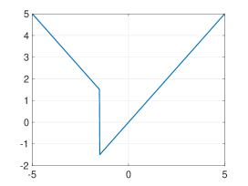
In Figure 2, we fix the input-output relation as , with and (cf. Figure 2(a)), and we investigate the performance gain of the proposed combined estimator for different values of the noise variance . Here, is generated via a standard Gaussian vector which is normalized such that . Also, and the pre-processing functions are chosen: and . Note that the empirical distribution of tends to a standard Gaussian distribution in the high-dimensional limit. Thus, following Section 3.3, the optimal combined estimator is (asymptotically) linear and is given by (3.16) for chosen as in (3.22). In Figure 2(b), we plot the percentage improvement as a function of the sampling ratio , for three values of the noise variance and . Here, defined in (3.23) and We observe that, as increases, larger values of the sampling ratio are needed for the combined estimator to improve upon the linear and spectral estimators. However, for sufficiently large , the benefit of the combined estimator is more pronounced for larger values of the noise variance. For instance, for and large values of , the percentage gain is larger than . In Figure 2(c), we fix and plot the correlations and . The solid lines correspond to the theoretical predictions obtained by Lemma 2.1, Lemma 2.2 and Corollary 3.4, respectively. The theoretical predictions are compared against the results of Monte Carlo simulations. For the simulations, we used and averaged over independent problem realizations. In Figure 2(c)(Middle), we also plot the limit (cf. (3.3)) of the cross-correlation and the ratio in (3.24). The corresponding values of the optimal combination coefficient are plotted in Figure 2(c)(Right). For values of smaller than the threshold for weak-recovery of the spectral method (where ), we observe that and . However, for larger values of , the value of the optimal coefficient is non trivial. Finally, Figure 2(d) shows the same plots as in Figure 2(c), but for .
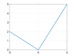
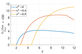


The setting of Figure 3 is the same as in Figure 2, only now the input-output function is chosen as . Comparing Figure 3(b) to Figure 2(b), note that the benefit of the combined estimator is more significant for the link function studied here. Moreover, in contrast to Figure 2(b), here, the percentage gain of the combined estimator takes its maximum value in the noiseless case: .
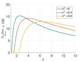


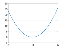
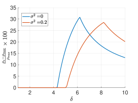


In Figure 4, we repeat the experiments of Figures 2 and 3, but for . Compared to the two functions studied in Figures 2 and 3, in Figure 4 we observe that the performance gain is significantly larger and reaches values up to . This can be argued by considering the expansion of the input-output functions on the basis of the Hermite polynomials, i.e., , where is the th-order Hermite polynomial with leading coefficient and . Specifically, recall that the first three Hermite polynomials are as follows: , and . Thus, for , only the first three coefficients , are non-zero. To see the relevance of these coefficients to the linear and spectral estimators note that for identity pre-processing functions it holds that and Thus, it follows directly from Lemma 2.1 that if the first Hermite coefficient is zero. Similarly, it can be shown using Lemma 2.2 that if the second Hermite coefficient is zero; in fact, the threshold of weak recovery of the spectral method is infinity in this case (see (C.7) in Appendix C). Intuitively, the linear and spectral estimators exploit the energy of the output function corresponding to the Hermite polynomials of first- and second-order, respectively; see also [DH18, TR19]. In this example, we have chosen such that all of its energy is concentrated on the Hermite polynomials of order up to two.
As a final note, from the numerical results in Figures 2, 3 and 4, we observe that the proposed optimal combination leads to a performance improvement only if both the linear and the spectral estimators are asymptotically correlated with the signal. This is because the signal prior is Gaussian (see Remark 3.3). In contrast, as we will see in the next section, when the signal prior is binary, the combined estimator provides an improvement even when only the linear estimator is effective.
4.2 Bayes-optimal Combination
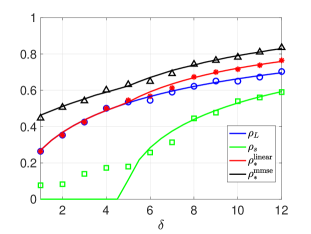
In Figures 5(a,b) and 5(c,d) we consider the same setting as in Figures 3 and 4, respectively. However, here each entry of takes value either or . Each entry is chosen independently according to the distribution , for . Thus, the Bayes optimal combination is not necessarily linear as in the Gaussian case. In Appendix D, we compute the Bayes-optimal estimator (cf. (3.7)) for the setting considered here. Then, we use the prediction of Theorem 2 to plot in solid black lines the normalized correlation of with (i.e., in (3.12)). The theoretical predictions (solid lines) are compared against the results of Monte Carlo simulations (markers). Moreover, we compare the optimal performance against those of the linear estimator (cf. ), the spectral estimator (cf. ) and the optimal linear combination (cf. . We have chosen in Figures 5(a,c) and in Figures 5(b,d). Note that the optimal linear combination provides a performance improvement only for the values of s.t. and . On the contrary, is strictly larger than even when .
4.3 The Combined Estimator as Initialization for Local Algorithms
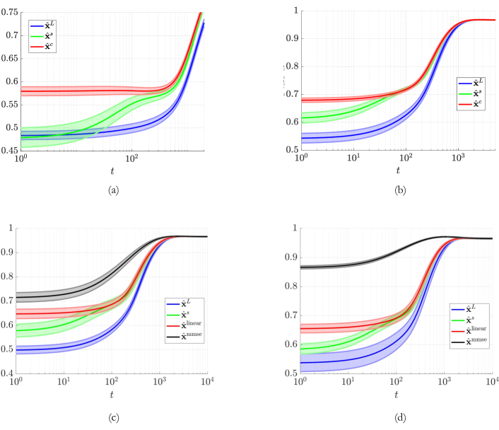
As mentioned in the introduction, the initial estimates of the signal obtained by either the linear/spectral methods or our proposed combined estimator, can then be refined via local algorithms such as gradient descent (GD). The theory and numerical simulations in the previous sections showed the superiority of our proposed combined estimator over and in terms of correlation with the true signal. In Figure 6, by plotting the correlation of GD iterates for different initializations, we show numerically how this improvement translates to improved performance of gradient descent refinements. Specifically, we ran GD on squared error loss with step size , that is . Here, is the output function described in the caption of the figure.
In Figures 6(a,b), the true signal has i.i.d. Gaussian entries, thus the linear combined estimator is the optimal combination in terms of correlation performance. We observe that for two different choices of output function and sampling ratio (see caption), GD with linear or spectral initialization requires hundreds of iterations to reach the performance of the combined estimator. In Figures 6(c,d), the true signal has entries in , chosen independently with and , respectively. Here, the linear combined estimator is sub-optimal (but still improves upon linear/spectral), thus we also compute and study the Bayes-optimal estimator. Interestingly, while for both priors, GD converges to the same correlation as increases, for , GD achieves higher correlation if stopped early. It is a fascinating, albeit challenging, question to better understand the evolution of the GD trajectory as a function of the initialization, signal prior and output function.
5 Proof of Theorem 1
5.1 Proof Sketch
The proof of Theorem 1 is based on the design and analysis of a generalized approximate message passing (GAMP) algorithm. GAMP is a class of iterative algorithms proposed by Rangan [Ran11] for estimation in generalized linear models. A GAMP algorithm is defined in terms of a sequence of Lipschitz functions and , for . For , the GAMP iteration computes:
| (5.1) |
Here, the functions and are understood to be applied component-wise, i.e., , and . The scalars are defined as
| (5.2) |
where denotes the derivative with respect to the first argument. The iteration (5.1) is initialized with
| (5.3) |
for some constant . Here, denotes the all-ones vector.
A key feature of the GAMP algorithm (5.1) is that the asymptotic empirical distribution of its iterates can be succinctly characterized via a deterministic recursion, called state evolution. Hence, the performance of the high-dimensional problem involving the iterates is captured by a scalar recursion. Specifically, this result gives that for , the empirical distributions of and converge in distance to the laws of the random variables and , respectively, with
| (5.4) | ||||
| (5.5) |
where . Similarly, and are independent. The deterministic parameters , are computed via the recursion (5.9) detailed in Section 5.2, and the formal statement of the state evolution result is contained in Proposition 5.1 (again in Section 5.2).
Next, in Section 5.3, we show that a suitable choice of the functions leads to a GAMP algorithm such that (i) , and (ii) is aligned with as grows large. Specifically, choosing in (5.3) immediately gives . In order to approach the spectral estimator as , we pick to be linear functions; see (5.21). The idea is that, with this choice of and , the GAMP iteration is effectively a power method. Let us now briefly discuss why this is the case. With the choice of in (5.21), the GAMP iteration can be expressed as
| (5.6) |
where , , and the function is defined later in terms of the spectral preprocessing function ; see (5.35). Then, Lemma 5.2 analyzes the fixed points of the state evolution of the GAMP algorithm (5.6), and Lemma 5.34 proves that in the high-dimensional limit, the vector tends to align with the principal eigenvector of the matrix as . Here, we provide a heuristic sanity check for this last claim. Assume that the iterates and converge to the limits and , respectively, in the sense that and . Then, from (5.6), the limits and satisfy
| (5.7) |
Furthermore, from the analysis of the fixed points of state evolution of Lemma 5.2, we obtain that . Thus, after some manipulations, (5.7) can be rewritten as
| (5.8) |
Hence, is an eigenvector of the matrix , and the GAMP algorithm is effectively performing a power method. Finally, we choose (and consequently ) so that , with given by (2.8). In this way, the matrix coincides with the spectral matrix , as defined in (2.9), and therefore approaches the spectral estimator .
In conclusion, as and tends to be aligned with for large , we can use the state evolution result of Proposition 5.1 to analyze the joint empirical distribution of . At this point, the proof of Theorem 1 becomes a straightforward application of Lemma 5.34, and is presented at the end of Section 5.3. The proof of Lemma 5.34 is quite long, so it is provided separately in Section 5.4.
5.2 State Evolution for Generalized Approximate Message Passing (GAMP)
For , let us define the following deterministic recursion for the parameters , appearing in (5.4)-(5.5):
| (5.9) |
Recalling from (5.3) that , the state evolution recursion is initialized with
| (5.10) |
Furthermore, for , let the sequences of random variables and be each jointly Gaussian with zero mean and covariance defined as follows [RV18, BMN20]. First, we have:
| (5.11) |
Then, for , we iteratively compute:
| (5.12) | ||||
| (5.13) |
Note that for , by (5.9) we have .
At this point, we are ready to present the state evolution result [Ran11, JM13] for the GAMP algorithm (5.1)-(5.2).
5.3 GAMP as a Power Method to Compute the Spectral Estimator
Consider the GAMP iteration in (5.1) initialized with , and the function chosen as
| (5.19) |
so that
| (5.20) |
(The function is assumed to be zero.) From (2.6), we note that .
For , let the functions and be chosen as
| (5.21) |
where the function is bounded and Lipschitz, and is a constant, defined iteratively for via the state evolution equations below (Eqs. (5.25)-(5.27)). To prove Theorem 1, we will choose as a suitable function of (see (5.35)). Note that the functions and are required to be Lipschitz for , and this will be ensured choosing to be bounded and Lipschitz (see Lemma 5.34 below).
With this choice of , for , the scalars in (5.2) are given by
| (5.22) |
In the GAMP iteration below, we will replace the parameter by its almost sure limit , where . The state evolution result in Proposition 5.1 still holds when is replaced with in the GAMP iteration [Ran11, JM13]. This can be shown using the pseudo-Lipschitz property of the test functions in Eqs. (5.14)-(5.15) and the fact that almost surely, due to the strong law of large numbers.
With these choices, the GAMP iteration in (5.1) is as follows. Initializing with
| (5.23) |
we have for :
| (5.24) |
where and . The state evolution equations in (5.9) become:
| (5.25) | |||
| (5.26) | |||
| (5.27) |
Here, we recall that and , for . From (5.10), the state evolution iteration is initialized with the following:
| (5.28) |
We will show in Lemma 5.34 that in the high-dimensional limit, the vector in (5.24) tends to align with the principal eigenvector of the matrix as . In other words, the GAMP iteration is equivalent to a power iteration for . This equivalence, together with Proposition 5.1, allows us to precisely characterize the limiting empirical distribution of the eigenvector of in Lemma 5.34.
We begin with a result characterizing the fixed points of the state evolution recursion in (5.25)-(5.26).
Lemma 5.2.
Assume that and that . Then, the state evolution recursion (5.25)-(5.26) has three fixed points: one is , and the other two are and , where
| (5.29) |
with
| (5.30) |
Furthermore, if the initialization (5.28) is such that , then the recursion converges to . If , the recursion converges to .
The lemma is proved in Appendix E. We note that Lemma 5.2 (and the subsequent Lemmas 5.3-5.34 as well) assumes that and . These conditions concern the auxiliary random variable (or, equivalently, the auxiliary function ). In the proof of Theorem 1, which appears at the end of this section, we will provide a choice of (depending on ) that fulfills these requirements; see (5.35). Let us also point out that the condition follows from , which in turn ensures that . For a discussion of the case , see Remark 3.1.
The next lemma shows that the mean-squared difference between successive AMP iterates vanishes as in the high-dimensional limit.
Lemma 5.3.
Assume that , , and . Consider the GAMP iteration in (5.24) initialized with . Then, the following limits hold almost surely:
| (5.31) |
The proof of the lemma is given in Appendix F. The next result is the main technical lemma needed to prove Theorem 1. It shows that, as grows large, tends to be aligned with the principal eigenvector of the matrix defined in (5.32) below. Theorem 1 is then obtained from Lemma 5.34 by using a suitable choice for in the GAMP iteration (5.24), which ensures that is a scaled version of in (2.9).
Lemma 5.4.
Let be such that , , and be distributed according to (2.3). Let , and for . Assume that the conditions (B1)-(B2) on p.3 hold (with replaced by in (B2)). Assume also that is bounded, , and . Define and assume that satisfies the assumptions (A1), (A2), (A3) on p. 2.4. Define the matrix
| (5.32) |
where . Let be the principal eigenvector of , let its sign be chosen so that , and consider the rescaling . Also, let , where is the linear estimator defined in (2.6).
We first show how Theorem 1 is obtained from Lemma 5.34, and then prove the lemma in the following subsection.
Proof of Theorem 1.
Recall that is the unique solution of (2.16) for , where is the supremum of the support of . Define
| (5.35) |
We now verify that satisfies the assumptions of Lemma 5.34. As and has bounded support with supremum , we have that is bounded. Furthermore, is a Lipschitz function of , since is a Lipschitz function of and is bounded away from . Thus, satisfies the condition (B2) (with replaced by ).
Next, note that (since satisfies assumption (A3)). As , we have that .
As , we have that , where denotes the point at which attains its minimum (see Eq. (2.14)). Consequently, since solves (2.16), we have that
| (5.36) |
As satisfies assumption (A3), we have that , which implies that . Thus, by using the definitions (2.12)-(2.13), (5.36) can be rewritten as
| (5.37) |
By combining (5.35) and (5.37), we obtain that
| (5.38) |
Finally, we compute the derivative of at , noting that the derivative and the expectation in (2.13) can be interchanged due to bounded convergence. We thus obtain that the condition is equivalent to
| (5.39) |
where the last equality follows from (5.35). From (5.38) and (5.39), we have .
5.4 Proof of Lemma 5.34
Fix , and let and . Then,
| (5.41) |
Thus, by inspecting the definition (5.32), one immediately obtains that does not change if we rescale and by the multiplicative factor . Furthermore, by using the definitions (5.29)-(5.30), we have that
| (5.42) |
| (5.43) |
and that
| (5.44) |
Consequently, both the LHS and the RHS of (5.33) are unchanged when we rescale and by the multiplicative factor .
The argument above proves that, without loss of generality, we can rescale and by any multiplicative factor . To simplify the rest of the argument, it is convenient to assume the normalization condition
| (5.45) |
under which .
Consider the iteration (5.24) with the initialization in (5.23). Since by hypothesis, , Lemma 5.2 guarantees that the state evolution recursion (5.26) converges to either fixed point or as . That is,
| (5.46) |
The last equality above follows by combining (5.30) and (5.45).
By substituting the expression for in (5.24) in the update, the iteration can be rewritten as follows, for :
| (5.47) | ||||
| (5.48) |
In the remainder of the proof, we will assume that . Define
| (5.49) | ||||
| (5.50) |
By combining (5.49) with (5.47), we have that
| (5.51) |
By substituting the expression for obtained in (5.51) into (5.48), we have
| (5.52) |
Let
| (5.53) |
From (5.50) and (5.52), we obtain
| (5.54) |
Let us decompose into a component in the direction of plus an orthogonal component :
| (5.55) |
where .
At this point, the idea is to show that, when is large, is small, thus tends to be aligned with . To do so, we prove that, as , the largest eigenvalue of the matrix defined in (5.32) converges almost surely to . Furthermore, we prove that the matrix exhibits a spectral gap, in the sense that the second largest eigenvalue of converges almost surely to a value strictly smaller than . Since is orthogonal to and has a spectral gap, the norm of in (5.53) can be lower bounded by a strictly positive constant times the norm of . Next, using the expression in (5.54), we show that the norm of can be made arbitrarily small by taking and sufficiently large. From this, we conclude that must be small.
We begin by proving that has a spectral gap.
Lemma 5.5 (Spectral gap for ).
The following holds almost surely:
| (5.56) | ||||
| (5.57) |
for a numerical constant that does not depend on .
Proof of Lemma 5.5.
By hypothesis, satisfies the assumptions (A1)-(A2)-(A3). Thus, we can use Lemma 2.2 to compute the almost sure limit of the two largest eigenvalues of , call them .
Let denote the supremum of the support of . As and has bounded support, we have that . For , define
| (5.58) |
and
| (5.59) |
Note that
| (5.60) |
Thus, by using (5.45), we have that
| (5.61) |
Furthermore,
| (5.62) |
Thus,
| (5.63) |
where in the last step we combine the hypothesis with the normalization condition (5.45).
Let be the point at which attains its minimum, as defined in (2.14), define as in (2.15) and let be the unique solution of (2.16). Since is convex, (5.62) and (5.63) imply that . Furthermore, (5.61) implies that . By Lemma 2.2, we obtain that, as ,
| (5.64) |
Note that
| (5.65) |
where the first equality comes from the fact that is the unique solution of (2.16), while the second and third equalities follow from (5.60) and (5.61). By combining (5.65) and (5.64), we obtain . Furthermore, . As and is Lipschitz continuous (from (5.62)), there exists a numerical constant such that
| (5.66) |
Hence, . ∎
Let us now go back to (5.53) and combine it with (5.55). Then,
| (5.67) |
We now prove that, almost surely, for all sufficiently large , the following lower bound on the norm of the LHS of (5.67) holds:
| (5.68) |
where is a numerical constant independent of .
As the matrix is symmetric, it can be written in the form , with orthogonal and diagonal. Furthermore, the columns of are the eigenvectors of and the diagonal entries of are the corresponding eigenvalues. As is orthogonal to , we can write
| (5.69) |
where is obtained from by changing the entry corresponding to to any other value. For our purposes, it suffices to substitute with . Note that
| (5.70) |
where denotes the smallest eigenvalue of and the last equality follows from the variational characterization of the smallest eigenvalue of a symmetric matrix. Note that
| (5.71) |
By using (5.57), we obtain that, almost surely, for all sufficiently large ,
| (5.72) |
By combining (5.69), (5.70), (5.71) and (5.72), we conclude that (5.68) holds.
Recalling that satisfies (5.67), we will next show that, almost surely,
| (5.73) |
Combined with (5.67) and (5.68), this implies that almost surely.
By using the triangle inequality, we have
| (5.74) |
where the second inequality uses and that .
We can bound the second term on the RHS of (5.74) using the result in Proposition 5.1, applied with the PL(2) test function . Then, almost surely,
| (5.75) |
Here we used the definitions of and from (5.5) and (5.27). Recalling from (5.46) that , the limit in (5.75) combined with Remark 5.1 and the continuous mapping theorem implies that, almost surely,
| (5.76) |
Thus, by using (5.56), we conclude that, almost surely,
| (5.77) |
We now bound the first term on the RHS of (5.74). Recalling the definition of in (5.54), an application of the triangle inequality gives
| (5.78) |
where the second inequality follows from the fact that, given a matrix and a vector , .
Let us bound the operator norm of the two matrices appearing in the RHS of (5.78). As the operator norm is sub-multiplicative, we have
| (5.79) |
As is bounded, the operator norm of is upper bounded by a numerical constant (independent of ). The operator norm of and is also upper bounded by a numerical constant (independent of ). Indeed, from (5.46) as , and the support of does not contain points arbitrarily close to . We also have that, almost surely, for all sufficiently large , the operator norm of is upper bounded by a constant (independent of ). As a result, we deduce that, almost surely, for all sufficiently large ,
| (5.80) |
where is a numerical constant (independent of ). Furthermore, by Lemma 5.3, the following limits hold almost surely:
| (5.81) |
By combining (5.46), (5.76), (5.80) and (5.81), we obtain that, almost surely, each of the terms in the RHS of (5.78) vanishes when scaled by the factor , as . As a result, almost surely,
| (5.82) |
By combining (5.74), (5.77) and (5.82), we conclude that, almost surely, (5.73) holds.
Recall that satisfies (5.67). Thus, by combining the lower bound in (5.68) with the almost sure limit in (5.73), we obtain that, almost surely,
| (5.83) |
Recalling from (5.55) that is the component of orthogonal to , the result in (5.83) implies that tends to be aligned with in the high-dimensional limit. In formulas, by combining (5.55) with (5.83), we have that, almost surely,
| (5.84) |
Note that
| (5.85) |
Thus, by using (5.76), we obtain that, almost surely,
| (5.86) |
To obtain the sign of , we first observe that, by Proposition 5.1, almost surely,
| (5.87) |
As and , the state evolution iteration (5.26) implies that for all . Using (5.55) we can write
| (5.88) |
Recall that by hypothesis, . Moreover, using (5.83) and Cauchy-Schwarz, we have almost surely. Thus we deduce that almost surely. Therefore,
| (5.89) |
with .
At this point, we are ready to prove (5.33). For any function , we have that
| (5.90) |
where are universal constants (which may depend on but not on ). The inequality in the second line above uses , and the third and fourth lines are obtained via the Hölder and Cauchy-Schwarz inequalities. We now claim that, almost surely,
| (5.91) |
where, from now on, we will use to denote a generic positive constant that does not depend on . If (5.91) holds, then by using (5.89) and (5.90), we deduce that, almost surely,
| (5.92) |
Let us now prove (5.91). First, by assumption (B1), we have that
| (5.93) |
Next, the main technical lemma [JM13, Lemma 2] leading to the state evolution result in Proposition 5.1 implies that, almost surely, for ,
| (5.94) |
In particular, this follows from [JM13, Lemma 2(e)] (see also [BM11, Lemma 1(e)]). Since , we also have that, almost surely,
| (5.95) |
It remains to show that, almost surely,
| (5.96) |
To do so, we use a rotational invariance argument. Let be an orthogonal matrix such that . Then,
| (5.97) |
Consequently, we have that
| (5.98) |
which immediately implies that
| (5.99) |
Then, we can decompose as
| (5.100) |
where is uniformly distributed over the set of vectors orthogonal to with norm and
| (5.101) |
Relating the uniform distribution on the sphere to the normal distribution [Ver18, Sec. 3.3.3], we can express as follows:
| (5.102) |
where and independent of . By the law of large numbers, we have the almost sure limits
| (5.103) |
Thus, by combining (5.100) and (5.102), we conclude that
| (5.104) |
where the coefficients and can be bounded by universal constants (independent of ) using (5.103). As a result,
| (5.105) |
Note that, almost surely,
| (5.106) |
where . By combining (5.93), (5.105) and (5.106), (5.96) immediately follows. Finally, by combining (5.93), (5.94), (5.95) and (5.96), we deduce that (5.91) holds.
We now use Proposition 5.1 which guarantees that, almost surely,
| (5.107) |
To conclude the proof of (5.33), we take the limit and use Remark 5.1. For this, we will show that
| (5.108) |
where are zero mean jointly Gaussian random variables with covariance given by (5.34). Using (5.11) and the formulas for and from (5.19) and (5.21), we have
| (5.109) |
In the second equality above, we used (5.25). Using the expression for from (5.28) and letting , we have
| (5.110) |
Therefore, the sequence of zero mean jointly Gaussian pairs converges in distribution to the jointly Gaussian pair , whose covariance is given by (5.34).
To show (5.108), we use Lemma G.1 in Appendix G. We apply this result taking to be the distribution of
Since , , the sequence converges weakly to , which is the distribution of
In our case, is PL(), and therefore , for all for some constant . Choosing , we have . Furthermore, is a linear combination of , with coefficients that do not depend on . The integral has the same form, except that are replaced by , respectively. Since and , we have that
Therefore, by applying Lemma G.1 in Appendix G, we have that
which is equivalent to (5.108). This completes the proof of the lemma.
Acknowledgements
M. Mondelli would like to thank Andrea Montanari for helpful discussions. M. Mondelli was partially supported by the 2019 Lopez-Loreta Prize. C. Thrampoulidis was partially supported by an NSF award CIF-2009030. R. Venkataramanan was partially supported by the Alan Turing Institute under the EPSRC grant EP/N510129/1.
References
- [BB08] Petros T Boufounos and Richard G Baraniuk, 1-bit compressive sensing, 42nd Annual Conference on Information Sciences and Systems, IEEE, 2008, pp. 16–21.
- [BBAP05] Jinho Baik, Gérard Ben Arous, and Sandrine Péché, Phase transition of the largest eigenvalue for nonnull complex sample covariance matrices, Annals of Probability (2005), 1643–1697.
- [BKM+19] Jean Barbier, Florent Krzakala, Nicolas Macris, Léo Miolane, and Lenka Zdeborová, Optimal errors and phase transitions in high-dimensional generalized linear models, Proceedings of the National Academy of Sciences 116 (2019), no. 12, 5451–5460.
- [BM11] Mohsen Bayati and Andrea Montanari, The dynamics of message passing on dense graphs, with applications to compressed sensing, IEEE Transactions on Information Theory 57 (2011), 764–785.
- [BM12] M. Bayati and A. Montanari, The LASSO risk for gaussian matrices, IEEE Transactions on Information Theory 58 (2012), 1997–2017.
- [BMN20] Raphael Berthier, Andrea Montanari, and Phan-Minh Nguyen, State evolution for approximate message passing with non-separable functions, Information and Inference 9 (2020), no. 1, 33–79.
- [BR17] Sohail Bahmani and Justin Romberg, Phase retrieval meets statistical learning theory: A flexible convex relaxation, International Conference on Artificial Intelligence and Statistics (AISTATS), 2017, pp. 252–260.
- [Bri82] David R Brillinger, A generalized linear model with Gaussian regressor variables, A Festschrift For Erich L. Lehmann (1982), 97.
- [CC15] Yuxin Chen and Emmanuel J. Candès, Solving random quadratic systems of equations is nearly as easy as solving linear systems, Advances in Neural Information Processing Systems (NIPS), 2015, pp. 739–747.
- [CESV15] Emmanuel J. Candès, Yonina C. Eldar, Thomas Strohmer, and Vladislav Voroninski, Phase retrieval via matrix completion, SIAM Review 57 (2015), no. 2, 225–251.
- [CLS15] Emmanuel J. Candès, Xiaodong Li, and Mahdi Soltanolkotabi, Phase retrieval via Wirtinger flow: Theory and algorithms, IEEE Transactions on Information Theory 61 (2015), no. 4, 1985–2007.
- [CSV13] Emmanuel J. Candès, Thomas Strohmer, and Vladislav Voroninski, Phaselift: Exact and stable signal recovery from magnitude measurements via convex programming, Communications on Pure and Applied Mathematics 66 (2013), no. 8, 1241–1274.
- [DBMM20] Rishabh Dudeja, Milad Bakhshizadeh, Junjie Ma, and Arian Maleki, Analysis of spectral methods for phase retrieval with random orthogonal matrices, IEEE Transactions on Information Theory 66 (2020), no. 8, 5182–5203.
- [DH18] Rishabh Dudeja and Daniel Hsu, Learning single-index models in Gaussian space, Conference On Learning Theory (COLT), 2018, pp. 1887–1930.
- [DM14] Yash Deshpande and Andrea Montanari, Information-theoretically optimal sparse PCA, IEEE International Symposium on Information Theory (ISIT), 2014, pp. 2197–2201.
- [DMM09] David L. Donoho, Arian Maleki, and Andrea Montanari, Message Passing Algorithms for Compressed Sensing, Proceedings of the National Academy of Sciences 106 (2009), 18914–18919.
- [DSS11] Lutz Dümbgen, Richard Samworth, and Dominic Schuhmacher, Approximation by log-concave distributions, with applications to regression, Annals of Statistics 39 (2011), no. 2, 702–730.
- [DTL18] Oussama Dhifallah, Christos Thrampoulidis, and Yue M Lu, Phase retrieval via polytope optimization: Geometry, phase transitions, and new algorithms, arXiv:1805.09555 (2018).
- [EK12] Yonina C Eldar and Gitta Kutyniok, Compressed sensing: Theory and applications, Cambridge University Press, 2012.
- [Fie82] J. R. Fienup, Phase retrieval algorithms: A comparison, Applied Optics 21 (1982), no. 15, 2758–2769.
- [FVRS21] Oliver Y. Feng, Ramji Venkataramanan, Cynthia Rush, and Richard J. Samworth, A unifying tutorial on approximate message passing, arXiv:2105.02180 (2021).
- [Gen17] Martin Genzel, High-dimensional estimation of structured signals from non-linear observations with general convex loss functions, IEEE Transactions on Information Theory 63 (2017), no. 3, 1601–1619.
- [GJ19] Martin Genzel and Peter Jung, Recovering structured data from superimposed non-linear measurements, IEEE Transactions on Information Theory 66 (2019), no. 1, 453–477.
- [GMW18] Larry Goldstein, Stanislav Minsker, and Xiaohan Wei, Structured signal recovery from non-linear and heavy-tailed measurements, IEEE Transactions on Information Theory 64 (2018), no. 8, 5513–5530.
- [GS18] Tom Goldstein and Christoph Studer, Phasemax: Convex phase retrieval via basis pursuit, IEEE Transactions on Information Theory 64 (2018), no. 4, 2675–2689.
- [HR04] David C Hoyle and Magnus Rattray, Principal-component-analysis eigenvalue spectra from data with symmetry-breaking structure, Physical Review E 69 (2004), no. 2, 026124.
- [JM13] Adel Javanmard and Andrea Montanari, State evolution for general approximate message passing algorithms, with applications to spatial coupling, Information and Inference (2013), 115–144.
- [KKSK11] Sham M Kakade, Varun Kanade, Ohad Shamir, and Adam Kalai, Efficient learning of generalized linear and single index models with isotonic regression, Advances in Neural Information Processing Systems (NIPS), 2011, pp. 927–935.
- [KMS+12] Florent Krzakala, Marc Mézard, Francois Sausset, Yifan Sun, and Lenka Zdeborová, Probabilistic reconstruction in compressed sensing: algorithms, phase diagrams, and threshold achieving matrices, Journal of Statistical Mechanics: Theory and Experiment 2012 (2012), no. 08, P08009.
- [LAL19] Wangyu Luo, Wael Alghamdi, and Yue M. Lu, Optimal spectral initialization for signal recovery with applications to phase retrieval, IEEE Transactions on Signal Processing 67 (2019), no. 9, 2347–2356.
- [LBH15] Yann LeCun, Yoshua Bengio, and Geoffrey Hinton, Deep learning, Nature 521 (2015), no. 7553, 436–444.
- [LD89] Ker-Chau Li and Naihua Duan, Regression analysis under link violation, Annals of Statistics (1989), 1009–1052.
- [Li92] Ker-Chau Li, On principal Hessian directions for data visualization and dimension reduction: Another application of Stein’s lemma, Journal of the American Statistical Association 87 (1992), no. 420, 1025–1039.
- [LKZ17] Thibault Lesieur, Florent Krzakala, and Lenka Zdeborová, Constrained low-rank matrix estimation: Phase transitions, approximate message passing and applications, Journal of Statistical Mechanics: Theory and Experiment 2017 (2017), no. 7, 073403.
- [LL19] Yue M. Lu and Gen Li, Phase transitions of spectral initialization for high-dimensional non-convex estimation, Information and Inference (2019).
- [McC18] Peter McCullagh, Generalized linear models, Routledge, 2018.
- [MM19] Marco Mondelli and Andrea Montanari, Fundamental limits of weak recovery with applications to phase retrieval, Foundations of Computational Mathematics 19 (2019), 703–773.
- [MV21] Andrea Montanari and Ramji Venkataramanan, Estimation of low-rank matrices via approximate message passing, Annals of Statistics 45 (2021), no. 1, 321–345.
- [NJS13] Praneeth Netrapalli, Prateek Jain, and Sujay Sanghavi, Phase retrieval using alternating minimization, Advances in Neural Information Processing Systems (NIPS), 2013, pp. 2796–2804.
- [NLC16] Matey Neykov, Jun S Liu, and Tianxi Cai, L1-regularized least squares for support recovery of high dimensional single index models with gaussian designs, The Journal of Machine Learning Research 17 (2016), no. 1, 2976–3012.
- [NW72] John Ashworth Nelder and Robert WM Wedderburn, Generalized linear models, Journal of the Royal Statistical Society: Series A (General) 135 (1972), no. 3, 370–384.
- [PV16] Yaniv Plan and Roman Vershynin, The generalized lasso with non-linear observations, IEEE Transactions on Information Theory 62 (2016), no. 3, 1528–1537.
- [PVY17] Yaniv Plan, Roman Vershynin, and Elena Yudovina, High-dimensional estimation with geometric constraints, Information and Inference 6 (2017), no. 1, 1–40.
- [Ran11] S. Rangan, Generalized Approximate Message Passing for Estimation with Random Linear Mixing, IEEE International Symposium on Information Theory (ISIT), 2011.
- [RFG09] S. Rangan, A. K. Fletcher, and V. K. Goyal, Asymptotic Analysis of MAP Estimation via the Replica Method and Applications to Compressed Sensing, Advances in Neural Information Processing Systems (NIPS), 2009.
- [RG01] Sundeep Rangan and Vivek K. Goyal, Recursive consistent estimation with bounded noise, IEEE Transactions on Information Theory 47 (2001), no. 1, 457–464.
- [RV18] Cynthia Rush and Ramji Venkataramanan, Finite sample analysis of approximate message passing algorithms, IEEE Transactions on Information Theory 64 (2018), no. 11, 7264–7286.
- [SC19] Pragya Sur and Emmanuel J Candès, A modern maximum-likelihood theory for high-dimensional logistic regression, Proceedings of the National Academy of Sciences 116 (2019), no. 29, 14516–14525.
- [SEC+15] Yoav Shechtman, Yonina C. Eldar, Oren Cohen, Henry N. Chapman, Jianwei Miao, and Mordechai Segev, Phase retrieval with application to optical imaging: a contemporary overview, IEEE Signal Processing Magazine 32 (2015), no. 3, 87–109.
- [SR14] Philip Schniter and Sundeep Rangan, Compressive phase retrieval via generalized approximate message passing, IEEE Transactions on Signal Processing 63 (2014), no. 4, 1043–1055.
- [TAH15] Christos Thrampoulidis, Ehsan Abbasi, and Babak Hassibi, Lasso with non-linear measurements is equivalent to one with linear measurements, Advances in Neural Information Processing Systems (NIPS), 2015, pp. 3420–3428.
- [TR19] Christos Thrampoulidis and Ankit Singh Rawat, Lifting high-dimensional non-linear models with Gaussian regressors, International Conference on Artificial Intelligence and Statistics (AISTATS), 2019, pp. 3206–3215.
- [UE88] Michael Unser and Murray Eden, Maximum likelihood estimation of linear signal parameters for Poisson processes, IEEE Transactions on Acoustics, Speech, and Signal Processing 36 (1988), no. 6, 942–945.
- [Ver18] Roman Vershynin, High-dimensional probability: An introduction with applications in data science, vol. 47, Cambridge University Press, 2018.
- [Vil08] Cédric Villani, Optimal transport: Old and new, vol. 338, Springer Science & Business Media, 2008.
- [WdM15] Irène Waldspurger, Alexandre d’Aspremont, and Stéphane Mallat, Phase recovery, maxcut and complex semidefinite programming, Mathematical Programming 149 (2015), no. 1-2, 47–81.
- [Wei15] Ke Wei, Solving systems of phaseless equations via Kaczmarz methods: A proof of concept study, Inverse Problems 31 (2015), no. 12.
- [YLSV12] Feng Yang, Yue M. Lu, Luciano Sbaiz, and Martin Vetterli, Bits from photons: Oversampled image acquisition using binary Poisson statistics, IEEE Transactions on Image Processing 21 (2012), no. 4, 1421–1436.
- [YWCL15] Xinyang Yi, Zhaoran Wang, Constantine Caramanis, and Han Liu, Optimal linear estimation under unknown nonlinear transform, Advances in Neural Information Processing Systems (NIPS), 2015, pp. 1549–1557.
Appendix A Proof of Lemma 2.1
By rotational invariance of the Gaussian measure, we can assume without loss of generality that . Let us also denote the first column of the matrix by and the remaining sub-matrix by , i.e., In this notation, each measurement , depends only on the corresponding element of the vector . In particular, the random variables , are independent of the sub-matrix . Furthermore, we may express as follows:
We are now ready to prove (2.7). First, we compute the correlation :
| (A.1) |
where we have that and the almost sure convergence follows from the law of large numbers.
Second, we compute the norm of the estimator :
| (A.2) |
where we have used the following: (i) with ; (ii) and , by the law of large numbers.
Combining the above displays completes the proof of the lemma.
Appendix B Proof of Corollary 3.4
Consider It can be checked that
| (B.1) |
We consider three cases.
Case 1: . Here, is either strictly increasing or strictly decreasing depending on the sign of . But, , thus, . Thus, is maximized at and approaches the value . Moreover, . To conclude with the desired, notice that if , then and defined in the lemma take the values and , respectively.
Case 2: . Here, it can be readily checked from (B.1) that is maximized at . Also, a bit of algebra shows that
Thus, is maximized either at or as approaches . But, . Hence, is indeed maximized at and attains the value .
Case 3: . Here, it can be checked from (B.1) that is minimized at and the minimum value is Moreover, similar to Case 2 above, . Thus, again, is maximized at and taking the value .
This completes the proof of the result.
Appendix C Optimization of Preprocessing Functions
In order to state the results in this section, let us define the following functions for and ,
| (C.1a) | ||||
| (C.1b) | ||||
| (C.1c) | ||||
Note that the functions and only depend on the conditional distribution . Furthermore, let denote the support of the probability measure (i.e., the support of ).
C.1 Linear Estimator
In terms of the notation in (C.1), for a preprocessing function , we can write
Thus, it follows from (2.7) in Lemma 2.1 that
| (C.2) |
provided and
Assume, henceforth, that
| (C.3) |
Then, we will show in this section that the optimal preprocessing function for the linear estimator is
| (C.4) |
and the achieved (optimal) normalized correlation is
| (C.5) |
To see this, note from (C.2) that is maximized for the choice of that minimizes the ratio , while ensuring . Furthermore, by using the Cauchy-Schwarz inequality, we obtain:
| (C.6) |
Rearranging the above and substituting in the expression for from (C.2) yields , with equality achieved if and only if and some constant . Clearly, the correlation performance of is insensitive to scaling by a constant. Thus, we can choose to arrive at (C.4). To complete the proof of the claim, note that for the choice in (C.4):
and
where the last inequalities in the above lines follow from (C.3).
As a final note, observe that the optimal does not depend on the sampling ratio .
C.2 Spectral Estimator
The optimal preprocessing function for the spectral estimator is derived in [LAL19]. For ease of reference, we present here their result in the special case where If this condition does not hold, the idea is to construct a sequence of approximations of the optimal preprocessing function (we refer the reader to [LAL19] for the details).
Assume , where
| (C.7) |
is the threshold for weak recovery of the spectral estimator [MM19]. For a preprocessing function , we have from Lemma 2.2 that
where is the unique solution to the following equation for :
| (C.8) |
and also (cf. ),
| (C.9) |
Using this characterization, [LAL19] shows that, the optimal preprocessing function for the spectral estimator is
| (C.10) |
and the achieved (optimal) normalized correlation is
| (C.11) |
As for the linear estimator, the optimal function does not depend on the sampling ratio .
C.3 Spectral vs Linear
As mentioned in the introduction, there is no clear winner between the linear and the spectral estimator: the superiority of one method over the other depends on the measurement model and on the sampling ratio. Here, we fix the measurement model (i.e., the stochastic output function ) and we present an analytic condition that determines which method is superior for any given after optimizing both in terms of the preprocessing function.
Lemma C.1.
C.4 Combined Estimator
In the previous sections of Appendix C, we have discussed how to optimally choose and to maximize the correlation of the linear and spectral estimators. This was possible thanks to the asymptotic characterizations in Lemmas 2.1 and 2.2. Theorem 2 opens up the possibility to optimally choose and to maximize the correlation achieved by the Bayes-optimal combination . Here, we focus on the special case in which the signal prior is Gaussian and, hence, is a linear combination of and , see Corollary 3.4. In the rest of this section, we formalize the problem of (optimally) choosing the functions and .
To begin, note from (3.21) that , where we define
| (C.14) |
Furthermore, by using (C.14) in (3.23), we can express the achieved correlation of as follows
| (C.15) | ||||
| (C.16) |
where we have denoted and all integrals are over (not explicitly written for brevity). Thus, the problem of choosing and can be reformulated as follows:
The second and the third constraints above follow from (C.8) and (C.9), respectively. These further guarantee that (so division in (C.15) is allowed). Similarly, the last constraint on ensures that .
Though concrete, the formulation above is a difficult function optimization problem. Solving this goes beyond the scope of this paper, but it may be an interesting future direction. Another related question is whether the solution to this problem coincides (or not) with the “individually” optimal choices in (C.4) and (C.10), respectively.
Appendix D Example: Bayes-optimal Combination for Binary Prior
In this section, we evaluate explicitly the Bayes-optimal estimator in (3.7) for the case where with and .
Using this prior, we obtain
| (D.1) |
where the last line follows by Bayes rule and simple algebra. Here, denotes the joint density of as predicted by Theorem 1, i.e.,
| (D.2) |
where and is a constant that is irrelevant for our purpose as it cancels in (D.1). Using (D.2) in (D.1) gives an explicit expression for .
In Section 4.2, we numerically implement the optimal combined estimator for various measurement models. Specifically, we use the linear and spectral estimators and to form the combined estimator
where acts element-wise on the entries of its arguments as specified in (D.1). The asymptotic correlation of the estimator is given by Theorem 2 as follows: (see (3.12)). Equipped with the explicit expression for in (D.1), we can compute using Monte Carlo averaging over realizations of the triplet .
Appendix E Proof of Lemma 5.2
Take in (5.26), and let , . Then, by solving these equations, we obtain two solutions for the pair : one solution gives the fixed point ; and the other solution gives and . Note that the fixed points and exist only when . From (5.30), this is equivalent to , which is the condition in the statement of the lemma.
Let us define
Using this definition, the two equations in (5.26) can be combined to obtain the following recursion in :
| (E.1) |
Note that . In fact, if , then and the condition cannot hold. Thus, the two fixed points of this recursion are , and
| (E.2) |
As discussed above, the fixed point exists when . The recursion can be written as , where
The derivative of is given by
| (E.3) |
We now argue that, whenever is strictly positive, the recursion converges to . We will separately consider the two cases and .
We consider first the case . Since , the function is strictly increasing for . Therefore, if for any we have , then . Next, we argue that for . To show this claim, we first note that since . Thus, for sufficiently close to . If for some , then there exists a fixed point between and , as is continuous. However, this is not possible since and is the unique fixed point . As a result, for . Hence, if , then the sequence is strictly increasing and bounded above by . Furthermore, by using the uniqueness of the fixed point, one obtains that its supremum is . Therefore, the sequence converges to .
Next, consider the case . We observe that
| (E.4) |
since . From (E.3), we see that is strictly decreasing for , hence for . Therefore, by the Banach fixed point theorem, the iteration (E.1) converges to whenever .
Finally, we observe from (5.26) that:
| (E.5) |
Thus, for any initialization such that ,
| (E.6) |
where we have used the expression for from (E.2). Note that both fixed points and correspond to the same . The assumption that ensures that the sign of in (5.26) remains unchanged and hence the iteration converges to either or depending on the sign of .
Appendix F Proof of Lemma 5.3
We first consider a fixed and write
| (F.1) |
Applying Proposition 5.1 with the PL(2) functions (for the first two terms) and (for the last term), we obtain
| (F.2) |
Similarly, we have for any
| (F.3) |
Since , the initialization of the state evolution recursion in (5.28) is strictly non-zero. Therefore Lemma 5.2 guarantees that the state evolution recursion (5.25)-(5.26) converges to either the fixed point or to depending on the sign of . Without loss of generality assume that , so that the recursion converges to . (The argument for is identical.)
| (F.4) |
Hence, the desired result immediately follows from (F.2), (F.3) and Remark 5.1, if we show that and as .
Taking in (5.13) and using the formula for from (5.21), we obtain
| (F.5) |
Next, taking in (5.12) and using the formula for from (5.21), we get
| (F.6) |
Here, the last equality is obtained by noting from (5.25) that , hence the coefficients on cancel. Combining (F.5) and (F.6), we obtain
| (F.7) |
For brevity, we write this iteration as , where
| (F.8) |
The iteration is initialized with . Note that, as , the sequences and converge to well-defined limits determined by (F.4). By using the sub-additivity of , we have that
| (F.9) |
Rearranging and using the limits from (F.4), we obtain
| (F.10) |
where the last equality follows from (5.29). By using the super-additivity of , we also have that
| (F.11) |
which leads to
| (F.12) |
By combining (F.10) and (F.12), we conclude that . By using (F.6) and (F.4), we also have that , which completes the proof.
Appendix G An Auxiliary Lemma
Lemma G.1 (Lemma 4.5 in [DSS11]).
Let be a sequence of distributions converging weakly to some distribution , and let be a non-negative continuous function such that
| (G.1) |
Then, for any continuous function such that is bounded,
| (G.2) |